Nonlinear Attitude and Position Control of a Micro Quadrotor using Sliding Mode … · 2011-02-17 · Nonlinear Attitude and Position Control of a Micro Quadrotor using Sliding Mode

3rd US-European Competition and Workshop on Micro Air Vehicle Systems (MAV07) & European Micro Air VehicleConference and Flight Competition (EMAV2007), 17-21 September 2007, Toulouse, France

Nonlinear Attitude and Position Control of a Micro

Quadrotor using Sliding Mode and Backstepping

Techniques

Patrick Adigbli∗

Technische Universitat Munchen, 80290 Munchen, Germany and

Christophe Grand† and Jean-Baptiste Mouret‡ and Stephane Doncieux§

ISIR, Institut des Systemes Intelligents et Robotique, 75016 Paris, France

The present study addresses the issues concerning the developpment of a reliable assistedremote control for a four-rotor miniature aerial robot (known as quadrotor), guaranteeingthe capability of a stable autonomous flight. The following results are proposed: afterestablishing a dynamical flight model as well as models for the rotors, gears and motorsof the quadrotor, different nonlinear control laws are investigated for attitude and posi-tion control of the UAV. The stability and performance of feedback, backstepping andsliding mode controllers are compared in simulations. Finally, experiments on a newlyimplemented quadrotor prototype have been conducted in order to validate the theoreticalanalysis.

I. Introduction

As their application potential both in the military and industrial sector strongly increases, miniatureunmanned aerial vehicles (UAV) constantly gain in interest among the research community. Mostly

used for surveillance and inspection roles, building exploration or missions in unaccessible or dangerousenvironments, the easy handling of the UAV by an operator without hours of training is primordial. In orderto develop a reliable assisted remote control or guarantee the capability of a stable autonomous flight, thedevelopment of simple and robust control laws stabilizing the UAV becomes more and more important.

This article addresses the design and analysis of nonlinear attitude and position controllers for a four-rotoraerial robot, better known as quadrotor. This aircraft has been chosen for its specific characteristics suchas the possibility of vertical take off and landing (VTOL), stationary and quasi-stationary flight and highmanoeuverability. Moreover, its simple mechanical structure compared to a helicopter with variable pitchangle rotors and its highly nonlinear, coupled and underactuated dynamics make it an interesting researchplatform.

The present article proposes the following results: in the second part, models for the propulsion systemand the flight dynamic of the UAV are proposed. In the third part, different nonlinear control laws tostabilize the attitude of the quadrocopter are investigated. In the fourth part, a new position controller forautonomous waypoint tracking is designed, using the backstepping approach. Finally, the performance ofthe investigated controllers are compared in simulations and experiments on a real system. For that purpose,a prototype of the quadrocopter has been implemented.

II. Modelling the electromechanical system

In this section, a complete model of the quadrocopter system is established. First, a model of thepropulsion system represented in Fig.1 is proposed, deriving theoretical linear and nonlinear models for therotor, gear and motor.

∗Master student TUM/ECP, Institute of Automatic Control Engineering, [email protected]†Prof. assistant, dept SIMA, [email protected]‡PhD student, dept SIMA, [email protected]§Prof. assistant, dept SIMA, [email protected]

1


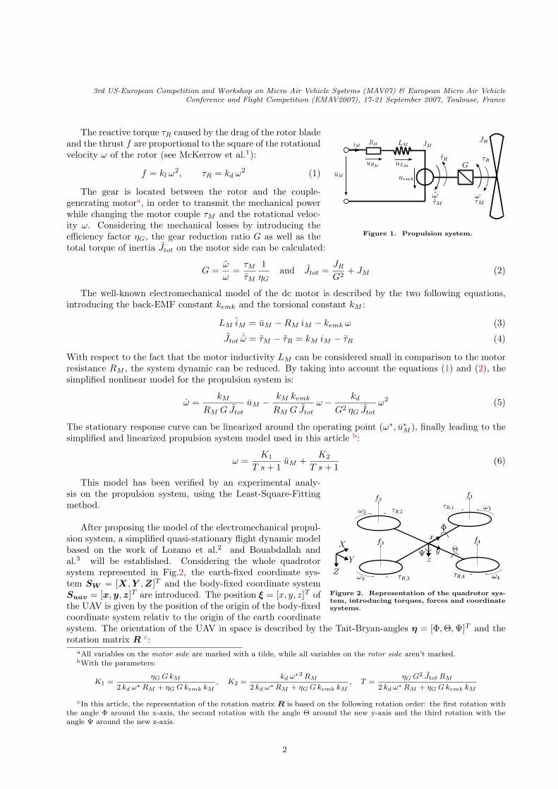
Figure 1. Propulsion system.

The reactive torque τR caused by the drag of the rotor bladeand the thrust f are proportional to the square of the rotationalvelocity ω of the rotor (see McKerrow et al.1):

f = kl ω2, τR = kd ω2 (1)

The gear is located between the rotor and the couple-generating motora, in order to transmit the mechanical powerwhile changing the motor couple τM and the rotational veloc-ity ω. Considering the mechanical losses by introducing theefficiency factor ηG, the gear reduction ratio G as well as thetotal torque of inertia Jtot on the motor side can be calculated:

G =ω

ω=

τM

τM

1

ηGand Jtot =

JR

G2+ JM (2)

The well-known electromechanical model of the dc motor is described by the two following equations,introducing the back-EMF constant kemk and the torsional constant kM :

LM iM = uM − RM iM − kemk ω (3)

Jtot˙ω = τM − τR = kM iM − τR (4)

With respect to the fact that the motor inductivity LM can be considered small in comparison to the motorresistance RM , the system dynamic can be reduced. By taking into account the equations (1) and (2), thesimplified nonlinear model for the propulsion system is:

ω =kM

RM G Jtot

uM −kM kemk

RM G Jtot

ω −kd

G2 ηG Jtot

ω2 (5)

The stationary response curve can be linearized around the operating point (ω∗, u∗M ), finally leading to the

simplified and linearized propulsion system model used in this article b:

ω =K1

T s + 1uM +

K2

T s + 1(6)

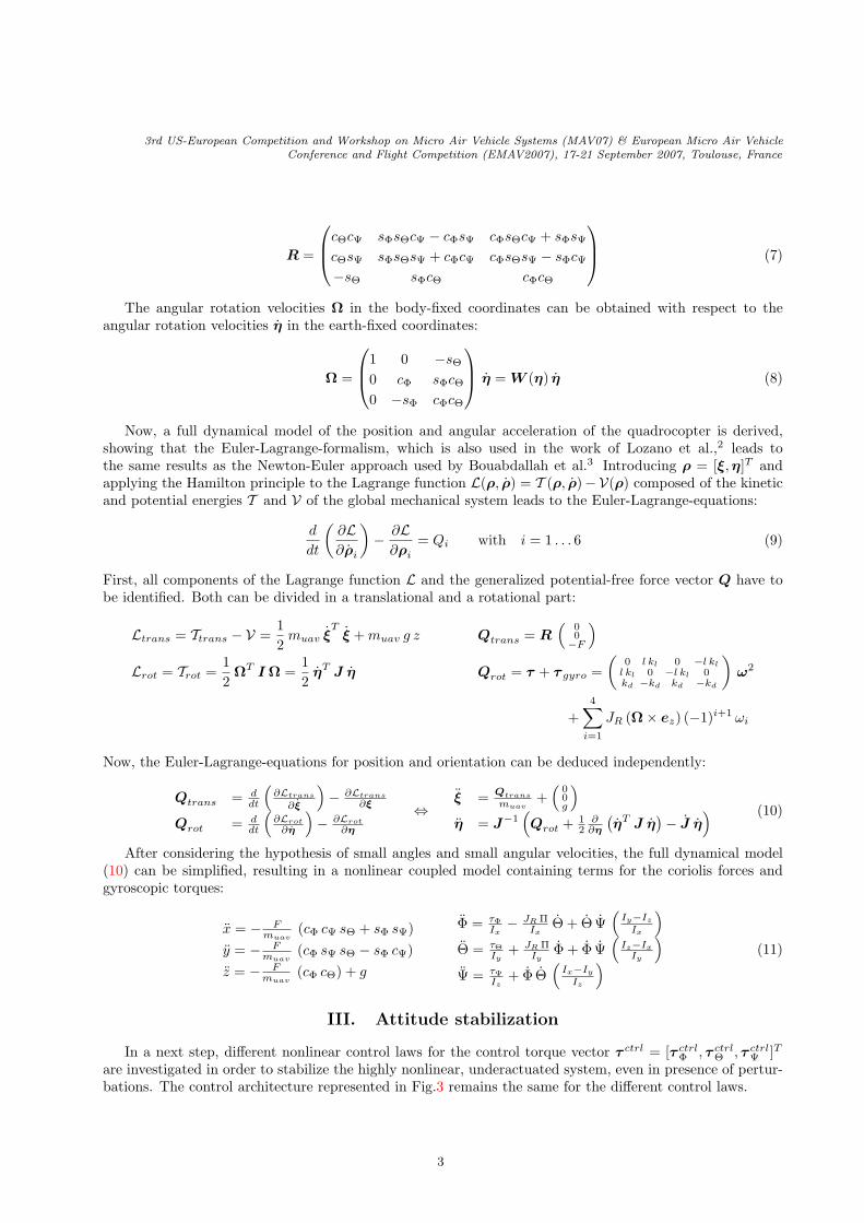
Figure 2. Representation of the quadrotor sys-tem, introducing torques, forces and coordinatesystems.

This model has been verified by an experimental analy-sis on the propulsion system, using the Least-Square-Fittingmethod.

After proposing the model of the electromechanical propul-sion system, a simplified quasi-stationary flight dynamic modelbased on the work of Lozano et al.2 and Bouabdallah andal.3 will be established. Considering the whole quadrotorsystem represented in Fig.2, the earth-fixed coordinate sys-tem SW = [X,Y ,Z]T and the body-fixed coordinate systemSuav = [x,y,z]T are introduced. The position ξ = [x, y, z]T ofthe UAV is given by the position of the origin of the body-fixedcoordinate system relativ to the origin of the earth coordinatesystem. The orientation of the UAV in space is described by the Tait-Bryan-angles η = [Φ,Θ,Ψ]T and therotation matrix R c:

aAll variables on the motor side are marked with a tilde, while all variables on the rotor side aren’t marked.bWith the parameters:

K1 =ηG G kM

2 kd ω∗ RM + ηG G kemk kM

, K2 =kd ω∗2 RM


, T =ηG G2 Jtot RM


cIn this article, the representation of the rotation matrix R is based on the following rotation order: the first rotation withthe angle Φ around the x-axis, the second rotation with the angle Θ around the new y-axis and the third rotation with theangle Ψ around the new z-axis.

2


R =

cΘcΨ sΦsΘcΨ − cΦsΨ cΦsΘcΨ + sΦsΨ

cΘsΨ sΦsΘsΨ + cΦcΨ cΦsΘsΨ − sΦcΨ

−sΘ sΦcΘ cΦcΘ

(7)

The angular rotation velocities Ω in the body-fixed coordinates can be obtained with respect to theangular rotation velocities η in the earth-fixed coordinates:

Ω =

1 0 −sΘ

0 cΦ sΦcΘ

0 −sΦ cΦcΘ

η = W (η) η (8)

Now, a full dynamical model of the position and angular acceleration of the quadrocopter is derived,showing that the Euler-Lagrange-formalism, which is also used in the work of Lozano et al.,2 leads tothe same results as the Newton-Euler approach used by Bouabdallah et al.3 Introducing ρ = [ξ,η]T andapplying the Hamilton principle to the Lagrange function L(ρ, ρ) = T (ρ, ρ)−V(ρ) composed of the kineticand potential energies T and V of the global mechanical system leads to the Euler-Lagrange-equations:

d

dt

(

∂L

∂ρi

)

−∂L

∂ρi

= Qi with i = 1 . . . 6 (9)

First, all components of the Lagrange function L and the generalized potential-free force vector Q have tobe identified. Both can be divided in a translational and a rotational part:

Ltrans = Ttrans − V =1

2muav ξ

Tξ + muav g z Qtrans = R

(

00

−F

)

Lrot = Trot =1

2Ω

T I Ω =1

2ηT J η Qrot = τ + τ gyro =

(

0 l kl 0 −l kl

l kl 0 −l kl 0kd −kd kd −kd

)

ω2

+

4∑

i=1

JR (Ω × ez) (−1)i+1 ωi

Now, the Euler-Lagrange-equations for position and orientation can be deduced independently:

Qtrans = ddt

(

∂Ltrans

∂ξ

)

− ∂Ltrans

∂ξ

Qrot = ddt

(

∂Lrot

∂η

)

− ∂Lrot

∂η

⇔ξ = Qtrans

muav+

(

00g

)

η = J−1(

Qrot + 12

∂∂η

(

ηT J η)

− J η) (10)

After considering the hypothesis of small angles and small angular velocities, the full dynamical model(10) can be simplified, resulting in a nonlinear coupled model containing terms for the coriolis forces andgyroscopic torques:

x = − Fmuav

(cΦ cΨ sΘ + sΦ sΨ)

y = − Fmuav

(cΦ sΨ sΘ − sΦ cΨ)

z = − Fmuav

(cΦ cΘ) + g

Φ = τΦ

Ix− JR Π

IxΘ + Θ Ψ

(

Iy−Iz

Ix

)

Θ = τΘ

Iy+ JR Π

IyΦ + Φ Ψ

(

Iz−Ix

Iy

)

Ψ = τΨ

Iz+ Φ Θ

(

Ix−Iy

Iz

)

(11)

III. Attitude stabilization

In a next step, different nonlinear control laws for the control torque vector τ ctrl = [τ ctrlΦ , τ ctrl

Θ , τ ctrlΨ ]T

are investigated in order to stabilize the highly nonlinear, underactuated system, even in presence of pertur-bations. The control architecture represented in Fig.3 remains the same for the different control laws.

3


Figure 3. Attitude control architecture.

First, a quaternion-based feedback controllerpresented by Tayebi et al.4 has been chosen for itsmodel parameter independent, simple implementa-tion:

τ ctrl = −µq

(

q − qd)

− µΩ (12)

with the reduced quaternion vector q = [q1, q2, q3]T ,

the positive parameter µq and the positive definite3x3 diagonal matrix µ. It is shown in4 that thecontrol law is globally asymptotically stable.

The second controller has been derived using thebackstepping approach, especially adapted to thepresent system, where the states of the rotational subsystem can be considered as inputs for the trans-lational subsystem. First, the dynamical model from (11) is rewritten as:

x1 = Φ

x2 = x1 = Φ

x2 = Φ

x3 = Θ

x4 = x3 = Θ

x4 = Θ

x5 = Ψ

x6 = x5 = Ψ

x6 = Ψ

Next, the x-coordinates are transformed into new z-coordinates by means of a diffeomorphism. This isillustrated using the x1, x2-coordinates:

z1 = x1 − xd1, z2 = x2 − xd

1 − α1(z1),

z1 = x1 − xd1 = z2 + α1(z1)

By introducing the partial lyapunov functions V1 = 12z2

1 and V2 = 12

(

z21 + z2

2

)

, it is possible to determine

the function α1(z1), two parameters a1, a2 > 0 and the control law for τΦ such that the derivate V2 ≡

−∑2

i=1 aiz2i < 0. Therefore, referring to the lyapunov stability theorem, the global asymptotical stability of

the equilibrium point z∗ = 0 is guaranteed and Φ tends to Φd. Applying this procedure to all x-coordinatesand assuming that ηd = ηd = 0 and η ≃ Ω, one obtains the following backstepping control law:

τ ctrl = − I( a1 a2−1 0 0

0 a3 a4−1 00 0 a5 a6−1

)

(η − ηd)

− I( a1+a2 0 0

0 a3+a4 00 0 a5+a6

)

Ω

(13)

In accordance with the previous work of Wendel et al.,5 it will be shown in section V that in realisticscenarios the performance of the derived backstepping controller is superior to the feedback controller.

Eventually, a new sliding mode attitude controller is proposed in this article. Based on the works of Utkin,Kondak et al. and Brandstatter et al.,6–8 this approach is more robust against parameter uncertainties andperturbations and can easily be implemented. In comparision to the work of Bouabdallah et al.,3 theproposed sliding mode controller is much simpler, shows good performances in realistic simulations of thecomplet UAV system and its stability is formally proven.Introducing the extended state vector x = [η, η]T and the input vector u = τ = [τΦ, τΘ, τΨ]T , the systembehaviour can be described as:

x = f(x) + B(x)u ⇔v = η

v = η(14)

The control error and its derivative are given by e = η−ηd, e = η− ηd = η and the switching or slidingmanifolds S are characterized by S =

x ∈ R3 | s(x) = 0

with s(x) = C1 e + C2 e, where C1,C2 are twodiagonal matrices. To achieve motion along these sliding manifolds, a discountinuous control law is used:

uctrl(x) = −K sign (s(x)) =

u+(x), s(x) > 0

u−(x), s(x) < 0(15)

4


In order to formally prove the stability of this sliding mode controller, the following two assumptionshave to be verified:

1. The system has to reach the sliding manifolds Si after a finite time, independently from the systemsinitial state x0.

2. The motion along the sliding manifolds Si must have a stable behaviour.

In order to verify the second assumption, Utkins equivalent control method will be used:6 therefore, acontinuous equivalent control variable ueq must exist and verify the condition:

min (u) ≤ ueq ≤ max (u) (16)

In the sliding mode, ueq replaces u and with (14), we have s(x) = 0 and s(x) = ∂s∂x

x = ∂s∂x

(f (x) + B ueq).Consequently, the equivalent control is given by:

ueq = −

(

∂s

∂xB

)−1∂s

∂xf (x) with

∂s

∂xB =

(

c4/Ix 0 00 c5/Iy 00 0 c6/Iz

)

(17)

The existence of ueq is guaranteed, because the inverse of ∂s∂x

B exists and the components of the term∂s∂x

f (x) could become zero only in single isolated points of the state space. Thus, the second assumptionis partially verified, only (16) has to be satisfied. To guarantee this, we consider assumption 1, which isequivalent to finding the so called domain of sliding mode and can be reduced to a stability problem withthe state vector s and the lyapunov function V (s) = sign(s)T s. Considering (14), (17) and (15), thederivative of V is:

V (s) = −K sign(s)T ∂s

∂xB sign(s) − sign(s)T ∂s

∂xB ueq

Because ∂s∂x

B is positive definite, the first term of V is confined to cmin ‖sign(s)‖2 ≤ sign(s)T ∂s∂x

B sign(s) ≤

cmax ‖sign(s)‖2 with cmin = min

c4

Ix, c5

Iy, c6

Iz

and cmax = max

c4

Ix, c5

Iy, c6

Iz

and we have:

V (s) ≤ −K cmin ‖sign(s)‖2 + ‖sign(s)T ‖ ‖∂s

∂xB‖ ‖ueq‖

Outside of the sliding manifolds Si, we have ‖sign(s)‖ ≥ 1, because at least one component si 6= 0.Therefore, the derivative of the lyapunov function is negative, when we have:

K >‖ ∂s

∂xB‖ ‖ueq‖

cmin(18)

By choosing K according to (18), the domain of sliding mode corresponds to the whole state space,verifying assumption 1. Furthermore, we will now show that (16) ⇔ −K ≤ ueq ≤ +K ⇒ ‖ueq‖ ≤ K

is satisfied by this choice of K. Considering the Frobeniusnorm ‖ ∂s∂x

B‖2F =

(

c4

Ix

)2

+(

c5

Iy

)2

+(

c6

Iz

)2

, the

stability of the sliding mode controller is formally proven, because we have:

‖ueq‖ < Kcmin

‖ ∂s∂x

B‖F

≤ K (19)

IV. Position control

Another main contribution of the present article is the design of a position controller based on thebackstepping approach. The superposition of the position controller over the attitude controller in a cascadearchitecture (shown in Fig.4) enables the robot to perform autonomous waypoint tracking: the operatoror path planner provides the desired values xd, yd, zd and Ψd and the position controller calculates thecorresponding control values Φctrl,Θctrl and F ctrl, which represent the set values of the underlying attitude

5


controller. To derive the backstepping position control law, a diffeomorphism transforms the position vectorξ = [x, y, z]T into z-coordinates. This operation will be illustrated using the x-coordinate:

z1 = x − xd, z2 = x − xd − β1(z1),

z1 = x − xd = z2 + β1(z1)

Figure 4. Cascade control architecture.

By introducing the partial lyapunov functionsV1 = 1

2z21 and V2 = 1

2

(

z21 + z2

2

)

, it is possible todetermine the function β1(z1) and two parameters

b1, b2 > 0 such that the derivate V2 ≡ −∑2

i=1 biz2i <

0:

β1 = −b1z1

V2 = z1 z1 + (z1 − β(z1))(z1 − β1) ≡ −2

∑

i=1

biz2i ⇔ z1 + z1 + b1 z1 + b2 z2 = 0

After applying the same procedure to the y

and z-coordinates and retransforming from z to ξ-coordinates, we obtain:

− Fmuav

(cΦ cΨd sΘ + sΦ sΨd) + r1 = 0

− Fmuav

(cΦ sΘ cΨd + sΦ sΨd) + r2 = 0

− Fmuav

(cΦ cΘ) + g + r3 = 0

with

r1 = (1 + b1 b2) (x − xd) + (b1 + b2) x

r2 = (1 + b3 b4) (y − yd) + (b3 + b4) y

r3 = (1 + b5 b6) (z − zd) + (b5 + b6) z

(20)Considering that xd, yd, zd and Ψd are known and η, ξ, ξ can be measured, the equations (20) can be

solved in order to determine the control variables Φctrl,Θctrl and F ctrl, d obtaining the following backsteppingposition controller:

F ctrl =muav

cΦ cΘ(r3 + g)

Φctrl = arcsin(muav

F ctrl(r1 sΨd − r2 cΨd)

)

Θctrl = arcsin

(

muav

F ctrl cΦctrl

(r1 cΨd + r2 sΨd)

)

(21)

V. Simulation and experimental results

In order to evaluate and compare the investigated control laws, various simulations have been performedon the complete closed loop system. The models for the propulsion group (6) and the flight dynamics(11) have been implemented in scilab/scicos and the following disturbances have been added: the motordynamics are delayed and bounded, the measured angles are overlaid with an additive gaussian noise (meanvalue µ = 0, standard deviation σ = 2), the digitally implemented controllers work at a frequency of 50Hz and the control output is bounded.

In the first simulation, all control laws have to stabilize the attitude of the UAV, bringing it from aninitially inclined to a horizontal configuration (ηd = 0) within approximately 1 sec: as seen in Fig.5, itappears that for this task the performance of the control laws is comparable. Furthermore, a scenario hasbeen simulated, where each controller has to track a given setpoint, bringing the attitude from the UAVfrom an initial configuration η = 0 to the desired configuration ηd = [30, 20,−45]T within approximately2 seconds: Fig.6 shows that in our simulations the necessary high gains for this short convergence time makethe behaviour of the feedback controller unstable, whereas the backstepping and sliding mode controllerbehave well.

dTo rule out trigonometric singularities, the argument of arcsin() has to be limited to [−1; 1] and the angles Φ and Θ haveto be limited to ] − π

2; +π

2[.

6


-50

-40

-30

-20

-10

0

10

20

30

40

0 0.5 1 1.5 2 2.5 3 3.5 4

Φ, Θ

, Ψ [d

eg]

Time [s]

Feedback controller, angles

ΦΘΨ

-50

-40

-30

-20

-10

0

10

20

30

40

0 0.5 1 1.5 2 2.5 3 3.5 4

Φ, Θ

, Ψ [d

eg]

Time [s]

Backstepping controller, angles

ΦΘΨ

-50

-40

-30

-20

-10

0

10

20

30

40

0 0.5 1 1.5 2 2.5 3 3.5 4

Φ, Θ

, Ψ [d

eg]

Time [s]

Sliding mode controller, angles

ΦΘΨ

-0.4

-0.3

-0.2

-0.1

0

0.1

0.2

0.3

0.4

0 0.5 1 1.5 2 2.5 3 3.5 4

τ Φct

rl , τΘ

ctrl , τ

Ψct

rl [Nm

]

Time [s]

Feedback controller, control torques

τΦctrl

τΘctrl

τΨctrl

-0.4

-0.3

-0.2

-0.1

0

0.1

0.2

0.3

0.4

0 0.5 1 1.5 2 2.5 3 3.5 4

τ Φct

rl , τΘ

ctrl , τ

Ψct

rl [Nm

]

Time [s]

Backstepping control, control torques

τΦctrl

τΘctrl

τΨctrl

-0.4

-0.3

-0.2

-0.1

0

0.1

0.2

0.3

0.4

0 0.5 1 1.5 2 2.5 3 3.5 4

τ Φct

rl , τΘ

ctrl , τ

Ψct

rl [Nm

]

Time [s]

Sliding mode controller, control torques

τΦctrl

τΘctrl

τΨctrl

Figure 5. Simulation results of the attitude stabilisation, ηd = [0, 0, 0]T . Top row: angles with feedback control (left),backstepping control (middle), sliding mode control (right). Bottom row: control torques with feedback control (left),backstepping control (middle), sliding mode control (right). Controller parameters: µx = µy = µz = 0.4, µq = 10, a1 =a2 = a4 = a6 = 7, a3 = 2, a5 = 5, K = 0.04, c1 = c3 = c5 = 1, c2 = 0.3, c4 = 0.5, c6 = 0.4

-60

-40

-20

0

20

40

0 2 4 6 8 10

Φ, Θ

, Ψ [d

eg]

Time [s]

Feedback controller, angles

ΦΘΨ

-60

-40

-20

0

20

40

0 2 4 6 8 10

Φ, Θ

, Ψ [d

eg]

Time [s]

Backstepping controller, angles

ΦΘΨ

-60

-40

-20

0

20

40

0 2 4 6 8 10

Φ, Θ

, Ψ [d

eg]

Time [s]

Sliding mode controller, angles

ΦΘΨ

-0.4

-0.3

-0.2

-0.1

0

0.1

0.2

0.3

0.4

0 2 4 6 8 10

τ Φct

rl , τΘ

ctrl , τ

Ψct

rl [Nm

]

Time [s]

Feedback controller, control torques

τΦctrl

τΘctrl

τΨctrl

-0.4

-0.3

-0.2

-0.1

0

0.1

0.2

0.3

0.4

0 0.5 1 1.5 2 2.5 3 3.5 4

τ Φct

rl , τΘ

ctrl , τ

Ψct

rl [Nm

]

Time [s]

Backstepping controller, control torques

τΦctrl

τΘctrl

τΨctrl

-0.4

-0.3

-0.2

-0.1

0

0.1

0.2

0.3

0.4

0 0.5 1 1.5 2 2.5 3 3.5 4

τ Φct

rl , τΘ

ctrl , τ

Ψct

rl [Nm

]

Time [s]

Sliding mode controller, control torques

τΦctrl

τΘctrl

τΨctrl

Figure 6. Simulation results of the setpoint tracking, ηd = [30, 20,−45]T . Top row: angles with feedback control(left), backstepping control (middle), sliding mode control (right). Bottom row: control torques with feedback control(left), backstepping control (middle), sliding mode controller (right). Controller parameters: µx = µy = µz = 0.7, µq =5, a1 = a3 = a5 = 4, a2 = a4 = a6 = 3, K = 0.03, c1 = c3 = c5 = 1, b2 = 0.4, b4 = b6 = 0.5

For the validation of the position controller, various scenarios have been simulated, showing promissingresults for an implementation on the real system. For example, the UAV has to follow a helix formedpath while rotating around his own z-axis: the simulation result is represented in Fig.7, showing the stabletracking behaviour of the complete closed loop system.

Moreover, a low cost autonomous miniature drone (represented in Fig.8) has been designed and imple-mented, using exclusively off-the-shelf components and open source software: employing a highly integratedembedded inertial measurement unit discussed in the work of Jang et al.9 and the power of a real timeonboard CPU, the backstepping control law has been implemented on the real system suspended on a tri-pod. Fig.9 shows some first test results obtained with the prototype, which is stabilized around η = 0.Improvements have still to be made on the hardware to enhance the controller dynamics, particularly withregard to the closed-loop speed control of the motors.

7


-2-1.5 -1-0.5 0 0.5 1 1.5 2 -2-1.5-1-0.5 0 0.5 1 1.5 2

-7-6-5-4-3-2-1 0

z

Desired and real trajectories (in meters)

Desired trajectoryReal trajectory

x y

z

-10

-5

0

5

10

0 10 20 30 40 50 60 70

x, y

, z [m

]

Time [s]

Position over time

xyz

-1 0 1 2 3 4 5 6 -1 0 1 2 3 4 5 6

-7-6-5-4-3-2-1 0

z

Desired and real trajectories (in meters)

Desired trajectoryReal trajectory

x y

z

-10

-5

0

5

10

0 10 20 30 40 50 60 70

x, y

, z [m

]

Time [s]

Position over time

xyz

-40

-30

-20

-10

0

10

20

30

40

0 10 20 30 40 50 60 70

Φ, Θ

[deg

]

Time [s]

Angles over time

ΦΘ

Figure 7. Simulation results of the position controller. Top row: the UAV tracks well the desired path in form of a helix(left), it’s actual position ξ is plotted (middle) and a 3D-animation (right) visualizes the simulation results. Bottom row:the UAV tracks well the desired quadratic path (left), it’s actual position ξ is plotted (middle) and the angular values Φ, Θare plotted (right). Attitude controller parameters: a1 = a2 = a3 = a4 = a5 = a6 = 7, b1 = b2 = 5, b3 = b5 = 1, b4 = b6 = 2

-30

-20

-10

0

10

20

30

0 2 4 6 8 10 12

Φ, Θ

[deg

]

Time [s]

Angles

ΦΘ

-0.1

-0.05

0

0.05

0.1

0 2 4 6 8 10 12

τ ctr

l [N

m]

Time [s]

Control torques (backstepping)

τΦτΘ

-30

-20

-10

0

10

20

30

0 2 4 6 8 10 12

Ω [d

eg/s

]

Time [s]

Angular velocity (from sensors)

ΩxΩy

Figure 9. First test results of the backstepping attitude controller.

VI. Conclusion

Figure 8. Quadrocopter prototype with anhighly integrated Inertial Measurment Unit anda ARM-based CPU running a linux OS.

In this article, a complete and a simplified model for a four-rotor flying robot have been proposed. Moreover, three differ-ent control approaches have been investigated and discussed: afeedback control law, a backstepping control law and a newlyestablished sliding mode control law. The performances havebeen analysed using various simulation results, showing therobust behaviour of the backstepping and sliding mode con-trollers regarding the stabilization and the setpoint trackingof the complete UAV model, whereas the feedback controllershows poor performance regarding the setpoint tracking. Fur-thermore, a new position controller has been proposed, permit-ting an autonomous waypoint tracking and showing promissingsimulation results. Finally, a low cost prototype has been im-plemented, showing promissing first test results.

References

1McKerrow, P., “Modelling the Draganflyer four-rotor helicopter,” IEEE International Conference on Robotics and Au-tomation, 2004 , 2004, pp. 3596– 3601.

2Escareno, J., Salazar-Cruz, S., and Lozano, R., “Embedded control of a four-rotor UAV,” Proceedings of the 2006 AmericanControl Conference Minneapolis, 2006 , 2005.

3Bouabdallah, S. and Siegwart, R., “Backstepping and Sliding-mode Techniques Applied to an Indoor Micro Quadrotor,”IEEE International Conference on Robotics and Automation, 2005 , 2005, pp. 2247– 2252.

8


4Tayebi, A. and McGilvray, S., “Attitude Stabilization of a VTOL Quadrotor Aircraft,” IEEE Transactions on controlsystems technology, 2006 , Vol. 14, 2006, pp. 562– 571.

5Wendel, J. and Bruskowski, L., “Comparison of Different Control Laws for the Stabilization of a VTOL UAV,” EuropeanMicro Air Vehicle Conference and Flight Competition 2006 25 - 26.07.2006, Braunschweig, 2006.

6Utkin, V. I., “Variable structure systems with sliding modes,” IEEE Transactions on Automatic Control , Vol. AC-22,1977, pp. 212–222.

7Kondak, K., Hommel, G., Stanczyk, B., and Buss, M., “Robust Motion Control for Robotic Systems Using Sliding Mode,”Proceedings of the IEEE/RSJ International Conference on Intelligent Robots and Systems, 2005 , 2005, pp. 2375 – 2380.

8Brandtstadter, H. and Buss, M., “Control of Electromechanical Systems using Sliding Mode Techniques,” 44th IEEEConference on Decision and Control, 2005 and 2005 European Control Conference, 2005, pp. 1947 – 1952.

9Jang, J. and Liccardo, D., “Automation of small UAVs using a low cost MEMS sensor and embedded computing platform,”25th Digital Avionics Systems Conference, 2006 , 2006.

9

Documents

Nonlinear Attitude and Position Control of a Micro Quadrotor using Sliding Mode … · 2011-02-17 · Nonlinear Attitude and Position Control of a Micro Quadrotor using Sliding Mode