Research ArticleIndoor Massive MIMO Channel Modelling UsingRay-Launching Simulation

Jialai Weng1 Xiaoming Tu1 Zhihua Lai2 Sana Salous3 and Jie Zhang1

1 Department of Electrical and Electronics Engineering University of Sheffield Sheffield S1 3JD UK2 Ranplan Wireless Network Design Ltd Sheffield S1 4DP UK3Department of Computer Science and Engineering Durham University Durham DH1 3LE UK

Correspondence should be addressed to Jialai Weng jialaiwengsheffieldacuk

Received 23 January 2014 Revised 1 June 2014 Accepted 1 July 2014 Published 6 August 2014

Academic Editor Xuefeng Yin

Copyright copy 2014 Jialai Weng et al This is an open access article distributed under the Creative Commons Attribution Licensewhich permits unrestricted use distribution and reproduction in any medium provided the original work is properly cited

Massive multi-input multioutput (MIMO) is a promising technique for the next generation of wireless communication networksIn this paper we focus on using the ray-launching based channel simulation to model massive MIMO channels We propose onedeterministic model and one statistical model for indoor massive MIMO channels both based on ray-launching simulation Wefurther propose a simplified version for eachmodel to improve computational efficiencyWe simulate themodels in indoor wirelessnetwork deployment environments and compare the simulation results with measurements Analysis and comparison show thatthese ray-launching based simulation models are efficient and accurate for massive MIMO channel modelling especially withapplication to indoor network planning and optimisation

1 Introduction

MassiveMIMO is to equip a large number of antennas at boththe transmitter and the receiver in a wireless communicationsystem It is also known as large array system MassiveMIMO has the advantage of providing both higher spectralefficiency and power efficiency Recently massive MIMO hasbeen widely accepted as a promising technique for the nextgeneration of wireless communication system [1] See [2 3]for a recent survey on the topic of massive MIMO system

Site-specific channel modelling is to model the chan-nel using the environment information and physical radiopropagation model to obtain the channel information forspecific scenarios Popular site-specific channel models areelectromagnetic propagation based methods such as finite-difference time-domain (FDTD) and ray-based methodsOne of the major applications for the site-specific channelmodels is wireless network deployment The ray-launchingalgorithm is especially suitable for this application purposedue to the modelling efficiency [4]

Wireless network planning and optimisation is the oneof the major applications of the site-specific channel models

Figure 1 shows a typical channel modelling scenario forindoor network planning To optimise the locations of thenetwork nodes such as base station a large number ofpotential locations are predicted which is computationallydemanding Furthermore large network deployment envi-ronments such as shoppingmalls and airports also pose highcomputational demands on the prediction model Thereforefor the application of network deployment and optimisationa computationally efficient channel model is highly desirable

There have been research works applying the ray-basedmodels to model MIMO channelsThe work of [5] is an earlyresearch work using ray-tracing to model MIMO channelThe work focused on the limiting factors on channel capacityin MIMO system Later the work of [6] proposed to predictMIMO channel using ray-tracing due to its computationalefficiency under the setting with a small number of antennasMoreover the work of [7] studied a similar model focusingon verification of the channel capacity results This workverified the simulation results with measurements in anindoor scenario with a 2 times 2 MIMO system Furthermorethe work of [8] also studied the MIMO channel matrix basedon ray-tracing not only channel capacity but also various

Hindawi Publishing CorporationInternational Journal of Antennas and PropagationVolume 2014 Article ID 279380 13 pageshttpdxdoiorg1011552014279380

2 International Journal of Antennas and Propagation

Figure 1 An example of channel map for indoor network planning

channel parameters such as angular and delay parametershave also been characterised based on ray-tracing modelsAs ray-tracing model can provide multipath information itcan be exploited for modelling various channel parameters inmultipath channel parameters So the work of [9] proposeda multipath channel model based on applying ray-tracingmodel The MIMO channel parameters have been furtherderived based on this model With various MIMO modelsbeing proposed thework of [10] compared the 3Dray-tracingMIMO channel models and various statistical models

The aforementioned research works of ray-based MIMOchannel modelling have all focused on modelling the con-ventional MIMO system with a small number of antennasA ray-based model specifically for massive MIMO system isstill missing Although some of the models can be applied tomodel massive MIMO channel the performance especiallythe computational efficiency is unsatisfying to the demandof network planning and optimisation purpose The primarychallenge of modelling massive MIMO channel using ray-based site-specific models especially for applications inwireless network deployment is the high computational costcaused by the large number of antennas

Another popular site-specific channel modelling tool fornetwork planning is FDTD method and related models [11]In the application of network planning and optimisationa large number of channels at different locations over theplanning space is computed for optimisation In such casesthe computational speed of the traditional 3D FDTDmodel isnot satisfying to this requirement of the applicationHoweverpurposefully designed and optimised computational efficientmodels such as the frequency domain Par-Flow model [12]lack the capability of 3D modelling which is essential to themassive MIMO channel

To address the computational efficiency challenge ofmodelling massive MIMO channel for wireless networkdeployment application we propose to apply a computation-ally efficient intelligent ray-launching algorithm (IRLA) [13]to model massive MIMO system in site-specific scenariosIts inherent 3D modelling capability and high computationalefficiency make it a highly desirable model for networkplanning and optimisation application

The purpose of the paper is to propose 2 ray-launchingbased models in massive MIMO channel modelling forindoor wireless network deployment application The firstray-launching model is a direct application of ray-launchingto massive MIMO modelling Based on the first model wefurther simplified the model by using a reference pointLater we proposed the second model based on probabilisticprinciple We also gave a simplified model based on areference point These simplified models have the advantageof computational efficiency in massive MIMO modellingFurthermore the comparison between the model simulationresults and channel measurements shows good agreements

The organisation of the paper is as follows In Section 21we establish the ray-launching based models for massiveMIMO channel In Section 3 we present the simulation andmeasurement scenarios In Section 41 we analyse and discussthe simulation results Section 5 concludes the work

2 MIMO Modelling Using Ray-Launching

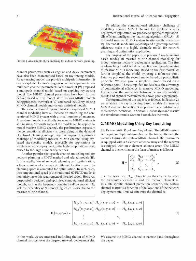
21 Deterministic Ray-Launching Model The MIMO systemis to equip multiple antennas both at the transmitter and thereceiver Figure 2 illustrates aMIMOchannelThe transmitteris equipped with a 119905-element antenna array and the receiveris equipped with an 119903-element antenna array The MIMOchannel is then written in the form of matrix as follows

H =

[[[[

[

11986711

11986712

sdot sdot sdot 1198671119903

11986721

11986722

sdot sdot sdot 1198672119903

d

1198671199051

1198671199052

sdot sdot sdot 119867119905119903

]]]]

]

(1)

The matrix element 119867119898119899

characterises the channel betweenthe transmitter element 119899 and the receiver element 119898In a site-specific channel prediction scenario the MIMOchannel matrix is a function of the locations of the networkdeployment site Thus we can write the channel as

H (119909 119910 119911 120596) =

[[[[[[[[

[

11986711(119909 119910 119911 120596) 119867

12(119909 119910 119911 120596) sdot sdot sdot 119867

1119903(119909 119910 119911 120596)

11986721(119909 119910 119911 120596) 119867

22(119909 119910 119911 120596) sdot sdot sdot 119867

2119903(119909 119910 119911 120596)

d

1198671199051(119909 119910 119911 120596) 119867

1199052(119909 119910 119911 120596) sdot sdot sdot 119867

119905119903(119909 119910 119911 120596)

]]]]]]]]

]

(2)

In this work we are interested in finding the set of MIMOchannel matrices over the targeted network deployment site

We assume the MIMO channel is narrow band throughoutthe paper

International Journal of Antennas and Propagation 3

Tx1

Tx2

Txt

Rx1

Rx2

Rxr

Figure 2 MIMO transmitter and receiver scheme

According to multipath propagation the narrow bandMIMO channel matrix elements can be written as

119867119898119899

(119909 119910 119911 120596) =

119902

sum

120572=1

119860120572(119909 119910 119911) 119890

minus1198951205960120591120572(119909119910119911) (3)

where119860120572is the amplitude of the 120572th ray 119902 is the total number

of rays 120591 is the time delay and 120591120572is the delay of the 120572th ray

and 1205960is the carrier frequency

This equation gives the channel frequency response as aresult of summation of the rays or multipath components Itis the mathematical relationship we use to obtain the channelfrom the ray-launching model

By applying this relationship the ray-launching modelcan be used to predict the set of MIMO channel matricesover the targeted network deployment site We can write thechannel frequency response as

H (119909 119910 119911 120596) = H (119909 119910 119911) (4)

where the individual channel element 119867119898119899(119909 119910 119911) is given

by (3) with a fixed value of 1205960

The channel parameters the amplitude 119860120572(119909 119910 119911) and

the delay 120591120572(119909 119910 119911) are given by the ray-launching model

based on GO and UTD The model calculates each channelelement according to (3) sequentially until all the elementsare calculated To obtain a complete set of MIMO channelmatrices of the network deployment site the prediction isrepeated over the locations of the deployment site until theset of locations (119909 119910 119911) covers the deployment site Figure 3shows an example of ray-launching model in an indoor officeenvironment

We name the above model as the deterministic modelTo further improve computational efficiency we propose asimplified model based on this model

22 Simplified Deterministic Model Using Phase-Shift Deter-ministic Phase-shiftmodel is amodel based onmodelling theMIMO channel through the array response of the receiverantenna arrayThe transmitter array and propagationmecha-nism aremodelled by the ray-launchingmodel For a receiverarray we can write the channel output in time domain as

ℎ (119905) = 119904 (119905) lowast 119903 (119905) (5)

XYZN

X

Y

Z

N

Figure 3 Ray-launching in an indoor environment

Δd5 Δd4 Δd3 Δdr2

Ant 5 Ant 4 Ant 3 Ant 2 Ant 1

Figure 4 An illustration of the phase-shift model in a linear array

where 119904(119905) is the ray arriving at the receiver array and 119903(119905) isthe array response The symbol ldquolowastrdquo represents the convolu-tion operation The total channel effect is the convolution ofthe arriving rays feed to the receiver array We can write thisrelationship in frequency domain as

H(120596) = R1015840(120596) sdot S(120596) (6)

whereH(120596) is the full channelmatrix vector S(120596) is the groupof rays arriving at the receiver array in a row vector form andR(120596) is the array response vector and the operator 1015840 is thetranspose of a row vector Vector R and vector S are both rowvectors

The array response can be written in a row vector form as

R(120596) = [1199031(120596) 119890minus2119895120587Δ1198891120582 sdot sdot sdot 119903

119903(120596) 119890minus2119895120587Δ119889119903120582] (7)

where 120582 is the wavelength of the electromagnetic wave 119903119903is

the amplitude of the array response and Δ119889119903is the distance

difference between the 119903th ray and the representative rayarriving at the reference point Together with this vectorthe formula in (6) characterises the matrix array responseby modelling the complete channel matrix as the outputof receiver array fed by arriving rays as the input Therelationship is illustrated in Figure 4

On the other hand the arriving group of rays can bewritten as

S(120596) = [1199041(120596) 1199042(120596) sdot sdot sdot 119904119905(120596)] (8)

The matrix elements in H(120596) are calculated by the ray-launching model in (3) In the direct ray-launching modelthe matrix elements are calculated sequentially until the fullchannel matrix is completed In application we notice thatsuch a way of calculating each individual channel matrix ele-ment is cumbersome and unnecessary We can approximatethe group of arriving rays by using a single representative

4 International Journal of Antennas and Propagation

12 3 4

5

1718 19 20

21

3334 35 36

37

49

50 5152

53

ha

ra

Figure 5 A cylindrical antenna array

ray If we choose the ray arriving at the array centre as therepresentative ray the above matrix can be written as

S(120596) = [119904119888(120596) 119904119888(120596) sdot sdot sdot 119904119888(120596)] (9)

where 119904119888(120596) is the ray arriving at the array center Its

exact value is determined by (3) through tracing along thepropagating rays In contrast to the model of calculating allthe individual matrix elements in (4) this model significantlyreduces the computational complexity Combining this equa-tion with (7) according to the formula in (6) we have themodel for the MIMO channel matrix asH(120596)

=

[[[[[

[

ℎ119888(120596) 119890minus211989512058711988911120582 ℎ

119888(120596) 119890minus211989512058711988912120582 sdot sdot sdot ℎ

119888(120596) 119890minus21198951205871198891119903120582

ℎ119888(120596) 119890minus211989512058711988921120582 ℎ

119888(120596) 119890minus211989512058711988922120582 sdot sdot sdot ℎ

119888(120596) 119890minus21198951205871198892119903120582

d

ℎ119888(120596) 119890minus21198951205871198891199051120582 ℎ

119888(120596) 119890minus21198951205871198891199052120582 sdot sdot sdot ℎ

119888(120596) 119890minus2119895120587119889119905119903120582

]]]]]

]

(10)

Such a simplification has been used in previous works ofMIMOmodelling based on ray-tracing [14 15] Although it isan approximation we notice that in most applications it has asatisfying degree of accuracyWewill compare themodelwiththemeasurement in Section 41 However from the computa-tional efficiency perspective this model significantly reducesthe computational complexity by reducing the repetitions ofthe ray-launching simulation to only once

Here we derive the model for the receiver array used inthemeasurement using the above phase-shiftmodel Figure 5shows a cylindrical antenna array with 4 rings of 16-elementarray mounted on the cylindrical surfaceThe radiance of thecylinder is 119903

119886and the distance between the rings is ℎ

119886

We can identify the distance differences by the geometricrelationship The distance difference has four possible values

as in (11) and (12) for the two inner rings of elements and as in(13) and (14) for the two outer rings of elements where 119889

0is

the distance between the transmitter and the array centre inthe horizontal plane120601

119894is the azimuth angle of the 119894th element

with respect to the reference direction Consider

Δ1198891= (1199032

119886+ 1198892+1

4ℎ2

119886minus ℎ119886radic1198892minus (1198890+ 119903119886)2

minus2119903 (1198890+ 119903119886) cos120601

119894)

12

(11)

Δ1198892= (1199032

119886+ 1198892+1

4ℎ2

119886+ ℎ119886radic1198892minus (1198890+ 119903119886)2

minus2119903 (1198890+ 119903119886) cos120601

119894)

12

(12)

Δ1198893= (1199032

119886+ 1198892+9

4ℎ2

119886minus 3ℎ119886radic1198892minus (1198890+ 119903119886)2

minus2119903 (1198890+ 119903119886) cos120601

119894)

12

(13)

Δ1198894= (1199032

119886+ 1198892+9

4ℎ2

119886+ 3ℎ119886radic1198892minus (1198890+ 119903119886)2

minus2119903 (1198890+ 119903119886) cos120601

119894)

12

(14)

R(120596)

= [119890minus2119895120587Δ1198893120582 sdot sdot sdot 119890

minus2119895120587Δ1198891120582 sdot sdot sdot 119890minus2119895120587Δ1198892120582 sdot sdot sdot 119890

minus2119895120587Δ1198894120582 sdot sdot sdot]

(15)

Thus the array response vector is written as (15) Inthis equation the array response can be uniformly dividedinto 4 parts corresponding to the 4 rings of elements Eachpart contains a 16-element vector corresponding to the 16elements in each ring With the ray-launching model to feedthe rays as the input we can obtain the complete channelmatrix

A similar phase-shift model has also been used in MIMOchannel modelling in [16] However using only a single rayto approximate the whole array has low accuracy especiallyfor modelling large array systems Therefore we can furtherchoose more representative rays to model the large size arrayto improve accuracy For example in the cylindrical array inFigure 5 we can model the cylindrical array as 4 layers of 2Duniform circular array Each consists of 16 antenna elementsThus instead of choosing the cylindrical array centre as thereference point we choose the centres of the 4 layers of the 2Dcircular array We then have 4 rays to approximate the wholechannel matrix

In this case the distance difference is given as

Δ119889119894(119901) = radic119903

2

119886+ 1198892(119901) minus 2119903(119889

0+ 119903119886) cos120601

119894minus 119889119894(119901)

for 119901 = 1 2 3 4 (16)

where 119901 is the 4 chosen rays and 119889119894(119901) is the distance between

the transmitter and the reference points of the 4 rays Thenthe complete array response is given as in (17) with (16) asfollows

International Journal of Antennas and Propagation 5

R(120596) = [119890minus2119895120587Δ1198891(1)120582 sdot sdot sdot 119890minus2119895120587Δ11988917(2)120582 sdot sdot sdot 119890minus2119895120587Δ11988933(3)120582 sdot sdot sdot 119890minus2119895120587Δ11988949(4)120582 sdot sdot sdot] (17)

This model requires the ray-launching simulation of 4 rays Itcompensates the accuracy by higher computational cost thanthe single ray model We name this model as the simplifieddeterministic model in the following part of this paper

23 Ray-Launching Based Statistical Model Modelling thewireless channel as a probabilistic fading channel is anothercategory of channel models in contrast to the deterministicchannel models It has the advantage of simplicity and effi-ciency when physical model is prohibitively complex In thispart we propose a probabilistic channel model for massiveMIMO based on the ray-launching model Considering thatthe model is specifically for indoor scenario we model thefading channel as Rician distribution The choice of Riciandistribution is because it comprises a rich group of probabilitydistributions by determining various values for the Rician119870factor a group of statistical distributions is includedThe ray-launching model supplies the multipath information to esti-mate the parameters for theRician distribution Furthermorethe channel measurement also indicates that the channelelements follow aRician distribution A recent study tomodelthe massive MIMO as a Rician distributed statistical modelcan be found in [17]

A single antenna Rician distributed channel can bewritten as

ℎ = radic119896ℎ119889+ radic1 minus 119896ℎ

119904 (18)

where 119896 is the119870 factor in Rician distribution ℎ119889is the direct

path component and ℎ119904is the scattering component

We model the channel matrix element 119867119898119899

in (1) as aRician distributed random variable

119867119898119899

sim Rice (V 120590) (19)

where V and 120590 are the parameters to determine the Riciandistribution The probability distribution function of theRician distribution is given as

119891 (119909 | V 120590) =119909

1205902(

minus (1199092+ 1205902)

21205902

)1198680(119909V1205902) (20)

where 1198680(sdot) is the modified Bessel function of the first kind

with order zero In order to obtain the exact distributionfunction we need to estimate the two parameters V and 120590We will resort to the ray-launching model to estimate thesetwo parameters

The ray-launchingmodel traces a group of rays equivalentto themultipath componentsThismultipath information canbe used to estimate the parameters of the Rician distributionBelow we adopt the method from the work of [18] to estimatethe Rician distribution parameters

The rays are modelled as equivalent to the multipathcomponents in (3) From this model we have the values ofthe ray field 119860

120572along each ray We can use this multipath

information to estimate the parameters V and 120590 as shownbelow

According to [18] the 119896-factor can be estimated as

119896 =radic1 minus 119903

1 minus radic1 minus 119903

(21)

The quantity 119903 is given as

119903 =

119881 [1198602]

(119864 [1198602])2 (22)

where 119881[1198602] is the variance of 1198602After obtaining the 119896-factor the Rician distribution

parameters V and 120590 can be calculated from

V2 =119896

1 + 119896Ω

1205902=

1

2 (1 + 119896)Ω

(23)

where Ω = 119864[1198602] is the expected value of the 1198602 Thus we

obtain the two parameters V and 120590Then we can write the MIMO channel matrix as

H =

[[[[[[[[[

[

11986711sim Rice (V

11 1205902

11) 11986711sim Rice (V

12 1205902

12) sdot sdot sdot 119867

1119903sim Rice (V

1119903 1205902

1119903)

11986721sim Rice (V

21 1205902

21) 11986722sim Rice (V

22 1205902

22) sdot sdot sdot 119867

2119903sim Rice (V

2119903 1205902

2119903)

d

1198671199051sim Rice (V

1199051 1205902

1199051) 1198671199052sim Rice (V

1199051 1205902

1199051) sdot sdot sdot 119867

119905119903sim Rice (V

119905119903 1205902

119905119903)

]]]]]]]]]

]

(24)

6 International Journal of Antennas and Propagation

where V119905119903

is the V parameter estimated between the 119903threceiver and the 119905th transmitter We name this model as thestatistical model in the following part of the paper

This probabilistic MIMO model requires the calculationof V and120590 parameters for each channelmatrix element Such astatistical model still requires the input from the determinis-tic ray-launchingmodel But it has the advantage of flexibilityin real application since the only parameters required arethe parameters for the probability distributions Moreoverthe calculation repeats the ray-launching simulation untilall the matrix elements are computed Such a process costshigh computational resource in simulation We can furthersimplify the calculation process in the following part

24 Simplified Statistical Model Using Phase-Shift Similar tothe simplified deterministic model for massive MIMO chan-nel we can choose one representative point to approximatethe whole antenna array Although such an approximationsacrifices certain accuracy it significantly reduces the com-putational cost by decreasing the repetition of ray-launchingmodel simulation to only once

Here again we choose the array center as the representa-tive point to calculate the probability distribution parametersV and 120590 for the whole channel matrix Thus the channelmatrix is written as

H =

[[[[[

[

11986711sim Rice (V

119888 1205902

119888) 11986711sim Rice (V

119888 1205902

119888) sdot sdot sdot 119867

1119903sim Rice (V

119888 1205902

119888)

11986721sim Rice (V

119888 1205902

119888) 11986722sim Rice (V

119888 1205902

119888) sdot sdot sdot 119867

2119903sim Rice (V

119888 1205902

119888)

d

1198671199051sim Rice (V

119888 1205902

119888) 1198671199052sim Rice (V

119888 1205902

119888) sdot sdot sdot 119867

119905119903sim Rice (V

119888 1205902

119888)

]]]]]

]

(25)

where V119888and 120590

119888are parameters estimated using the rays

between the transmitters and the center of the receiverarray Like the simplified deterministic model this modelshows adequate accuracy in many applications We namethis model the simplified statistical model We will show thecomparison result between this model and the measurementin Section 41

3 Measurement Campaigns

Small cell and heterogeneous wireless networks such asfemtocell and wireless local area network (WLAN) are themajor networks to be deployed for the next generation ofwireless networksThese small networks are mainly deployedin indoor environments as a complement to the larger cellnetworks to deploy heterogeneous networks The measure-ments are carried out in indoor environments They aretypical small cell wireless network deployment scenariosEquipped with massive MIMO antenna arrays they areinteresting scenarios for studying the performance of nextgeneration wireless networks with massive MIMO channels

We have carried out two measurement campaigns for theindoor cellular networks downlink and uplink scenariosWegive the details of the channel measurements in the followingpart of this section As our primary concern is networkplanning for indoor networks themeasurement in the uplinkscenario was carried out with the receiver at a fixed locationIn the downlink scenario the transmitter stayed in a fixedlocation

For channel modelling such 2 scenarios have little differ-ence on the channel modelling However for measurementwe intended to measure the channel with accuracy in realnetwork applications Furthermore due to the limitationof mobility of the equipment the measurements in these2 environments fall into the network application scenarios

of downlink and uplink Moreover the two environmentshave different characteristics The uplink scenario containscomplexwalls andwindows structureThedownlink scenariois relatively simple environment The two different scenariosalso showed the flexibility and adaptability of the IRLAmodel

31 Measurement of Downlink Channel The downlink chan-nel is measured in an indoor office environment The mea-surement site is in the Electrical Engineering Departmentat Lund University Sweden Figure 6 shows a map of thebuilding floor

The antenna array equipped at the transmitter is a flatpanel antenna array with 64 dual-polarised patch antennaelements Figure 8(a) shows a photo of the transmitter arrayThe receiver array is a cylindrical arraywith 64 dual-polarisedpatch antenna elements Figure 8(b) shows a photo of thereceiver arrayThese antenna arrays are both with 64 antennaelements They are typical massive MIMO antenna arraysWe choose to use these antenna arrays to carry out themeasurement campaign to study the performance of massiveMIMO channel The frequency of the channel measurementis 26GHz The transmitter power is set to be 20 dBm to40 dBm depending on the locations

The measurement has been carried out in the roomsshown in Figure 6 The transmitter is fixed at the location 119879

119909

The receivers are moved from location 1 to location 9 Thisis a typical downlink scenario in indoor small cell networksWe measure the channel matrices at the 9 locations markedin the map

32 Measurement of Uplink Channel The channel measure-ment for uplink scenario is carried out in the Departmentof Engineering and Computing Science Durham UniversityUKThemeasurement environment and the channel sounder

International Journal of Antennas and Propagation 7

2325

2324

2323

2322

2321

2320

A

2320

B

2313

2314

2315

2319

2320

C

2312

6 5 4

89

3 2 1

TX

2316

2317

2318

2326

2327

7

Figure 6 Building floor map of the downlink scenario

have also been used to measure MIMO channel with smallnumber of antennas in the work of [19] Figure 7 shows amapof the building floor

The transmitter antenna array is a 32-element antennaarray with 4 layers of 8-element uniform linear arrays Eachantenna element has an omnidirectional radiation patternThe receiver antenna array has a similar structure with 4layers of 6-element uniform linear arrays

The measurement scenario is shown as the building mapin Figure 7 The receiver is fixed at the location 119877

119909 The

transmitter is moved from location 1 to location 8 Thefrequency of of the channel measurement is 24GHzThis is atypical uplink scenario in the indoor small cell networks Wemeasure the channel matrix at the 8 locations marked in themap

4 Measurement and Simulation Comparisonand Analysis

The prediction of the channel is based on the simulationof the IRLA It has shown to achieve accuracy close toFDTD like models in indoor environment [13] Additionallyit is optimised for achieving high computational efficiencyespecially for the purpose of network planning Furtherdetails of the IRLA have been presented in the work of [13]We use the IRLA to predict the MIMO channels in thissection

For outdoor MIMO channel modelling the work of [20ndash22] focused on the MIMO modelling based on ray-tracingsimulation These works showed that diffuse scattering is akey factor in the outdoor MIMO modelling For complexoutdoor environment diffusive scattering has an impact onthe angular spread of the propagation channel and furtherdetermines the performance of theMIMOchannel Howeverfor the indoor channel the key is to model the environmentwith details The work of [23] gave an example of MIMOchannel modelling in indoor environment The authors

Table 1 Simulation settings

Number of reflections 5Number of horizontal diffractions 5Number of vertical diffractions Unlimited1

Number of transmissions Unlimited11Until signal strength is under threshold

modelled the details of the complex indoor structure usingFDTD method Combining with a ray-tracing method asatisfying result was achieved The IRLA model has shownto achieve accuracy close to FDTD like models in [13] bymodelling the details of the environment into the simulationThe model further incorporated a parameter calibrationprocess to determine the optimal values of the parameters tominimise the prediction errors

The IRLA simulation requires the detailed informationof the environmentThe environmental information includesthe structures and materials of the environments The struc-ture of the building is imported through the constructionmap of the buildings The walls doors and windows struc-tures are all included in the simulation model The construc-tion material information is provided It is matched witha material database supported by the IRLA Figure 9 givesthe 3D view of the modelled environment in the downlinkscenario The figure shows that the windows doors wallsand tables are modelled in the simulation Additionally thesimulation model settings are given in Table 1 It gives thenumber of interactions in the IRLA simulation

Although the details of the environments are included inthe model there are other factors influencing the modellingaccuracy To further improve the accuracy of the simulationa model parameter calibration process is adopted to tunethe parametersThe calibration process further optimises theaccuracy by minimising the errors between the predictionand themeasurementThe candidate values of the parameters

8 International Journal of Antennas and Propagation

1234

5

6

7

8

RX

222

224

202

2202

289

287

286

285

2201

220

201

219

Area

114sqm

LAB

Area

72sqm

Area

51sqm

Area

132sqm

Area

13sqm

Area

30sqm

Area

17sqm

Area

27sqm

Area

50sqm

Area

48sqm

Figure 7 Building floor map of the uplink scenario

(a) (b)

Figure 8 Transmitter antenna array and receiver antenna array

International Journal of Antennas and Propagation 9

Table 2 Computation time of the models

Downlink UplinkDeterministic model computation time 302 minutes 56 seconds 278 minutes 24 secondsSimplified deterministic model computation time 36 minutes 27 seconds 32 minutes 28 secondsStatistical model computation time 308 minutes 43 seconds 281 minutes 25 secondsSimplified statistical model computation time 9 minutes 29 seconds 8 minutes 30 seconds

7

Figure 9 3D view of the simulation environment of the downlinkscenario

were written in a vector form The root mean square (RMS)error between the prediction using the parameters (120583

119894 120598119895) and

the measurement was given as

RMSE119894119895=1

119903119905

119898=119903119899=119905

sum

119898=1119899=1

radic1198672

119898119899minus (119894 119895)

2

119898119899 (26)

where (119894 119895)119898119899

is the simulated channel matrix using theparameters (120583

119894 120598119895) The calibration aims to minimise this

RMS error by tuning the propagation parameters

(120583 120598) = arg min120583119894 120598119895

(RMSE119894119895)2

(27)

The calibration process is executed in an iterative waybetween the parameter estimation and the ray-launchingsimulation This calibration process was implemented usingthe simulated annealing algorithm In practice the algorithmusually converges to achieve the minimum error

41 Computational Efficiency In this section we first presentthe computation time of the 4 models using them tosimulate the downlink and uplink scenarios Table 2 showsthe computation time the 4 models take to simulate thedownlink scenario and uplink scenario We adopt the samesimulation setting as in the work of [12] The simulationresolution is set to be 01m We can see that for a massiveMIMO system the calculation of MIMO matrices for atypical indoor environment can take several hours In oursimulation Model 1 and Model 3 take about 5 hours tosimulate the whole environment The results also show thatModel 2 and Model 4 use a significant less amount oftime than Model 1 and Model 3 This is due to the lowercomputational complexity of both Model 2 and Model 4Model 1 and Model 3 both calculate each individual channelmatrix element via ray-launching while Model 2 and Model4 reduce the times of repetition for ray-launching simulation

The computational cost in the simulation is mainly due tothe ray-launching simulationThe computation time is linearin the repetition of the ray-launching simulation For Model4 the ray-launching algorithm only simulates once Model2 simulates 4 times Model 1 and Model 3 both simulate 32timesThe computation time listed in Table 2 agrees with thisanalysis

This result suggests that for time demanding tasks innetwork planning and optimisation applications both thesimplified models Model 2 and Model 4 are better choices

42 Received Signal Power The received signal power is oneof the most important parameters in network deploymentand optimisation It is closely related to the performance ofthe wireless networks According to (3) the received power ata certain location is calculated as

119875 (119909 119910 119911) =

1003817100381710038171003817100381710038171003817100381710038171003817

119902

sum

120572=1

119860120572(119909 119910 119911) 119890

minus1198951205960120591120572(119909119910119911)

1003817100381710038171003817100381710038171003817100381710038171003817

2

(28)

Figure 10 shows the comparison between the averagereceived power of the measurements and the simulationresults in the downlink scenario Figure 11 shows the samecomparison result in the uplink scenarioWe can see that bothresults show good agreements

According to (26) we use the simulated channel 119898119899

andthemeasured channel119867

119898119899to calculate the RMS errors of the

simulation models The RMS error results are presented inTables 3 and 4

The results show that the RMS errors of Model 1 andModel 3 are smaller The RMS errors of Model 2 and Model4 are higher but still mostly under 6 dB This shows that theaccuracy of Model 1 andModel 3 is higher than that of Model2 and Model 4 This is because both Model 2 and Model 4simplify the computation by using a single ray to represent thewhole array The two simplified models trade certain degreeof accuracy for computational efficiency However the resultshows that the overall accuracy of the ray-launching modelsfor massive MIMO systems is satisfying for the networkplanning and optimisation purpose

43 Distribution of Channel Elements Massive MIMO chan-nels are in a form of large channel matrix The primarymodelling target for massive MIMO is to model the largechannel matrices We have 4 models to generate the chan-nel matrices according to (4) In this section we choosethe measurement location 5 in the downlink scenario andmeasurement location 6 in the uplink scenario to show theempirical distribution of the simulated channel elements

10 International Journal of Antennas and Propagation

Table 3 Received signal power RMS error in downlink scenario

Location 1 2 3 4 5 6 7 8 9Deterministic model 32301 dB 30285 dB 34619 dB 27061 dB 31657 dB 53280 dB 23195 dB 47964 dB 33340 dBRMS errorSimplified deterministic 37594 dB 54562 dB 54561 dB 50356 dB 58612 dB 57495 dB 58634 dB 56547 dB 55598 dBmodel RMS errorStatistical model 47565 dB 49863 dB 48322 dB 49879 dB 41897 dB 57882 dB 46671 dB 49882 dB 43375 dBRMS errorSimplified statistical 59781 dB 53245 dB 54215 dB 57145 dB 58771 dB 58873 dB 53227 dB 59551 dB 57723 dBmodel RMS error

Table 4 Received signal power RMS error in uplink scenario

Location 1 2 3 4 5 6 7 8Deterministic model 29568 dB 22584 dB 36514 dB 39184 dB 23808 dB 23101 dB 28085 dB 22751 dBRMS errorSimplified deterministic 58631 dB 57761 dB 43343 dB 54475 dB 52403 dB 59712 dB 53315 dB 59882 dBmodel RMS errorStatistical model 47701 dB 42321 dB 45642 dB 54241 dB 40214 dB 40859 dB 48794 dB 49583 dBRMS errorSimplified statistical 54578 dB 53762 dB 54772 dB 56549 dB 56873 dB 50857 dB 57544 dB 57563 dBmodel RMS error

Simplified statistical model

1 2 3 4 5 6 7 8 9

minus120

minus110

minus100

minus90

minus80

minus70

minus60

minus50

minus40

minus30

Measurement locations

Rece

ived

pow

er (d

Bm)

MeasurementDeterministic modelSimplified deterministic modelStatistical model

Figure 10 Average received power in downlink

In Figure 12 we present the cumulative distributionfunction (CDF) of the simulated channel matrix elements ofthe downlink scenario in comparison with the measurement

1 2 3 4 5 6 7 8

minus90

minus80

minus70

minus60

minus50

minus40

minus30

minus20

Measurement locations

Rece

ived

pow

er (d

Bm)

MeasurementDeterministic modelSimplified deterministic modelStatistical modelSimplified statistical model

Figure 11 Average received power in uplink

Model 2 is not included in this simulation as the powerdistribution of Model 2 is determined by the choices of therays We can see that the simulated channel matrix elements

International Journal of Antennas and Propagation 11

minus65 minus64 minus63 minus62 minus61 minus60 minus59 minus58 minus57 minus560

01

02

03

04

05

06

07

08

09

1

x

Empirical (CDF)

MeasurementDeterministic modelStatistical modelSimplified Statistical model

F(X

)

Figure 12 Distribution of received power of channel elements indownlink

0

01

02

03

04

05

06

07

08

09

1Empirical (CDF)

MeasurementDeterministic modelStatistical modelSimplified Statistical model

minus64 minus63 minus62 minus61 minus60 minus59 minus58 minus57

F(X

)

X

Figure 13 Distribution of received power of channel elements inuplink

have a very close distribution to themeasured channelmatrixelements This demonstrates a good agreement between thesimulation model and the measurement

The uplink scenario result in Figure 13 shows a similarpattern as in the downlink scenario The above resultsdemonstrate that the simulation models generate channelmatrix elements with good agreements to the measurement

1 2 3 4 5 6 7 8 9

15

20

25

30

35

40

45

Measurement locations

Chan

nel c

apac

ity (b

itss

Hz)

MeasurementDeterministic modelSimplified Deterministic modelStatistical modelSimplified Statistical model

Figure 14 Channel capacity in downlink

44 Channel Capacity Results Channel capacity gain is oneof the most attractive features of the massive MIMO channelpromised to the future wireless networks In this part of theresult we present the channel capacity comparison betweenthe simulated channels and the measurement

The MIMO channel capacity is calculated according tothe equation given in [24 25] as

119862 = E(log det(I + 119875119905

1198991198730

HHlowast)) (29)

where E(sdot) represents the expectation 119875119905is the total transmit

power and 119899 is the number of transmitter antennasWe apply the above MIMO channel capacity formula to

calculate the MIMO channel capacity from both the simu-lated channel matrices and the measured channel matricesFigure 14 shows the capacity result comparison in the down-link scenario Figure 15 shows the capacity result comparisonin the uplink scenario Both figures show a good agreementin the channel capacity between the simulated results and themeasurement This demonstrates that the simulation modelsare accurate in estimating the channel capacity Thereforethe simulation models provide a reliable way to predict thechannel capacity in network planning and optimisation

5 Conclusion

In this work we first propose 2 ray-launching based simu-lation models for modelling massive MIMO channel One isdeterministic model and the other is a probabilistic modelWe further simplified the 2 models using a phase-shiftmethod The primary application of these models is networkplanning and optimisation We compare the simulationmodels with the measurement in two real small cell network

12 International Journal of Antennas and Propagation

50

45

40

35

30

251 2 3 4 5 6 7 8

Measurement locations

Chan

nel c

apac

ity (b

itss

Hz)

MeasurementDeterministic modelSimplified Deterministic modelStatistical modelSimplified Statistical model

Figure 15 Channel capacity in uplink

deployment environmentsThe comparison results show thatthe models have good agreements with the measurementThis demonstrates that these ray-launching based simulationmodels are efficient and accurate models for planning andoptimising indoor networks equipped with massive MIMOarrays

Conflict of Interests

The authors declare that they have no conflict of interestsregarding to the publication of this paper

Acknowledgments

The first author would like to thank Mr Cheng Fang DrAndres Alayon Glasunov and Professor Fredrik Tufvessonfor the measurement campaign carried out in Lund Univer-sity and Mr Nasoruddin Mohamad and Mr Adnan Cheemafor the measurement campaign carried out in DurhamUniversity The work was supported by the EU FP7 ProjectWiNDOW

References

[1] F Boccardi R W Heath Jr A Lozano T L Marzetta and PPopovski ldquoFive disruptive technology directions for 5Grdquo IEEECommunications Magazine vol 52 no 2 pp 74ndash80 2014

[2] F Rusek D Persson B K Lau et al ldquoScaling up mimoopportunities and challenges with very large arraysrdquo IEEESignal Processing Magazine vol 30 no 1 pp 40ndash60 2013

[3] E G Larsson F Tufvesson O Edfors and T L MarzettaldquoMassive MIMO for next generation wireless systemsrdquo IEEECommunications Magazine vol 52 no 2 pp 186ndash195 2014

[4] Z Lai N Bessis G de la Roche P Kuonen J Zhang andG Clapworthy ldquoOn the use of an intelligent ray launching forindoor scenariosrdquo in Proceedings of the 4th European Conferenceon Antennas and Propagation (EuCAP rsquo10) pp 1ndash5 April 2010

[5] A Burr ldquoEvaluation of capacity of indoor wireless mimo chan-nel using ray tracingrdquo in Proceedings of the International ZurichSeminar on Broadband Communications Access TransmissionNetworking pp 28-1ndash28-6 2002

[6] S- Oh and N- Myung ldquoMIMO channel estimation methodusing ray-tracing propagation modelrdquo Electronics Letters vol40 no 21 pp 1350ndash1352 2004

[7] Y Gao X Chen and C Parini ldquoExperimental evaluationof indoor mimo channel capacity based on ray tracingrdquo inProceedings of the London Communications Symposium pp189ndash192 University College London 2004

[8] O Stabler ldquoMimo channel characteristics computed with 3dray tracing modelrdquo in Proceedings of the COST2100 TD(08)Workshop Trondheim Norway June 2008

[9] S Loredo A Rodrıguez-Alonso and R P Torres ldquoIndoorMIMO channel modeling by rigorous GOUTD-based raytracingrdquo IEEE Transactions on Vehicular Technology vol 57 no2 pp 680ndash692 2008

[10] R Hoppe J Ramuh H Buddendick O Stabler and G WolfleldquoComparison of MIMO channel characteristics computed by3D ray tracing and statistical modelsrdquo in Proceedings of the2nd EuropeanConference onAntennas and Propagation (EuCAPrsquo07) pp 1ndash5 November 2007

[11] J Gorce K Jaffres-Runser and G de la Roche ldquoDeterministicapproach for fast simulations of indoor radio wave propaga-tionrdquo IEEE Transactions on Antennas and Propagation vol 55no 3 pp 938ndash948 2007

[12] X Tu H Hu Z Lai J-M Gorce and J Zhang ldquoPerformancecomparison of MR-FDPF and ray launching in an indoor officescenariordquo in Proceedings of the Loughborough Antennas andPropagation Conference (LAPC 13) pp 424ndash428 Loughbor-ough UK November 2013

[13] Z Lai G De La Roche N BESSIS et al ldquoIntelligent raylaunching algorithm for indoor scenariosrdquo Radioengineeringvol 20 no 2 pp 398ndash408 2011

[14] B Clerckx and C OestgesMIMOWireless Networks ChannelsTechniques and Standards for Multi-Antenna Multi-User andMulti-Cell Systems Academic Press 2nd edition 2013

[15] G German Q Spencer L Swindlehurst and R ValenzuelaldquoWireless indoor channel modeling Statistical agreement ofray tracing simulations and channel sounding measurementsrdquoin Proceedings of IEEE Interntional Conference on AcousticsSpeech and Signal Processing (ICASSP rsquo01) vol 4 pp 2501ndash2504May 2001

[16] J Voigt R Fritzsche and J Schueler ldquoOptimal antenna typeselection in a real SU-MIMO network planning scenariordquo inProceedings of the 70th IEEE Vehicular Technology Conference(VTC rsquo09) pp 1ndash5 September 2009

[17] S Payami and F Tufvesson ldquoChannel measurements andanalysis for very large array systems at 26 GHzrdquo in Proceedingsof the 6th European Conference on Antennas and Propagation(EuCAP rsquo12) pp 433ndash437 March 2012

[18] A Abdi C Tepedelenlioglu M Kaveh and G GiannakisldquoOn the estimation of the K parameter for the rice fadingdistributionrdquo IEEECommunications Letters vol 5 no 3 pp 92ndash94 2001

[19] N Razavi-Ghods and S Salous ldquoWideband mimo channelcharacterization in tv studios and inside buildings in the 2225

International Journal of Antennas and Propagation 13

ghz frequency bandrdquo Radio Science vol 44 no 5 Article ID1010292008RS004095 pp 10ndash1029 2009

[20] A Richter J Salmi and V Koivunen ldquoDistributed scattering inradio channels and its contribution toMIMO channel capacityrdquoin Proceedings of the European Conference on Antennas andPropagation (EuCAP rsquo06) pp 1ndash7 Nice France November2006

[21] FMani F Quitin and C Oestges ldquoDirectional spreads of densemultipath components in indoor environments experimentalvalidation of a Ray-Tracing approachrdquo IEEE Transactions onAntennas and Propagation vol 60 no 7 pp 3389ndash3396 2012

[22] E Vitucci V Degli-Esposti and F Fuschini ldquoMimo channelcharacterization through ray tracing simulationrdquo in Proceedingsof the 1st European Conference on Antennas and Propagation(EuCAP rsquo06) pp 1ndash6 November 2006

[23] Z Yun M Iskander and Z Zhang ldquoMimo capacity calculationand fading estimation for indooroutdoor wireless commu-nication environmentsrdquo in Proceedings of the IEEE TopicalConference on Wireless Communication Technology pp 259ndash260 October 2003

[24] E Telatar ldquoCapacity of multi-antenna Gaussian channelsrdquoEuropean Transactions on Telecommunications vol 10 no 6 pp585ndash595 1999

[25] G J Foschini and M J Gans ldquoOn limits of wireless communi-cations in a fading environment when usingmultiple antennasrdquoWireless Personal Communications vol 6 no 3 pp 311ndash3351998

International Journal of

AerospaceEngineeringHindawi Publishing Corporationhttpwwwhindawicom Volume 2014

RoboticsJournal of

Hindawi Publishing Corporationhttpwwwhindawicom Volume 2014

Hindawi Publishing Corporationhttpwwwhindawicom Volume 2014

Active and Passive Electronic Components

Control Scienceand Engineering

Journal of

Hindawi Publishing Corporationhttpwwwhindawicom Volume 2014

International Journal of

RotatingMachinery

Hindawi Publishing Corporationhttpwwwhindawicom Volume 2014

Hindawi Publishing Corporation httpwwwhindawicom

Journal ofEngineeringVolume 2014

Submit your manuscripts athttpwwwhindawicom

VLSI Design

Hindawi Publishing Corporationhttpwwwhindawicom Volume 2014

Hindawi Publishing Corporationhttpwwwhindawicom Volume 2014

Shock and Vibration

Hindawi Publishing Corporationhttpwwwhindawicom Volume 2014

Civil EngineeringAdvances in

Acoustics and VibrationAdvances in

Hindawi Publishing Corporationhttpwwwhindawicom Volume 2014

Hindawi Publishing Corporationhttpwwwhindawicom Volume 2014

Electrical and Computer Engineering

Journal of

Advances inOptoElectronics

Hindawi Publishing Corporation httpwwwhindawicom

Volume 2014

The Scientific World JournalHindawi Publishing Corporation httpwwwhindawicom Volume 2014

SensorsJournal of

Hindawi Publishing Corporationhttpwwwhindawicom Volume 2014

Modelling amp Simulation in EngineeringHindawi Publishing Corporation httpwwwhindawicom Volume 2014

Hindawi Publishing Corporationhttpwwwhindawicom Volume 2014

Chemical EngineeringInternational Journal of Antennas and

Propagation

International Journal of

Hindawi Publishing Corporationhttpwwwhindawicom Volume 2014

Hindawi Publishing Corporationhttpwwwhindawicom Volume 2014

Navigation and Observation

International Journal of

Hindawi Publishing Corporationhttpwwwhindawicom Volume 2014

DistributedSensor Networks

International Journal of

2 International Journal of Antennas and Propagation

Figure 1 An example of channel map for indoor network planning

channel parameters such as angular and delay parametershave also been characterised based on ray-tracing modelsAs ray-tracing model can provide multipath information itcan be exploited for modelling various channel parameters inmultipath channel parameters So the work of [9] proposeda multipath channel model based on applying ray-tracingmodel The MIMO channel parameters have been furtherderived based on this model With various MIMO modelsbeing proposed thework of [10] compared the 3Dray-tracingMIMO channel models and various statistical models

The aforementioned research works of ray-based MIMOchannel modelling have all focused on modelling the con-ventional MIMO system with a small number of antennasA ray-based model specifically for massive MIMO system isstill missing Although some of the models can be applied tomodel massive MIMO channel the performance especiallythe computational efficiency is unsatisfying to the demandof network planning and optimisation purpose The primarychallenge of modelling massive MIMO channel using ray-based site-specific models especially for applications inwireless network deployment is the high computational costcaused by the large number of antennas

Another popular site-specific channel modelling tool fornetwork planning is FDTD method and related models [11]In the application of network planning and optimisationa large number of channels at different locations over theplanning space is computed for optimisation In such casesthe computational speed of the traditional 3D FDTDmodel isnot satisfying to this requirement of the applicationHoweverpurposefully designed and optimised computational efficientmodels such as the frequency domain Par-Flow model [12]lack the capability of 3D modelling which is essential to themassive MIMO channel

To address the computational efficiency challenge ofmodelling massive MIMO channel for wireless networkdeployment application we propose to apply a computation-ally efficient intelligent ray-launching algorithm (IRLA) [13]to model massive MIMO system in site-specific scenariosIts inherent 3D modelling capability and high computationalefficiency make it a highly desirable model for networkplanning and optimisation application

The purpose of the paper is to propose 2 ray-launchingbased models in massive MIMO channel modelling forindoor wireless network deployment application The firstray-launching model is a direct application of ray-launchingto massive MIMO modelling Based on the first model wefurther simplified the model by using a reference pointLater we proposed the second model based on probabilisticprinciple We also gave a simplified model based on areference point These simplified models have the advantageof computational efficiency in massive MIMO modellingFurthermore the comparison between the model simulationresults and channel measurements shows good agreements

The organisation of the paper is as follows In Section 21we establish the ray-launching based models for massiveMIMO channel In Section 3 we present the simulation andmeasurement scenarios In Section 41 we analyse and discussthe simulation results Section 5 concludes the work

2 MIMO Modelling Using Ray-Launching

21 Deterministic Ray-Launching Model The MIMO systemis to equip multiple antennas both at the transmitter and thereceiver Figure 2 illustrates aMIMOchannelThe transmitteris equipped with a 119905-element antenna array and the receiveris equipped with an 119903-element antenna array The MIMOchannel is then written in the form of matrix as follows

H =

[[[[

[

11986711

11986712

sdot sdot sdot 1198671119903

11986721

11986722

sdot sdot sdot 1198672119903

d

1198671199051

1198671199052

sdot sdot sdot 119867119905119903

]]]]

]

(1)

The matrix element 119867119898119899

characterises the channel betweenthe transmitter element 119899 and the receiver element 119898In a site-specific channel prediction scenario the MIMOchannel matrix is a function of the locations of the networkdeployment site Thus we can write the channel as

H (119909 119910 119911 120596) =

[[[[[[[[

[

11986711(119909 119910 119911 120596) 119867

12(119909 119910 119911 120596) sdot sdot sdot 119867

1119903(119909 119910 119911 120596)

11986721(119909 119910 119911 120596) 119867

22(119909 119910 119911 120596) sdot sdot sdot 119867

2119903(119909 119910 119911 120596)

d

1198671199051(119909 119910 119911 120596) 119867

1199052(119909 119910 119911 120596) sdot sdot sdot 119867

119905119903(119909 119910 119911 120596)

]]]]]]]]

]

(2)

In this work we are interested in finding the set of MIMOchannel matrices over the targeted network deployment site

We assume the MIMO channel is narrow band throughoutthe paper

International Journal of Antennas and Propagation 3

Tx1

Tx2

Txt

Rx1

Rx2

Rxr

Figure 2 MIMO transmitter and receiver scheme

According to multipath propagation the narrow bandMIMO channel matrix elements can be written as

119867119898119899

(119909 119910 119911 120596) =

119902

sum

120572=1

119860120572(119909 119910 119911) 119890

minus1198951205960120591120572(119909119910119911) (3)

where119860120572is the amplitude of the 120572th ray 119902 is the total number

of rays 120591 is the time delay and 120591120572is the delay of the 120572th ray

and 1205960is the carrier frequency

This equation gives the channel frequency response as aresult of summation of the rays or multipath components Itis the mathematical relationship we use to obtain the channelfrom the ray-launching model

By applying this relationship the ray-launching modelcan be used to predict the set of MIMO channel matricesover the targeted network deployment site We can write thechannel frequency response as

H (119909 119910 119911 120596) = H (119909 119910 119911) (4)

where the individual channel element 119867119898119899(119909 119910 119911) is given

by (3) with a fixed value of 1205960

The channel parameters the amplitude 119860120572(119909 119910 119911) and

the delay 120591120572(119909 119910 119911) are given by the ray-launching model

based on GO and UTD The model calculates each channelelement according to (3) sequentially until all the elementsare calculated To obtain a complete set of MIMO channelmatrices of the network deployment site the prediction isrepeated over the locations of the deployment site until theset of locations (119909 119910 119911) covers the deployment site Figure 3shows an example of ray-launching model in an indoor officeenvironment

We name the above model as the deterministic modelTo further improve computational efficiency we propose asimplified model based on this model

22 Simplified Deterministic Model Using Phase-Shift Deter-ministic Phase-shiftmodel is amodel based onmodelling theMIMO channel through the array response of the receiverantenna arrayThe transmitter array and propagationmecha-nism aremodelled by the ray-launchingmodel For a receiverarray we can write the channel output in time domain as

ℎ (119905) = 119904 (119905) lowast 119903 (119905) (5)

XYZN

X

Y

Z

N

Figure 3 Ray-launching in an indoor environment

Δd5 Δd4 Δd3 Δdr2

Ant 5 Ant 4 Ant 3 Ant 2 Ant 1

Figure 4 An illustration of the phase-shift model in a linear array

where 119904(119905) is the ray arriving at the receiver array and 119903(119905) isthe array response The symbol ldquolowastrdquo represents the convolu-tion operation The total channel effect is the convolution ofthe arriving rays feed to the receiver array We can write thisrelationship in frequency domain as

H(120596) = R1015840(120596) sdot S(120596) (6)

whereH(120596) is the full channelmatrix vector S(120596) is the groupof rays arriving at the receiver array in a row vector form andR(120596) is the array response vector and the operator 1015840 is thetranspose of a row vector Vector R and vector S are both rowvectors

The array response can be written in a row vector form as

R(120596) = [1199031(120596) 119890minus2119895120587Δ1198891120582 sdot sdot sdot 119903

119903(120596) 119890minus2119895120587Δ119889119903120582] (7)

where 120582 is the wavelength of the electromagnetic wave 119903119903is

the amplitude of the array response and Δ119889119903is the distance

difference between the 119903th ray and the representative rayarriving at the reference point Together with this vectorthe formula in (6) characterises the matrix array responseby modelling the complete channel matrix as the outputof receiver array fed by arriving rays as the input Therelationship is illustrated in Figure 4

On the other hand the arriving group of rays can bewritten as

S(120596) = [1199041(120596) 1199042(120596) sdot sdot sdot 119904119905(120596)] (8)

The matrix elements in H(120596) are calculated by the ray-launching model in (3) In the direct ray-launching modelthe matrix elements are calculated sequentially until the fullchannel matrix is completed In application we notice thatsuch a way of calculating each individual channel matrix ele-ment is cumbersome and unnecessary We can approximatethe group of arriving rays by using a single representative

4 International Journal of Antennas and Propagation

12 3 4

5

1718 19 20

21

3334 35 36

37

49

50 5152

53

ha

ra

Figure 5 A cylindrical antenna array

ray If we choose the ray arriving at the array centre as therepresentative ray the above matrix can be written as

S(120596) = [119904119888(120596) 119904119888(120596) sdot sdot sdot 119904119888(120596)] (9)

where 119904119888(120596) is the ray arriving at the array center Its

exact value is determined by (3) through tracing along thepropagating rays In contrast to the model of calculating allthe individual matrix elements in (4) this model significantlyreduces the computational complexity Combining this equa-tion with (7) according to the formula in (6) we have themodel for the MIMO channel matrix asH(120596)

=

[[[[[

[

ℎ119888(120596) 119890minus211989512058711988911120582 ℎ

119888(120596) 119890minus211989512058711988912120582 sdot sdot sdot ℎ

119888(120596) 119890minus21198951205871198891119903120582

ℎ119888(120596) 119890minus211989512058711988921120582 ℎ

119888(120596) 119890minus211989512058711988922120582 sdot sdot sdot ℎ

119888(120596) 119890minus21198951205871198892119903120582

d

ℎ119888(120596) 119890minus21198951205871198891199051120582 ℎ

119888(120596) 119890minus21198951205871198891199052120582 sdot sdot sdot ℎ

119888(120596) 119890minus2119895120587119889119905119903120582

]]]]]

]

(10)

Such a simplification has been used in previous works ofMIMOmodelling based on ray-tracing [14 15] Although it isan approximation we notice that in most applications it has asatisfying degree of accuracyWewill compare themodelwiththemeasurement in Section 41 However from the computa-tional efficiency perspective this model significantly reducesthe computational complexity by reducing the repetitions ofthe ray-launching simulation to only once

Here we derive the model for the receiver array used inthemeasurement using the above phase-shiftmodel Figure 5shows a cylindrical antenna array with 4 rings of 16-elementarray mounted on the cylindrical surfaceThe radiance of thecylinder is 119903

119886and the distance between the rings is ℎ

119886

We can identify the distance differences by the geometricrelationship The distance difference has four possible values

as in (11) and (12) for the two inner rings of elements and as in(13) and (14) for the two outer rings of elements where 119889

0is

the distance between the transmitter and the array centre inthe horizontal plane120601

119894is the azimuth angle of the 119894th element

with respect to the reference direction Consider

Δ1198891= (1199032

119886+ 1198892+1

4ℎ2

119886minus ℎ119886radic1198892minus (1198890+ 119903119886)2

minus2119903 (1198890+ 119903119886) cos120601

119894)

12

(11)

Δ1198892= (1199032

119886+ 1198892+1

4ℎ2

119886+ ℎ119886radic1198892minus (1198890+ 119903119886)2

minus2119903 (1198890+ 119903119886) cos120601

119894)

12

(12)

Δ1198893= (1199032

119886+ 1198892+9

4ℎ2

119886minus 3ℎ119886radic1198892minus (1198890+ 119903119886)2

minus2119903 (1198890+ 119903119886) cos120601

119894)

12

(13)

Δ1198894= (1199032

119886+ 1198892+9

4ℎ2

119886+ 3ℎ119886radic1198892minus (1198890+ 119903119886)2

minus2119903 (1198890+ 119903119886) cos120601

119894)

12

(14)

R(120596)

= [119890minus2119895120587Δ1198893120582 sdot sdot sdot 119890

minus2119895120587Δ1198891120582 sdot sdot sdot 119890minus2119895120587Δ1198892120582 sdot sdot sdot 119890

minus2119895120587Δ1198894120582 sdot sdot sdot]

(15)

Thus the array response vector is written as (15) Inthis equation the array response can be uniformly dividedinto 4 parts corresponding to the 4 rings of elements Eachpart contains a 16-element vector corresponding to the 16elements in each ring With the ray-launching model to feedthe rays as the input we can obtain the complete channelmatrix

A similar phase-shift model has also been used in MIMOchannel modelling in [16] However using only a single rayto approximate the whole array has low accuracy especiallyfor modelling large array systems Therefore we can furtherchoose more representative rays to model the large size arrayto improve accuracy For example in the cylindrical array inFigure 5 we can model the cylindrical array as 4 layers of 2Duniform circular array Each consists of 16 antenna elementsThus instead of choosing the cylindrical array centre as thereference point we choose the centres of the 4 layers of the 2Dcircular array We then have 4 rays to approximate the wholechannel matrix

In this case the distance difference is given as

Δ119889119894(119901) = radic119903

2

119886+ 1198892(119901) minus 2119903(119889

0+ 119903119886) cos120601

119894minus 119889119894(119901)

for 119901 = 1 2 3 4 (16)

where 119901 is the 4 chosen rays and 119889119894(119901) is the distance between

the transmitter and the reference points of the 4 rays Thenthe complete array response is given as in (17) with (16) asfollows

International Journal of Antennas and Propagation 5

R(120596) = [119890minus2119895120587Δ1198891(1)120582 sdot sdot sdot 119890minus2119895120587Δ11988917(2)120582 sdot sdot sdot 119890minus2119895120587Δ11988933(3)120582 sdot sdot sdot 119890minus2119895120587Δ11988949(4)120582 sdot sdot sdot] (17)

This model requires the ray-launching simulation of 4 rays Itcompensates the accuracy by higher computational cost thanthe single ray model We name this model as the simplifieddeterministic model in the following part of this paper

23 Ray-Launching Based Statistical Model Modelling thewireless channel as a probabilistic fading channel is anothercategory of channel models in contrast to the deterministicchannel models It has the advantage of simplicity and effi-ciency when physical model is prohibitively complex In thispart we propose a probabilistic channel model for massiveMIMO based on the ray-launching model Considering thatthe model is specifically for indoor scenario we model thefading channel as Rician distribution The choice of Riciandistribution is because it comprises a rich group of probabilitydistributions by determining various values for the Rician119870factor a group of statistical distributions is includedThe ray-launching model supplies the multipath information to esti-mate the parameters for theRician distribution Furthermorethe channel measurement also indicates that the channelelements follow aRician distribution A recent study tomodelthe massive MIMO as a Rician distributed statistical modelcan be found in [17]

A single antenna Rician distributed channel can bewritten as

ℎ = radic119896ℎ119889+ radic1 minus 119896ℎ

119904 (18)

where 119896 is the119870 factor in Rician distribution ℎ119889is the direct

path component and ℎ119904is the scattering component

We model the channel matrix element 119867119898119899

in (1) as aRician distributed random variable

119867119898119899

sim Rice (V 120590) (19)

where V and 120590 are the parameters to determine the Riciandistribution The probability distribution function of theRician distribution is given as

119891 (119909 | V 120590) =119909

1205902(

minus (1199092+ 1205902)

21205902

)1198680(119909V1205902) (20)

where 1198680(sdot) is the modified Bessel function of the first kind

with order zero In order to obtain the exact distributionfunction we need to estimate the two parameters V and 120590We will resort to the ray-launching model to estimate thesetwo parameters

The ray-launchingmodel traces a group of rays equivalentto themultipath componentsThismultipath information canbe used to estimate the parameters of the Rician distributionBelow we adopt the method from the work of [18] to estimatethe Rician distribution parameters

The rays are modelled as equivalent to the multipathcomponents in (3) From this model we have the values ofthe ray field 119860

120572along each ray We can use this multipath

information to estimate the parameters V and 120590 as shownbelow

According to [18] the 119896-factor can be estimated as

119896 =radic1 minus 119903

1 minus radic1 minus 119903

(21)

The quantity 119903 is given as

119903 =

119881 [1198602]

(119864 [1198602])2 (22)

where 119881[1198602] is the variance of 1198602After obtaining the 119896-factor the Rician distribution

parameters V and 120590 can be calculated from

V2 =119896

1 + 119896Ω

1205902=

1

2 (1 + 119896)Ω

(23)

where Ω = 119864[1198602] is the expected value of the 1198602 Thus we

obtain the two parameters V and 120590Then we can write the MIMO channel matrix as

H =

[[[[[[[[[

[

11986711sim Rice (V

11 1205902

11) 11986711sim Rice (V

12 1205902

12) sdot sdot sdot 119867

1119903sim Rice (V

1119903 1205902

1119903)

11986721sim Rice (V

21 1205902

21) 11986722sim Rice (V

22 1205902

22) sdot sdot sdot 119867

2119903sim Rice (V

2119903 1205902

2119903)

d

1198671199051sim Rice (V

1199051 1205902

1199051) 1198671199052sim Rice (V

1199051 1205902

1199051) sdot sdot sdot 119867

119905119903sim Rice (V

119905119903 1205902

119905119903)

]]]]]]]]]

]

(24)

6 International Journal of Antennas and Propagation

where V119905119903

is the V parameter estimated between the 119903threceiver and the 119905th transmitter We name this model as thestatistical model in the following part of the paper

This probabilistic MIMO model requires the calculationof V and120590 parameters for each channelmatrix element Such astatistical model still requires the input from the determinis-tic ray-launchingmodel But it has the advantage of flexibilityin real application since the only parameters required arethe parameters for the probability distributions Moreoverthe calculation repeats the ray-launching simulation untilall the matrix elements are computed Such a process costshigh computational resource in simulation We can furthersimplify the calculation process in the following part

24 Simplified Statistical Model Using Phase-Shift Similar tothe simplified deterministic model for massive MIMO chan-nel we can choose one representative point to approximatethe whole antenna array Although such an approximationsacrifices certain accuracy it significantly reduces the com-putational cost by decreasing the repetition of ray-launchingmodel simulation to only once

Here again we choose the array center as the representa-tive point to calculate the probability distribution parametersV and 120590 for the whole channel matrix Thus the channelmatrix is written as

H =

[[[[[

[

11986711sim Rice (V

119888 1205902

119888) 11986711sim Rice (V

119888 1205902

119888) sdot sdot sdot 119867

1119903sim Rice (V

119888 1205902

119888)

11986721sim Rice (V

119888 1205902

119888) 11986722sim Rice (V

119888 1205902

119888) sdot sdot sdot 119867

2119903sim Rice (V

119888 1205902

119888)

d

1198671199051sim Rice (V

119888 1205902

119888) 1198671199052sim Rice (V

119888 1205902

119888) sdot sdot sdot 119867

119905119903sim Rice (V

119888 1205902

119888)

]]]]]

]

(25)

where V119888and 120590

119888are parameters estimated using the rays

between the transmitters and the center of the receiverarray Like the simplified deterministic model this modelshows adequate accuracy in many applications We namethis model the simplified statistical model We will show thecomparison result between this model and the measurementin Section 41

3 Measurement Campaigns

Small cell and heterogeneous wireless networks such asfemtocell and wireless local area network (WLAN) are themajor networks to be deployed for the next generation ofwireless networksThese small networks are mainly deployedin indoor environments as a complement to the larger cellnetworks to deploy heterogeneous networks The measure-ments are carried out in indoor environments They aretypical small cell wireless network deployment scenariosEquipped with massive MIMO antenna arrays they areinteresting scenarios for studying the performance of nextgeneration wireless networks with massive MIMO channels

We have carried out two measurement campaigns for theindoor cellular networks downlink and uplink scenariosWegive the details of the channel measurements in the followingpart of this section As our primary concern is networkplanning for indoor networks themeasurement in the uplinkscenario was carried out with the receiver at a fixed locationIn the downlink scenario the transmitter stayed in a fixedlocation

For channel modelling such 2 scenarios have little differ-ence on the channel modelling However for measurementwe intended to measure the channel with accuracy in realnetwork applications Furthermore due to the limitationof mobility of the equipment the measurements in these2 environments fall into the network application scenarios

of downlink and uplink Moreover the two environmentshave different characteristics The uplink scenario containscomplexwalls andwindows structureThedownlink scenariois relatively simple environment The two different scenariosalso showed the flexibility and adaptability of the IRLAmodel

31 Measurement of Downlink Channel The downlink chan-nel is measured in an indoor office environment The mea-surement site is in the Electrical Engineering Departmentat Lund University Sweden Figure 6 shows a map of thebuilding floor

The antenna array equipped at the transmitter is a flatpanel antenna array with 64 dual-polarised patch antennaelements Figure 8(a) shows a photo of the transmitter arrayThe receiver array is a cylindrical arraywith 64 dual-polarisedpatch antenna elements Figure 8(b) shows a photo of thereceiver arrayThese antenna arrays are both with 64 antennaelements They are typical massive MIMO antenna arraysWe choose to use these antenna arrays to carry out themeasurement campaign to study the performance of massiveMIMO channel The frequency of the channel measurementis 26GHz The transmitter power is set to be 20 dBm to40 dBm depending on the locations

The measurement has been carried out in the roomsshown in Figure 6 The transmitter is fixed at the location 119879

119909

The receivers are moved from location 1 to location 9 Thisis a typical downlink scenario in indoor small cell networksWe measure the channel matrices at the 9 locations markedin the map

32 Measurement of Uplink Channel The channel measure-ment for uplink scenario is carried out in the Departmentof Engineering and Computing Science Durham UniversityUKThemeasurement environment and the channel sounder

International Journal of Antennas and Propagation 7

2325

2324

2323

2322

2321

2320

A

2320

B

2313

2314

2315

2319

2320

C

2312

6 5 4

89

3 2 1

TX

2316

2317

2318

2326

2327

7

Figure 6 Building floor map of the downlink scenario

have also been used to measure MIMO channel with smallnumber of antennas in the work of [19] Figure 7 shows amapof the building floor

The transmitter antenna array is a 32-element antennaarray with 4 layers of 8-element uniform linear arrays Eachantenna element has an omnidirectional radiation patternThe receiver antenna array has a similar structure with 4layers of 6-element uniform linear arrays

The measurement scenario is shown as the building mapin Figure 7 The receiver is fixed at the location 119877

119909 The

transmitter is moved from location 1 to location 8 Thefrequency of of the channel measurement is 24GHzThis is atypical uplink scenario in the indoor small cell networks Wemeasure the channel matrix at the 8 locations marked in themap

4 Measurement and Simulation Comparisonand Analysis

The prediction of the channel is based on the simulationof the IRLA It has shown to achieve accuracy close toFDTD like models in indoor environment [13] Additionallyit is optimised for achieving high computational efficiencyespecially for the purpose of network planning Furtherdetails of the IRLA have been presented in the work of [13]We use the IRLA to predict the MIMO channels in thissection

For outdoor MIMO channel modelling the work of [20ndash22] focused on the MIMO modelling based on ray-tracingsimulation These works showed that diffuse scattering is akey factor in the outdoor MIMO modelling For complexoutdoor environment diffusive scattering has an impact onthe angular spread of the propagation channel and furtherdetermines the performance of theMIMOchannel Howeverfor the indoor channel the key is to model the environmentwith details The work of [23] gave an example of MIMOchannel modelling in indoor environment The authors

Table 1 Simulation settings

Number of reflections 5Number of horizontal diffractions 5Number of vertical diffractions Unlimited1

Number of transmissions Unlimited11Until signal strength is under threshold

modelled the details of the complex indoor structure usingFDTD method Combining with a ray-tracing method asatisfying result was achieved The IRLA model has shownto achieve accuracy close to FDTD like models in [13] bymodelling the details of the environment into the simulationThe model further incorporated a parameter calibrationprocess to determine the optimal values of the parameters tominimise the prediction errors

The IRLA simulation requires the detailed informationof the environmentThe environmental information includesthe structures and materials of the environments The struc-ture of the building is imported through the constructionmap of the buildings The walls doors and windows struc-tures are all included in the simulation model The construc-tion material information is provided It is matched witha material database supported by the IRLA Figure 9 givesthe 3D view of the modelled environment in the downlinkscenario The figure shows that the windows doors wallsand tables are modelled in the simulation Additionally thesimulation model settings are given in Table 1 It gives thenumber of interactions in the IRLA simulation

Although the details of the environments are included inthe model there are other factors influencing the modellingaccuracy To further improve the accuracy of the simulationa model parameter calibration process is adopted to tunethe parametersThe calibration process further optimises theaccuracy by minimising the errors between the predictionand themeasurementThe candidate values of the parameters

8 International Journal of Antennas and Propagation

1234

5

6

7

8

RX

222

224

202

2202

289

287

286

285

2201

220

201

219

Area

114sqm

LAB

Area

72sqm

Area

51sqm

Area

132sqm

Area

13sqm

Area

30sqm

Area

17sqm

Area

27sqm

Area

50sqm

Area

48sqm

Figure 7 Building floor map of the uplink scenario

(a) (b)

Figure 8 Transmitter antenna array and receiver antenna array

International Journal of Antennas and Propagation 9

Table 2 Computation time of the models

Downlink UplinkDeterministic model computation time 302 minutes 56 seconds 278 minutes 24 secondsSimplified deterministic model computation time 36 minutes 27 seconds 32 minutes 28 secondsStatistical model computation time 308 minutes 43 seconds 281 minutes 25 secondsSimplified statistical model computation time 9 minutes 29 seconds 8 minutes 30 seconds

7

Figure 9 3D view of the simulation environment of the downlinkscenario

were written in a vector form The root mean square (RMS)error between the prediction using the parameters (120583

119894 120598119895) and

the measurement was given as

RMSE119894119895=1

119903119905

119898=119903119899=119905

sum

119898=1119899=1

radic1198672

119898119899minus (119894 119895)

2

119898119899 (26)

where (119894 119895)119898119899

is the simulated channel matrix using theparameters (120583

119894 120598119895) The calibration aims to minimise this

RMS error by tuning the propagation parameters

(120583 120598) = arg min120583119894 120598119895

(RMSE119894119895)2

(27)

The calibration process is executed in an iterative waybetween the parameter estimation and the ray-launchingsimulation This calibration process was implemented usingthe simulated annealing algorithm In practice the algorithmusually converges to achieve the minimum error

41 Computational Efficiency In this section we first presentthe computation time of the 4 models using them tosimulate the downlink and uplink scenarios Table 2 showsthe computation time the 4 models take to simulate thedownlink scenario and uplink scenario We adopt the samesimulation setting as in the work of [12] The simulationresolution is set to be 01m We can see that for a massiveMIMO system the calculation of MIMO matrices for atypical indoor environment can take several hours In oursimulation Model 1 and Model 3 take about 5 hours tosimulate the whole environment The results also show thatModel 2 and Model 4 use a significant less amount oftime than Model 1 and Model 3 This is due to the lowercomputational complexity of both Model 2 and Model 4Model 1 and Model 3 both calculate each individual channelmatrix element via ray-launching while Model 2 and Model4 reduce the times of repetition for ray-launching simulation

The computational cost in the simulation is mainly due tothe ray-launching simulationThe computation time is linearin the repetition of the ray-launching simulation For Model4 the ray-launching algorithm only simulates once Model2 simulates 4 times Model 1 and Model 3 both simulate 32timesThe computation time listed in Table 2 agrees with thisanalysis

This result suggests that for time demanding tasks innetwork planning and optimisation applications both thesimplified models Model 2 and Model 4 are better choices

42 Received Signal Power The received signal power is oneof the most important parameters in network deploymentand optimisation It is closely related to the performance ofthe wireless networks According to (3) the received power ata certain location is calculated as

119875 (119909 119910 119911) =

1003817100381710038171003817100381710038171003817100381710038171003817

119902

sum

120572=1

119860120572(119909 119910 119911) 119890

minus1198951205960120591120572(119909119910119911)

1003817100381710038171003817100381710038171003817100381710038171003817

2

(28)

Figure 10 shows the comparison between the averagereceived power of the measurements and the simulationresults in the downlink scenario Figure 11 shows the samecomparison result in the uplink scenarioWe can see that bothresults show good agreements

According to (26) we use the simulated channel 119898119899

andthemeasured channel119867

119898119899to calculate the RMS errors of the

simulation models The RMS error results are presented inTables 3 and 4

The results show that the RMS errors of Model 1 andModel 3 are smaller The RMS errors of Model 2 and Model4 are higher but still mostly under 6 dB This shows that theaccuracy of Model 1 andModel 3 is higher than that of Model2 and Model 4 This is because both Model 2 and Model 4simplify the computation by using a single ray to represent thewhole array The two simplified models trade certain degreeof accuracy for computational efficiency However the resultshows that the overall accuracy of the ray-launching modelsfor massive MIMO systems is satisfying for the networkplanning and optimisation purpose

43 Distribution of Channel Elements Massive MIMO chan-nels are in a form of large channel matrix The primarymodelling target for massive MIMO is to model the largechannel matrices We have 4 models to generate the chan-nel matrices according to (4) In this section we choosethe measurement location 5 in the downlink scenario andmeasurement location 6 in the uplink scenario to show theempirical distribution of the simulated channel elements

10 International Journal of Antennas and Propagation

Table 3 Received signal power RMS error in downlink scenario

Location 1 2 3 4 5 6 7 8 9Deterministic model 32301 dB 30285 dB 34619 dB 27061 dB 31657 dB 53280 dB 23195 dB 47964 dB 33340 dBRMS errorSimplified deterministic 37594 dB 54562 dB 54561 dB 50356 dB 58612 dB 57495 dB 58634 dB 56547 dB 55598 dBmodel RMS errorStatistical model 47565 dB 49863 dB 48322 dB 49879 dB 41897 dB 57882 dB 46671 dB 49882 dB 43375 dBRMS errorSimplified statistical 59781 dB 53245 dB 54215 dB 57145 dB 58771 dB 58873 dB 53227 dB 59551 dB 57723 dBmodel RMS error

Table 4 Received signal power RMS error in uplink scenario

Location 1 2 3 4 5 6 7 8Deterministic model 29568 dB 22584 dB 36514 dB 39184 dB 23808 dB 23101 dB 28085 dB 22751 dBRMS errorSimplified deterministic 58631 dB 57761 dB 43343 dB 54475 dB 52403 dB 59712 dB 53315 dB 59882 dBmodel RMS errorStatistical model 47701 dB 42321 dB 45642 dB 54241 dB 40214 dB 40859 dB 48794 dB 49583 dBRMS errorSimplified statistical 54578 dB 53762 dB 54772 dB 56549 dB 56873 dB 50857 dB 57544 dB 57563 dBmodel RMS error

Simplified statistical model

1 2 3 4 5 6 7 8 9

minus120

minus110

minus100

minus90

minus80

minus70

minus60

minus50

minus40

minus30

Measurement locations

Rece

ived

pow

er (d

Bm)

MeasurementDeterministic modelSimplified deterministic modelStatistical model

Figure 10 Average received power in downlink

In Figure 12 we present the cumulative distributionfunction (CDF) of the simulated channel matrix elements ofthe downlink scenario in comparison with the measurement

1 2 3 4 5 6 7 8

minus90

minus80

minus70

minus60

minus50

minus40

minus30

minus20

Measurement locations

Rece

ived

pow

er (d

Bm)

MeasurementDeterministic modelSimplified deterministic modelStatistical modelSimplified statistical model

Figure 11 Average received power in uplink

Model 2 is not included in this simulation as the powerdistribution of Model 2 is determined by the choices of therays We can see that the simulated channel matrix elements

International Journal of Antennas and Propagation 11

minus65 minus64 minus63 minus62 minus61 minus60 minus59 minus58 minus57 minus560

01

02

03

04

05

06

07

08

09

1

x

Empirical (CDF)

MeasurementDeterministic modelStatistical modelSimplified Statistical model

F(X

)

Figure 12 Distribution of received power of channel elements indownlink

0

01

02

03

04

05

06

07

08

09

1Empirical (CDF)

MeasurementDeterministic modelStatistical modelSimplified Statistical model

minus64 minus63 minus62 minus61 minus60 minus59 minus58 minus57

F(X

)

X

Figure 13 Distribution of received power of channel elements inuplink

have a very close distribution to themeasured channelmatrixelements This demonstrates a good agreement between thesimulation model and the measurement

The uplink scenario result in Figure 13 shows a similarpattern as in the downlink scenario The above resultsdemonstrate that the simulation models generate channelmatrix elements with good agreements to the measurement

1 2 3 4 5 6 7 8 9

15

20

25

30

35

40

45

Measurement locations

Chan

nel c

apac

ity (b

itss

Hz)

MeasurementDeterministic modelSimplified Deterministic modelStatistical modelSimplified Statistical model

Figure 14 Channel capacity in downlink

44 Channel Capacity Results Channel capacity gain is oneof the most attractive features of the massive MIMO channelpromised to the future wireless networks In this part of theresult we present the channel capacity comparison betweenthe simulated channels and the measurement

The MIMO channel capacity is calculated according tothe equation given in [24 25] as

119862 = E(log det(I + 119875119905

1198991198730

HHlowast)) (29)

where E(sdot) represents the expectation 119875119905is the total transmit

power and 119899 is the number of transmitter antennasWe apply the above MIMO channel capacity formula to

calculate the MIMO channel capacity from both the simu-lated channel matrices and the measured channel matricesFigure 14 shows the capacity result comparison in the down-link scenario Figure 15 shows the capacity result comparisonin the uplink scenario Both figures show a good agreementin the channel capacity between the simulated results and themeasurement This demonstrates that the simulation modelsare accurate in estimating the channel capacity Thereforethe simulation models provide a reliable way to predict thechannel capacity in network planning and optimisation

5 Conclusion

In this work we first propose 2 ray-launching based simu-lation models for modelling massive MIMO channel One isdeterministic model and the other is a probabilistic modelWe further simplified the 2 models using a phase-shiftmethod The primary application of these models is networkplanning and optimisation We compare the simulationmodels with the measurement in two real small cell network

12 International Journal of Antennas and Propagation

50

45

40

35

30

251 2 3 4 5 6 7 8

Measurement locations

Chan

nel c

apac

ity (b

itss

Hz)

MeasurementDeterministic modelSimplified Deterministic modelStatistical modelSimplified Statistical model

Figure 15 Channel capacity in uplink

deployment environmentsThe comparison results show thatthe models have good agreements with the measurementThis demonstrates that these ray-launching based simulationmodels are efficient and accurate models for planning andoptimising indoor networks equipped with massive MIMOarrays

Conflict of Interests

The authors declare that they have no conflict of interestsregarding to the publication of this paper

Acknowledgments

The first author would like to thank Mr Cheng Fang DrAndres Alayon Glasunov and Professor Fredrik Tufvessonfor the measurement campaign carried out in Lund Univer-sity and Mr Nasoruddin Mohamad and Mr Adnan Cheemafor the measurement campaign carried out in DurhamUniversity The work was supported by the EU FP7 ProjectWiNDOW

References

[1] F Boccardi R W Heath Jr A Lozano T L Marzetta and PPopovski ldquoFive disruptive technology directions for 5Grdquo IEEECommunications Magazine vol 52 no 2 pp 74ndash80 2014

[2] F Rusek D Persson B K Lau et al ldquoScaling up mimoopportunities and challenges with very large arraysrdquo IEEESignal Processing Magazine vol 30 no 1 pp 40ndash60 2013

[3] E G Larsson F Tufvesson O Edfors and T L MarzettaldquoMassive MIMO for next generation wireless systemsrdquo IEEECommunications Magazine vol 52 no 2 pp 186ndash195 2014

[4] Z Lai N Bessis G de la Roche P Kuonen J Zhang andG Clapworthy ldquoOn the use of an intelligent ray launching forindoor scenariosrdquo in Proceedings of the 4th European Conferenceon Antennas and Propagation (EuCAP rsquo10) pp 1ndash5 April 2010

[5] A Burr ldquoEvaluation of capacity of indoor wireless mimo chan-nel using ray tracingrdquo in Proceedings of the International ZurichSeminar on Broadband Communications Access TransmissionNetworking pp 28-1ndash28-6 2002

[6] S- Oh and N- Myung ldquoMIMO channel estimation methodusing ray-tracing propagation modelrdquo Electronics Letters vol40 no 21 pp 1350ndash1352 2004

[7] Y Gao X Chen and C Parini ldquoExperimental evaluationof indoor mimo channel capacity based on ray tracingrdquo inProceedings of the London Communications Symposium pp189ndash192 University College London 2004

[8] O Stabler ldquoMimo channel characteristics computed with 3dray tracing modelrdquo in Proceedings of the COST2100 TD(08)Workshop Trondheim Norway June 2008

[9] S Loredo A Rodrıguez-Alonso and R P Torres ldquoIndoorMIMO channel modeling by rigorous GOUTD-based raytracingrdquo IEEE Transactions on Vehicular Technology vol 57 no2 pp 680ndash692 2008

[10] R Hoppe J Ramuh H Buddendick O Stabler and G WolfleldquoComparison of MIMO channel characteristics computed by3D ray tracing and statistical modelsrdquo in Proceedings of the2nd EuropeanConference onAntennas and Propagation (EuCAPrsquo07) pp 1ndash5 November 2007

[11] J Gorce K Jaffres-Runser and G de la Roche ldquoDeterministicapproach for fast simulations of indoor radio wave propaga-tionrdquo IEEE Transactions on Antennas and Propagation vol 55no 3 pp 938ndash948 2007

[12] X Tu H Hu Z Lai J-M Gorce and J Zhang ldquoPerformancecomparison of MR-FDPF and ray launching in an indoor officescenariordquo in Proceedings of the Loughborough Antennas andPropagation Conference (LAPC 13) pp 424ndash428 Loughbor-ough UK November 2013

[13] Z Lai G De La Roche N BESSIS et al ldquoIntelligent raylaunching algorithm for indoor scenariosrdquo Radioengineeringvol 20 no 2 pp 398ndash408 2011

[14] B Clerckx and C OestgesMIMOWireless Networks ChannelsTechniques and Standards for Multi-Antenna Multi-User andMulti-Cell Systems Academic Press 2nd edition 2013

[15] G German Q Spencer L Swindlehurst and R ValenzuelaldquoWireless indoor channel modeling Statistical agreement ofray tracing simulations and channel sounding measurementsrdquoin Proceedings of IEEE Interntional Conference on AcousticsSpeech and Signal Processing (ICASSP rsquo01) vol 4 pp 2501ndash2504May 2001

[16] J Voigt R Fritzsche and J Schueler ldquoOptimal antenna typeselection in a real SU-MIMO network planning scenariordquo inProceedings of the 70th IEEE Vehicular Technology Conference(VTC rsquo09) pp 1ndash5 September 2009

[17] S Payami and F Tufvesson ldquoChannel measurements andanalysis for very large array systems at 26 GHzrdquo in Proceedingsof the 6th European Conference on Antennas and Propagation(EuCAP rsquo12) pp 433ndash437 March 2012

[18] A Abdi C Tepedelenlioglu M Kaveh and G GiannakisldquoOn the estimation of the K parameter for the rice fadingdistributionrdquo IEEECommunications Letters vol 5 no 3 pp 92ndash94 2001

[19] N Razavi-Ghods and S Salous ldquoWideband mimo channelcharacterization in tv studios and inside buildings in the 2225

International Journal of Antennas and Propagation 13

ghz frequency bandrdquo Radio Science vol 44 no 5 Article ID1010292008RS004095 pp 10ndash1029 2009

[20] A Richter J Salmi and V Koivunen ldquoDistributed scattering inradio channels and its contribution toMIMO channel capacityrdquoin Proceedings of the European Conference on Antennas andPropagation (EuCAP rsquo06) pp 1ndash7 Nice France November2006

[21] FMani F Quitin and C Oestges ldquoDirectional spreads of densemultipath components in indoor environments experimentalvalidation of a Ray-Tracing approachrdquo IEEE Transactions onAntennas and Propagation vol 60 no 7 pp 3389ndash3396 2012

[22] E Vitucci V Degli-Esposti and F Fuschini ldquoMimo channelcharacterization through ray tracing simulationrdquo in Proceedingsof the 1st European Conference on Antennas and Propagation(EuCAP rsquo06) pp 1ndash6 November 2006

[23] Z Yun M Iskander and Z Zhang ldquoMimo capacity calculationand fading estimation for indooroutdoor wireless commu-nication environmentsrdquo in Proceedings of the IEEE TopicalConference on Wireless Communication Technology pp 259ndash260 October 2003

[24] E Telatar ldquoCapacity of multi-antenna Gaussian channelsrdquoEuropean Transactions on Telecommunications vol 10 no 6 pp585ndash595 1999

[25] G J Foschini and M J Gans ldquoOn limits of wireless communi-cations in a fading environment when usingmultiple antennasrdquoWireless Personal Communications vol 6 no 3 pp 311ndash3351998

International Journal of

AerospaceEngineeringHindawi Publishing Corporationhttpwwwhindawicom Volume 2014

RoboticsJournal of

Hindawi Publishing Corporationhttpwwwhindawicom Volume 2014

Hindawi Publishing Corporationhttpwwwhindawicom Volume 2014

Active and Passive Electronic Components

Control Scienceand Engineering

Journal of

Hindawi Publishing Corporationhttpwwwhindawicom Volume 2014

International Journal of

RotatingMachinery

Hindawi Publishing Corporationhttpwwwhindawicom Volume 2014

Hindawi Publishing Corporation httpwwwhindawicom

Journal ofEngineeringVolume 2014

Submit your manuscripts athttpwwwhindawicom

VLSI Design

Hindawi Publishing Corporationhttpwwwhindawicom Volume 2014

Hindawi Publishing Corporationhttpwwwhindawicom Volume 2014

Shock and Vibration

Hindawi Publishing Corporationhttpwwwhindawicom Volume 2014

Civil EngineeringAdvances in

Acoustics and VibrationAdvances in

Hindawi Publishing Corporationhttpwwwhindawicom Volume 2014

Hindawi Publishing Corporationhttpwwwhindawicom Volume 2014

Electrical and Computer Engineering

Journal of

Advances inOptoElectronics

Hindawi Publishing Corporation httpwwwhindawicom

Volume 2014

The Scientific World JournalHindawi Publishing Corporation httpwwwhindawicom Volume 2014

SensorsJournal of

Hindawi Publishing Corporationhttpwwwhindawicom Volume 2014

Modelling amp Simulation in EngineeringHindawi Publishing Corporation httpwwwhindawicom Volume 2014

Hindawi Publishing Corporationhttpwwwhindawicom Volume 2014

Chemical EngineeringInternational Journal of Antennas and

Propagation

International Journal of

Hindawi Publishing Corporationhttpwwwhindawicom Volume 2014

Hindawi Publishing Corporationhttpwwwhindawicom Volume 2014

Navigation and Observation

International Journal of

Hindawi Publishing Corporationhttpwwwhindawicom Volume 2014

DistributedSensor Networks

International Journal of

International Journal of Antennas and Propagation 3

Tx1

Tx2

Txt

Rx1

Rx2

Rxr

Figure 2 MIMO transmitter and receiver scheme

According to multipath propagation the narrow bandMIMO channel matrix elements can be written as

119867119898119899

(119909 119910 119911 120596) =

119902

sum

120572=1

119860120572(119909 119910 119911) 119890

minus1198951205960120591120572(119909119910119911) (3)

where119860120572is the amplitude of the 120572th ray 119902 is the total number

of rays 120591 is the time delay and 120591120572is the delay of the 120572th ray

and 1205960is the carrier frequency

This equation gives the channel frequency response as aresult of summation of the rays or multipath components Itis the mathematical relationship we use to obtain the channelfrom the ray-launching model

By applying this relationship the ray-launching modelcan be used to predict the set of MIMO channel matricesover the targeted network deployment site We can write thechannel frequency response as

H (119909 119910 119911 120596) = H (119909 119910 119911) (4)

where the individual channel element 119867119898119899(119909 119910 119911) is given

by (3) with a fixed value of 1205960

The channel parameters the amplitude 119860120572(119909 119910 119911) and

the delay 120591120572(119909 119910 119911) are given by the ray-launching model

based on GO and UTD The model calculates each channelelement according to (3) sequentially until all the elementsare calculated To obtain a complete set of MIMO channelmatrices of the network deployment site the prediction isrepeated over the locations of the deployment site until theset of locations (119909 119910 119911) covers the deployment site Figure 3shows an example of ray-launching model in an indoor officeenvironment

We name the above model as the deterministic modelTo further improve computational efficiency we propose asimplified model based on this model

22 Simplified Deterministic Model Using Phase-Shift Deter-ministic Phase-shiftmodel is amodel based onmodelling theMIMO channel through the array response of the receiverantenna arrayThe transmitter array and propagationmecha-nism aremodelled by the ray-launchingmodel For a receiverarray we can write the channel output in time domain as

ℎ (119905) = 119904 (119905) lowast 119903 (119905) (5)

XYZN

X

Y

Z

N

Figure 3 Ray-launching in an indoor environment

Δd5 Δd4 Δd3 Δdr2

Ant 5 Ant 4 Ant 3 Ant 2 Ant 1

Figure 4 An illustration of the phase-shift model in a linear array

where 119904(119905) is the ray arriving at the receiver array and 119903(119905) isthe array response The symbol ldquolowastrdquo represents the convolu-tion operation The total channel effect is the convolution ofthe arriving rays feed to the receiver array We can write thisrelationship in frequency domain as

H(120596) = R1015840(120596) sdot S(120596) (6)

whereH(120596) is the full channelmatrix vector S(120596) is the groupof rays arriving at the receiver array in a row vector form andR(120596) is the array response vector and the operator 1015840 is thetranspose of a row vector Vector R and vector S are both rowvectors

The array response can be written in a row vector form as

R(120596) = [1199031(120596) 119890minus2119895120587Δ1198891120582 sdot sdot sdot 119903

119903(120596) 119890minus2119895120587Δ119889119903120582] (7)

where 120582 is the wavelength of the electromagnetic wave 119903119903is

the amplitude of the array response and Δ119889119903is the distance

difference between the 119903th ray and the representative rayarriving at the reference point Together with this vectorthe formula in (6) characterises the matrix array responseby modelling the complete channel matrix as the outputof receiver array fed by arriving rays as the input Therelationship is illustrated in Figure 4

On the other hand the arriving group of rays can bewritten as

S(120596) = [1199041(120596) 1199042(120596) sdot sdot sdot 119904119905(120596)] (8)

The matrix elements in H(120596) are calculated by the ray-launching model in (3) In the direct ray-launching modelthe matrix elements are calculated sequentially until the fullchannel matrix is completed In application we notice thatsuch a way of calculating each individual channel matrix ele-ment is cumbersome and unnecessary We can approximatethe group of arriving rays by using a single representative

4 International Journal of Antennas and Propagation

12 3 4

5

1718 19 20

21

3334 35 36

37

49

50 5152

53

ha

ra

Figure 5 A cylindrical antenna array

ray If we choose the ray arriving at the array centre as therepresentative ray the above matrix can be written as

S(120596) = [119904119888(120596) 119904119888(120596) sdot sdot sdot 119904119888(120596)] (9)

where 119904119888(120596) is the ray arriving at the array center Its

exact value is determined by (3) through tracing along thepropagating rays In contrast to the model of calculating allthe individual matrix elements in (4) this model significantlyreduces the computational complexity Combining this equa-tion with (7) according to the formula in (6) we have themodel for the MIMO channel matrix asH(120596)

=

[[[[[

[

ℎ119888(120596) 119890minus211989512058711988911120582 ℎ

119888(120596) 119890minus211989512058711988912120582 sdot sdot sdot ℎ

119888(120596) 119890minus21198951205871198891119903120582

ℎ119888(120596) 119890minus211989512058711988921120582 ℎ

119888(120596) 119890minus211989512058711988922120582 sdot sdot sdot ℎ

119888(120596) 119890minus21198951205871198892119903120582

d

ℎ119888(120596) 119890minus21198951205871198891199051120582 ℎ

119888(120596) 119890minus21198951205871198891199052120582 sdot sdot sdot ℎ

119888(120596) 119890minus2119895120587119889119905119903120582

]]]]]

]

(10)

Such a simplification has been used in previous works ofMIMOmodelling based on ray-tracing [14 15] Although it isan approximation we notice that in most applications it has asatisfying degree of accuracyWewill compare themodelwiththemeasurement in Section 41 However from the computa-tional efficiency perspective this model significantly reducesthe computational complexity by reducing the repetitions ofthe ray-launching simulation to only once

Here we derive the model for the receiver array used inthemeasurement using the above phase-shiftmodel Figure 5shows a cylindrical antenna array with 4 rings of 16-elementarray mounted on the cylindrical surfaceThe radiance of thecylinder is 119903

119886and the distance between the rings is ℎ

119886

We can identify the distance differences by the geometricrelationship The distance difference has four possible values

as in (11) and (12) for the two inner rings of elements and as in(13) and (14) for the two outer rings of elements where 119889

0is

the distance between the transmitter and the array centre inthe horizontal plane120601

119894is the azimuth angle of the 119894th element

with respect to the reference direction Consider

Δ1198891= (1199032

119886+ 1198892+1

4ℎ2

119886minus ℎ119886radic1198892minus (1198890+ 119903119886)2

minus2119903 (1198890+ 119903119886) cos120601

119894)

12

(11)

Δ1198892= (1199032

119886+ 1198892+1

4ℎ2

119886+ ℎ119886radic1198892minus (1198890+ 119903119886)2

minus2119903 (1198890+ 119903119886) cos120601

119894)

12

(12)

Δ1198893= (1199032

119886+ 1198892+9

4ℎ2

119886minus 3ℎ119886radic1198892minus (1198890+ 119903119886)2

minus2119903 (1198890+ 119903119886) cos120601

119894)

12

(13)

Δ1198894= (1199032

119886+ 1198892+9

4ℎ2

119886+ 3ℎ119886radic1198892minus (1198890+ 119903119886)2

minus2119903 (1198890+ 119903119886) cos120601

119894)

12

(14)

R(120596)

= [119890minus2119895120587Δ1198893120582 sdot sdot sdot 119890

minus2119895120587Δ1198891120582 sdot sdot sdot 119890minus2119895120587Δ1198892120582 sdot sdot sdot 119890

minus2119895120587Δ1198894120582 sdot sdot sdot]

(15)

Thus the array response vector is written as (15) Inthis equation the array response can be uniformly dividedinto 4 parts corresponding to the 4 rings of elements Eachpart contains a 16-element vector corresponding to the 16elements in each ring With the ray-launching model to feedthe rays as the input we can obtain the complete channelmatrix

A similar phase-shift model has also been used in MIMOchannel modelling in [16] However using only a single rayto approximate the whole array has low accuracy especiallyfor modelling large array systems Therefore we can furtherchoose more representative rays to model the large size arrayto improve accuracy For example in the cylindrical array inFigure 5 we can model the cylindrical array as 4 layers of 2Duniform circular array Each consists of 16 antenna elementsThus instead of choosing the cylindrical array centre as thereference point we choose the centres of the 4 layers of the 2Dcircular array We then have 4 rays to approximate the wholechannel matrix

In this case the distance difference is given as

Δ119889119894(119901) = radic119903

2

119886+ 1198892(119901) minus 2119903(119889

0+ 119903119886) cos120601

119894minus 119889119894(119901)

for 119901 = 1 2 3 4 (16)

where 119901 is the 4 chosen rays and 119889119894(119901) is the distance between

the transmitter and the reference points of the 4 rays Thenthe complete array response is given as in (17) with (16) asfollows

International Journal of Antennas and Propagation 5

R(120596) = [119890minus2119895120587Δ1198891(1)120582 sdot sdot sdot 119890minus2119895120587Δ11988917(2)120582 sdot sdot sdot 119890minus2119895120587Δ11988933(3)120582 sdot sdot sdot 119890minus2119895120587Δ11988949(4)120582 sdot sdot sdot] (17)

This model requires the ray-launching simulation of 4 rays Itcompensates the accuracy by higher computational cost thanthe single ray model We name this model as the simplifieddeterministic model in the following part of this paper

23 Ray-Launching Based Statistical Model Modelling thewireless channel as a probabilistic fading channel is anothercategory of channel models in contrast to the deterministicchannel models It has the advantage of simplicity and effi-ciency when physical model is prohibitively complex In thispart we propose a probabilistic channel model for massiveMIMO based on the ray-launching model Considering thatthe model is specifically for indoor scenario we model thefading channel as Rician distribution The choice of Riciandistribution is because it comprises a rich group of probabilitydistributions by determining various values for the Rician119870factor a group of statistical distributions is includedThe ray-launching model supplies the multipath information to esti-mate the parameters for theRician distribution Furthermorethe channel measurement also indicates that the channelelements follow aRician distribution A recent study tomodelthe massive MIMO as a Rician distributed statistical modelcan be found in [17]

A single antenna Rician distributed channel can bewritten as

ℎ = radic119896ℎ119889+ radic1 minus 119896ℎ

119904 (18)

where 119896 is the119870 factor in Rician distribution ℎ119889is the direct

path component and ℎ119904is the scattering component

We model the channel matrix element 119867119898119899

in (1) as aRician distributed random variable

119867119898119899

sim Rice (V 120590) (19)

where V and 120590 are the parameters to determine the Riciandistribution The probability distribution function of theRician distribution is given as

119891 (119909 | V 120590) =119909

1205902(

minus (1199092+ 1205902)

21205902

)1198680(119909V1205902) (20)

where 1198680(sdot) is the modified Bessel function of the first kind

with order zero In order to obtain the exact distributionfunction we need to estimate the two parameters V and 120590We will resort to the ray-launching model to estimate thesetwo parameters

The ray-launchingmodel traces a group of rays equivalentto themultipath componentsThismultipath information canbe used to estimate the parameters of the Rician distributionBelow we adopt the method from the work of [18] to estimatethe Rician distribution parameters

The rays are modelled as equivalent to the multipathcomponents in (3) From this model we have the values ofthe ray field 119860

120572along each ray We can use this multipath

information to estimate the parameters V and 120590 as shownbelow

According to [18] the 119896-factor can be estimated as

119896 =radic1 minus 119903

1 minus radic1 minus 119903

(21)

The quantity 119903 is given as

119903 =

119881 [1198602]

(119864 [1198602])2 (22)

where 119881[1198602] is the variance of 1198602After obtaining the 119896-factor the Rician distribution

parameters V and 120590 can be calculated from

V2 =119896

1 + 119896Ω

1205902=

1

2 (1 + 119896)Ω

(23)

where Ω = 119864[1198602] is the expected value of the 1198602 Thus we

obtain the two parameters V and 120590Then we can write the MIMO channel matrix as

H =

[[[[[[[[[

[

11986711sim Rice (V

11 1205902

11) 11986711sim Rice (V

12 1205902

12) sdot sdot sdot 119867

1119903sim Rice (V

1119903 1205902

1119903)

11986721sim Rice (V

21 1205902

21) 11986722sim Rice (V

22 1205902

22) sdot sdot sdot 119867

2119903sim Rice (V

2119903 1205902

2119903)

d

1198671199051sim Rice (V

1199051 1205902

1199051) 1198671199052sim Rice (V

1199051 1205902

1199051) sdot sdot sdot 119867

119905119903sim Rice (V

119905119903 1205902

119905119903)

]]]]]]]]]

]

(24)

6 International Journal of Antennas and Propagation

where V119905119903

is the V parameter estimated between the 119903threceiver and the 119905th transmitter We name this model as thestatistical model in the following part of the paper

This probabilistic MIMO model requires the calculationof V and120590 parameters for each channelmatrix element Such astatistical model still requires the input from the determinis-tic ray-launchingmodel But it has the advantage of flexibilityin real application since the only parameters required arethe parameters for the probability distributions Moreoverthe calculation repeats the ray-launching simulation untilall the matrix elements are computed Such a process costshigh computational resource in simulation We can furthersimplify the calculation process in the following part

24 Simplified Statistical Model Using Phase-Shift Similar tothe simplified deterministic model for massive MIMO chan-nel we can choose one representative point to approximatethe whole antenna array Although such an approximationsacrifices certain accuracy it significantly reduces the com-putational cost by decreasing the repetition of ray-launchingmodel simulation to only once

Here again we choose the array center as the representa-tive point to calculate the probability distribution parametersV and 120590 for the whole channel matrix Thus the channelmatrix is written as

H =

[[[[[

[

11986711sim Rice (V

119888 1205902

119888) 11986711sim Rice (V

119888 1205902

119888) sdot sdot sdot 119867

1119903sim Rice (V

119888 1205902

119888)

11986721sim Rice (V

119888 1205902

119888) 11986722sim Rice (V

119888 1205902

119888) sdot sdot sdot 119867

2119903sim Rice (V

119888 1205902

119888)

d

1198671199051sim Rice (V

119888 1205902

119888) 1198671199052sim Rice (V

119888 1205902

119888) sdot sdot sdot 119867

119905119903sim Rice (V

119888 1205902

119888)

]]]]]

]

(25)

where V119888and 120590

119888are parameters estimated using the rays

between the transmitters and the center of the receiverarray Like the simplified deterministic model this modelshows adequate accuracy in many applications We namethis model the simplified statistical model We will show thecomparison result between this model and the measurementin Section 41

3 Measurement Campaigns

Small cell and heterogeneous wireless networks such asfemtocell and wireless local area network (WLAN) are themajor networks to be deployed for the next generation ofwireless networksThese small networks are mainly deployedin indoor environments as a complement to the larger cellnetworks to deploy heterogeneous networks The measure-ments are carried out in indoor environments They aretypical small cell wireless network deployment scenariosEquipped with massive MIMO antenna arrays they areinteresting scenarios for studying the performance of nextgeneration wireless networks with massive MIMO channels

We have carried out two measurement campaigns for theindoor cellular networks downlink and uplink scenariosWegive the details of the channel measurements in the followingpart of this section As our primary concern is networkplanning for indoor networks themeasurement in the uplinkscenario was carried out with the receiver at a fixed locationIn the downlink scenario the transmitter stayed in a fixedlocation

For channel modelling such 2 scenarios have little differ-ence on the channel modelling However for measurementwe intended to measure the channel with accuracy in realnetwork applications Furthermore due to the limitationof mobility of the equipment the measurements in these2 environments fall into the network application scenarios

of downlink and uplink Moreover the two environmentshave different characteristics The uplink scenario containscomplexwalls andwindows structureThedownlink scenariois relatively simple environment The two different scenariosalso showed the flexibility and adaptability of the IRLAmodel

31 Measurement of Downlink Channel The downlink chan-nel is measured in an indoor office environment The mea-surement site is in the Electrical Engineering Departmentat Lund University Sweden Figure 6 shows a map of thebuilding floor

The antenna array equipped at the transmitter is a flatpanel antenna array with 64 dual-polarised patch antennaelements Figure 8(a) shows a photo of the transmitter arrayThe receiver array is a cylindrical arraywith 64 dual-polarisedpatch antenna elements Figure 8(b) shows a photo of thereceiver arrayThese antenna arrays are both with 64 antennaelements They are typical massive MIMO antenna arraysWe choose to use these antenna arrays to carry out themeasurement campaign to study the performance of massiveMIMO channel The frequency of the channel measurementis 26GHz The transmitter power is set to be 20 dBm to40 dBm depending on the locations

The measurement has been carried out in the roomsshown in Figure 6 The transmitter is fixed at the location 119879

119909

The receivers are moved from location 1 to location 9 Thisis a typical downlink scenario in indoor small cell networksWe measure the channel matrices at the 9 locations markedin the map

32 Measurement of Uplink Channel The channel measure-ment for uplink scenario is carried out in the Departmentof Engineering and Computing Science Durham UniversityUKThemeasurement environment and the channel sounder

International Journal of Antennas and Propagation 7

2325

2324

2323

2322

2321

2320

A

2320

B

2313

2314

2315

2319

2320

C

2312

6 5 4

89

3 2 1

TX

2316

2317

2318

2326

2327

7

Figure 6 Building floor map of the downlink scenario

have also been used to measure MIMO channel with smallnumber of antennas in the work of [19] Figure 7 shows amapof the building floor

The transmitter antenna array is a 32-element antennaarray with 4 layers of 8-element uniform linear arrays Eachantenna element has an omnidirectional radiation patternThe receiver antenna array has a similar structure with 4layers of 6-element uniform linear arrays

The measurement scenario is shown as the building mapin Figure 7 The receiver is fixed at the location 119877

119909 The

transmitter is moved from location 1 to location 8 Thefrequency of of the channel measurement is 24GHzThis is atypical uplink scenario in the indoor small cell networks Wemeasure the channel matrix at the 8 locations marked in themap

4 Measurement and Simulation Comparisonand Analysis

The prediction of the channel is based on the simulationof the IRLA It has shown to achieve accuracy close toFDTD like models in indoor environment [13] Additionallyit is optimised for achieving high computational efficiencyespecially for the purpose of network planning Furtherdetails of the IRLA have been presented in the work of [13]We use the IRLA to predict the MIMO channels in thissection

For outdoor MIMO channel modelling the work of [20ndash22] focused on the MIMO modelling based on ray-tracingsimulation These works showed that diffuse scattering is akey factor in the outdoor MIMO modelling For complexoutdoor environment diffusive scattering has an impact onthe angular spread of the propagation channel and furtherdetermines the performance of theMIMOchannel Howeverfor the indoor channel the key is to model the environmentwith details The work of [23] gave an example of MIMOchannel modelling in indoor environment The authors

Table 1 Simulation settings

Number of reflections 5Number of horizontal diffractions 5Number of vertical diffractions Unlimited1

Number of transmissions Unlimited11Until signal strength is under threshold

modelled the details of the complex indoor structure usingFDTD method Combining with a ray-tracing method asatisfying result was achieved The IRLA model has shownto achieve accuracy close to FDTD like models in [13] bymodelling the details of the environment into the simulationThe model further incorporated a parameter calibrationprocess to determine the optimal values of the parameters tominimise the prediction errors

The IRLA simulation requires the detailed informationof the environmentThe environmental information includesthe structures and materials of the environments The struc-ture of the building is imported through the constructionmap of the buildings The walls doors and windows struc-tures are all included in the simulation model The construc-tion material information is provided It is matched witha material database supported by the IRLA Figure 9 givesthe 3D view of the modelled environment in the downlinkscenario The figure shows that the windows doors wallsand tables are modelled in the simulation Additionally thesimulation model settings are given in Table 1 It gives thenumber of interactions in the IRLA simulation

Although the details of the environments are included inthe model there are other factors influencing the modellingaccuracy To further improve the accuracy of the simulationa model parameter calibration process is adopted to tunethe parametersThe calibration process further optimises theaccuracy by minimising the errors between the predictionand themeasurementThe candidate values of the parameters

8 International Journal of Antennas and Propagation

1234

5

6

7

8

RX

222

224

202

2202

289

287

286

285

2201

220

201

219

Area

114sqm

LAB

Area

72sqm

Area

51sqm

Area

132sqm

Area

13sqm

Area

30sqm

Area

17sqm

Area

27sqm

Area

50sqm

Area

48sqm

Figure 7 Building floor map of the uplink scenario

(a) (b)

Figure 8 Transmitter antenna array and receiver antenna array

International Journal of Antennas and Propagation 9

Table 2 Computation time of the models

Downlink UplinkDeterministic model computation time 302 minutes 56 seconds 278 minutes 24 secondsSimplified deterministic model computation time 36 minutes 27 seconds 32 minutes 28 secondsStatistical model computation time 308 minutes 43 seconds 281 minutes 25 secondsSimplified statistical model computation time 9 minutes 29 seconds 8 minutes 30 seconds

7

Figure 9 3D view of the simulation environment of the downlinkscenario

were written in a vector form The root mean square (RMS)error between the prediction using the parameters (120583

119894 120598119895) and

the measurement was given as

RMSE119894119895=1

119903119905

119898=119903119899=119905

sum

119898=1119899=1

radic1198672

119898119899minus (119894 119895)

2

119898119899 (26)

where (119894 119895)119898119899

is the simulated channel matrix using theparameters (120583

119894 120598119895) The calibration aims to minimise this

RMS error by tuning the propagation parameters

(120583 120598) = arg min120583119894 120598119895

(RMSE119894119895)2

(27)

The calibration process is executed in an iterative waybetween the parameter estimation and the ray-launchingsimulation This calibration process was implemented usingthe simulated annealing algorithm In practice the algorithmusually converges to achieve the minimum error

41 Computational Efficiency In this section we first presentthe computation time of the 4 models using them tosimulate the downlink and uplink scenarios Table 2 showsthe computation time the 4 models take to simulate thedownlink scenario and uplink scenario We adopt the samesimulation setting as in the work of [12] The simulationresolution is set to be 01m We can see that for a massiveMIMO system the calculation of MIMO matrices for atypical indoor environment can take several hours In oursimulation Model 1 and Model 3 take about 5 hours tosimulate the whole environment The results also show thatModel 2 and Model 4 use a significant less amount oftime than Model 1 and Model 3 This is due to the lowercomputational complexity of both Model 2 and Model 4Model 1 and Model 3 both calculate each individual channelmatrix element via ray-launching while Model 2 and Model4 reduce the times of repetition for ray-launching simulation

The computational cost in the simulation is mainly due tothe ray-launching simulationThe computation time is linearin the repetition of the ray-launching simulation For Model4 the ray-launching algorithm only simulates once Model2 simulates 4 times Model 1 and Model 3 both simulate 32timesThe computation time listed in Table 2 agrees with thisanalysis

This result suggests that for time demanding tasks innetwork planning and optimisation applications both thesimplified models Model 2 and Model 4 are better choices

42 Received Signal Power The received signal power is oneof the most important parameters in network deploymentand optimisation It is closely related to the performance ofthe wireless networks According to (3) the received power ata certain location is calculated as

119875 (119909 119910 119911) =

1003817100381710038171003817100381710038171003817100381710038171003817

119902

sum

120572=1

119860120572(119909 119910 119911) 119890

minus1198951205960120591120572(119909119910119911)

1003817100381710038171003817100381710038171003817100381710038171003817

2

(28)

Figure 10 shows the comparison between the averagereceived power of the measurements and the simulationresults in the downlink scenario Figure 11 shows the samecomparison result in the uplink scenarioWe can see that bothresults show good agreements

According to (26) we use the simulated channel 119898119899

andthemeasured channel119867

119898119899to calculate the RMS errors of the

simulation models The RMS error results are presented inTables 3 and 4

The results show that the RMS errors of Model 1 andModel 3 are smaller The RMS errors of Model 2 and Model4 are higher but still mostly under 6 dB This shows that theaccuracy of Model 1 andModel 3 is higher than that of Model2 and Model 4 This is because both Model 2 and Model 4simplify the computation by using a single ray to represent thewhole array The two simplified models trade certain degreeof accuracy for computational efficiency However the resultshows that the overall accuracy of the ray-launching modelsfor massive MIMO systems is satisfying for the networkplanning and optimisation purpose

43 Distribution of Channel Elements Massive MIMO chan-nels are in a form of large channel matrix The primarymodelling target for massive MIMO is to model the largechannel matrices We have 4 models to generate the chan-nel matrices according to (4) In this section we choosethe measurement location 5 in the downlink scenario andmeasurement location 6 in the uplink scenario to show theempirical distribution of the simulated channel elements

10 International Journal of Antennas and Propagation

Table 3 Received signal power RMS error in downlink scenario

Location 1 2 3 4 5 6 7 8 9Deterministic model 32301 dB 30285 dB 34619 dB 27061 dB 31657 dB 53280 dB 23195 dB 47964 dB 33340 dBRMS errorSimplified deterministic 37594 dB 54562 dB 54561 dB 50356 dB 58612 dB 57495 dB 58634 dB 56547 dB 55598 dBmodel RMS errorStatistical model 47565 dB 49863 dB 48322 dB 49879 dB 41897 dB 57882 dB 46671 dB 49882 dB 43375 dBRMS errorSimplified statistical 59781 dB 53245 dB 54215 dB 57145 dB 58771 dB 58873 dB 53227 dB 59551 dB 57723 dBmodel RMS error

Table 4 Received signal power RMS error in uplink scenario

Location 1 2 3 4 5 6 7 8Deterministic model 29568 dB 22584 dB 36514 dB 39184 dB 23808 dB 23101 dB 28085 dB 22751 dBRMS errorSimplified deterministic 58631 dB 57761 dB 43343 dB 54475 dB 52403 dB 59712 dB 53315 dB 59882 dBmodel RMS errorStatistical model 47701 dB 42321 dB 45642 dB 54241 dB 40214 dB 40859 dB 48794 dB 49583 dBRMS errorSimplified statistical 54578 dB 53762 dB 54772 dB 56549 dB 56873 dB 50857 dB 57544 dB 57563 dBmodel RMS error

Simplified statistical model

1 2 3 4 5 6 7 8 9

minus120

minus110

minus100

minus90

minus80

minus70

minus60

minus50

minus40

minus30

Measurement locations

Rece

ived

pow

er (d

Bm)

MeasurementDeterministic modelSimplified deterministic modelStatistical model

Figure 10 Average received power in downlink

In Figure 12 we present the cumulative distributionfunction (CDF) of the simulated channel matrix elements ofthe downlink scenario in comparison with the measurement

1 2 3 4 5 6 7 8

minus90

minus80

minus70

minus60

minus50

minus40

minus30

minus20

Measurement locations

Rece

ived

pow

er (d

Bm)

MeasurementDeterministic modelSimplified deterministic modelStatistical modelSimplified statistical model

Figure 11 Average received power in uplink

Model 2 is not included in this simulation as the powerdistribution of Model 2 is determined by the choices of therays We can see that the simulated channel matrix elements

International Journal of Antennas and Propagation 11

minus65 minus64 minus63 minus62 minus61 minus60 minus59 minus58 minus57 minus560

01

02

03

04

05

06

07

08

09

1

x

Empirical (CDF)

MeasurementDeterministic modelStatistical modelSimplified Statistical model

F(X

)

Figure 12 Distribution of received power of channel elements indownlink

0

01

02

03

04

05

06

07

08

09

1Empirical (CDF)

MeasurementDeterministic modelStatistical modelSimplified Statistical model

minus64 minus63 minus62 minus61 minus60 minus59 minus58 minus57

F(X

)

X

Figure 13 Distribution of received power of channel elements inuplink

have a very close distribution to themeasured channelmatrixelements This demonstrates a good agreement between thesimulation model and the measurement

The uplink scenario result in Figure 13 shows a similarpattern as in the downlink scenario The above resultsdemonstrate that the simulation models generate channelmatrix elements with good agreements to the measurement

1 2 3 4 5 6 7 8 9

15

20

25

30

35

40

45

Measurement locations

Chan

nel c

apac

ity (b

itss

Hz)

MeasurementDeterministic modelSimplified Deterministic modelStatistical modelSimplified Statistical model

Figure 14 Channel capacity in downlink

44 Channel Capacity Results Channel capacity gain is oneof the most attractive features of the massive MIMO channelpromised to the future wireless networks In this part of theresult we present the channel capacity comparison betweenthe simulated channels and the measurement

The MIMO channel capacity is calculated according tothe equation given in [24 25] as

119862 = E(log det(I + 119875119905

1198991198730

HHlowast)) (29)

where E(sdot) represents the expectation 119875119905is the total transmit

power and 119899 is the number of transmitter antennasWe apply the above MIMO channel capacity formula to

calculate the MIMO channel capacity from both the simu-lated channel matrices and the measured channel matricesFigure 14 shows the capacity result comparison in the down-link scenario Figure 15 shows the capacity result comparisonin the uplink scenario Both figures show a good agreementin the channel capacity between the simulated results and themeasurement This demonstrates that the simulation modelsare accurate in estimating the channel capacity Thereforethe simulation models provide a reliable way to predict thechannel capacity in network planning and optimisation

5 Conclusion

In this work we first propose 2 ray-launching based simu-lation models for modelling massive MIMO channel One isdeterministic model and the other is a probabilistic modelWe further simplified the 2 models using a phase-shiftmethod The primary application of these models is networkplanning and optimisation We compare the simulationmodels with the measurement in two real small cell network

12 International Journal of Antennas and Propagation

50

45

40

35

30

251 2 3 4 5 6 7 8

Measurement locations

Chan

nel c

apac

ity (b

itss

Hz)

MeasurementDeterministic modelSimplified Deterministic modelStatistical modelSimplified Statistical model

Figure 15 Channel capacity in uplink

deployment environmentsThe comparison results show thatthe models have good agreements with the measurementThis demonstrates that these ray-launching based simulationmodels are efficient and accurate models for planning andoptimising indoor networks equipped with massive MIMOarrays

Conflict of Interests

The authors declare that they have no conflict of interestsregarding to the publication of this paper

Acknowledgments

The first author would like to thank Mr Cheng Fang DrAndres Alayon Glasunov and Professor Fredrik Tufvessonfor the measurement campaign carried out in Lund Univer-sity and Mr Nasoruddin Mohamad and Mr Adnan Cheemafor the measurement campaign carried out in DurhamUniversity The work was supported by the EU FP7 ProjectWiNDOW

References

[1] F Boccardi R W Heath Jr A Lozano T L Marzetta and PPopovski ldquoFive disruptive technology directions for 5Grdquo IEEECommunications Magazine vol 52 no 2 pp 74ndash80 2014

[2] F Rusek D Persson B K Lau et al ldquoScaling up mimoopportunities and challenges with very large arraysrdquo IEEESignal Processing Magazine vol 30 no 1 pp 40ndash60 2013

[3] E G Larsson F Tufvesson O Edfors and T L MarzettaldquoMassive MIMO for next generation wireless systemsrdquo IEEECommunications Magazine vol 52 no 2 pp 186ndash195 2014

[4] Z Lai N Bessis G de la Roche P Kuonen J Zhang andG Clapworthy ldquoOn the use of an intelligent ray launching forindoor scenariosrdquo in Proceedings of the 4th European Conferenceon Antennas and Propagation (EuCAP rsquo10) pp 1ndash5 April 2010

[5] A Burr ldquoEvaluation of capacity of indoor wireless mimo chan-nel using ray tracingrdquo in Proceedings of the International ZurichSeminar on Broadband Communications Access TransmissionNetworking pp 28-1ndash28-6 2002

[6] S- Oh and N- Myung ldquoMIMO channel estimation methodusing ray-tracing propagation modelrdquo Electronics Letters vol40 no 21 pp 1350ndash1352 2004

[7] Y Gao X Chen and C Parini ldquoExperimental evaluationof indoor mimo channel capacity based on ray tracingrdquo inProceedings of the London Communications Symposium pp189ndash192 University College London 2004

[8] O Stabler ldquoMimo channel characteristics computed with 3dray tracing modelrdquo in Proceedings of the COST2100 TD(08)Workshop Trondheim Norway June 2008

[9] S Loredo A Rodrıguez-Alonso and R P Torres ldquoIndoorMIMO channel modeling by rigorous GOUTD-based raytracingrdquo IEEE Transactions on Vehicular Technology vol 57 no2 pp 680ndash692 2008

[10] R Hoppe J Ramuh H Buddendick O Stabler and G WolfleldquoComparison of MIMO channel characteristics computed by3D ray tracing and statistical modelsrdquo in Proceedings of the2nd EuropeanConference onAntennas and Propagation (EuCAPrsquo07) pp 1ndash5 November 2007

[11] J Gorce K Jaffres-Runser and G de la Roche ldquoDeterministicapproach for fast simulations of indoor radio wave propaga-tionrdquo IEEE Transactions on Antennas and Propagation vol 55no 3 pp 938ndash948 2007

[12] X Tu H Hu Z Lai J-M Gorce and J Zhang ldquoPerformancecomparison of MR-FDPF and ray launching in an indoor officescenariordquo in Proceedings of the Loughborough Antennas andPropagation Conference (LAPC 13) pp 424ndash428 Loughbor-ough UK November 2013

[13] Z Lai G De La Roche N BESSIS et al ldquoIntelligent raylaunching algorithm for indoor scenariosrdquo Radioengineeringvol 20 no 2 pp 398ndash408 2011

[14] B Clerckx and C OestgesMIMOWireless Networks ChannelsTechniques and Standards for Multi-Antenna Multi-User andMulti-Cell Systems Academic Press 2nd edition 2013

[15] G German Q Spencer L Swindlehurst and R ValenzuelaldquoWireless indoor channel modeling Statistical agreement ofray tracing simulations and channel sounding measurementsrdquoin Proceedings of IEEE Interntional Conference on AcousticsSpeech and Signal Processing (ICASSP rsquo01) vol 4 pp 2501ndash2504May 2001

[16] J Voigt R Fritzsche and J Schueler ldquoOptimal antenna typeselection in a real SU-MIMO network planning scenariordquo inProceedings of the 70th IEEE Vehicular Technology Conference(VTC rsquo09) pp 1ndash5 September 2009

[17] S Payami and F Tufvesson ldquoChannel measurements andanalysis for very large array systems at 26 GHzrdquo in Proceedingsof the 6th European Conference on Antennas and Propagation(EuCAP rsquo12) pp 433ndash437 March 2012

[18] A Abdi C Tepedelenlioglu M Kaveh and G GiannakisldquoOn the estimation of the K parameter for the rice fadingdistributionrdquo IEEECommunications Letters vol 5 no 3 pp 92ndash94 2001

[19] N Razavi-Ghods and S Salous ldquoWideband mimo channelcharacterization in tv studios and inside buildings in the 2225

International Journal of Antennas and Propagation 13

ghz frequency bandrdquo Radio Science vol 44 no 5 Article ID1010292008RS004095 pp 10ndash1029 2009

[20] A Richter J Salmi and V Koivunen ldquoDistributed scattering inradio channels and its contribution toMIMO channel capacityrdquoin Proceedings of the European Conference on Antennas andPropagation (EuCAP rsquo06) pp 1ndash7 Nice France November2006

[21] FMani F Quitin and C Oestges ldquoDirectional spreads of densemultipath components in indoor environments experimentalvalidation of a Ray-Tracing approachrdquo IEEE Transactions onAntennas and Propagation vol 60 no 7 pp 3389ndash3396 2012

[22] E Vitucci V Degli-Esposti and F Fuschini ldquoMimo channelcharacterization through ray tracing simulationrdquo in Proceedingsof the 1st European Conference on Antennas and Propagation(EuCAP rsquo06) pp 1ndash6 November 2006

[23] Z Yun M Iskander and Z Zhang ldquoMimo capacity calculationand fading estimation for indooroutdoor wireless commu-nication environmentsrdquo in Proceedings of the IEEE TopicalConference on Wireless Communication Technology pp 259ndash260 October 2003

[24] E Telatar ldquoCapacity of multi-antenna Gaussian channelsrdquoEuropean Transactions on Telecommunications vol 10 no 6 pp585ndash595 1999

[25] G J Foschini and M J Gans ldquoOn limits of wireless communi-cations in a fading environment when usingmultiple antennasrdquoWireless Personal Communications vol 6 no 3 pp 311ndash3351998

International Journal of

AerospaceEngineeringHindawi Publishing Corporationhttpwwwhindawicom Volume 2014

RoboticsJournal of

Hindawi Publishing Corporationhttpwwwhindawicom Volume 2014

Hindawi Publishing Corporationhttpwwwhindawicom Volume 2014

Active and Passive Electronic Components

Control Scienceand Engineering

Journal of

Hindawi Publishing Corporationhttpwwwhindawicom Volume 2014

International Journal of

RotatingMachinery

Hindawi Publishing Corporationhttpwwwhindawicom Volume 2014

Hindawi Publishing Corporation httpwwwhindawicom

Journal ofEngineeringVolume 2014

Submit your manuscripts athttpwwwhindawicom

VLSI Design

Hindawi Publishing Corporationhttpwwwhindawicom Volume 2014

Hindawi Publishing Corporationhttpwwwhindawicom Volume 2014

Shock and Vibration

Hindawi Publishing Corporationhttpwwwhindawicom Volume 2014

Civil EngineeringAdvances in

Acoustics and VibrationAdvances in

Hindawi Publishing Corporationhttpwwwhindawicom Volume 2014

Hindawi Publishing Corporationhttpwwwhindawicom Volume 2014

Electrical and Computer Engineering

Journal of

Advances inOptoElectronics

Hindawi Publishing Corporation httpwwwhindawicom

Volume 2014

The Scientific World JournalHindawi Publishing Corporation httpwwwhindawicom Volume 2014

SensorsJournal of

Hindawi Publishing Corporationhttpwwwhindawicom Volume 2014

Modelling amp Simulation in EngineeringHindawi Publishing Corporation httpwwwhindawicom Volume 2014

Hindawi Publishing Corporationhttpwwwhindawicom Volume 2014

Chemical EngineeringInternational Journal of Antennas and

Propagation

International Journal of

Hindawi Publishing Corporationhttpwwwhindawicom Volume 2014

Hindawi Publishing Corporationhttpwwwhindawicom Volume 2014

Navigation and Observation

International Journal of

Hindawi Publishing Corporationhttpwwwhindawicom Volume 2014

DistributedSensor Networks

International Journal of

4 International Journal of Antennas and Propagation

12 3 4

5

1718 19 20

21

3334 35 36

37

49

50 5152

53

ha

ra

Figure 5 A cylindrical antenna array

ray If we choose the ray arriving at the array centre as therepresentative ray the above matrix can be written as

S(120596) = [119904119888(120596) 119904119888(120596) sdot sdot sdot 119904119888(120596)] (9)

where 119904119888(120596) is the ray arriving at the array center Its

exact value is determined by (3) through tracing along thepropagating rays In contrast to the model of calculating allthe individual matrix elements in (4) this model significantlyreduces the computational complexity Combining this equa-tion with (7) according to the formula in (6) we have themodel for the MIMO channel matrix asH(120596)

=

[[[[[

[

ℎ119888(120596) 119890minus211989512058711988911120582 ℎ

119888(120596) 119890minus211989512058711988912120582 sdot sdot sdot ℎ

119888(120596) 119890minus21198951205871198891119903120582

ℎ119888(120596) 119890minus211989512058711988921120582 ℎ

119888(120596) 119890minus211989512058711988922120582 sdot sdot sdot ℎ

119888(120596) 119890minus21198951205871198892119903120582

d

ℎ119888(120596) 119890minus21198951205871198891199051120582 ℎ

119888(120596) 119890minus21198951205871198891199052120582 sdot sdot sdot ℎ

119888(120596) 119890minus2119895120587119889119905119903120582

]]]]]

]

(10)

Such a simplification has been used in previous works ofMIMOmodelling based on ray-tracing [14 15] Although it isan approximation we notice that in most applications it has asatisfying degree of accuracyWewill compare themodelwiththemeasurement in Section 41 However from the computa-tional efficiency perspective this model significantly reducesthe computational complexity by reducing the repetitions ofthe ray-launching simulation to only once

Here we derive the model for the receiver array used inthemeasurement using the above phase-shiftmodel Figure 5shows a cylindrical antenna array with 4 rings of 16-elementarray mounted on the cylindrical surfaceThe radiance of thecylinder is 119903

119886and the distance between the rings is ℎ

119886

We can identify the distance differences by the geometricrelationship The distance difference has four possible values

as in (11) and (12) for the two inner rings of elements and as in(13) and (14) for the two outer rings of elements where 119889

0is

the distance between the transmitter and the array centre inthe horizontal plane120601

119894is the azimuth angle of the 119894th element

with respect to the reference direction Consider

Δ1198891= (1199032

119886+ 1198892+1

4ℎ2

119886minus ℎ119886radic1198892minus (1198890+ 119903119886)2

minus2119903 (1198890+ 119903119886) cos120601

119894)

12

(11)

Δ1198892= (1199032

119886+ 1198892+1

4ℎ2

119886+ ℎ119886radic1198892minus (1198890+ 119903119886)2

minus2119903 (1198890+ 119903119886) cos120601

119894)

12

(12)

Δ1198893= (1199032

119886+ 1198892+9

4ℎ2

119886minus 3ℎ119886radic1198892minus (1198890+ 119903119886)2

minus2119903 (1198890+ 119903119886) cos120601

119894)

12

(13)

Δ1198894= (1199032

119886+ 1198892+9

4ℎ2

119886+ 3ℎ119886radic1198892minus (1198890+ 119903119886)2

minus2119903 (1198890+ 119903119886) cos120601

119894)

12

(14)

R(120596)

= [119890minus2119895120587Δ1198893120582 sdot sdot sdot 119890

minus2119895120587Δ1198891120582 sdot sdot sdot 119890minus2119895120587Δ1198892120582 sdot sdot sdot 119890

minus2119895120587Δ1198894120582 sdot sdot sdot]

(15)

Thus the array response vector is written as (15) Inthis equation the array response can be uniformly dividedinto 4 parts corresponding to the 4 rings of elements Eachpart contains a 16-element vector corresponding to the 16elements in each ring With the ray-launching model to feedthe rays as the input we can obtain the complete channelmatrix

A similar phase-shift model has also been used in MIMOchannel modelling in [16] However using only a single rayto approximate the whole array has low accuracy especiallyfor modelling large array systems Therefore we can furtherchoose more representative rays to model the large size arrayto improve accuracy For example in the cylindrical array inFigure 5 we can model the cylindrical array as 4 layers of 2Duniform circular array Each consists of 16 antenna elementsThus instead of choosing the cylindrical array centre as thereference point we choose the centres of the 4 layers of the 2Dcircular array We then have 4 rays to approximate the wholechannel matrix

In this case the distance difference is given as

Δ119889119894(119901) = radic119903

2

119886+ 1198892(119901) minus 2119903(119889

0+ 119903119886) cos120601

119894minus 119889119894(119901)

for 119901 = 1 2 3 4 (16)

where 119901 is the 4 chosen rays and 119889119894(119901) is the distance between

the transmitter and the reference points of the 4 rays Thenthe complete array response is given as in (17) with (16) asfollows

International Journal of Antennas and Propagation 5

R(120596) = [119890minus2119895120587Δ1198891(1)120582 sdot sdot sdot 119890minus2119895120587Δ11988917(2)120582 sdot sdot sdot 119890minus2119895120587Δ11988933(3)120582 sdot sdot sdot 119890minus2119895120587Δ11988949(4)120582 sdot sdot sdot] (17)

This model requires the ray-launching simulation of 4 rays Itcompensates the accuracy by higher computational cost thanthe single ray model We name this model as the simplifieddeterministic model in the following part of this paper

23 Ray-Launching Based Statistical Model Modelling thewireless channel as a probabilistic fading channel is anothercategory of channel models in contrast to the deterministicchannel models It has the advantage of simplicity and effi-ciency when physical model is prohibitively complex In thispart we propose a probabilistic channel model for massiveMIMO based on the ray-launching model Considering thatthe model is specifically for indoor scenario we model thefading channel as Rician distribution The choice of Riciandistribution is because it comprises a rich group of probabilitydistributions by determining various values for the Rician119870factor a group of statistical distributions is includedThe ray-launching model supplies the multipath information to esti-mate the parameters for theRician distribution Furthermorethe channel measurement also indicates that the channelelements follow aRician distribution A recent study tomodelthe massive MIMO as a Rician distributed statistical modelcan be found in [17]

A single antenna Rician distributed channel can bewritten as

ℎ = radic119896ℎ119889+ radic1 minus 119896ℎ

119904 (18)

where 119896 is the119870 factor in Rician distribution ℎ119889is the direct

path component and ℎ119904is the scattering component

We model the channel matrix element 119867119898119899

in (1) as aRician distributed random variable

119867119898119899

sim Rice (V 120590) (19)

where V and 120590 are the parameters to determine the Riciandistribution The probability distribution function of theRician distribution is given as

119891 (119909 | V 120590) =119909

1205902(

minus (1199092+ 1205902)

21205902

)1198680(119909V1205902) (20)

where 1198680(sdot) is the modified Bessel function of the first kind

with order zero In order to obtain the exact distributionfunction we need to estimate the two parameters V and 120590We will resort to the ray-launching model to estimate thesetwo parameters

The ray-launchingmodel traces a group of rays equivalentto themultipath componentsThismultipath information canbe used to estimate the parameters of the Rician distributionBelow we adopt the method from the work of [18] to estimatethe Rician distribution parameters

The rays are modelled as equivalent to the multipathcomponents in (3) From this model we have the values ofthe ray field 119860

120572along each ray We can use this multipath

information to estimate the parameters V and 120590 as shownbelow

According to [18] the 119896-factor can be estimated as

119896 =radic1 minus 119903

1 minus radic1 minus 119903

(21)

The quantity 119903 is given as

119903 =

119881 [1198602]

(119864 [1198602])2 (22)

where 119881[1198602] is the variance of 1198602After obtaining the 119896-factor the Rician distribution

parameters V and 120590 can be calculated from

V2 =119896

1 + 119896Ω

1205902=

1

2 (1 + 119896)Ω

(23)

where Ω = 119864[1198602] is the expected value of the 1198602 Thus we

obtain the two parameters V and 120590Then we can write the MIMO channel matrix as

H =

[[[[[[[[[

[

11986711sim Rice (V

11 1205902

11) 11986711sim Rice (V

12 1205902

12) sdot sdot sdot 119867

1119903sim Rice (V

1119903 1205902

1119903)

11986721sim Rice (V

21 1205902

21) 11986722sim Rice (V

22 1205902

22) sdot sdot sdot 119867

2119903sim Rice (V

2119903 1205902

2119903)

d

1198671199051sim Rice (V

1199051 1205902

1199051) 1198671199052sim Rice (V

1199051 1205902

1199051) sdot sdot sdot 119867

119905119903sim Rice (V

119905119903 1205902

119905119903)

]]]]]]]]]

]

(24)

6 International Journal of Antennas and Propagation

where V119905119903

is the V parameter estimated between the 119903threceiver and the 119905th transmitter We name this model as thestatistical model in the following part of the paper

This probabilistic MIMO model requires the calculationof V and120590 parameters for each channelmatrix element Such astatistical model still requires the input from the determinis-tic ray-launchingmodel But it has the advantage of flexibilityin real application since the only parameters required arethe parameters for the probability distributions Moreoverthe calculation repeats the ray-launching simulation untilall the matrix elements are computed Such a process costshigh computational resource in simulation We can furthersimplify the calculation process in the following part

24 Simplified Statistical Model Using Phase-Shift Similar tothe simplified deterministic model for massive MIMO chan-nel we can choose one representative point to approximatethe whole antenna array Although such an approximationsacrifices certain accuracy it significantly reduces the com-putational cost by decreasing the repetition of ray-launchingmodel simulation to only once

Here again we choose the array center as the representa-tive point to calculate the probability distribution parametersV and 120590 for the whole channel matrix Thus the channelmatrix is written as

H =

[[[[[

[

11986711sim Rice (V

119888 1205902

119888) 11986711sim Rice (V

119888 1205902

119888) sdot sdot sdot 119867

1119903sim Rice (V

119888 1205902

119888)

11986721sim Rice (V

119888 1205902

119888) 11986722sim Rice (V

119888 1205902

119888) sdot sdot sdot 119867

2119903sim Rice (V

119888 1205902

119888)

d

1198671199051sim Rice (V

119888 1205902

119888) 1198671199052sim Rice (V

119888 1205902

119888) sdot sdot sdot 119867

119905119903sim Rice (V

119888 1205902

119888)

]]]]]

]

(25)

where V119888and 120590

119888are parameters estimated using the rays

between the transmitters and the center of the receiverarray Like the simplified deterministic model this modelshows adequate accuracy in many applications We namethis model the simplified statistical model We will show thecomparison result between this model and the measurementin Section 41

3 Measurement Campaigns

Small cell and heterogeneous wireless networks such asfemtocell and wireless local area network (WLAN) are themajor networks to be deployed for the next generation ofwireless networksThese small networks are mainly deployedin indoor environments as a complement to the larger cellnetworks to deploy heterogeneous networks The measure-ments are carried out in indoor environments They aretypical small cell wireless network deployment scenariosEquipped with massive MIMO antenna arrays they areinteresting scenarios for studying the performance of nextgeneration wireless networks with massive MIMO channels

We have carried out two measurement campaigns for theindoor cellular networks downlink and uplink scenariosWegive the details of the channel measurements in the followingpart of this section As our primary concern is networkplanning for indoor networks themeasurement in the uplinkscenario was carried out with the receiver at a fixed locationIn the downlink scenario the transmitter stayed in a fixedlocation

For channel modelling such 2 scenarios have little differ-ence on the channel modelling However for measurementwe intended to measure the channel with accuracy in realnetwork applications Furthermore due to the limitationof mobility of the equipment the measurements in these2 environments fall into the network application scenarios

of downlink and uplink Moreover the two environmentshave different characteristics The uplink scenario containscomplexwalls andwindows structureThedownlink scenariois relatively simple environment The two different scenariosalso showed the flexibility and adaptability of the IRLAmodel

31 Measurement of Downlink Channel The downlink chan-nel is measured in an indoor office environment The mea-surement site is in the Electrical Engineering Departmentat Lund University Sweden Figure 6 shows a map of thebuilding floor

The antenna array equipped at the transmitter is a flatpanel antenna array with 64 dual-polarised patch antennaelements Figure 8(a) shows a photo of the transmitter arrayThe receiver array is a cylindrical arraywith 64 dual-polarisedpatch antenna elements Figure 8(b) shows a photo of thereceiver arrayThese antenna arrays are both with 64 antennaelements They are typical massive MIMO antenna arraysWe choose to use these antenna arrays to carry out themeasurement campaign to study the performance of massiveMIMO channel The frequency of the channel measurementis 26GHz The transmitter power is set to be 20 dBm to40 dBm depending on the locations

The measurement has been carried out in the roomsshown in Figure 6 The transmitter is fixed at the location 119879

119909

The receivers are moved from location 1 to location 9 Thisis a typical downlink scenario in indoor small cell networksWe measure the channel matrices at the 9 locations markedin the map

32 Measurement of Uplink Channel The channel measure-ment for uplink scenario is carried out in the Departmentof Engineering and Computing Science Durham UniversityUKThemeasurement environment and the channel sounder

International Journal of Antennas and Propagation 7

2325

2324

2323

2322

2321

2320

A

2320

B

2313

2314

2315

2319

2320

C

2312

6 5 4

89

3 2 1

TX

2316

2317

2318

2326

2327

7

Figure 6 Building floor map of the downlink scenario

have also been used to measure MIMO channel with smallnumber of antennas in the work of [19] Figure 7 shows amapof the building floor

The transmitter antenna array is a 32-element antennaarray with 4 layers of 8-element uniform linear arrays Eachantenna element has an omnidirectional radiation patternThe receiver antenna array has a similar structure with 4layers of 6-element uniform linear arrays

The measurement scenario is shown as the building mapin Figure 7 The receiver is fixed at the location 119877

119909 The

transmitter is moved from location 1 to location 8 Thefrequency of of the channel measurement is 24GHzThis is atypical uplink scenario in the indoor small cell networks Wemeasure the channel matrix at the 8 locations marked in themap

4 Measurement and Simulation Comparisonand Analysis

The prediction of the channel is based on the simulationof the IRLA It has shown to achieve accuracy close toFDTD like models in indoor environment [13] Additionallyit is optimised for achieving high computational efficiencyespecially for the purpose of network planning Furtherdetails of the IRLA have been presented in the work of [13]We use the IRLA to predict the MIMO channels in thissection

For outdoor MIMO channel modelling the work of [20ndash22] focused on the MIMO modelling based on ray-tracingsimulation These works showed that diffuse scattering is akey factor in the outdoor MIMO modelling For complexoutdoor environment diffusive scattering has an impact onthe angular spread of the propagation channel and furtherdetermines the performance of theMIMOchannel Howeverfor the indoor channel the key is to model the environmentwith details The work of [23] gave an example of MIMOchannel modelling in indoor environment The authors

Table 1 Simulation settings

Number of reflections 5Number of horizontal diffractions 5Number of vertical diffractions Unlimited1

Number of transmissions Unlimited11Until signal strength is under threshold

modelled the details of the complex indoor structure usingFDTD method Combining with a ray-tracing method asatisfying result was achieved The IRLA model has shownto achieve accuracy close to FDTD like models in [13] bymodelling the details of the environment into the simulationThe model further incorporated a parameter calibrationprocess to determine the optimal values of the parameters tominimise the prediction errors

The IRLA simulation requires the detailed informationof the environmentThe environmental information includesthe structures and materials of the environments The struc-ture of the building is imported through the constructionmap of the buildings The walls doors and windows struc-tures are all included in the simulation model The construc-tion material information is provided It is matched witha material database supported by the IRLA Figure 9 givesthe 3D view of the modelled environment in the downlinkscenario The figure shows that the windows doors wallsand tables are modelled in the simulation Additionally thesimulation model settings are given in Table 1 It gives thenumber of interactions in the IRLA simulation

Although the details of the environments are included inthe model there are other factors influencing the modellingaccuracy To further improve the accuracy of the simulationa model parameter calibration process is adopted to tunethe parametersThe calibration process further optimises theaccuracy by minimising the errors between the predictionand themeasurementThe candidate values of the parameters

8 International Journal of Antennas and Propagation

1234

5

6

7

8

RX

222

224

202

2202

289

287

286

285

2201

220

201

219

Area

114sqm

LAB

Area

72sqm

Area

51sqm

Area

132sqm

Area

13sqm

Area

30sqm

Area

17sqm

Area

27sqm

Area

50sqm

Area

48sqm

Figure 7 Building floor map of the uplink scenario

(a) (b)

Figure 8 Transmitter antenna array and receiver antenna array

International Journal of Antennas and Propagation 9

Table 2 Computation time of the models

Downlink UplinkDeterministic model computation time 302 minutes 56 seconds 278 minutes 24 secondsSimplified deterministic model computation time 36 minutes 27 seconds 32 minutes 28 secondsStatistical model computation time 308 minutes 43 seconds 281 minutes 25 secondsSimplified statistical model computation time 9 minutes 29 seconds 8 minutes 30 seconds

7

Figure 9 3D view of the simulation environment of the downlinkscenario

were written in a vector form The root mean square (RMS)error between the prediction using the parameters (120583

119894 120598119895) and

the measurement was given as

RMSE119894119895=1

119903119905

119898=119903119899=119905

sum

119898=1119899=1

radic1198672

119898119899minus (119894 119895)

2

119898119899 (26)

where (119894 119895)119898119899

is the simulated channel matrix using theparameters (120583

119894 120598119895) The calibration aims to minimise this

RMS error by tuning the propagation parameters

(120583 120598) = arg min120583119894 120598119895

(RMSE119894119895)2

(27)

The calibration process is executed in an iterative waybetween the parameter estimation and the ray-launchingsimulation This calibration process was implemented usingthe simulated annealing algorithm In practice the algorithmusually converges to achieve the minimum error

41 Computational Efficiency In this section we first presentthe computation time of the 4 models using them tosimulate the downlink and uplink scenarios Table 2 showsthe computation time the 4 models take to simulate thedownlink scenario and uplink scenario We adopt the samesimulation setting as in the work of [12] The simulationresolution is set to be 01m We can see that for a massiveMIMO system the calculation of MIMO matrices for atypical indoor environment can take several hours In oursimulation Model 1 and Model 3 take about 5 hours tosimulate the whole environment The results also show thatModel 2 and Model 4 use a significant less amount oftime than Model 1 and Model 3 This is due to the lowercomputational complexity of both Model 2 and Model 4Model 1 and Model 3 both calculate each individual channelmatrix element via ray-launching while Model 2 and Model4 reduce the times of repetition for ray-launching simulation

The computational cost in the simulation is mainly due tothe ray-launching simulationThe computation time is linearin the repetition of the ray-launching simulation For Model4 the ray-launching algorithm only simulates once Model2 simulates 4 times Model 1 and Model 3 both simulate 32timesThe computation time listed in Table 2 agrees with thisanalysis

This result suggests that for time demanding tasks innetwork planning and optimisation applications both thesimplified models Model 2 and Model 4 are better choices

42 Received Signal Power The received signal power is oneof the most important parameters in network deploymentand optimisation It is closely related to the performance ofthe wireless networks According to (3) the received power ata certain location is calculated as

119875 (119909 119910 119911) =

1003817100381710038171003817100381710038171003817100381710038171003817

119902

sum

120572=1

119860120572(119909 119910 119911) 119890

minus1198951205960120591120572(119909119910119911)

1003817100381710038171003817100381710038171003817100381710038171003817

2

(28)

Figure 10 shows the comparison between the averagereceived power of the measurements and the simulationresults in the downlink scenario Figure 11 shows the samecomparison result in the uplink scenarioWe can see that bothresults show good agreements

According to (26) we use the simulated channel 119898119899

andthemeasured channel119867

119898119899to calculate the RMS errors of the

simulation models The RMS error results are presented inTables 3 and 4

The results show that the RMS errors of Model 1 andModel 3 are smaller The RMS errors of Model 2 and Model4 are higher but still mostly under 6 dB This shows that theaccuracy of Model 1 andModel 3 is higher than that of Model2 and Model 4 This is because both Model 2 and Model 4simplify the computation by using a single ray to represent thewhole array The two simplified models trade certain degreeof accuracy for computational efficiency However the resultshows that the overall accuracy of the ray-launching modelsfor massive MIMO systems is satisfying for the networkplanning and optimisation purpose

43 Distribution of Channel Elements Massive MIMO chan-nels are in a form of large channel matrix The primarymodelling target for massive MIMO is to model the largechannel matrices We have 4 models to generate the chan-nel matrices according to (4) In this section we choosethe measurement location 5 in the downlink scenario andmeasurement location 6 in the uplink scenario to show theempirical distribution of the simulated channel elements

10 International Journal of Antennas and Propagation

Table 3 Received signal power RMS error in downlink scenario

Location 1 2 3 4 5 6 7 8 9Deterministic model 32301 dB 30285 dB 34619 dB 27061 dB 31657 dB 53280 dB 23195 dB 47964 dB 33340 dBRMS errorSimplified deterministic 37594 dB 54562 dB 54561 dB 50356 dB 58612 dB 57495 dB 58634 dB 56547 dB 55598 dBmodel RMS errorStatistical model 47565 dB 49863 dB 48322 dB 49879 dB 41897 dB 57882 dB 46671 dB 49882 dB 43375 dBRMS errorSimplified statistical 59781 dB 53245 dB 54215 dB 57145 dB 58771 dB 58873 dB 53227 dB 59551 dB 57723 dBmodel RMS error

Table 4 Received signal power RMS error in uplink scenario

Location 1 2 3 4 5 6 7 8Deterministic model 29568 dB 22584 dB 36514 dB 39184 dB 23808 dB 23101 dB 28085 dB 22751 dBRMS errorSimplified deterministic 58631 dB 57761 dB 43343 dB 54475 dB 52403 dB 59712 dB 53315 dB 59882 dBmodel RMS errorStatistical model 47701 dB 42321 dB 45642 dB 54241 dB 40214 dB 40859 dB 48794 dB 49583 dBRMS errorSimplified statistical 54578 dB 53762 dB 54772 dB 56549 dB 56873 dB 50857 dB 57544 dB 57563 dBmodel RMS error

Simplified statistical model

1 2 3 4 5 6 7 8 9

minus120

minus110

minus100

minus90

minus80

minus70

minus60

minus50

minus40

minus30

Measurement locations

Rece

ived

pow

er (d

Bm)

MeasurementDeterministic modelSimplified deterministic modelStatistical model

Figure 10 Average received power in downlink

In Figure 12 we present the cumulative distributionfunction (CDF) of the simulated channel matrix elements ofthe downlink scenario in comparison with the measurement

1 2 3 4 5 6 7 8

minus90

minus80

minus70

minus60

minus50

minus40

minus30

minus20

Measurement locations

Rece

ived

pow

er (d

Bm)

MeasurementDeterministic modelSimplified deterministic modelStatistical modelSimplified statistical model

Figure 11 Average received power in uplink

Model 2 is not included in this simulation as the powerdistribution of Model 2 is determined by the choices of therays We can see that the simulated channel matrix elements

International Journal of Antennas and Propagation 11

minus65 minus64 minus63 minus62 minus61 minus60 minus59 minus58 minus57 minus560

01

02

03

04

05

06

07

08

09

1

x

Empirical (CDF)

MeasurementDeterministic modelStatistical modelSimplified Statistical model

F(X

)

Figure 12 Distribution of received power of channel elements indownlink

0

01

02

03

04

05

06

07

08

09

1Empirical (CDF)

MeasurementDeterministic modelStatistical modelSimplified Statistical model

minus64 minus63 minus62 minus61 minus60 minus59 minus58 minus57

F(X

)

X

Figure 13 Distribution of received power of channel elements inuplink

have a very close distribution to themeasured channelmatrixelements This demonstrates a good agreement between thesimulation model and the measurement

The uplink scenario result in Figure 13 shows a similarpattern as in the downlink scenario The above resultsdemonstrate that the simulation models generate channelmatrix elements with good agreements to the measurement

1 2 3 4 5 6 7 8 9

15

20

25

30

35

40

45

Measurement locations

Chan

nel c

apac

ity (b

itss

Hz)

MeasurementDeterministic modelSimplified Deterministic modelStatistical modelSimplified Statistical model

Figure 14 Channel capacity in downlink

44 Channel Capacity Results Channel capacity gain is oneof the most attractive features of the massive MIMO channelpromised to the future wireless networks In this part of theresult we present the channel capacity comparison betweenthe simulated channels and the measurement

The MIMO channel capacity is calculated according tothe equation given in [24 25] as

119862 = E(log det(I + 119875119905

1198991198730

HHlowast)) (29)

where E(sdot) represents the expectation 119875119905is the total transmit

power and 119899 is the number of transmitter antennasWe apply the above MIMO channel capacity formula to

calculate the MIMO channel capacity from both the simu-lated channel matrices and the measured channel matricesFigure 14 shows the capacity result comparison in the down-link scenario Figure 15 shows the capacity result comparisonin the uplink scenario Both figures show a good agreementin the channel capacity between the simulated results and themeasurement This demonstrates that the simulation modelsare accurate in estimating the channel capacity Thereforethe simulation models provide a reliable way to predict thechannel capacity in network planning and optimisation

5 Conclusion

In this work we first propose 2 ray-launching based simu-lation models for modelling massive MIMO channel One isdeterministic model and the other is a probabilistic modelWe further simplified the 2 models using a phase-shiftmethod The primary application of these models is networkplanning and optimisation We compare the simulationmodels with the measurement in two real small cell network

12 International Journal of Antennas and Propagation

50

45

40

35

30

251 2 3 4 5 6 7 8

Measurement locations

Chan

nel c

apac

ity (b

itss

Hz)

MeasurementDeterministic modelSimplified Deterministic modelStatistical modelSimplified Statistical model

Figure 15 Channel capacity in uplink

deployment environmentsThe comparison results show thatthe models have good agreements with the measurementThis demonstrates that these ray-launching based simulationmodels are efficient and accurate models for planning andoptimising indoor networks equipped with massive MIMOarrays

Conflict of Interests

The authors declare that they have no conflict of interestsregarding to the publication of this paper

Acknowledgments

The first author would like to thank Mr Cheng Fang DrAndres Alayon Glasunov and Professor Fredrik Tufvessonfor the measurement campaign carried out in Lund Univer-sity and Mr Nasoruddin Mohamad and Mr Adnan Cheemafor the measurement campaign carried out in DurhamUniversity The work was supported by the EU FP7 ProjectWiNDOW

References

[1] F Boccardi R W Heath Jr A Lozano T L Marzetta and PPopovski ldquoFive disruptive technology directions for 5Grdquo IEEECommunications Magazine vol 52 no 2 pp 74ndash80 2014

[2] F Rusek D Persson B K Lau et al ldquoScaling up mimoopportunities and challenges with very large arraysrdquo IEEESignal Processing Magazine vol 30 no 1 pp 40ndash60 2013

[3] E G Larsson F Tufvesson O Edfors and T L MarzettaldquoMassive MIMO for next generation wireless systemsrdquo IEEECommunications Magazine vol 52 no 2 pp 186ndash195 2014

[4] Z Lai N Bessis G de la Roche P Kuonen J Zhang andG Clapworthy ldquoOn the use of an intelligent ray launching forindoor scenariosrdquo in Proceedings of the 4th European Conferenceon Antennas and Propagation (EuCAP rsquo10) pp 1ndash5 April 2010

[5] A Burr ldquoEvaluation of capacity of indoor wireless mimo chan-nel using ray tracingrdquo in Proceedings of the International ZurichSeminar on Broadband Communications Access TransmissionNetworking pp 28-1ndash28-6 2002

[6] S- Oh and N- Myung ldquoMIMO channel estimation methodusing ray-tracing propagation modelrdquo Electronics Letters vol40 no 21 pp 1350ndash1352 2004

[7] Y Gao X Chen and C Parini ldquoExperimental evaluationof indoor mimo channel capacity based on ray tracingrdquo inProceedings of the London Communications Symposium pp189ndash192 University College London 2004

[8] O Stabler ldquoMimo channel characteristics computed with 3dray tracing modelrdquo in Proceedings of the COST2100 TD(08)Workshop Trondheim Norway June 2008

[9] S Loredo A Rodrıguez-Alonso and R P Torres ldquoIndoorMIMO channel modeling by rigorous GOUTD-based raytracingrdquo IEEE Transactions on Vehicular Technology vol 57 no2 pp 680ndash692 2008

[10] R Hoppe J Ramuh H Buddendick O Stabler and G WolfleldquoComparison of MIMO channel characteristics computed by3D ray tracing and statistical modelsrdquo in Proceedings of the2nd EuropeanConference onAntennas and Propagation (EuCAPrsquo07) pp 1ndash5 November 2007

[11] J Gorce K Jaffres-Runser and G de la Roche ldquoDeterministicapproach for fast simulations of indoor radio wave propaga-tionrdquo IEEE Transactions on Antennas and Propagation vol 55no 3 pp 938ndash948 2007

[12] X Tu H Hu Z Lai J-M Gorce and J Zhang ldquoPerformancecomparison of MR-FDPF and ray launching in an indoor officescenariordquo in Proceedings of the Loughborough Antennas andPropagation Conference (LAPC 13) pp 424ndash428 Loughbor-ough UK November 2013

[13] Z Lai G De La Roche N BESSIS et al ldquoIntelligent raylaunching algorithm for indoor scenariosrdquo Radioengineeringvol 20 no 2 pp 398ndash408 2011

[14] B Clerckx and C OestgesMIMOWireless Networks ChannelsTechniques and Standards for Multi-Antenna Multi-User andMulti-Cell Systems Academic Press 2nd edition 2013

[15] G German Q Spencer L Swindlehurst and R ValenzuelaldquoWireless indoor channel modeling Statistical agreement ofray tracing simulations and channel sounding measurementsrdquoin Proceedings of IEEE Interntional Conference on AcousticsSpeech and Signal Processing (ICASSP rsquo01) vol 4 pp 2501ndash2504May 2001

[16] J Voigt R Fritzsche and J Schueler ldquoOptimal antenna typeselection in a real SU-MIMO network planning scenariordquo inProceedings of the 70th IEEE Vehicular Technology Conference(VTC rsquo09) pp 1ndash5 September 2009

[17] S Payami and F Tufvesson ldquoChannel measurements andanalysis for very large array systems at 26 GHzrdquo in Proceedingsof the 6th European Conference on Antennas and Propagation(EuCAP rsquo12) pp 433ndash437 March 2012

[18] A Abdi C Tepedelenlioglu M Kaveh and G GiannakisldquoOn the estimation of the K parameter for the rice fadingdistributionrdquo IEEECommunications Letters vol 5 no 3 pp 92ndash94 2001

[19] N Razavi-Ghods and S Salous ldquoWideband mimo channelcharacterization in tv studios and inside buildings in the 2225

International Journal of Antennas and Propagation 13

ghz frequency bandrdquo Radio Science vol 44 no 5 Article ID1010292008RS004095 pp 10ndash1029 2009

[20] A Richter J Salmi and V Koivunen ldquoDistributed scattering inradio channels and its contribution toMIMO channel capacityrdquoin Proceedings of the European Conference on Antennas andPropagation (EuCAP rsquo06) pp 1ndash7 Nice France November2006

[21] FMani F Quitin and C Oestges ldquoDirectional spreads of densemultipath components in indoor environments experimentalvalidation of a Ray-Tracing approachrdquo IEEE Transactions onAntennas and Propagation vol 60 no 7 pp 3389ndash3396 2012

[22] E Vitucci V Degli-Esposti and F Fuschini ldquoMimo channelcharacterization through ray tracing simulationrdquo in Proceedingsof the 1st European Conference on Antennas and Propagation(EuCAP rsquo06) pp 1ndash6 November 2006

[23] Z Yun M Iskander and Z Zhang ldquoMimo capacity calculationand fading estimation for indooroutdoor wireless commu-nication environmentsrdquo in Proceedings of the IEEE TopicalConference on Wireless Communication Technology pp 259ndash260 October 2003

[24] E Telatar ldquoCapacity of multi-antenna Gaussian channelsrdquoEuropean Transactions on Telecommunications vol 10 no 6 pp585ndash595 1999

[25] G J Foschini and M J Gans ldquoOn limits of wireless communi-cations in a fading environment when usingmultiple antennasrdquoWireless Personal Communications vol 6 no 3 pp 311ndash3351998

International Journal of

AerospaceEngineeringHindawi Publishing Corporationhttpwwwhindawicom Volume 2014

RoboticsJournal of

Hindawi Publishing Corporationhttpwwwhindawicom Volume 2014

Hindawi Publishing Corporationhttpwwwhindawicom Volume 2014

Active and Passive Electronic Components

Control Scienceand Engineering

Journal of

Hindawi Publishing Corporationhttpwwwhindawicom Volume 2014

International Journal of

RotatingMachinery

Hindawi Publishing Corporationhttpwwwhindawicom Volume 2014

Hindawi Publishing Corporation httpwwwhindawicom

Journal ofEngineeringVolume 2014

Submit your manuscripts athttpwwwhindawicom

VLSI Design

Hindawi Publishing Corporationhttpwwwhindawicom Volume 2014

Hindawi Publishing Corporationhttpwwwhindawicom Volume 2014

Shock and Vibration

Hindawi Publishing Corporationhttpwwwhindawicom Volume 2014

Civil EngineeringAdvances in

Acoustics and VibrationAdvances in

Hindawi Publishing Corporationhttpwwwhindawicom Volume 2014

Hindawi Publishing Corporationhttpwwwhindawicom Volume 2014

Electrical and Computer Engineering

Journal of

Advances inOptoElectronics

Hindawi Publishing Corporation httpwwwhindawicom

Volume 2014

The Scientific World JournalHindawi Publishing Corporation httpwwwhindawicom Volume 2014

SensorsJournal of

Hindawi Publishing Corporationhttpwwwhindawicom Volume 2014

Modelling amp Simulation in EngineeringHindawi Publishing Corporation httpwwwhindawicom Volume 2014

Hindawi Publishing Corporationhttpwwwhindawicom Volume 2014

Chemical EngineeringInternational Journal of Antennas and

Propagation

International Journal of

Hindawi Publishing Corporationhttpwwwhindawicom Volume 2014

Hindawi Publishing Corporationhttpwwwhindawicom Volume 2014

Navigation and Observation

International Journal of

Hindawi Publishing Corporationhttpwwwhindawicom Volume 2014

DistributedSensor Networks

International Journal of

International Journal of Antennas and Propagation 5

R(120596) = [119890minus2119895120587Δ1198891(1)120582 sdot sdot sdot 119890minus2119895120587Δ11988917(2)120582 sdot sdot sdot 119890minus2119895120587Δ11988933(3)120582 sdot sdot sdot 119890minus2119895120587Δ11988949(4)120582 sdot sdot sdot] (17)

This model requires the ray-launching simulation of 4 rays Itcompensates the accuracy by higher computational cost thanthe single ray model We name this model as the simplifieddeterministic model in the following part of this paper

23 Ray-Launching Based Statistical Model Modelling thewireless channel as a probabilistic fading channel is anothercategory of channel models in contrast to the deterministicchannel models It has the advantage of simplicity and effi-ciency when physical model is prohibitively complex In thispart we propose a probabilistic channel model for massiveMIMO based on the ray-launching model Considering thatthe model is specifically for indoor scenario we model thefading channel as Rician distribution The choice of Riciandistribution is because it comprises a rich group of probabilitydistributions by determining various values for the Rician119870factor a group of statistical distributions is includedThe ray-launching model supplies the multipath information to esti-mate the parameters for theRician distribution Furthermorethe channel measurement also indicates that the channelelements follow aRician distribution A recent study tomodelthe massive MIMO as a Rician distributed statistical modelcan be found in [17]

A single antenna Rician distributed channel can bewritten as

ℎ = radic119896ℎ119889+ radic1 minus 119896ℎ

119904 (18)

where 119896 is the119870 factor in Rician distribution ℎ119889is the direct

path component and ℎ119904is the scattering component

We model the channel matrix element 119867119898119899

in (1) as aRician distributed random variable

119867119898119899

sim Rice (V 120590) (19)

where V and 120590 are the parameters to determine the Riciandistribution The probability distribution function of theRician distribution is given as

119891 (119909 | V 120590) =119909

1205902(

minus (1199092+ 1205902)

21205902

)1198680(119909V1205902) (20)

where 1198680(sdot) is the modified Bessel function of the first kind

with order zero In order to obtain the exact distributionfunction we need to estimate the two parameters V and 120590We will resort to the ray-launching model to estimate thesetwo parameters

The ray-launchingmodel traces a group of rays equivalentto themultipath componentsThismultipath information canbe used to estimate the parameters of the Rician distributionBelow we adopt the method from the work of [18] to estimatethe Rician distribution parameters

The rays are modelled as equivalent to the multipathcomponents in (3) From this model we have the values ofthe ray field 119860

120572along each ray We can use this multipath

information to estimate the parameters V and 120590 as shownbelow

According to [18] the 119896-factor can be estimated as

119896 =radic1 minus 119903

1 minus radic1 minus 119903

(21)

The quantity 119903 is given as

119903 =

119881 [1198602]

(119864 [1198602])2 (22)

where 119881[1198602] is the variance of 1198602After obtaining the 119896-factor the Rician distribution

parameters V and 120590 can be calculated from

V2 =119896

1 + 119896Ω

1205902=

1

2 (1 + 119896)Ω

(23)

where Ω = 119864[1198602] is the expected value of the 1198602 Thus we

obtain the two parameters V and 120590Then we can write the MIMO channel matrix as

H =

[[[[[[[[[

[

11986711sim Rice (V

11 1205902

11) 11986711sim Rice (V

12 1205902

12) sdot sdot sdot 119867

1119903sim Rice (V

1119903 1205902

1119903)

11986721sim Rice (V

21 1205902

21) 11986722sim Rice (V

22 1205902

22) sdot sdot sdot 119867

2119903sim Rice (V

2119903 1205902

2119903)

d

1198671199051sim Rice (V

1199051 1205902

1199051) 1198671199052sim Rice (V

1199051 1205902

1199051) sdot sdot sdot 119867

119905119903sim Rice (V

119905119903 1205902

119905119903)

]]]]]]]]]

]

(24)

6 International Journal of Antennas and Propagation

where V119905119903

is the V parameter estimated between the 119903threceiver and the 119905th transmitter We name this model as thestatistical model in the following part of the paper

This probabilistic MIMO model requires the calculationof V and120590 parameters for each channelmatrix element Such astatistical model still requires the input from the determinis-tic ray-launchingmodel But it has the advantage of flexibilityin real application since the only parameters required arethe parameters for the probability distributions Moreoverthe calculation repeats the ray-launching simulation untilall the matrix elements are computed Such a process costshigh computational resource in simulation We can furthersimplify the calculation process in the following part

24 Simplified Statistical Model Using Phase-Shift Similar tothe simplified deterministic model for massive MIMO chan-nel we can choose one representative point to approximatethe whole antenna array Although such an approximationsacrifices certain accuracy it significantly reduces the com-putational cost by decreasing the repetition of ray-launchingmodel simulation to only once

Here again we choose the array center as the representa-tive point to calculate the probability distribution parametersV and 120590 for the whole channel matrix Thus the channelmatrix is written as

H =

[[[[[

[

11986711sim Rice (V

119888 1205902

119888) 11986711sim Rice (V

119888 1205902

119888) sdot sdot sdot 119867

1119903sim Rice (V

119888 1205902

119888)

11986721sim Rice (V

119888 1205902

119888) 11986722sim Rice (V

119888 1205902

119888) sdot sdot sdot 119867

2119903sim Rice (V

119888 1205902

119888)

d

1198671199051sim Rice (V

119888 1205902

119888) 1198671199052sim Rice (V

119888 1205902

119888) sdot sdot sdot 119867

119905119903sim Rice (V

119888 1205902

119888)

]]]]]

]

(25)

where V119888and 120590

119888are parameters estimated using the rays

between the transmitters and the center of the receiverarray Like the simplified deterministic model this modelshows adequate accuracy in many applications We namethis model the simplified statistical model We will show thecomparison result between this model and the measurementin Section 41

3 Measurement Campaigns

Small cell and heterogeneous wireless networks such asfemtocell and wireless local area network (WLAN) are themajor networks to be deployed for the next generation ofwireless networksThese small networks are mainly deployedin indoor environments as a complement to the larger cellnetworks to deploy heterogeneous networks The measure-ments are carried out in indoor environments They aretypical small cell wireless network deployment scenariosEquipped with massive MIMO antenna arrays they areinteresting scenarios for studying the performance of nextgeneration wireless networks with massive MIMO channels

We have carried out two measurement campaigns for theindoor cellular networks downlink and uplink scenariosWegive the details of the channel measurements in the followingpart of this section As our primary concern is networkplanning for indoor networks themeasurement in the uplinkscenario was carried out with the receiver at a fixed locationIn the downlink scenario the transmitter stayed in a fixedlocation

For channel modelling such 2 scenarios have little differ-ence on the channel modelling However for measurementwe intended to measure the channel with accuracy in realnetwork applications Furthermore due to the limitationof mobility of the equipment the measurements in these2 environments fall into the network application scenarios

of downlink and uplink Moreover the two environmentshave different characteristics The uplink scenario containscomplexwalls andwindows structureThedownlink scenariois relatively simple environment The two different scenariosalso showed the flexibility and adaptability of the IRLAmodel

31 Measurement of Downlink Channel The downlink chan-nel is measured in an indoor office environment The mea-surement site is in the Electrical Engineering Departmentat Lund University Sweden Figure 6 shows a map of thebuilding floor

The antenna array equipped at the transmitter is a flatpanel antenna array with 64 dual-polarised patch antennaelements Figure 8(a) shows a photo of the transmitter arrayThe receiver array is a cylindrical arraywith 64 dual-polarisedpatch antenna elements Figure 8(b) shows a photo of thereceiver arrayThese antenna arrays are both with 64 antennaelements They are typical massive MIMO antenna arraysWe choose to use these antenna arrays to carry out themeasurement campaign to study the performance of massiveMIMO channel The frequency of the channel measurementis 26GHz The transmitter power is set to be 20 dBm to40 dBm depending on the locations

The measurement has been carried out in the roomsshown in Figure 6 The transmitter is fixed at the location 119879

119909

The receivers are moved from location 1 to location 9 Thisis a typical downlink scenario in indoor small cell networksWe measure the channel matrices at the 9 locations markedin the map

32 Measurement of Uplink Channel The channel measure-ment for uplink scenario is carried out in the Departmentof Engineering and Computing Science Durham UniversityUKThemeasurement environment and the channel sounder

International Journal of Antennas and Propagation 7

2325

2324

2323

2322

2321

2320

A

2320

B

2313

2314

2315

2319

2320

C

2312

6 5 4

89

3 2 1

TX

2316

2317

2318

2326

2327

7

Figure 6 Building floor map of the downlink scenario

have also been used to measure MIMO channel with smallnumber of antennas in the work of [19] Figure 7 shows amapof the building floor

The transmitter antenna array is a 32-element antennaarray with 4 layers of 8-element uniform linear arrays Eachantenna element has an omnidirectional radiation patternThe receiver antenna array has a similar structure with 4layers of 6-element uniform linear arrays

The measurement scenario is shown as the building mapin Figure 7 The receiver is fixed at the location 119877

119909 The

transmitter is moved from location 1 to location 8 Thefrequency of of the channel measurement is 24GHzThis is atypical uplink scenario in the indoor small cell networks Wemeasure the channel matrix at the 8 locations marked in themap

4 Measurement and Simulation Comparisonand Analysis

The prediction of the channel is based on the simulationof the IRLA It has shown to achieve accuracy close toFDTD like models in indoor environment [13] Additionallyit is optimised for achieving high computational efficiencyespecially for the purpose of network planning Furtherdetails of the IRLA have been presented in the work of [13]We use the IRLA to predict the MIMO channels in thissection

For outdoor MIMO channel modelling the work of [20ndash22] focused on the MIMO modelling based on ray-tracingsimulation These works showed that diffuse scattering is akey factor in the outdoor MIMO modelling For complexoutdoor environment diffusive scattering has an impact onthe angular spread of the propagation channel and furtherdetermines the performance of theMIMOchannel Howeverfor the indoor channel the key is to model the environmentwith details The work of [23] gave an example of MIMOchannel modelling in indoor environment The authors

Table 1 Simulation settings

Number of reflections 5Number of horizontal diffractions 5Number of vertical diffractions Unlimited1

Number of transmissions Unlimited11Until signal strength is under threshold

modelled the details of the complex indoor structure usingFDTD method Combining with a ray-tracing method asatisfying result was achieved The IRLA model has shownto achieve accuracy close to FDTD like models in [13] bymodelling the details of the environment into the simulationThe model further incorporated a parameter calibrationprocess to determine the optimal values of the parameters tominimise the prediction errors

The IRLA simulation requires the detailed informationof the environmentThe environmental information includesthe structures and materials of the environments The struc-ture of the building is imported through the constructionmap of the buildings The walls doors and windows struc-tures are all included in the simulation model The construc-tion material information is provided It is matched witha material database supported by the IRLA Figure 9 givesthe 3D view of the modelled environment in the downlinkscenario The figure shows that the windows doors wallsand tables are modelled in the simulation Additionally thesimulation model settings are given in Table 1 It gives thenumber of interactions in the IRLA simulation

Although the details of the environments are included inthe model there are other factors influencing the modellingaccuracy To further improve the accuracy of the simulationa model parameter calibration process is adopted to tunethe parametersThe calibration process further optimises theaccuracy by minimising the errors between the predictionand themeasurementThe candidate values of the parameters

8 International Journal of Antennas and Propagation

1234

5

6

7

8

RX

222

224

202

2202

289

287

286

285

2201

220

201

219

Area

114sqm

LAB

Area

72sqm

Area

51sqm

Area

132sqm

Area

13sqm

Area

30sqm

Area

17sqm

Area

27sqm

Area

50sqm

Area

48sqm

Figure 7 Building floor map of the uplink scenario

(a) (b)

Figure 8 Transmitter antenna array and receiver antenna array

International Journal of Antennas and Propagation 9

Table 2 Computation time of the models

Downlink UplinkDeterministic model computation time 302 minutes 56 seconds 278 minutes 24 secondsSimplified deterministic model computation time 36 minutes 27 seconds 32 minutes 28 secondsStatistical model computation time 308 minutes 43 seconds 281 minutes 25 secondsSimplified statistical model computation time 9 minutes 29 seconds 8 minutes 30 seconds

7

Figure 9 3D view of the simulation environment of the downlinkscenario

were written in a vector form The root mean square (RMS)error between the prediction using the parameters (120583

119894 120598119895) and

the measurement was given as

RMSE119894119895=1

119903119905

119898=119903119899=119905

sum

119898=1119899=1

radic1198672

119898119899minus (119894 119895)

2

119898119899 (26)

where (119894 119895)119898119899

is the simulated channel matrix using theparameters (120583

119894 120598119895) The calibration aims to minimise this

RMS error by tuning the propagation parameters

(120583 120598) = arg min120583119894 120598119895

(RMSE119894119895)2

(27)

The calibration process is executed in an iterative waybetween the parameter estimation and the ray-launchingsimulation This calibration process was implemented usingthe simulated annealing algorithm In practice the algorithmusually converges to achieve the minimum error

41 Computational Efficiency In this section we first presentthe computation time of the 4 models using them tosimulate the downlink and uplink scenarios Table 2 showsthe computation time the 4 models take to simulate thedownlink scenario and uplink scenario We adopt the samesimulation setting as in the work of [12] The simulationresolution is set to be 01m We can see that for a massiveMIMO system the calculation of MIMO matrices for atypical indoor environment can take several hours In oursimulation Model 1 and Model 3 take about 5 hours tosimulate the whole environment The results also show thatModel 2 and Model 4 use a significant less amount oftime than Model 1 and Model 3 This is due to the lowercomputational complexity of both Model 2 and Model 4Model 1 and Model 3 both calculate each individual channelmatrix element via ray-launching while Model 2 and Model4 reduce the times of repetition for ray-launching simulation

The computational cost in the simulation is mainly due tothe ray-launching simulationThe computation time is linearin the repetition of the ray-launching simulation For Model4 the ray-launching algorithm only simulates once Model2 simulates 4 times Model 1 and Model 3 both simulate 32timesThe computation time listed in Table 2 agrees with thisanalysis

This result suggests that for time demanding tasks innetwork planning and optimisation applications both thesimplified models Model 2 and Model 4 are better choices

42 Received Signal Power The received signal power is oneof the most important parameters in network deploymentand optimisation It is closely related to the performance ofthe wireless networks According to (3) the received power ata certain location is calculated as

119875 (119909 119910 119911) =

1003817100381710038171003817100381710038171003817100381710038171003817

119902

sum

120572=1

119860120572(119909 119910 119911) 119890

minus1198951205960120591120572(119909119910119911)

1003817100381710038171003817100381710038171003817100381710038171003817

2

(28)

Figure 10 shows the comparison between the averagereceived power of the measurements and the simulationresults in the downlink scenario Figure 11 shows the samecomparison result in the uplink scenarioWe can see that bothresults show good agreements

According to (26) we use the simulated channel 119898119899

andthemeasured channel119867

119898119899to calculate the RMS errors of the

simulation models The RMS error results are presented inTables 3 and 4

The results show that the RMS errors of Model 1 andModel 3 are smaller The RMS errors of Model 2 and Model4 are higher but still mostly under 6 dB This shows that theaccuracy of Model 1 andModel 3 is higher than that of Model2 and Model 4 This is because both Model 2 and Model 4simplify the computation by using a single ray to represent thewhole array The two simplified models trade certain degreeof accuracy for computational efficiency However the resultshows that the overall accuracy of the ray-launching modelsfor massive MIMO systems is satisfying for the networkplanning and optimisation purpose

43 Distribution of Channel Elements Massive MIMO chan-nels are in a form of large channel matrix The primarymodelling target for massive MIMO is to model the largechannel matrices We have 4 models to generate the chan-nel matrices according to (4) In this section we choosethe measurement location 5 in the downlink scenario andmeasurement location 6 in the uplink scenario to show theempirical distribution of the simulated channel elements

10 International Journal of Antennas and Propagation

Table 3 Received signal power RMS error in downlink scenario

Location 1 2 3 4 5 6 7 8 9Deterministic model 32301 dB 30285 dB 34619 dB 27061 dB 31657 dB 53280 dB 23195 dB 47964 dB 33340 dBRMS errorSimplified deterministic 37594 dB 54562 dB 54561 dB 50356 dB 58612 dB 57495 dB 58634 dB 56547 dB 55598 dBmodel RMS errorStatistical model 47565 dB 49863 dB 48322 dB 49879 dB 41897 dB 57882 dB 46671 dB 49882 dB 43375 dBRMS errorSimplified statistical 59781 dB 53245 dB 54215 dB 57145 dB 58771 dB 58873 dB 53227 dB 59551 dB 57723 dBmodel RMS error

Table 4 Received signal power RMS error in uplink scenario

Location 1 2 3 4 5 6 7 8Deterministic model 29568 dB 22584 dB 36514 dB 39184 dB 23808 dB 23101 dB 28085 dB 22751 dBRMS errorSimplified deterministic 58631 dB 57761 dB 43343 dB 54475 dB 52403 dB 59712 dB 53315 dB 59882 dBmodel RMS errorStatistical model 47701 dB 42321 dB 45642 dB 54241 dB 40214 dB 40859 dB 48794 dB 49583 dBRMS errorSimplified statistical 54578 dB 53762 dB 54772 dB 56549 dB 56873 dB 50857 dB 57544 dB 57563 dBmodel RMS error

Simplified statistical model

1 2 3 4 5 6 7 8 9

minus120

minus110

minus100

minus90

minus80

minus70

minus60

minus50

minus40

minus30

Measurement locations

Rece

ived

pow

er (d

Bm)

MeasurementDeterministic modelSimplified deterministic modelStatistical model

Figure 10 Average received power in downlink

In Figure 12 we present the cumulative distributionfunction (CDF) of the simulated channel matrix elements ofthe downlink scenario in comparison with the measurement

1 2 3 4 5 6 7 8

minus90

minus80

minus70

minus60

minus50

minus40

minus30

minus20

Measurement locations

Rece

ived

pow

er (d

Bm)

MeasurementDeterministic modelSimplified deterministic modelStatistical modelSimplified statistical model

Figure 11 Average received power in uplink

Model 2 is not included in this simulation as the powerdistribution of Model 2 is determined by the choices of therays We can see that the simulated channel matrix elements

International Journal of Antennas and Propagation 11

minus65 minus64 minus63 minus62 minus61 minus60 minus59 minus58 minus57 minus560

01

02

03

04

05

06

07

08

09

1

x

Empirical (CDF)

MeasurementDeterministic modelStatistical modelSimplified Statistical model

F(X

)

Figure 12 Distribution of received power of channel elements indownlink

0

01

02

03

04

05

06

07

08

09

1Empirical (CDF)

MeasurementDeterministic modelStatistical modelSimplified Statistical model

minus64 minus63 minus62 minus61 minus60 minus59 minus58 minus57

F(X

)

X

Figure 13 Distribution of received power of channel elements inuplink

have a very close distribution to themeasured channelmatrixelements This demonstrates a good agreement between thesimulation model and the measurement

The uplink scenario result in Figure 13 shows a similarpattern as in the downlink scenario The above resultsdemonstrate that the simulation models generate channelmatrix elements with good agreements to the measurement

1 2 3 4 5 6 7 8 9

15

20

25

30

35

40

45

Measurement locations

Chan

nel c

apac

ity (b

itss

Hz)

MeasurementDeterministic modelSimplified Deterministic modelStatistical modelSimplified Statistical model

Figure 14 Channel capacity in downlink

44 Channel Capacity Results Channel capacity gain is oneof the most attractive features of the massive MIMO channelpromised to the future wireless networks In this part of theresult we present the channel capacity comparison betweenthe simulated channels and the measurement

The MIMO channel capacity is calculated according tothe equation given in [24 25] as

119862 = E(log det(I + 119875119905

1198991198730

HHlowast)) (29)

where E(sdot) represents the expectation 119875119905is the total transmit

power and 119899 is the number of transmitter antennasWe apply the above MIMO channel capacity formula to

calculate the MIMO channel capacity from both the simu-lated channel matrices and the measured channel matricesFigure 14 shows the capacity result comparison in the down-link scenario Figure 15 shows the capacity result comparisonin the uplink scenario Both figures show a good agreementin the channel capacity between the simulated results and themeasurement This demonstrates that the simulation modelsare accurate in estimating the channel capacity Thereforethe simulation models provide a reliable way to predict thechannel capacity in network planning and optimisation

5 Conclusion

In this work we first propose 2 ray-launching based simu-lation models for modelling massive MIMO channel One isdeterministic model and the other is a probabilistic modelWe further simplified the 2 models using a phase-shiftmethod The primary application of these models is networkplanning and optimisation We compare the simulationmodels with the measurement in two real small cell network

12 International Journal of Antennas and Propagation

50

45

40

35

30

251 2 3 4 5 6 7 8

Measurement locations

Chan

nel c

apac

ity (b

itss

Hz)

MeasurementDeterministic modelSimplified Deterministic modelStatistical modelSimplified Statistical model

Figure 15 Channel capacity in uplink

deployment environmentsThe comparison results show thatthe models have good agreements with the measurementThis demonstrates that these ray-launching based simulationmodels are efficient and accurate models for planning andoptimising indoor networks equipped with massive MIMOarrays

Conflict of Interests

The authors declare that they have no conflict of interestsregarding to the publication of this paper

Acknowledgments

The first author would like to thank Mr Cheng Fang DrAndres Alayon Glasunov and Professor Fredrik Tufvessonfor the measurement campaign carried out in Lund Univer-sity and Mr Nasoruddin Mohamad and Mr Adnan Cheemafor the measurement campaign carried out in DurhamUniversity The work was supported by the EU FP7 ProjectWiNDOW

References

[1] F Boccardi R W Heath Jr A Lozano T L Marzetta and PPopovski ldquoFive disruptive technology directions for 5Grdquo IEEECommunications Magazine vol 52 no 2 pp 74ndash80 2014

[2] F Rusek D Persson B K Lau et al ldquoScaling up mimoopportunities and challenges with very large arraysrdquo IEEESignal Processing Magazine vol 30 no 1 pp 40ndash60 2013

[3] E G Larsson F Tufvesson O Edfors and T L MarzettaldquoMassive MIMO for next generation wireless systemsrdquo IEEECommunications Magazine vol 52 no 2 pp 186ndash195 2014

[4] Z Lai N Bessis G de la Roche P Kuonen J Zhang andG Clapworthy ldquoOn the use of an intelligent ray launching forindoor scenariosrdquo in Proceedings of the 4th European Conferenceon Antennas and Propagation (EuCAP rsquo10) pp 1ndash5 April 2010

[5] A Burr ldquoEvaluation of capacity of indoor wireless mimo chan-nel using ray tracingrdquo in Proceedings of the International ZurichSeminar on Broadband Communications Access TransmissionNetworking pp 28-1ndash28-6 2002

[6] S- Oh and N- Myung ldquoMIMO channel estimation methodusing ray-tracing propagation modelrdquo Electronics Letters vol40 no 21 pp 1350ndash1352 2004

[7] Y Gao X Chen and C Parini ldquoExperimental evaluationof indoor mimo channel capacity based on ray tracingrdquo inProceedings of the London Communications Symposium pp189ndash192 University College London 2004

[8] O Stabler ldquoMimo channel characteristics computed with 3dray tracing modelrdquo in Proceedings of the COST2100 TD(08)Workshop Trondheim Norway June 2008

[9] S Loredo A Rodrıguez-Alonso and R P Torres ldquoIndoorMIMO channel modeling by rigorous GOUTD-based raytracingrdquo IEEE Transactions on Vehicular Technology vol 57 no2 pp 680ndash692 2008

[10] R Hoppe J Ramuh H Buddendick O Stabler and G WolfleldquoComparison of MIMO channel characteristics computed by3D ray tracing and statistical modelsrdquo in Proceedings of the2nd EuropeanConference onAntennas and Propagation (EuCAPrsquo07) pp 1ndash5 November 2007

[11] J Gorce K Jaffres-Runser and G de la Roche ldquoDeterministicapproach for fast simulations of indoor radio wave propaga-tionrdquo IEEE Transactions on Antennas and Propagation vol 55no 3 pp 938ndash948 2007

[12] X Tu H Hu Z Lai J-M Gorce and J Zhang ldquoPerformancecomparison of MR-FDPF and ray launching in an indoor officescenariordquo in Proceedings of the Loughborough Antennas andPropagation Conference (LAPC 13) pp 424ndash428 Loughbor-ough UK November 2013

[13] Z Lai G De La Roche N BESSIS et al ldquoIntelligent raylaunching algorithm for indoor scenariosrdquo Radioengineeringvol 20 no 2 pp 398ndash408 2011

[14] B Clerckx and C OestgesMIMOWireless Networks ChannelsTechniques and Standards for Multi-Antenna Multi-User andMulti-Cell Systems Academic Press 2nd edition 2013

[15] G German Q Spencer L Swindlehurst and R ValenzuelaldquoWireless indoor channel modeling Statistical agreement ofray tracing simulations and channel sounding measurementsrdquoin Proceedings of IEEE Interntional Conference on AcousticsSpeech and Signal Processing (ICASSP rsquo01) vol 4 pp 2501ndash2504May 2001

[16] J Voigt R Fritzsche and J Schueler ldquoOptimal antenna typeselection in a real SU-MIMO network planning scenariordquo inProceedings of the 70th IEEE Vehicular Technology Conference(VTC rsquo09) pp 1ndash5 September 2009

[17] S Payami and F Tufvesson ldquoChannel measurements andanalysis for very large array systems at 26 GHzrdquo in Proceedingsof the 6th European Conference on Antennas and Propagation(EuCAP rsquo12) pp 433ndash437 March 2012

[18] A Abdi C Tepedelenlioglu M Kaveh and G GiannakisldquoOn the estimation of the K parameter for the rice fadingdistributionrdquo IEEECommunications Letters vol 5 no 3 pp 92ndash94 2001

[19] N Razavi-Ghods and S Salous ldquoWideband mimo channelcharacterization in tv studios and inside buildings in the 2225

International Journal of Antennas and Propagation 13

ghz frequency bandrdquo Radio Science vol 44 no 5 Article ID1010292008RS004095 pp 10ndash1029 2009

[20] A Richter J Salmi and V Koivunen ldquoDistributed scattering inradio channels and its contribution toMIMO channel capacityrdquoin Proceedings of the European Conference on Antennas andPropagation (EuCAP rsquo06) pp 1ndash7 Nice France November2006

[21] FMani F Quitin and C Oestges ldquoDirectional spreads of densemultipath components in indoor environments experimentalvalidation of a Ray-Tracing approachrdquo IEEE Transactions onAntennas and Propagation vol 60 no 7 pp 3389ndash3396 2012

[22] E Vitucci V Degli-Esposti and F Fuschini ldquoMimo channelcharacterization through ray tracing simulationrdquo in Proceedingsof the 1st European Conference on Antennas and Propagation(EuCAP rsquo06) pp 1ndash6 November 2006

[23] Z Yun M Iskander and Z Zhang ldquoMimo capacity calculationand fading estimation for indooroutdoor wireless commu-nication environmentsrdquo in Proceedings of the IEEE TopicalConference on Wireless Communication Technology pp 259ndash260 October 2003

[24] E Telatar ldquoCapacity of multi-antenna Gaussian channelsrdquoEuropean Transactions on Telecommunications vol 10 no 6 pp585ndash595 1999

[25] G J Foschini and M J Gans ldquoOn limits of wireless communi-cations in a fading environment when usingmultiple antennasrdquoWireless Personal Communications vol 6 no 3 pp 311ndash3351998

International Journal of

AerospaceEngineeringHindawi Publishing Corporationhttpwwwhindawicom Volume 2014

RoboticsJournal of

Hindawi Publishing Corporationhttpwwwhindawicom Volume 2014

Hindawi Publishing Corporationhttpwwwhindawicom Volume 2014

Active and Passive Electronic Components

Control Scienceand Engineering

Journal of

Hindawi Publishing Corporationhttpwwwhindawicom Volume 2014

International Journal of

RotatingMachinery

Hindawi Publishing Corporationhttpwwwhindawicom Volume 2014

Hindawi Publishing Corporation httpwwwhindawicom

Journal ofEngineeringVolume 2014

Submit your manuscripts athttpwwwhindawicom

VLSI Design

Hindawi Publishing Corporationhttpwwwhindawicom Volume 2014

Hindawi Publishing Corporationhttpwwwhindawicom Volume 2014

Shock and Vibration

Hindawi Publishing Corporationhttpwwwhindawicom Volume 2014

Civil EngineeringAdvances in

Acoustics and VibrationAdvances in

Hindawi Publishing Corporationhttpwwwhindawicom Volume 2014

Hindawi Publishing Corporationhttpwwwhindawicom Volume 2014

Electrical and Computer Engineering

Journal of

Advances inOptoElectronics

Hindawi Publishing Corporation httpwwwhindawicom

Volume 2014

The Scientific World JournalHindawi Publishing Corporation httpwwwhindawicom Volume 2014

SensorsJournal of

Hindawi Publishing Corporationhttpwwwhindawicom Volume 2014

Modelling amp Simulation in EngineeringHindawi Publishing Corporation httpwwwhindawicom Volume 2014

Hindawi Publishing Corporationhttpwwwhindawicom Volume 2014

Chemical EngineeringInternational Journal of Antennas and

Propagation

International Journal of

Hindawi Publishing Corporationhttpwwwhindawicom Volume 2014

Hindawi Publishing Corporationhttpwwwhindawicom Volume 2014

Navigation and Observation

International Journal of

Hindawi Publishing Corporationhttpwwwhindawicom Volume 2014

DistributedSensor Networks

International Journal of

6 International Journal of Antennas and Propagation

where V119905119903

is the V parameter estimated between the 119903threceiver and the 119905th transmitter We name this model as thestatistical model in the following part of the paper

This probabilistic MIMO model requires the calculationof V and120590 parameters for each channelmatrix element Such astatistical model still requires the input from the determinis-tic ray-launchingmodel But it has the advantage of flexibilityin real application since the only parameters required arethe parameters for the probability distributions Moreoverthe calculation repeats the ray-launching simulation untilall the matrix elements are computed Such a process costshigh computational resource in simulation We can furthersimplify the calculation process in the following part

24 Simplified Statistical Model Using Phase-Shift Similar tothe simplified deterministic model for massive MIMO chan-nel we can choose one representative point to approximatethe whole antenna array Although such an approximationsacrifices certain accuracy it significantly reduces the com-putational cost by decreasing the repetition of ray-launchingmodel simulation to only once

Here again we choose the array center as the representa-tive point to calculate the probability distribution parametersV and 120590 for the whole channel matrix Thus the channelmatrix is written as

H =

[[[[[

[

11986711sim Rice (V

119888 1205902

119888) 11986711sim Rice (V

119888 1205902

119888) sdot sdot sdot 119867

1119903sim Rice (V

119888 1205902

119888)

11986721sim Rice (V

119888 1205902

119888) 11986722sim Rice (V

119888 1205902

119888) sdot sdot sdot 119867

2119903sim Rice (V

119888 1205902

119888)

d

1198671199051sim Rice (V

119888 1205902

119888) 1198671199052sim Rice (V

119888 1205902

119888) sdot sdot sdot 119867

119905119903sim Rice (V

119888 1205902

119888)

]]]]]

]

(25)

where V119888and 120590

119888are parameters estimated using the rays

between the transmitters and the center of the receiverarray Like the simplified deterministic model this modelshows adequate accuracy in many applications We namethis model the simplified statistical model We will show thecomparison result between this model and the measurementin Section 41

3 Measurement Campaigns

Small cell and heterogeneous wireless networks such asfemtocell and wireless local area network (WLAN) are themajor networks to be deployed for the next generation ofwireless networksThese small networks are mainly deployedin indoor environments as a complement to the larger cellnetworks to deploy heterogeneous networks The measure-ments are carried out in indoor environments They aretypical small cell wireless network deployment scenariosEquipped with massive MIMO antenna arrays they areinteresting scenarios for studying the performance of nextgeneration wireless networks with massive MIMO channels

We have carried out two measurement campaigns for theindoor cellular networks downlink and uplink scenariosWegive the details of the channel measurements in the followingpart of this section As our primary concern is networkplanning for indoor networks themeasurement in the uplinkscenario was carried out with the receiver at a fixed locationIn the downlink scenario the transmitter stayed in a fixedlocation

For channel modelling such 2 scenarios have little differ-ence on the channel modelling However for measurementwe intended to measure the channel with accuracy in realnetwork applications Furthermore due to the limitationof mobility of the equipment the measurements in these2 environments fall into the network application scenarios

of downlink and uplink Moreover the two environmentshave different characteristics The uplink scenario containscomplexwalls andwindows structureThedownlink scenariois relatively simple environment The two different scenariosalso showed the flexibility and adaptability of the IRLAmodel

31 Measurement of Downlink Channel The downlink chan-nel is measured in an indoor office environment The mea-surement site is in the Electrical Engineering Departmentat Lund University Sweden Figure 6 shows a map of thebuilding floor

The antenna array equipped at the transmitter is a flatpanel antenna array with 64 dual-polarised patch antennaelements Figure 8(a) shows a photo of the transmitter arrayThe receiver array is a cylindrical arraywith 64 dual-polarisedpatch antenna elements Figure 8(b) shows a photo of thereceiver arrayThese antenna arrays are both with 64 antennaelements They are typical massive MIMO antenna arraysWe choose to use these antenna arrays to carry out themeasurement campaign to study the performance of massiveMIMO channel The frequency of the channel measurementis 26GHz The transmitter power is set to be 20 dBm to40 dBm depending on the locations

The measurement has been carried out in the roomsshown in Figure 6 The transmitter is fixed at the location 119879

119909

The receivers are moved from location 1 to location 9 Thisis a typical downlink scenario in indoor small cell networksWe measure the channel matrices at the 9 locations markedin the map

32 Measurement of Uplink Channel The channel measure-ment for uplink scenario is carried out in the Departmentof Engineering and Computing Science Durham UniversityUKThemeasurement environment and the channel sounder

International Journal of Antennas and Propagation 7

2325

2324

2323

2322

2321

2320

A

2320

B

2313

2314

2315

2319

2320

C

2312

6 5 4

89

3 2 1

TX

2316

2317

2318

2326

2327

7

Figure 6 Building floor map of the downlink scenario

have also been used to measure MIMO channel with smallnumber of antennas in the work of [19] Figure 7 shows amapof the building floor

The transmitter antenna array is a 32-element antennaarray with 4 layers of 8-element uniform linear arrays Eachantenna element has an omnidirectional radiation patternThe receiver antenna array has a similar structure with 4layers of 6-element uniform linear arrays

The measurement scenario is shown as the building mapin Figure 7 The receiver is fixed at the location 119877

119909 The

transmitter is moved from location 1 to location 8 Thefrequency of of the channel measurement is 24GHzThis is atypical uplink scenario in the indoor small cell networks Wemeasure the channel matrix at the 8 locations marked in themap

4 Measurement and Simulation Comparisonand Analysis

The prediction of the channel is based on the simulationof the IRLA It has shown to achieve accuracy close toFDTD like models in indoor environment [13] Additionallyit is optimised for achieving high computational efficiencyespecially for the purpose of network planning Furtherdetails of the IRLA have been presented in the work of [13]We use the IRLA to predict the MIMO channels in thissection

For outdoor MIMO channel modelling the work of [20ndash22] focused on the MIMO modelling based on ray-tracingsimulation These works showed that diffuse scattering is akey factor in the outdoor MIMO modelling For complexoutdoor environment diffusive scattering has an impact onthe angular spread of the propagation channel and furtherdetermines the performance of theMIMOchannel Howeverfor the indoor channel the key is to model the environmentwith details The work of [23] gave an example of MIMOchannel modelling in indoor environment The authors

Table 1 Simulation settings

Number of reflections 5Number of horizontal diffractions 5Number of vertical diffractions Unlimited1

Number of transmissions Unlimited11Until signal strength is under threshold

modelled the details of the complex indoor structure usingFDTD method Combining with a ray-tracing method asatisfying result was achieved The IRLA model has shownto achieve accuracy close to FDTD like models in [13] bymodelling the details of the environment into the simulationThe model further incorporated a parameter calibrationprocess to determine the optimal values of the parameters tominimise the prediction errors

The IRLA simulation requires the detailed informationof the environmentThe environmental information includesthe structures and materials of the environments The struc-ture of the building is imported through the constructionmap of the buildings The walls doors and windows struc-tures are all included in the simulation model The construc-tion material information is provided It is matched witha material database supported by the IRLA Figure 9 givesthe 3D view of the modelled environment in the downlinkscenario The figure shows that the windows doors wallsand tables are modelled in the simulation Additionally thesimulation model settings are given in Table 1 It gives thenumber of interactions in the IRLA simulation

Although the details of the environments are included inthe model there are other factors influencing the modellingaccuracy To further improve the accuracy of the simulationa model parameter calibration process is adopted to tunethe parametersThe calibration process further optimises theaccuracy by minimising the errors between the predictionand themeasurementThe candidate values of the parameters

8 International Journal of Antennas and Propagation

1234

5

6

7

8

RX

222

224

202

2202

289

287

286

285

2201

220

201

219

Area

114sqm

LAB

Area

72sqm

Area

51sqm

Area

132sqm

Area

13sqm

Area

30sqm

Area

17sqm

Area

27sqm

Area

50sqm

Area

48sqm

Figure 7 Building floor map of the uplink scenario

(a) (b)

Figure 8 Transmitter antenna array and receiver antenna array

International Journal of Antennas and Propagation 9

Table 2 Computation time of the models

Downlink UplinkDeterministic model computation time 302 minutes 56 seconds 278 minutes 24 secondsSimplified deterministic model computation time 36 minutes 27 seconds 32 minutes 28 secondsStatistical model computation time 308 minutes 43 seconds 281 minutes 25 secondsSimplified statistical model computation time 9 minutes 29 seconds 8 minutes 30 seconds

7

Figure 9 3D view of the simulation environment of the downlinkscenario

were written in a vector form The root mean square (RMS)error between the prediction using the parameters (120583

119894 120598119895) and

the measurement was given as

RMSE119894119895=1

119903119905

119898=119903119899=119905

sum

119898=1119899=1

radic1198672

119898119899minus (119894 119895)

2

119898119899 (26)

where (119894 119895)119898119899

is the simulated channel matrix using theparameters (120583

119894 120598119895) The calibration aims to minimise this

RMS error by tuning the propagation parameters

(120583 120598) = arg min120583119894 120598119895

(RMSE119894119895)2

(27)

The calibration process is executed in an iterative waybetween the parameter estimation and the ray-launchingsimulation This calibration process was implemented usingthe simulated annealing algorithm In practice the algorithmusually converges to achieve the minimum error

41 Computational Efficiency In this section we first presentthe computation time of the 4 models using them tosimulate the downlink and uplink scenarios Table 2 showsthe computation time the 4 models take to simulate thedownlink scenario and uplink scenario We adopt the samesimulation setting as in the work of [12] The simulationresolution is set to be 01m We can see that for a massiveMIMO system the calculation of MIMO matrices for atypical indoor environment can take several hours In oursimulation Model 1 and Model 3 take about 5 hours tosimulate the whole environment The results also show thatModel 2 and Model 4 use a significant less amount oftime than Model 1 and Model 3 This is due to the lowercomputational complexity of both Model 2 and Model 4Model 1 and Model 3 both calculate each individual channelmatrix element via ray-launching while Model 2 and Model4 reduce the times of repetition for ray-launching simulation

The computational cost in the simulation is mainly due tothe ray-launching simulationThe computation time is linearin the repetition of the ray-launching simulation For Model4 the ray-launching algorithm only simulates once Model2 simulates 4 times Model 1 and Model 3 both simulate 32timesThe computation time listed in Table 2 agrees with thisanalysis

This result suggests that for time demanding tasks innetwork planning and optimisation applications both thesimplified models Model 2 and Model 4 are better choices

42 Received Signal Power The received signal power is oneof the most important parameters in network deploymentand optimisation It is closely related to the performance ofthe wireless networks According to (3) the received power ata certain location is calculated as

119875 (119909 119910 119911) =

1003817100381710038171003817100381710038171003817100381710038171003817

119902

sum

120572=1

119860120572(119909 119910 119911) 119890

minus1198951205960120591120572(119909119910119911)

1003817100381710038171003817100381710038171003817100381710038171003817

2

(28)

Figure 10 shows the comparison between the averagereceived power of the measurements and the simulationresults in the downlink scenario Figure 11 shows the samecomparison result in the uplink scenarioWe can see that bothresults show good agreements

According to (26) we use the simulated channel 119898119899

andthemeasured channel119867

119898119899to calculate the RMS errors of the

simulation models The RMS error results are presented inTables 3 and 4

The results show that the RMS errors of Model 1 andModel 3 are smaller The RMS errors of Model 2 and Model4 are higher but still mostly under 6 dB This shows that theaccuracy of Model 1 andModel 3 is higher than that of Model2 and Model 4 This is because both Model 2 and Model 4simplify the computation by using a single ray to represent thewhole array The two simplified models trade certain degreeof accuracy for computational efficiency However the resultshows that the overall accuracy of the ray-launching modelsfor massive MIMO systems is satisfying for the networkplanning and optimisation purpose

43 Distribution of Channel Elements Massive MIMO chan-nels are in a form of large channel matrix The primarymodelling target for massive MIMO is to model the largechannel matrices We have 4 models to generate the chan-nel matrices according to (4) In this section we choosethe measurement location 5 in the downlink scenario andmeasurement location 6 in the uplink scenario to show theempirical distribution of the simulated channel elements

10 International Journal of Antennas and Propagation

Table 3 Received signal power RMS error in downlink scenario

Location 1 2 3 4 5 6 7 8 9Deterministic model 32301 dB 30285 dB 34619 dB 27061 dB 31657 dB 53280 dB 23195 dB 47964 dB 33340 dBRMS errorSimplified deterministic 37594 dB 54562 dB 54561 dB 50356 dB 58612 dB 57495 dB 58634 dB 56547 dB 55598 dBmodel RMS errorStatistical model 47565 dB 49863 dB 48322 dB 49879 dB 41897 dB 57882 dB 46671 dB 49882 dB 43375 dBRMS errorSimplified statistical 59781 dB 53245 dB 54215 dB 57145 dB 58771 dB 58873 dB 53227 dB 59551 dB 57723 dBmodel RMS error

Table 4 Received signal power RMS error in uplink scenario

Location 1 2 3 4 5 6 7 8Deterministic model 29568 dB 22584 dB 36514 dB 39184 dB 23808 dB 23101 dB 28085 dB 22751 dBRMS errorSimplified deterministic 58631 dB 57761 dB 43343 dB 54475 dB 52403 dB 59712 dB 53315 dB 59882 dBmodel RMS errorStatistical model 47701 dB 42321 dB 45642 dB 54241 dB 40214 dB 40859 dB 48794 dB 49583 dBRMS errorSimplified statistical 54578 dB 53762 dB 54772 dB 56549 dB 56873 dB 50857 dB 57544 dB 57563 dBmodel RMS error

Simplified statistical model

1 2 3 4 5 6 7 8 9

minus120

minus110

minus100

minus90

minus80

minus70

minus60

minus50

minus40

minus30

Measurement locations

Rece

ived

pow

er (d

Bm)

MeasurementDeterministic modelSimplified deterministic modelStatistical model

Figure 10 Average received power in downlink

In Figure 12 we present the cumulative distributionfunction (CDF) of the simulated channel matrix elements ofthe downlink scenario in comparison with the measurement

1 2 3 4 5 6 7 8

minus90

minus80

minus70

minus60

minus50

minus40

minus30

minus20

Measurement locations

Rece

ived

pow

er (d

Bm)

MeasurementDeterministic modelSimplified deterministic modelStatistical modelSimplified statistical model

Figure 11 Average received power in uplink

Model 2 is not included in this simulation as the powerdistribution of Model 2 is determined by the choices of therays We can see that the simulated channel matrix elements

International Journal of Antennas and Propagation 11

minus65 minus64 minus63 minus62 minus61 minus60 minus59 minus58 minus57 minus560

01

02

03

04

05

06

07

08

09

1

x

Empirical (CDF)

MeasurementDeterministic modelStatistical modelSimplified Statistical model

F(X

)

Figure 12 Distribution of received power of channel elements indownlink

0

01

02

03

04

05

06

07

08

09

1Empirical (CDF)

MeasurementDeterministic modelStatistical modelSimplified Statistical model

minus64 minus63 minus62 minus61 minus60 minus59 minus58 minus57

F(X

)

X

Figure 13 Distribution of received power of channel elements inuplink

have a very close distribution to themeasured channelmatrixelements This demonstrates a good agreement between thesimulation model and the measurement

The uplink scenario result in Figure 13 shows a similarpattern as in the downlink scenario The above resultsdemonstrate that the simulation models generate channelmatrix elements with good agreements to the measurement

1 2 3 4 5 6 7 8 9

15

20

25

30

35

40

45

Measurement locations

Chan

nel c

apac

ity (b

itss

Hz)

MeasurementDeterministic modelSimplified Deterministic modelStatistical modelSimplified Statistical model

Figure 14 Channel capacity in downlink

44 Channel Capacity Results Channel capacity gain is oneof the most attractive features of the massive MIMO channelpromised to the future wireless networks In this part of theresult we present the channel capacity comparison betweenthe simulated channels and the measurement

The MIMO channel capacity is calculated according tothe equation given in [24 25] as

119862 = E(log det(I + 119875119905

1198991198730

HHlowast)) (29)

where E(sdot) represents the expectation 119875119905is the total transmit

power and 119899 is the number of transmitter antennasWe apply the above MIMO channel capacity formula to

calculate the MIMO channel capacity from both the simu-lated channel matrices and the measured channel matricesFigure 14 shows the capacity result comparison in the down-link scenario Figure 15 shows the capacity result comparisonin the uplink scenario Both figures show a good agreementin the channel capacity between the simulated results and themeasurement This demonstrates that the simulation modelsare accurate in estimating the channel capacity Thereforethe simulation models provide a reliable way to predict thechannel capacity in network planning and optimisation

5 Conclusion

In this work we first propose 2 ray-launching based simu-lation models for modelling massive MIMO channel One isdeterministic model and the other is a probabilistic modelWe further simplified the 2 models using a phase-shiftmethod The primary application of these models is networkplanning and optimisation We compare the simulationmodels with the measurement in two real small cell network

12 International Journal of Antennas and Propagation

50

45

40

35

30

251 2 3 4 5 6 7 8

Measurement locations

Chan

nel c

apac

ity (b

itss

Hz)

MeasurementDeterministic modelSimplified Deterministic modelStatistical modelSimplified Statistical model

Figure 15 Channel capacity in uplink

deployment environmentsThe comparison results show thatthe models have good agreements with the measurementThis demonstrates that these ray-launching based simulationmodels are efficient and accurate models for planning andoptimising indoor networks equipped with massive MIMOarrays

Conflict of Interests

The authors declare that they have no conflict of interestsregarding to the publication of this paper

Acknowledgments

The first author would like to thank Mr Cheng Fang DrAndres Alayon Glasunov and Professor Fredrik Tufvessonfor the measurement campaign carried out in Lund Univer-sity and Mr Nasoruddin Mohamad and Mr Adnan Cheemafor the measurement campaign carried out in DurhamUniversity The work was supported by the EU FP7 ProjectWiNDOW

References

[1] F Boccardi R W Heath Jr A Lozano T L Marzetta and PPopovski ldquoFive disruptive technology directions for 5Grdquo IEEECommunications Magazine vol 52 no 2 pp 74ndash80 2014

[2] F Rusek D Persson B K Lau et al ldquoScaling up mimoopportunities and challenges with very large arraysrdquo IEEESignal Processing Magazine vol 30 no 1 pp 40ndash60 2013

[3] E G Larsson F Tufvesson O Edfors and T L MarzettaldquoMassive MIMO for next generation wireless systemsrdquo IEEECommunications Magazine vol 52 no 2 pp 186ndash195 2014

[4] Z Lai N Bessis G de la Roche P Kuonen J Zhang andG Clapworthy ldquoOn the use of an intelligent ray launching forindoor scenariosrdquo in Proceedings of the 4th European Conferenceon Antennas and Propagation (EuCAP rsquo10) pp 1ndash5 April 2010

[5] A Burr ldquoEvaluation of capacity of indoor wireless mimo chan-nel using ray tracingrdquo in Proceedings of the International ZurichSeminar on Broadband Communications Access TransmissionNetworking pp 28-1ndash28-6 2002

[6] S- Oh and N- Myung ldquoMIMO channel estimation methodusing ray-tracing propagation modelrdquo Electronics Letters vol40 no 21 pp 1350ndash1352 2004

[7] Y Gao X Chen and C Parini ldquoExperimental evaluationof indoor mimo channel capacity based on ray tracingrdquo inProceedings of the London Communications Symposium pp189ndash192 University College London 2004

[8] O Stabler ldquoMimo channel characteristics computed with 3dray tracing modelrdquo in Proceedings of the COST2100 TD(08)Workshop Trondheim Norway June 2008

[9] S Loredo A Rodrıguez-Alonso and R P Torres ldquoIndoorMIMO channel modeling by rigorous GOUTD-based raytracingrdquo IEEE Transactions on Vehicular Technology vol 57 no2 pp 680ndash692 2008

[10] R Hoppe J Ramuh H Buddendick O Stabler and G WolfleldquoComparison of MIMO channel characteristics computed by3D ray tracing and statistical modelsrdquo in Proceedings of the2nd EuropeanConference onAntennas and Propagation (EuCAPrsquo07) pp 1ndash5 November 2007

[11] J Gorce K Jaffres-Runser and G de la Roche ldquoDeterministicapproach for fast simulations of indoor radio wave propaga-tionrdquo IEEE Transactions on Antennas and Propagation vol 55no 3 pp 938ndash948 2007

[12] X Tu H Hu Z Lai J-M Gorce and J Zhang ldquoPerformancecomparison of MR-FDPF and ray launching in an indoor officescenariordquo in Proceedings of the Loughborough Antennas andPropagation Conference (LAPC 13) pp 424ndash428 Loughbor-ough UK November 2013

[13] Z Lai G De La Roche N BESSIS et al ldquoIntelligent raylaunching algorithm for indoor scenariosrdquo Radioengineeringvol 20 no 2 pp 398ndash408 2011

[14] B Clerckx and C OestgesMIMOWireless Networks ChannelsTechniques and Standards for Multi-Antenna Multi-User andMulti-Cell Systems Academic Press 2nd edition 2013

[15] G German Q Spencer L Swindlehurst and R ValenzuelaldquoWireless indoor channel modeling Statistical agreement ofray tracing simulations and channel sounding measurementsrdquoin Proceedings of IEEE Interntional Conference on AcousticsSpeech and Signal Processing (ICASSP rsquo01) vol 4 pp 2501ndash2504May 2001

[16] J Voigt R Fritzsche and J Schueler ldquoOptimal antenna typeselection in a real SU-MIMO network planning scenariordquo inProceedings of the 70th IEEE Vehicular Technology Conference(VTC rsquo09) pp 1ndash5 September 2009

[17] S Payami and F Tufvesson ldquoChannel measurements andanalysis for very large array systems at 26 GHzrdquo in Proceedingsof the 6th European Conference on Antennas and Propagation(EuCAP rsquo12) pp 433ndash437 March 2012

[18] A Abdi C Tepedelenlioglu M Kaveh and G GiannakisldquoOn the estimation of the K parameter for the rice fadingdistributionrdquo IEEECommunications Letters vol 5 no 3 pp 92ndash94 2001

[19] N Razavi-Ghods and S Salous ldquoWideband mimo channelcharacterization in tv studios and inside buildings in the 2225

International Journal of Antennas and Propagation 13

ghz frequency bandrdquo Radio Science vol 44 no 5 Article ID1010292008RS004095 pp 10ndash1029 2009

[20] A Richter J Salmi and V Koivunen ldquoDistributed scattering inradio channels and its contribution toMIMO channel capacityrdquoin Proceedings of the European Conference on Antennas andPropagation (EuCAP rsquo06) pp 1ndash7 Nice France November2006

[21] FMani F Quitin and C Oestges ldquoDirectional spreads of densemultipath components in indoor environments experimentalvalidation of a Ray-Tracing approachrdquo IEEE Transactions onAntennas and Propagation vol 60 no 7 pp 3389ndash3396 2012

[22] E Vitucci V Degli-Esposti and F Fuschini ldquoMimo channelcharacterization through ray tracing simulationrdquo in Proceedingsof the 1st European Conference on Antennas and Propagation(EuCAP rsquo06) pp 1ndash6 November 2006

[23] Z Yun M Iskander and Z Zhang ldquoMimo capacity calculationand fading estimation for indooroutdoor wireless commu-nication environmentsrdquo in Proceedings of the IEEE TopicalConference on Wireless Communication Technology pp 259ndash260 October 2003

[24] E Telatar ldquoCapacity of multi-antenna Gaussian channelsrdquoEuropean Transactions on Telecommunications vol 10 no 6 pp585ndash595 1999

[25] G J Foschini and M J Gans ldquoOn limits of wireless communi-cations in a fading environment when usingmultiple antennasrdquoWireless Personal Communications vol 6 no 3 pp 311ndash3351998

International Journal of

AerospaceEngineeringHindawi Publishing Corporationhttpwwwhindawicom Volume 2014

RoboticsJournal of

Hindawi Publishing Corporationhttpwwwhindawicom Volume 2014

Hindawi Publishing Corporationhttpwwwhindawicom Volume 2014

Active and Passive Electronic Components

Control Scienceand Engineering

Journal of

Hindawi Publishing Corporationhttpwwwhindawicom Volume 2014

International Journal of

RotatingMachinery

Hindawi Publishing Corporationhttpwwwhindawicom Volume 2014

Hindawi Publishing Corporation httpwwwhindawicom

Journal ofEngineeringVolume 2014

Submit your manuscripts athttpwwwhindawicom

VLSI Design

Hindawi Publishing Corporationhttpwwwhindawicom Volume 2014

Hindawi Publishing Corporationhttpwwwhindawicom Volume 2014

Shock and Vibration

Hindawi Publishing Corporationhttpwwwhindawicom Volume 2014

Civil EngineeringAdvances in

Acoustics and VibrationAdvances in

Hindawi Publishing Corporationhttpwwwhindawicom Volume 2014

Hindawi Publishing Corporationhttpwwwhindawicom Volume 2014

Electrical and Computer Engineering

Journal of

Advances inOptoElectronics

Hindawi Publishing Corporation httpwwwhindawicom

Volume 2014

The Scientific World JournalHindawi Publishing Corporation httpwwwhindawicom Volume 2014

SensorsJournal of

Hindawi Publishing Corporationhttpwwwhindawicom Volume 2014

Modelling amp Simulation in EngineeringHindawi Publishing Corporation httpwwwhindawicom Volume 2014

Hindawi Publishing Corporationhttpwwwhindawicom Volume 2014

Chemical EngineeringInternational Journal of Antennas and

Propagation

International Journal of

Hindawi Publishing Corporationhttpwwwhindawicom Volume 2014

Hindawi Publishing Corporationhttpwwwhindawicom Volume 2014

Navigation and Observation

International Journal of

Hindawi Publishing Corporationhttpwwwhindawicom Volume 2014

DistributedSensor Networks

International Journal of

International Journal of Antennas and Propagation 7

2325

2324

2323

2322

2321

2320

A

2320

B

2313

2314

2315

2319

2320

C

2312

6 5 4

89

3 2 1

TX

2316

2317

2318

2326

2327

7

Figure 6 Building floor map of the downlink scenario

have also been used to measure MIMO channel with smallnumber of antennas in the work of [19] Figure 7 shows amapof the building floor

The transmitter antenna array is a 32-element antennaarray with 4 layers of 8-element uniform linear arrays Eachantenna element has an omnidirectional radiation patternThe receiver antenna array has a similar structure with 4layers of 6-element uniform linear arrays

The measurement scenario is shown as the building mapin Figure 7 The receiver is fixed at the location 119877

119909 The

transmitter is moved from location 1 to location 8 Thefrequency of of the channel measurement is 24GHzThis is atypical uplink scenario in the indoor small cell networks Wemeasure the channel matrix at the 8 locations marked in themap

4 Measurement and Simulation Comparisonand Analysis

The prediction of the channel is based on the simulationof the IRLA It has shown to achieve accuracy close toFDTD like models in indoor environment [13] Additionallyit is optimised for achieving high computational efficiencyespecially for the purpose of network planning Furtherdetails of the IRLA have been presented in the work of [13]We use the IRLA to predict the MIMO channels in thissection

For outdoor MIMO channel modelling the work of [20ndash22] focused on the MIMO modelling based on ray-tracingsimulation These works showed that diffuse scattering is akey factor in the outdoor MIMO modelling For complexoutdoor environment diffusive scattering has an impact onthe angular spread of the propagation channel and furtherdetermines the performance of theMIMOchannel Howeverfor the indoor channel the key is to model the environmentwith details The work of [23] gave an example of MIMOchannel modelling in indoor environment The authors

Table 1 Simulation settings

Number of reflections 5Number of horizontal diffractions 5Number of vertical diffractions Unlimited1

Number of transmissions Unlimited11Until signal strength is under threshold

modelled the details of the complex indoor structure usingFDTD method Combining with a ray-tracing method asatisfying result was achieved The IRLA model has shownto achieve accuracy close to FDTD like models in [13] bymodelling the details of the environment into the simulationThe model further incorporated a parameter calibrationprocess to determine the optimal values of the parameters tominimise the prediction errors

The IRLA simulation requires the detailed informationof the environmentThe environmental information includesthe structures and materials of the environments The struc-ture of the building is imported through the constructionmap of the buildings The walls doors and windows struc-tures are all included in the simulation model The construc-tion material information is provided It is matched witha material database supported by the IRLA Figure 9 givesthe 3D view of the modelled environment in the downlinkscenario The figure shows that the windows doors wallsand tables are modelled in the simulation Additionally thesimulation model settings are given in Table 1 It gives thenumber of interactions in the IRLA simulation

Although the details of the environments are included inthe model there are other factors influencing the modellingaccuracy To further improve the accuracy of the simulationa model parameter calibration process is adopted to tunethe parametersThe calibration process further optimises theaccuracy by minimising the errors between the predictionand themeasurementThe candidate values of the parameters

8 International Journal of Antennas and Propagation

1234

5

6

7

8

RX

222

224

202

2202

289

287

286

285

2201

220

201

219

Area

114sqm

LAB

Area

72sqm

Area

51sqm

Area

132sqm

Area

13sqm

Area

30sqm

Area

17sqm

Area

27sqm

Area

50sqm

Area

48sqm

Figure 7 Building floor map of the uplink scenario

(a) (b)

Figure 8 Transmitter antenna array and receiver antenna array

International Journal of Antennas and Propagation 9

Table 2 Computation time of the models

Downlink UplinkDeterministic model computation time 302 minutes 56 seconds 278 minutes 24 secondsSimplified deterministic model computation time 36 minutes 27 seconds 32 minutes 28 secondsStatistical model computation time 308 minutes 43 seconds 281 minutes 25 secondsSimplified statistical model computation time 9 minutes 29 seconds 8 minutes 30 seconds

7

Figure 9 3D view of the simulation environment of the downlinkscenario

were written in a vector form The root mean square (RMS)error between the prediction using the parameters (120583

119894 120598119895) and

the measurement was given as

RMSE119894119895=1

119903119905

119898=119903119899=119905

sum

119898=1119899=1

radic1198672

119898119899minus (119894 119895)

2

119898119899 (26)

where (119894 119895)119898119899

is the simulated channel matrix using theparameters (120583

119894 120598119895) The calibration aims to minimise this

RMS error by tuning the propagation parameters

(120583 120598) = arg min120583119894 120598119895

(RMSE119894119895)2

(27)

The calibration process is executed in an iterative waybetween the parameter estimation and the ray-launchingsimulation This calibration process was implemented usingthe simulated annealing algorithm In practice the algorithmusually converges to achieve the minimum error

41 Computational Efficiency In this section we first presentthe computation time of the 4 models using them tosimulate the downlink and uplink scenarios Table 2 showsthe computation time the 4 models take to simulate thedownlink scenario and uplink scenario We adopt the samesimulation setting as in the work of [12] The simulationresolution is set to be 01m We can see that for a massiveMIMO system the calculation of MIMO matrices for atypical indoor environment can take several hours In oursimulation Model 1 and Model 3 take about 5 hours tosimulate the whole environment The results also show thatModel 2 and Model 4 use a significant less amount oftime than Model 1 and Model 3 This is due to the lowercomputational complexity of both Model 2 and Model 4Model 1 and Model 3 both calculate each individual channelmatrix element via ray-launching while Model 2 and Model4 reduce the times of repetition for ray-launching simulation

The computational cost in the simulation is mainly due tothe ray-launching simulationThe computation time is linearin the repetition of the ray-launching simulation For Model4 the ray-launching algorithm only simulates once Model2 simulates 4 times Model 1 and Model 3 both simulate 32timesThe computation time listed in Table 2 agrees with thisanalysis

This result suggests that for time demanding tasks innetwork planning and optimisation applications both thesimplified models Model 2 and Model 4 are better choices

42 Received Signal Power The received signal power is oneof the most important parameters in network deploymentand optimisation It is closely related to the performance ofthe wireless networks According to (3) the received power ata certain location is calculated as

119875 (119909 119910 119911) =

1003817100381710038171003817100381710038171003817100381710038171003817

119902

sum

120572=1

119860120572(119909 119910 119911) 119890

minus1198951205960120591120572(119909119910119911)

1003817100381710038171003817100381710038171003817100381710038171003817

2

(28)

Figure 10 shows the comparison between the averagereceived power of the measurements and the simulationresults in the downlink scenario Figure 11 shows the samecomparison result in the uplink scenarioWe can see that bothresults show good agreements

According to (26) we use the simulated channel 119898119899

andthemeasured channel119867

119898119899to calculate the RMS errors of the

simulation models The RMS error results are presented inTables 3 and 4

The results show that the RMS errors of Model 1 andModel 3 are smaller The RMS errors of Model 2 and Model4 are higher but still mostly under 6 dB This shows that theaccuracy of Model 1 andModel 3 is higher than that of Model2 and Model 4 This is because both Model 2 and Model 4simplify the computation by using a single ray to represent thewhole array The two simplified models trade certain degreeof accuracy for computational efficiency However the resultshows that the overall accuracy of the ray-launching modelsfor massive MIMO systems is satisfying for the networkplanning and optimisation purpose

43 Distribution of Channel Elements Massive MIMO chan-nels are in a form of large channel matrix The primarymodelling target for massive MIMO is to model the largechannel matrices We have 4 models to generate the chan-nel matrices according to (4) In this section we choosethe measurement location 5 in the downlink scenario andmeasurement location 6 in the uplink scenario to show theempirical distribution of the simulated channel elements

10 International Journal of Antennas and Propagation

Table 3 Received signal power RMS error in downlink scenario

Location 1 2 3 4 5 6 7 8 9Deterministic model 32301 dB 30285 dB 34619 dB 27061 dB 31657 dB 53280 dB 23195 dB 47964 dB 33340 dBRMS errorSimplified deterministic 37594 dB 54562 dB 54561 dB 50356 dB 58612 dB 57495 dB 58634 dB 56547 dB 55598 dBmodel RMS errorStatistical model 47565 dB 49863 dB 48322 dB 49879 dB 41897 dB 57882 dB 46671 dB 49882 dB 43375 dBRMS errorSimplified statistical 59781 dB 53245 dB 54215 dB 57145 dB 58771 dB 58873 dB 53227 dB 59551 dB 57723 dBmodel RMS error

Table 4 Received signal power RMS error in uplink scenario

Location 1 2 3 4 5 6 7 8Deterministic model 29568 dB 22584 dB 36514 dB 39184 dB 23808 dB 23101 dB 28085 dB 22751 dBRMS errorSimplified deterministic 58631 dB 57761 dB 43343 dB 54475 dB 52403 dB 59712 dB 53315 dB 59882 dBmodel RMS errorStatistical model 47701 dB 42321 dB 45642 dB 54241 dB 40214 dB 40859 dB 48794 dB 49583 dBRMS errorSimplified statistical 54578 dB 53762 dB 54772 dB 56549 dB 56873 dB 50857 dB 57544 dB 57563 dBmodel RMS error

Simplified statistical model

1 2 3 4 5 6 7 8 9

minus120

minus110

minus100

minus90

minus80

minus70

minus60

minus50

minus40

minus30

Measurement locations

Rece

ived

pow

er (d

Bm)

MeasurementDeterministic modelSimplified deterministic modelStatistical model

Figure 10 Average received power in downlink

In Figure 12 we present the cumulative distributionfunction (CDF) of the simulated channel matrix elements ofthe downlink scenario in comparison with the measurement

1 2 3 4 5 6 7 8

minus90

minus80

minus70

minus60

minus50

minus40

minus30

minus20

Measurement locations

Rece

ived

pow

er (d

Bm)

MeasurementDeterministic modelSimplified deterministic modelStatistical modelSimplified statistical model

Figure 11 Average received power in uplink

Model 2 is not included in this simulation as the powerdistribution of Model 2 is determined by the choices of therays We can see that the simulated channel matrix elements

International Journal of Antennas and Propagation 11

minus65 minus64 minus63 minus62 minus61 minus60 minus59 minus58 minus57 minus560

01

02

03

04

05

06

07

08

09

1

x

Empirical (CDF)

MeasurementDeterministic modelStatistical modelSimplified Statistical model

F(X

)

Figure 12 Distribution of received power of channel elements indownlink

0

01

02

03

04

05

06

07

08

09

1Empirical (CDF)

MeasurementDeterministic modelStatistical modelSimplified Statistical model

minus64 minus63 minus62 minus61 minus60 minus59 minus58 minus57

F(X

)

X

Figure 13 Distribution of received power of channel elements inuplink

have a very close distribution to themeasured channelmatrixelements This demonstrates a good agreement between thesimulation model and the measurement

The uplink scenario result in Figure 13 shows a similarpattern as in the downlink scenario The above resultsdemonstrate that the simulation models generate channelmatrix elements with good agreements to the measurement

1 2 3 4 5 6 7 8 9

15

20

25

30

35

40

45

Measurement locations

Chan

nel c

apac

ity (b

itss

Hz)

MeasurementDeterministic modelSimplified Deterministic modelStatistical modelSimplified Statistical model

Figure 14 Channel capacity in downlink

44 Channel Capacity Results Channel capacity gain is oneof the most attractive features of the massive MIMO channelpromised to the future wireless networks In this part of theresult we present the channel capacity comparison betweenthe simulated channels and the measurement

The MIMO channel capacity is calculated according tothe equation given in [24 25] as

119862 = E(log det(I + 119875119905

1198991198730

HHlowast)) (29)

where E(sdot) represents the expectation 119875119905is the total transmit

power and 119899 is the number of transmitter antennasWe apply the above MIMO channel capacity formula to

calculate the MIMO channel capacity from both the simu-lated channel matrices and the measured channel matricesFigure 14 shows the capacity result comparison in the down-link scenario Figure 15 shows the capacity result comparisonin the uplink scenario Both figures show a good agreementin the channel capacity between the simulated results and themeasurement This demonstrates that the simulation modelsare accurate in estimating the channel capacity Thereforethe simulation models provide a reliable way to predict thechannel capacity in network planning and optimisation

5 Conclusion

In this work we first propose 2 ray-launching based simu-lation models for modelling massive MIMO channel One isdeterministic model and the other is a probabilistic modelWe further simplified the 2 models using a phase-shiftmethod The primary application of these models is networkplanning and optimisation We compare the simulationmodels with the measurement in two real small cell network

12 International Journal of Antennas and Propagation

50

45

40

35

30

251 2 3 4 5 6 7 8

Measurement locations

Chan

nel c

apac

ity (b

itss

Hz)

MeasurementDeterministic modelSimplified Deterministic modelStatistical modelSimplified Statistical model

Figure 15 Channel capacity in uplink

deployment environmentsThe comparison results show thatthe models have good agreements with the measurementThis demonstrates that these ray-launching based simulationmodels are efficient and accurate models for planning andoptimising indoor networks equipped with massive MIMOarrays

Conflict of Interests

The authors declare that they have no conflict of interestsregarding to the publication of this paper

Acknowledgments

The first author would like to thank Mr Cheng Fang DrAndres Alayon Glasunov and Professor Fredrik Tufvessonfor the measurement campaign carried out in Lund Univer-sity and Mr Nasoruddin Mohamad and Mr Adnan Cheemafor the measurement campaign carried out in DurhamUniversity The work was supported by the EU FP7 ProjectWiNDOW

References

[1] F Boccardi R W Heath Jr A Lozano T L Marzetta and PPopovski ldquoFive disruptive technology directions for 5Grdquo IEEECommunications Magazine vol 52 no 2 pp 74ndash80 2014

[2] F Rusek D Persson B K Lau et al ldquoScaling up mimoopportunities and challenges with very large arraysrdquo IEEESignal Processing Magazine vol 30 no 1 pp 40ndash60 2013

[3] E G Larsson F Tufvesson O Edfors and T L MarzettaldquoMassive MIMO for next generation wireless systemsrdquo IEEECommunications Magazine vol 52 no 2 pp 186ndash195 2014

[4] Z Lai N Bessis G de la Roche P Kuonen J Zhang andG Clapworthy ldquoOn the use of an intelligent ray launching forindoor scenariosrdquo in Proceedings of the 4th European Conferenceon Antennas and Propagation (EuCAP rsquo10) pp 1ndash5 April 2010

[5] A Burr ldquoEvaluation of capacity of indoor wireless mimo chan-nel using ray tracingrdquo in Proceedings of the International ZurichSeminar on Broadband Communications Access TransmissionNetworking pp 28-1ndash28-6 2002

[6] S- Oh and N- Myung ldquoMIMO channel estimation methodusing ray-tracing propagation modelrdquo Electronics Letters vol40 no 21 pp 1350ndash1352 2004

[7] Y Gao X Chen and C Parini ldquoExperimental evaluationof indoor mimo channel capacity based on ray tracingrdquo inProceedings of the London Communications Symposium pp189ndash192 University College London 2004

[8] O Stabler ldquoMimo channel characteristics computed with 3dray tracing modelrdquo in Proceedings of the COST2100 TD(08)Workshop Trondheim Norway June 2008

[9] S Loredo A Rodrıguez-Alonso and R P Torres ldquoIndoorMIMO channel modeling by rigorous GOUTD-based raytracingrdquo IEEE Transactions on Vehicular Technology vol 57 no2 pp 680ndash692 2008

[10] R Hoppe J Ramuh H Buddendick O Stabler and G WolfleldquoComparison of MIMO channel characteristics computed by3D ray tracing and statistical modelsrdquo in Proceedings of the2nd EuropeanConference onAntennas and Propagation (EuCAPrsquo07) pp 1ndash5 November 2007

[11] J Gorce K Jaffres-Runser and G de la Roche ldquoDeterministicapproach for fast simulations of indoor radio wave propaga-tionrdquo IEEE Transactions on Antennas and Propagation vol 55no 3 pp 938ndash948 2007

[12] X Tu H Hu Z Lai J-M Gorce and J Zhang ldquoPerformancecomparison of MR-FDPF and ray launching in an indoor officescenariordquo in Proceedings of the Loughborough Antennas andPropagation Conference (LAPC 13) pp 424ndash428 Loughbor-ough UK November 2013

[13] Z Lai G De La Roche N BESSIS et al ldquoIntelligent raylaunching algorithm for indoor scenariosrdquo Radioengineeringvol 20 no 2 pp 398ndash408 2011

[14] B Clerckx and C OestgesMIMOWireless Networks ChannelsTechniques and Standards for Multi-Antenna Multi-User andMulti-Cell Systems Academic Press 2nd edition 2013

[15] G German Q Spencer L Swindlehurst and R ValenzuelaldquoWireless indoor channel modeling Statistical agreement ofray tracing simulations and channel sounding measurementsrdquoin Proceedings of IEEE Interntional Conference on AcousticsSpeech and Signal Processing (ICASSP rsquo01) vol 4 pp 2501ndash2504May 2001

[16] J Voigt R Fritzsche and J Schueler ldquoOptimal antenna typeselection in a real SU-MIMO network planning scenariordquo inProceedings of the 70th IEEE Vehicular Technology Conference(VTC rsquo09) pp 1ndash5 September 2009

[17] S Payami and F Tufvesson ldquoChannel measurements andanalysis for very large array systems at 26 GHzrdquo in Proceedingsof the 6th European Conference on Antennas and Propagation(EuCAP rsquo12) pp 433ndash437 March 2012

[18] A Abdi C Tepedelenlioglu M Kaveh and G GiannakisldquoOn the estimation of the K parameter for the rice fadingdistributionrdquo IEEECommunications Letters vol 5 no 3 pp 92ndash94 2001

[19] N Razavi-Ghods and S Salous ldquoWideband mimo channelcharacterization in tv studios and inside buildings in the 2225

International Journal of Antennas and Propagation 13

ghz frequency bandrdquo Radio Science vol 44 no 5 Article ID1010292008RS004095 pp 10ndash1029 2009

[20] A Richter J Salmi and V Koivunen ldquoDistributed scattering inradio channels and its contribution toMIMO channel capacityrdquoin Proceedings of the European Conference on Antennas andPropagation (EuCAP rsquo06) pp 1ndash7 Nice France November2006

[21] FMani F Quitin and C Oestges ldquoDirectional spreads of densemultipath components in indoor environments experimentalvalidation of a Ray-Tracing approachrdquo IEEE Transactions onAntennas and Propagation vol 60 no 7 pp 3389ndash3396 2012

[22] E Vitucci V Degli-Esposti and F Fuschini ldquoMimo channelcharacterization through ray tracing simulationrdquo in Proceedingsof the 1st European Conference on Antennas and Propagation(EuCAP rsquo06) pp 1ndash6 November 2006

[23] Z Yun M Iskander and Z Zhang ldquoMimo capacity calculationand fading estimation for indooroutdoor wireless commu-nication environmentsrdquo in Proceedings of the IEEE TopicalConference on Wireless Communication Technology pp 259ndash260 October 2003

[24] E Telatar ldquoCapacity of multi-antenna Gaussian channelsrdquoEuropean Transactions on Telecommunications vol 10 no 6 pp585ndash595 1999

[25] G J Foschini and M J Gans ldquoOn limits of wireless communi-cations in a fading environment when usingmultiple antennasrdquoWireless Personal Communications vol 6 no 3 pp 311ndash3351998

International Journal of

AerospaceEngineeringHindawi Publishing Corporationhttpwwwhindawicom Volume 2014

RoboticsJournal of

Hindawi Publishing Corporationhttpwwwhindawicom Volume 2014

Hindawi Publishing Corporationhttpwwwhindawicom Volume 2014

Active and Passive Electronic Components

Control Scienceand Engineering

Journal of

Hindawi Publishing Corporationhttpwwwhindawicom Volume 2014

International Journal of

RotatingMachinery

Hindawi Publishing Corporationhttpwwwhindawicom Volume 2014

Hindawi Publishing Corporation httpwwwhindawicom

Journal ofEngineeringVolume 2014

Submit your manuscripts athttpwwwhindawicom

VLSI Design

Hindawi Publishing Corporationhttpwwwhindawicom Volume 2014

Hindawi Publishing Corporationhttpwwwhindawicom Volume 2014

Shock and Vibration

Hindawi Publishing Corporationhttpwwwhindawicom Volume 2014

Civil EngineeringAdvances in

Acoustics and VibrationAdvances in

Hindawi Publishing Corporationhttpwwwhindawicom Volume 2014

Hindawi Publishing Corporationhttpwwwhindawicom Volume 2014

Electrical and Computer Engineering

Journal of

Advances inOptoElectronics

Hindawi Publishing Corporation httpwwwhindawicom

Volume 2014

The Scientific World JournalHindawi Publishing Corporation httpwwwhindawicom Volume 2014

SensorsJournal of

Hindawi Publishing Corporationhttpwwwhindawicom Volume 2014

Modelling amp Simulation in EngineeringHindawi Publishing Corporation httpwwwhindawicom Volume 2014

Hindawi Publishing Corporationhttpwwwhindawicom Volume 2014

Chemical EngineeringInternational Journal of Antennas and

Propagation

International Journal of

Hindawi Publishing Corporationhttpwwwhindawicom Volume 2014

Hindawi Publishing Corporationhttpwwwhindawicom Volume 2014

Navigation and Observation

International Journal of

Hindawi Publishing Corporationhttpwwwhindawicom Volume 2014

DistributedSensor Networks

International Journal of

8 International Journal of Antennas and Propagation

1234

5

6

7

8

RX

222

224

202

2202

289

287

286

285

2201

220

201

219

Area

114sqm

LAB

Area

72sqm

Area

51sqm

Area

132sqm

Area

13sqm

Area

30sqm

Area

17sqm

Area

27sqm

Area

50sqm

Area

48sqm

Figure 7 Building floor map of the uplink scenario

(a) (b)

Figure 8 Transmitter antenna array and receiver antenna array

International Journal of Antennas and Propagation 9

Table 2 Computation time of the models

Downlink UplinkDeterministic model computation time 302 minutes 56 seconds 278 minutes 24 secondsSimplified deterministic model computation time 36 minutes 27 seconds 32 minutes 28 secondsStatistical model computation time 308 minutes 43 seconds 281 minutes 25 secondsSimplified statistical model computation time 9 minutes 29 seconds 8 minutes 30 seconds

7

Figure 9 3D view of the simulation environment of the downlinkscenario

were written in a vector form The root mean square (RMS)error between the prediction using the parameters (120583

119894 120598119895) and

the measurement was given as

RMSE119894119895=1

119903119905

119898=119903119899=119905

sum

119898=1119899=1

radic1198672

119898119899minus (119894 119895)

2

119898119899 (26)

where (119894 119895)119898119899

is the simulated channel matrix using theparameters (120583

119894 120598119895) The calibration aims to minimise this

RMS error by tuning the propagation parameters

(120583 120598) = arg min120583119894 120598119895

(RMSE119894119895)2

(27)

The calibration process is executed in an iterative waybetween the parameter estimation and the ray-launchingsimulation This calibration process was implemented usingthe simulated annealing algorithm In practice the algorithmusually converges to achieve the minimum error

41 Computational Efficiency In this section we first presentthe computation time of the 4 models using them tosimulate the downlink and uplink scenarios Table 2 showsthe computation time the 4 models take to simulate thedownlink scenario and uplink scenario We adopt the samesimulation setting as in the work of [12] The simulationresolution is set to be 01m We can see that for a massiveMIMO system the calculation of MIMO matrices for atypical indoor environment can take several hours In oursimulation Model 1 and Model 3 take about 5 hours tosimulate the whole environment The results also show thatModel 2 and Model 4 use a significant less amount oftime than Model 1 and Model 3 This is due to the lowercomputational complexity of both Model 2 and Model 4Model 1 and Model 3 both calculate each individual channelmatrix element via ray-launching while Model 2 and Model4 reduce the times of repetition for ray-launching simulation

The computational cost in the simulation is mainly due tothe ray-launching simulationThe computation time is linearin the repetition of the ray-launching simulation For Model4 the ray-launching algorithm only simulates once Model2 simulates 4 times Model 1 and Model 3 both simulate 32timesThe computation time listed in Table 2 agrees with thisanalysis

This result suggests that for time demanding tasks innetwork planning and optimisation applications both thesimplified models Model 2 and Model 4 are better choices

42 Received Signal Power The received signal power is oneof the most important parameters in network deploymentand optimisation It is closely related to the performance ofthe wireless networks According to (3) the received power ata certain location is calculated as

119875 (119909 119910 119911) =

1003817100381710038171003817100381710038171003817100381710038171003817

119902

sum

120572=1

119860120572(119909 119910 119911) 119890

minus1198951205960120591120572(119909119910119911)

1003817100381710038171003817100381710038171003817100381710038171003817

2

(28)

Figure 10 shows the comparison between the averagereceived power of the measurements and the simulationresults in the downlink scenario Figure 11 shows the samecomparison result in the uplink scenarioWe can see that bothresults show good agreements

According to (26) we use the simulated channel 119898119899

andthemeasured channel119867

119898119899to calculate the RMS errors of the

simulation models The RMS error results are presented inTables 3 and 4

The results show that the RMS errors of Model 1 andModel 3 are smaller The RMS errors of Model 2 and Model4 are higher but still mostly under 6 dB This shows that theaccuracy of Model 1 andModel 3 is higher than that of Model2 and Model 4 This is because both Model 2 and Model 4simplify the computation by using a single ray to represent thewhole array The two simplified models trade certain degreeof accuracy for computational efficiency However the resultshows that the overall accuracy of the ray-launching modelsfor massive MIMO systems is satisfying for the networkplanning and optimisation purpose

43 Distribution of Channel Elements Massive MIMO chan-nels are in a form of large channel matrix The primarymodelling target for massive MIMO is to model the largechannel matrices We have 4 models to generate the chan-nel matrices according to (4) In this section we choosethe measurement location 5 in the downlink scenario andmeasurement location 6 in the uplink scenario to show theempirical distribution of the simulated channel elements

10 International Journal of Antennas and Propagation

Table 3 Received signal power RMS error in downlink scenario

Location 1 2 3 4 5 6 7 8 9Deterministic model 32301 dB 30285 dB 34619 dB 27061 dB 31657 dB 53280 dB 23195 dB 47964 dB 33340 dBRMS errorSimplified deterministic 37594 dB 54562 dB 54561 dB 50356 dB 58612 dB 57495 dB 58634 dB 56547 dB 55598 dBmodel RMS errorStatistical model 47565 dB 49863 dB 48322 dB 49879 dB 41897 dB 57882 dB 46671 dB 49882 dB 43375 dBRMS errorSimplified statistical 59781 dB 53245 dB 54215 dB 57145 dB 58771 dB 58873 dB 53227 dB 59551 dB 57723 dBmodel RMS error

Table 4 Received signal power RMS error in uplink scenario

Location 1 2 3 4 5 6 7 8Deterministic model 29568 dB 22584 dB 36514 dB 39184 dB 23808 dB 23101 dB 28085 dB 22751 dBRMS errorSimplified deterministic 58631 dB 57761 dB 43343 dB 54475 dB 52403 dB 59712 dB 53315 dB 59882 dBmodel RMS errorStatistical model 47701 dB 42321 dB 45642 dB 54241 dB 40214 dB 40859 dB 48794 dB 49583 dBRMS errorSimplified statistical 54578 dB 53762 dB 54772 dB 56549 dB 56873 dB 50857 dB 57544 dB 57563 dBmodel RMS error

Simplified statistical model

1 2 3 4 5 6 7 8 9

minus120

minus110

minus100

minus90

minus80

minus70

minus60

minus50

minus40

minus30

Measurement locations

Rece

ived

pow

er (d

Bm)

MeasurementDeterministic modelSimplified deterministic modelStatistical model

Figure 10 Average received power in downlink

In Figure 12 we present the cumulative distributionfunction (CDF) of the simulated channel matrix elements ofthe downlink scenario in comparison with the measurement

1 2 3 4 5 6 7 8

minus90

minus80

minus70

minus60

minus50

minus40

minus30

minus20

Measurement locations

Rece

ived

pow

er (d

Bm)

MeasurementDeterministic modelSimplified deterministic modelStatistical modelSimplified statistical model

Figure 11 Average received power in uplink

Model 2 is not included in this simulation as the powerdistribution of Model 2 is determined by the choices of therays We can see that the simulated channel matrix elements

International Journal of Antennas and Propagation 11

minus65 minus64 minus63 minus62 minus61 minus60 minus59 minus58 minus57 minus560

01

02

03

04

05

06

07

08

09

1

x

Empirical (CDF)

MeasurementDeterministic modelStatistical modelSimplified Statistical model

F(X

)

Figure 12 Distribution of received power of channel elements indownlink

0

01

02

03

04

05

06

07

08

09

1Empirical (CDF)

MeasurementDeterministic modelStatistical modelSimplified Statistical model

minus64 minus63 minus62 minus61 minus60 minus59 minus58 minus57

F(X

)

X

Figure 13 Distribution of received power of channel elements inuplink

have a very close distribution to themeasured channelmatrixelements This demonstrates a good agreement between thesimulation model and the measurement

The uplink scenario result in Figure 13 shows a similarpattern as in the downlink scenario The above resultsdemonstrate that the simulation models generate channelmatrix elements with good agreements to the measurement

1 2 3 4 5 6 7 8 9

15

20

25

30

35

40

45

Measurement locations

Chan

nel c

apac

ity (b

itss

Hz)

MeasurementDeterministic modelSimplified Deterministic modelStatistical modelSimplified Statistical model

Figure 14 Channel capacity in downlink

44 Channel Capacity Results Channel capacity gain is oneof the most attractive features of the massive MIMO channelpromised to the future wireless networks In this part of theresult we present the channel capacity comparison betweenthe simulated channels and the measurement

The MIMO channel capacity is calculated according tothe equation given in [24 25] as

119862 = E(log det(I + 119875119905

1198991198730

HHlowast)) (29)

where E(sdot) represents the expectation 119875119905is the total transmit

power and 119899 is the number of transmitter antennasWe apply the above MIMO channel capacity formula to

calculate the MIMO channel capacity from both the simu-lated channel matrices and the measured channel matricesFigure 14 shows the capacity result comparison in the down-link scenario Figure 15 shows the capacity result comparisonin the uplink scenario Both figures show a good agreementin the channel capacity between the simulated results and themeasurement This demonstrates that the simulation modelsare accurate in estimating the channel capacity Thereforethe simulation models provide a reliable way to predict thechannel capacity in network planning and optimisation

5 Conclusion

In this work we first propose 2 ray-launching based simu-lation models for modelling massive MIMO channel One isdeterministic model and the other is a probabilistic modelWe further simplified the 2 models using a phase-shiftmethod The primary application of these models is networkplanning and optimisation We compare the simulationmodels with the measurement in two real small cell network

12 International Journal of Antennas and Propagation

50

45

40

35

30

251 2 3 4 5 6 7 8

Measurement locations

Chan

nel c

apac

ity (b

itss

Hz)

MeasurementDeterministic modelSimplified Deterministic modelStatistical modelSimplified Statistical model

Figure 15 Channel capacity in uplink

deployment environmentsThe comparison results show thatthe models have good agreements with the measurementThis demonstrates that these ray-launching based simulationmodels are efficient and accurate models for planning andoptimising indoor networks equipped with massive MIMOarrays

Conflict of Interests

The authors declare that they have no conflict of interestsregarding to the publication of this paper

Acknowledgments

The first author would like to thank Mr Cheng Fang DrAndres Alayon Glasunov and Professor Fredrik Tufvessonfor the measurement campaign carried out in Lund Univer-sity and Mr Nasoruddin Mohamad and Mr Adnan Cheemafor the measurement campaign carried out in DurhamUniversity The work was supported by the EU FP7 ProjectWiNDOW

References

[1] F Boccardi R W Heath Jr A Lozano T L Marzetta and PPopovski ldquoFive disruptive technology directions for 5Grdquo IEEECommunications Magazine vol 52 no 2 pp 74ndash80 2014

[2] F Rusek D Persson B K Lau et al ldquoScaling up mimoopportunities and challenges with very large arraysrdquo IEEESignal Processing Magazine vol 30 no 1 pp 40ndash60 2013

[3] E G Larsson F Tufvesson O Edfors and T L MarzettaldquoMassive MIMO for next generation wireless systemsrdquo IEEECommunications Magazine vol 52 no 2 pp 186ndash195 2014

[4] Z Lai N Bessis G de la Roche P Kuonen J Zhang andG Clapworthy ldquoOn the use of an intelligent ray launching forindoor scenariosrdquo in Proceedings of the 4th European Conferenceon Antennas and Propagation (EuCAP rsquo10) pp 1ndash5 April 2010

[5] A Burr ldquoEvaluation of capacity of indoor wireless mimo chan-nel using ray tracingrdquo in Proceedings of the International ZurichSeminar on Broadband Communications Access TransmissionNetworking pp 28-1ndash28-6 2002

[6] S- Oh and N- Myung ldquoMIMO channel estimation methodusing ray-tracing propagation modelrdquo Electronics Letters vol40 no 21 pp 1350ndash1352 2004

[7] Y Gao X Chen and C Parini ldquoExperimental evaluationof indoor mimo channel capacity based on ray tracingrdquo inProceedings of the London Communications Symposium pp189ndash192 University College London 2004

[8] O Stabler ldquoMimo channel characteristics computed with 3dray tracing modelrdquo in Proceedings of the COST2100 TD(08)Workshop Trondheim Norway June 2008

[9] S Loredo A Rodrıguez-Alonso and R P Torres ldquoIndoorMIMO channel modeling by rigorous GOUTD-based raytracingrdquo IEEE Transactions on Vehicular Technology vol 57 no2 pp 680ndash692 2008

[10] R Hoppe J Ramuh H Buddendick O Stabler and G WolfleldquoComparison of MIMO channel characteristics computed by3D ray tracing and statistical modelsrdquo in Proceedings of the2nd EuropeanConference onAntennas and Propagation (EuCAPrsquo07) pp 1ndash5 November 2007

[11] J Gorce K Jaffres-Runser and G de la Roche ldquoDeterministicapproach for fast simulations of indoor radio wave propaga-tionrdquo IEEE Transactions on Antennas and Propagation vol 55no 3 pp 938ndash948 2007

[12] X Tu H Hu Z Lai J-M Gorce and J Zhang ldquoPerformancecomparison of MR-FDPF and ray launching in an indoor officescenariordquo in Proceedings of the Loughborough Antennas andPropagation Conference (LAPC 13) pp 424ndash428 Loughbor-ough UK November 2013

[13] Z Lai G De La Roche N BESSIS et al ldquoIntelligent raylaunching algorithm for indoor scenariosrdquo Radioengineeringvol 20 no 2 pp 398ndash408 2011

[14] B Clerckx and C OestgesMIMOWireless Networks ChannelsTechniques and Standards for Multi-Antenna Multi-User andMulti-Cell Systems Academic Press 2nd edition 2013

[15] G German Q Spencer L Swindlehurst and R ValenzuelaldquoWireless indoor channel modeling Statistical agreement ofray tracing simulations and channel sounding measurementsrdquoin Proceedings of IEEE Interntional Conference on AcousticsSpeech and Signal Processing (ICASSP rsquo01) vol 4 pp 2501ndash2504May 2001

[16] J Voigt R Fritzsche and J Schueler ldquoOptimal antenna typeselection in a real SU-MIMO network planning scenariordquo inProceedings of the 70th IEEE Vehicular Technology Conference(VTC rsquo09) pp 1ndash5 September 2009

[17] S Payami and F Tufvesson ldquoChannel measurements andanalysis for very large array systems at 26 GHzrdquo in Proceedingsof the 6th European Conference on Antennas and Propagation(EuCAP rsquo12) pp 433ndash437 March 2012

[18] A Abdi C Tepedelenlioglu M Kaveh and G GiannakisldquoOn the estimation of the K parameter for the rice fadingdistributionrdquo IEEECommunications Letters vol 5 no 3 pp 92ndash94 2001

[19] N Razavi-Ghods and S Salous ldquoWideband mimo channelcharacterization in tv studios and inside buildings in the 2225

International Journal of Antennas and Propagation 13

ghz frequency bandrdquo Radio Science vol 44 no 5 Article ID1010292008RS004095 pp 10ndash1029 2009

[20] A Richter J Salmi and V Koivunen ldquoDistributed scattering inradio channels and its contribution toMIMO channel capacityrdquoin Proceedings of the European Conference on Antennas andPropagation (EuCAP rsquo06) pp 1ndash7 Nice France November2006

[21] FMani F Quitin and C Oestges ldquoDirectional spreads of densemultipath components in indoor environments experimentalvalidation of a Ray-Tracing approachrdquo IEEE Transactions onAntennas and Propagation vol 60 no 7 pp 3389ndash3396 2012

[22] E Vitucci V Degli-Esposti and F Fuschini ldquoMimo channelcharacterization through ray tracing simulationrdquo in Proceedingsof the 1st European Conference on Antennas and Propagation(EuCAP rsquo06) pp 1ndash6 November 2006

[23] Z Yun M Iskander and Z Zhang ldquoMimo capacity calculationand fading estimation for indooroutdoor wireless commu-nication environmentsrdquo in Proceedings of the IEEE TopicalConference on Wireless Communication Technology pp 259ndash260 October 2003

[24] E Telatar ldquoCapacity of multi-antenna Gaussian channelsrdquoEuropean Transactions on Telecommunications vol 10 no 6 pp585ndash595 1999

[25] G J Foschini and M J Gans ldquoOn limits of wireless communi-cations in a fading environment when usingmultiple antennasrdquoWireless Personal Communications vol 6 no 3 pp 311ndash3351998

International Journal of

AerospaceEngineeringHindawi Publishing Corporationhttpwwwhindawicom Volume 2014

RoboticsJournal of

Hindawi Publishing Corporationhttpwwwhindawicom Volume 2014

Hindawi Publishing Corporationhttpwwwhindawicom Volume 2014

Active and Passive Electronic Components

Control Scienceand Engineering

Journal of

Hindawi Publishing Corporationhttpwwwhindawicom Volume 2014

International Journal of

RotatingMachinery

Hindawi Publishing Corporationhttpwwwhindawicom Volume 2014

Hindawi Publishing Corporation httpwwwhindawicom

Journal ofEngineeringVolume 2014

Submit your manuscripts athttpwwwhindawicom

VLSI Design

Hindawi Publishing Corporationhttpwwwhindawicom Volume 2014

Hindawi Publishing Corporationhttpwwwhindawicom Volume 2014

Shock and Vibration

Hindawi Publishing Corporationhttpwwwhindawicom Volume 2014

Civil EngineeringAdvances in

Acoustics and VibrationAdvances in

Hindawi Publishing Corporationhttpwwwhindawicom Volume 2014

Hindawi Publishing Corporationhttpwwwhindawicom Volume 2014

Electrical and Computer Engineering

Journal of

Advances inOptoElectronics

Hindawi Publishing Corporation httpwwwhindawicom

Volume 2014

The Scientific World JournalHindawi Publishing Corporation httpwwwhindawicom Volume 2014

SensorsJournal of

Hindawi Publishing Corporationhttpwwwhindawicom Volume 2014

Modelling amp Simulation in EngineeringHindawi Publishing Corporation httpwwwhindawicom Volume 2014

Hindawi Publishing Corporationhttpwwwhindawicom Volume 2014

Chemical EngineeringInternational Journal of Antennas and

Propagation

International Journal of

Hindawi Publishing Corporationhttpwwwhindawicom Volume 2014

Hindawi Publishing Corporationhttpwwwhindawicom Volume 2014

Navigation and Observation

International Journal of

Hindawi Publishing Corporationhttpwwwhindawicom Volume 2014

DistributedSensor Networks

International Journal of

International Journal of Antennas and Propagation 9

Table 2 Computation time of the models

Downlink UplinkDeterministic model computation time 302 minutes 56 seconds 278 minutes 24 secondsSimplified deterministic model computation time 36 minutes 27 seconds 32 minutes 28 secondsStatistical model computation time 308 minutes 43 seconds 281 minutes 25 secondsSimplified statistical model computation time 9 minutes 29 seconds 8 minutes 30 seconds

7

Figure 9 3D view of the simulation environment of the downlinkscenario

were written in a vector form The root mean square (RMS)error between the prediction using the parameters (120583

119894 120598119895) and

the measurement was given as

RMSE119894119895=1

119903119905

119898=119903119899=119905

sum

119898=1119899=1

radic1198672

119898119899minus (119894 119895)

2

119898119899 (26)

where (119894 119895)119898119899

is the simulated channel matrix using theparameters (120583

119894 120598119895) The calibration aims to minimise this

RMS error by tuning the propagation parameters

(120583 120598) = arg min120583119894 120598119895

(RMSE119894119895)2

(27)

The calibration process is executed in an iterative waybetween the parameter estimation and the ray-launchingsimulation This calibration process was implemented usingthe simulated annealing algorithm In practice the algorithmusually converges to achieve the minimum error

41 Computational Efficiency In this section we first presentthe computation time of the 4 models using them tosimulate the downlink and uplink scenarios Table 2 showsthe computation time the 4 models take to simulate thedownlink scenario and uplink scenario We adopt the samesimulation setting as in the work of [12] The simulationresolution is set to be 01m We can see that for a massiveMIMO system the calculation of MIMO matrices for atypical indoor environment can take several hours In oursimulation Model 1 and Model 3 take about 5 hours tosimulate the whole environment The results also show thatModel 2 and Model 4 use a significant less amount oftime than Model 1 and Model 3 This is due to the lowercomputational complexity of both Model 2 and Model 4Model 1 and Model 3 both calculate each individual channelmatrix element via ray-launching while Model 2 and Model4 reduce the times of repetition for ray-launching simulation

The computational cost in the simulation is mainly due tothe ray-launching simulationThe computation time is linearin the repetition of the ray-launching simulation For Model4 the ray-launching algorithm only simulates once Model2 simulates 4 times Model 1 and Model 3 both simulate 32timesThe computation time listed in Table 2 agrees with thisanalysis

This result suggests that for time demanding tasks innetwork planning and optimisation applications both thesimplified models Model 2 and Model 4 are better choices

42 Received Signal Power The received signal power is oneof the most important parameters in network deploymentand optimisation It is closely related to the performance ofthe wireless networks According to (3) the received power ata certain location is calculated as

119875 (119909 119910 119911) =

1003817100381710038171003817100381710038171003817100381710038171003817

119902

sum

120572=1

119860120572(119909 119910 119911) 119890

minus1198951205960120591120572(119909119910119911)

1003817100381710038171003817100381710038171003817100381710038171003817

2

(28)

Figure 10 shows the comparison between the averagereceived power of the measurements and the simulationresults in the downlink scenario Figure 11 shows the samecomparison result in the uplink scenarioWe can see that bothresults show good agreements

According to (26) we use the simulated channel 119898119899

andthemeasured channel119867

119898119899to calculate the RMS errors of the

simulation models The RMS error results are presented inTables 3 and 4

The results show that the RMS errors of Model 1 andModel 3 are smaller The RMS errors of Model 2 and Model4 are higher but still mostly under 6 dB This shows that theaccuracy of Model 1 andModel 3 is higher than that of Model2 and Model 4 This is because both Model 2 and Model 4simplify the computation by using a single ray to represent thewhole array The two simplified models trade certain degreeof accuracy for computational efficiency However the resultshows that the overall accuracy of the ray-launching modelsfor massive MIMO systems is satisfying for the networkplanning and optimisation purpose

43 Distribution of Channel Elements Massive MIMO chan-nels are in a form of large channel matrix The primarymodelling target for massive MIMO is to model the largechannel matrices We have 4 models to generate the chan-nel matrices according to (4) In this section we choosethe measurement location 5 in the downlink scenario andmeasurement location 6 in the uplink scenario to show theempirical distribution of the simulated channel elements

10 International Journal of Antennas and Propagation

Table 3 Received signal power RMS error in downlink scenario

Location 1 2 3 4 5 6 7 8 9Deterministic model 32301 dB 30285 dB 34619 dB 27061 dB 31657 dB 53280 dB 23195 dB 47964 dB 33340 dBRMS errorSimplified deterministic 37594 dB 54562 dB 54561 dB 50356 dB 58612 dB 57495 dB 58634 dB 56547 dB 55598 dBmodel RMS errorStatistical model 47565 dB 49863 dB 48322 dB 49879 dB 41897 dB 57882 dB 46671 dB 49882 dB 43375 dBRMS errorSimplified statistical 59781 dB 53245 dB 54215 dB 57145 dB 58771 dB 58873 dB 53227 dB 59551 dB 57723 dBmodel RMS error

Table 4 Received signal power RMS error in uplink scenario

Location 1 2 3 4 5 6 7 8Deterministic model 29568 dB 22584 dB 36514 dB 39184 dB 23808 dB 23101 dB 28085 dB 22751 dBRMS errorSimplified deterministic 58631 dB 57761 dB 43343 dB 54475 dB 52403 dB 59712 dB 53315 dB 59882 dBmodel RMS errorStatistical model 47701 dB 42321 dB 45642 dB 54241 dB 40214 dB 40859 dB 48794 dB 49583 dBRMS errorSimplified statistical 54578 dB 53762 dB 54772 dB 56549 dB 56873 dB 50857 dB 57544 dB 57563 dBmodel RMS error

Simplified statistical model

1 2 3 4 5 6 7 8 9

minus120

minus110

minus100

minus90

minus80

minus70

minus60

minus50

minus40

minus30

Measurement locations

Rece

ived

pow

er (d

Bm)

MeasurementDeterministic modelSimplified deterministic modelStatistical model

Figure 10 Average received power in downlink

In Figure 12 we present the cumulative distributionfunction (CDF) of the simulated channel matrix elements ofthe downlink scenario in comparison with the measurement

1 2 3 4 5 6 7 8

minus90

minus80

minus70

minus60

minus50

minus40

minus30

minus20

Measurement locations

Rece

ived

pow

er (d

Bm)

MeasurementDeterministic modelSimplified deterministic modelStatistical modelSimplified statistical model

Figure 11 Average received power in uplink

Model 2 is not included in this simulation as the powerdistribution of Model 2 is determined by the choices of therays We can see that the simulated channel matrix elements

International Journal of Antennas and Propagation 11

minus65 minus64 minus63 minus62 minus61 minus60 minus59 minus58 minus57 minus560

01

02

03

04

05

06

07

08

09

1

x

Empirical (CDF)

MeasurementDeterministic modelStatistical modelSimplified Statistical model

F(X

)

Figure 12 Distribution of received power of channel elements indownlink

0

01

02

03

04

05

06

07

08

09

1Empirical (CDF)

MeasurementDeterministic modelStatistical modelSimplified Statistical model

minus64 minus63 minus62 minus61 minus60 minus59 minus58 minus57

F(X

)

X

Figure 13 Distribution of received power of channel elements inuplink

have a very close distribution to themeasured channelmatrixelements This demonstrates a good agreement between thesimulation model and the measurement

The uplink scenario result in Figure 13 shows a similarpattern as in the downlink scenario The above resultsdemonstrate that the simulation models generate channelmatrix elements with good agreements to the measurement

1 2 3 4 5 6 7 8 9

15

20

25

30

35

40

45

Measurement locations

Chan

nel c

apac

ity (b

itss

Hz)

MeasurementDeterministic modelSimplified Deterministic modelStatistical modelSimplified Statistical model

Figure 14 Channel capacity in downlink

44 Channel Capacity Results Channel capacity gain is oneof the most attractive features of the massive MIMO channelpromised to the future wireless networks In this part of theresult we present the channel capacity comparison betweenthe simulated channels and the measurement

The MIMO channel capacity is calculated according tothe equation given in [24 25] as

119862 = E(log det(I + 119875119905

1198991198730

HHlowast)) (29)

where E(sdot) represents the expectation 119875119905is the total transmit

power and 119899 is the number of transmitter antennasWe apply the above MIMO channel capacity formula to

calculate the MIMO channel capacity from both the simu-lated channel matrices and the measured channel matricesFigure 14 shows the capacity result comparison in the down-link scenario Figure 15 shows the capacity result comparisonin the uplink scenario Both figures show a good agreementin the channel capacity between the simulated results and themeasurement This demonstrates that the simulation modelsare accurate in estimating the channel capacity Thereforethe simulation models provide a reliable way to predict thechannel capacity in network planning and optimisation

5 Conclusion

In this work we first propose 2 ray-launching based simu-lation models for modelling massive MIMO channel One isdeterministic model and the other is a probabilistic modelWe further simplified the 2 models using a phase-shiftmethod The primary application of these models is networkplanning and optimisation We compare the simulationmodels with the measurement in two real small cell network

12 International Journal of Antennas and Propagation

50

45

40

35

30

251 2 3 4 5 6 7 8

Measurement locations

Chan

nel c

apac

ity (b

itss

Hz)

MeasurementDeterministic modelSimplified Deterministic modelStatistical modelSimplified Statistical model

Figure 15 Channel capacity in uplink

deployment environmentsThe comparison results show thatthe models have good agreements with the measurementThis demonstrates that these ray-launching based simulationmodels are efficient and accurate models for planning andoptimising indoor networks equipped with massive MIMOarrays

Conflict of Interests

The authors declare that they have no conflict of interestsregarding to the publication of this paper

Acknowledgments

The first author would like to thank Mr Cheng Fang DrAndres Alayon Glasunov and Professor Fredrik Tufvessonfor the measurement campaign carried out in Lund Univer-sity and Mr Nasoruddin Mohamad and Mr Adnan Cheemafor the measurement campaign carried out in DurhamUniversity The work was supported by the EU FP7 ProjectWiNDOW

References

[1] F Boccardi R W Heath Jr A Lozano T L Marzetta and PPopovski ldquoFive disruptive technology directions for 5Grdquo IEEECommunications Magazine vol 52 no 2 pp 74ndash80 2014

[2] F Rusek D Persson B K Lau et al ldquoScaling up mimoopportunities and challenges with very large arraysrdquo IEEESignal Processing Magazine vol 30 no 1 pp 40ndash60 2013

[3] E G Larsson F Tufvesson O Edfors and T L MarzettaldquoMassive MIMO for next generation wireless systemsrdquo IEEECommunications Magazine vol 52 no 2 pp 186ndash195 2014

[4] Z Lai N Bessis G de la Roche P Kuonen J Zhang andG Clapworthy ldquoOn the use of an intelligent ray launching forindoor scenariosrdquo in Proceedings of the 4th European Conferenceon Antennas and Propagation (EuCAP rsquo10) pp 1ndash5 April 2010

[5] A Burr ldquoEvaluation of capacity of indoor wireless mimo chan-nel using ray tracingrdquo in Proceedings of the International ZurichSeminar on Broadband Communications Access TransmissionNetworking pp 28-1ndash28-6 2002

[6] S- Oh and N- Myung ldquoMIMO channel estimation methodusing ray-tracing propagation modelrdquo Electronics Letters vol40 no 21 pp 1350ndash1352 2004

[7] Y Gao X Chen and C Parini ldquoExperimental evaluationof indoor mimo channel capacity based on ray tracingrdquo inProceedings of the London Communications Symposium pp189ndash192 University College London 2004

[8] O Stabler ldquoMimo channel characteristics computed with 3dray tracing modelrdquo in Proceedings of the COST2100 TD(08)Workshop Trondheim Norway June 2008

[9] S Loredo A Rodrıguez-Alonso and R P Torres ldquoIndoorMIMO channel modeling by rigorous GOUTD-based raytracingrdquo IEEE Transactions on Vehicular Technology vol 57 no2 pp 680ndash692 2008

[10] R Hoppe J Ramuh H Buddendick O Stabler and G WolfleldquoComparison of MIMO channel characteristics computed by3D ray tracing and statistical modelsrdquo in Proceedings of the2nd EuropeanConference onAntennas and Propagation (EuCAPrsquo07) pp 1ndash5 November 2007

[11] J Gorce K Jaffres-Runser and G de la Roche ldquoDeterministicapproach for fast simulations of indoor radio wave propaga-tionrdquo IEEE Transactions on Antennas and Propagation vol 55no 3 pp 938ndash948 2007

[12] X Tu H Hu Z Lai J-M Gorce and J Zhang ldquoPerformancecomparison of MR-FDPF and ray launching in an indoor officescenariordquo in Proceedings of the Loughborough Antennas andPropagation Conference (LAPC 13) pp 424ndash428 Loughbor-ough UK November 2013

[13] Z Lai G De La Roche N BESSIS et al ldquoIntelligent raylaunching algorithm for indoor scenariosrdquo Radioengineeringvol 20 no 2 pp 398ndash408 2011

[14] B Clerckx and C OestgesMIMOWireless Networks ChannelsTechniques and Standards for Multi-Antenna Multi-User andMulti-Cell Systems Academic Press 2nd edition 2013

[15] G German Q Spencer L Swindlehurst and R ValenzuelaldquoWireless indoor channel modeling Statistical agreement ofray tracing simulations and channel sounding measurementsrdquoin Proceedings of IEEE Interntional Conference on AcousticsSpeech and Signal Processing (ICASSP rsquo01) vol 4 pp 2501ndash2504May 2001

[16] J Voigt R Fritzsche and J Schueler ldquoOptimal antenna typeselection in a real SU-MIMO network planning scenariordquo inProceedings of the 70th IEEE Vehicular Technology Conference(VTC rsquo09) pp 1ndash5 September 2009

[17] S Payami and F Tufvesson ldquoChannel measurements andanalysis for very large array systems at 26 GHzrdquo in Proceedingsof the 6th European Conference on Antennas and Propagation(EuCAP rsquo12) pp 433ndash437 March 2012

[18] A Abdi C Tepedelenlioglu M Kaveh and G GiannakisldquoOn the estimation of the K parameter for the rice fadingdistributionrdquo IEEECommunications Letters vol 5 no 3 pp 92ndash94 2001

[19] N Razavi-Ghods and S Salous ldquoWideband mimo channelcharacterization in tv studios and inside buildings in the 2225

International Journal of Antennas and Propagation 13

ghz frequency bandrdquo Radio Science vol 44 no 5 Article ID1010292008RS004095 pp 10ndash1029 2009

[20] A Richter J Salmi and V Koivunen ldquoDistributed scattering inradio channels and its contribution toMIMO channel capacityrdquoin Proceedings of the European Conference on Antennas andPropagation (EuCAP rsquo06) pp 1ndash7 Nice France November2006

[21] FMani F Quitin and C Oestges ldquoDirectional spreads of densemultipath components in indoor environments experimentalvalidation of a Ray-Tracing approachrdquo IEEE Transactions onAntennas and Propagation vol 60 no 7 pp 3389ndash3396 2012

[22] E Vitucci V Degli-Esposti and F Fuschini ldquoMimo channelcharacterization through ray tracing simulationrdquo in Proceedingsof the 1st European Conference on Antennas and Propagation(EuCAP rsquo06) pp 1ndash6 November 2006

[23] Z Yun M Iskander and Z Zhang ldquoMimo capacity calculationand fading estimation for indooroutdoor wireless commu-nication environmentsrdquo in Proceedings of the IEEE TopicalConference on Wireless Communication Technology pp 259ndash260 October 2003

[24] E Telatar ldquoCapacity of multi-antenna Gaussian channelsrdquoEuropean Transactions on Telecommunications vol 10 no 6 pp585ndash595 1999

[25] G J Foschini and M J Gans ldquoOn limits of wireless communi-cations in a fading environment when usingmultiple antennasrdquoWireless Personal Communications vol 6 no 3 pp 311ndash3351998

International Journal of

AerospaceEngineeringHindawi Publishing Corporationhttpwwwhindawicom Volume 2014

RoboticsJournal of

Hindawi Publishing Corporationhttpwwwhindawicom Volume 2014

Hindawi Publishing Corporationhttpwwwhindawicom Volume 2014

Active and Passive Electronic Components

Control Scienceand Engineering

Journal of

Hindawi Publishing Corporationhttpwwwhindawicom Volume 2014

International Journal of

RotatingMachinery

Hindawi Publishing Corporationhttpwwwhindawicom Volume 2014

Hindawi Publishing Corporation httpwwwhindawicom

Journal ofEngineeringVolume 2014

Submit your manuscripts athttpwwwhindawicom

VLSI Design

Hindawi Publishing Corporationhttpwwwhindawicom Volume 2014

Hindawi Publishing Corporationhttpwwwhindawicom Volume 2014

Shock and Vibration

Hindawi Publishing Corporationhttpwwwhindawicom Volume 2014

Civil EngineeringAdvances in

Acoustics and VibrationAdvances in

Hindawi Publishing Corporationhttpwwwhindawicom Volume 2014

Hindawi Publishing Corporationhttpwwwhindawicom Volume 2014

Electrical and Computer Engineering

Journal of

Advances inOptoElectronics

Hindawi Publishing Corporation httpwwwhindawicom

Volume 2014

The Scientific World JournalHindawi Publishing Corporation httpwwwhindawicom Volume 2014

SensorsJournal of

Hindawi Publishing Corporationhttpwwwhindawicom Volume 2014

Modelling amp Simulation in EngineeringHindawi Publishing Corporation httpwwwhindawicom Volume 2014

Hindawi Publishing Corporationhttpwwwhindawicom Volume 2014

Chemical EngineeringInternational Journal of Antennas and

Propagation

International Journal of

Hindawi Publishing Corporationhttpwwwhindawicom Volume 2014

Hindawi Publishing Corporationhttpwwwhindawicom Volume 2014

Navigation and Observation

International Journal of

Hindawi Publishing Corporationhttpwwwhindawicom Volume 2014

DistributedSensor Networks

International Journal of

10 International Journal of Antennas and Propagation

Table 3 Received signal power RMS error in downlink scenario

Location 1 2 3 4 5 6 7 8 9Deterministic model 32301 dB 30285 dB 34619 dB 27061 dB 31657 dB 53280 dB 23195 dB 47964 dB 33340 dBRMS errorSimplified deterministic 37594 dB 54562 dB 54561 dB 50356 dB 58612 dB 57495 dB 58634 dB 56547 dB 55598 dBmodel RMS errorStatistical model 47565 dB 49863 dB 48322 dB 49879 dB 41897 dB 57882 dB 46671 dB 49882 dB 43375 dBRMS errorSimplified statistical 59781 dB 53245 dB 54215 dB 57145 dB 58771 dB 58873 dB 53227 dB 59551 dB 57723 dBmodel RMS error

Table 4 Received signal power RMS error in uplink scenario

Location 1 2 3 4 5 6 7 8Deterministic model 29568 dB 22584 dB 36514 dB 39184 dB 23808 dB 23101 dB 28085 dB 22751 dBRMS errorSimplified deterministic 58631 dB 57761 dB 43343 dB 54475 dB 52403 dB 59712 dB 53315 dB 59882 dBmodel RMS errorStatistical model 47701 dB 42321 dB 45642 dB 54241 dB 40214 dB 40859 dB 48794 dB 49583 dBRMS errorSimplified statistical 54578 dB 53762 dB 54772 dB 56549 dB 56873 dB 50857 dB 57544 dB 57563 dBmodel RMS error

Simplified statistical model

1 2 3 4 5 6 7 8 9

minus120

minus110

minus100

minus90

minus80

minus70

minus60

minus50

minus40

minus30

Measurement locations

Rece

ived

pow

er (d

Bm)

MeasurementDeterministic modelSimplified deterministic modelStatistical model

Figure 10 Average received power in downlink

In Figure 12 we present the cumulative distributionfunction (CDF) of the simulated channel matrix elements ofthe downlink scenario in comparison with the measurement

1 2 3 4 5 6 7 8

minus90

minus80

minus70

minus60

minus50

minus40

minus30

minus20

Measurement locations

Rece

ived

pow

er (d

Bm)

MeasurementDeterministic modelSimplified deterministic modelStatistical modelSimplified statistical model

Figure 11 Average received power in uplink

Model 2 is not included in this simulation as the powerdistribution of Model 2 is determined by the choices of therays We can see that the simulated channel matrix elements

International Journal of Antennas and Propagation 11

minus65 minus64 minus63 minus62 minus61 minus60 minus59 minus58 minus57 minus560

01

02

03

04

05

06

07

08

09

1

x

Empirical (CDF)

MeasurementDeterministic modelStatistical modelSimplified Statistical model

F(X

)

Figure 12 Distribution of received power of channel elements indownlink

0

01

02

03

04

05

06

07

08

09

1Empirical (CDF)

MeasurementDeterministic modelStatistical modelSimplified Statistical model

minus64 minus63 minus62 minus61 minus60 minus59 minus58 minus57

F(X

)

X

Figure 13 Distribution of received power of channel elements inuplink

have a very close distribution to themeasured channelmatrixelements This demonstrates a good agreement between thesimulation model and the measurement

The uplink scenario result in Figure 13 shows a similarpattern as in the downlink scenario The above resultsdemonstrate that the simulation models generate channelmatrix elements with good agreements to the measurement

1 2 3 4 5 6 7 8 9

15

20

25

30

35

40

45

Measurement locations

Chan

nel c

apac

ity (b

itss

Hz)

MeasurementDeterministic modelSimplified Deterministic modelStatistical modelSimplified Statistical model

Figure 14 Channel capacity in downlink

44 Channel Capacity Results Channel capacity gain is oneof the most attractive features of the massive MIMO channelpromised to the future wireless networks In this part of theresult we present the channel capacity comparison betweenthe simulated channels and the measurement

The MIMO channel capacity is calculated according tothe equation given in [24 25] as

119862 = E(log det(I + 119875119905

1198991198730

HHlowast)) (29)

where E(sdot) represents the expectation 119875119905is the total transmit

power and 119899 is the number of transmitter antennasWe apply the above MIMO channel capacity formula to

calculate the MIMO channel capacity from both the simu-lated channel matrices and the measured channel matricesFigure 14 shows the capacity result comparison in the down-link scenario Figure 15 shows the capacity result comparisonin the uplink scenario Both figures show a good agreementin the channel capacity between the simulated results and themeasurement This demonstrates that the simulation modelsare accurate in estimating the channel capacity Thereforethe simulation models provide a reliable way to predict thechannel capacity in network planning and optimisation

5 Conclusion

In this work we first propose 2 ray-launching based simu-lation models for modelling massive MIMO channel One isdeterministic model and the other is a probabilistic modelWe further simplified the 2 models using a phase-shiftmethod The primary application of these models is networkplanning and optimisation We compare the simulationmodels with the measurement in two real small cell network

12 International Journal of Antennas and Propagation

50

45

40

35

30

251 2 3 4 5 6 7 8

Measurement locations

Chan

nel c

apac

ity (b

itss

Hz)

MeasurementDeterministic modelSimplified Deterministic modelStatistical modelSimplified Statistical model

Figure 15 Channel capacity in uplink

deployment environmentsThe comparison results show thatthe models have good agreements with the measurementThis demonstrates that these ray-launching based simulationmodels are efficient and accurate models for planning andoptimising indoor networks equipped with massive MIMOarrays

Conflict of Interests

The authors declare that they have no conflict of interestsregarding to the publication of this paper

Acknowledgments

The first author would like to thank Mr Cheng Fang DrAndres Alayon Glasunov and Professor Fredrik Tufvessonfor the measurement campaign carried out in Lund Univer-sity and Mr Nasoruddin Mohamad and Mr Adnan Cheemafor the measurement campaign carried out in DurhamUniversity The work was supported by the EU FP7 ProjectWiNDOW

References

[1] F Boccardi R W Heath Jr A Lozano T L Marzetta and PPopovski ldquoFive disruptive technology directions for 5Grdquo IEEECommunications Magazine vol 52 no 2 pp 74ndash80 2014

[2] F Rusek D Persson B K Lau et al ldquoScaling up mimoopportunities and challenges with very large arraysrdquo IEEESignal Processing Magazine vol 30 no 1 pp 40ndash60 2013

[3] E G Larsson F Tufvesson O Edfors and T L MarzettaldquoMassive MIMO for next generation wireless systemsrdquo IEEECommunications Magazine vol 52 no 2 pp 186ndash195 2014

[4] Z Lai N Bessis G de la Roche P Kuonen J Zhang andG Clapworthy ldquoOn the use of an intelligent ray launching forindoor scenariosrdquo in Proceedings of the 4th European Conferenceon Antennas and Propagation (EuCAP rsquo10) pp 1ndash5 April 2010

[5] A Burr ldquoEvaluation of capacity of indoor wireless mimo chan-nel using ray tracingrdquo in Proceedings of the International ZurichSeminar on Broadband Communications Access TransmissionNetworking pp 28-1ndash28-6 2002

[6] S- Oh and N- Myung ldquoMIMO channel estimation methodusing ray-tracing propagation modelrdquo Electronics Letters vol40 no 21 pp 1350ndash1352 2004

[7] Y Gao X Chen and C Parini ldquoExperimental evaluationof indoor mimo channel capacity based on ray tracingrdquo inProceedings of the London Communications Symposium pp189ndash192 University College London 2004

[8] O Stabler ldquoMimo channel characteristics computed with 3dray tracing modelrdquo in Proceedings of the COST2100 TD(08)Workshop Trondheim Norway June 2008

[9] S Loredo A Rodrıguez-Alonso and R P Torres ldquoIndoorMIMO channel modeling by rigorous GOUTD-based raytracingrdquo IEEE Transactions on Vehicular Technology vol 57 no2 pp 680ndash692 2008

[10] R Hoppe J Ramuh H Buddendick O Stabler and G WolfleldquoComparison of MIMO channel characteristics computed by3D ray tracing and statistical modelsrdquo in Proceedings of the2nd EuropeanConference onAntennas and Propagation (EuCAPrsquo07) pp 1ndash5 November 2007

[11] J Gorce K Jaffres-Runser and G de la Roche ldquoDeterministicapproach for fast simulations of indoor radio wave propaga-tionrdquo IEEE Transactions on Antennas and Propagation vol 55no 3 pp 938ndash948 2007

[12] X Tu H Hu Z Lai J-M Gorce and J Zhang ldquoPerformancecomparison of MR-FDPF and ray launching in an indoor officescenariordquo in Proceedings of the Loughborough Antennas andPropagation Conference (LAPC 13) pp 424ndash428 Loughbor-ough UK November 2013

[13] Z Lai G De La Roche N BESSIS et al ldquoIntelligent raylaunching algorithm for indoor scenariosrdquo Radioengineeringvol 20 no 2 pp 398ndash408 2011

[14] B Clerckx and C OestgesMIMOWireless Networks ChannelsTechniques and Standards for Multi-Antenna Multi-User andMulti-Cell Systems Academic Press 2nd edition 2013

[15] G German Q Spencer L Swindlehurst and R ValenzuelaldquoWireless indoor channel modeling Statistical agreement ofray tracing simulations and channel sounding measurementsrdquoin Proceedings of IEEE Interntional Conference on AcousticsSpeech and Signal Processing (ICASSP rsquo01) vol 4 pp 2501ndash2504May 2001

[16] J Voigt R Fritzsche and J Schueler ldquoOptimal antenna typeselection in a real SU-MIMO network planning scenariordquo inProceedings of the 70th IEEE Vehicular Technology Conference(VTC rsquo09) pp 1ndash5 September 2009

[17] S Payami and F Tufvesson ldquoChannel measurements andanalysis for very large array systems at 26 GHzrdquo in Proceedingsof the 6th European Conference on Antennas and Propagation(EuCAP rsquo12) pp 433ndash437 March 2012

[18] A Abdi C Tepedelenlioglu M Kaveh and G GiannakisldquoOn the estimation of the K parameter for the rice fadingdistributionrdquo IEEECommunications Letters vol 5 no 3 pp 92ndash94 2001

[19] N Razavi-Ghods and S Salous ldquoWideband mimo channelcharacterization in tv studios and inside buildings in the 2225

International Journal of Antennas and Propagation 13

ghz frequency bandrdquo Radio Science vol 44 no 5 Article ID1010292008RS004095 pp 10ndash1029 2009

[20] A Richter J Salmi and V Koivunen ldquoDistributed scattering inradio channels and its contribution toMIMO channel capacityrdquoin Proceedings of the European Conference on Antennas andPropagation (EuCAP rsquo06) pp 1ndash7 Nice France November2006

[21] FMani F Quitin and C Oestges ldquoDirectional spreads of densemultipath components in indoor environments experimentalvalidation of a Ray-Tracing approachrdquo IEEE Transactions onAntennas and Propagation vol 60 no 7 pp 3389ndash3396 2012

[22] E Vitucci V Degli-Esposti and F Fuschini ldquoMimo channelcharacterization through ray tracing simulationrdquo in Proceedingsof the 1st European Conference on Antennas and Propagation(EuCAP rsquo06) pp 1ndash6 November 2006

[23] Z Yun M Iskander and Z Zhang ldquoMimo capacity calculationand fading estimation for indooroutdoor wireless commu-nication environmentsrdquo in Proceedings of the IEEE TopicalConference on Wireless Communication Technology pp 259ndash260 October 2003

[24] E Telatar ldquoCapacity of multi-antenna Gaussian channelsrdquoEuropean Transactions on Telecommunications vol 10 no 6 pp585ndash595 1999

[25] G J Foschini and M J Gans ldquoOn limits of wireless communi-cations in a fading environment when usingmultiple antennasrdquoWireless Personal Communications vol 6 no 3 pp 311ndash3351998

International Journal of

AerospaceEngineeringHindawi Publishing Corporationhttpwwwhindawicom Volume 2014

RoboticsJournal of

Hindawi Publishing Corporationhttpwwwhindawicom Volume 2014

Hindawi Publishing Corporationhttpwwwhindawicom Volume 2014

Active and Passive Electronic Components

Control Scienceand Engineering

Journal of

Hindawi Publishing Corporationhttpwwwhindawicom Volume 2014

International Journal of

RotatingMachinery

Hindawi Publishing Corporationhttpwwwhindawicom Volume 2014

Hindawi Publishing Corporation httpwwwhindawicom

Journal ofEngineeringVolume 2014

Submit your manuscripts athttpwwwhindawicom

VLSI Design

Hindawi Publishing Corporationhttpwwwhindawicom Volume 2014

Hindawi Publishing Corporationhttpwwwhindawicom Volume 2014

Shock and Vibration

Hindawi Publishing Corporationhttpwwwhindawicom Volume 2014

Civil EngineeringAdvances in

Acoustics and VibrationAdvances in

Hindawi Publishing Corporationhttpwwwhindawicom Volume 2014

Hindawi Publishing Corporationhttpwwwhindawicom Volume 2014

Electrical and Computer Engineering

Journal of

Advances inOptoElectronics

Hindawi Publishing Corporation httpwwwhindawicom

Volume 2014

The Scientific World JournalHindawi Publishing Corporation httpwwwhindawicom Volume 2014

SensorsJournal of

Hindawi Publishing Corporationhttpwwwhindawicom Volume 2014

Modelling amp Simulation in EngineeringHindawi Publishing Corporation httpwwwhindawicom Volume 2014

Hindawi Publishing Corporationhttpwwwhindawicom Volume 2014

Chemical EngineeringInternational Journal of Antennas and

Propagation

International Journal of

Hindawi Publishing Corporationhttpwwwhindawicom Volume 2014

Hindawi Publishing Corporationhttpwwwhindawicom Volume 2014

Navigation and Observation

International Journal of

Hindawi Publishing Corporationhttpwwwhindawicom Volume 2014

DistributedSensor Networks

International Journal of

International Journal of Antennas and Propagation 11

minus65 minus64 minus63 minus62 minus61 minus60 minus59 minus58 minus57 minus560

01

02

03

04

05

06

07

08

09

1

x

Empirical (CDF)

MeasurementDeterministic modelStatistical modelSimplified Statistical model

F(X

)

Figure 12 Distribution of received power of channel elements indownlink

0

01

02

03

04

05

06

07

08

09

1Empirical (CDF)

MeasurementDeterministic modelStatistical modelSimplified Statistical model

minus64 minus63 minus62 minus61 minus60 minus59 minus58 minus57

F(X

)

X

Figure 13 Distribution of received power of channel elements inuplink

have a very close distribution to themeasured channelmatrixelements This demonstrates a good agreement between thesimulation model and the measurement

The uplink scenario result in Figure 13 shows a similarpattern as in the downlink scenario The above resultsdemonstrate that the simulation models generate channelmatrix elements with good agreements to the measurement

1 2 3 4 5 6 7 8 9

15

20

25

30

35

40

45

Measurement locations

Chan

nel c

apac

ity (b

itss

Hz)

MeasurementDeterministic modelSimplified Deterministic modelStatistical modelSimplified Statistical model

Figure 14 Channel capacity in downlink

44 Channel Capacity Results Channel capacity gain is oneof the most attractive features of the massive MIMO channelpromised to the future wireless networks In this part of theresult we present the channel capacity comparison betweenthe simulated channels and the measurement

The MIMO channel capacity is calculated according tothe equation given in [24 25] as

119862 = E(log det(I + 119875119905

1198991198730

HHlowast)) (29)

where E(sdot) represents the expectation 119875119905is the total transmit

power and 119899 is the number of transmitter antennasWe apply the above MIMO channel capacity formula to

calculate the MIMO channel capacity from both the simu-lated channel matrices and the measured channel matricesFigure 14 shows the capacity result comparison in the down-link scenario Figure 15 shows the capacity result comparisonin the uplink scenario Both figures show a good agreementin the channel capacity between the simulated results and themeasurement This demonstrates that the simulation modelsare accurate in estimating the channel capacity Thereforethe simulation models provide a reliable way to predict thechannel capacity in network planning and optimisation

5 Conclusion

In this work we first propose 2 ray-launching based simu-lation models for modelling massive MIMO channel One isdeterministic model and the other is a probabilistic modelWe further simplified the 2 models using a phase-shiftmethod The primary application of these models is networkplanning and optimisation We compare the simulationmodels with the measurement in two real small cell network

12 International Journal of Antennas and Propagation

50

45

40

35

30

251 2 3 4 5 6 7 8

Measurement locations

Chan

nel c

apac

ity (b

itss

Hz)

MeasurementDeterministic modelSimplified Deterministic modelStatistical modelSimplified Statistical model

Figure 15 Channel capacity in uplink

deployment environmentsThe comparison results show thatthe models have good agreements with the measurementThis demonstrates that these ray-launching based simulationmodels are efficient and accurate models for planning andoptimising indoor networks equipped with massive MIMOarrays

Conflict of Interests

The authors declare that they have no conflict of interestsregarding to the publication of this paper

Acknowledgments

The first author would like to thank Mr Cheng Fang DrAndres Alayon Glasunov and Professor Fredrik Tufvessonfor the measurement campaign carried out in Lund Univer-sity and Mr Nasoruddin Mohamad and Mr Adnan Cheemafor the measurement campaign carried out in DurhamUniversity The work was supported by the EU FP7 ProjectWiNDOW

References

[1] F Boccardi R W Heath Jr A Lozano T L Marzetta and PPopovski ldquoFive disruptive technology directions for 5Grdquo IEEECommunications Magazine vol 52 no 2 pp 74ndash80 2014

[2] F Rusek D Persson B K Lau et al ldquoScaling up mimoopportunities and challenges with very large arraysrdquo IEEESignal Processing Magazine vol 30 no 1 pp 40ndash60 2013

[3] E G Larsson F Tufvesson O Edfors and T L MarzettaldquoMassive MIMO for next generation wireless systemsrdquo IEEECommunications Magazine vol 52 no 2 pp 186ndash195 2014

[4] Z Lai N Bessis G de la Roche P Kuonen J Zhang andG Clapworthy ldquoOn the use of an intelligent ray launching forindoor scenariosrdquo in Proceedings of the 4th European Conferenceon Antennas and Propagation (EuCAP rsquo10) pp 1ndash5 April 2010

[5] A Burr ldquoEvaluation of capacity of indoor wireless mimo chan-nel using ray tracingrdquo in Proceedings of the International ZurichSeminar on Broadband Communications Access TransmissionNetworking pp 28-1ndash28-6 2002

[6] S- Oh and N- Myung ldquoMIMO channel estimation methodusing ray-tracing propagation modelrdquo Electronics Letters vol40 no 21 pp 1350ndash1352 2004

[7] Y Gao X Chen and C Parini ldquoExperimental evaluationof indoor mimo channel capacity based on ray tracingrdquo inProceedings of the London Communications Symposium pp189ndash192 University College London 2004

[8] O Stabler ldquoMimo channel characteristics computed with 3dray tracing modelrdquo in Proceedings of the COST2100 TD(08)Workshop Trondheim Norway June 2008

[9] S Loredo A Rodrıguez-Alonso and R P Torres ldquoIndoorMIMO channel modeling by rigorous GOUTD-based raytracingrdquo IEEE Transactions on Vehicular Technology vol 57 no2 pp 680ndash692 2008

[10] R Hoppe J Ramuh H Buddendick O Stabler and G WolfleldquoComparison of MIMO channel characteristics computed by3D ray tracing and statistical modelsrdquo in Proceedings of the2nd EuropeanConference onAntennas and Propagation (EuCAPrsquo07) pp 1ndash5 November 2007

[11] J Gorce K Jaffres-Runser and G de la Roche ldquoDeterministicapproach for fast simulations of indoor radio wave propaga-tionrdquo IEEE Transactions on Antennas and Propagation vol 55no 3 pp 938ndash948 2007

[12] X Tu H Hu Z Lai J-M Gorce and J Zhang ldquoPerformancecomparison of MR-FDPF and ray launching in an indoor officescenariordquo in Proceedings of the Loughborough Antennas andPropagation Conference (LAPC 13) pp 424ndash428 Loughbor-ough UK November 2013

[13] Z Lai G De La Roche N BESSIS et al ldquoIntelligent raylaunching algorithm for indoor scenariosrdquo Radioengineeringvol 20 no 2 pp 398ndash408 2011

[14] B Clerckx and C OestgesMIMOWireless Networks ChannelsTechniques and Standards for Multi-Antenna Multi-User andMulti-Cell Systems Academic Press 2nd edition 2013

[15] G German Q Spencer L Swindlehurst and R ValenzuelaldquoWireless indoor channel modeling Statistical agreement ofray tracing simulations and channel sounding measurementsrdquoin Proceedings of IEEE Interntional Conference on AcousticsSpeech and Signal Processing (ICASSP rsquo01) vol 4 pp 2501ndash2504May 2001

[16] J Voigt R Fritzsche and J Schueler ldquoOptimal antenna typeselection in a real SU-MIMO network planning scenariordquo inProceedings of the 70th IEEE Vehicular Technology Conference(VTC rsquo09) pp 1ndash5 September 2009

[17] S Payami and F Tufvesson ldquoChannel measurements andanalysis for very large array systems at 26 GHzrdquo in Proceedingsof the 6th European Conference on Antennas and Propagation(EuCAP rsquo12) pp 433ndash437 March 2012

[18] A Abdi C Tepedelenlioglu M Kaveh and G GiannakisldquoOn the estimation of the K parameter for the rice fadingdistributionrdquo IEEECommunications Letters vol 5 no 3 pp 92ndash94 2001

[19] N Razavi-Ghods and S Salous ldquoWideband mimo channelcharacterization in tv studios and inside buildings in the 2225

International Journal of Antennas and Propagation 13

ghz frequency bandrdquo Radio Science vol 44 no 5 Article ID1010292008RS004095 pp 10ndash1029 2009

[20] A Richter J Salmi and V Koivunen ldquoDistributed scattering inradio channels and its contribution toMIMO channel capacityrdquoin Proceedings of the European Conference on Antennas andPropagation (EuCAP rsquo06) pp 1ndash7 Nice France November2006

[21] FMani F Quitin and C Oestges ldquoDirectional spreads of densemultipath components in indoor environments experimentalvalidation of a Ray-Tracing approachrdquo IEEE Transactions onAntennas and Propagation vol 60 no 7 pp 3389ndash3396 2012

[22] E Vitucci V Degli-Esposti and F Fuschini ldquoMimo channelcharacterization through ray tracing simulationrdquo in Proceedingsof the 1st European Conference on Antennas and Propagation(EuCAP rsquo06) pp 1ndash6 November 2006

[23] Z Yun M Iskander and Z Zhang ldquoMimo capacity calculationand fading estimation for indooroutdoor wireless commu-nication environmentsrdquo in Proceedings of the IEEE TopicalConference on Wireless Communication Technology pp 259ndash260 October 2003

[24] E Telatar ldquoCapacity of multi-antenna Gaussian channelsrdquoEuropean Transactions on Telecommunications vol 10 no 6 pp585ndash595 1999

[25] G J Foschini and M J Gans ldquoOn limits of wireless communi-cations in a fading environment when usingmultiple antennasrdquoWireless Personal Communications vol 6 no 3 pp 311ndash3351998

International Journal of

AerospaceEngineeringHindawi Publishing Corporationhttpwwwhindawicom Volume 2014

RoboticsJournal of

Hindawi Publishing Corporationhttpwwwhindawicom Volume 2014

Hindawi Publishing Corporationhttpwwwhindawicom Volume 2014

Active and Passive Electronic Components

Control Scienceand Engineering

Journal of

Hindawi Publishing Corporationhttpwwwhindawicom Volume 2014

International Journal of

RotatingMachinery

Hindawi Publishing Corporationhttpwwwhindawicom Volume 2014

Hindawi Publishing Corporation httpwwwhindawicom

Journal ofEngineeringVolume 2014

Submit your manuscripts athttpwwwhindawicom

VLSI Design

Hindawi Publishing Corporationhttpwwwhindawicom Volume 2014

Hindawi Publishing Corporationhttpwwwhindawicom Volume 2014

Shock and Vibration

Hindawi Publishing Corporationhttpwwwhindawicom Volume 2014

Civil EngineeringAdvances in

Acoustics and VibrationAdvances in

Hindawi Publishing Corporationhttpwwwhindawicom Volume 2014

Hindawi Publishing Corporationhttpwwwhindawicom Volume 2014

Electrical and Computer Engineering

Journal of

Advances inOptoElectronics

Hindawi Publishing Corporation httpwwwhindawicom

Volume 2014

The Scientific World JournalHindawi Publishing Corporation httpwwwhindawicom Volume 2014

SensorsJournal of

Hindawi Publishing Corporationhttpwwwhindawicom Volume 2014

Modelling amp Simulation in EngineeringHindawi Publishing Corporation httpwwwhindawicom Volume 2014

Hindawi Publishing Corporationhttpwwwhindawicom Volume 2014

Chemical EngineeringInternational Journal of Antennas and

Propagation

International Journal of

Hindawi Publishing Corporationhttpwwwhindawicom Volume 2014

Hindawi Publishing Corporationhttpwwwhindawicom Volume 2014

Navigation and Observation

International Journal of

Hindawi Publishing Corporationhttpwwwhindawicom Volume 2014

DistributedSensor Networks

International Journal of

12 International Journal of Antennas and Propagation

50

45

40

35

30

251 2 3 4 5 6 7 8

Measurement locations

Chan

nel c

apac

ity (b

itss

Hz)

MeasurementDeterministic modelSimplified Deterministic modelStatistical modelSimplified Statistical model

Figure 15 Channel capacity in uplink

deployment environmentsThe comparison results show thatthe models have good agreements with the measurementThis demonstrates that these ray-launching based simulationmodels are efficient and accurate models for planning andoptimising indoor networks equipped with massive MIMOarrays

Conflict of Interests

The authors declare that they have no conflict of interestsregarding to the publication of this paper

Acknowledgments

The first author would like to thank Mr Cheng Fang DrAndres Alayon Glasunov and Professor Fredrik Tufvessonfor the measurement campaign carried out in Lund Univer-sity and Mr Nasoruddin Mohamad and Mr Adnan Cheemafor the measurement campaign carried out in DurhamUniversity The work was supported by the EU FP7 ProjectWiNDOW

References

[1] F Boccardi R W Heath Jr A Lozano T L Marzetta and PPopovski ldquoFive disruptive technology directions for 5Grdquo IEEECommunications Magazine vol 52 no 2 pp 74ndash80 2014

[2] F Rusek D Persson B K Lau et al ldquoScaling up mimoopportunities and challenges with very large arraysrdquo IEEESignal Processing Magazine vol 30 no 1 pp 40ndash60 2013

[3] E G Larsson F Tufvesson O Edfors and T L MarzettaldquoMassive MIMO for next generation wireless systemsrdquo IEEECommunications Magazine vol 52 no 2 pp 186ndash195 2014

[4] Z Lai N Bessis G de la Roche P Kuonen J Zhang andG Clapworthy ldquoOn the use of an intelligent ray launching forindoor scenariosrdquo in Proceedings of the 4th European Conferenceon Antennas and Propagation (EuCAP rsquo10) pp 1ndash5 April 2010

[5] A Burr ldquoEvaluation of capacity of indoor wireless mimo chan-nel using ray tracingrdquo in Proceedings of the International ZurichSeminar on Broadband Communications Access TransmissionNetworking pp 28-1ndash28-6 2002

[6] S- Oh and N- Myung ldquoMIMO channel estimation methodusing ray-tracing propagation modelrdquo Electronics Letters vol40 no 21 pp 1350ndash1352 2004

[7] Y Gao X Chen and C Parini ldquoExperimental evaluationof indoor mimo channel capacity based on ray tracingrdquo inProceedings of the London Communications Symposium pp189ndash192 University College London 2004

[8] O Stabler ldquoMimo channel characteristics computed with 3dray tracing modelrdquo in Proceedings of the COST2100 TD(08)Workshop Trondheim Norway June 2008

[9] S Loredo A Rodrıguez-Alonso and R P Torres ldquoIndoorMIMO channel modeling by rigorous GOUTD-based raytracingrdquo IEEE Transactions on Vehicular Technology vol 57 no2 pp 680ndash692 2008

[10] R Hoppe J Ramuh H Buddendick O Stabler and G WolfleldquoComparison of MIMO channel characteristics computed by3D ray tracing and statistical modelsrdquo in Proceedings of the2nd EuropeanConference onAntennas and Propagation (EuCAPrsquo07) pp 1ndash5 November 2007

[11] J Gorce K Jaffres-Runser and G de la Roche ldquoDeterministicapproach for fast simulations of indoor radio wave propaga-tionrdquo IEEE Transactions on Antennas and Propagation vol 55no 3 pp 938ndash948 2007

[12] X Tu H Hu Z Lai J-M Gorce and J Zhang ldquoPerformancecomparison of MR-FDPF and ray launching in an indoor officescenariordquo in Proceedings of the Loughborough Antennas andPropagation Conference (LAPC 13) pp 424ndash428 Loughbor-ough UK November 2013

[13] Z Lai G De La Roche N BESSIS et al ldquoIntelligent raylaunching algorithm for indoor scenariosrdquo Radioengineeringvol 20 no 2 pp 398ndash408 2011

[14] B Clerckx and C OestgesMIMOWireless Networks ChannelsTechniques and Standards for Multi-Antenna Multi-User andMulti-Cell Systems Academic Press 2nd edition 2013

[15] G German Q Spencer L Swindlehurst and R ValenzuelaldquoWireless indoor channel modeling Statistical agreement ofray tracing simulations and channel sounding measurementsrdquoin Proceedings of IEEE Interntional Conference on AcousticsSpeech and Signal Processing (ICASSP rsquo01) vol 4 pp 2501ndash2504May 2001

[16] J Voigt R Fritzsche and J Schueler ldquoOptimal antenna typeselection in a real SU-MIMO network planning scenariordquo inProceedings of the 70th IEEE Vehicular Technology Conference(VTC rsquo09) pp 1ndash5 September 2009

[17] S Payami and F Tufvesson ldquoChannel measurements andanalysis for very large array systems at 26 GHzrdquo in Proceedingsof the 6th European Conference on Antennas and Propagation(EuCAP rsquo12) pp 433ndash437 March 2012

[18] A Abdi C Tepedelenlioglu M Kaveh and G GiannakisldquoOn the estimation of the K parameter for the rice fadingdistributionrdquo IEEECommunications Letters vol 5 no 3 pp 92ndash94 2001

[19] N Razavi-Ghods and S Salous ldquoWideband mimo channelcharacterization in tv studios and inside buildings in the 2225

International Journal of Antennas and Propagation 13

ghz frequency bandrdquo Radio Science vol 44 no 5 Article ID1010292008RS004095 pp 10ndash1029 2009

[20] A Richter J Salmi and V Koivunen ldquoDistributed scattering inradio channels and its contribution toMIMO channel capacityrdquoin Proceedings of the European Conference on Antennas andPropagation (EuCAP rsquo06) pp 1ndash7 Nice France November2006

[21] FMani F Quitin and C Oestges ldquoDirectional spreads of densemultipath components in indoor environments experimentalvalidation of a Ray-Tracing approachrdquo IEEE Transactions onAntennas and Propagation vol 60 no 7 pp 3389ndash3396 2012

[22] E Vitucci V Degli-Esposti and F Fuschini ldquoMimo channelcharacterization through ray tracing simulationrdquo in Proceedingsof the 1st European Conference on Antennas and Propagation(EuCAP rsquo06) pp 1ndash6 November 2006

[23] Z Yun M Iskander and Z Zhang ldquoMimo capacity calculationand fading estimation for indooroutdoor wireless commu-nication environmentsrdquo in Proceedings of the IEEE TopicalConference on Wireless Communication Technology pp 259ndash260 October 2003

[24] E Telatar ldquoCapacity of multi-antenna Gaussian channelsrdquoEuropean Transactions on Telecommunications vol 10 no 6 pp585ndash595 1999

[25] G J Foschini and M J Gans ldquoOn limits of wireless communi-cations in a fading environment when usingmultiple antennasrdquoWireless Personal Communications vol 6 no 3 pp 311ndash3351998

International Journal of

AerospaceEngineeringHindawi Publishing Corporationhttpwwwhindawicom Volume 2014

RoboticsJournal of

Hindawi Publishing Corporationhttpwwwhindawicom Volume 2014

Hindawi Publishing Corporationhttpwwwhindawicom Volume 2014

Active and Passive Electronic Components

Control Scienceand Engineering

Journal of

Hindawi Publishing Corporationhttpwwwhindawicom Volume 2014

International Journal of

RotatingMachinery

Hindawi Publishing Corporationhttpwwwhindawicom Volume 2014

Hindawi Publishing Corporation httpwwwhindawicom

Journal ofEngineeringVolume 2014

Submit your manuscripts athttpwwwhindawicom

VLSI Design

Hindawi Publishing Corporationhttpwwwhindawicom Volume 2014

Hindawi Publishing Corporationhttpwwwhindawicom Volume 2014

Shock and Vibration

Hindawi Publishing Corporationhttpwwwhindawicom Volume 2014

Civil EngineeringAdvances in

Acoustics and VibrationAdvances in

Hindawi Publishing Corporationhttpwwwhindawicom Volume 2014

Hindawi Publishing Corporationhttpwwwhindawicom Volume 2014

Electrical and Computer Engineering

Journal of

Advances inOptoElectronics

Hindawi Publishing Corporation httpwwwhindawicom

Volume 2014

The Scientific World JournalHindawi Publishing Corporation httpwwwhindawicom Volume 2014

SensorsJournal of

Hindawi Publishing Corporationhttpwwwhindawicom Volume 2014

Modelling amp Simulation in EngineeringHindawi Publishing Corporation httpwwwhindawicom Volume 2014

Hindawi Publishing Corporationhttpwwwhindawicom Volume 2014

Chemical EngineeringInternational Journal of Antennas and

Propagation

International Journal of

Hindawi Publishing Corporationhttpwwwhindawicom Volume 2014

Hindawi Publishing Corporationhttpwwwhindawicom Volume 2014

Navigation and Observation

International Journal of

Hindawi Publishing Corporationhttpwwwhindawicom Volume 2014

DistributedSensor Networks

International Journal of

International Journal of Antennas and Propagation 13

ghz frequency bandrdquo Radio Science vol 44 no 5 Article ID1010292008RS004095 pp 10ndash1029 2009

[20] A Richter J Salmi and V Koivunen ldquoDistributed scattering inradio channels and its contribution toMIMO channel capacityrdquoin Proceedings of the European Conference on Antennas andPropagation (EuCAP rsquo06) pp 1ndash7 Nice France November2006

[21] FMani F Quitin and C Oestges ldquoDirectional spreads of densemultipath components in indoor environments experimentalvalidation of a Ray-Tracing approachrdquo IEEE Transactions onAntennas and Propagation vol 60 no 7 pp 3389ndash3396 2012

[22] E Vitucci V Degli-Esposti and F Fuschini ldquoMimo channelcharacterization through ray tracing simulationrdquo in Proceedingsof the 1st European Conference on Antennas and Propagation(EuCAP rsquo06) pp 1ndash6 November 2006

[23] Z Yun M Iskander and Z Zhang ldquoMimo capacity calculationand fading estimation for indooroutdoor wireless commu-nication environmentsrdquo in Proceedings of the IEEE TopicalConference on Wireless Communication Technology pp 259ndash260 October 2003

[24] E Telatar ldquoCapacity of multi-antenna Gaussian channelsrdquoEuropean Transactions on Telecommunications vol 10 no 6 pp585ndash595 1999

[25] G J Foschini and M J Gans ldquoOn limits of wireless communi-cations in a fading environment when usingmultiple antennasrdquoWireless Personal Communications vol 6 no 3 pp 311ndash3351998

International Journal of

AerospaceEngineeringHindawi Publishing Corporationhttpwwwhindawicom Volume 2014

RoboticsJournal of

Hindawi Publishing Corporationhttpwwwhindawicom Volume 2014

Hindawi Publishing Corporationhttpwwwhindawicom Volume 2014

Active and Passive Electronic Components

Control Scienceand Engineering

Journal of

Hindawi Publishing Corporationhttpwwwhindawicom Volume 2014

International Journal of

RotatingMachinery

Hindawi Publishing Corporationhttpwwwhindawicom Volume 2014

Hindawi Publishing Corporation httpwwwhindawicom

Journal ofEngineeringVolume 2014

Submit your manuscripts athttpwwwhindawicom

VLSI Design

Hindawi Publishing Corporationhttpwwwhindawicom Volume 2014

Hindawi Publishing Corporationhttpwwwhindawicom Volume 2014

Shock and Vibration

Hindawi Publishing Corporationhttpwwwhindawicom Volume 2014

Civil EngineeringAdvances in

Acoustics and VibrationAdvances in

Hindawi Publishing Corporationhttpwwwhindawicom Volume 2014

Hindawi Publishing Corporationhttpwwwhindawicom Volume 2014

Electrical and Computer Engineering

Journal of

Advances inOptoElectronics

Hindawi Publishing Corporation httpwwwhindawicom

Volume 2014

The Scientific World JournalHindawi Publishing Corporation httpwwwhindawicom Volume 2014

SensorsJournal of

Hindawi Publishing Corporationhttpwwwhindawicom Volume 2014

Modelling amp Simulation in EngineeringHindawi Publishing Corporation httpwwwhindawicom Volume 2014

Hindawi Publishing Corporationhttpwwwhindawicom Volume 2014

Chemical EngineeringInternational Journal of Antennas and

Propagation

International Journal of

Hindawi Publishing Corporationhttpwwwhindawicom Volume 2014

Hindawi Publishing Corporationhttpwwwhindawicom Volume 2014

Navigation and Observation

International Journal of

Hindawi Publishing Corporationhttpwwwhindawicom Volume 2014

DistributedSensor Networks

International Journal of

International Journal of

AerospaceEngineeringHindawi Publishing Corporationhttpwwwhindawicom Volume 2014

RoboticsJournal of

Hindawi Publishing Corporationhttpwwwhindawicom Volume 2014

Hindawi Publishing Corporationhttpwwwhindawicom Volume 2014

Active and Passive Electronic Components

Control Scienceand Engineering

Journal of

Hindawi Publishing Corporationhttpwwwhindawicom Volume 2014

International Journal of

RotatingMachinery

Hindawi Publishing Corporationhttpwwwhindawicom Volume 2014

Hindawi Publishing Corporation httpwwwhindawicom

Journal ofEngineeringVolume 2014

Submit your manuscripts athttpwwwhindawicom

VLSI Design

Hindawi Publishing Corporationhttpwwwhindawicom Volume 2014

Hindawi Publishing Corporationhttpwwwhindawicom Volume 2014

Shock and Vibration

Hindawi Publishing Corporationhttpwwwhindawicom Volume 2014

Civil EngineeringAdvances in

Acoustics and VibrationAdvances in

Hindawi Publishing Corporationhttpwwwhindawicom Volume 2014

Hindawi Publishing Corporationhttpwwwhindawicom Volume 2014

Electrical and Computer Engineering

Journal of

Advances inOptoElectronics

Hindawi Publishing Corporation httpwwwhindawicom

Volume 2014

The Scientific World JournalHindawi Publishing Corporation httpwwwhindawicom Volume 2014

SensorsJournal of

Hindawi Publishing Corporationhttpwwwhindawicom Volume 2014

Modelling amp Simulation in EngineeringHindawi Publishing Corporation httpwwwhindawicom Volume 2014

Hindawi Publishing Corporationhttpwwwhindawicom Volume 2014

Chemical EngineeringInternational Journal of Antennas and

Propagation

International Journal of

Hindawi Publishing Corporationhttpwwwhindawicom Volume 2014

Hindawi Publishing Corporationhttpwwwhindawicom Volume 2014

Navigation and Observation

International Journal of

Hindawi Publishing Corporationhttpwwwhindawicom Volume 2014

DistributedSensor Networks

International Journal of