Massive MIMO and HetNets: Benefits and Challengeseuracon.org/attached/Hoydis - Massive MIMO and... · Massive MIMO and HetNets: Bene ts and Challenges Jakob Hoydis Bell Laboratories,

Massive MIMO and HetNets: Benefits and Challenges

Jakob Hoydis

Bell Laboratories, Alcatel-Lucent, Stuttgart, [email protected]

Newcom# Summer SchoolInterference Management for Tomorrow’s Wireless Networks

Eurecom, Sophia-Antipolis, FranceMay 29, 2013

Jakob Hoydis (Bell Labs) Massive MIMO and HetNets IMSS’13 1 / 96

Some figures, industry trends, and the data explosion

Today,

66 % sleep with smart phone (USA)

84 % choose Internet over partner or car (Germany)

67 % would cut anything but mobile broadband (UK)

By 2017, there will be1

13× more mobile data traffic than in 2012

10, 000, 000, 000 connected devices

2/3 of the total traffic generated by mobile video streaming and communications

1Source: Cisco, Yankee


Challenges for the next years

How can we

provide the necessary area spectral efficiency?

I Without new spectral resources (≤ 6 GHz) or technological breakthroughs.

avoid that the backhaul becomes the bottleneck?

I While increasing the flexibility and cost of access point deployment.

keep the energy consumption in the infrastructure and the terminals low?

I Mobility is not anymore limited by coverage but rather by the battery duration.


Possible solutions

Today, network densification is the only answer to the capacity crunch:

Small cells: Network capacity scales linearly with the cell density.

Massive MIMO: Interference can be almost entirely eliminated.

Fortunately, both technologies can also significantly reduce the radiated power.Increasing capacity while simultaneously reducing the energy consumption is possible!


Outline

1 Massive MIMOBenefitsFavorable propagation conditionsChannel estimation and pilot contaminationHardware impairmentsResearch topics

2 Massive MIMO and HetNetsSmall cells, a two-tier network architecture, and the role of TDDAn idea from cognitive radioTranslate this idea to HetNets

3 Massive MIMO for wireless backhaulMotivation and advantagesPower and “antenna” minimization problem


Outline





The benefits of MIMO

−10 −5 0 5 10 15 200

5

10

15

20

25

30

SNR (dB)

Sp

ectr

al e

ffic

ien

cy (

bits/c

ha

nn

el u

se

)

1x12x23x38x8

−10 −5 0 5 10 15 2010

−3

10−2

10−1

100

SNR (dB)

Ou

tag

e p

rob

ab

ility

1x12x23x38x8

Spatial multiplexing: C ∼ min(Ntx,Nrx) log2(SNR) as SNR→∞

Diversity: Pout ∼ SNR−NtxNrx

Nrx-fold receive and Ntxmin(Nrx,Ntx)

-fold transmit beamforming gain

Spatial division multiplexing (SDMA) or Multi-user (MU) MIMO


Scaling things up

Source: www.fotopedia.com/users/zIXpkbZmHZw

Massive MIMO is nothing new; but it takes MIMO to an entirely new level:

A base station (BS) with hundreds or even thousands of antennas simultaneously servestens of user equipments (UEs) on the same time-frequency resource.


Outline





Massive MIMO: Uplink benefits

y = h1x1 + h2x2 + n

Assumptions

h1, h2 ∈ CN×1have i.i.d. entries with zero mean and unit variance

h1, h2 perfectly known at the base station (BS)

E[|x1|2

]= E

[|x2|2

]= SNR

n ∼ CN (0, IN)


Massive MIMO: Uplink benefits

The BS applies a simple matched filter to detect the symbol of UE 1:

1

NhH

1 y = x11

N

N∑

i=1

|h1i |2

︸︷︷︸useful signal

+ x21

N

N∑

i=1

h∗1ih2i

︸︷︷︸interference

+1

N

N∑

i=1

h∗1ini

︸︷︷︸noise

By the strong law of large numbers:

1

N

N∑

i=1

h∗1ih2ia.s.−−−−→

N→∞E [h∗11h21] = 0 (interference vanishes)

1

N

N∑

i=1

h∗1inia.s.−−−−→

N→∞E [h∗11n1] = 0 (noise vanishes)

Thus,

1

NhH

1 ya.s.−−−−→

N→∞x1E

[|h11|2

]= x1 (SNR can be made arbitrarily small)


How fast can the SNR be scaled down with N?The received SINR of UE 1 can be written as:

SINRMF1 =

1N

hH1 h1

1N

∣∣∣ hH1 h2

||h1||

∣∣∣2

+ 1NSNR

Average signal power: E[

1

NhH

1 h1

]= 1

Average interference power: E

[1

N

∣∣∣∣hH

1 h2

‖h1‖

∣∣∣∣2]

=1

N

Average noise power:1

NSNR

The SNR can be made inversely proportional to N without performance loss.

Remark

The matched filter is optimal:

1 for any N, if SNR → 0,

2 for any SNR, if N →∞.


Is the matched filter really optimal?

0 200 400 600 800 10000

2

4

6

8

10

12

14

Number of antennas N

Ra

te (

bits/c

ha

nn

el u

se

)

MF

MMSE

SNR = 10dB

SNR = 10/N

~3 b/ch.u.

With a MMSE detector the following ergodic rate for UE 1 is achievable

RMMSE1 = E

[log2

(1 + hH

1

(h2hH

2 +1

SNRIN

)−1

h1

)]How much do we gain over the matched filter RMF

1 = E[log2(1 + SINRMF

1 )]?

For SNR = PN

, one can show that limN→∞ RMF1 = limN→∞ RMMSE

1 = log2(1 + P).

For SNR = P, we have limN→∞ RMMSE1 − RMF

1 > 0.

The MF can be far from optimal [1], but can be implemented in a distributed manner.


Massive MIMO: Downlink benefits

All of the previous conclusions hold similarly for the downlink [2]:

Noise and interference vanish as N →∞.

The transmit power per UE can be scaled down as 1/N without performance loss.

Maximum ratio transmission (MRT) is optimal if the power is scaled down.

However, regularized zero-forcing can achieve the same performance with asignificantly reduced number of antennas [1].


Outline





On favorable propagation conditions

Whenever 1N

hH1 h2 → 0 as N →∞, we speak about favorable propagation conditions [3].

Definition

To measure the “orthogonality ” between two N-dimensional channel vectors, we definethe average correlation factor as

δN = E

[ ∣∣hH1 h2

∣∣2

‖h1‖2 ‖h2‖2

]∈ [0, 1].

How does δN behave

for i.i.d. fading channels?

when there are line-of-sight components?

with antenna correlation?

channels obtained from ray-tracing?

for measured channels?


Channel orthogonality for the i.i.d. model

Let h1, h2 ∈ CN×1have i.i.d. elements with zero mean, then

δi.i.d.N = E

[ ∣∣hH1 h2

∣∣2

‖h1‖2 ‖h2‖2

]=

1

N.

Is this the best we can hope for?


Channel orthogonality for LOS links

d2

d1

UE 1

UE 2

N a

nten

nas

λ/2

φ1

φ2

hi = ai︸︷︷︸attenuation

e−i2πdiλ

︸︷︷︸phase offset

e (ϕi )︸︷︷︸array response vector

λ is the wavelength

uniform linear array:

e (ϕ) =[1, e−iπ cos(ϕ), . . . , e−i(N−1)π cos(ϕ)

]T.

One can show that (e.g., [4, (7.35)])

δLOSN =

∣∣∣∣∣sin(N π

2[cos(ϕ2)− cos(ϕ1)]

)

N sin(π2

[cos(ϕ2)− cos(ϕ1)])∣∣∣∣∣

2

= O(

1

N2

), ∀ϕ1 6= ϕ2.

Remark

For sufficiently large angular separation, the correlation factor decays much faster thanfor i.i.d. channels. Thus, LOS can be desirable for massive MIMO.


Channel orthogonality with antenna correlation

Let

h1 = R121 w1, h2 = R

122 w2

w1,w2 have i.i.d. elements, distributed as CN (0, 1)

R1,R2 ∈ CN×Nare deterministic Hermitian nonnegative-definite

One can show that

δcorN ≈

tr R1R2

tr R1tr R2

Examples:

R1 = R2 = UUH, where U ∈ CN×Lhas orthonormal columns. Then, δcor

N = 1L> δiid

N .

Let R1,R2 such that tr R1R2 = 0. Then, δcorN = 0� δiid

N .

Remark

Antenna correlation can either increase or decrease the channel orthogonality. This canbe, for example exploited by smart user scheduling algorithms.


Two useful results of random matrix theory

Lemma ([5, Lemma B.26], [6, Lemma 14.2])

Let A ∈ CN×Nand x = [x1 . . . xN ]T ∈ CN

be a random vector of i.i.d. entries,independent of A. Assume E [xi ] = 0, E

[|xi |2

]= 1, E

[|xi |8

]<∞, and

lim supN‖A‖ <∞, almost surely. Then,

1

NxHAx− 1

Ntr A

a.s.−−−−→N→∞

0.

Lemma ([6, Lemma 3.7])

Let y be another independent random vector with the same distribution as x. Then,

1

NxHAy

a.s.−−−−→N→∞

0.

Remark

For A = IN , these results are simple consequences of the strong law of large numbers:

1

NxHINx =

1

N

N∑

i=1

|x2i |

a.s.−−−−→N→∞

E[|xi |2

]= 1,

1

NxHINy =

1

N

N∑

i=1

x∗i yia.s.−−−−→

N→∞E [x∗i yi ] = 0.


A simple correlation model

d

d UE 1

UE 2

N a

nten

nas

λ/2

φ1

φ2

r

r

Δ

Δ

Δ

Δ

“One-ring” model (see, e.g., [7]): elevated BS, UE surrounded by local scatterers

[R`]k,j = 12∆

∫ ϕ`+∆

ϕ`−∆e−iπ(k−j)sin(α)dα, 1 ≤ k, j ,≤ N

It was recently shown [8] that tr R1R2N→∞−−−−→ 0 if

[ϕ1 −∆, ϕ1 + ∆] ∩ [ϕ2 −∆, ϕ2 + ∆] = ∅.

It also holds that rank (R`) ≈ N |cos (ϕ`) sin (∆)|, ∆ ≈ tan−1(r/d)

Example: ϕ` = 0◦, r = 50 m, d = 250 m ⇒ rank (R`) ≈ N5.


Channel orthogonality: Ray tracing and measurements

Ray tracing:

Channel impulse responses created by raytracing (WISE Tool [9])

Very detailed 3D model of the ALU campus

Average correlation factor computed overrandom position-pairs

Channel measurements:

5m

1

15

16

30

510

2025

Channel impulse responses taken from ameasurement campaign on the ALU campus [10]

Virtual antenna array with up to 112 antennas

Average correlation factor computed overrandom pairs of measurement positions


Channel orthogonality: Theory versus reality

50 100 150 20010−4

10−3

10−2

10−1

100


Ave

rage

corr

elat

ion

fact

orδ N

i.i.d.LOS, ϕ1 = 0◦, ϕ2 = 20◦

Raytracingmeasured


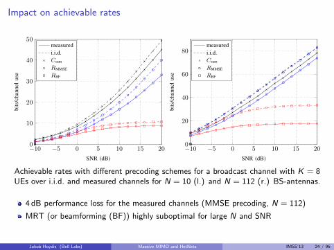
Impact on achievable rates

−10 −5 0 5 10 15 200

10

20

30

40

50

SNR (dB)

bits

/cha

nnel

use

measuredi.i.d.Csum

RMMSE

RBF

−10 −5 0 5 10 15 200

20

40

60

80

SNR (dB)

bits

/cha

nnel

use

measuredi.i.d.Csum

RMMSE

RBF

Achievable rates with different precoding schemes for a broadcast channel with K = 8UEs over i.i.d. and measured channels for N = 10 (l.) and N = 112 (r.) BS-antennas.

4 dB performance loss for the measured channels (MMSE precoding, N = 112)

MRT (or beamforming (BF)) highly suboptimal for large N and SNR


Lessons learned I

1 With very large antenna arrays, noise and interference vanish and the SNR can bemade inversely proportional to the number of antennas N without performance loss.This holds for the uplink and downlink.

2 The above conclusions hold with perfect CSI at the BS and under favorablepropagation characteristics, i.e., the channel vectors between to different UEsbecome orthogonal as N grows.

3 The channel orthogonality factors scales as 1/N for the i.i.d. model and as 1/N2 forpure LOS links.

4 Antenna correlation can have positive or negative effects depending on how UEs arescheduled. For a the one-ring model, the larger the angular separation between twoUEs, the more orthogonal the subspaces spanned by the correlation matrices.

5 Ray tracing and channel measurements show that we can expect favorablepropagation conditions in practice. However, the orthogonality scaling is slower thanpredicted by theory.

What happens if the channel must be estimated?What is the impact of hardware imperfections?


Outline





Channel estimation and the role of TDD

Channel knowledge at the BS is a must for precoding/beamforming and coherentdetection.

The channel coherence time fundamentally limits the number of BS-antennasand/or UEs:

I FDD: Downlink training + feedback as well as uplink training necessary

→Pilot overhead proportional to the number of antennas(unless certain channel conditions hold [8])

I TDD: Only uplink training needed

→Pilot overhead proportional to the number of UEs→We can add antennas at the BSs for “free” [11]

Remark

TDD relies on reciprocity of the uplink and downlink channels. While reciprocity holdswithout doubt for the physical propagation channel, it does not without calibration forthe transceiver RF chains. However, end-to-end reciprocity can be established bydifferent internal and external calibration mechanisms, as has been demonstrated inpractice (see, e.g., [12]).


Uplink channel training

The UEs transmit mutually orthogonal pilot sequences φi ∈ Cτ×1of length τ :

Y =(h1h2

)(φT1

φT2

)+ N

where Y,N ∈ CN×τand vec(N) ∼ CN (0, INτ ).

The BS correlates Y withφ?i‖φi‖2

:

Yφ?i‖φi‖2

= hi + ni

where ni ∼ CN (0, ‖φi‖−2IN).


Uplink channel training (cont.)

Let h1, h2 be independent and denote Ri4= E

[hih

Hi

]for i = 1, 2.

The BS calculates the linear MMSE estimate of hi based on Yφ?i‖φi‖2

:

hi = Ri

(Ri +

1

‖φi‖2IN

)−1

Yφ?i‖φi‖2

We can now decomposehi = hi + hi

where E[hi h

Hi

]= Ri

(Ri + 1

‖φi‖2 IN)−1

Ri4= Φi and E

[hi h

Hi

]= Ri −Φi .

Due to the orthogonality principle of the MMSE estimator, E[hHi hi

]= 0. If

hi ∼ CN (0,Ri ), then hi ∼ CN (0,Φi ) and hi ∼ CN (0,Ri −Φi ).

Assumptions for asymptotic considerations (as N → ∞):

tr Ri = ciN for some 0 < ci ≤ 1 (linear energy growth)

lim infN1N

rank(Ri ) > 0 (infinite degrees of freedom)

lim supN‖Ri‖ <∞ (finite energy per degree of freedom)


Achievable rates with imperfect CSI

During T − τ channel uses, the UEs transmit their data:

y(t) =2∑

i=1

hixi (t) + n(t) =2∑

i=1

(hi + hi

)xi (t) + n(t)

The BS estimates xi (t) after the projection of y(t) on hi . An achievable rate forUE 1 is given as [13]

R1 =(

1− τ

T

)E

log

1 +

‖h1‖4

hH1

(h2hH

2 + E[h1hH

1 |h1

]+ 1

SNRIN)

h1

For large N, we can find the following approximation:

R1 ≈(

1− τ

T

)log

1 +

(1N

tr Φ1

)2

1

N2tr Φ1R2

︸︷︷︸interference

+1

N2tr Φ1 (R1 −Φ1)

︸︷︷︸imperfect CSI

+1

NSNR

1

Ntr Φ1

︸︷︷︸noise


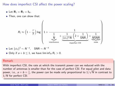
How does imperfect CSI affect the power scaling?

Let R1 = R2 = IN .

Then, one can show that:

R1 ≈(

1− τ

T

)log

1 +1

1

N︸︷︷︸interference

+1

‖φ1‖2N

(2 +

1

SNR

)

︸︷︷︸imperfect CSI

+1

NSNR︸︷︷︸noise

Let ‖φ1‖2 ∼ N−a, SNR ∼ N−b

Only if a + b ≤ 1, we have lim infN R1 > 0.

Remark

With imperfect CSI, the rate at which the transmit power can we reduced with thenumber of antennas is smaller than for the case of perfect CSI. For equal pilot and datapower, i.e., a = b = 1

2, the power can be made only proportional to 1/

√N in contrast to

1/N for perfect CSI.


Pilot contamination

The number of orthogonal pilot sequences is limited by the channel coherence time.Thus, the pilot sequences must be reused in neighboring cells.

Assume that both UEs transmit the same pilot sequence φ1 ∈ Cτ×1:

Y =(h1h2

)(φT1

φT1

)+ N

The BS correlates Y withφ?1‖φ1‖2

:

Yφ?1‖φ1‖2

= h1 + h2 + n1

...and calculates the linear MMSE estimate

h1 = R1

(R1 + R2 +

1

‖φ1‖2IN

)−1

︸︷︷︸4= S1

Yφ?1‖φ1‖2

E[h1hH

1

]4= Φ1 = R1

(R1 + R2 + 1

‖φ1‖2 IN)−1

R1 and E[h1hH

1

]= R1 −Φ1.

Remark

The channel estimate h1 is correlated with h2. This effect is called pilot contamination.


Achievable rate with pilot contamination

Similar to the case without pilot contamination, an achievable rate is given by

R1 =(

1− τ

T

)E

log

1 +

‖h1‖4

hH1

(h2hH

2 + E[h1hH

1

]+ 1

SNRIN)

h1

(N large)≈

(1− τ

T

)log (1 + γ1)

where

γ1 =

(1N

tr Φ1

)2

1

N2tr

(R1 +

1

‖φ1‖2IN

)SH

1 R2S1︸︷︷︸interference

+1

N2tr Φ1 (R1 −Φ1)︸︷︷︸imperfect CSI

+1

NSNR

1

Ntr Φ1︸︷︷︸

noise

+

∣∣∣∣ 1

Ntr S1R2

∣∣∣∣2︸︷︷︸pilot cont.

As N →∞,

limNγ1 = lim

N

(1N

tr Φ1

)2

∣∣∣∣ 1N

tr R1

(R1 + R2 + 1

‖φ1‖2 IN)−1

R2

∣∣∣∣2

(R1=R2=IN )= 1

Remark

As N →∞, pilot contamination can become a limiting factor.


When does pilot contamination become dominating?

0 20 40 60 80 100−200

−190

−180

−170

−160

−150

−140


Po

we

r (d

Bm

)

SignalInterferenceImperfect CSINoisePilot contamination

Powers of different parts of the received signal at the BS for Ri = d−3.6i IN with

d1 = 200 m, d2 = 500 m, and ‖φ‖2 = SNR = 121 dB.


What can we do against pilot contamination?

Correlation helps [14]: Let R1 = U1D1UH1 and R2 = U2D2UH

2 such thatUH

1 U2 = 0N . Then, R1 →∞ as N grows. Idea: Assign pilot sequences based onsecond-order channel statistics in order to reduce pilot contamination.

Blind or EVD-based channel estimation [15, 16]: Let Ri = βi IN for i = 1, 2 andassume β1 > β2. The BS observes the data transmissions during T time slots:

Y =(h1h2

)(x1(1) . . . x1(T )x2(1) . . . x2(T )

)+ N

where xi (t), ∀i , t, are i.i.d with zero mean and unit variance and Ni,j ∼ CN (0, 1).Let Y = [u1 . . . uN ] DVH. Then, as T ,N →∞, N/T → c and β1 >

√c,

1√N

uH1 h2

a.s.−−−−−→N,T→∞

0, | 1√N

uH1 h1|2

a.s.−−−−−→N,T→∞

β1.

Thus, the BS can detect x1(t) either blindly based on uH1 Y or estimate the effective

channel uH1 h1 from pilots without pilot contamination.

Other techniques: Pilot contamination precoding (multi-cell precoding based onchannel statistics and user data sharing) [17], Time-shifted pilots (UEs in differentcells transmit the pilots at different times) [18], many more...

Pilot contamination is not a fundamental limitation and can be efficiently mitigated!


What about FDD?

Channel estimation for the uplink is essentially the same as for TDD.

Estimating the downlink channel at the BS requires downlink training and feedbackfrom the UEs which is proportional to N.

Antenna correlation can be exploited to reduce this overhead!

Let the received signal at a UE be

y = hHwx + n

where w ∈ CN×1is a precoding vector, h ∼ CN (0,R), rank(R) = L, with SVD

R = UDUH and U ∈ CN×L.

Assuming that R is known, the BS can apply an “outer”-precoder U which reducesthe N-dimensional channel h to the L-dimensional effective channel UHh, i.e.,w = Uw, w ∈ CL×1

. The UE only estimates and feeds back the coefficients of theeffective channel. This overhead is proportional to L.

This idea can be extended to multiple UEs [8]: Group users with similar covariancematrices together, use MU-MIMO on the effective channel to separate the UEs of agroup, simultaneously schedule groups with almost orthogonal covariance matrices.The number of UEs per group is limited by the rank of the covariance matrix .


Joint Space-Division and Multiplexing (JSDM)

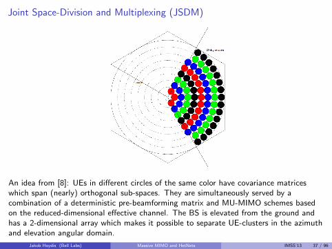
An idea from [8]: UEs in different circles of the same color have covariance matriceswhich span (nearly) orthogonal sub-spaces. They are simultaneously served by acombination of a deterministic pre-beamforming matrix and MU-MIMO schemes basedon the reduced-dimensional effective channel. The BS is elevated from the ground andhas a 2-dimensional array which makes it possible to separate UE-clusters in the azimuthand elevation angular domain.


Outline





Hardware impairments

Any transceiver suffers from hardware impairments whichI create a mismatch between the intended and emitted signalI distort the received signal

The distortions depend in general on the transmitted or received power.

Sources of impairments are:I oscillator phase noiseI amplifier non-linearity (especially for OFDM with high PAPR)I IQ imbalance due to imperfections in the quadrature mixerI quantization noise

Hardware impairments are known to limit the performance in the high-SNR regimebut much less is known for the large-N regime [19].

For massive MIMO cheap, low-power, and low-cost transceivers are desirable.

What are the impacts of hardware imperfections?

Can the hardware quality be reduced by increasing N?

All of the results in this part are taken from [20, 21] .


Uplink system and channel model

Downlink: Pilots & Data

Uplink: Pilots & Data

Base station User equipment

UplinkPilot & ControlSignals

Downlink DataTransmission

Coherence Period

Uplink DataTransmission

TULpilot TUL

data TDLpilot TDL

data

DownlinkPilot & ControlSignals

Tcoher

Uplink : yBS = h(

xUE + ηUEt

)+ ηBS

r + nBS

where E[∣∣xUE

∣∣2]

= pUE, nBS ∼ CN (0,S), and h ∼ CN (0,R).

Additive distortion

UE transmit distortion: ηUEt ∼ CN

(0, κUE

t pUE)

BS receive distortion: ηBSr ∼ CN (0, κBS

r pUEdiag(|h1|2, . . . , |hN |2))

The parameters κUEt and κBS

r are usually in the range [0, 0.03]. The smaller these values,the more accurate and expensive is the corresponding transceiver hardware component.


Channel estimation with hardware imperfections

The BSs computes the linear MMSE estimate of h based on a single uplink pilotxUE = d , |d |2 = pUE :

h = d?RZ−1yBS

where Rii is the ith diagonal element of R and

Z = E[yBS(yBS)H

]= pUE

(1 + κUE

t

)R + pUEκBS

r diag(R11, . . . ,RNN) + S.

We can decompose the channel as h = h + h, where

E[hhH

]= R− C

E[hhH

]= C

C = R− pUERZ−1R.

Remarks

Due to the distortion noise, the MMSE estimator is very complicated to derive andnot identical to the LMMSE estimator.

h and h are neither independent nor jointly complex Gaussian, but only uncorrelatedwith zero mean.


Channel estimation with hardware imperfections: Insights

Impact of pilot power

For R = S = IN , we have

C =

(1− 1

1 + κUEt + κBS

r + 1pUE

)IN , lim

pUE→∞C =

(1− 1

1 + κUEt + κBS

r

)IN .

Thus, even with infinite pilot power, perfect estimation accuracy cannot be achieved andthe performance is limited by the sum of the hardware impairments at the UE and BS.

Impact of pilot length

If the UE sends B pilot tones, the estimation accuracy can be improved by averaging Bseparate LMMSE estimates

h =1

B

B∑

i=1

hi = h− 1

B

B∑

i=1

hi .

If the errors hi are uncorrelated, they average out as B increases. However, the distortionmight be correlated and increasing B decreases the time for data transmission.


Channel estimation with hardware imperfections: Numerical results

0 5 10 15 20 25 30 35 4010−4

10−3

10−2

10−1

100

Average SNR [dB]

RelativeEstimationError

perA

nten

na

LMMSE EstimatorError Floors

κUEt =κBSr =0.152

κUEt =κBSr =0.12

κUEt =κBSr =0.052

κUEt =κBSr =0

Relative estimation error tr Ctr R

for N = 50 over SNR = pUE tr Rtr S

. The matrix R is generatedby the exponential model [22] with correlation coefficient ρ = 0.7 and S = IN .



1 2 3 4 5 6 7 8 9 1010

−4

10−3

10−2

10−1

100

Pilot Length (B )

Rel

ativ

e E

stim

atio

n E

rror

per

Ant

enna

Fully Correlated Distortion NoiseUncorrelated Distortion NoiseIdeal Hardware

5 dB

30 dB


over the pilot length B for for N = 50 and

κUEt = κBS

r = 0.052.



0 50 100 15010

−3

10−2

10−1

100

Number of Base Station Antennas (N )

Rel

ativ

e E

stim

atio

n E

rror

per

Ant

enna

Case 1: UncorrelatedCase 2: Exp.Mod., r = 0.7

Case 3: One-Ring, 20 degCase 4: One-Ring, 10 deg

5 dB

30 dB


over N for κUEt = κBS

r = 0.052.


Channel estimation with hardware imperfections: Discussion

Perfect channel estimation with hardware imperfections is impossible.

The estimation accuracy is fundamentally limited byI Distortions for high SNRI Coherence time and correlation of distortion noise for long pilot sequences

Hardware qualities of the UE and the BS are equally important.

The channel model largely impacts the estimation accuracy:Correlated channels are easier to estimate [23].

For large N, accurate estimates of R and S are difficult to obtain. The impact onthe estimation performance is unclear.

In practice [24], one would expect additive and multiplicative distortions. The latterare more difficult to analyze and can make things only worse.


Downlink channel model with hardware imperfections

Downlink: Pilots & Data

Uplink: Pilots & Data

Base station User equipment

UplinkPilot & ControlSignals

Downlink DataTransmission

Coherence Period

Uplink DataTransmission

TULpilot TUL

data TDLpilot TDL

data

DownlinkPilot & ControlSignals

Tcoher

Downlink : y UE = hH(

wxBS + ηBSt

)+ ηUE

r + nUE

where E[∣∣xBS

∣∣2]

= pUE, ‖w‖ = 1, and nUE ∼ CN (0, σ2UE).

Additive distortion

BS transmit distortion: ηBSt ∼ CN (0, κBS

t pBSdiag(|w1|2, . . . , |wN |2))

UE receive distortion: ηUEr ∼ CN (0, κUE

r pBS|hHw|)

Remark

Despite channel reciprocity, the UE needs to estimate the effective SISO channel hHw.


Capacity upper bounds

Assuming perfect CSI at the BS and UE and Gaussian signaling, one can show that theergodic UL and DL capacities are bounded from above by

CUL ≤TUL

data

TcoherE

log2

1 +hH(κBSr Dh + 1

pUE S)−1

h

1 + κUEt hH

(κBSr Dh + 1

pUE S)−1

h

≤ CULupper

4=

TULdata

Tcoherlog2

(1 +

GUL

1 + κUEt GUL

)

CDL ≤TDL

data

TcoherE

log2

1 +

hH

(κBSt Dh +

σ2UE

pBS I

)−1

h

1 + κUEr hH

(κBSt Dh +

σ2UE

pBS I

)−1

h

≤ CDLupper

4=

TDLdata

Tcoherlog2

(1 +

GDL

1 + κUEr GDL

)

where GUL = E[

hH(κBSr Dh + 1

pUE S)−1

h

], GDL = E

[hH

(κBSt Dh +

σ2UE

pBS I

)−1

h

], and

Dh = diag(|h1|2, . . . , |hN |2).


Asymptotic behavior of the upper bounds

High-SNR regime

limpUE→∞

C ULupper =

T ULdata

Tcoherlog2

(1 +

N

κBSr + NκUE

t

)

limpBS→∞

C DLupper =

T DLdata

Tcoherlog2

(1 +

N

κBSt + NκUE

r

)

Large-N regime

limN→∞

C ULupper =

T ULdata

Tcoherlog2

(1 +

1

κUEt

), lim

N→∞C DL

upper =T DL

data

Tcoherlog2

(1 +

1

κUEr

)

Observations

The UL/DL capacities have finite ceilings which depend on the hardware quality.

The UE impairments are N times more influential than the BS impairments.

As N →∞, only the UE hardware limits the performance; the BS distortionaverages out.


Capacity lower boundsOne can show that the ergodic UL/DL capacities are bounded from below by ([25, 13])

CUL ≥ CULlower =

TULdata

Tcoherlog2

(1 + SINRUL

lower

)CDL ≥ CDL

lower =TDL

data

Tcoherlog2

(1 + SINRDL

lower

)where vUL, vDL are functions of h and

SINRULlower =

∣∣E [hHvUL]∣∣2

(1 + κUEt )E

[∣∣hHvUL∣∣2]− ∣∣E [hHvUL

]∣∣2 + κBSr

∑Ni=1 E

[|hi |2|vUL

i |2]

+E[(vUL)HSvUL]

pUE

SINRDLlower =

∣∣E [hHvDL]∣∣2

(1 + κUEr )E

[∣∣hHvDL∣∣2]− ∣∣E [hHvDL

]∣∣2 + κBSt

∑Ni=1 E

[|hi |2|vDL

i |2]

+σ2

UEpBS

.

Remarks

The bounds hold for any vUL, vDL; especially for vUL = vDL = h‖h‖ .

CULlower depends only on κUE

t , κBSr while CDL

lower depends on all κ-parameters.

The impact of κBSt vanishes as N →∞.

One can show that, if κUEt = 0, limN→∞ CDL

upper − CDLlower = 0. This does not happen for

κBSr = 0. Thus, the capacity limit is mainly determined by the impairments at the UE.


Capacity bounds: Numerical results

0 100 200 300 400 5000

1

2

3

4

5

6

7

8


Spe

ctra

l Effi

cien

cy [b

its/c

hann

el u

se]

Capacity: Upper BoundsCapacity: Lower BoundsAsymptotic Limits (Upper & Lower)

κBS = κUT= 0.152

κBS = κUT= 0.052

κBS = κUT= 0

Lower and upper bounds on the capacity for R = S = I


Capacity bounds: Numerical results

0 200 400 600 800 10002

2.5

3

3.5

4


Spe

ctra

l Effi

cien

cy [b

its/c

hann

el u

se]

Capacity: Upper BoundsCapacity: Lower BoundsAsymptotic Limits (Upper & Lower)

κBS ∈ {0, 0.052, 0.152}

Decreasing withIncreasing

impairments:

Lower and upper bounds on the capacity for R = S = I and κUEt = κUE

r = 0.052. Theimpact of the hardware impairments at the BS vanishes asymptotically.


Scaling down the power or hardware quality

Uplink: Let pUE ∼ 1Nt , 0 < t < 1

2or κBS

r ∼ N t , 0 < t < 14. Then,

limN→∞

C UL ≥ log2

(1 +

1

2κUEt + (κUE

t )2

)

Downlink: Let pBS ∼ 1NtBS

, pUE ∼ 1NtUE

, tBS + tUE < 1, tBS ≥ 0, 0 < tUE <12

or

κBSr ∼ N t1 , κBS

t ∼ N t2 , 0 < t1 + t2 <12. Then,

limN→∞

C DL ≥ log2

(1 +

1

κUEr + κUE

t + κUEr κUE

t

)

Remark

The transmit powers can be roughly reduced as 1√N

or the hardware quality of the BS

transceiver can be reduced as 1√√N

while still a non-zero capacity is achieved.


Lessons learned II

With TDD, the pilot overhead is independent of N.

The effects of imperfect CSI vanish as N →∞.

The transmit power can be made proportional to 1/√

N when channel estimation istaken into account (in contrast to 1/N with perfect CSI). This holds even withhardware impairments.

Pilot contamination can be a performance bottleneck, but it is not a fundamentallimitation. It can be mitigated by blind channel estimation schemes, scheduling, orprecoding.

Hardware imperfections seem to be a fundamental limitation.

The quality of the UE-transceiver is more important than that of the BS-transceiver.

The quality of the BS-transceivers can be decreased as N grows (roughly

proportional to N−14 ).


Outline





Some interesting areas for future research

Channel modeling: Measurements, ray-tracing, new statistical models [26, 10]

New deployment models: Distributed massive MIMO, antennas in building facadesor windows [27], massive MIMO in HetNets [28, 29, 30]

New applications for massive MIMO: Wireless backhaul [31], sensor networks

Estimation of covariance matrices: Impact for channel estimation,precoding/detection

Hardware impairments: Fundamental limits and ways to mitigate them [20]

Cost and impacts of TDD reciprocity calibration

Combination of massive MIMO and stochastic geometry [32, 33]

Total energy efficiency of massive MIMO systems [34, 28, 20, 21]


Outline





Outline





Massive MIMO versus Small Cells

From a coverage as well as area spectral efficiency point of view, it is preferable todistribute the available antennas as much as possible [35].

However, with small cells deployed below the roof tops, it is difficult to

I ensure coverage

I support highly mobile UEs (due to frequent handovers)

But, massive MIMO is particularly suited to

I provide coverage of large areas

I support highly mobile UEs (TDD reduces the turnaround time)

Can we integrate the complementary benefits of both?


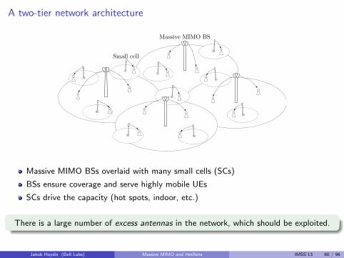
A two-tier network architecture

Massive MIMO BSs overlaid with many small cells (SCs)

BSs ensure coverage and serve highly mobile UEs

SCs drive the capacity (hot spots, indoor, etc.)

There is a large number of excess antennas in the network, which should be exploited.


The role of TDD

A network-wide synchronized TDD protocol has the following advantages:

The downlink channels can be estimated from uplink pilots.

→ Enable massive MIMO

Channel reciprocity holds for the desired and interfering channels.

→ Knowledge about the interfering channels can be acquired for freeat every device (BS, SC, UE).

Idea: “Sacrifice” excess antennas to reduce intra- and inter-tier interference.


Outline





A simple idea from cognitive radio [36]

1 The secondary BS listens to the transmission from the primary UE:

y = hx + n

2 ...and computes the covariance matrix of the receive signal:

E[yyH]

= hhH + SNR−1I



3 With the knowledge of the SNR, the secondary BS designs a precoder w which isorthogonal to the sub-space spanned by hhH.

4 The interference to the primary UE can be entirely eliminated without explicitknowledge of h.



3 With the knowledge of the SNR, the secondary BS designs a precoder w which isorthogonal to the sub-space spanned by hhH.

4 The interference to the primary UE can be entirely eliminated without explicitknowledge of h.


Outline





Translate this idea to HetNets

Every device estimates its received interference covariance matrix and precodes (partially)orthogonal to the dominating interference subspace.

Advantages

Interference to the directions from which a device received most interference isreduced.

No feedback or data exchange between the devices is needed.

Every device relies on locally available information alone.

The scheme is fully distributed an scalable.


Baseline scenarios: FDD, TDD, RTDD, and co-channel deployment

time

frequency

SC UL

SC DL

BS DL

BS UL

FDD TDD

SC DL

BS DL

SC UL

BS UL

time

frequency

co-channel TDD

SC DL

BS DL

SC UL

BS UL

time

frequency

co-channel reverse TDD

SC UL

BS DL

SC DL

BS UL

timefr

equency

FDD: Channel reciprocity does not hold

TDD: Only intra-tier interference can be reduced

co-channel TDD: Inter and intra-tier interference can be reduced

reverse (R) TDD: Order of UL/DL is reversed in one of the tiers


TDD versus reverse TDD (RTDD)

Order of UL/DL periods decides which devices interfere with each other:I TDD

F BS and small cell UEs (SUEs)F SCs and macro UEs (MUEs)F Intra-tier interference (SC-SUE, BS-MUE)

I RTDDF BS and SCsF MUEs and SUEsF Intra-tier interference (SC-SUE, BS-MUE)

The BS-SC channels change very slowly (quasi-static). Thus, covariance estimationbecomes easier for RTDD.


Co-channel TDD: Uplink signaling

BS i

SC i,s

MUE i,k

SUE i,s

N antennasF antennas single antenna

BS jMUE j,k

SC j,sSUE j,s

B BSs with N antennas

K single-ant. MUEs per BS

S SCs per BS with F antennas

1 single-ant. SUE per SC

Received signals at the ith BS and jth SC in cell i :

yBSi =

B∑

b=1

(K∑

k=1

√PMUEhBS-MUE

ibk xMUEbk +

S∑

s=1

√PSUEhBS-SUE

ibs xSUEbs

)+ nBS

i

y SCij =

B∑

b=1

(K∑

k=1

√PMUEhSC-MUE

ijbk xMUEbk +

S∑

s=1

√PSUEhSC-SUE

ijbs xSUEbs

)+ nSC

ij


Co-channel TDD: Uplink rates

BSs and SCs have perfect knowledge of the direct channels and the individualreceive covariance matrices:

QBSi = E

[yBSi (yBS

i )H], QSC

ij = E[y SCij (y SC

ij )H]

Achievable rates of the MUE k and SUE s in cell i with MMSE detection:

RUL,MUEik =

TUL

Tlog2

(1 + PMUE(hBS-MUE

iik )H(

QBSi − PMUEhBS-MUE

iik (hBS-MUEiik )H

)−1hBS-MUEiik

)RUL,SUEis =

TUL

Tlog2

(1 + PSUE(hSC-SUE

isis )H(

QSCis − PSUEhSC-SUE

isis (hSC-SUEisis )H

)−1hSC-SUEisis

)where T is the channel coherence time and TUL is the duration of the uplink cycle.

On the CSI assumption

In practice, the direct channels must be estimated by uplink pilots. For a sufficiently longcoherence time, the covariance matrices can be estimated by simple time averages. It isimplicitly assumed that the transmit powers and noise variances are perfectly known.


Co-channel TDD: Downlink signaling

Received signals at the jth MUE and jth SUE in cell i :

yMUEij =

B∑b=1

(K∑

k=1

√PBS

K(hBS-MUE

bij )HwBSbk x

BSbk +

S∑s=1

√PSC(hSC-MUE

bsij )HwSCbs x

SCbs

)+ nMUE

ij

ySUEij =

B∑b=1

(K∑

k=1

√PBS

K(hBS-SUE

bij )HwBSbk x

BSbk +

S∑s=1

√PSC(hSC-SUE

bsij )HwSCbs x

SCbs

)+ nSUE

ij

The BSs and SCs apply linear beamforming to serve their UEs:

wBSbk = κBS

bk

(1− α)PMUE

∑j

hBS-MUEbbj (hBS-MUE

bbj )H + αQBSb (1− α)No IN

−1

hBS-MUEbbk

wSCbs = κSC

bs

((1− β)PSUEhSC-SUE

bsbs (hSC-SUEbsbs )H + βQSC

bs + (1− β)No IF)−1

hSC-SUEbsbs

where α, β are regularization parameters and κBSbk , κ

SCbs normalize the vector norms to one.

About the regularization parameters

For α, β = 0, the BSs and SCs transmit as if they were in an isolated cell, i.e., MMSEprecoding (BSs) and maximum-ratio transmissions. By increasing α, β, the precodingvectors become increasingly orthogonal to the interference subspace.


Co-channel TDD: Downlink rates

Achievable downlink rates of the MUE k and SUE s in cell i :

RDL,MUEik =

(1−

TUL

T

)log2

(1 + SINRDL,MUE

ik

)RDL,SUEis =

(1−

TUL

T

)log2

(1 + SINRDL,SUE

is

)where

SINRDL,MUEik =

PBSK

∣∣(hBS-MUEiik )HwBS

ik

∣∣2No + PBS

K

∑(b,j)6=(i,k)

∣∣∣(hBS-MUEbik )HwBS

bj

∣∣∣2 + PSC∑

b,s

∣∣(hSC-MUEbsik )HwSC

bs

∣∣2SINRDL,SUE

is =PSC

∣∣(hSC-SUEisis )HwSC

is

∣∣2No + PBS

K

∑(b,j)

∣∣∣(hBS-SUEbis )HwBS

bj

∣∣∣2 + PSC∑

(b,s) 6=(i,s)

∣∣∣(hSC-SUEbjis )HwSC

bj

∣∣∣2

Other duplexing schemes

The other duplexing schemes work similarly, by adapting the covariance matrices and interferenceterms. In FDD, covariance knowledge cannot be exploited as channel reciprocity does not hold.Without co-channel deployment, there is only intra-tier interference.


Numerical results

1000 m

111 m

SC SUEMUEBS

40 m

3× 3 grid of BSs with wrap around

S = 81 SCs per cells on a regular grid

K = 20 MUEs randomly distributed ineach cell

1 SUE per SC randomly distributed ona disc around each SC

channel model with path loss,shadowing and fast fading, N/LOS linksfrom [37]

TX powers: 46 dBm (BS), 24 dBm(SC), 23 dBm (MUE/SUE)

20 MHz bandwidth, 2 GHz centerfrequency

no user scheduling, power control

averages over channel realizations andUE locations

TUL = 0.5T


Downlink rate regions

0 20 40 60 800

100

200

300

400

Macro DL area spectral efficiency(b/s/Hz/km2

)

SCD

Lar

easp

ectr

alef

ficie

ncy( b/

s/H

z/km

2) FDD (N = 20, F = 1)



0 20 40 60 800

100

200

300

400

FDD regionmore antennas

N = 20 → 100

F=

1→

4


)

SCD

Lar

easp

ectr

alef

ficie

ncy( b/

s/H

z/km

2) FDD (N = 20, F = 1)

FDD/TDD (N = 100, F = 4)



0 20 40 60 800

100

200

300

400

FDD region

TDD region

less intra-tier interf.α = 0 → 1

more antennasN = 20 → 100

F=

1→

4β

=0→

1


)

SCD

Lar

easp

ectr

alef

ficie

ncy( b/

s/H

z/km

2) FDD (N = 20, F = 1)

FDD/TDD (N = 100, F = 4)

TDD (N = 100, F = 4, α = 1, β = 1)



0 20 40 60 800

100

200

300

400

β

α

FDD region

TDD region

CoTDD region



F=

1→

4β

=0→

1


)

SCD

Lar

easp

ectr

alef

ficie

ncy( b/

s/H

z/km

2) FDD (N = 20, F = 1)

FDD/TDD (N = 100, F = 4)

TDD (N = 100, F = 4, α = 1, β = 1)



0 20 40 60 800

100

200

300

400

β

αβ

α

FDD region

TDD region

CoTDD region



F=

1→

4β

=0→

1

CoRTDD region


)

SCD

Lar

easp

ectr

alef

ficie

ncy( b/

s/H

z/km

2) FDD (N = 20, F = 1)

FDD/TDD (N = 100, F = 4)

TDD (N = 100, F = 4, α = 1, β = 1)


Uplink rate regions

0 20 40 60 800

100

200

300

400

α


F=

1→

4

Macro UL sum-rate(b/s/Hz/km2

)

Smal

lce

llU

Lsu

m-r

ate( b/

s/H

z/km

2)FDD/TDD (N = 20, F = 1)

FDD/TDD (N = 100, F = 4)

co-channel TDDco-channel reverse TDD


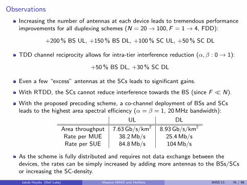
Observations

Increasing the number of antennas at each device leads to tremendous performanceimprovements for all duplexing schemes (N = 20→ 100,F = 1→ 4, FDD):

+200 % BS UL, +150 % BS DL, +100 % SC UL, +50 % SC DL

TDD channel reciprocity allows for intra-tier interference reduction (α, β : 0→ 1):

+50 % BS DL, +30 % SC DL

Even a few “excess” antennas at the SCs leads to significant gains.

With RTDD, the SCs cannot reduce interference towards the BS (since F � N).

With the proposed precoding scheme, a co-channel deployment of BSs and SCsleads to the highest area spectral efficiency (α = β = 1, 20 MHz bandwidth):

UL DL

Area throughput 7.63 Gb/s/km2 8.93 Gb/s/km2

Rate per MUE 38.2 Mb/s 25.4 Mb/sRate per SUE 84.8 Mb/s 104 Mb/s

As the scheme is fully distributed and requires not data exchange between thedevices, the rates can be simply increased by adding more antennas to the BSs/SCsor increasing the SC-density.


Discussion

Channel reciprocity requires:

I Hardware calibration [38, 39, 40, 12]I Scheduling of UEs on the same resource blocks in subsequent UL/DL cycles.

The network-wide TDD protocol requires tight synchronization of all devices:I GPS (outdoor)I NTP/PTP (indoor)I BS reference signals

Channel estimation will suffer from pilot contamination.

Covariance matrix estimation becomes difficult for large N,F [41, 42].

We have considered a worst case model with fixed cell association, no power controlor scheduling. Location-dependent user scheduling and interference-temperaturepower control could further enhance the performance [43].

Band switching duplexing could be used to reduce duplexing delays [44].


Outline





Outline





Massive MIMO for wireless backhaul

small cell

wireless backhaul

wireless datawired backhaul

user equipment

massive MIMO base station

Core network

The unrestrained SC-deployment “where needed” rather than “where possible”requires a high-capacity and easily accessible backhaul network.

Already for most WiFi deployments, the backhaul capacity (10–100 Mbit/s) and notthe air interface (54–600 Mbit/s) is the bottleneck.

Why not provide wireless backhaul with massive MIMO [31]?


Massive MIMO for wireless backhaul

small cell

wireless backhaul


user equipment


Core network

The unrestrained SC-deployment “where needed” rather than “where possible”requires a high-capacity and easily accessible backhaul network.

Already for most WiFi deployments, the backhaul capacity (10–100 Mbit/s) and notthe air interface (54–600 Mbit/s) is the bottleneck.

Why not provide wireless backhaul with massive MIMO [31]?


Massive MIMO wireless backhaul: Advantages

No standardization or backward-compatibility required

BS-SC channels change very slowly over time:

I Complex transmission/detection schemes (e.g., CoMP) can be easily implementedI FDD might be possible due to reduced CSI overhead

Provide backhaul where needed:

I Adapt backhaul capacity to the loadI Statistical multiplexing opportunity to avoid over-provisioning of backhaul

SCs require only a power connection to be operational

Line-of-sight not necessary if operated at low frequencies

Remark

Interestingly, the backhaul load is highest in lightly loaded cells where a single UE with avery good channel achieves the maximum possible data rate on the wireless link [45].


Massive MIMO wireless backhaul: Is it feasible?

How many antennas are needed to satisfy the desired backhaul rates with a giventransmit power budget?

Assumptions:

Every BS knows the channels to all SCs.

The BSs can exchange some control information.

Full user data sharing between the BSs is not possible.

Single-antenna SCs, BSs with N antennas

TDD with channel reciprocity

Check if the power minimization problem with target SINR constraints for the multi-cellmulti-antenna wireless system is feasible [46].


Outline





The multi-cell multi-antenna power minimization and beamforming problem

P 1: Power minimization problem [46]

min∑

bs

wHbswbs

s.t. SINRbs ≥ γbs 1 ≤ b ≤ B, 1 ≤ s ≤ S

wbs is the beamforming vector of BS b towards SC s in its cell

γbs is the target SINR of the backhaul link to SC s in cell b

SINRbs is the SINR of the backhaul link to SC s in cell b:

SINRbs =

∣∣wHbshbbs

∣∣2∑

l 6=s

∣∣wHblhbbs

∣∣2 +∑

m 6=b,l

∣∣wHmlhmbs

∣∣2 + No

where hmbs ∈ CN×1is the channel from BS m to SC s in cell b.

Remark

The problem is always feasible if N ≥ B × S since zero-forcing can be applied.


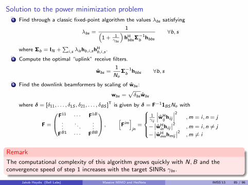
Solution to the power minimization problem1 Find through a classic fixed-point algorithm the values λbs satisfying

λbs =1(

1 + 1γbs

)hHbbsΣ−1

b hbbs

∀b, s

where Σb = IN +∑

i,s λishb,i,shHb,i,s .

2 Compute the optimal “uplink” receive filters.

wbs =1

NoΣ−1

b hbbs ∀b, s

3 Find the downlink beamformers by scaling of wbs :

wbs =√δbs wbs

where δ = [δ11, . . . , δ1S , δ21, . . . , δBS ]T is given by δ = F−11BSNo with

F =

F11 · · · F1B

.... . .

...FB1 · · · FBB

,[Fim]jn

=

1γij

∣∣∣wHij hiij

∣∣∣2 ,m = i , n = j

−∣∣wH

inhiij

∣∣2 ,m = i , n 6= j

−∣∣wH

mnhmij

∣∣2 ,m 6= i

Remark

The computational complexity of this algorithm grows quickly with N,B and theconvergence speed of step 1 increases with the target SINRs γbs .


“Antenna” minimization problem

P 2: Minimization of N

min N

s.t.1

B

∑

b,s

wHbswbs ≤ PBS

where wbs are given by the solution of the power minimization problem P 1.

Solution of P 1 becomes prohibitive for large N, S : Large system approximation [47]I computed based on the second-order statistics of the channelsI complexity is independent of NI solution is asymptotically optimal (for N, S →∞)

By UL/DL duality, the same target DL SINRs γbs can be achieved in the UL withthe receive filters wbs at the BSs and the SC transmit powers λbs . However, theindividual power budgets of the SCs are not respected in this case.

Numerical results based on the 3× 3 macro-cell setup as described earlier. Thedownlink TDD cycle is twice as long as the uplink cycle.


Massive MIMO backhaul: Numerical results

0 20 40 60 80 1000

100

200

300

400

500

Downlink backhaul rate (Mbit/s)

Req

uire

d#

ofB

S-an

tenn

as

S = 81

S = 40

S = 20

0 10 20 30 40 50Uplink backhaul rate (Mbit/s)

Average minimum number of required BS-antennas N to serve S ∈ {20, 40, 81} randomlychosen SCs with the same target backhaul rate and with 46 dBm maximum averagetransmit power per BS.


Massive MIMO backhaul: Numerical results

0 20 40 60 80 10020

30

40

46

50

Downlink backhaul rate (Mbit/s)

Min

imum

tran

smit

pow

erpe

rB

S(d

Bm

) S = 81

S = 40

S = 20

0 10 20 30 40 50Uplink backhaul rate (Mbit/s)

Minimum average required transmit power per BS to serve S ∈ {20, 40, 81} randomlychosen SCs with the same target backhaul rate and the smallest possible number ofBS-antennas N.


Discussion

small cell

wireless backhaul

cache


user equipment


Core network

Is there an advantage to serve UEs via SCs rather than directly by the BSs?

I Long coherence time of the BS-SC channels enables complex precoding schemes.

I Uplink transmit power can be drastically reduced.

I SCs with wireless backhaul are essentially relays which can cover hidden areas.

Low frequencies are suited for (NLOS) backhaul (small propagation losses) whilehigher frequencies are suited for SCs to reduce interference.

Given enough BS-antennas, even in-band backhaul could be provided.

SCs could preload popular files on integrated hard discs [48] based on learning andprediction algorithms to reduce the backhaul bandwidth.


Discussion

small cell

wireless backhaul

cache


user equipment


Core network

Is there an advantage to serve UEs via SCs rather than directly by the BSs?

I Long coherence time of the BS-SC channels enables complex precoding schemes.

I Uplink transmit power can be drastically reduced.

I SCs with wireless backhaul are essentially relays which can cover hidden areas.

Low frequencies are suited for (NLOS) backhaul (small propagation losses) whilehigher frequencies are suited for SCs to reduce interference.

Given enough BS-antennas, even in-band backhaul could be provided.

SCs could preload popular files on integrated hard discs [48] based on learning andprediction algorithms to reduce the backhaul bandwidth.


Lessons learned III

Massive MIMO and SCs have distinct advantages which complement each other:

I Massive MIMO for area coverage and mobility supportI SCs for capacity and indoor coverage

TDD and the resulting channel reciprocity allows every device to fully exploit itsavailable degrees of freedom for intra-/inter-tier interference mitigation.

A co-channel deployment of massive MIMO BSs and SCs can achieve a veryattractive rate region.

Massive MIMO BSs can provide wireless backhaul to a large number of SCs:With N = 466 antennas per BS, it is possible to provide 81 SCs with 100 Mb/s(DL)/ 50 Mb/s (UL) backhaul.


Thank you!


References I

[1] J. Hoydis, S. ten Brink, and M. Debbah, “Massive MIMO in the UL/DL of cellular networks: How many antennas do weneed?” IEEE J. Sel. Areas Commun., vol. 31, no. 2, pp. 160–171, Feb. 2013.

[2] T. L. Marzetta, “Noncooperative cellular wireless with unlimited numbers of base station antennas,” IEEE Trans. WirelessCommun., vol. 9, no. 11, pp. 3590–3600, Nov. 2010.

[3] F. Rusek, D. Persson, B. K. Lau, E. G. Larsson, T. L. Marzetta, O. Edfors, and F. Tufvesson, “Scaling up MIMO:Opportunities and challenges with very large arrays,” IEEE Signal Process. Mag., vol. 30, no. 1, pp. 40–46, Jan. 2013.

[4] D. Tse and P. Viswanath, Fundamentals of Wireless Communications. New York, NY, USA: Cambridge University Press,2005.

[5] Z. D. Bai and J. W. Silverstein, Spectral Analysis of Large Dimensional Random Matrices, 2nd ed. Springer Series inStatistics, New York, NY, USA, 2009.

[6] R. Couillet and M. Debbah, Random matrix methods for wireless communications, 1st ed. New York, NY, USA:Cambridge University Press, 2011.

[7] D. Shiu, G. J. Foschini, M. J. Gans, and J. M. Kahn, “Fading correlation and its effect on the capacity of multielementantenna systems,” IEEE Trans. Commun., vol. 48, no. 3, pp. 502–513, Mar. 2000.

[8] A. Adhikary, J. Nam, J.-Y. Ahn, and G. Caire, “Joint spatial division and multiplexing,” 2012, submitted. [Online].Available: http://arxiv.org/abs/1209.1402

[9] S. J. Fortune, D. M. Gay, B. W. Kernighan, O. Landron, R. A. Valenzuela, and M. H. Wright, “WISE design of indoorwireless systems: practical computation and optimization,” IEEE Computational Science Engineering, vol. 2, no. 1, pp.58–68, Spring 1995.

[10] J. Hoydis, C. Hoek, T. Wild, and S. ten Brink, “Channel measurements for large antenna arrays,” in Proc. IEEEInternational Symposium on Wireless Communication Systems (ISWCS), Paris, France, Aug. 2012, pp. 811–815.

[11] T. L. Marzetta, “How much training is required for multiuser MIMO?” in Proc. IEEE Asilomar Conference on Signals,Systems and Computers (ACSSC), Pacific Grove, CA, US, Nov. 2006, pp. 359–363.


http://arxiv.org/abs/1209.1402

References II

[12] C. Shepard, H. Yu, N. Anand, L. E. Li, T. L. Marzetta, R. Yang, and L. Zhong, “Argos: Practical many-antenna basestations,” in Proc. ACM Int. Conf. Mobile Computing and Networking (MobiCom), Istanbul, Turkey, Aug. 2012, pp. 53–64.

[13] B. Hassibi and B. M. Hochwald, “How much training is needed in multiple-antenna wireless links?” IEEE Trans. Inf.Theory, vol. 49, no. 4, pp. 951–963, Apr. 2003.

[14] H. Yin, D. Gesbert, M. Filippou, and L. Yingzhuang, “A coordinated approach to channel estimation in large-scalemultiple-antenna systems,” IEEE J. Sel. Areas Commun., vol. 31, no. 2, pp. 264–273, Feb. 2013.

[15] R. Muller, M. Vehkapera, and L. Cottatellucci, “Blind pilot decontamination,” Proc. 17 th Intl ITG Workshop on SmartAntennas (WSA), Mar. 2013.

[16] H. Q. Ngo and E. G. Larsson, “EVD-based channel estimation in multicell multiuser MIMO systems with very large antennaarrays,” in IEEE International Conference on Acoustics, Speech and Signal Processing (ICASSP, Kyoto, Japan, Mar. 2012,pp. 3249–3252.

[17] A. Ashikhmin and T. L. Marzetta, “Pilot contamination precoding in multi-cell large scale antenna systems,” in IEEEInternational Symposium on Information Theory (ISIT), Cambridge, MA, USA, Jul. 2012, pp. 1137–1141.

[18] F. Fernandes, A. Ashikhmin, and T. Marzetta, “Inter-cell interference in noncooperative TDD large scale antenna systems,”IEEE J. Sel. Areas Commun., vol. 31, no. 2, pp. 192–201, Feb. 2013.

[19] A. Pitarokoilis, S. K. Mohammed, and E. G. Larsson, “Effect of oscillator phase noise on uplink performance of largeMU-MIMO systems,” in Proc. 50th Annual Allerton Conference onCommunication, Control, and Computing (Allerton),Urbana-Champaign, IL, USA, Oct. 2012, pp. 1190–1197.

[20] E. Bjornson, J. Hoydis, M. Kountouris, and M. Debbah, “Hardware impairments in large-scale MISO systems: Energyefficiency, estimation, and capacity limits,” in Proc. International Conference on Signal Processing (DSP): Special Sessionon Signal Processing and Optimization for Green Energy and Green Communications, Santorini, Greece, Jul. 2013. [Online].Available: http://arxiv.org/abs/1305.4651

[21] ——, “Massive MIMO systems with non-ideal hardware: Energy efficiency, estimation, and capacity limits,” 2013, inpreparation.



References III

[22] S. L. Loyka, “Channel capacity of MIMO architecture using the exponential correlation matrix,” IEEE Commun. Lett.,vol. 5, no. 9, pp. 369–371, Sep. 2001.

[23] E. Bjornson and B. Ottersten, “A framework for training-based estimation in arbitrarily correlated Rician MIMO channelswith Rician disturbance,” IEEE Trans. Signal Process., vol. 58, no. 3, pp. 1807–1820, Mar. 2010.

[24] J. J. Bussgang, “Crosscorrelation functions of amplitude-distorted gaussian signals,” Research Laboratory of Electronics,Massachusetts Institute of Technology, Tech. Rep. 216, 1952.

[25] M. Medard, “The effect upon channel capacity in wireless communications of perfect and imperfect knowledge of thechannel,” IEEE Trans. Inf. Theory, vol. 46, no. 3, pp. 933–946, May 2000.

[26] S. Payami and F. Tufvesson, “Channel measurements and analysis for very large array systems at 2.6 Ghz,” in Proc. 6thEuropean Conference on Antennas and Propagation (EuCAP), Prague, Czech Republic, Mar. 2012, pp. 433–437.

[27] “Window of opportunity,” http://www.ericsson.com/thinkingahead/networked society/window of opportunity, accessed:2013-05-17.

[28] E. Bjornson, M. Kountouris, and M. Debbah, “Massive MIMO and small cells: Improving energy efficiency by optimalsoft-cell coordination,” in International Conference on Telecommunications (ICT), Casablanca, Morocco, May 2013.

[29] J. Hoydis, K. Hosseini, S. ten Brink, and M. Debbah, “Making smart use of excess antennas: Massive MIMO, small cells,and TDD,” Bell Labs Technical Journal, vol. 18, no. 2, Sep. 2013.

[30] “Massive MIMO and small cells: How to densify heterogeneous networks,” in IEEE International Conference onCommunications (ICC), Budapest, Hungary, Jun. 2013.

[31] T. L. Marzetta and H. Yang, “Dedicated LSAS for metro-cell wireless backhaul - Part I: Downlink,” Bell Laboratories,Alcatel-Lucent, Tech. Rep., Dec. 2012.

[32] T. Bai and R. W. Heath, “Asymptotic coverage probability and rate in massive MIMO networks,” 2013, submitted. [Online].Available: http://arxiv.org/abs/1305.2233


http://www.ericsson.com/thinkingahead/networked_society/window_of_opportunity


References IV

[33] J. Hoydis, A. Muller, R. Couillet, and M. Debbah, “Analysis of multicell cooperation with random user locations viadeterministic equivalents,” in IEEE International Symposium on Modeling and Optimization in Mobile, Ad Hoc and WirelessNetworks (WiOpt): Workshop on Spatial Stochastic Models for Wireless Networks (SPASWIN), Paderborn, Germany, May2012, pp. 374–379.

[34] H. Q. Ngo, E. G. Larsson, and T. L. Marzetta, “Energy and spectral efficiency of very large multiuser MIMO systems,” IEEETrans. Commun., vol. 4, no. 61, pp. 1436–1449, Apr. 2013.

[35] H. S. Dhillon, M. Kountouris, and J. G. Andrews, “Downlink MIMO hetnets: Modeling, ordering results and performanceanalysis,” IEEE Trans. Wireless Commun., 2013, submitted. [Online]. Available: http://arxiv.org/abs/1301.5034

[36] R. Zhang, F. Gao, and Y.-C. Liang, “Cognitive beamforming made practical: Effective interference channel andlearning-throughput tradeoff,” IEEE Trans. Commun., vol. 58, no. 2, pp. 706–718, Feb. 2010.

[37] 3rd Generation Partnership Project, “Technical Specification Group Radio Access Network, Evolved Universal TerrestrialRadio Access (E-UTRA), Further Enhancements to LTE Time Division Duplex (TDD) for Downlink-Uplink (DL-UL)Interference Management and Traffic Adaptation (Release 11), 3GPP TR 36.828, v11.0.0,” Jun. 2012. [Online]. Available:http://www.3gpp.org/ftp/Specs/html-info/36828.htm

[38] J.-C. Guey and L. D. Larsson, “Modeling and evaluation of MIMO systems exploiting channel reciprocity in TDD mode,” inIEEE Vehicular Technology Conference (VTC Fall), Los Angeles, CA, USA, Sep. 2004, pp. 4265–4269.

[39] M. Guillaud, D. T. M. Slock, and R. Knopp, “A practical method for wireless channel reciprocity exploitation throughrelative calibration,” in IEEE International Symposium on Signal Processing and Its Applications (ISSPA), Sydney, Australia,Aug. 2005, pp. 403–406.

[40] J. Shi, Q. Luo, and M. You, “An efficient method for enhancing TDD over the air reciprocity calibration,” in IEEE WirelessCommunication and Networking Conference (WCNC), Cancun, Mexico, Mar. 2011, pp. 339–344.

[41] R. Couillet and M. Debbah, “Signal processing in large systems: A new paradigm,” IEEE Signal Process. Mag., vol. 30, pp.24–39, Jan. 2013.

[42] O. Ledoit and M. Wolf, “A well-conditioned estimator for large-dimensional covariance matrices,” J. Multivariate Anal,vol. 88, p. 365411, Feb. 2004.



http://www.3gpp.org/ftp/Specs/html-info/36828.htm

References V

[43] A. Adhikary and G. Caire, “On the coexistence of macrocell spatial multiplexing and cognitive femtocells,” in IEEEInternational Conference on Communications (ICC), Ottawa, Canada, Jun. 2012, pp. 6830–6834.

[44] P. Bosch and S. J. Mullender, “Band switching for coherent beam forming in full-duplex wireless communication,” U.S.Patent 2005/0 243 748 A1, 2005. [Online]. Available: http://www.freepatentsonline.com/y2005/0243748.html

[45] Small Cell Forum, “Release One, Document 049.01.01, Backhaul technologies for small cells,” Feb. 2013. [Online].Available: http://scf.io/en/documents/049 Backhaul technologies for small cells.php

[46] H. Dahrouj and W. Yu, “Coordinated beamforming for the multicell multi-antenna wireless system,” IEEE Trans. WirelessCommun., vol. 9, no. 5, pp. 1748–1759, May 2010.

[47] S. Lakshminarayana, J. Hoydis, M. Debbah, and M. Assaad, “Asymptotic analysis of distributed multi-cell beamforming,” inIEEE International Symposium in Personal Indoor and Mobile Radio Communications (PIMRC), Istanbul, Turkey, Sep. 2010,pp. 2105–2110.

[48] N. Golrezaei, K. Shanmugam, A. Dimakis, A. F. Molisch, and G. Caire, “Femtocaching: Wireless video content deliverythrough distributed caching helpers,” in IEEE International Conference on Computer Communications, Orlando, Florida,USA, Mar. 2012, pp. 1107–1115.


http://www.freepatentsonline.com/y2005/0243748.html

http://scf.io/en/documents/049_Backhaul_technologies_for_small_cells.php

Documents

Massive MIMO and HetNets: Benefits and Challengeseuracon.org/attached/Hoydis - Massive MIMO and... · Massive MIMO and HetNets: Bene ts and Challenges Jakob Hoydis Bell Laboratories,