Embed Size (px)
Citation preview

Reproductive Health Research Analysis Software (RHAS) v1.1USER GUIDE
Publication Number 703517
Revision 2
For Research Use Only. Not for use in diagnostic procedures.

Affymetrix, Inc.3450 Central ExpresswaySanta Clara, CA 95051
The information in this guide is subject to change without notice.
DISCLAIMER
TO THE EXTENT ALLOWED BY LAW, LIFE TECHNOLOGIES AND/OR ITS AFFILIATE(S) WILL NOT BE LIABLE FOR SPECIAL, INCIDENTAL, INDIRECT, PUNITIVE, MULTIPLE, OR CONSEQUENTIAL DAMAGES IN CONNECTION WITH OR ARISING FROM THIS DOCUMENT, INCLUDING YOUR USE OF IT.
Revision history: Pub No. 703517
Important Software Licensing Information
Your installation and/or use of this Reproductive Health Research Analysis software is subject to the terms and conditions contained in the End User License Agreement (EULA) which is incorporated within the Reproductive Health Research Analysis software, and you will be bound by the EULA terms and conditions if you install and/or use the software.
NOTICE TO PURCHASER: DISCLAIMER OF LICENSE
Purchase of this software product alone does not imply any license under any process, instrument or other apparatus, system, composition, reagent or kit rights under patent claims owned or otherwise controlled by Life Technologies Corporation, either expressly, or by estoppel.
Legal entity
Affymetrix, Inc. | Santa Clara, CA 95051 USA | Toll Free in USA 1 800 955 6288
TRADEMARKS
All trademarks are the property of Thermo Fisher Scientific and its subsidiaries unless otherwise specified.
©2021 Thermo Fisher Scientific Inc. All rights reserved.
Revision Date Description 2 October 2021 Added Mendelian Error Checking 1 February 2020 Initial release

Contents
CHAPTER 1 Installation and setup . . . . . . . . . . . . . . . . . . . . . . . . . . . . . . 9
Introduction . . . . . . . . . . . . . . . . . . . . . . . . . . . . . . . . . . . . . . . . . . . . . . . . . . . . . . . . . . . . . . . . . . . .9
RHAS workflow . . . . . . . . . . . . . . . . . . . . . . . . . . . . . . . . . . . . . . . . . . . . . . . . . . . . . . . . . . . . . . . . .10
System requirements . . . . . . . . . . . . . . . . . . . . . . . . . . . . . . . . . . . . . . . . . . . . . . . . . . . . . . . . . . .11Recommended hardware . . . . . . . . . . . . . . . . . . . . . . . . . . . . . . . . . . . . . . . . . . . . . . . . . . . . . .11
Minimum requirements . . . . . . . . . . . . . . . . . . . . . . . . . . . . . . . . . . . . . . . . . . . . . . . . . . . . . . . .11
Preferences . . . . . . . . . . . . . . . . . . . . . . . . . . . . . . . . . . . . . . . . . . . . . . . . . . . . . . . . . . . . . . . . . . .13Assigning a library folder/path . . . . . . . . . . . . . . . . . . . . . . . . . . . . . . . . . . . . . . . . . . . . . . . . . 14
Downloading library files . . . . . . . . . . . . . . . . . . . . . . . . . . . . . . . . . . . . . . . . . . . . . . . . . . . . . . .14
Setting up custom proxy settings . . . . . . . . . . . . . . . . . . . . . . . . . . . . . . . . . . . . . . . . . . . . . . . .15
CHAPTER 2 Performing an analysis . . . . . . . . . . . . . . . . . . . . . . . . . . . . 16
Importing CEL files . . . . . . . . . . . . . . . . . . . . . . . . . . . . . . . . . . . . . . . . . . . . . . . . . . . . . . . . . . . . .16
Adding columns (optional) . . . . . . . . . . . . . . . . . . . . . . . . . . . . . . . . . . . . . . . . . . . . . . . . . . . . . . . .17
Importing sample attributes . . . . . . . . . . . . . . . . . . . . . . . . . . . . . . . . . . . . . . . . . . . . . . . . . . . . . .17
Saving attributes (optional) . . . . . . . . . . . . . . . . . . . . . . . . . . . . . . . . . . . . . . . . . . . . . . . . . . . . . . .18
Saving attributes as a TXT file . . . . . . . . . . . . . . . . . . . . . . . . . . . . . . . . . . . . . . . . . . . . . . . . . . .18
Saving attributes as ARR files . . . . . . . . . . . . . . . . . . . . . . . . . . . . . . . . . . . . . . . . . . . . . . . . . . .18
Copying selected rows . . . . . . . . . . . . . . . . . . . . . . . . . . . . . . . . . . . . . . . . . . . . . . . . . . . . . . . . . . .18
Sorting columns . . . . . . . . . . . . . . . . . . . . . . . . . . . . . . . . . . . . . . . . . . . . . . . . . . . . . . . . . . . . . . . .18
Removing CEL files . . . . . . . . . . . . . . . . . . . . . . . . . . . . . . . . . . . . . . . . . . . . . . . . . . . . . . . . . . . . .19
Configuring your files for analysis . . . . . . . . . . . . . . . . . . . . . . . . . . . . . . . . . . . . . . . . . . . . . . . . .19
Using the analysis configuration window . . . . . . . . . . . . . . . . . . . . . . . . . . . . . . . . . . . . . . . . . .20
Copy number options . . . . . . . . . . . . . . . . . . . . . . . . . . . . . . . . . . . . . . . . . . . . . . . . . . . . . . . . . . . .20
Analysis . . . . . . . . . . . . . . . . . . . . . . . . . . . . . . . . . . . . . . . . . . . . . . . . . . . . . . . . . . . . . . . . . . . . .20
Analysis pane options . . . . . . . . . . . . . . . . . . . . . . . . . . . . . . . . . . . . . . . . . . . . . . . . . . . . . . . . .20
Thresholds . . . . . . . . . . . . . . . . . . . . . . . . . . . . . . . . . . . . . . . . . . . . . . . . . . . . . . . . . . . . . . . . . .21
SMN reporting . . . . . . . . . . . . . . . . . . . . . . . . . . . . . . . . . . . . . . . . . . . . . . . . . . . . . . . . . . . . . . . . .21
Genotyping options . . . . . . . . . . . . . . . . . . . . . . . . . . . . . . . . . . . . . . . . . . . . . . . . . . . . . . . . . . . . . .21
Thresholds . . . . . . . . . . . . . . . . . . . . . . . . . . . . . . . . . . . . . . . . . . . . . . . . . . . . . . . . . . . . . . . . . .21
Genotyping QC . . . . . . . . . . . . . . . . . . . . . . . . . . . . . . . . . . . . . . . . . . . . . . . . . . . . . . . . . . . . . . .22
Genotyping analysis . . . . . . . . . . . . . . . . . . . . . . . . . . . . . . . . . . . . . . . . . . . . . . . . . . . . . . . . . . .22
Carrier reporting . . . . . . . . . . . . . . . . . . . . . . . . . . . . . . . . . . . . . . . . . . . . . . . . . . . . . . . . . . . . .22
Optional parameters . . . . . . . . . . . . . . . . . . . . . . . . . . . . . . . . . . . . . . . . . . . . . . . . . . . . . . . . . .23
Advanced genotyping options . . . . . . . . . . . . . . . . . . . . . . . . . . . . . . . . . . . . . . . . . . . . . . . . . . .23
SNP metrics options . . . . . . . . . . . . . . . . . . . . . . . . . . . . . . . . . . . . . . . . . . . . . . . . . . . . . . . . . . . .23
Configuring your analysis . . . . . . . . . . . . . . . . . . . . . . . . . . . . . . . . . . . . . . . . . . . . . . . . . . . . . . . .24
Selecting an array type . . . . . . . . . . . . . . . . . . . . . . . . . . . . . . . . . . . . . . . . . . . . . . . . . . . . . . . .24
Selecting a workflow . . . . . . . . . . . . . . . . . . . . . . . . . . . . . . . . . . . . . . . . . . . . . . . . . . . . . . . . . .24
RHAS User Guide 3

Contents
Assigning a result name. . . . . . . . . . . . . . . . . . . . . . . . . . . . . . . . . . . . . . . . . . . . . . . . . . . . . . . 25
Assigning a result suffix (optional) . . . . . . . . . . . . . . . . . . . . . . . . . . . . . . . . . . . . . . . . . . . . . . .25
Assigning an output folder path . . . . . . . . . . . . . . . . . . . . . . . . . . . . . . . . . . . . . . . . . . . . . . . . .25
Adding sub-folders . . . . . . . . . . . . . . . . . . . . . . . . . . . . . . . . . . . . . . . . . . . . . . . . . . . . . . . . .25Running your analysis . . . . . . . . . . . . . . . . . . . . . . . . . . . . . . . . . . . . . . . . . . . . . . . . . . . . . . . . . . .26
CHAPTER 3 Dashboard. . . . . . . . . . . . . . . . . . . . . . . . . . . . . . . . . . . . . . . 27
Overview . . . . . . . . . . . . . . . . . . . . . . . . . . . . . . . . . . . . . . . . . . . . . . . . . . . . . . . . . . . . . . . . . . . . . .27
Dashboard warning messages . . . . . . . . . . . . . . . . . . . . . . . . . . . . . . . . . . . . . . . . . . . . . . . . . . . .27
Viewing the message . . . . . . . . . . . . . . . . . . . . . . . . . . . . . . . . . . . . . . . . . . . . . . . . . . . . . . . .27Common warnings . . . . . . . . . . . . . . . . . . . . . . . . . . . . . . . . . . . . . . . . . . . . . . . . . . . . . . . . . .28
Using the dashboard . . . . . . . . . . . . . . . . . . . . . . . . . . . . . . . . . . . . . . . . . . . . . . . . . . . . . . . . . . . .28
Opening a selected result . . . . . . . . . . . . . . . . . . . . . . . . . . . . . . . . . . . . . . . . . . . . . . . . . . . . . .28
Searching for a completed analysis . . . . . . . . . . . . . . . . . . . . . . . . . . . . . . . . . . . . . . . . . . . . . .28
Browsing for an existing result . . . . . . . . . . . . . . . . . . . . . . . . . . . . . . . . . . . . . . . . . . . . . . . . . .28
Removing a selected result . . . . . . . . . . . . . . . . . . . . . . . . . . . . . . . . . . . . . . . . . . . . . . . . . . . . .28
CHAPTER 4 MSV setup and features. . . . . . . . . . . . . . . . . . . . . . . . . . . . 29
Overview . . . . . . . . . . . . . . . . . . . . . . . . . . . . . . . . . . . . . . . . . . . . . . . . . . . . . . . . . . . . . . . . . . . . . .29
Supported data types . . . . . . . . . . . . . . . . . . . . . . . . . . . . . . . . . . . . . . . . . . . . . . . . . . . . . . . . . . . .29
Launching the MSV . . . . . . . . . . . . . . . . . . . . . . . . . . . . . . . . . . . . . . . . . . . . . . . . . . . . . . . . . . . . .29
MSV tool bar . . . . . . . . . . . . . . . . . . . . . . . . . . . . . . . . . . . . . . . . . . . . . . . . . . . . . . . . . . . . . . . . . . .30
Synchronizing MSV and ChAS . . . . . . . . . . . . . . . . . . . . . . . . . . . . . . . . . . . . . . . . . . . . . . . . . . . . .30
MSV preferences without ChAS synchronization . . . . . . . . . . . . . . . . . . . . . . . . . . . . . . . . . . . . .31
General window tab . . . . . . . . . . . . . . . . . . . . . . . . . . . . . . . . . . . . . . . . . . . . . . . . . . . . . . . . . . .31
Choosing a library folder location . . . . . . . . . . . . . . . . . . . . . . . . . . . . . . . . . . . . . . . . . . . . .31Setting up stand-alone preferences in MSV . . . . . . . . . . . . . . . . . . . . . . . . . . . . . . . . . . . . .31Managing Library Files . . . . . . . . . . . . . . . . . . . . . . . . . . . . . . . . . . . . . . . . . . . . . . . . . . . . . .31Proxy settings . . . . . . . . . . . . . . . . . . . . . . . . . . . . . . . . . . . . . . . . . . . . . . . . . . . . . . . . . . . . . .31
Smoothing and joining settings window tab . . . . . . . . . . . . . . . . . . . . . . . . . . . . . . . . . . . . . . . 32
Editing the Smoothing/Joining settings . . . . . . . . . . . . . . . . . . . . . . . . . . . . . . . . . . . . . . . . .32Segment filter settings window tab. . . . . . . . . . . . . . . . . . . . . . . . . . . . . . . . . . . . . . . . . . . . . . 34
Setting Segment Filters . . . . . . . . . . . . . . . . . . . . . . . . . . . . . . . . . . . . . . . . . . . . . . . . . . . . . . . .34
Importing CHP files . . . . . . . . . . . . . . . . . . . . . . . . . . . . . . . . . . . . . . . . . . . . . . . . . . . . . . . . . . . . .35
Common table features . . . . . . . . . . . . . . . . . . . . . . . . . . . . . . . . . . . . . . . . . . . . . . . . . . . . . . . . . .35
Adding columns to a table . . . . . . . . . . . . . . . . . . . . . . . . . . . . . . . . . . . . . . . . . . . . . . . . . . . . . .35
Hiding/removing columns from a table . . . . . . . . . . . . . . . . . . . . . . . . . . . . . . . . . . . . . . . . . . .36
Sorting columns . . . . . . . . . . . . . . . . . . . . . . . . . . . . . . . . . . . . . . . . . . . . . . . . . . . . . . . . . . . . . .36
Rearranging columns . . . . . . . . . . . . . . . . . . . . . . . . . . . . . . . . . . . . . . . . . . . . . . . . . . . . . . . . .36
Copying column data . . . . . . . . . . . . . . . . . . . . . . . . . . . . . . . . . . . . . . . . . . . . . . . . . . . . . . . . . 37
RHAS User Guide 4
Contents
Saving a customized table view . . . . . . . . . . . . . . . . . . . . . . . . . . . . . . . . . . . . . . . . . . . . . . . . .37
Removing saved customized table view . . . . . . . . . . . . . . . . . . . . . . . . . . . . . . . . . . . . . . . . . . .37
Searching table data . . . . . . . . . . . . . . . . . . . . . . . . . . . . . . . . . . . . . . . . . . . . . . . . . . . . . . . . . .37
Filtering table data . . . . . . . . . . . . . . . . . . . . . . . . . . . . . . . . . . . . . . . . . . . . . . . . . . . . . . . . . . . .37
Adding filters . . . . . . . . . . . . . . . . . . . . . . . . . . . . . . . . . . . . . . . . . . . . . . . . . . . . . . . . . . . . . .37Filtering text-based columns . . . . . . . . . . . . . . . . . . . . . . . . . . . . . . . . . . . . . . . . . . . . . . . . . . .38
Applying a filter to a text-based column . . . . . . . . . . . . . . . . . . . . . . . . . . . . . . . . . . . . . . . .38Applying a filter to a numeric based column . . . . . . . . . . . . . . . . . . . . . . . . . . . . . . . . . . . . .38Adding additional columns to an existing filter . . . . . . . . . . . . . . . . . . . . . . . . . . . . . . . . . . .38
Filtering using a SNP list . . . . . . . . . . . . . . . . . . . . . . . . . . . . . . . . . . . . . . . . . . . . . . . . . . . . . . .38
Editing a filter using a SNP list . . . . . . . . . . . . . . . . . . . . . . . . . . . . . . . . . . . . . . . . . . . . . . . . . .39
Removing filters . . . . . . . . . . . . . . . . . . . . . . . . . . . . . . . . . . . . . . . . . . . . . . . . . . . . . . . . . . . . . .39
Removing a single filter . . . . . . . . . . . . . . . . . . . . . . . . . . . . . . . . . . . . . . . . . . . . . . . . . . . . .39Removing all the current filter settings . . . . . . . . . . . . . . . . . . . . . . . . . . . . . . . . . . . . . . . . .40
Viewing only selected samples . . . . . . . . . . . . . . . . . . . . . . . . . . . . . . . . . . . . . . . . . . . . . . . . . .40
Copying cell or row data . . . . . . . . . . . . . . . . . . . . . . . . . . . . . . . . . . . . . . . . . . . . . . . . . . . . . . .40
Exporting table data as TXT file . . . . . . . . . . . . . . . . . . . . . . . . . . . . . . . . . . . . . . . . . . . . . . . . .40
Exporting table data as a VCF . . . . . . . . . . . . . . . . . . . . . . . . . . . . . . . . . . . . . . . . . . . . . . . . . . .40
Removing selected samples . . . . . . . . . . . . . . . . . . . . . . . . . . . . . . . . . . . . . . . . . . . . . . . . . . . .41
Common graph features . . . . . . . . . . . . . . . . . . . . . . . . . . . . . . . . . . . . . . . . . . . . . . . . . . . . . . . . .41
Save as PNG . . . . . . . . . . . . . . . . . . . . . . . . . . . . . . . . . . . . . . . . . . . . . . . . . . . . . . . . . . . . . . . . .41
Print a graph . . . . . . . . . . . . . . . . . . . . . . . . . . . . . . . . . . . . . . . . . . . . . . . . . . . . . . . . . . . . . . . . .41
Showing tool tip . . . . . . . . . . . . . . . . . . . . . . . . . . . . . . . . . . . . . . . . . . . . . . . . . . . . . . . . . . . . . .41
Show Legend . . . . . . . . . . . . . . . . . . . . . . . . . . . . . . . . . . . . . . . . . . . . . . . . . . . . . . . . . . . . . . . . 42
Scale Settings . . . . . . . . . . . . . . . . . . . . . . . . . . . . . . . . . . . . . . . . . . . . . . . . . . . . . . . . . . . . . . . .42
Configuring how the data is displayed in the graph . . . . . . . . . . . . . . . . . . . . . . . . . . . . . . .42Color settings . . . . . . . . . . . . . . . . . . . . . . . . . . . . . . . . . . . . . . . . . . . . . . . . . . . . . . . . . . . . . . . .42
Customizing the color of the data in the graph . . . . . . . . . . . . . . . . . . . . . . . . . . . . . . . . . . .42Clear Selection . . . . . . . . . . . . . . . . . . . . . . . . . . . . . . . . . . . . . . . . . . . . . . . . . . . . . . . . . . . . . . .42
Removing any selection and/or highlighting of data in the graph . . . . . . . . . . . . . . . . . . . .42
CHAPTER 5 MSV QC . . . . . . . . . . . . . . . . . . . . . . . . . . . . . . . . . . . . . . . . . 43
Overview . . . . . . . . . . . . . . . . . . . . . . . . . . . . . . . . . . . . . . . . . . . . . . . . . . . . . . . . . . . . . . . . . . . . . .43
Sample table . . . . . . . . . . . . . . . . . . . . . . . . . . . . . . . . . . . . . . . . . . . . . . . . . . . . . . . . . . . . . . . . . . .44Summary and graph window tabs . . . . . . . . . . . . . . . . . . . . . . . . . . . . . . . . . . . . . . . . . . . . . . . . .45
QC summary . . . . . . . . . . . . . . . . . . . . . . . . . . . . . . . . . . . . . . . . . . . . . . . . . . . . . . . . . . . . . . . . .45
Plate QC . . . . . . . . . . . . . . . . . . . . . . . . . . . . . . . . . . . . . . . . . . . . . . . . . . . . . . . . . . . . . . . . . . . .47
QC Box plot . . . . . . . . . . . . . . . . . . . . . . . . . . . . . . . . . . . . . . . . . . . . . . . . . . . . . . . . . . . . . . . . . .48
Reading box plot percentiles . . . . . . . . . . . . . . . . . . . . . . . . . . . . . . . . . . . . . . . . . . . . . . . . .50Scatter plot . . . . . . . . . . . . . . . . . . . . . . . . . . . . . . . . . . . . . . . . . . . . . . . . . . . . . . . . . . . . . . . . . .51
Creating a new QC graph . . . . . . . . . . . . . . . . . . . . . . . . . . . . . . . . . . . . . . . . . . . . . . . . . . . . . . . . .52
RHAS User Guide 5

Contents
Creating a scatter plot graph . . . . . . . . . . . . . . . . . . . . . . . . . . . . . . . . . . . . . . . . . . . . . . . . . . .52
Creating a box plot graph . . . . . . . . . . . . . . . . . . . . . . . . . . . . . . . . . . . . . . . . . . . . . . . . . . . . . .52
Creating a plate QC graph . . . . . . . . . . . . . . . . . . . . . . . . . . . . . . . . . . . . . . . . . . . . . . . . . . . . . .52
CHAPTER 6 MSV copy number. . . . . . . . . . . . . . . . . . . . . . . . . . . . . . . . . 53
Loading files . . . . . . . . . . . . . . . . . . . . . . . . . . . . . . . . . . . . . . . . . . . . . . . . . . . . . . . . . . . . . . . . . . .53
From the MSV . . . . . . . . . . . . . . . . . . . . . . . . . . . . . . . . . . . . . . . . . . . . . . . . . . . . . . . . . . . . . . . .53
From the ChAS browser . . . . . . . . . . . . . . . . . . . . . . . . . . . . . . . . . . . . . . . . . . . . . . . . . . . . . . .53
From the analysis workflow . . . . . . . . . . . . . . . . . . . . . . . . . . . . . . . . . . . . . . . . . . . . . . . . . . . .53
From RHAS dashboard . . . . . . . . . . . . . . . . . . . . . . . . . . . . . . . . . . . . . . . . . . . . . . . . . . . . . . . .53
Opening a selected result . . . . . . . . . . . . . . . . . . . . . . . . . . . . . . . . . . . . . . . . . . . . . . . . . . . .53Browsing for an existing result . . . . . . . . . . . . . . . . . . . . . . . . . . . . . . . . . . . . . . . . . . . . . . .54
Copy number (CN) window . . . . . . . . . . . . . . . . . . . . . . . . . . . . . . . . . . . . . . . . . . . . . . . . . . . . . . .54
Sample table . . . . . . . . . . . . . . . . . . . . . . . . . . . . . . . . . . . . . . . . . . . . . . . . . . . . . . . . . . . . . . . . . . .55Opening MSV samples in ChAS . . . . . . . . . . . . . . . . . . . . . . . . . . . . . . . . . . . . . . . . . . . . . . . . . .55
Segment/Variants table . . . . . . . . . . . . . . . . . . . . . . . . . . . . . . . . . . . . . . . . . . . . . . . . . . . . . . . . . .56Setting segment filters in MSV with ChAS . . . . . . . . . . . . . . . . . . . . . . . . . . . . . . . . . . . . . . . . 57
Setting segment filters for MSV use only . . . . . . . . . . . . . . . . . . . . . . . . . . . . . . . . . . . . . . . . . .57
Zooming in on selected segment data . . . . . . . . . . . . . . . . . . . . . . . . . . . . . . . . . . . . . . . . . . . .57
In the Whole Genome View . . . . . . . . . . . . . . . . . . . . . . . . . . . . . . . . . . . . . . . . . . . . . . . . . . .57In the ChAS Browser . . . . . . . . . . . . . . . . . . . . . . . . . . . . . . . . . . . . . . . . . . . . . . . . . . . . . . . .58
Frequency histograms . . . . . . . . . . . . . . . . . . . . . . . . . . . . . . . . . . . . . . . . . . . . . . . . . . . . . . . . . . .58
Configuring options . . . . . . . . . . . . . . . . . . . . . . . . . . . . . . . . . . . . . . . . . . . . . . . . . . . . . . . . . . .58
Histogram viewing tools . . . . . . . . . . . . . . . . . . . . . . . . . . . . . . . . . . . . . . . . . . . . . . . . . . . . . . .60
Finding an annotation . . . . . . . . . . . . . . . . . . . . . . . . . . . . . . . . . . . . . . . . . . . . . . . . . . . . . . . . .61
Identifying specific samples within the WGV . . . . . . . . . . . . . . . . . . . . . . . . . . . . . . . . . . . . . . .61
Sample data types/annotations . . . . . . . . . . . . . . . . . . . . . . . . . . . . . . . . . . . . . . . . . . . . . . . . . . .62Using the graph . . . . . . . . . . . . . . . . . . . . . . . . . . . . . . . . . . . . . . . . . . . . . . . . . . . . . . . . . . . . . .62
Using the segment data track . . . . . . . . . . . . . . . . . . . . . . . . . . . . . . . . . . . . . . . . . . . . . . . . . . .63
Region files . . . . . . . . . . . . . . . . . . . . . . . . . . . . . . . . . . . . . . . . . . . . . . . . . . . . . . . . . . . . . . . . . . . .66Selecting regions . . . . . . . . . . . . . . . . . . . . . . . . . . . . . . . . . . . . . . . . . . . . . . . . . . . . . . . . . . . . .66
Assigning a regions file as a CytoRegions file in ChAS sync mode . . . . . . . . . . . . . . . . . . . . .67
Assigning a regions file as a CytoRegions file in MSV . . . . . . . . . . . . . . . . . . . . . . . . . . . . .68From the Regions table . . . . . . . . . . . . . . . . . . . . . . . . . . . . . . . . . . . . . . . . . . . . . . . . . . . . . .68From the Regions data track . . . . . . . . . . . . . . . . . . . . . . . . . . . . . . . . . . . . . . . . . . . . . . . . .69
CHAPTER 7 MSV Variant. . . . . . . . . . . . . . . . . . . . . . . . . . . . . . . . . . . . . . 70
Overview . . . . . . . . . . . . . . . . . . . . . . . . . . . . . . . . . . . . . . . . . . . . . . . . . . . . . . . . . . . . . . . . . . . . . .70
Viewing variant data in tables and graphs . . . . . . . . . . . . . . . . . . . . . . . . . . . . . . . . . . . . . . . . . . .70
Sample table . . . . . . . . . . . . . . . . . . . . . . . . . . . . . . . . . . . . . . . . . . . . . . . . . . . . . . . . . . . . . . . . .71
Selected Sample Variants . . . . . . . . . . . . . . . . . . . . . . . . . . . . . . . . . . . . . . . . . . . . . . . . . . . . . .71
RHAS User Guide 6

Contents
Identifying variants with various variant status . . . . . . . . . . . . . . . . . . . . . . . . . . . . . . . . . . . . . . .72
Variant status calls . . . . . . . . . . . . . . . . . . . . . . . . . . . . . . . . . . . . . . . . . . . . . . . . . . . . . . . . . . .72
Variant summary matrix. . . . . . . . . . . . . . . . . . . . . . . . . . . . . . . . . . . . . . . . . . . . . . . . . . . . . . . 74
Cluster graph . . . . . . . . . . . . . . . . . . . . . . . . . . . . . . . . . . . . . . . . . . . . . . . . . . . . . . . . . . . . . . . .75
Cluster graph options . . . . . . . . . . . . . . . . . . . . . . . . . . . . . . . . . . . . . . . . . . . . . . . . . . . . . . . . .76
Reviewing variant status calls . . . . . . . . . . . . . . . . . . . . . . . . . . . . . . . . . . . . . . . . . . . . . . . . . . . . .77SNP summary table columns . . . . . . . . . . . . . . . . . . . . . . . . . . . . . . . . . . . . . . . . . . . . . . . . . . .80
SNP metrics summary . . . . . . . . . . . . . . . . . . . . . . . . . . . . . . . . . . . . . . . . . . . . . . . . . . . . . . . . . .83
CHAPTER 8 MSV SMN . . . . . . . . . . . . . . . . . . . . . . . . . . . . . . . . . . . . . . . . 84
Introduction . . . . . . . . . . . . . . . . . . . . . . . . . . . . . . . . . . . . . . . . . . . . . . . . . . . . . . . . . . . . . . . . . . .84
Features . . . . . . . . . . . . . . . . . . . . . . . . . . . . . . . . . . . . . . . . . . . . . . . . . . . . . . . . . . . . . . . . . . . . . .84
SMN window . . . . . . . . . . . . . . . . . . . . . . . . . . . . . . . . . . . . . . . . . . . . . . . . . . . . . . . . . . . . . . . . . . .84
Using the table and plots . . . . . . . . . . . . . . . . . . . . . . . . . . . . . . . . . . . . . . . . . . . . . . . . . . . . . . . . .85
Sample SMN copy number plot . . . . . . . . . . . . . . . . . . . . . . . . . . . . . . . . . . . . . . . . . . . . . . . . . 87
Adding SMN SNPs to the results . . . . . . . . . . . . . . . . . . . . . . . . . . . . . . . . . . . . . . . . . . . . . . . . . .88
APPENDIX A Definitions . . . . . . . . . . . . . . . . . . . . . . . . . . . . . . . . . . . . . . 89
Sample table . . . . . . . . . . . . . . . . . . . . . . . . . . . . . . . . . . . . . . . . . . . . . . . . . . . . . . . . . . . . . . . . . . .89
Copy number window . . . . . . . . . . . . . . . . . . . . . . . . . . . . . . . . . . . . . . . . . . . . . . . . . . . . . . . . . . . .97Segment table column options . . . . . . . . . . . . . . . . . . . . . . . . . . . . . . . . . . . . . . . . . . . . . . . . . .97
Copy number segments on the X and Y chromosomes . . . . . . . . . . . . . . . . . . . . . . . . . . . . . . 98
Mosaic CN segments on the X chromosome . . . . . . . . . . . . . . . . . . . . . . . . . . . . . . . . . . . . . . .98
LOH table column options . . . . . . . . . . . . . . . . . . . . . . . . . . . . . . . . . . . . . . . . . . . . . . . . . . . . . 99
Somatic mutation table column options . . . . . . . . . . . . . . . . . . . . . . . . . . . . . . . . . . . . . . . . . 100
Variant table column options . . . . . . . . . . . . . . . . . . . . . . . . . . . . . . . . . . . . . . . . . . . . . . . . . . 102
SNP Summary table column options . . . . . . . . . . . . . . . . . . . . . . . . . . . . . . . . . . . . . . . . . . . . . .104
APPENDIX B Smoothing and joining . . . . . . . . . . . . . . . . . . . . . . . . . . . 106
About smoothing . . . . . . . . . . . . . . . . . . . . . . . . . . . . . . . . . . . . . . . . . . . . . . . . . . . . . . . . . . . . . .106
Copy number state for smoothed segments . . . . . . . . . . . . . . . . . . . . . . . . . . . . . . . . . . . . . .107
About joining . . . . . . . . . . . . . . . . . . . . . . . . . . . . . . . . . . . . . . . . . . . . . . . . . . . . . . . . . . . . . . . . . .107
APPENDIX C Genomic position coordinates. . . . . . . . . . . . . . . . . . . . . 109
Genome assemblies . . . . . . . . . . . . . . . . . . . . . . . . . . . . . . . . . . . . . . . . . . . . . . . . . . . . . . . . . . . .109
SNP and marker positions . . . . . . . . . . . . . . . . . . . . . . . . . . . . . . . . . . . . . . . . . . . . . . . . . . . . . .109
Segment positions . . . . . . . . . . . . . . . . . . . . . . . . . . . . . . . . . . . . . . . . . . . . . . . . . . . . . . . . . . . . .110
RHAS User Guide 7

Contents
APPENDIX D Mendelian error checking . . . . . . . . . . . . . . . . . . . . . . . . 111
Running an error checking analysis . . . . . . . . . . . . . . . . . . . . . . . . . . . . . . . . . . . . . . . . . . . . . . .111
Adding a new row . . . . . . . . . . . . . . . . . . . . . . . . . . . . . . . . . . . . . . . . . . . . . . . . . . . . . . . . . . . .112
Interpreting a mendelian error checking analysis . . . . . . . . . . . . . . . . . . . . . . . . . . . . . . . . . . .113
Exporting and printing error checking results . . . . . . . . . . . . . . . . . . . . . . . . . . . . . . . . . . . . . .115
Exporting as a text file . . . . . . . . . . . . . . . . . . . . . . . . . . . . . . . . . . . . . . . . . . . . . . . . . . . . . . . .115
Printing a mendelian analysis result . . . . . . . . . . . . . . . . . . . . . . . . . . . . . . . . . . . . . . . . . . . .115
Saving a mendelian analysis result as a PDF . . . . . . . . . . . . . . . . . . . . . . . . . . . . . . . . . . . . .115
RHAS User Guide 8

1 Installation and setup
Introduction
The RHAS for cytogenetic and variant analysis enables visualization and summarization of chromosomal aberrations, genotyping of specified variants, as well as SMN testing.
RHAS provides tools to:
• Perform single sample copy number analysis of CEL files for CytoScan HTCMA array plates.
• Perform genotyping of CEL files from CytoScan HTCMA and CarrierScan array plates.
• Run QC, Copy Number, Genotyping, Variant calling, and SMN testing algorithms in selected workflows.
• View Sample QC Data in tables and graphs.
• View chromosomal aberration results for CytoScan family of arrays, OncoScan arrays, and ReproSeq data.
• View Variant Data in Cluster Plots for all probesets.
• View Variant data in tables or as a Batch Summary.
• Export your Data in various formats for use in 3rd party software.
• View SMN testing results in table and graphical formats.
IMPORTANT! The results from RHAS are for Research Use Only and not for use in diagnostic procedures.
RHAS User Guide 9

Chapter 1 Installation and setupRHAS workflow 1
RHAS workflow
Figure 1 Best Practices workflow example
RHAS User Guide 10

Chapter 1 Installation and setupSystem requirements 1
System requirements
Recommended hardware
Minimum requirements
1. Go to: thermofisher.com2. Locate and download the RHAS software package.3. Unzip the file, then double-click RHAS.exe to install the software.4. Follow the directions provided by the installer.5. After the installation is complete, double-click on the RHAS Desktop shortcut
icon or click Start → All Programs → Thermo Fisher Scientific → RHAS → RHASThe application opens. (Figure 2)
Operating System CPU Memory (RAM) Hard Drive Space
Browser
Microsoft Windows 10 (64 bit) Professional
Intel Pentium 4X 2.83 GHz (Quad Core processor)
16 GB 150 GB HD + Data storage
Internet Explorer 11 (or greater) and Microsoft Edge
Operating System CPU Memory (RAM) Hard Drive Space
Browser
Microsoft Windows 7 and10 (64 bit) Professional
Intel Pentium 4X 2.83 GHz (Quad Core processor)
8 GB 150 GB HD + Data storage
Internet Explorer 11 (or greater) and Microsoft Edge
IMPORTANT! Larger data file sizes associated with each array should be taken into account when calculating the necessary available disk space requirement. Example: CytoScan HTCMA 96 Best Practices analysis requires ~4GB.
RHAS User Guide 11

Chapter 1 Installation and setupSystem requirements 1
Figure 2 Main dashboard
RHAS User Guide 12

Chapter 1 Installation and setupPreferences 1
Preferences
Before using RHAS, you must install the required library and annotation files, assign a library folder path, and set your Proxy server (if needed) and algorithm analysis values.Note: When you install RHAS for the very first time, a default library path is assigned. You may leave this default path or choose a new location for your library folder. See ʺAssigning a library folder/pathʺ on page 14.
1. Click Preferences. (Figure 3)
Figure 3 Preferences
RHAS User Guide 13

Chapter 1 Installation and setupPreferences 1
Assigning a library folder/path
1. Click Browse... (far right of the Library path field).
The Select Library Folder window appears.
2. Navigate to the folder you want to use or click New Folder to designate a new library folder.
3. Click Select Folder.
Downloading library files
1. Click .
The NetAffx™ Account login window appears.
2. Enter your NetAffx account email and password, then click OK or click the Register Now link to create a new account.
The NetAffx Library Files window appears. (Figure 4)
3. Click the check box next to the library file(s) you want to download, then click Download.Note: If you do not see the library files for the desired product, please contact Thermo Fisher Scientific support.Downloading progress bars appears to show the download status of each selected file. When an update to an installed library/annotation file becomes available, you will be prompted to download it.Downloaded arrays are displayed in the Installed Array Types pane, as shown in Figure 5.
Figure 4 NetAffx Library Files
RHAS User Guide 14

Chapter 1 Installation and setupPreferences 1
Setting up custom proxy settings
Follow the steps below if your system has to pass through a Proxy Server before it can access the NetAffx server.
1. Click the Enable Proxy Settings check box (Figure 6), then complete the required fields.
Note: The proxy user ID and password is NOT the same ID and password used to connect to the NetAffx server.
2. Enter the Address, Port, User, and Password. If you do not know what the proxy settings are, contact your IT department.
Figure 5 Installed Array Types
Figure 6 Internet settings - proxy server information
RHAS User Guide 15

2 Performing an analysis
Importing CEL files
1. At the New Analysis window tab, click the Import CEL Files button.An Explorer window appears.
2. Navigate to your CEL files folder, then single click, Ctrl click, or Shift click to select multiple files.
3. Click Open.Note: If the required library files associated with your selected CEL files are not found, a message prompting you to download them appears. Click OK to acknowledge the message, then go to ʺDownloading library filesʺ on page 14.
After your selected CEL files have been successfully loaded (Figure 7), the Array Type is auto-detected and displayed.
IMPORTANT! CEL files used in a single batch analysis, must be of the same array type.
Figure 7 New Analysis window
RHAS User Guide 16

Chapter 2 Performing an analysisAdding columns (optional) 2
Adding columns (optional)
Add a column(s) to your New Analysis table if you want to add an attribute about your sample. For example: Tissue Type.
1. Click the Add Column button.An Add New Column window appears. (Figure 8)
2. Enter a column name, then click OK.Your newly added column is added to the table.
Importing sample attributes
1. From the New Analysis window, click the Sample Attributes drop-down. (Figure 9)
2. Click to select Import Attributes from Text.An Explorer window appears.
3. Navigate to the applicable file location, then click Open.
Figure 8 Add New Column
Figure 9 Sample Attributes drop-down
IMPORTANT! The Sample Attributes list is a tab-delimited text file that must start with the header File Name or cel_files. Make sure you include the full CEL file name, as shown in Figure 10. You can use other names for your samples and plates. To do this, add two columns to your text file. Label one column header Alternate Sample Name and the other Plate Name.
RHAS User Guide 17

Chapter 2 Performing an analysisSaving attributes (optional) 2
Saving attributes (optional)
Click on the Sample Attribute drop-down to save the added sample attribute information as text or ARR files.
Saving attributes as a TXT file
1. From the New Analysis window, click the Sample Attributes drop-down. (Figure 9)
2. Click to select Save Attributes as Text.An Explorer window appears.
3. Select a location and filename to save the export sample attributes, then click Save.
Saving attributes as ARR files
1. From the New Analysis window, click the Sample Attributes drop-down. (Figure 9)
2. Click to select Save Attributes as ARR files.The ARR files (for each of the samples) in the New Analysis Table are saved and placed into your CEL files folder.
Copying selected rows
1. Highlight row(s) you want to copy to your clipboard.2. Right-click, then select Copy Selected Rows.
Sorting columns
1. Click any column header to sort it.A tiny arrow graphic appears on the header to indicate an ascending or descending sorted order.
Figure 10 Tab-delimited text CEL file example shown in Excel
RHAS User Guide 18

Chapter 2 Performing an analysisRemoving CEL files 2
Removing CEL files
1. Click on the check box(es) of the loaded CEL file(s) you want to remove from the table, then click the Remove Selected Files button.
Configuring your files for analysis
Note: You may not see all the options described below due to array content, as the available/displayed analysis options depend on the array type.
1. Click (lower right).The Analysis Configuration window appears. (Figure 11)
Figure 11 Analysis Configuration window
RHAS User Guide 19

Chapter 2 Performing an analysisCopy number options 2
Using the analysis configuration window
• Each field contains an information button. Hover over or click on this button to view the value’s default and minimum and maximum allowances.
• Click inside the value text field(s) to enter a different value. A notification appears stating the default value has changed. Click to return the value back to its default.
• To select a different file, click to open an Explorer window. Navigate to the file you want to use, then click Open. To remove the file from the SNP List File (optional) field, click its button.
• Click Apply to apply (but not save) your changes.
• Click Save to save your changes.
• Click Save As. Enter a new Analysis Configuration name, then click OK. Your newly saved configuration now resides in the Workflow drop-down menu (lower right).
• Click Default to return all fields back to their default settings and files.
• Click Cancel to return to the New Analysis window.
Copy number options
Analysis
Analysis pane options
Figure 12 Analysis pane
Annotation File Provides genome version information and annotation information for VCF export
CN Reference Model File Reference information for CN Analysis step.
Gender File (optional) A file specifying the desired gender of every sample. If supplied, software will use values in this file instead of the computed gender. Gender impacts genotyping of chromosome X and Y.
RHAS User Guide 20

Chapter 2 Performing an analysisSMN reporting 2
Thresholds
SMN reporting
Genotyping options
Thresholds
MAPD A global measure of the variation of all microarray probes across the genome. It represents the median of the distribution of changes in Log2 Ratio between adjacent probes. Since it measures differences between adjacent probes, it is a measure of short-range noise in the microarray data.
Waviness SD A global measure of variation of microarray probes that is insensitive to short-range variation and focuses on long-range variation.
SNPQC SNPQC is a measure of how well genotype alleles are resolved in the microarray data. Based on an empirical testing dataset, we have determined that array data with SNPQC < 15 (for CytoScan 750K and HD, SNP QC < 8.5 for CytoScan Optima, SNPQC < 10 for CytoScan HTCMA) is of poorer quality than is required to meet genotyping QC standards.
Reference Model File Reference information specific for SMN copy number analysis.
Reference Model File Template
Defines the copy number markers for the reference model file.
CN Prior File Defines prior knowledge of copy number cluster locations.
AB Probeset File Defined B-allele frequency factors for SMN copy number determination.
Carrier Threshold File Defined thresholds for determining copy number state.
Silent Marker File File defining which SMN SNPs should be flagged (*) in the SMN output.
MAPD (SMN) A global measure of the variation of all microarray probes across the genome calculated during SMN copy number analysis.
WavinessSD (SMN) A global measure of variation of microarray probes that is insensitive to short-range variation and focuses on long-range variation calculated during SMN copy number analysis.
DQC DishQC measures the amount of overlap between two homozygous peaks created by non-polymorphic probes. DQC of 1 is no overlap, which is good. DQC of 0 is complete overlap, which is bad.
Call Rate Percentage of SNPs assigned a genotype using a subset of probe sets (usually 20,000) that are autosomal.
RHAS User Guide 21

Chapter 2 Performing an analysisGenotyping options 2
Genotyping QC
Genotyping analysis
Carrier reporting
Plate’s Percentage of Passing Samples
Plate QC threshold for the percentage of samples on the plate that must pass the QC thresholds.
Plate’s Average Call Rate for Passing Samples
Plate QC threshold for the average call rate of passing samples on the plate.
Prior Model File Defines prior knowledge of SNP cluster locations. This file has the same format as a posteriors file, which is generated by the genotyping step. This means that you can .train. on a custom data set, and use the updated knowledge of cluster locations as a .seed. to possibly improve future genotyping batches. This file must contain two row entries for the GENERIC and GENERIC:1 probesets (if there are any probesets to be genotyped that are not listed in this file).
SNP List File (optional) A file of probeset IDs to genotype. For Sample QC it defines the probesets used to calculate QC Call Rate.
Multiallele Background Prior Model File
Defines prior knowledge of SNP cluster locations for the first step of the multiallele probeset genotyping algorithm.
Multiallele Pairwise Prior Model File
Defines prior knowledge of SNP cluster locations for the second step of the multiallele probeset genotyping algorithm.
Multiallele Prior Model File
Defines prior knowledge of SNP cluster locations for the last step of the multiallele probeset genotyping algorithm.
Annotation Panel An array specific file containing annotation information for variants and/or fixed copy number region content.
RHAS User Guide 22

Chapter 2 Performing an analysisSNP metrics options 2
Optional parameters
Advanced genotyping options
1. To view the Advanced Genotyping options, click the Show Advanced Options check box.
SNP metrics options
1. To view the SNP metrics options, click the Show Advanced Options check box.
Gender File (optional) A file specifying the desired gender of every sample. If supplied, software will use values in this file instead of the computed gender. Gender impacts genotyping of chromosome X and Y.
ps2snpfile (recommended) If multiple probeset designs exist on the array for a given SNP (for example, one forward and one reverse strand design), then the ps2snp file is used by the SNP classification step to identify the best performing probeset for the SNP using the priority-order setting in the SNP QC section in the New Analysis tab. This text file has two tab delimited columns with the headers probeset_id and snpid (snpid = affy_snp_id).
Genotype Frequency File (optional)
If the library package supports a check for unexpectedly high call frequency for specific genotypes, this optional file specifies the maximum expected frequency for reviewed genotypes.
Minimum number of samples
The absolute minimum number of samples needed to run the genotyping workflow in a single batch.
Recommended number of samples
The number of samples recommended when running the genotyping workflow in a single batch for best results.
Minimum number of female samples
The absolute minimum number of female samples needed to run the genotyping workflow in a single batch.
Recommended number of female samples
The number of female samples recommended when running the genotyping workflow in a single batch for best results.
cr-cutoff Minimum acceptable call rate.
fld-cutoff Percentage of SNPs assigned a genotype using a subset of probe sets (usually 20,000) that are autosomal.
het-so-cutoff Minimum acceptable value for the correctness of the Size (Y position) offset of the heterozygous cluster.
het-so-XChr-cutoff For probesets on the non-pseudoautosomal regions of chromosome X, the minimum acceptable value for the correctness of the Size (Y position) offset of the female heterozygous cluster.
het-so-otv-cutoff Minimum acceptable value for the correctness of the Size (Y position) offset of the heterozygous cluster, possibly indicating a fourth cluster below the heterozygous cluster (OTV).
RHAS User Guide 23

Chapter 2 Performing an analysisConfiguring your analysis 2
Configuring your analysis
Selecting an array type
As stated earlier, after your selected CEL files have been successfully loaded, the Array Type is auto-detected and selected. If another Array Type is available, it will reside in the Array Type drop-down.
Selecting a workflow
Workflows available for selection are driven by the array type and content on the array. Not all workflows are available for every array type.
1. From the Workflow drop-down, click to select the workflow you want to use.Note: Once a workflow is selected, a brief description appears at the bottom of the window indicating what analyses will be run.
Available workflows for a CytoScan HTCMA array are as follows:
• Best Practices Workflow: This workflow performs quality controls analysis based on individual samples as well as the whole batch. Samples passing defined QC are analyzed for copy number, genotyping, variant analysis and SMN analysis.
• Best Practices (No SMN) Workflow: This workflow performs quality controls analysis based on individual samples as well as the whole batch. Samples passing defined QC are analyzed for copy number, genotyping, and variant analysis.
• Copy Number Only: This workflow performs whole genome copy number analysis on imported CEL files. A Gender check is performed at the beginning of the run.
• CN Reference Model Creation: This workflow generates a Reference file using all samples imported into the CEL file New Analysis table.
Note: By default, the workflow (used in your last analysis run) is auto-selected. If you have saved a custom workflow, you can select it from the Workflow drop-down menu. For more information see ʺConfiguring your files for analysisʺ on page 19.
hom-ro-1-cutoff Minimum acceptable value for the correctness of the Contrast (X position) of the homozygous clusters (Ratio Offset) when a probeset has 1 genotype cluster.
hom-ro-2-cutoff Minimum acceptable value for the correctness of the Contrast (X position) of the homozygous clusters (Ratio Offset) when a probeset has 2 genotype cluster.
hom-ro-3-cutoff Minimum acceptable value for the correctness of the Contrast (X position) of the homozygous clusters (Ratio Offset) when a probeset has 3 genotype cluster.
hom-ro Flag indicating whether the metric HomRO is used in classification.
hom-het Flag indicating whether the metric HetRO is used in classification.
genotype-p-value-cutoff Minimum acceptable value for the genotype frequency p-value calculation. Probesets not meeting this threshold may be categorized as 'UnexpectedGenotypeFreq'. This parameter isused if a genotype frequency file is supplied, and if the count of genotyped samples is at least min-genotype-freq-samples.
RHAS User Guide 24

Chapter 2 Performing an analysisConfiguring your analysis 2
Assigning a result name
1. Enter a name in the Result Name field.
Note: The Results Name output folder will include a sub-folder labeled Result. This folder includes all the necessary files needed to view your results in the Multi-Sample Viewer (MSV) and Chromosome Analysis Suite v4.1 and higher. Example: Results Name folder: CytoScan_HTCMA_Default_20191223 includes a Result sub-folder of CHP files ready for viewing in the MSV.
Assigning a result suffix (optional)
Use this text field to globally append a suffix to all resulting CHP files in a batch. This can be useful when running multiple analyses on the same CEL files as the MSV will only load a single instance of CHP files with the same name.
Assigning an output folder path
By default, RHAS auto-selects and displays a recommended output folder.
1. To select a different Output Folder, click the Browse button. (Figure 13)
An Explorer window appears.2. Navigate to the output folder you want to use, then click Select Folder.
Your selected output folder/path is now displayed.
Adding sub-foldersTo better organize your output results, you can add sub-folders to your newly assigned output folder.
1. Click the Output Folder’s Browse button to return to your assigned output folder.An Explorer window appears.
2. Click New Folder.3. Enter a name for the new sub-folder.4. Click Select Folder.
Repeat the above steps 1-4 to add more sub-folders, then click Select Folder.
IMPORTANT! Each a name you enter must be unique for the set of batches that are ultimately listed in the Dashboard window and unique within the same destination folder.
Figure 13 Output Folder field
RHAS User Guide 25

Chapter 2 Performing an analysisRunning your analysis 2
Running your analysis
Note: Once you click the Run Analysis button, you may set up another analysis run to be processed after the first analysis completes. You can also set up multiple analyses to be run serially.
1. After finalizing your analysis set up and configuration settings, click the Run Analysis button. (Optional) If you want to run only a selected group of CEL files, click each file’s adjacent check box, then click on the Run Analysis button’s drop-down to select Run Analysis with Selected Samples. (Figure 14)
Once the analysis begins, the Dashboard window appears (Figure 15 on page 27) and displays the status of your running analysis.Note: Your analysis can take minutes to several hours to complete, as it is dependent on the array type, the workflow selected, and the number of samples to be analyzed.
Figure 14 Run Analysis drop-down
RHAS User Guide 26

3 Dashboard
Overview
Once the analysis begins, the Dashboard window appears. (Figure 15) The Dashboard displays:
• Your analysis overview, including its number of samples, selected workflow, current run status, time elapse, and number of passing samples.
• Real-time run status and notifications for each stage of the analysis process.
• A viewable detailed log summary and any possible warnings during and after the completed analysis.
• Open, remove, or browse for completed analyses not listed.
• Ability to set up multiple runs at one time to be processed serially in the order initiated.
Dashboard warning messages
Note: An analysis may complete with warnings.
Viewing the message
1. In the appropriate Status Message row, click on the eye icon (far right).A window appears displaying all the process steps.
Figure 15 Dashboard window
RHAS User Guide 27

Chapter 3 DashboardUsing the dashboard 3
2. Click on the Warnings Only button (Figure 16) to filter/display only the warnings.
Common warnings
• OTV Caller was not run because no OTV calls were detected.
– The OTV caller is run when the SNP Polisher algorithm detects that there might be interfering variants impacting the clustering of a given SNP.
• The number of samples being run in the batch is below the recommended number.
Using the dashboard
Opening a selected result
RHAS auto-saves each completed analysis for fast viewing of past analysis results.Note: Click any of the Dashboard’s header columns to sort your recent studies in either ascending (A-Z) or descending (Z-A) order.
1. Double-click on a recent study or highlight it with a single-click, then click on the Open Selected Result button (top left).After a few moments, your recent analysis opens in the Multi-Sample Viewer (in the same state as you last left it).
Searching for a completed analysis
After time, your Dashboard may become heavily populated. Use the Search feature (upper right) to enter a keyword to locate a specific past analysis.
Browsing for an existing result
1. RHAS displays previously run results. If you still cannot locate a past analysis result, click the Browse for Existing Result button.An Explorer window appears.
2. Locate your analysis, click to highlight it, then click Open.After a few moments, your completed analysis opens as you last left it.
Removing a selected result
1. Single-click to highlight the competed analysis you want to remove from the Dashboard, then click on the Remove Selected Result button.The selected analysis is now removed from the Dashboard.
Figure 16 Warnings Only button
RHAS User Guide 28

4 MSV setup and features
Overview
The Multi-Sample Viewer (MSV) displays QC results. It also provides functions to visualize copy number analysis, genotyping and variant calling, SMN analysis results (tables and graphs). The Multi-Sample Viewer (MSV) also features a genomic browser that can view up to 500 samples simultaneously.
This chapter includes:
• How to setup your MSV preferences.
• How to use common table functions.
• How to use common graph functions.
Supported data types
• CytoScan HTCMA
• CarrierScan 1S
• CytoScan HD
• OncoScan CNV Plus
• OncoScan CNV
• CytoScan 750K
• CytoScan Optima
• Reproseq Aneuploidy zip files
Launching the MSV
• From the Dashboard window, click on the Analysis’s button.
• Click Start → All Programs → Thermo Fisher Scientific → Multi-Sample Viewer
• From the Chromosome Analysis Suite software with supported array types only. To do this, select a file in the ChAS Browserʹs File Tree, right-click on it, then select View in Multi-Sample Viewer.
Note: When ChAS v4.1 [or higher] is installed on the same workstation, the MSV shares its settings with ChAS. This is highly recommended when using the MSV and ChAS browsers simultaneously, as it ensures consistency of your smoothing, joining, and filter settings.
RHAS User Guide 29

Chapter 4 MSV setup and featuresMSV tool bar 4
MSV tool bar
Synchronizing MSV and ChAS
To synchronize with ChAS and its browser, you must install ChAS v4.1 on the same workstation. ChAS does not have to be launched for synchronization with MSV to occur, because the ChAS application’s settings is what drives the MSV settings when Sync with ChAS is enabled.
1. Click (lower left menu). The Settings window appears. (Figure 17)
Reload all data files
Preferences
About MSV
Help
IMPORTANT! When RHAS is first installed, Sync with ChAS is OFF by default. You must switch this setting to ON before you can synchronize the MSV and ChAS browsers. To do this, follow the steps below.
Figure 17 Settings window - General window tab
RHAS User Guide 30

Chapter 4 MSV setup and featuresMSV preferences without ChAS synchronization 4
2. Click the Sync with ChAS check box to enable synchronization with ChAS.The last used ChAS user and the last used NetAffx Annotation File, including genome build is displayed, as shown in Figure 17.
3. To check what Smoothing/Joining, Segment Filters and QC Metric Thresholds are applied in the MSV, click on any of those tabs in the Settings window. (Figure 17)Note: When synchronized with ChAS, you are not able to edit these tabs in the MSV, you must change these settings in ChAS. See the Chromosome Analysis Suite (ChAS) User Guide for more information on adjusting the settings within the ChAS application.
MSV preferences without ChAS synchronization
General window tab Choosing a library folder location
• Use the default library location or click the Browse button to select a new location. If you want to add a new folder, click the Explorer window’s New Folder icon.
Setting up stand-alone preferences in MSV
• Uncheck the Sync with ChAS check box to set preferences within the MSV
• Select a NetAffx Genomic Annotation file to use as the source of copy number annotations in the UI.
Note: You must have the NetAffx Genomic Annotation Files in your MSV library folder when not synchronized with ChAS.
Managing Library Files
• Click the Update or Download Library Files button.
• Enter your NetAffx log in credentials. If you do not have a NetAffx account, go to Affymetrix NetAffx Analysis Center on thermofisher.com to create on.
• Once logged in, select the check box adjacent to the library files you need, then click Download.
Proxy settingsNote: Use this feature only if your system needs to pass through a Proxy Server before it can access the NetAffx server.
• Click the Enable Proxy Settings check box, then complete the required fields.
• Enter the Address, Port, User, and Password. If you do not know what the proxy settings are, contact your IT department.
IMPORTANT! You can set preferences in the MSV application even if ChAS is installed. However, if ChAS and MSV are in non-synchronous mode your settings between the MSV and ChAS browsers may differ, resulting in differences in how your data is displayed.
RHAS User Guide 31

Chapter 4 MSV setup and featuresMSV preferences without ChAS synchronization 4
Smoothing and joining settings window tab
Smoothing and Joining are non-destructive processes that affect the display of Copy Number segments. Smoothing and Joining are performed on the Copy Number State data during the loading process, based on settings that are specified before loading. Any data filtering is applied after smoothing and joining.
Editing the Smoothing/Joining settings
1. Uncheck the Use Default Settings check box.2. Turn off Smoothing by unchecking the Smooth Gain or Loss CNstate check box
or Edit Smoothing by checking the Smooth Gain or Loss CNstate check box and edit the text box on the right.
3. Turn off Joining by unchecking both check boxes for Joining by number of markers or size. To Edit the Joining Rules, check the box(es) for Joining by number of marker or size between 2 segments, then edit the text boxes on the right.
For details on Smoothing and Joining see, Appendix B, ʺSmoothing and joiningʺ on page 106.
IMPORTANT! Smoothing and Joining is applied to raw segment calls and only affects the visualization of segments that are smoothed and/or joined. This ONLY applies to copy number data, NOT LOH or Mosaic types. Smoothing and Joining is OFF by default for CytoScan 750K, CytoScan HTCMA, OncoScan, and ReproSeq Aneuploidy files. Smoothing and Joining is disabled for CytoScan Optima and does not apply to CarrierScan1S.
Figure 18 Settings window - Smoothing/Joining Settings window tab
RHAS User Guide 32

Chapter 4 MSV setup and featuresMSV preferences without ChAS synchronization 4
The following filter settings apply to copy number data only.
Option Description
Use default segment data rules configuration For the CytoScan 750K and HD Arrays, the default smoothing and joining rules are:
– Smooth Gain or Loss CNState runs to the most common marker value, then generate segments.
– Join any "split" CNState runs separated by no more than 50 normal-state markers.
– Join Gain or Loss CNState runs interrupted by normal state data which are separated from each other by no more than 200 kbp
For SNP 6 arrays, the default smoothing rule:– Smooth Gain or Loss CNState runs to the most common
marker value, then generate segments.
Smooth Gain or Loss CNState runs to the most common marker value
Smoothing to the most common marker state value is only applied to contiguous CNState runs of the same type (gain or loss).
Limit smoothing of CNState data to not smooth aberrant segments more distant than this number of CNStates
If this option is chosen, CNState runs which are farther apart than the “smoothing maximum jump limit” will not be smoothed. For example, if the smoothing maximum jump limit is set at 1, then adjacent segments with CNState 3 and 5 will not be smoothed.
Join Gain or Loss CNState runs separated by no more than this number of markers of normal state data
If this option is chosen, only Gain or Loss CNState Runs which are separated by less than a threshold number of markers of normal state data will be joined. For example, if the marker threshold is set at 50, then CNState runs separated by more than 50 markers of normal state data will not be joined.
Join Gain or Loss CNState runs interrupted by normal state data which are separated from each other by no more than this distance measured in kbp
For the CytoScan 750K and HD Arrays, the default smoothing and joining rules are:
– Smooth Gain or Loss CNState runs to the most common marker value, then generate segments.
– Join any "split" CNState runs separated by no more than 50 normal-state markers.
– Join Gain or Loss CNState runs interrupted by normal state data which are separated from each other by no more than 200 kbp
For SNP 6 arrays, the default smoothing rule:– Smooth Gain or Loss CNState runs to the most common
marker value, then generate segments.
Limit the joining of CNState data (which flanks normal state data) to not join aberrant segments more distant than this number of CNStates
Smoothing to the most common marker state value is only applied to contiguous CNState runs of the same type (gain or loss).
RHAS User Guide 33

Chapter 4 MSV setup and featuresMSV preferences without ChAS synchronization 4
Segment filter settings window tab
Setting Segment Filters
1. Use the check boxes and text fields to set your Genome filters to your desired settings (based on number of markers and/or segment size).
2. Optional: If you assigned a AED/BED file(s) as CytoRegions, you may set up differential filtering in the genomic regions within the assigned AED/BED files.
Figure 19 Settings window - Segment Filter Settings window tab
Segment Filter Option Function
Marker Count The number of markers the segment encompasses from start to finish. A segment must have at least as many markers as you specify to be displayed. Each marker represents a probe which represents a sequence along the genome at a particular spot. Markers are probe sequences of DNA, each sized from 12-50 base pairs long, depending on the type of array data. The 12-50 bp sequence is unique to that one spot on the genome it represents.
Size Based on the start and end markers of a segment. Because each segment represents a single place in the genome, you can measure from start to end, in DNA base pairs, and by filtering, demand a segment be at least that long to be visualized.
RHAS User Guide 34

Chapter 4 MSV setup and featuresImporting CHP files 4
Importing CHP files
Samples can be imported/loaded into the MSV four ways:
• From the RHAS Dashboard, click (far right).
• Click then navigate to the CHP files you want to load.
• Click (upper left), then navigate to the CHP files you want to load.
• From the ChAS File Tree, right-click on the appropriate file, then select View in Multi-Sample Viewer. Note: If you want to open files from ChAS to the MSV, both browsers must have annotation files that have been loaded from the same genome version.
Common table features
Note: In all MSV window tabs, the tables and graphs interact with each other. When selecting a row in a table, the corresponding data will also be selected in other tables and graphs on that tab.The following table features are applicable to all columns in the Multi-Sample Viewer
Adding columns to a table
1. Click on the Show/Hide Columns button.A window appears with all available column options.
2. Click the check box adjacent to the columns you want to add to the table. Optional: Use the Find text box to quickly identify your column of interest.Note: Some columns are nested. If nested, click on to reveal its associated columns, as shown in Figure 20.
RHAS User Guide 35

Chapter 4 MSV setup and featuresCommon table features 4
3. Click OK.Columns are added to the Sample Table.
Hiding/removing columns from a table
1. Click on the Show/Hide Columns button.A window appears with all available column options.
2. Click to deselect the check box next to those column(s) you want to remove from the table.
3. Click OK.The columns you deselected are now hidden from the table.Alternatively, right-click on the header of the column you want to hide, then click Hide Column.
Sorting columns 1. Click to highlight the column you want to sort, then right-click on it.A right-click menu appears.
2. Click to select either Sort By Ascending (A-Z) or Sort By Descending (Z-A).
Rearranging columns
1. Click and hold the left mouse button down onto on the column you want to move, then drag it (left or right) to its new location.
2. Release the mouse button. The column is now in its new position.
Figure 20 Nested columns
RHAS User Guide 36

Chapter 4 MSV setup and featuresCommon table features 4
Copying column data
1. Click the header of the column you want to copy to your clipboard, then right click.
2. From the right-click menu, select Copy Column.The column data is now ready for pasting (Ctrl v).
Saving a customized table view
1. Click on the Table View drop-down.2. Click Save Current View.
The Save Current View window appears. 3. Enter a name for your custom table view, then click OK.
Your newly saved name is now added to the Table View drop-down menu for future use, as shown in Figure 21.
Note: Each table in the MSV comes with a Standard View table containing the most commonly used columns based on the table.
Removing saved customized table view
1. Click on the Table View drop-down.2. Click Manage Saved Views.
The Manage View window appears. 3. Click the X beside the saved view you want to remove, then click OK.
Your saved table view name is now removed from the drop-down menu.
Searching table data
1. Click inside text field (bottom of table), then enter a keyword or number. Note: Searches are case insensitive and do not require wild cards (*).
2. Click the Up or Down arrow to cycle through the matching findings.When a match is found, the appropriate table entry is highlighted. If the table is linked to a graph, the appropriate graph point is also highlighted.
Filtering table data All Sample Table columns are filterable. Columns with an existing filter will contain a small filter icon on its header.
Adding filters
1. Click to highlight a column you want to filter, then right-click on it.2. Click Filter.
Figure 21 Table View drop-down
RHAS User Guide 37

Chapter 4 MSV setup and featuresCommon table features 4
Or
1. Click the Filters drop-down menu.2. Click Manage Filter(s).
The Manage Filters window appears.
Filtering text-based columns
Note: If the column you want to filter contains text-based data, the Contains drop-down menu appears. If the column you want to filter contains numeric data, an Operator drop-down menu appears.
Applying a filter to a text-based column
1. Click the Contains drop-down menu to select a filtering property you want.2. Click inside the text entry box, then enter a value. 3. Optional: Click the filter symbol + to add additional filters.4. Optional: Click the Or or And radio button to choose Or or AND relationship
logic.5. Repeat steps 1-4 as needed.
To remove a filter(s), click the filter symbol.
Applying a filter to a numeric based column
1. Click the Operator drop-down menu to select a filtering property.2. Click inside the text entry box to enter the value(s). 3. Optional: Click the filter symbol + to add additional filters.4. Optional: Click the Or or And radio button to choose Or or AND relationship
logic.5. Repeat steps 1-4 as needed.
To remove a filter(s), click the filter symbol
Adding additional columns to an existing filter
1. Click the Filters drop-down menu2. Click Manage Filter(s).
The Manage Filters window appears.3. Click the Add Column Filter button, select the column you want to add a filter
to, then enter the filter parameters.
Filtering using a SNP list
1. Click the Filters drop-down menu.2. Click Manage Filter(s).
The Manage Filters window appears.3. Click the Add Column Filter button, then select probeset_id.4. Select In List as the operator.
An Edit List window appears. (Figure 22)
RHAS User Guide 38

Chapter 4 MSV setup and featuresCommon table features 4
5. Type or paste (Ctrl v) in the probeset ids for the variants you want to filter in the table, then click OK when the list is complete.
6. Click OK to return to the main MSV window.The table is now filtered based on the probesets entered.
Editing a filter using a SNP list 1. Click the Filters drop-down menu.
2. Click Manage Filter(s).The Manage Filters window appears.
3. Click the Edit button and add/remove the probeset ids accordingly.4. Click OK once all edits are made.5. Click OK to return to the main MSV window.
Removing filters Removing a single filter
• In the Manage Filters window, click on the X at the left of the row.
OR
• Right-click on the column header, then select, Clear Current Column Filter.
Figure 22 Edit List window
RHAS User Guide 39

Chapter 4 MSV setup and featuresCommon table features 4
Removing all the current filter settings
• From the Manager Filters window, click on the Clear All button.
OR
• From the Filters drop-down, select Clear Current Filters.
Viewing only selected samples
1. Highlight the samples of interest in the table.2. From the Filters drop down, select Filter Table by Selected Rows.
Only your highlighted samples are displayed. 3. Optional: To hide selected (highlighted) samples to view all other samples, click
on Filter Table by Selected Rows (Exclude).
Copying cell or row data
1. Click to highlight the cell(s) or row(s) that you want to copy to your clipboard.2. Right-click, then select Copy Selected Cell(s) or Copy Selected Row(s).
The data is now ready for pasting (Ctrl v).
Exporting table data as TXT file
1. Click Export.2. Select Export Current Table to export only the rows and columns in view or
select Export All Rows and Columns to export both visible and hidden rows and columns.
3. Enter a name for the export, then select a save location for your TXT file.
Exporting table data as a VCF
Use this export feature to export copy number and genotyping data in a VCF format for use with other browsers. Note: This feature is only available from the Copy Number window.Select the sample(s) to be exported by highlighted them in the Sample Table.
1. Click Export.2. Select Export as VCF.
The Export VCF window appears.
3. Use the Output folder displayed or click Browse to navigate to a different folder. 4. (Optional) To include genotype data, click the Include Genotype Data check box.
To export only the Best and Recommended probesets, click the Best and Recommended Probesets Only check box. Note: Genotyping data is only exported for Variants.
Figure 23 VCF Export window
RHAS User Guide 40

Chapter 4 MSV setup and featuresCommon graph features 4
5. Click OK to export or click Cancel to return to the main window without exporting.
Removing selected samples
1. Click to highlight the sample(s) to be removed from the MSV.2. Click the Remove Selected Files button or right-click on a highlighted sample in
the Sample table and select Remove Selected Files.The highlighted files are now removed from the MSV.
Common graph features
1. Click the Options button (upper right).The Options menu appears.
Save as PNG 1. From the Options menu select Save as PNG.2. Choose an image resolution. 3. Navigate to a save location, then click OK.
Print a graph Prints the currently displayed graph.
1. From the Options menu select Print.2. Select a pre-configured printer, then click Print.
Showing tool tip The Tool Tip feature enables you to mouse over a point of interest and view its details.
1. From the Options menu select Show Tool Tip. 2. The adjacent check mark indicates this feature is enabled. To disable this feature,
click on the check mark.
RHAS User Guide 41

Chapter 4 MSV setup and featuresCommon graph features 4
Show Legend 1. Click Show Legend check box to display the Legend. Uncheck to turn it off.
Scale Settings Configuring how the data is displayed in the graph
1. From the Options menu select Scale Settings.The Scale Settings window appears. (Figure 24)
2. The X and Y coordinates will automatically be selected based on the data loaded when the Auto Scale check box is checked. To set static coordinates for the graph, uncheck the AutoScale check box, then enter Min and Max values for both the X and Y axes.
3. Checking the Show X Grid and Show Y grid will place a grid pattern on the graph. To disable the grid, uncheck these check boxes.
4. Click OK to apply these new settings. Click Default to return to the factory default settings. Click Cancel to return to the main screen with the original settings.
Color settings Customizing the color of the data in the graph
1. From the Options menu select Color Settings.2. Choose the desired color and thresholds based on the parameters.3. Click OK to apply the new color(s). Click Cancel to return to the main screen with
the original color(s).
Clear Selection Removing any selection and/or highlighting of data in the graph
1. From the Options menu select Clear Selection.
Figure 24 Scale Settings window
RHAS User Guide 42

5 MSV QC
Overview
By default, the MSV QC menu is displayed when loading samples. The QC metrics for all loaded samples can be reviewed and analyzed using the Sample Table, QC Summary, and QC Plots, as shown in Figure 25.
This chapter includes:
• Viewing QC metrics in a table format
• Viewing QC metrics in graphical format
• How to create custom graphs
Figure 25 MSV - Sample Table, QC Summary, and Plots window
RHAS User Guide 43

Chapter 5 MSV QCSample table 5
Sample table
The Sample Table (Figure 25) displays sample information and QC for samples currently loaded in the Sample Table. The columns displayed in the Sample Table are dependent upon the array type(s) being used. The columns and their definitions shown in the table below appear by default for CarrierScan 1S arrays. Other columns may appear based on your selected array type(s). See Appendix A, ʺDefinitionsʺ on page 89 for these other columns and their definitions.
Column Definition
File CHP filename
QC Bounds “In” indicates the sample passed all QC metric thresholds. “Out” indicates one or more QC metrics did not meet the thresholds.
MAPD MAPD is a global measure of the variation of all microarray probes across the genome.
Waviness SD Waviness-SD is a global measure of variation of microarray probes that is insensitive to short-range variation and focuses on long-range variation.
MAPDc MAPDc is a global measure of the variation of all microarray probes across the genome determined post plate correction.
Waviness SDc Waviness-SDc is a global measure of variation of microarray probes that is insensitive to short-range variation and focuses on long-range variation determined post plate correction.
DQC DishQC measures the amount of overlap between two homozygous peaks created by non-polymorphic probes. DQC of 1 is no overlap, which is good. DQC of 0 is complete overlap, which is bad.
QC Call Rate (Genotyping QC) Percentage of autosomal SNPs with a call other than NoCall (measured at the Sample QC step).
GT PlateQC Avg CR (Genotyping QC) Average QC Call Rate of passing samples within the plate to which this sample belongs.
GT Plate QC Passing % (Genotyping QC)
Percentage of samples passing sample QC within the plate to which this sample belongs.
MAPD (SMN) MAPD is a global measure of the variation of all microarray probes across the genome calculated during the SMN analysis pipeline.
Waviness SD (SMN) Waviness-SD is a global measure of variation of microarray probes that is insensitive to short-range variation and focuses on long-range variation calculated during the SMN analysis pipeline.
Gender Computed gender for the sample.
Result Batch Name (Workflow Information)
User assigned name to the Batch during analysis setup
Array Name/Array Type Microarray type
RHAS User Guide 44

Chapter 5 MSV QCSummary and graph window tabs 5
Summary and graph window tabs
QC summary The QC Summary graph provides on overall summary of QC metrics. For array plates (i,e, CytoScan HTCMA, CarrierScan 1S), the QC data is provided based on a batch analysis. For cartridge arrays (i.e. CytoScan HD, OncoScan CNV), the QC data is provided for all loaded arrays of the same type.
• To change which data is displayed in the QC Summary Table, click on the Summary Group drop-down (Figure 26), then click to select on the data you want to view.
• For array plates QC Summary, the Advanced Workflow Settings that were used when setting up your RHAS analysis can be included by clicking the Show Advanced Workflow Settings check box. For more information on the Advanced Workflow settings, see ʺAdvanced genotyping optionsʺ on page 23.
Figure 27 (below) is an example of a CytoScan HTCMA QC Summary.
Figure 26 Summary Group drop-down
RHAS User Guide 45

Chapter 5 MSV QCSummary and graph window tabs 5
Figure 27 CytoScan HTCMA QC Summary Graph example
Analysis Summary: Contains information about the array type, workflow type, date the analysis was run, and the genome version.
Threshold Settings: Displays the thresholds ap-plied in determining if a sample is within QC bounds (In or Out). Note: Thresholds listed are dependent on what Workflow was ran.
Plate QC Summary: Contains sample QC info for the samples and overall plate QC metrics.
Workflow Settings: Displays details on the files used (in each step) of the Workflow used in the analysis of the plate.
RHAS User Guide 46

Chapter 5 MSV QCSummary and graph window tabs 5
Plate QC Use the Plate QC window tab to view QC metrics in a 96 well plate format. Samples are grouped based on their array barcode and visualized by the well position. Multiple array plates can be visualized at the same time. The Plate QC well plate graphs are auto-synced with the Sample Table. Selecting a row(s) in the Sample Table highlights the appropriate well(s) in the Plate QC and visa-versa, as shown in Figure 28.
The QC Metric drop-down enables the selection of any relevant QC metric based on the array type and workflow analysis that was run, as shown in Figure 29.
Optional: To change the Plate QC colors, click (upper right). The Color Configuration window appears. (Figure 30)
Figure 28 MSV - Sample Table and Plate QC window tab
Figure 29 QC Metric drop-down
RHAS User Guide 47

Chapter 5 MSV QCSummary and graph window tabs 5
• Use the provided drop-down menus to change color and/or reassign labels, then click OK.
• Click Add Group to add another row of parameters to label.
• Click Cancel to close the window.
• Click Reset to Default to return the colors and labels back to their default settings.
QC Box plot Click on the QC Box Plot window tab to view plate array data in a Box Plot.The QC Box Plot is auto-synced with the Sample Table. Selecting a row(s) in the Sample Table highlights the appropriate dot(s) in the QC Box Plot QC and visa-versa, as shown in Figure 31.
Figure 30 Color Configuration window
RHAS User Guide 48

Chapter 5 MSV QCSummary and graph window tabs 5
• Use the QC Metric drop-down (Figure 32) to change the QC metric in the Box Plot.
• Use the Group By field to select a new parameter to group the data by.
• Use the Color By field to select a new parameter to color the data by.
Figure 31 MSV - Sample Table and QC Box Plot window tab
Figure 32 QC Metric drop-down
RHAS User Guide 49

Chapter 5 MSV QCSummary and graph window tabs 5
Reading box plot percentilesFigure 33
Optional: To change the QC Box Plot colors, click (upper right). The Color Configuration window appears. (Figure 34)
Figure 33 Box plot percentiles
Figure 34 Color Configuration window
90
75
50
25
10
RHAS User Guide 50

Chapter 5 MSV QCSummary and graph window tabs 5
• Use the provided drop-down menus to change color and/or reassign labels, then click OK.
• Click Add Group to add another row of parameters to label.
• Click Cancel to close the window.
• Click Reset to Default to return the colors and labels back to their default settings.
Scatter plot Click on the Scatter Plot window tab (Figure 35) to view the parameters between the X and Y. The QC Scatter Plot is auto-synced with the Sample Table. Selecting a row(s) in the Sample Table highlights the appropriate dot(s) in the QC Scatter Plot and visa-versa.
• Use the Color By field to select a new parameter to color the data by.
• Use the Shape By field to select a new parameter to shape the data by.
Figure 35 MSV - QC Scatter Plot (X vs Y) window tab
The DQC vs QC Call Rate Scatter plot can be a useful visualization in highlighting samples with poor genotyping QC, as highlighted here.
RHAS User Guide 51

Chapter 5 MSV QCCreating a new QC graph 5
Creating a new QC graph
Click the Create Graph button. (Figure 36)
Creating a scatter plot graph
1. Select Scanner Plot as your graph type.2. Enter a graph name.3. Click in the X axis box, then choose the parameter for the X axis.4. Click in the Y axis box, then choose the parameter for the Y axis.5. Click OK to generate the graph or click Cancel to return to the Sample Table.
Creating a box plot graph 1. Select Box Plot as your graph type.
2. Enter a graph name.3. Click in the Group By box, then choose the parameter to group the data.4. Click in the Y axis box, then choose the parameter for the Y axis.5. Click OK to generate the graph or click Cancel to return to the Sample Table.
Creating a plate QC graph 1. Select Plate View as your graph type.
2. Enter a graph name.3. Click in the Group By box, then choose the parameter.4. Click OK to generate the graph or click Cancel to return to the Sample Table.
Figure 36 Create Graph button
RHAS User Guide 52

6 MSV copy number
Loading files
Before loading files, make sure you have configured the MSV. For details on configuring the MSV, see ʺSynchronizing MSV and ChASʺ on page 30.
From the MSV 1. Click Import Files.A window appears.
2. Navigate to the location of the file(s), select the files you want to load into the MSV, then click Open.The MSV window populates.
From the ChAS browser
1. Right-click on a file(s) in the File tree pane.2. Click View Samples in MSV.
The MSV opens.3. Choose a User profile.
The sample files are imported to your chosen profile and ready for viewing.Note: If the MSV is already opened, the sample files import into the currently selected User profile. Also, if you want to open files from ChAS to the MSV, both browsers must have annotation files that have been loaded from the same genome version.
From the analysis workflow
1. From the Analysis Workflow QC Results window tab, click to select the sample files you want to load into the MSV.
2. Click View in MSV. The MSV opens.
3. Choose a User profile, then the sample files are imported and ready for viewing. Note: If the MSV is already opened, the sample files import into the currently selected User profile. Also, if you want to open files from the Analysis Workflow to the MSV, both browsers must have annotation files that have been loaded from the same genome version.
From RHAS dashboard
Opening a selected resultRHAS auto-saves each completed analysis for fast viewing of past analysis results.Note: Click any of the Dashboard’s header columns to sort your recent studies in either ascending (A-Z) or descending (Z-A) order.
1. Double-click on a recent study or highlight it with a single-click, then click on the Open Selected Result button (top left).
RHAS User Guide 53

Chapter 6 MSV copy numberCopy number (CN) window 6
After a few moments, your recent analysis opens in the Multi-Sample Viewer (in the same state as you last left it).
Browsing for an existing result
1. RHAS displays previously run results. If you still cannot locate a past analysis result, click the Browse for Existing Result button.An Explorer window appears.
2. Browse to your analysis folder and open it.3. Locate the file with the file extension .workflow_job_order.4. Click to highlight this file, then click on Open.
The file is added to the RHAS Dashboard where it can be opened and viewed.
Copy number (CN) window
The MSV CN window (Figure 37) features these four individual panes: – Sample Table (upper left)– CN Segments/LOH/Variant Data/Genotyping Table (lower left) showing
data for highlighted samples in the Sample Table.– Frequency Histograms/Annotations (upper right) – Data Types/Annotations (lower right)
Figure 37 MSV window
Sample Table
Frequency Histograms/Annotations
Sample Data Types/Annotations
CN Segments/LOH/Variant Data/Genotype
RHAS User Guide 54

Chapter 6 MSV copy numberSample table 6
Sample table
The Sample Table pane (Figure 38) lists the filenames, default QC metrics, any columns selected in Show/Hide columns, and any sample level properties that have been assigned such as Sample Type, Phenotype or Sample Interpretation. Multiple analysis result types can be imported at the same time. For example, CytoScan and OncoScan CNV results can be viewed together.
Note: Highlighting sample file(s) in the Sample Table populates the Segment/Variant table data for those selected file(s) in the lower left pane. Also, the data tracks for the selected files are populated in the lower right graph pane.
Opening MSV samples in ChAS
1. Click to highlight the sample(s) to be opened in ChAS Browser.2. Right-click, then select View in ChAS Browser.
The samples open in the ChAS Browser. Note: ChAS must be installed on the same workstation. If the ChAS Browser is not open, it will launch after selecting View in ChAS Browser. After selecting a user profile and logging into the ChAS database, the files appear.
Figure 38 CN Sample Table example
RHAS User Guide 55

Chapter 6 MSV copy numberSegment/Variants table 6
Segment/Variants table
The MSV Segments/Variants table is populated based on which sample(s) are highlighted in the Sample Table. If multiple samples are highlighted, the segments/variants from all highlighted samples meeting any applied filters are displayed in the Segment/Variant tables.The Segments Table (Figure 39) consists of these four tabs:
• CN Segments: Lists all copy number Gain/Loss/Gain(Mosaic)/Loss(Mosaic) segments meeting the filter criteria for sample(s) highlighted in the Sample table.
• LOH Segments: Lists all LOH segments meeting filter criteria for any sample(s) highlighted in the Sample Table.
• Variant Data: Lists variant data from arrays with variant data such as OncoScan CNV Plus, CarrierScan, and CytoScan HTCMA arrays.
• Genotype: Lists the genotypes for the probesets that are used for Mendelian Error Checking and not the genotypes for the variant data.
Note: Highlighting row(s) in the Segment Table highlights the corresponding data in the Graph view. For CN Segment Table options, see ʺCommon table featuresʺ on page 35.
Figure 39 CN Segment table example
RHAS User Guide 56

Chapter 6 MSV copy numberSegment/Variants table 6
Setting segment filters in MSV with ChAS
• The filters for the CN segments and LOH segments are automatically set from the ChAS Browser. This allows for the same filter settings to be applied in both the ChAS Browser and the MSV.
• Use the ChAS browser to change the filters (marker and/or size) for CN segments and/or LOH segments. For more information, For information on how to set filters in the ChAS browser, see the “Filtering segments” section in the ChAS User Guide. Once new filters or a named setting is applied, the MSV automatically updates.
• If there is no filter set for a segment type, then all segments will be displayed. For CN Segments, all segments with at least 5 markers, for LOH segments, all segments > 1MB.
• When segment filters are applied, a blue button in the CN and LOH tables is displayed, as shown in Figure 38. Click this blue Segment Filter Applied button to view the filter settings for copy number segments.
• When using a CytoRegion file with differential filters in the ChAS browser, you MUST also load the same AED/BED file in the MSV Regions table, then assign it as a CytoRegion file in order to reflect the CytoRegion filters in the MSV. See ʺAssigning a regions file as a CytoRegions file in ChAS sync modeʺ on page 67.
Setting segment filters for MSV use only
1. Use the check boxes and text fields to set your Genome filters to your desired settings (based on number of markers and/or segment size). For more information, see ʺSegment filter settings window tabʺ on page 34.
2. Optional: If you assigned a AED/BED file(s) as CytoRegions, you may set up differential filtering in the genomic regions within the assigned AED/BED files.
Zooming in on selected segment data
In the Whole Genome View
1. Click to highlight selected segment(s)2. Right click, then select View Selected Segment(s) in Whole Genome View to zoom
in onto the selected segment(s) in the right hand side of the MSV. The sample(s) are zoomed onto to the selected segments. When selecting multiple segments, the region is zoomed in using the start of the first segment and the end of the last selected segment based on the genome coordinates.
IMPORTANT! After ChAS is installed on the same workstation, and the Sync with ChAS feature is enabled,the MSV uses filter settings from the ChAS Browser. Any additional segment filters that are applied using the MSV to filters already set in ChAS may result in segment display differences between the two browsers.
IMPORTANT! Be careful when applying filters in the Segment Tables. If you are also using the ChAS browser, applying additional filters in the MSV Segment table may result in a difference in data display.
RHAS User Guide 57

Chapter 6 MSV copy numberFrequency histograms 6
In the ChAS Browser
1. Click to highlight selected segment(s)2. Right click, then select View Selected Segment(s) in ChAS Browser to zoom in
onto the selected segment(s) in the ChAS Browser. The sample(s) are loaded into the ChAS browser zoomed onto the selected segments. When choosing multiple segments, segments must be on the same chromosome.
Frequency histograms
The WGV tab features three frequency histograms: • Copy Number Gains• Copy Number Losses• LOH
The upper portion of the WGV tab offers frequency histograms for Segment Data (Copy Number and LOH). These graphs are useful for visually identifying common regions of copy number gain/loss and/or LOH across a set of samples. Current segment filters are reflected in the Frequency histogram, as shown in Figure 40.
Configuring options 1. Click (upper right corner), then click Graph Settings.The WGV Configuration window appears. (Figure 41)
Figure 40 WGV window tab
RHAS User Guide 58

Chapter 6 MSV copy numberFrequency histograms 6
2. Click the appropriate radio buttons, check boxes, and color drop-downs to personalize your Whole Genomic View.
3. Click OK to save your configurations. Click Default to return all settings back to factory defaults.
4. Optional: For more options, click .A settings window appears. (Figure 42)
Figure 41 WGV Configuration window
RHAS User Guide 59

Chapter 6 MSV copy numberFrequency histograms 6
– By default, the Auto Scale check box is checked and each axis is given a value (based on the data). Uncheck the Auto Scale check box to activate both the Min and Max value fields, then enter the new values.
– Click inside the Graph Height value field to enter a new value. – Click the Graph Color drop-down to assign a different color.– The Freeze Track check box displays the track in the upper WGV window.
This option can be useful for annotation tracks. Frozen/static tracks can make for easier viewing while scrolling through your probe level data.
5. Click OK to save your custom settings. Click Default to return them back to factory defaults.
Histogram viewing tools
Use these tools to further your histogram frequency analysis:• Click to display the entire whole genome view of the Whole Genome View
tab.
• Click to zoom in or zoom out.
• Click on a Chromosome number to zoom in on that chromosome.
• Left-click and drag to draw a rectangle in the Whole Genome View, then release the mouse button to zoom into the area within the rectangle.
• To return to the previous view, click the undo button. Click the redo button to go back to your last view.
• Click to move the current view left or right.
Figure 42 Settings window
RHAS User Guide 60

Chapter 6 MSV copy numberFrequency histograms 6
• Click the radio button (far right) to enable a left/right pan action of the current view.
Note: While in Panning mode, you must use right-click to draw a rectangle and select Zoom in to Selected Region in order to zoom.
Finding an annotation
1. Click inside the text box, then enter the gene name, accession number, or genome coordinates, you want to locate.
Available options that match your entered text begin to appear, as shown in Figure 43.
2. Click to select the appropriate finding from the list, then press Enter to display the selection.To return to the previous view, click the undo button. Click the redo to go back to your last view.
Identifying specific samples within the WGV
• Left-click and drag to draw a rectangle in the Whole Genome View, then release the mouse button to zoom into the area within the rectangle.
• Samples that contain segments (within a selected region) are highlighted in the Samples Table.
• Click the Filters → Filter Table by Selected Rows to hide any samples that do not have segment(s) in the selected region. Note: The Data Types section contain the probe-level data for the highlighted samples.
Figure 43 Find example
RHAS User Guide 61

Chapter 6 MSV copy numberSample data types/annotations 6
Sample data types/annotations
Sample(s) highlighted in the Sample Table will have segment and probe-level data appear in the Sample Data Type/Annotations graph pane, as shown in Figure 44.
Using the graph 1. Click (upper right corner), then click Graph Settings.2. Click the appropriate radio buttons, check boxes, and color drop-downs to
personalize your Whole Genomic View.3. Click OK to save your configurations. Click Default to return all settings back to
factory defaults.4. Optional: For more options, click .
A settings window appears. (Figure 45)
Figure 44 Sample Data Types/Annotations example
RHAS User Guide 62

Chapter 6 MSV copy numberSample data types/annotations 6
– By default, the Auto Scale check box is checked and each axis is given a value (based on the data). Uncheck the Auto Scale check box to activate both the Min and Max value fields, then enter the new values.
– Click inside the Graph Height value field to enter a new value. – Click the Graph Color drop-down to assign a different color.– The Freeze Track check box displays the track in the upper WGV window.
This option can be useful for annotation tracks. Frozen/static tracks can make for easier viewing while scrolling through your probe level data.
5. Click OK to save your custom settings. Click Default to return all settings back to factory defaults.
Using the segment data track
To select segment(s) in the segment data track:
1. Click on a segment or Ctrl+click to highlight multiple segments, as shown in Figure 46.
Figure 45 Settings window
Figure 46 Highlighting multiple segments example
RHAS User Guide 63

Chapter 6 MSV copy numberSample data types/annotations 6
Note: The corresponding segments in the Segment table are also highlighted.
Viewing selected segments from data track:
1. Right-click on selected segments, then click Zoom to Selected Region. If a single segment is selected, the data track and whole genome view zoom into the start and stop genome coordinates for that segment. If multiple segments are selected, the data track and whole genome view zoom in using the start of the first segment and the stop of the last segment based on genomic coordinates.
2. Right-click on selected segments, then click View Selected Region in ChAS. (Figure 47)
If a single segment is selected, the ChAS browser opens based on the start and stop coordinates for that segment. If multiple segments are selected, the data track and whole genome view zooms in using the start of the first segment and the stop of the last segment based on genomic coordinates. Your selected segments must be on the same chromosome when using the View Selected Region in ChAS option.
3. Right-click on selected segments, then select View Current Location in ChAS. (Figure 47) The ChAS browser loads based on the current view in the MSV, but will not zoom in to a selected segment. The current location must be within a single chromosome.
4. Right-click on selected segments, then click Highlight Selected Region to apply a vertical highlight through the WGV window (based on the genome coordinates), as shown in Figure 48. This highlighting option can be useful when aligning a segment/annotation of interest with other samples or annotations.
Figure 47 View Selected Region in ChAS
RHAS User Guide 64

Chapter 6 MSV copy numberSample data types/annotations 6
5. Optional: To remove a highlighted region, right-click on it, then click Clear Highlighted Region.
Figure 48 Find example
RHAS User Guide 65

Chapter 6 MSV copy numberRegion files 6
Region files
The upper table lists all loaded Region files. The lower table lists all regions in all loaded region files. The Regions files are also displayed as data tracks in the Whole Genome View.Note: The available columns for selection in Show/Hide columns for both tables on the Region Files window tab will vary depending on the source of the AED/BED files.
Selecting regions 1. Click to import AED/BED files into the Region Files table. 2. Click to highlight a region(s) in the Regions table.
Its corresponding region(s) within the data track highlights. Regions within the regions file data track can also be selected. Its corresponding row(s) inside the regions table highlight.The Region Files window tab displays the contents of each Region File and enables you to view AED/BED files in the context of your tables and samples. Note: When loading Region Files, the overlap between the regions and segment data are calculated and displayed in the Segments table, as shown in Figure 50.
Figure 49 QC Summary window tab
Region Files
Individual regions within Region Files
RHAS User Guide 66

Chapter 6 MSV copy numberRegion files 6
Assigning a regions file as a CytoRegions file in ChAS sync mode
1. Right-click on the region file(s) that you want to set as a CytoRegion file.2. Click Set as CytoRegion. (Figure 51)
The CytoRegion column in the Region Files tab will indicate which files are currently set as a CytoRegion(s).
3. Click the Sync Region File(s) button to synchronize the CytoRegions files with the ChAS browser assigned CytoRegion(s) files and corresponding filter settings.
Figure 50 Region Table
IMPORTANT! If using a CytoRegion(s) file in the ChAS browser, you MUST also set the same file as a CytoRegion(s) file in the MSV to ensure consistency in the segments displayed between these two browsers.
Figure 51 Set As CytoRegion File
IMPORTANT! Setting a CytoRegion file(s) in the MSV is solely for the purpose of maintaining consistency with the ChAS browser in terms of filter settings and overlap calculations in the Segments table. Regions files are displayed as a track in the WGV in the same manner whether the file is set as a CytoRegion or not.
RHAS User Guide 67

Chapter 6 MSV copy numberRegion files 6
Note: After clicking the Reloading All Files button, the files and settings for the MSV will be reloaded. In addition:– The MSV retains any region files that are loaded in the MSV, even if they were
not loaded into the ChAS browser.– If a file has been set as a CytoRegion file in ChAS, then it will also be set as
CytoRegion file in the MSV.– If a file is not set as a CytoRegion file in ChAS, but is in the MSV, the file is set
to No (as a CytoRegion in the MSV).
Note: After clicking the Sync Region File(s) button in the Regions tool bar, the region files are synchronized using your current ChAS CytoRegion settings.In addition:– Any region file loaded in the MSV that was not previously loaded into the
ChAS browser, is unloaded.– If a region file is set as a CytoRegion file in ChAS, then it will also be set as
CytoRegion file in the MSV.– If a region file is not set as a CytoRegion file in ChAS, but it is in the MSV, then
the file will be set to No (as a CytoRegion in the MSV).– If a region file is loaded in ChAS browser, but not in the MSV, the region file is
loaded into the MSV.– If a region file is loaded in ChAS browser as a CytoRegion, but not loaded in
the MSV, the region file is loaded into the MSV (as a CytoRegion file).
Assigning a regions file as a CytoRegions file in MSV
1. Right-click on the region file(s) that you want to set as a CytoRegion file.2. Click Set as CytoRegion.
The CytoRegion column in the Region Files tab will indicate which files are currently set as a CytoRegion(s).See ʺSetting Segment Filtersʺ on page 34 on setting differential filters for the regions in the Regions File assigned as CytoRegions File.
From the Regions table
1. Click to highlight selected region(s)2. Right-click, then select View Selected Region(s) in Whole Genome View to
zoom on to the selected region(s) on the right-hand side of the MSV. The sample(s) are zoomed in to the selected regions. When selecting multiple regions, the region are zoomed in using the start of the first region and the end of the last region based on the genome coordinates.OR
1. Click to highlight selected segment(s)2. Right-click, then select View Selected Region(s) in ChAS Browser to zoom onto
the selected segment(s) in the ChAS Browser. The sample(s) are loaded into the ChAS browser and zoomed onto to the selected segments. When choosing multiple segments, segments must be on the same chromosome.
RHAS User Guide 68

Chapter 6 MSV copy numberRegion files 6
From the Regions data track
1. Right-click on a selected region(s), then click Zoom to Selected Region. If a single region is selected, the data track and whole genome view zooms onto the start and stop genome coordinates for that region. If multiple regions are selected, the data track and whole genome view will zoom in using the start of the first region and the stop of the last region based on genomic coordinates.
2. Right-click on selected regions, then select View Selected Region in ChAS. If a single region is selected, the ChAS browser will open based on the start and stop coordinates for that region. If multiple regions are selected, the data track and whole genome view will zoom in using the start of the first region and the stop of the last region based on genomic coordinates. Selected regions must be on the same chromosome when using the View Selected Region in ChAS option.
3. Right-click on selected region(s), then select View Current Location in ChAS. The ChAS browser will load based on the current view in the MSV and will not zoom in to a selected region. The current location must be within a single chromosome.
The segment is used as the reference in the overlap calculation. Figure 52 is an example that show about 15% of the segment (blue) is overlapped by the region (red).
Figure 52 Overlap calculation example
RHAS User Guide 69

7 MSV Variant
Overview
For array plates, the data displayed in the Variant window is by analysis batch only. Multiple analysis batches can be loaded into the MSV, but the display groups the batches by their analysis batch.
This chapter includes:
• Viewing Variant data in tables and graphs
• Identifying variants with various Variant Status
• How to review variants with No Call status
Note: The Variant Status column is an annotation from ClinVar and is not to be considered a clinical report.
Viewing variant data in tables and graphs
For common table and graph functions, see ʺCommon table featuresʺ on page 35.Again, the Variant window displays a single analysis batch, as shown in Figure 53. Multiple analysis batches can be loaded into the MSV. To view another loaded analysis batch, click the Current Batch drop-down to select and view another batch in the Variant window. For Variant table columns and their definitions, see ʺVariant table column optionsʺ on page 102.
RHAS User Guide 70

Chapter 7 MSV VariantViewing variant data in tables and graphs 7
Sample table The Sample Table pane lists the filenames, default QC metrics, and any sample level properties selected using Show/Hide columns. Note: Multiple analysis result can be imported at the same time, but they must be from the same array type.
Selected Sample Variants
The MSV Selected Sample Variants table is populated based on which sample(s) are highlighted in the Sample Table. If multiple samples are highlighted in the Sample Table, the variants from all highlighted samplesʹ genotypes are displayed in SNP Summary Table, while selected SNP Genotyping Data and CN Variants are displayed in the CN Segments Table.Selecting multiple samples in the Variant Summary Matrix window tab will display the information for the selected samples in the Selected Sample Variants window tab.By default, the Standard Table View filters out all variants with a status of ʺNormalʺ, ʺNot Detectedʺ, or ʺAbsentʺ as well as all probesets that are not determined to be the Best and Recommended during genotyping analysis. Therefore, the remaining variants in the list should be samples with a non-normal call or ones that need to be reviewed due to no call.If the Filters (2) tab has a blue font (Figure 54), it means that two filters are currently enabled. To change your filters or turn them off, see ʺFiltering table dataʺ on page 37.For Variant table columns and their definitions, see ʺVariant table column optionsʺ on page 102.
Figure 53 MSV - Sample Table, SNP Summary, and Variant data window
Sample Table/SNP Summary Table
Batch Summary/Cluster Plots
Selected Sample Variant Table/Selected SNP Genotyping data
RHAS User Guide 71

Chapter 7 MSV VariantIdentifying variants with various variant status 7
Identifying variants with various variant status
Variant status calls Variant Status calls are determined by the annot.panel file in the library file package. Figure 55 is an example of the Variant Status default designations in a CarrierScan1S annot.panel.
Figure 54 Selected Samples Variants table
Figure 55 CarrierScan1S annot.panel example
Column Definition
MajHom_nomenclature The designation in this column will be assigned to best and recommended probesets with the Major Homozygous cluster genotype. Example: Normal;N. The Variant Status will be "Normal" and the Batch Summary graph will be 'N'.
Het_nomenclature The designation in this column will be assigned to best and recommended probesets with the Heterozygous cluster genotype. Example: Heterozygous;Het. The Variant Status will be "Heterozygous" and the Batch Summary graph will be 'Het'.
RHAS User Guide 72
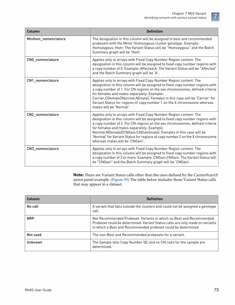
Chapter 7 MSV VariantIdentifying variants with various variant status 7
Note: There are Variant Status calls other than the ones defined by the CarrierScan1S annot.panel example. (Figure 55) The table below includes those Variant Status calls that may appear in a dataset.
MinHom_nomenclature The designation in this column will be assigned to best and recommended probesets with the Minor Homozygous cluster genotype. Example: Homozygous; Hom: The Variant Status will be "Homozygous" and the Batch Summary graph will be 'Hom'.
CN0_nomenclature Applies only to arrays with Fixed Copy Number Region content. The designation in this column will be assigned to fixed copy number regions with a copy number of 0. Example: Affected;A. The Variant Status will be "Affected" and the Batch Summary graph will be 'A'.
CN1_nomenclature Applies only to arrays with Fixed Copy Number Region content. The designation in this column will be assigned to fixed copy number regions with a copy number of 1. For CN regions on the sex chromosomes, defined criteria for females and males separately. Example: Carrier;C[female]|Normal;N[male]. Females in this case will be 'Carrier' for Variant Status for regions of copy number 1 on the X chromosome whereas males will be 'Normal'.
CN2_nomenclature Applies only to arrays with Fixed Copy Number Region content. The designation in this column will be assigned to fixed copy number regions with a copy number of 2. For CN regions on the sex chromosomes, defined criteria for females and males separately. Example: Normal;N[female]|CNGain;CNGain[male]. Females in this case will be 'Normal' for Variant Status for regions of copy number 2 on the X chromosome whereas males will be 'CNGain'.
CN3_nomenclature Applies only to arrays with Fixed Copy Number Region content. The designation in this column will be assigned to fixed copy number regions with a copy number of 3 or more. Example: CNGain;CNGain. The Variant Status will be "CNGain" and the Batch Summary graph will be 'CNGain'.
Column Definition
Column Definition
No call A variant that falls outside the clusters and could not be assigned a genotype call.
NRP Not Recommended Probeset. Variants in which no Best and Recommended Probeset could be determined. Variant Status calls are only made on variants in which a Best and Recommended probeset could be determined.
Not used The non-Best and Recommended probesets for a variant.
Unknown The Sample fails Copy Number QC and no CN calls for the sample are determined.
RHAS User Guide 73

Chapter 7 MSV VariantIdentifying variants with various variant status 7
Variant summary matrix
The Matrix graphs all the variant calls for each sample in the Sample Table.The matrix is useful for easily visualizing trends for a given variant or sample. The figure below shows several non-normal variant calls in Sample 2. This would be unexpected and may indicate a quality issue with the sample. Looking horizontally at Figure 56, several non-normal calls for a specific variant are highlighted. This may or may not be expected, but shows that the matrix is a useful tool to quickly identify trends in both samples and variants.
The filters applied to the Selected Sample Variants table are also applied to the Variant Summary Matrix graph on the right side. When the Standard filters are applied, variants called as part of the major homozygous cluster (i.e. Not Detected, Absent, or Normal) appear as a gray cell in the matrix as they are filtered out. Variants with only major homozygous calls across all samples are also filtered out.
Figure 56 Matrix graph example
RHAS User Guide 74

Chapter 7 MSV VariantIdentifying variants with various variant status 7
Figure 57 is an example of a Variant Summary Matrix table with no applied filter (left) and one with standard filters applied (right).
Cluster graph The Cluster Graph displays the ProbeSet calls for loaded samples as a set of points in the clustering space used for making the calls. A visual inspection of select Cluster Plots aids in determining Variant Status calls such as No Calls or NRP.By default, the Cluster Graph is set for auto-detecting the Graph Type (Auto). The Cluster Graph auto-selects the appropriate graph type based on the type of probeset. For bi-allele probesets (those that measure two alleles), only the Contrast view displays the ellipses that illustrate the prior and posterior knowledge of genotype cluster positions. Multi-allele probesets measure more than two alleles. Unlike bi-allele probesets, multiallele probesets are genotyped in the Log2 Signal space. For multi-allele probesets, the ellipses that illustrate the prior and posterior knowledge of genotype cluster positions are only displayed when selecting the plot type Log2 Signal. Figure 58 shows examples of a bi-allele Cluster Graph (left) and a multi-allele Cluster Graph (right).
Figure 57 Variant Summary Matrix example - No filtering applied (left) vs. Standard filtering applied (right)
RHAS User Guide 75

Chapter 7 MSV VariantIdentifying variants with various variant status 7
Cluster graph options
Use the Graph’s menu drop-down menus (Figure 59) to customize your Cluster Graph.
Prior (or MA Prior): Defines prior knowledge of SNP cluster locations. This file has the same format as a posteriors file, which is generated by the genotyping step. This means that you can “train” on a custom data set, and use the updated knowledge of cluster locations as a “seed” to possibly improve future genotyping batches.Posterior (or MA Posterior): Generated during the genotyping step. Specifies identified SNP probeset cluster locations, variance, and relative weight.Special SNPs: When the expected copy number is less than two, chromosomes Y, MT, and non-PAR X will also be assigned hemizygous and ZeroCN genotype codes.
Figure 58 Cluster Graph example - Bi-allele (left) vs. Multi-allele (right)
Figure 59 Cluster Graph option menus
RHAS User Guide 76

Chapter 7 MSV VariantReviewing variant status calls 7
Reviewing variant status calls
Use the Sample Table, Selected Sample Variant Table, Cluster Plot and SNP Summary Table to review variant status calls in your dataset.
Figure 60 shows a selected sample highlighted in the Sample Table. This sample has two Variants Status as ́ No Callʹ. Use the Cluster Graph and the Sample Table to review these two variants to assist in determining a probable Variant Status call.
1. Select a variant that has a No Call in the Selected Sample Variant Table, then click on the Cluster Graph (right).The Cluster Graph will automatically be selected to the probeset of the variant you highlighted in the Selected Sample Variant Table.
2. Initiate SNP Prior Viewing by selecting Default Priors from the Prior drop-down located at the bottom of the Cluster Graph.
3. Review the data point for the selected sample (highlighted inside a pink circle).Figure 60, shows the sample’s data is well below the Major Homozygous cluster and also is not near the clusters that would be heterozygous (yellow) or minor homozygous (red).The dotted ellipses in the cluster plot are the SNP ́ Priorsʹ. These regions are where the algorithm expects the data for the cluster might be. After running the clustering algorithm, the posteriors (solid ellipse) indicate where the algorithm finished clustering the data.
Figure 60 Sample Table and Cluster Graph
RHAS User Guide 77

Chapter 7 MSV VariantReviewing variant status calls 7
If you want to see if there are other probesets designed for this variant that were not selected by the algorithm as the Best and Recommended, do the following:
1. Click on the SNP Summary Table window tab. (Figure 61)
The current probeset are selected in the SNP Summary window.2. Sort by Affy SNP ID. For sorting instructions, see ʺSorting columnsʺ on page 36.
Sorting by Affy SNP ID groups all probesets associated with a variant. In Figure 61, the current probeset is the only one assaying the variant.Note: After selecting the SNP Summary Table, the lower pane automatically shifts to the Genotyping data for all samples for the variant. As the Cluster Graph shows in Figure 61, the signal for the datapoint is much lower than the major homozygous cluster. The Genotyping Data in the table confirms this lower signal as well. As you can see, the Allele A and Allele B signals are less than half of those with genotype calls in the major homozygous cluster. This can be due to either the result of an interfering variant (another nearby SNP that is impacting the signal of the probeset assaying this variant) or a loss in copy number in the region around the variant.Depending on the array type, you can check the copy number for the region of this variant. If we refer back the Selected Sample Variant Table, we see there is another variant in the same gene that has a status of ́ No Callʹ. Repeating the steps outlined above, shows the probeset for this second variant also has depressed signal relative to the major homozygous cluster. (Figure 62)
Figure 61 SNP Summary Table and Cluster Graph
RHAS User Guide 78

Chapter 7 MSV VariantReviewing variant status calls 7
The Selected Sample Variant Table shows that the two variants are within 35 bases of each other. The depressed signals could still be a result of an interfering variant, but that scenario is less likely. To verify this, you must check the copy number in the gene region. To do this:
1. Click on the CN Window.2. Select the sample from the Sample Table.3. In the Whole Genome Graph, search for the gene.4. Check the data types for the selected sample in the lower right pane for a loss in
copy number.
Figure 62 Example: Depressed signal relative to the major homozygous cluster
RHAS User Guide 79

Chapter 7 MSV VariantReviewing variant status calls 7
Figure 63 displays a copy number loss in the region where these two variants are located. This example explains the reason for the lower signal, as there is only one allele present.
SNP summary table columns
The SNP Summary Table provides information about the probesets and markers interrogated on the array. The standard/default SNP Summary Table columns listed below give performance and additional information for each probeset.
Figure 63
Column Definition
Probeset_ID Thermo Fisher Scientific identifier for the probeset.
Affy SNP ID Unique Thermo Fisher Scientific generated identifier for the SNP
RHAS User Guide 80

Chapter 7 MSV VariantReviewing variant status calls 7
RS ID dbSNPID
ConversionType Probeset classification
CR Call rate (CR) is the percentage of samples with a genotype call other than "No Call" for the SNP. Note: Call Rate on non-pseudoautosomal regions of chromosome X is reported only for female samples. Call Rate on chromosome Y is reported only for male samples.
MinorAlleleFrequency The allele frequency for the A allele is calculated as:
Where the Total # Calls does not include the No Calls. The B allele frequency is . The minor allele frequency is the Min(PA, PB).
H.W.p-Value Hardy Weinberg p-value is a measure of the significance of the discrepancy between the observed ratio or heterozygote calls in a population and the ratio expected if the population was in Hardy Weinberg equilibrium.
There are two statistical tests used for HWE. When AA, AB, and BB counts are all >=10, a Chi-squared test is used. When one or more of the AA, AB, and BB counts are <10, an Exact test is used. An Exact test means that the p-value is calculated exactly and not approximated from a population distribution.
Where:
Where CDF is the Cumulative Distributive Function for the chi-squared distribution. The Exact test used is the one implemented in R package "HardyWeinberg". For more information see: [2] Haldane, J., 1954. An exact test for randomness of mating. J. Genet. 52 631-635. [3] Levene, H., 1949. On a matching problem arising in genetics. Ann. Math. Stat. 20 91-94.
Column Definition
RHAS User Guide 81

Chapter 7 MSV VariantReviewing variant status calls 7
nMinorAllele The count of minor alleles, which is one for each heterozygous call, one for each minor haploid call, and two for each minor homozygous call.
Nclus The number of genotype clusters.
n_AA The number of AA calls.
n_AB The number of AB calls.
n_BB The number of BB calls.
n_NC The number of NoCall calls, including NoCall_1 (haploid).
BestProbeset BestProbeset flag is available when multiple probesets are mapped to the same SNP (affy_snp_id) by a ps2snp file. A probeset is selected based on the priority order of the conversion types. BestProbeset flag is 1 when it is the best or only probeset for a SNP. Otherwise the flag is 0.
Chr Chromosome on which the varaint was found.
Min Start position of variant.
Max End position of variant.
Column Definition
RHAS User Guide 82

Chapter 7 MSV VariantSNP metrics summary 7
SNP metrics summary
The SNP Summary Metrics window tab displays a summary snapshot of your analysis, including detailed threshold values, and tables based on your analysis, as shown in Figure 64.
Figure 64 SNP Metrics Summary - Best Practices workflow example
SNP Metrics Summary: Contains a summary of the categorization of probesets in the analysis by PS_Classification.
Marker Metrics Summary: Contains a break-down summary of the number of markers that are in BestandRecommended category, percentage, and conversion type.
RHAS User Guide 83

8 MSV SMN
Introduction
The Survival of Motor Neuron analysis algorithm is designed to identify samples that potentially have < 2 copies of SMN1. SMN analysis assesses batches of samples and generates a single status call for each sample. SMN analysis also flags samples that have non-major homozygous calls for a user-defined set of SMN variants. Note: Follow up on all non-normal sample status calls is recommended.
Features
• Novel algorithms to test for SMN1 based copy number status.• Graphical depiction of SMN copy number.• Flexibility to add genotype information of user-defined SMN SNPs into the
results.
SMN window
1. Click on the SMN menu link (far left). Note: This link is only visible on CHP files after a SMN analysis has been successfully run.The main SMN Result window appears. (Figure 65)The data displayed in the SMN window is by analysis batch only. You may have multiple analysis batches loaded into the MSV, but the display will group them by analysis batch. You can toggle from batch to batch using the Current Batch drop-down which lists all your loaded analysis batches.
RHAS User Guide 84

Chapter 8 MSV SMNUsing the table and plots 8
Using the table and plots
See Chapter 4, ʺMSV setup and featuresʺ on page 29 for common table and graph functions.
1. Single-click on a sample listed on the table. The sample is now reflected in the Copy Number Batch Plot graph and Sample SMN Copy Number Plot (lower left), as shown in Figure 66.Alternatively, single-click on any Copy Number Batch Plot sample to view it’s placement and properties in the table and its subsets, as shown in Figure 67.
Figure 65 Main SMN Result window
Sample Table
Sample CN Plot
SMN CN Scatter Plot
RHAS User Guide 85

Chapter 8 MSV SMNUsing the table and plots 8
Figure 66 Highlighted sample shown in plots
RHAS User Guide 86

Chapter 8 MSV SMNUsing the table and plots 8
Sample SMN copy number plot
Note: The (lower left) Sample SMN Copy Number plot is for display purposes only. Use this plot to view a highlighted sample’s analyzed subset result. The example shown in Figure 67 depicts the overall SMN1 copy number state for the Sample and how it compares to individual assessment at Exon7 and Exon8.
= Normal = Carrier
Figure 67 Example: Single sample SMN copy number plot
Sample
Sample subset
Sample subset
RHAS User Guide 87

Chapter 8 MSV SMNAdding SMN SNPs to the results 8
Adding SMN SNPs to the results
SMN SNPs can be added to the results by adding the following information to the tab delimited snplist.txt file (Figure 68). This file can be found in the array library file package. Note: Before SNPs can be included in the SMN results, the SNP probeset(s) must be included in the step2 list for genotyping.
Figure 68 Example snplist.txt file for the CarrierScan1S array
(A) probeset_id (Required) The probeset for the SMN SNP variant to be added to the output.
(B) affy_snp_id (Required) The affy_snp_id associated with the probeset ID.
(C) ref_code (Required) The call code (generally A or B for bialleles) associated with the alternate allele.
(D) alt_code (Required) The call code (generally A or B for bialleles) associated with the alternate allele.
(E) ref_allele (Required) The nucleotide assigned to the reference allele.
(F) alt_allele (Required) The nucleotide assigned to the alternate allele.
(G) variant (Required) Variant name.
(H) comments (Optional) Use this text field to enter comments. Note: Comments are not used in the analysis.
RHAS User Guide 88

A Definitions
Sample table
Columns for selection vary, as they are dependent upon array type(s) loaded in MSV.
Table 1 Sample table
Column Definition
# Gain (Mosaic) Seg (# Count)
Number of mosaic gain segments in the sample (based on current filter settings)
# Gain Seg (# Count) Number of gain segments in the sample (based on current filter settings)
# Gain/Loss (Mosaic) Seg (# Count) Total number of both mosaic gain and mosaic loss segments in the sample (based on current filter settings)
# Gain/Loss Seg (# Count)
Total number of both gain and loss segments in the sample (based on current filter settings)
# LOH seg (# Count) Number of LOH segments in the sample (based on current filter settings)
# Loss (Mosaic) Seg(# Count)
Number of mosaic loss segments in the sample (based on current filter settings)
# Loss Seg (# Count) Number of loss segments in the sample (based on current filter settings)
# Somatic Mutation(# Count)
Number of Detected Somatic Mutations (OncoScan only)
# Variants (Table-WGV) (# Count) Number of Variants Detected in the Variants tab in the Copy Number window. Number of variants reported in this column is dependent upon filters applied.
# Variants (Table) (# Count)
Number of Variants Detected in the Variants tab in the Variant window. Number of variants reported in this column is dependent upon filters applied.
Algorithm Name Name of the algorithm used in processing the array.
Algorithm Version Version of the algorithm used in processing the array.
All Probeset RLE Mean The mean absolute relative log expression (RLE) – This metric is generated by taking the probe set summary for a given array and calculating the difference in log base 2 from the median value of that probe set over all the arrays. The mean is then computed from the absolute RLE for all the probe sets for a given CEL file.
Antigenomic Ratio Ratio of median intensity antigenomic control probes/median intensity all copy numberprobes.
RHAS User Guide 89

Appendix A DefinitionsSample table A
Array Annotation File Name of the Annotation file used to create the xxCHP file.
Array Package Library file package used for RHAS analysis.
Autosome LOH The proportion of LOH on chromosome 1 to 22.
Barcode Cartridge or Plate Barcode depending on array type
Batch Female Count Number of females in the analysis run
Batch Male Count Number of males in the analysis run
Batch Plate Sample Count Number of females per plate in the analysis run
Batch Sample Count Number of males per plate in the analysis run
CEL File Name of the CEL file from which the CHP file was generated
CEL File Path Location of the CEL at the time of analysis
Cel Pair Check Inspects each pair of intensity (*.cel) files to determine whether the files have been properlypaired and assigned to the correct channel.
Cel Pair Check Call Rate AT Call Rate for SNPs used in the Cel Pair Check for the AT channel array
Cel Pair Check Call Rate GC Call Rate for SNPs used in the Cel Pair Check for the GC channel array
Cel Pair Check Concordance Percentage of SNPs that match between the AT and GC arrays.
CHP File Date Date the xxCHP file was created
CHPCAR Yes/No as to whether a chpcar file exists for the sample
CN Control Chosen Yes/No as to whether the sample was selected as a CN control for plate correction
CN Control Used Yes/No as to whether the sample was used (based on passing QC) as a CN control for plate correction
CN Seg Overlaps CytoRegion Yes/No as to whether the sample has a copy number segment that overlaps an annotation in a loaded CytoRegion file
CN Tuned Using Controls Yes/No as to whether the copy number for the sample was tuned using the selected CN Controls
Custom Log 2 Ratio Adj User defined median Log 2 ratio entered during recentering
Frequency Heterozygous Call Percentage heterozygous call for the sample
Frequency Homozygous Call Percentage homozygous call for the sample
DQC Log Diff QC (Geno QC) A cross channel QC metric, defined as mean(log(AT_SBR))/std(log(AT_SBR))+mean(log(GC_SBR))/std(log(GC_SBR)), where signal and background are calculated for control non-polymorphic probes after intensity normalization.
Signal Contrast A Signal Mean (Geno QC)
Average of control A probe raw intensities in the AT channel.
Table 1 Sample table
Column Definition
RHAS User Guide 90

Appendix A DefinitionsSample table A
Signal Contrast AT B (Geno QC) AT channel background, which is the average signal of the GC control probes in AT channel.
Signal Contrast AT B IQR (Geno QC) AT channel interquartile range (middle 50%) of background intensities, measured using GC control probes.
Signal Contrast AT FLD (Geno QC) Fisher's Linear Discriminant between signal and background in the AT channel, defined as [median_of_AT_probe_intensities –median_of_GC_probe_intensities]2 / [0.5*(AT_S_IQR2 + AT_B_IQR2)].
Signal Contrast AT S (Geno QC) AT channel signal, which is the average signal of the AT control probes in AT channel.
Signal Contrast AT S IQR (Geno QC) AT channel interquartile range (middle 50%) of signal intensities, measured using AT control probes.
Signal Contrast AT SBR (Geno QC) AT channel signal to background ratio, defined as AT_S/AT_B.
Signal Contrast C Signal Mean (Geno QC)
Average of control C probe raw intensities in the GC channel.
Signal Contrast G Signal Mean (Geno QC) Average of control G probe raw intensities in the GC channel.
Signal Contrast GC B IQR (Geno QC) GC channel interquartile range (middle 50%) of background intensities, measured using AT control probes.
Signal Contrast GC B (Geno QC) GC channel background, which is the average signal of the AT control probes in GC channel.
Signal Contrast GC FLD (Geno QC) Fisher's Linear Discriminant between signal and background in the GC channel, defined as [median_of_GC_probe_intensities –median_of_AT_probe_intensities]2 / [0.5*(GC_S_IQR2 + GC_B_IQR2)].
Signal Contrast GC S (Geno QC) GC channel signal, which is the average signal of the GC control probes in GC channel.
Signal Contrast GC S IQR (Geno QC) GC channel interquartile range (middle 50%) of signal intensities, measured using GC control probes.
Signal Contrast GC SBR (Geno QC) GC channel signal to background ratio, defined as GC_S/GC_B.
Signal Contrast T Signal Mean (Geno QC) Average of control T probe raw intensities in the AT channel.
Genome LOH The proportion of LOH across the whole genome.
Genome Version Genome Build (i.e. hg38)
Allele Deviation Mean (Genotyping) Average of the absolute difference between the log2 allele signal estimate and its median across all arrays (measured at the Sample QC step).
Allele Deviation Stdev (Genotyping) Standard deviation of the absolute difference between the log2 allele signal estimate and its median across all arrays.
Allele Mad Residuals Mean (Genotyping) Average of the median absolute deviation (MAD) between observed probe intensities and probe intensities fitted by the model.
Allele Mad Residuals Stdev (Genotyping) Standard deviation of the median absolute deviation (MAD) between observed probe intensities and probe intensities fitted by the model.
Table 1 Sample table
Column Definition
RHAS User Guide 91

Appendix A DefinitionsSample table A
Allele Summarization Mean (Genotyping) Average of the allele signal estimates (log2 scale).
Allele Summarization Stdev (Genotyping) Standard deviation of the allele signal estimates (log2 scale).
Application (Reproseq) Name of Application from the ReproSeq assay
Call Rate (Genotyping) Percentage of autosomal SNPs with a call other than NoCall. 'SpecialSNP' probesets are excluded, as they are mostly non-autosomal.
ChrMA (Reproseq) Ratio of Mitochondria:Autosome
Cluster Distance Mean (Genotyping) Average distance to the cluster center for the called genotype.
Cluster Distance Stdev (Genotyping) Standard deviation of the distance to the cluster center for the called genotype.
CN Probe ChrXY Ratio Gender MeanX (Genotyping)
Average probe intensity (raw, untransformed) of X chromosome nonpolymorphic probes.
CN Probe ChrXY Ratio Gender MeanY (Genotyping)
Average probe intensity (raw, untransformed) of Y chromosome nonpolymorphic probes.
Het Rate (Genotyping) Percentage of SNPs called AB (i.e. the heterozygosity) for autosomal SNPs.
Hom Rate (Genotyping) Percentage of SNPs called AA or BB (i.e. the homozygosity) for autosomal SNPs.
Max Num Alleles (Genotyping) The maximum number of alleles for a given variant in the sample.
Total Call Rate (Genotyping) Call rate at the default or user-specified threshold for all SNPs.
Total Het Rate (Genotyping) Percentage of SNPs called AB (i.e., the heterozygosity) for all SNPs.
Total Hom Rate (Genotyping) Percentage of SNPs called AA or BB (i.e. the homozygosity) for all SNPs.
DQC Bound (Genotyping QC) Yes/No. Did the sample meet the threshold for this metric
GT PlateQC Avg CR Bound (Genotyping QC)
Yes/No. Did the sample meet the threshold for this metric
GT PlateQC Passing % Bound (Genotyping QC)
Yes/No. Did the sample meet the threshold for this metric
QC Allele Deviation Mean (Genotyping QC)
Average of the absolute difference between the log2 allele signal estimate and its median across all arrays (measured at the Sample QC step).
QC Allele Deviation Stdev (Genotyping QC)
Standard deviation of the absolute difference between the log2 allele signal estimate and its median across all arrays (measured at the Sample QC step).
QC Mad Residuals Mean (Genotyping QC) Average of the median absolute deviation (MAD) between observed probe intensities and probe intensities fitted by the model (measured at the Sample QC step).
QC Mad Residuals Stdev (Genotyping QC) Standard deviation of the median absolute deviation (MAD) between observed probe intensities and probe intensities fitted by the model (measured at the Sample QC step).
Table 1 Sample table
Column Definition
RHAS User Guide 92

Appendix A DefinitionsSample table A
QC Allele Summarization Mean (Genotyping QC)
Average of the allele signal estimates (log2 scale) (measured at the Sample QC step).
QC Allele Summarization Stdev (Genotyping QC)
Standard deviation of the allele signal estimates (log2 scale) (measured at the Sample QC step).
QC Call Rate Bound (Genotyping QC) Yes/No. Did the sample meet the threshold for this metric
QC Cluster Distance Mean (Genotyping QC)
Average distance to the cluster center for the called genotype (measured at the Sample QC step).
QC Cluster Distance Stdev (Genotyping QC)
Standard deviation of the distance to the cluster center for the called genotype (measured at the Sample QC step).
QC CN Probe ChrXY Ratio Gender MeanX (Genotyping QC)
Average probe intensity (raw, untransformed) of X chromosome nonpolymorphic probes (measured at the Sample QC step).
QC CN Probe ChrXY Ratio Gender MeanY (Genotyping QC)
Average probe intensity (raw, untransformed) of Y chromosome nonpolymorphic probe (measured at the Sample QC step).
QC CN Probe ChrXY Ratio Gender Ratio (Genotyping QC)
Gender ratio Y/X = cn-probe-chrXY-ratio_gender_meanY / cn-probe-chrXYratio_gender_meanX (measured at the Sample QC step).
QC Het Rate (Genotyping QC) Percentage of SNPs called AB (i.e. the heterozygosity) for autosomal SNPs (measured at the Sample QC step).
QC Hom Rate (Genotyping QC) Percentage of SNPs called AA or BB (i.e. the heterozygosity) for autosomal SNPs (measured at the Sample QC step).
QC Total Call Rate (Genotyping QC) Call rate at the default or user-specified threshold for all SNPs (measured at the Sample QC step).
QC Total Het Rate (Genotyping QC) Percentage of SNPs called AB (i.e., the heterozygosity) for all SNPs (measured at the Sample QC step).
QC Total Hom Rate (Genotyping QC) Percentage of SNPs called AA or BB (i.e. the homozygosity) for autosomal SNPs (measured at the Sample QC step).
Log 2 Ratio Adjustment (Total Custom) TuScan Log 2 Ratio Adjustment + Custom Log 2 Ratio Adjustment after manual recentering
LOH Seg Overlaps CytoRegion Yes/No as to whether the sample has an LOH segment that overlaps an annotation in a loaded CytoRegion file
Low Diploid Flag An essential part of the algorithm is the identification of "normal diploid" markers in the cancer samples. This is particularly important in highly aberrated samples. The normal diploid markers are used to calibrate the signals so that "normal diploid markers" result in a log2 ratio of 0 (e.g. copy number 2). The algorithm might later determine that the "normal diploid" markers identified really correspond to (for example) CN=4. In this case the log2 ratio gets readjusted and TuScan ploidy will report 4. Occasionally (in about 2% of samples) the algorithm cannot identify a sufficient number of "normal diploid" markers and no "normal diploid calibration occurs. This event triggers "low diploid flag" = YES. In this case the user needs to carefully examine the log2 ratios and verify if re-centering is necessary.
Manufacturer Thermo Fisher Scientific
Table 1 Sample table
Column Definition
RHAS User Guide 93

Appendix A DefinitionsSample table A
MAPD Bound Yes/No. Did the sample meet the threshold for this metric
MAPDc Bound Yes/No. Did the sample meet the threshold for this metric
ndSNPQC QC metric for SNP probes that is derived from polymorphic SNP probes in normal diploid regions.
ndwavinessSD Measure of variation of probes in normal diploid regions that are insensitive to short-range variation and focus on long-range variation.
Number nd Number of probes called normal diploid by the algorithm.
Number of Controls for CN Tuning A count of control samples used to adjust the CN signals for the given sample. This value will be the same for all samples on the same plate.
Option Reference File Copy number Ref Model File
Option Reference File Name Location of the copy number Ref Model File
Percent nd Percentage of probes called normal diploid by the algorithm
Plate Barcode Barcode of the array plate
Reference Reference Model file used in the single sample analysis.
RHAS CHP File Version CHP file version created by RHAS analysis
CN Control Chosen (SMN) Yes/No as to whether the sample was selected as a CN control for plate correction for the SMN pipeline
CN Control Used (SMN) Yes/No as to whether the sample was used (based on passing QC) as a CN control for plate correction for the SMN pipeline
MAPD Bound (SMN) Yes/No. Did the sample meet the threshold for this metric.
Number of Controls for CN Tuning (SMN) Number of control samples used when tuning copy number for the SMN pipeline
SMN Status (SMN) Status call for the sample based on SMN1 copy number
SMN1 CN (SMN) Copy number for SMN1.
SMN1 Exon 7 (SMN) Copy number for Exon 7 of SMN1.
SMN1 Exon 8 (SMN) Copy number for Exon 8 of SMN1.
SMN1 [variant] Genotype call for SMN variant(s) as defined in the SMN.SNP.list
SMN1 [variant] Call Reference and Alternate Allele call for SMN variant(s) as defined in the SMN.SNP.list
SMN2 CN Copy number for SMN2.
Waviness SD Bound (SMN) Yes/No. Did the sample meet the threshold for this metric
SNP QC Type ND or non-ND
Table 1 Sample table
Column Definition
RHAS User Guide 94

Appendix A DefinitionsSample table A
SNR This metric is the Signal/Noise Ratio of markers in both the AT and GC channels. The Signal is the 65th percentile of the measurements used for copy number analysis, minus the median of the antigenomic features. The Noise is the standard deviation of the weakest 15% of measurements used for copy number analysis. A low value indicates poor data quality.
SNR AT This metric is the Signal/Noise Ratio of markers in the AT channel. The Signal is the 65th percentile of the measurements used for copy number analysis, minus the median of the antigenomic features. The Noise is the standard deviation of the weakest 15% of measurements used for copy number analysis. A low value indicates poor data quality from the AT CEL file.
SNR GC This metric is the Signal/Noise Ratio of markers in the GC channel. The Signal is the 65th percentile of the measurements used for copy number analysis, minus the median of the antigenomic features. The Noise is the standard deviation of the weakest 15% of measurements used for copy number analysis. A low value indicates poor data quality from the GC CEL file.
SOM Annotation File The Somatic Mutation annotation database used
SOM CEL Pairs File Workflow file showing matched CEL pairs
SOM Count High Number of Somatic Mutation detected with ‘High Confidence’
SOM Count Low Number of Somatic Mutation detected with ‘Low Confidence’
SOM Panel/Somatic Mutation File Version of Somatic Mutation Panel
SOM Reference File Reference Model file used in Somatic Mutation detection
SOM Thresholds File Thresholds file used in determining Somatic Mutation detected calls
TuScan %AC If % AC = 100%, we return "homogeneous" because it could be 100% normal or 100% tumor. If % AC =NA, the percent aberrant cells could not be determined and TuScan returns non-integer CN calls. This metric is an algorithmically determined estimate of the % of aberrant cells in the sample.
TuScan %ACDC Indicates whether the algorithm was able to compute the % Aberr. Cells and measure the Copy Number in the tumor cells only. “ACDC= No” means Copy Number was calculated as an average CN across all cells, “ACDC=Yes” means that Copy Number was calculated only for the tumor cells.
TuScan Log 2 Adjustment Log 2 ratio determined from TuScan algorithm needed to "center" the diploid region of the sample (around Log 2 = 0).
TuScan Median Ploidy Ploidy state for the whole sample including both tumor and normal fractions.
TuScan Ploidy The most likely ploidy state of the tumor before additional aberrations occurred. TuScan Ploidy is assigned the median CN state of all markers, provided that %AC could be determined and integer copy numbers are returned. If %AC cannot be determined, NA (Not Available) is reported for both ploidy and %AC.
Table 1 Sample table
Column Definition
RHAS User Guide 95

Appendix A DefinitionsSample table A
Associated Genes (Variants) Name of heritable genetic sequence that encodes proteins.
Associated Phenotypes (Variants) Displays the Phenotype that is associated with the variant.
Panel File (Variants) Name of the annot.panel file used in the Variant portion of the analysis.
Variants Detected (Variants) Number of Variants with a non-normal call
Variants Tested (Variants) Number of variants tested in the analysis (number of variants included in the step2 list)
Variants to Review (Variants) Number of Variants that need to be manually reviewed such as No Calls or NRP.
Waviness SD Bound Yes/No. Did the sample meet the threshold for this metric
Waviness SDc Bound Yes/No. Did the sample meet the threshold for this metric
Well Position Location of samples on the array plate
Workflow Config Name Name of the configuration settings used in the analysis (i,e Default)
Workflow Type of Workflow using in analysis (i.e. Best Pracitces)
Workflow (ReproSeq) Name of the workflow run in Ion Reporter.
Table 1 Sample table
Column Definition
RHAS User Guide 96

Appendix A DefinitionsCopy number window A
Copy number window
Segment table column options
Columns shown in BOLD are default/standard view selections.
Table 2 Segment columns
Column Name Definition
File File the segment was detected in.
Type Type of segment. Gain, Loss, Gain (Mosaic) or Loss (Mosaic)
State Copy Number State
Chr Chromosome on which the segment was found.
Min Start position of segment.
Max End position of segment.
Size (kpb) Size of segment.
Marker Count Number of markers in the segment.
Within CytoRegion Names of the CytoRegions with which the segment shares coordinates.
Call This field is read-only in the MSV and is populated using Chromosome Analysis Suite (ChAS). It is a user-editable field populated by a user-configurable drop list of Calls in ChAS. If Calls have not been assigned to a segment in ChAS, this field will be blank. See the ChAS User Guide for details.
Call Approval This field is read-only in the MSV and is populated using Chromosome Analysis Suite (ChAS). This column can be used as a bookmark for segments that have been reviewed. See the ChAS User Guide for details.
Curation By This is a read-only field in the MSV. The user who last edited or annotated the segment in ChAS.
Curation Time This is a read-only field in the MSV. The time and date when the Curation field was last edited.
Inheritance This field is read-only in the MSV and is populated using Chromosome Analysis Suite (ChAS). It is a user-editable field populated by a user-configurable drop list for Inheritance in ChAS. If Inheritance has not been assigned to a segment in ChAS, this field will be blank. See the ChAS User Guide for details.
Mean Marker Distance Length of the segment in base pairs divided by the number of markers in the segment
Segment Interpretation This field is read-only in the MSV and is populated using Chromosome Analysis Suite (ChAS). It is a user-editable field populated by text or from a user-defined list of short phrases. If this field have not been populated for a segment in ChAS, this field will be blank. See the ChAS User Guide for details.
RHAS User Guide 97

Appendix A DefinitionsCopy number window A
Copy number segments on the X and Y chromosomes
The expected copy number state on the X chromosome in normal males is not constantover its entire length. This is due to the structure of the sex chromosomes, and the factthat they share extensive homology with each other only in the Pseudo AutosomalRegions (PARs) that they each have at either end. PAR1 is at the top of the p-arm andPAR2 at the bottom of the q-arm.
Markers occurring in the PAR regions are mapped exclusively to the X Chromosome.Therefore, in normal males the PAR regions of the X are expected to be CN=2 (probeson the X and Y contribute to the signal), while the rest of the Chr X is expected CN=1for normal males. As a result, we treat the two X PARs in males as independent units(CN=2 expected) from the rest of the X chromosome (CN=1 in males) when generatingCopy Number Segments.
Aberrant segments that cross PAR/non-PAR boundaries may be normalized into onesegment if they have equivalent type (Gain or Loss) and CN State. During thisnormalization process, RHAS will not combine an aberrant (Gain or Loss) segmentwith a normal segment across PAR/non-PAR boundaries, even if they have the sameCN State. If smoothing is subsequently applied, aberrant segments with different copynumber state may be combined. If joining is subsequently applied, aberrant segmentsseparated by a non-aberrant segment may be combined.Because only Y-specific probes are mapped to the Y chromosome, the expected state ofthe entire Y chromosome is 1 for males and is 0 for females.
Mosaic CN segments on the X chromosome
The expected copy number state on the X chromosome in normal males is not constantover its entire length. This is due to the structure of the sex chromosomes and the factthat they share extensive homology with each other only in the Pseudo AutosomalRegions (PARs) that they each have at either end. PAR1 is at the top of the p-arm andPAR2 at the bottom of the q-arm.
Markers occurring in the PAR regions are mapped exclusively to the X Chromosome.Therefore, in normal males the PAR regions of the X are expected to be CN=2 (probeson the X and Y contribute to the signal), while the rest of the Chr X is expected CN=1for normal males.
Mosaic Segments whose boundaries start and end entirely in one of the PAR regionswill use CN=2 as normal to determine the type (GainMosaic or LossMosaic) of Mosaicsegment to draw.
Because the Mosaicism algorithm can generate segments which cross the PARboundaries, Mosaic Segments that touch the non-PAR region of the X chromosome usethe gender call of the sample to determine the Type of Mosaic segment to draw.Because only Y-specific probes are mapped to the Y chromosome, the expected state ofthe entire Y chromosome is 1 for males and is 0 for females.
RHAS User Guide 98

Appendix A DefinitionsCopy number window A
LOH table column options
Columns shown in BOLD are default/standard view selections.
Table 3 LOH columns
Column Name Definition
File File the segment was detected in.
Type Type of segment. Gain, Loss, Gain (Mosaic) or Loss (Mosaic)
State Copy Number State
Chr Chromosome on which the segment was found.
Min Start position of segment.
Max End position of segment.
Size (kpb) Size of segment.
Marker Count Number of markers in the segment.
Within CytoRegion Names of the CytoRegions with which the segment shares coordinates.
Call This field is read-only in the MSV and is populated using Chromosome Analysis Suite (ChAS). It is a user-editable field populated by a user-configurable drop list of Calls in ChAS. If Calls have not been assigned to a segment in ChAS, this field will be blank. See the ChAS User Guide for details.
Call Approval This field is read-only in the MSV and is populated using Chromosome Analysis Suite (ChAS). This column can be used as a bookmark for segments that have been reviewed. See the ChAS User Guide for details.
Curation By This is a read-only field in the MSV. The user who last edited or annotated the segment in ChAS.
Curation Time This is a read-only field in the MSV. The time and date when the Curation field was last edited.
Inheritance This field is read-only in the MSV and is populated using Chromosome Analysis Suite (ChAS). It is a user-editable field populated by a user-configurable drop list for Inheritance in ChAS. If Inheritance has not been assigned to a segment in ChAS, this field will be blank. See the ChAS User Guide for details.
Mean Marker Distance Length of the segment in base pairs divided by the number of markers in the segment
Segment Interpretation This field is read-only in the MSV and is populated using Chromosome Analysis Suite (ChAS). It is a user-editable field populated by text or from a user-defined list of short phrases. If this field have not been populated for a segment in ChAS, this field will be blank. See the ChAS User Guide for details.
Overlap% (name of CytoRegion file) Provides the percentage overlap of the segment when a CytoRegion file(s) is assigned.
RHAS User Guide 99

Appendix A DefinitionsCopy number window A
Somatic mutation table column options
Columns shown in BOLD are default/standard view selections.
Table 4 Somatic Mutation columns
Column Name Definition
File File the segment was detected in.
Type Type of segment. Gain, Loss, Gain (Mosaic) or Loss (Mosaic)
State Copy Number State
Chr Chromosome on which the segment was found.
Min Start position of segment.
Max End position of segment.
Common Name Common name of the somatic mutation
SomMut Score Measures somatic mutation probeset response. The stronger the response, the more likely it is that the somatic mutation is present. The MutScore calculation depends on the algorithm version. The newer MutScore calculation also corrects for sample-specific effects, and thereby reduces false positive calls, which were sample specific.
For algorithm versions 1.0 - 1.2 (ChAS 3.0 and earlier, OncoScan Console 1.2 and earlier): MutScore.old = (measured quantile normalized signal - median signal for this marker in the reference model file) / (95th percentile signal for this marker in the reference model file - median signal for this marker in the reference model file).
For algorithm versions 1.3 and newer (ChAS 3.1 and newer, releases of OncoScan Console after 1.2): MutScore.new = (MutScore.old - median MutScore.old for this sample) / standard deviation of MutScore.old for this sample (where standard deviation is calculated for all but the num-outstd strongest MutScore.old for this sample, median is calculated for all but the num-out-med strongest MutScore.old for this sample, and the used median is the maximum of zero and the measured median).
COSMIC ID The identifier of the mutation as listed in the COSMIC database, which is a catalogue of somatic mutations in cancer. More information on these mutations can be found at: http://cancer.sanger.ac.uk
Accession number RefSeq Gene accession number.
Channel CEL file from which the signal is measured. "A" is the AT CEL, "C" is the GC CEL.
Event Describes if the probeset is a point mutation, deletion, insertion or sequence variant.
Event Type Describes if the event is missense, frame-shift, in-frame insertion or deletion.
Fwd 5’ flank Sequence flanking the mutation at the 5' end.
Fwd 3’ flank Sequence flanking the mutation at the 3' end.
RHAS User Guide 100

Appendix A DefinitionsCopy number window A
Genes RefSeq gene that shares coordinates with the somatic mutation.
High Threshold High confidence MutScore threshold. Measurements equal to or greater than this threshold are called “High confidence,” describing the likelihood that the mutation is present.
Low Threshold Lower confidence MutScore threshold. Measurements with a MutScore below this value are called “Undetected”. Measurements equal to or greater than this threshold but less than the High Threshold are called “Lower confidence,” describing the likelihood that the mutation is present.
Mutation (nt) Wild type > mutant nucleotide change on the coding strand.
Mutation (aa) Wild type > mutant amino acid change on the coding strand.
Mutation Syntax (aa) Encoding of which nucleotide was changed and its location in the CDS.
Mutation Syntax (cds) Encoding of which amino acid was changed and the location of the codon.
Probeset Type Probeset Type is Somatic Mutation (SOM).
Probe set Name Thermo Fisher Scientific identifier for the probeset.
QN Signal The quantile normalized signal for the mutation.
Size (bp) The size of the Somatic mutation in base pairs.
Source DB Cosmic database version.
Strand Coding strand of the associated gene (Forward or Reverse).
Tag ID Thermo Fisher Scientific identifier for the tag sequence.
Table 4 Somatic Mutation columns
Column Name Definition
RHAS User Guide 101

Appendix A DefinitionsCopy number window A
Variant table column options
Columns shown in BOLD are default/standard view selections.Note: These columns are available in the Variant tables (in both the Copy Number and Variant windows).
Table 5 Variant columns
Column Name Definition
File File the segment was detected in.
Probeset ID Thermo Fisher Scientific identifier for the probeset.
Affy SNP ID Unique Thermo Fisher Scientific generated identifier for the SNP.
RS ID dbSNP ID
Gene Name of heritable genetic sequence that encodes proteins.
c.name Common name of the variant.
Analysis Call Genotype call code for the SNP.
Variant Status Variant annotation derived from ClinVar.
Variant Status Alt Allele Annotation Severity status for the variant mapped to Alt Allele.
Recommended Probeset A quality control metric determined by SNP Polisher algorithm that chooses the best probesets querying a SNP.
Marker Type The type of marker (Indel, SNP, CN).
Chr Chromosome on which the variant was found.
Min Start position of variant.
Max End position of variant.
Alt Allele The call for the first alternate allele associated with a non-normal phenotype.
Alt Code The Call Code (A,B,C,D,...) of the Alternate Allele.
Alternate names Displays the alternative names for the variant.
Associated Phenotypes Displays the Phenotype that is associated with the variant.
Confidence The number of probesets that agree with determined sample status for that variant.
Description Detailed information about the Phenotype.
Failure Mode Provides the reason when a call isn't made for a variant. Example: The variant was a No Call for the sample or NRP indicating No Recommended Probesets were identified to make a call.
g.name Displays the genomic coordinates for the variant.
Gene:c.name Concatenation of the Gene and c.name fields.
Het_nomenclature Defined in the annot.panel file. Provides the name that will be used for heterozygous genotype calls (example, Heterozygous or Carrier).
RHAS User Guide 102

Appendix A DefinitionsCopy number window A
Inheritence Pattern Method of Inheritance (Example: AR (Autosomal Recessive), XLR (X-linked Recessive).
Majhom nomenclature Defined in the annot.panel file. Provides the name that will be used for genotype calls in the major homozygous cluster (example, Normal or Not Detected).
Minhom nomenclature Defined in the annot.panel file. Provides the name that will be used genotype calls in the major homozygous cluster (example, Homozygous or Affected).
p.name Displays the change in protein translation for the variant.
Ref Allele The call for the reference allele associated with a normal phenotype.
Ref Code The Call Code (A,B,C) of the Reference Allele.
Severity Severity and impact rating of phenotypes. A = Profound, B = Severe, U = Unclassified, based on systematic classifications. For more information, go to: https://www.ncbi.nlm.nih.gov/pubmed/25494330
Size (bp) Size in bp of the variant.
Transcript RefSeq transcript ID associated with the c.name.
Variant Status Annotation Similar information to the Variant Status Alt Allele column. Severity status for the variant mapped to Alt Allele. However, this column only provides the status when a non major homozygous cluster call is made, all other variants that are called as the Major Homozygous cluster or No Call/NRP are given an NA.
Variation ID ClinVar ID
CN0_nomenclature Defined in the annot.panel file. Provides the name that will be used for Fixed Region CN calls of copy number 0 (example, CN0 or Loss).
CN1_nomenclature Defined in the annot.panel file. Provides the name that will be used for Fixed Region CN calls of copy number 1 (example, CN1 or Loss or Normal if on the X chromosome in males).
CN2_nomenclature Defined in the annot.panel file. Provides the name that will be used for Fixed Region CN calls of copy number 2 (example, CN2 or Gain if on the X chromosome in males).
CN3_nomenclature Defined in the annot.panel file. Provides the name that will be used for Fixed Region CN calls of copy number 3 (example, CN3 or Gain).
Table 5 Variant columns
Column Name Definition
RHAS User Guide 103

Appendix A DefinitionsSNP Summary table column options A
SNP Summary table column options
Use the table of definitions below to help select your SNP Summary table columns.Most SNP Summary table metrics are calculated by gender depending on what the chromosomes are. What is displayed is restricted to the gender in the gender_metrics column. Refer to the gender_metrics definition for more information. A few metrics are calculated only for multi-allele probesets. Most metrics are calculated only for biallele probesets.Note: Some columns may not be available for selection, as they are based on the annot.db file in the library package. Some columns depend on the presence of the information in the annot.db.
Table 6 SNP Summary columns
Column Name Definition
H.W chisquared.statistic H.W.chisquared-statistic is NA if the HW p-value is calculated using the exact test, and it's the chi-squared test statistic value if the chi-squared test was used. Refer to H.W.p-Value definition (above) for more information.
minGenotypeFreqPval If the ConversionType is 'UnexpectedGenotypeFreq' (unexpectedly-high genotype frequency) then minGenotypeFreqPval is smaller than the SNP QC parameter genotype-p-value-cutoff. The metric minGenotypeFreqPval is available for supported arrays if a genotype frequency file is supplied for SNP QC, and if the genotyped sample batch size is at least as large as the SNP QC parameter ‘min-genotype-freq-samples’.
minGenotypeFreqCluster The genotype cluster for which minGenotypeFreqPval is reported.
FLD Fisher's Linear Discriminant (FLD) is a measure of the cluster quality of a probeset. High-quality probeset clusters have well-separated centers, and the clusters are narrow. FLD is measured from the SNP posteriors produced during genotyping. FLD is undefined if either the heterozygous or one of the homozygous clusters is empty.
HomFLD HomFLD is a version of FLD computed for the homozygous genotype clusters. HomFLD is undefined for probesets without two homozygous clusters.
HetSO Heterozygous Strength Offset measures how far the heterozygous cluster center sits above the homozygous cluster centers in the Size dimension (Y position). Low HetSO values are produced either by misclustering events or by the inclusion of samples that contain variations from the reference genome. Most well-clustered diploid SNPs have positive HetSO values.
HomRO Homozygote Ratio Offset is the distance to zero in the Contrast dimension (X position) from the center of the homozygous cluster that is closest to zero. If there is only one homozygous cluster, HomRO is the distance from that cluster center to zero on the Contrast dimension.
n_CN0 The number of ZeroCN calls (zero copy number).
hemizygous Hemizygous flag is 1 if the probeset measures chromsome Y or mitochondrial DNA, indicating that diploid genotypes are not possible. Otherwise the flag is 0.
HomHet HomHet flag is 1 if, when two diploid genotype clusters are present, one cluster is homozygous and the other is heterozygous. Otherwise the flag is 0.
RHAS User Guide 104

Appendix A DefinitionsSNP Summary table column options A
gender_metrics Not all probeset metrics are reported using all samples. Number of clusters (Nclus) is calculated on all samples. See the Call Rate (CR) definition for samples used. The remaining metrics are displayed using the sample set described in gender_metrics. If gender_metrics is 'all', all samples are used. The metrics are calculated by gender depending on the chromosomes. What is displayed is restricted to the gender in the gender_metrics column. For chromosomes MT and CP: all genders, no splitting by gender. Chromosome X: all metrics on females, some metrics on males. Chromosome Y: all metrics on males, a small number of metrics on females. For avian species, chromosome Z: all metrics on males, some metrics on females and chromosome W: all metrics on females, a small number of metrics on males.
MinMean_cp_2 For multiallelic probesets, the minimum mean log2 allele signal for samples that appear to have at least two copies of that allele. If this value is not between the thresholds for the SNP QC parameters 'min-mean-cp2-cutoff' and 'max-mean-cp2-cutoff', then the probeset fails this QC test.
minSigBgndDiffHom For multiallelic probesets, minimum difference between mean log2 signal and background for the homozygous genotype clusters. If this value is less than the threshold for the appropriate SNP QC parameter 'sign-diff-hom-1-cutoff' or 'sign-diff-hom-2-cutoff', then the probeset fails this QC test.
count_ma_A The number of alleles that appear per probeset for A allele.
count_ma_B The number of alleles that appear per probeset for B allele.
count_ma_C The number of alleles that appear per probeset for C allele.
Ref Allele, Alt Allele The reference allele and alternative alleles are specified according to the current reference genome build. The value of Ref Allele could be "-", which indicates an insertion after the specified position. Otherwise it is the sequence of the allele of the marker which matches the current reference genome. The value of Alt Allele could be "-", which indicates that the variant is a deletion with respect to the current genome build. Otherwise it is the sequence(s) of the allele(s) of the marker which does not match the current reference genome. If neither allele of the marker matches the current genome build sequence, then the value of the Ref Allele is set to "." and the value of the Alt Allele(s) is set to <allele_1>/<allele_2>, where <allele_1> and <allele_2> are the alleles of the marker. If the current genome build position of the marker is unknown then the value of the Ref Allele and Alt Allele are set to "---" to denote missing information.
MMD Minimum Mahalanobis Distance. Similar to FLD, but looks at more than just the contrast axis for measuring degree of separation of clusters. The higher the value, indicates the better the separation of the clusters
Ordered Alleles A list of alleles alphabetically ordered by abstract allele code. For biallele probesets, the order is "Allele A // Allele B" For multiallele probesets, the order is "Allele A // Allele B // Allele C // Allele D", with the number of alleles equal to Allele Count.
Special SNP Indicates if the SNP is something other than autosomal (Chromosome Y, or Mitochondrial, etc).
Verified A flag indicating whether a confirmed sample has been verified for the variant.
Table 6 SNP Summary columns
Column Name Definition
RHAS User Guide 105

B Smoothing and joining
About smoothing
Note: The examples shown below are for a case where the expected copy number is 2. Similar calculations take place for the X and Y chromosomes where the expected copy number may be 0, 1 or 2, depending on gender and whether the segment is located within or outside of the PAR region.
If you have a contiguous set of segments with gain values (for instance, of CN State values of three and four), with no markers of copy number 2 or lower, without smoothing they will be treated as a series of individual gain segments. The same rules apply to a set of segments with loss values of 0 or 1.
If you have a contiguous set of markers with gain values of three and four, with no intervening markers of copy number 2 or lower, with smoothing they will be consolidated into a single gain segment. (Figure 69)
Figure 69 Simplified schematic representation of smoothing
RHAS User Guide 106

Appendix B Smoothing and joiningAbout joining B
If you have a contiguous set of markers with loss values of zero and one, with no intervening markers of copy number 2 or higher, after smoothing, they will be consolidated into a single loss segment.
The smoothing process is the same as the process automatically performed by the Segment Reporting Tool in GTC. Different methods are used to assign the CN state value and perform the confidence calculations, as described below. See the GTC User Manual for more information.
Copy number state for smoothed segments
The median CNState of all the markers in the Segment is assigned as the Copy Number State value for the new smoothed segment. The median will thus always be either an integer or a half integer (like 3.5).
For all the half-integer cases:
• Gains are rounded up to the next full integer (3.5 goes to 4)• Losses are rounded down to the next full integer (0.5 goes to 0, 1.5 goes to 1).
About joining
The joining options enable you to join segments with the same type (gain or loss) aberrant CNState that are separated by no more than a specified number of normal-state markers or by no more than a specified distance of normal-state data. (Figure 70)
RHAS User Guide 107

Appendix B Smoothing and joiningAbout joining B
The equivalence of CNState of the segments to be joined could have happened as a result of smoothing, or been from “raw” unsmoothed segments with the same CNState.
Figure 70 Simplified schematic representation of joining
RHAS User Guide 108

C Genomic position coordinates
There are multiple conventions and file formats to describe locations in chromosomal DNA sequences. This appendix describes a few issues that relate to ChAS.
Genome assemblies
First, it is important to know which set of DNA sequences is being used as the reference. For the human genome, the reference assembly is available for download from public sources such as UCSC and Ensembl. Those two sites currently use identical genome assemblies, but refer to them by different names. UCSC uses names such as “hg18”, “hg19” and “hg38”. The identical genome assemblies are known as “NCBI36”, “GRCh37”and “GRCh38”at Ensembl. Assemblies at NCBI can have a decimal point as well, for example, “36.3” or “37.1”. For positions on the chromosomes 1-22, X and Y, there is no difference between assemblies “36.1”, “36.2” and “36.3” and we expect the same will be true for future “point” releases.
SNP and marker positions
When referring to individual positions on a chromosome, such as the positions of SNPs, it is sufficient to give a single coordinate. There are different conventions about whether to consider the first DNA base pair on the chromosome as position 0 or position 1.
For SNP marker positions, all of the following consistently use a 1-based index position coordinate: CYCHP files, CNCHP files, NetAffx detail pages for SNP markers, NCBI pages for SNP positions of dbSNP entries, and the Graphs Table in ChAS .
Consider the (randomly-chosen) SNP markerʺS-3SRJCʺ from the CytoScan HD array. This marker is designed to correspond to the SNP with ID “rs4376202ʺ in the dbSNP database. The NCBI website reports the position as chr4:1822637 on GRCh38. On the NetAffx website, the identical coordinate is also given for this SNP. The same coordinate value is given in CYCHP files and in the ChAS graphs table. Refer to http://www.ncbi.nlm.nih.gov/SNP/snp_ref.cgi?type=rs&rs=7641618 for this particular example.
For copy number markers which are not based on SNP positions, we continue to use a 1-based index position. For these markers, we continue to use a 1-based index position. Unlike the case for SNPs, there is no particular single base pair that the marker corresponds to. The convention in CYCHP files is to use the position of the first DNA pair corresponding to the position where the marker hybridizes with the DNA. When
RHAS User Guide 109

Appendix C Genomic position coordinatesSegment positions C
two or more markers have the same start position on a chromosome, the coordinate of one of them will be shifted by one or occasionally a few more bases such that each marker is reported at a unique position.
Segment positions
BED and AED file formats are used for storing and sharing region files between software. The BED format was created by UCSC for use with their genome browser, and is also used in other software. The AED format was created by Thermo Fisher Scientific for use with ChAS and possible future software, but used the BED format as a starting point.
The BED file format is explicitly defined to use a 0-based coordinate system where the second column (chromStart) in the file is the position of the first base-pair and the third column (chromEnd) is the position of the last base-pair plus one. Another way of saying this is that the start index is inclusive and the end index is exclusive. As an example, to refer to the first 100 based on the chromosome, you would use chromStart=0 and chromEnd=100. The length of any region is always given simply by chromEnd minus chromStart.
The UCSC browser strictly requires that chromStart not be larger than chromEnd. In order to support file outputs from non-conforming programs, ChAS will accept BED files where chromStart > chromEnd. It will simply switch those two coordinates and act as if the coordinates were given in the correct order.
Since a SNP has, by definition, a length of one base-pair, the proper way to represent a SNP position is with chromEnd = chromStart + 1. The UCSC browser does allow chromStart to be equal to chromEnd. But this is used for representing insertion points, and is not used to represent SNP positions. Because the AED format was intended to be compatible with BED format, we use the same coordinate system.
For example, suppose there are three markers with the following positions on a chromosome given in the CYCHP file: Marker A at 1000, Marker B at 2000, Marker C at 3000. Marker positions in the CYCHP file are 1-based index positions. To represent these in a BED file, we would need a file like this:
– Chr3 999 1000 markerA– Chr3 1999 2000 markerB– Chr3 2999 3000 markerC
If there were a segment starting at markerA and ending at markerC, we would need to represent it in a BED or AED file as:
– Chr3 999 3000 segment_1
RHAS User Guide 110

D Mendelian error checking
Note: The Mendelian Error Checking feature is only for HT-CMA arrays. Samples for Mendelian Error Checking should be run in a batch or full plate of analysis for best results.
Running an error checking analysis
1. From the Copy Number (CN) tab in Multi-Sample Viewer, click the Mendelian Error Check tab.The Mendelian Error Check Setup appears. (Figure 71)
This tab contains the following fields:
Analysis Name: You can use the default Analysis Name. Add a number for each Error check (Example: Analysis 1, Analysis 2, etc., OR edit the name to match the desired analysis nomenclature (Example: Smith Family Analysis).
Child: Click the field to select a RHCHP file from the list for the child (or click in the field, then double click the RHCHP file in the sample table).
Mother: Click the field to select a RHCHP file from the list for the child (or click in the field, then double click the RHCHP file in the sample table). Note: Only samples with Female Gender can be selected.
Father: Click the field to select a RHCHP file from the list for the child (or click in the field, then double click the RHCHP file in the sample table). Note: Only samples with Male Gender can be selected.
Note: Analysis can also be run on two samples when the child and either the mother or father RHCHP file is available.
Figure 71 Mendelian Error Check Setup
RHAS User Guide 111

Appendix D Mendelian error checkingRunning an error checking analysis D
Adding a new row 1. Click Add New Row. (Figure 72)
2. Complete the new row/field, then click Run Analysis.After the error checking is complete, a new Mendelian Analysis Result tab appears. (Figure 73)
3. Optional: Click the Analysis Result drop-down (Figure 74) to view another analysis result name defined earlier.
Figure 72 Add New Row
Figure 73 Mendelian Analysis Result tab
RHAS User Guide 112

Appendix D Mendelian error checkingInterpreting a mendelian error checking analysis D
Interpreting a mendelian error checking analysis
The Mendelian Error Check analysis provides two key points of information:
1. Are the input samples related?• Mother - Child• Father - Child
If the samples are related, the Role Validity equals 1. If the samples are not related, Role Validity equals 0, as shown in Figure 75. The output also indicates which RHCHP file is assigned as the Mother, Father and Child (index). The analysis also can be run as a DUO analysis. (Mother-Child or Father-Child).
2. Do any chromosomes have an elevated occurrence of Mendelian Errors?In Figure 76 chromosome 15 has a higher error rate (7.2%) compared to the rest of the chromosomes in this trio. In this example, the mother has 0% errors on chromosome 15, whereas the father has 7%, indicating that both chromosome 15 (or some portion of) alleles were inherited from the mother. It is recommended to compare the genotypes on chromosome 15 for these samples using the Sample Table on the CN tab.
Figure 74 Analysis Result drop-down
Figure 75 Role validity table
RHAS User Guide 113

Appendix D Mendelian error checkingInterpreting a mendelian error checking analysis D
Figure 76 Mendelian error table
Mendelian Error Checking Column
Description
Analysis Type Provides the samples being run through the analysis based on the sample key. 0 = Proband, 1 = Mother, 2 = Father.
Familial Sample Key
Tells you the parent for which relatedness is being tested. 1= Mother only used in the analysis. 2= Father used in the analysis (may be father only (duo) or trio).
Role Validity A logical value with 0 being False and 1 being True. If the Role Index Score is > 1000 then the Role Validity = 1 (likely related). If the Role Index Score is < 1000 then Role Validity = 0 (likely unrelated).
Role Index Score Role Index Score: This score is basically a Log Odds score that computes the probabilities of the observed genotype calls for the trio while accounting for potential genotyping error. Assume the following hypothesis: H1 – alleged father is true H2 – alleged father is random male. For each marker, compute a likelihood ratio of H1 vs H2. Sum all markers. In theory a value of zero means equally likely probability for either hypothesis. Positive means more likely Paternity related. Negative means more likely unrelated.
Chromosome/Display
Chromosome number
Marker Count Number of genotypeable SNPs on the chromosome.
MIE Trio Mendelian Inheritance Error for the Trio. (Ex 119 errors of 56482 SNPs).
MIE Mat Number of errors for Mom.
MIE Pat Number of errors for Dad.
Percentage MIE Trio
Number of raw error turned into a percent 119/56482 *100.
Percentage MIE Mat Percent of errors for Mom.
Percentage MIE Pat Percent of errors for Dad.
RHAS User Guide 114

Appendix D Mendelian error checkingExporting and printing error checking results D
Exporting and printing error checking results
The Results of the Mendelian Error Checking can be exported for each duo or trio analysis as a text file. The results can also be saved as a PDF.
Exporting as a text file
1. Select the Analysis Result you want to export from the drop-down.2. Click on the Mendelian Analysis Result tab’s (upper right corner). 3. Click Export Text File.
An Export Text File window appears.4. Navigate to the folder where you want the results saved.5. Enter a name for the export file.6. Click Save.
Note: You must repeat steps 1-6 to create an export file for each trio or duo that has been run.
Printing a mendelian analysis result
1. Select the Analysis Result you want to export from the drop-down.2. Click on the Mendelian Analysis Result tab’s (upper right corner). 3. Click Print.
A Print window appears.4. Select your workstation’s pre-configured network printer, then click Print.
Saving a mendelian analysis result as a PDF
1. From the Print window, select the Printer option Microsoft Print to PDF. 2. Click Print.
A Save Print Output As window appears.3. Navigate to a save location/folder.4. Enter a PDF name, then click Save.
RHAS User Guide 115

For support visit thermofisher.com/support or email [email protected]
thermofisher.com
11 October 2021