WP/15/49

Remittances and Macroeconomic Volatility in

African Countries

Ahmat Jidoud

© 2015 International Monetary Fund WP/15/49

IMF Working Paper

African

Remittances and Macroeconomic Volatility in African Countries

Prepared by Ahmat Jidoud1

Authorized for distribution by Doris Ross and Harry Trines

March 2015

Abstract

This paper investigates the channels through which remittances affect macroeconomic

volatility in African countries using a dynamic stochastic general equilibrium (DSGE) model

augmented with financial frictions. Empirical results indicate that remittances—as a share of

GDP—have a significant smoothing impact on output volatility but their impact on

consumption volatility is somewhat small. Furthermore, remittances are found to absorb a

substantial amount of GDP shocks in these countries. An investigation of the theoretical

channels shows that the stabilization impact of remittances essentially hinges on two

channels: (i) the size of the negative wealth effect on labor supply induced by remittances

and, (ii) the strength of financial frictions and the ability of remittances to alleviate these

frictions.

JEL Classification Numbers: C11, C51, E32

Keywords: Macroeconomic Volatility, Remittances, African Economies, Financial Frictions.

Author’s E-Mail Address:ajidoud@imf.org

1 Address: African Department, International Monetary Fund, 700 19th street N.W, Washington D.C, 20431. Email: ajidoud@imf.org. I would

like to thank Patrick Feve for his permanent and invaluable support during my thesis, during which this paper started. I also thank Montfort

Mlachila, Martial Dupaigne, Jean-Paul Azam and participants at the TSE Macroeconomic Workshop, ADRES conference 2013 (Strasbourg),

Paris X Nanterre Job Market Seminar 2013, T2M conference 2013 (Lyon), CSAE Conference 2014 (Oxford) and the AFR External Sector

Network seminar for their helpful comments and discussions. The views contained in the paper are those of the author and do not necessarily

reflect those of IMF or IMF policy.

This Working Paper should not be reported as representing the views of the IMF.

The views expressed in this Working Paper are those of the author(s) and do not necessarily

represent those of the IMF or IMF policy. Working Papers describe research in progress by the

author(s) and are published to elicit comments and to further debate.

3

CONTENTS

ABSTRACT ..............................................................................................................................2

I. INTRODUCTION ................................................................................................................4

II. LITERATURE REVIEW ..................................................................................................5

III. EMPIRICAL EVIDENCE ...............................................................................................8 A. Remittances and Macroeconomic Volatility .............................................................8

B. Remittances and Risk Sharing.................................................................................12

IV. A SMALL OPEN ECONOMY MODEL WITH REMITTANCES ...........................14 A. The Theoretical Model ............................................................................................14

B. International Financial Markets and the Role of Remittances ................................16

V. QUANTITATIVE ANALYSIS ........................................................................................17 A. The Role of Wealth Effect on Labor Supply ..........................................................19

B. Remittances and Financial Frictions .......................................................................21

VI. SENSITIVITY ANALYSIS ............................................................................................23

VII. CONCLUSION .........................................................................................................28

TABLES

1. Business Cycle Fluctuations and Remittances .....................................................................9

2. Macroeconomic Fluctuations and Remittances, GLS Estimation .....................................11

3. Remittances and Risk Sharing ...........................................................................................14

4. Calibrated Parameters ........................................................................................................19

5. Model Predictions and the Wealth Effect ..........................................................................20

6. Model Predictions and Financial Development .................................................................23

7. Model Predictions as ω Changes .......................................................................................24

8. Model Predictions as β Changes ........................................................................................25

9. Model Predictions as σ Changes ........................................................................................26

10. Model Predictions as φ Changes ........................................................................................27

11. Summary Statistics.............................................................................................................32

FIGURES

1..Remittances and Other Financial Flows in SSA ....................................................................7

2. Volatility of Financial Flows to Africa (Coefficient of Variation) ........................................7

3. Macroeconomic Volatility and Remittances in Africa ........................................................33

4. IRF To TFP Shocks with KPR Preferences, Without Remittances .....................................34

5. IRF With KPR Preferences and Remittances–Credit Frictions ...........................................35

6. IRF To TFP Shocks with GHH Preferences Without Remittances–Credit .........................36

7. IRF To TFP shocks with GHH Preferences and Remittances–Credit Frictions ..................37

REFERENCES .......................................................................................................................29

APPENDIX .............................................................................................................................32

4

I. INTRODUCTION

There has been widespread work done on the impact of remittances on African countries both from a

microeconomic and macroeconomic perspective in recent years. The reason is that, though

significantly underestimated, officially recorded remittance flows to Africa have increased from

$9.1 billion in 1990 to nearly $40 billion in 2010 (World Bank, 2011 and Figure 1). An extensive

empirical literature has recognized the microeconomic benefits of remittances, while a growing

number of studies have looked at their macroeconomic effects. More precisely, recent research has

examined the impact on growth (Adam Jr and Page, 2005; Gupta, Patillo and Vagh, 2009; Giuliano

and Luis-Arranz, 2009) and their power to cushion aggregate fluctuations (Chami and others, 2008;

Chami, Hakura and Montiel, 2009; Bugamelli and Paterno, 2009a; Combes and Ebeke, 2011;

Ahamada and Coulibaly, 2011; among others). This capacity of remittances to act as shocks buffers

hinges in their resilience to economic crises but also to their lower volatility compared to other

financial flows (Figure 2).

This paper’s main objective is to investigate the channels and mechanisms through which remittances

affect macroeconomic volatility (output and private consumption volatilities) in African countries

using a dynamic stochastic general equilibrium (DSGE) model augmented with financial frictions. In

order to motivate this question, the paper first (i) assesses the empirical correlation between

remittances and business cycle volatility and (ii) the extent of risk-sharing through remittances. While

the existing literature has brought evidence of the smoothing impact of remittances in recipient

countries (Chami, Hakura, and Montiel, 2009; Combes and Ebeke, 2011; Craigwell, Jackman, and

Moore, 2010), it has been silent at exploring the theoretical mechanisms at work.

The main contribution of this paper to the literature is to propose a theoretical explanation of the

potential stabilizing impact of remittances in a context of a general equilibrium framework. The

empirical results show that remittances have a significant smoothing impact on output volatility but

their impact on consumption volatility is somewhat small. These findings fit perfectly with those in

Craigwell, Jackman, and Moore (2010) for sub-Saharan African countries. Moreover, remittances

absorb a significant fraction of output shocks, ranging between 3.8 and 22 percent. Quantitative

simulations from the theoretical model show that the stabilization impact of remittances essentially

hinges on two channels: (i) the size of the negative wealth effect on labor supply induced by

remittances (ii) the strength of financial frictions and the ability of remittances to alleviate these

frictions. The first channel implies that labor supply may decrease following an increase in

remittances, lowering output and increasing its response to shocks. The second channel suggests

remittances are more stabilizing in countries with a shallow financial and banking sector and when

remittances induce financial sector development by providing a greater access to financial markets to

their recipients (which can improve their creditworthiness scores). This later finding underscores the

need for recipient countries to promote financial development so as to channel remittances through

the financial system and help the poor have greater access to credit.

The paper is organized as follows. Section 1 briefly reviews the existing work on the macroeconomic

effects of remittances in developing countries. Section 2 assesses the empirical correlation between

5

business cycle volatility and the size of remittances in African economies. The theoretical model that

is used to investigate the transmission channels is laid out in Section 3. In Section 4, we perform the

quantitative analysis that simulates the implications of remittances on business cycle volatility along

with the sensitivity analysis. Finally, Section 5 concludes.

II. LITERATURE REVIEW

In the last two decades, remittances toward African countries have increased, although at a lower

speed than in Latin American and Asian countries. Officially recorded migrant transfers to Africa

have been estimated to have increased from US$9.1 billion in 1990 to more than US$40 billion in

2010 (World Bank, 2011) as shown in Figure 1. Better data collection, lower transfer costs, and

increasing migration are among the main factors driving the rise of recorded remittances in recent

years. Remittances represent an important and stable source of funds for developing economies. As

shown in Figure 1, remittances toward African countries have outweighed the other financial flows

(FDI, and private debt and portfolio equity). Remittances reached a record high of US$ 40 billion in

2008, a level slightly higher than official aid (US$38 billion). Their effective management supposes a

clear understanding of their potential benefits and consequences on the real economy.

The empirical literature on the economic consequences of these inflows in the recipient economies

has become widespread and has gained interest in academic and policy decision-makers spheres over

the recent decade. The existing work has essentially focused on their microeconomic effects on the

recipient households. But the sizeable upward trend followed by remittances has shifted attention to

the assessment of their impact at the macroeconomic level. This burgeoning work has covered an

array of issues and brought insightful policy guidance in the macroeconomic management of these

special financial flows. Among the most covered subjects in the literature are (1) the ability of

remittances to promote growth, alleviate poverty, and reduce inequality, (2) their stabilizing effects on

macroeconomic fluctuations, (3) their capacity to promote financial development and alleviate credit

constraints, and (4) their possible negative effects on competitiveness through “Dutch Disease”

effects.

About their poverty reduction virtues, Adams, Jr. and Page (2005) found that both international

migration and remittances significantly reduce the level, depth, and severity of poverty in developing

countries.2 Remittances reduce poverty through their positive impact on financial development by

loosening borrowing constraints faced by households. Remittances give financially constrained

households access to credit markets by collateralizing assets they build using the remittances they

receive. Hence they can contribute to an increase in aggregate investment and savings.

One of the most positive effects of remittances emphasized by the literature is their capacity to reduce

macroeconomic volatility. In this sense, remittances act as automatic stabilizers by cushioning

aggregate fluctuations (Chami, Hakura, and Montiel, 2009; Bugamelli and Paterno, 2009b). Their

2 See also Anyanwu and Erhijakpor (2010) and Gupta, Patillo, and Wagh (2009) for a similar results.

6

insurance role allows households to smooth out negative income and consumption shocks (Combes

and Ebeke, 2011; Bugamelli and Paterno, 2009b; Craigwell, Jackman, and Moore, 2010; among

others). The stabilizing feature of remittances may however depend on the nature of the comovements

between business cycles in the home countries of the migrants and the flow of remittances.

Procyclical remittances tend to deepen business cycles while countercyclical remittances act as

automatic stabilizers by dampening the effects of shocks (Durdu and Sayan, 2010; Gupta, Patillo, and

Wagh, 2009). There is evidence that, at least for some African countries, remittances are driven by

altruistic motives of the migrants because remittances tend to increase when the recipient economy

undergoes negative macroeconomic shocks from natural disasters, financial crisis, conflict, or the like

(Gupta, Patillo, and Wagh, 2009; Mohapatra and Ratha, 2011; among others). Remittances can also

contribute to stability by lowering the probability of current account reversals, especially in countries

where they exceed 3 percent of GDP (Bugamelli and Paterno, 2009a). They also contribute to

stabilizing the current account by reducing the volatility of overall capital flows (Chami and others,

2008).

Another relevant channel through which remittances help in stabilizing recipient economies is their

capacity to enhance sovereign creditworthiness by increasing the level and stability of foreign

exchange receipts (Ratha, 2007; Ratha, De, and Mohapatra, 2011). Ratha, De, and Mohapatra (2011)

have shown that the creditworthiness rating score of some developing countries would improve by

one to three notches if these remittances are accounted in this rating. Although credit rating is widely

used by African countries, this feature of remittances sounds very important as it can allow African

countries easy access to international financial markets to raise the required funds at low cost and

finance their development projects. Recently, several African countries have raised substantial

international financing at lower interest rates and longer maturities through the securitization of future

remittance flows (and other future receivables). Banks in these countries use future flows of

remittances as collateral on international capital markets to lower borrowing costs and lengthen the

maturity of the issued bonds. 3

Given the lack of well-functioning domestic financial markets in

developing economies and mostly in Africa, remittances are a direct source of funds and an asset for

access to more funding on international capital markets at low costs.

Despite these obvious benefits, remittances may in some circumstances elicit undesirable side effects.

“Dutch disease” (a real exchange rate appreciation) is the most feared consequence in remittances-

dependent countries. Like other financial flows (development aid, natural resources revenues, etc.),

large flows of migrant transfers into a country could result in an appreciation of the real exchange rate

and loss of international competitiveness (Bourdet and Falck (2006) regarding Cape Verde).

3 In 1996, the African Export-Import Bank coarranged the first future flow securitization by a sub-Saharan

African country: a $40 million medium-term loan in favor of a development bank in Ghana, backed by its Western

Union remittance receivables (Afreximbank, 2005). In 2001, it arranged a $50 million remittance-backed

syndicated note issuance facility for a Nigerian entity using Moneygram receivables. In 2004, it coarranged a $40

million remittance-backed syndicated term loan facility to an Ethiopian bank using its Western Union receivables

(Afreximbank, 2005).

7

Source: Author calculations based on ADI World Bank data, 2011.

0

1

2

3

4

5

6

7

8

19

80

19

82

19

84

19

86

19

88

19

90

19

92

19

94

19

96

19

98

20

00

20

02

20

04

20

06

20

08

20

10

Figure 1: Remittances and other financial flows in SSA

Workers' remittances

Net ODA received

Foreign direct investment, net inflows

Workers' remittances (North Africa)

0.00

0.20

0.40

0.60

0.80

1.00

1.20

1.40

FDI ODA Remittances

Figure 2: Volatility of financial flows to Africa 1980-2010 (Coefficient of variation)

SSA North Africa

$US billion

8

III. EMPIRICAL EVIDENCE OF STYLIZED FACTS

This section briefly evaluates the empirical correlation between the size of remittances and

macroeconomic volatility on a sample of African countries. Moreover it evaluates the risk-

sharing power of remittances by quantifying the share of output shocks absorbed through the

remittances channel. Its central role is to provide a motivating basis for the theoretical analysis

undertaken in section 3.

A. Remittances and Macroeconomic Volatility

We assess the correlation between business cycle volatility and remittances on a sample of

27 African countries with yearly data in 1980–2005. Table 1 provides some insightful statistics

about business cycle fluctuations and remittances in these economies. Consumption appears to

be more volatile than output, a stylized fact established in developing countries literature on

business cycle. The growth rate of households’ consumption is 1.6 more volatile than the growth

rate of GDP (1.62 for HP filter variables). For all countries, consumption fluctuations are

significantly much higher than output fluctuations.4 Figure 3 hints at the volatility-remittances

nexus and indicates that output and consumption fluctuations are negatively correlated with the

size of remittances. The following cross section model that captures the impact of remittances on

macroeconomic volatility is estimated

,log( )i X i i ic R X u (1)

where σi,X stands for the standard deviation of per capita GDP or consumption using HP filtered

data or growth rates. Ri denotes the average ratio of remittances-to-GDP for country i over the

sample period. Remittances are measured as the sum of workers’ remittances and compensation

of employees in accordance with the World Bank definition. γ is the parameter of interest (the

semi-elasticity) that captures the impact of remittances on macroeconomic volatility. Xi is the

vector that stacks all the relevant determinants of volatility identified in the literature such as per

capita income, financial development, government size, development aid and terms of trade

volatility. Financial development is measured by the credit to the private sector to GDP while

government size is measured as the ratio of government consumption to GDP. Development aid

is an important source of funds for developing economies and particularly for a wide range of

African economies. However, the strong variability of aid flows is likely to be harmful for these

economies in terms of business cycles because it translates into a high macroeconomic volatility

(Pallage and Robe, 2001; Pallage, Robe, and Berube, 2007; Bulir and Hamann, 2003; Arellano

4 A higher relative volatility of consumption is the main feature of business cycles in developing economies.

But this can be attributed to a measurement problem. Actually this consumption includes both consumption

of durables and non-durables. It might as well originate from limited financial markets participation (strong

financial frictions) in these countries, which hampers the consumption smoothing of the households. We favor

this last explanation in what follows.

9

and others, 2009; among others). Thus we measure development aid in the regression by its

volatility rather than its size. Finally, ui represents the error terms, assumed to be uncorrelated

with the regressors.

A natural issue to account for in this analysis is the potential endogeneity of remittances. There

are several reasons supporting the evidence that remittances are not endogenous in our sample of

economies. First, correlation test between remittances and growth at leads and lags and at

country levels have provided no evidence of a significant relationship. Second, another empirical

test of endogeneity (Nakamura and Nakamura (1998)) test shows that remittances are not

endogenous in our regressions.5 Third, micro studies in African countries have shown that (i)

more than half of households in Burkina Faso, Ghana, and Nigeria, and 30 percent of households

in Senegal receiving remittances from outside Africa are in the top two consumption quintiles;

(ii) Africans also tend to remit more often, and African migrants from poorer African countries

are more likely to remit than those from richer African countries. (World Bank, 2011); and (iii) a

significant portion of international remittances are spent on land purchases, building a house,

business, improving the farm, agricultural equipment, and other investments. These findings

imply that remittances could be acyclical at the macro level though they appear to be procyclical

(for the richer households) and contracyclical (for poor households) at the micro level. Finally,

the endogeneity might have died off by taking country average values over time.

5 The test has two steps. First, regress the potentially endogenous variable on all the exogenous and the

instruments. Then recover the residuals from this regression and include them in the baseline model as an

exogenous variable. If the coefficient associated with the residuals is not significantly different from zero then

we cannot reject the exogeneity hypothesis in the null.

Real GDP Consumption Remittances

Growth Growth (% of GDP)

Mean 3.2 3.0 3.3

Volatility 5.4 8.7 3.7

Relative volatility … 1.6 0.7

Correlation with Real GDP growth … 0.39 0.04

… (0.00) (0.2)

Correlation with Remittances 0.0 0.02 …

(0.2) (0.5) …

Source: African Development Indicators and Author calculations.

Table 1: Business cycle fluctuations and remittances

10

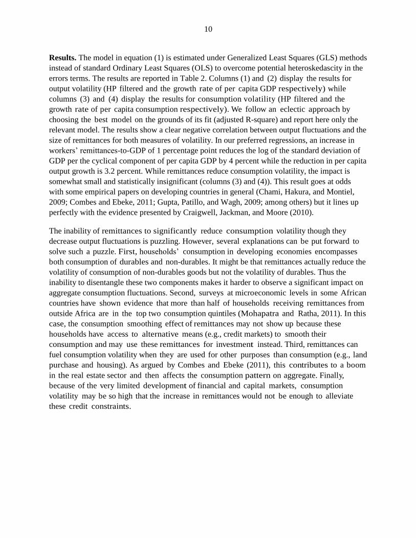
Results. The model in equation (1) is estimated under Generalized Least Squares (GLS) methods

instead of standard Ordinary Least Squares (OLS) to overcome potential heteroskedascity in the

errors terms. The results are reported in Table 2. Columns (1) and (2) display the results for

output volatility (HP filtered and the growth rate of per capita GDP respectively) while

columns (3) and (4) display the results for consumption volatility (HP filtered and the

growth rate of per capita consumption respectively). We follow an eclectic approach by

choosing the best model on the grounds of its fit (adjusted R-square) and report here only the

relevant model. The results show a clear negative correlation between output fluctuations and the

size of remittances for both measures of volatility. In our preferred regressions, an increase in

workers’ remittances-to-GDP of 1 percentage point reduces the log of the standard deviation of

GDP per the cyclical component of per capita GDP by 4 percent while the reduction in per capita

output growth is 3.2 percent. While remittances reduce consumption volatility, the impact is

somewhat small and statistically insignificant (columns (3) and (4)). This result goes at odds

with some empirical papers on developing countries in general (Chami, Hakura, and Montiel,

2009; Combes and Ebeke, 2011; Gupta, Patillo, and Wagh, 2009; among others) but it lines up

perfectly with the evidence presented by Craigwell, Jackman, and Moore (2010).

The inability of remittances to significantly reduce consumption volatility though they

decrease output fluctuations is puzzling. However, several explanations can be put forward to

solve such a puzzle. First, households’ consumption in developing economies encompasses

both consumption of durables and non-durables. It might be that remittances actually reduce the

volatility of consumption of non-durables goods but not the volatility of durables. Thus the

inability to disentangle these two components makes it harder to observe a significant impact on

aggregate consumption fluctuations. Second, surveys at microeconomic levels in some African

countries have shown evidence that more than half of households receiving remittances from

outside Africa are in the top two consumption quintiles (Mohapatra and Ratha, 2011). In this

case, the consumption smoothing effect of remittances may not show up because these

households have access to alternative means (e.g., credit markets) to smooth their

consumption and may use these remittances for investment instead. Third, remittances can

fuel consumption volatility when they are used for other purposes than consumption (e.g., land

purchase and housing). As argued by Combes and Ebeke (2011), this contributes to a boom

in the real estate sector and then affects the consumption pattern on aggregate. Finally,

because of the very limited development of financial and capital markets, consumption

volatility may be so high that the increase in remittances would not be enough to alleviate

these credit constraints.

11

Table2 . Macroeconomic Fluctuations and Remittances

(GLS Estimation)

GDP Consumption

———————— ————————

Variables y ∆y

(1) (2)

c ∆c

(3) (4)

Remittances -4.03* -3.17* -1.61 -1.96

(-2.73) (-2.18) (-0.67) (-0.81) Government size -2.26 -3.07* 3.13 2.63

(-1.71) (-2.71) (1.51) (1.58) Aid volatility 4.12* 3.84* -0.49 -0.75

(2.13) (2.14) (-0.26) (-0.39) Financial development -0.83 -0.77 -1.79* -1.31*

(-1.50) (-1.44) (-2.60) (-2.21) Average GDP -0.13 -0.16

(-1.58) (-1.86) Constant -3.36*** -2.70*** -0.44 0.32

(-12.62) (-12.78) (-0.22) (0.17) Number of observations 25 25 25 25 adj. R-square 0.42 0.43 0.48 0.47

Note: t-student are in parenthesis. (*), (**), and (***) denote significance at 5,1, and 0.1 respectively. ŷ (respectively ĉ) is the cyclical component of the log of per capita GDP (respectively per capita consumption) using the HP filter with a smoothing parameter of 6.25. ∆y (respectively ∆c) is the growth rate of per capita GDP (respectively per capita consumption).

6

6 Using HP filtered data with a smoothing parameter of 100 does not qualitatively affect the results.

12

B. Remittances and Risk Sharing

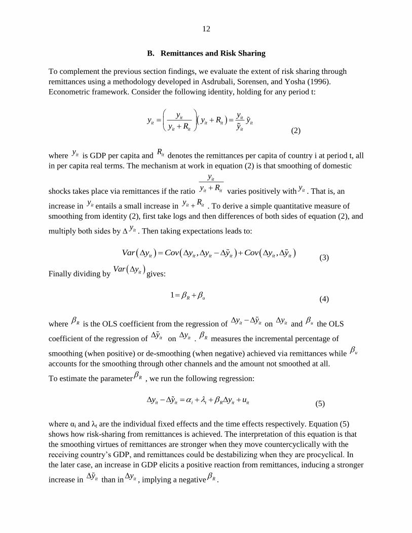
To complement the previous section findings, we evaluate the extent of risk sharing through

remittances using a methodology developed in Asdrubali, Sorensen, and Yosha (1996).

Econometric framework. Consider the following identity, holding for any period t:

it itit it it it

it it it

y yy y R y

y R y

(2)

where ity is GDP per capita and itR

denotes the remittances per capita of country i at period t, all

in per capita real terms. The mechanism at work in equation (2) is that smoothing of domestic

shocks takes place via remittances if the ratio

it

it it

y

y R varies positively with ity

. That is, an

increase in ityentails a small increase in ity

+ itR . To derive a simple quantitative measure of

smoothing from identity (2), first take logs and then differences of both sides of equation (2), and

multiply both sides by ∆ ity. Then taking expectations leads to:

, ,it it it it it itVar y Cov y y y Cov y y

(3)

Finally dividing by itVar y

gives:

1 R u

(4)

where R is the OLS coefficient from the regression of it ity y on ity

and u the OLS

coefficient of the regression of ity on ity

. R measures the incremental percentage of

smoothing (when positive) or de-smoothing (when negative) achieved via remittances while u

accounts for the smoothing through other channels and the amount not smoothed at all.

To estimate the parameter R , we run the following regression:

it it i t R it ity y y u (5)

where αi and λt are the individual fixed effects and the time effects respectively. Equation (5)

shows how risk-sharing from remittances is achieved. The interpretation of this equation is that

the smoothing virtues of remittances are stronger when they move countercyclically with the

receiving country’s GDP, and remittances could be destabilizing when they are procyclical. In

the later case, an increase in GDP elicits a positive reaction from remittances, inducing a stronger

increase in ity than in ity

, implying a negative R .

13

The main results. The results are reported in Table 3. The Hausmann test and the variance

decomposition of ∆y both show that the random effects model is an appropriate specification

for our data. The model in equation (5) with random individual effects is estimated using

different estimation methods: Ordinary Least Squares (OLS), Instrumental Variable (IV), and

System-GMM of Arellano and Bond (2003). IV and GMM estimation techniques are used to

account for potential endogeneity issues where the growth rate of per capita GDP is instrumented

by its own first lag.

The results in Table 3 confirm our cross-section evidence: remittances have a positive and

significant risk-sharing power. They absorb a fraction worth 3.7 to 22 percent of GDP shocks.

The extent to which this number is important depends on the contribution of the other channels

(e.g., capital and credit markets) in absorbing GDP shocks in these economies. Yehoue (2005)

found that remittances together with standard channels (capital and credit markets) absorbed only

15 percent and 13 percent of GDP shocks in the CEMAC and WAEMU CFA zones in 1980–

2000 while development aid especially from France absorbed about 44 percent of shocks.7

Therefore, remittances appear to outweigh capital and credit markets channel in dampening the

effects of macroeconomic shocks. In addition, given the potential effect of remittances on

promoting financial development (Gupta, Patillo, and Wagh, 2009; Combes and Ebeke, 2011;

World Bank, 2006, 2011), their cumulated direct and indirect stabilizing effects on business

cycle fluctuations could be significantly higher than thought. Moreover, our quantitative findings

represent the lower bound values of the effective impact of remittances in African countries as

the quality and coverage of data in general and on remittances in particular leave much to be

desired. Transfers through informal channels, misreporting in the receiving countries, and

misclassification of remittances into other revenues (exports revenues, tourism receipts,

nonresident deposits, or FDI, World Bank, 2011) are among the main reasons for the

underestimation of remittances in developing countries, particularly African economies.

7 CEMAC stands for Economic and Monetary Community of Central Africa and WAEMU is the West African

Economic and Monetary Union.

14

Table 3. Remittances and Risk Sharing

GLS GLS IV IV GMM GMM

(1) (2) (3) (4) (5) (6)

R (%) 3.74 3.70 16.7 21.56 14.81 9.35

(1.85) (1.95) (8.97) (12.31) (7.7) (4.75)

Time fixed effects No Yes No Yes No Yes

Number of observations 644 644 619 619 644 644

Sargan Test Prob > χ2 0.81 0.33

Hansen Test Prob > χ2 0.77 0.64

AR(1): p–value 0.009 0.008

AR(2): p–value 0.226 0.241

Note: Standard errors are in parenthesis.

IV. A SMALL OPEN ECONOMY MODEL WITH REMITTANCES

The objective of this section is to provide a theory supporting the preceding empirical results

(Section 2.1). In particular, we probe the theoretical transmission channels through remittances

affect macroeconomic fluctuations consistent with the above empirical results. We argue that the

absence of a reduction in consumption volatility in response to an increase in remittances stems

from the excess volatility of consumption with respect to GDP, which itself results from

underdeveloped financial and limited access to capital markets. We use the standard one-good

neoclassical small open economy DSGE model developed in Garcia-Cicco, Pancrazi, and Uribe

(2010) where financial frictions play a leading role in generating an excess consumption

volatility.

A. The Theoretical Model

We briefly review the main features of the model. A more detailed description of this model can

be found in Jidoud (2012) and references mentioned above.

Preferences. The economy is populated by a representative household whose objective is to

maximize its discounted lifetime utility:

1

,t

t t t

t

E U c N

(6)

where β ∈ [0, 1) is the discount factor, ct is current consumption, U(.) is a period utility function,

and Et (.) is the conditional expectation operator on the information available to the household up

to period t. The objective of the household is to maximize the above utility subject to the

sequence of per period budget constraints given in (11).

15

Two utility specifications are called to compete in this setup. The first is the KPR preferences

(King, Plosser, and Rebelo, 1988) given by

1

(1 ) 1,

1

t t

t t

c NU c N

(7)

and the second is the so called GHH preferences following Greenwood, Hercowitz, and Huffman

(1988)

1

1

,1

tt

t t

Nc

U c N

(8)

ω > 1 governs the intertemporal substitution of labor supply while σ ≥ 1 stands for the inverse of

the intertemporal elasticity of consumption.

The motivation behind confronting the two preferences specifications is the size of the wealth

effect they generate. They indeed represent different levels of constant wealth effect for a given

elasticity of labor supply. GHH preferences (8) have the property that labor supply is

independent of wealth and is accordingly determined independently from the consumption level

of the household. Thus the wealth effect is zero. On the other hand KPR preferences generate a

sizeable wealth effect which, everything else equal, would reduce the labor supply of the

households in response to a shock that induces an increase in the marginal utility of wealth. In

addition, GHH preferences are widely used in the business cycles analysis of developing

countries on the grounds that they help the small open economy models reproduce the stylized

business cycle facts of open economies, in particular, countercyclical trade balances (Mendoza,

1991; and Garcia-Cicco, Pancrazi, and Uribe, 2010; among others). Therefore comparing the

performances of these two specifications is of particular interest for this literature.

Technology. The economy produces one single good using a Cobb–Douglass production

function with constant return to scale as follows:

1

t t t tY a AK N (9)

where Yt denotes output in period t, Kt denotes capital in period t, Nt denotes labor input in

period t, A¯ > 0 is a scale parameter that pins down the level of output. We assume that

fluctuations in output are solely driven by a transitory productivity shock at which follows a

first-order autoregressive process, that is,

2

1ln( ) (1 )ln( ) ln( ) , ~ (0, ).a a

t a a t t t aa A a N (10)

where a < 1 denotes the persistence of the shock.

16

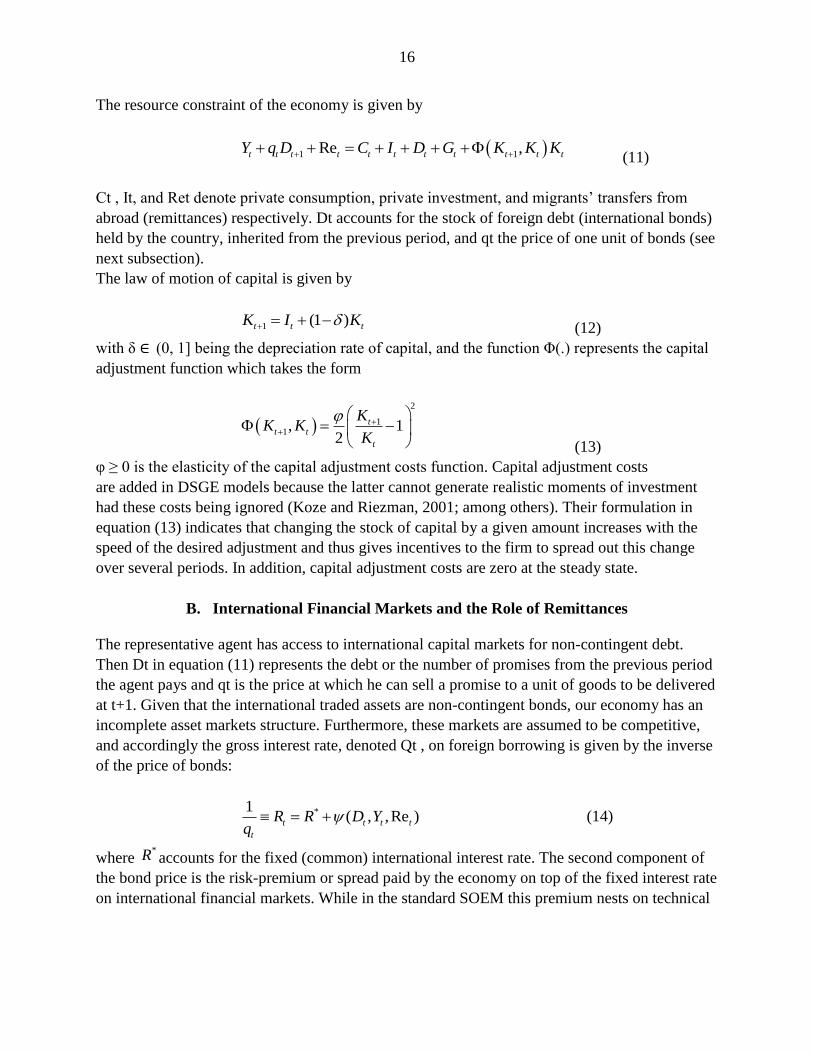
The resource constraint of the economy is given by

1 1Re ,t t t t t t t t t t tY q D C I D G K K K

(11)

Ct , It, and Ret denote private consumption, private investment, and migrants’ transfers from

abroad (remittances) respectively. Dt accounts for the stock of foreign debt (international bonds)

held by the country, inherited from the previous period, and qt the price of one unit of bonds (see

next subsection).

The law of motion of capital is given by

1 (1 )t t tK I K (12)

with δ ∈ (0, 1] being the depreciation rate of capital, and the function Φ(.) represents the capital

adjustment function which takes the form

2

11, 1

2

tt t

t

KK K

K

(13)

φ ≥ 0 is the elasticity of the capital adjustment costs function. Capital adjustment costs

are added in DSGE models because the latter cannot generate realistic moments of investment

had these costs being ignored (Koze and Riezman, 2001; among others). Their formulation in

equation (13) indicates that changing the stock of capital by a given amount increases with the

speed of the desired adjustment and thus gives incentives to the firm to spread out this change

over several periods. In addition, capital adjustment costs are zero at the steady state.

B. International Financial Markets and the Role of Remittances

The representative agent has access to international capital markets for non-contingent debt.

Then Dt in equation (11) represents the debt or the number of promises from the previous period

the agent pays and qt is the price at which he can sell a promise to a unit of goods to be delivered

at t+1. Given that the international traded assets are non-contingent bonds, our economy has an

incomplete asset markets structure. Furthermore, these markets are assumed to be competitive,

and accordingly the gross interest rate, denoted Qt , on foreign borrowing is given by the inverse

of the price of bonds:

*1( , ,Re )t t t t

t

R R D Yq

(14)

where *R accounts for the fixed (common) international interest rate. The second component of

the bond price is the risk-premium or spread paid by the economy on top of the fixed interest rate

on international financial markets. While in the standard SOEM this premium nests on technical

17

necessities, in our setup it acts as a reduced form of a financial friction governing the dynamic

effects of aggregate fluctuations and the transmission of financial shocks.8 Therefore the

parameter ψ reflects the tightness or the sensitivity of these financial frictions to different

macroeconomic variables (GDP, debt, remittances). In dealing with this friction, we adopt two

modeling assumptions. First we assume the country risk premium is determined by the

indebtedness of the economy with respect to its output. So that (14) is given by

* exp( ) 1tt

t

D DR R

Y Y

(15)

where variables with bars are the steady state values. In this specification, the level of the

country’s indebtedness has a positive effect on the borrowing cost. The higher the debt relative to

GDP the higher is the interest rate paid by the country because investors will fear the probability

of default of the country (Garcia–Cicco, Pancrazi, and Uribe, 2010; Ozbilgin, 2010; for a closer

formulation). In a second specification we assume the flow of remittances has some impact on

the country’s borrowing costs. Formally (14) become

* exp( ) 1

Re Re

tt

t t

D DR R

Y Y

(16)

This modeling assumption is underpinned by the empirical evidence that remittances lessen the

remittances-dependent countries’ borrowing cost on international capital markets and enhance

their creditworthiness. Furthermore, some African countries have used remittances as securitized

assets to raise funds on international financial markets at low cost and longer maturities (Ratha,

De, and Mohapatra, 2011; Afreximbank, 2005). Evidence about the ability of remittances to ease

access to financial markets is a well-established fact in most African economies.

V. QUANTITATIVE ANALYSIS

The model is log-linearized around the deterministic stationary steady state. The structural

parameters of the model are calibrated following the business cycle literature on developing

economies and mostly African countries whenever possible.

Calibration. We consider our panel of countries to form a representative African economy. The

parameters of the model are calibrated following the existing work and according to the annual

frequency of the data. But their choice is evaluated with respect to the model’s ability to mimic

some features of this economy as observed in 1980–2005. It is worth noting that the calibration

8 In standard SOEM, this trick is introduced to have a stationary model (see Schmitt-Grohe and Uribe,

2003).

18

for some of the parameters entails great uncertainty because we lack thorough, reliable studies on

African countries on these parameters. To overcome this problem, we later provide some

sensitivity analysis on these parameters. We set the discount factor β = 0.98, which implies an

interest rate level equal to 2.04 percent. The share of capital income to total income of the

economy α is set to 0.33. The inverse of the intertemporal elasticity of consumption, σ, is set to

5 following Arellano and others (2009). All these values are pretty standard in the literature of

business cycles. The persistence and the standard deviation of the total factor productivity (TFP)

are to 0.9271 and 0.0126 respectively. The annual depreciation rate of capital δ is equal to 0.15,

while the capital adjustment cost parameter φ = 5. The depreciation rate is set to 0.15 and its

relatively high value reflects the higher depreciation of capital stock in developing countries (Bu,

2006). The relatively high value of the capital adjustment cost parameter φ reflects the difficulty

of adjusting capital in developing economies (Tybout, 2000; Bigsten and others, 2005). We set ω

(one plus the labor supply elasticity) equal to 1.5, a value close to that chosen by Mendoza

(1991) for a small open economy case.9 The debt-to-GDP ratio is equal to 0.80, a value fairly

consistent with the indebtedness size of African economies.

The model is finally simulated for different values of the elasticity of the risk premium. We

specifically consider three values for this parameter: 1, 2.5, and 7.5, with a higher value

reflecting tight borrowing constraints or the sensitivity of bond prices to the different arguments

in the risk-premium function. Table 3 summarizes this calibration.

The model is solved by varying the steady state level of workers’ remittances-to-GDP ratio over

three values: 0, 0.0378 and 0.0756. The empirical mean (of the countries included in the

regression) which we consider, the steady state value is 3.78 percent. The performances of the

model with respect to the data are evaluated by computing the semi-elasticity, εσx of the

generated volatilities around the steady state value of the remittances-to-GDP ratio. Formally

speaking this semi-elasticity (consistent with the empirical model) is given by

log( )

Rex

x

(17)

9 Empirical work is scarce on labor markets in African economies capable of allowing us to have a clear cut

value on labor elasticity. However the value set here could be justified the existence of a sizeable informal

sector in these economies and high unemployment rate.

19

Table 4. Calibrated Parameters

Parameters Description Value

β Discount factor 0.95

α Capital to output ratio 0.33

σ Inverse of intertemporal elasticity of consumption 5

δ Depreciation rate of capital 0.15

ω One plus the inverse of labor supply elasticity 1.5

φ Capital adjustment costs 5

ρ Persistence of TFP shock 0.9271

σ Standard deviation of TFP shock 0.0126

D/Y Debt-to-GDP ratio 0.80

ψ The debt price elasticity {1, 2.5, 7.5}

A. The Role of Wealth Effect on Labor Supply

The model is simulated under the world interest rate specification (15) in which we assume the

size of remittances have no direct effects on the country’s risk premium. Table 5 reports the

results. Column (1) displays all the characteristics of the data for comparison while columns

(2)–(4) report the results using KPR preferences. Columns (5)–(7) deal with GHH preferences.

It is worth noting that the model replicates well the business cycle facts in these economies. In

particular, the consumption to output volatility predicted by the model is the actual one

especially with GHH preferences and tight borrowing constraints.

How does the model perform in terms of the effects of remittances on macroeconomic

fluctuations? In columns (2)–(4), consumption volatility decreases, but output volatility increases

as the size of remittances increases. Hence remittances have stabilizing effects on consumption

and destabilizing effects on output. Unlike KPR preferences, GHH preferences give negative

elasticities for both consumption and output. The stabilizing impact of remittances on output

becomes stronger (higher elasticity in absolute value) as the risk-premium sensitivity ψ increases

but the elasticity of consumption volatility decreases (in absolute value) though it remains

negative for all degree of financial tightness. For example, when ψ = 1, a 1 percent increase in

the remittances-to-GDP ratio increases (decreases) output (consumption) volatility by 0.39 (0.59)

percentage point with KPR preferences. These numbers are 0.03 and 0.80 in the case of GHH

preferences. But when the risk premium strongly responds to the indebtedness ratio, an increase

of 1 percent in the remittances size reduces both output and consumption volatility by 0.3 and

0.24 percentage points. In summary, besides their ability to generate plausible business cycle

facts, GHH preferences are more consistent with our empirical finding: increasing the size of

remittances cushions both output and consumption instabilities with the effect on output

fluctuations being much more pronounced.

20

Table 5. Model Predictions and the Wealth Effect

Data KPR preferences GHH preferences

———————————

———————————

ψ = 1 ψ = 2.5 ψ = 7.5 ψ = 1 ψ = 2.5 ψ = 7.5

Output

εσy

εσ∆y

Consumption εσc

εσ∆c

-4.03 0.39 0.36 0.45 0.03 -0.03 -0.30

-3.17 0.34 0.33 0.36 -0.07 -0.20 -0.53

-1.60

-0.59

-0.55

-0.53

-0.80

-0.56

-0.24

-1.96 -0.60 -0.56 -0.53 -0.90 -0.70 -0.47

Relative volatility σc/σy 1.57 1.34 1.76 2.27 1.25 1.46 1.54

σ∆c/σ∆y

Autocorrelation

1.62 1.27 1.64 2.10 1.17 1.31 1.37

ρy 0.37 0.18 0.34 0.54 0.22 0.39 0.58

ρ∆y 0.06 0.21 0.43 0.70 0.32 0.56 0.77

ρc 0.42 0.07 0.05 0.01 0.11 0.14 0.17

ρ∆c

Correlation

0.00 -0.03 -0.07 -0.12 0.10 0.12 0.18

ρy,c 0.45 0.97 0.86 0.46 0.98 0.90 0.60

ρ∆y,∆c 0.39 0.96 0.85 0.49 0.97 0.90 0.67

Note: ŷ and ĉ account for the cyclical component of the HP filtered logs of per capita GDP and private consumption while ∆y and ∆c are the growth rates of the same variables. The model is simulated with completely exogenous remittances. That is, Ȓt = 0. The steady-state level of remittances takes the values 0, 0.0378 and 0.0756. The autocorrelations and the relative volatilities from the model are taken when the model is simulated at the empirical average of the steady state size of remittances to GDP ratio: 0.0378.

The key channel driving the difference between the two cases is the wealth effect generated by

the two preferences. In the GHH preferences, the wealth effect on labor supply is nil whereas it

is strictly positive for KPR for a given level of labor elasticity. Because of this wealth effect,

labor supply decreases in the case of KPR preferences following an increase in the size of

remittances. Households consume more leisure and then the steady state level of employment is

reduced. The reduction in the steady state employment increases the elasticity of labor supply

and deepens the response of hours and output following a positive TFP shock.10

This is why

output volatility increases following a positive TFP shock for example (see Chami and others,

2008, for a graphical illustration of this effect: technology shocks plus income effect). When

10 The elasticity of labor supply is given by

1

1GHH

in the GHH case and by

1KPR

N

N

in the KPR case.

(1) (2) (3) (4) (5) (6) (7)

21

households’ preferences are for GHH, their labor supply decision is no longer affected by their

income level but only by their wages. In response to a positive TFP shock labor supply increases

but does not affect the elasticity of labor supply contrary to the case with KPR preferences. The

constant elasticity of labor supply avoids output to respond strongly to TFP shocks. The

observed decline in output volatility, although small, comes from a composition effect. Because

consumption becomes less and less volatile, GDP fluctuations are moderated as the size of

remittances becomes larger.

Figures 4 and 6 plot the impulse responses of different aggregates after a TFP shock for different

levels of remittances-to-GDP ratio for KPR and GHH preferences, respectively. It turns out that

an increase in remittances does not significantly affect the reaction of output, nor of

consumption, in response to a TFP shock in KPR. However, it makes both output and

consumption responses less strong for GHH.

Why does consumption volatility decrease in both cases? Such a result stems from the reduction

of the private consumption multiplier. Indeed an increase of remittances increases the steady

state consumption-output ratio. This decouples consumption from output dynamics as

consumption responds less to TFP shocks and income fluctuations. Yet this mechanism is not the

only one at work. An additional channel driving the reduction of consumption volatility is the

composition effect. Because remittances are not volatile themselves, and we are increasing the

size of the non-volatile component of consumption, the volatility of consumption decreases.

The above investigation has shed light on the wealth effect on labor supply as the main

mechanism through which remittances deepen or dampen macroeconomic fluctuations. Further-

more, these effects are stronger in economies in which households have very limited access to

financial markets. Unfortunately, this channel fails to generate a strong reduction in

macroeconomic volatility as observed in our empirical investigation. For such a channel to

generate sizeable smoothing effects, the model needs a strong propagation mechanism.

B. Remittances and Financial Frictions

In the previous subsection, increasing the size of remittances buffered macroeconomic

fluctuations in an environment where households’ preferences exhibit no wealth effect and they

face strong financial frictions. To improve the model’s performances in generating a sizeable

reduction in macroeconomic volatility, we now allow remittances to have negative effects on the

risk premium. We thus simulate the model using the specification (16) for the risk premium,

which entails a loosening effect of remittances on financial constraints. The results are displayed

in Table 6. The predictions of the model are qualitatively identical to those of the baseline setup.

Remittances have a negative effect on both output and consumption volatility when the wealth

effect in the preferences is killed off (GHH case) while they deepen output volatility when the

income effect is allowed (KPR case). However, unlike the previous case, the semi-elasticities in

Table 5 are higher in absolute value. That is, the reduction in both output and consumption

fluctuations is more substantial. For example, when the risk-premium sensitivity is 7.5, a

22

1 percent increase in the size of remittances reduces output (consumption) instability by

1.66(1.56) percentage point when preferences are GHH type. In addition, the impact on volatility

is stronger as financial constraints become tighter. The labor supply mechanism at work in the

previous case still prevails. But the mechanism is much stronger now as more remittances imply

greater possibilities to accumulate debt and decouple both consumption and output from TFP

shocks. As can be seen in Figures 5 and 7, an increase in remittances entails a smaller response

of output and consumption after a TFP shock. The dampening in these reactions is much stronger

in GHH preferences. Moreover, the increase in output after a shock lasts longer in this case,

affording households more income over time. Topping up the risk premium with remittances

proves to be a powerful propagation mechanism, inducing the smoothing effect of remittances.

In this new setup, an increase in the size of remittances implies a reduction in the costs of

borrowing on international financial markets. This effect transmits into a more stable debt level

and accordingly a reduction in the trade balance fluctuations. Hence reducing the risk premium

remittances contribute to the stabilization of output and consumption as households get easier

access to financial markets.

The bottom line of this analysis is that the stabilizing effect of remittances is stronger in an

environment where financial frictions are tight, that is, borrowing constraints are permanently

binding. This finding is quite intuitive. In an economy in which individuals can easily save

and/or borrow, the marginal value of a unit of remittances is small; and remittances may have no

effect on macroeconomic volatility. However, in an economy in which the options for saving and

borrowing are limited, remittances constitute a direct source of income but also an asset that

helps alleviate these borrowing constraints. This finding has some empirical support in the

papers of Gupta, Patillo, and Wagh (2009) and Combes and Ebeke (2011), among others. This

result also lines up with Ahamada and Coulibaly (2011) who find the smoothing effect of

remittances in sub-Saharan African countries to be nonlinear and higher depending on the level

of financial development.

23

Table 6. Model Predictions and Financial Development

Output

εσy

εσ∆y

Consumption εσc

εσ∆c

-4.03 0.57 0.60 0.25 0.00 -0.36 -1.66

-3.17 0.51 0.48 0.13 -0.23 -0.71 -1.93

-1.60

-0.98

-1.07

-1.09

-1.25

-1.34

-1.56

-1.96 -0.97 -1.07 -1.08 -1.36 -1.51 -1.20

Relative volatility σc/σy 1.57 1.30 1.71 2.24 1.23 1.43 1.55

σ∆c/σ∆y

Autocorrelation

1.62 1.25 1.60 2.08 1.16 1.30 1.38

ρy 0.37 0.17 0.32 0.54 0.21 0.37 0.58

ρ∆y 0.06 0.20 0.41 0.69 0.31 0.54 0.76

ρc 0.42 0.07 0.05 0.02 0.11 0.14 0.17

ρ∆c

Correlation

0.06 -0.03 -0.06 -0.11 0.10 0.13 0.17

ρy,c 0.45 0.97 0.88 0.50 0.98 0.91 0.63

ρ∆y,∆c 0.39 0.97 0.87 0.52 0.97 0.91 0.69

Note: y and c account for the cyclical component of the HP filtered logs of per capita GDP and private consumption while ∆y and ∆c are the growth rates of the same variables. The model is simulated with completely exogenous remittances. That is, Rt = 0. The steady-state level of remittances takes the values 0, 0.0378, and 0.0756. The autocorrelations and the relative volatilities from the model are taken when the model is simulated at the empirical average of the steady-state size of remittances to GDP ratio: 0.0378.

VI. SENSITIVITY ANALYSIS

We assess the robustness of the previous results alongside the following dimensions: the

discount factor, the degree of risk aversion, and the capital adjustment cost parameter. All the

following results are obtained by simulating the model under specification (16) of the world

interest rate.

The elasticity of labor supply. In the baseline setup, the parameter ω, which governs the labor

supply elasticity, was taken to be equal to 1.5, equal to a labor elasticity of 2. This parameter is

subject to an endless debate in developing countries as the study of labor markets in these

countries is at its infancy on account of the unavailability of adequate household data and the

attention being more focused on surplus labor and underemployment. We check the robustness

of our results along different values (1.2 and 2) of this parameter but only for GHH preferences

because these are the only ones concerned with this parameter. The results are presented in Table

6. We see that the higher the elasticity of labor supply (low ω), the stronger is the stabilizing

Data KPR Preferences GHH Preferences

———————————

——————————— ψ = 1 ψ = 2.5 ψ = 7.5 ψ = 1 ψ = 2.5 ψ = 7.5 (1) (2) (3) (4) (5) (6) (7)

24

effect of remittances on output and consumption. Furthermore, in such a setting, the results are

more qualitatively consistent with the empirical facts, that is, the stabilizing role of remittances is

more pronounced on output than on consumption. When the labor supply elasticity is low, the

semi-elasticities of output and consumption are negative, but the effect is less pronounced for

output. Clearly this analysis brings out the role of labor market characteristics in shaping the

impact of remittances in business cycles in developing countries. In countries where workers

strongly adjusted their labor supply in response to wage variations, remittances are expected to

significantly cushion the resulting fluctuations in output and consumption. On the contrary, when

the labor supply elasticity is relatively low, the stabilizing effect of remittances is limited.

Table 7. Model Predictions as ω Changes

ω = 1.2

Output

εσŷ

Consumption

εσĉ

ω = 2

Output

εσŷ

Consumption

εσĉ

Data GHH Preferences

———————————

ψ = 1 ψ = 2.5 ψ = 7.5

(1) (2) (3) (4)

-4.03 -0.09 -0.81 -2.27

-1.60 -1.04 -1.20 -1.81

-4.03 0.02 -0.18 -1.20

-1.60 -1.40 -1.55 -1.79

25

The discounting dimension. In the benchmark setup we assume the representative

household discounts time at a rate 0.98, which corresponds to an annual real interest rate of

2.04 percent. While this corresponds to commonly practiced world interest rate for developing

countries, we are greatly interested in assessing the validity of our results in the hypothesis the

household is more or less patient compared to the baseline setup. The degree of patience of

households may undermine the effects of remittances because it determines the

consumption/savings decisions of households.

Table 7 shows the results for two values of the discount rate. The figures are quantitatively and

qualitatively in line with those of the benchmark model. Remittances have a negative effect on

macroeconomic fluctuations when they are poured into economies with low financial

development. The more impatient are the households (a lower discount factor) the stronger is the

smoothing effect of remittances. The impatience of households (β = 0.92) results in an important

smoothing behavior because of the higher interest rates faced by the households. A higher fixed

interest rate is an additional financial constraint and thus fuels the effect of remittances on

macroeconomic fluctuations.

Table 8. Model Predictions as β Changes

β = 0.99

Output

εσŷ

Consumption

εσc

β = 0.92

Output

εσŷ

Consumption

εσc

Data KPR Preferences GHH Preferences

——————————— ———————————

ψ = 1 ψ = 2.5 ψ = 7.5 ψ = 1 ψ = 2.5 ψ = 7.5

(1) (2) (3) (4) (5) (6) (7)

-4.03 0.54 0.56 0.20 -0.002 -0.35 -1.61

-1.60 -0.96 -1.06 -1.09 -1.16 -1.22 -1.39

-4.03 0.71 0.81 0.49 0.02 -0.37 -1.79

-1.60 -1.03 -1.11 -1.06 -1.61 -1.87 -2.27

26

Intertemporal substitution. It is well known that the strength of the intertemporal substitution

(the curvature of the utility function) carries the consumption-smoothing objective of the

households. The higher the substitution is, the more intense is the consumption-smoothing

objective and thus the greater will be the intertemporal reallocation of resources in the face of a

productivity shock. In our benchmark analysis the risk-aversion parameter was set to 5, a value

widely used in standard RBC analysis for developing countries (Arellano and others, 2009).

Nevertheless, when it comes to developing countries, scarcity of reliable empirical studies on

this issue makes it difficult to stick to specific values for these parameters. We thus assess the

sensitivity of our results along this intertemporal substitution dimension. We choose a small

value (σ = 1) and a higher one (σ = 10).

The results shown in Table 8 are in line with the baseline ones. The stabilizing effect of

remittances is higher for a higher degree of intertemporal substitution because of households’

desire to smooth the consumption path. A higher degree of intertemporal substitution pushes the

households to reallocate the additional resources from remittances for future consumption. In so

doing, households opt for smoother income and consumption paths. When the intertemporal

substitution is small, households’ desire to postpone present consumption to future periods is

low, and this lessens the power of remittances to reduce consumption fluctuations.

Table 9. Model Predictions as σ Changes

σ = 1

Output

εσŷ

Consumption

εσĉ

σ = 10

Output

εσŷ

Consumption

εσĉ

Data KPR Preferences GHH Preferences

——————————— ———————————

ψ = 1 ψ = 2.5 ψ = 7.5 ψ = 1 ψ = 2.5 ψ = 7.5

(1) (2) (3) (4) (5) (6) (7)

-4.03 0.73 0.67 0.80 0.01 -0.21 -1.32

-1.60 -1.13 -1.10 -0.83 -1.24 -1.32 -1.42

-4.03 0.52 0.52 0.10 -0.01 -0.41 -1.67

-1.60 -0.93 -1.05 -1.12 -1.31 -1.45 -1.83

27

Capital Adjustment Costs. Capital adjustment costs are generally included in SOEM to

avoid important swings in investment. The baseline value of 5 is reasonable given the

arguments exposed in the previous section. As such, higher adjustment costs may by

themselves reduce the volatility of investment and accordingly reduce output volatility

through a composition effect. To see the extent to which our results rely on choice of the

value of this parameter, we reevaluate the model’s performances with two values around the

baseline value: 2 and 10.

The results in Table 9 show that our central findings are not challenged by the capital

adjustment costs parameter. Higher remittances induce a decrease in both volatilities of

output and consumption although the decrease is now more pronounced for consumption.

Surprisingly, the reduction in macroeconomic volatility is more substantial when the

adjustment costs are low. The mechanism might be that lower adjustment costs allow

households to easily invest their remittances, which increases income over time and affords

more possibilities to cushion macroeconomic shocks.

Table 10. Model Predictions as φ Changes

φ = 2

Output

εσŷ

Consumption

εσĉ

φ = 10

Output

εσŷ

Consumption

εσĉ

Data KPR Preferences GHH Preferences

——————————— ———————————

ψ = 1 ψ = 2.5 ψ = 7.5 ψ = 1 ψ = 2.5 ψ = 7.5 (1) (2) (3) (4) (5) (6) (7)

-4.03 0.42 0.27 -0.09 -0.20 -0.66 -1.58

-1.60 -0.93 -1.03 -1.10 -1.35 -1.52 -1.96

-4.03 0.67 0.84 0.69 0.10 -0.06 -1.48

-1.60 -1.01 -1.10 -1.06 -1.28 -1.41 -1.62

In light of what precedes, it is worth noting that our central finding, that is, the stabilizing

effects of remittances are more pronounced in economies with fewer options for

savings/borrowing and no wealth effect on labor supply, is robust to various alterations of

different structural parameters.

28

VII. CONCLUSION

How effective are remittances in stabilizing aggregate fluctuations? How much of shocks is

absorbed through migrants’ transfers? What are the mechanisms and channels through which

remittances affect business cycle volatility? These are questions at the forefront of public

and policy debate on the role of migration and remittances in developing countries. This

paper responds to these questions by focusing on African economies. Consistent with the

existing similar work on other countries, our empirical analysis suggests that larger

remittances tend to reduce consumption and output volatility, that is, countries with higher

remittances-to-GDP ratio display lower business cycle fluctuations. Nevertheless, the

puzzling result is that the reduction in consumption volatility is less pronounced than for

output volatility. Our interpretation of this finding is that given the relatively high volatility

of consumption with respect to output, the level of remittances falls short of significantly

reducing consumption volatility. Moreover, a portion worth 3.7 to 22 percent of GDP shocks

is absorbed via remittances, suggesting the risk-sharing power of these transfers.

The main contribution of the paper to literature is the investigation of the theoretical channels

and mechanisms through which remittances affect macroeconomic volatility using a general

equilibrium framework. This theoretical analysis shows that the stabilization impact of

remittances essentially hinges on two channels: (i) the size of the negative wealth effect on labor

supply induced by remittances and, (ii) the strength of financial frictions and the ability of

remittances to alleviate these frictions. The first channel implies that labor supply may decrease

following an increase in remittances, lowering output and increasing its response to shocks. The

second channel suggests remittances are more stabilizing in countries with a shallow financial

and banking sector and when remittances induce financial sector development by providing a

greater access to financial markets to their recipients (which can improve their creditworthiness

scores). This later finding underscores the need for recipient countries to promote financial

development so as to channel remittances through the financial system and help the poor have

greater access to credit. This paper is among the first attempts to bring about a clear

understanding of the transmission mechanism of remittances into the real economy. It

bridges the gap between the burgeoning empirical work on the issue and the underlying

theoretical mechanism. The paper points to the direction of labor markets and financial

frictions as the two channels through which remittances exert their effects on business cycles

in developing countries. Labor markets modeling issues and international financial frictions

in developing countries have to be seriously considered when trying to understand the

macroeconomic effect of remittances. This should be part of our future research agenda.

29

References

Adams, Jr., R.H., and J. Page (2005) “Do international migration and remittance reduce

poverty in developing countries?”, World Development, 33, pp. 1645–1669.

Afreximbank (2005), Annual Report, http://www.afreximbank.com.

Agenor, P., McDermott, C., and Prasad, E. (2000) “Macroeconomic fluctuations in developing

countries: some stylized facts”, World Bank Economic Review, 14, pp. 251–285.

Aguiar, M., and G. Gopinath, (2007) “Emerging markets business cycles: the cycle is the

trend”, Journal of Political Economy, 115, pp. 69–102.

Ahamada, I., and Coulibaly, D. (2011), “How does financial development influence the

impact of remittances on growth volatility?”, Economic Modelling, 28, pp. 2748–2760.

Ahmed, A., and Suardi, S. (2009) “Macroeconomic volatility, trade and financial

liberalization in Africa,” World Development, 37, pp. 1623-1636.

Andres, J., R. Domenech and A. Fatas (2008) “ The stabilizing role of government size”,

Journal of Economic Dynamics and Control, 32, pp. 571–593.

Arellano, C., A. Bulir, T. Lane and L. Lipschitz, (2009) “The dynamic implications of

foreign aid and its variability” Journal of Development Economics, 88, pp. 87–102.

Asdrubali, P., B. E. Sorensen, and O. Yosha (1996), “Channels of Interstate Risk Sharing:

United States 1963-1990”, Quaterly Journal of Economics, 111, pp. 1081-1110

Azam, J-P., and F. Gubert (2005) “Those in Kayes: the effects of remittances on their

recipients in Africa”, Revue Economique, 56, pp. 1331–1358.

Bekaert, G., Harvey, C., and Lundblad, C. (2006) “Growth volatility and financial

liberalization”, Journal of International Money and Finance, 25, pp. 370-403.

Bigsten, A., P. Collier, S. Dercon, M. Fafchamps, B. Gauthier, J.W. Gunning, R. Oostendorp,

C. Patillo, M. Soderbom and F. Teal (2005) “Adjustment costs and irreversibility as

determinants of investment: evidence from African manufacturing”, Contribution to

Economic Analysis and Policy, Vol 4.

30

Bourdet, Y., and H. Falck (2006) “Emigrants remittances and Dutch Disease in Cape

Verde”, International Economic Journal, 20, pp. 267-84.

Bu, Y. (2006) “Fixed capital stock depreciation in developing countries: some evidence

from firm level data”, Journal of Development Studies, 42, pp. 881–901.

Bugamelli, M., and F. Paterno (2009a) “Do workers’ remittances reduce the probability of

current account reversals”, World Development, 37(12), pp. 1821-1838.

Bugamelli, M., and F. Paterno (2009b) “Output growth volatility and remittances”,

Economica, pp. 121.

Bulir, A., and A.J. Hamann (2003) “Aid volatility: an empirical assessment”, IMF Staff

Papers, 50, 64-89.

Chami, R., A. Barajas, T. Cosimano, C. Fullenkamp, M. Gapen and P. Montiel and Hakura

(2008) “Macroeconomic consequences of remittances”, IMF occasional paper, 259.

Chami, R., Hakura, D., and Montiel, P. (2009), “Remittances: An automatic output

stabilizer?” IMF working paper no. 09/91.

Combes, J-L., and C. Ebeke, (2011) ”Remittances and households consumption volatility

in developing countries”, World Development Issues, 9, pp. 1076–1089.

Craigwell, R., M. Jackman and W. Moore, (2010) ”Economic volatility and

remittances”, In- ternational Journal of Development Issues, 9, pp. 25–42.

Durdu and Sayan (2010) “Emerging Market Business Cycles with Remittance

Fluctuations,” IMF Staff Papers, Palgrave Macmillan, vol. 57, pp. 303–325.

Freund, C., and C. Spatafora (2005) “Remittances: transaction costs, determinants, and

infor- mal Flows”, World Bank policy research working paper no. 3704, Wasgington,

D.C.

Garcia-Cicco, J., Pancrazi, R. and Uribe, M., (2010) “Real business cycles in emerging

economies?”, American Economic Review, 100, pp. 2510–2531.

Greenwood, J., Hercovitz, Z. and Huffman, G.W., (1988) “Investment, capacity utilization,

and the real business cycle”, American Economic Review, 78, pp. 402-417.

Gupta, S., Patillo, C., and Wagh, S. (2009) “Effect of remittances on Poverty and finacial

development in subsahran africa”, World Development, 37, pp. 104–115.

Jidoud, Ahmat (2012), "The Sources of Macroeconomic Fluctuations in Sub-Saharan African

Economies: An application to Côte d'Ivoire,"TSE Working Papers 12-346, Toulouse School of

Economics (TSE).

31

King, R., C.I. Plosser and S.T. Rebelo (1988) “Production, growth and the business cycles:

The basic neoclassical model”, Journal of Monetary Economics, 21, pp. 195–232.

Kose, M. A. and Riezman, R., (2001) “Trade shocks and macroeconomic fluctuations in

Africa”, Journal of Development Economics, 65, pp. 55–80.

Loayza, N.V., R. Ranciere, L. Serven and J. Vantura, (2007) “Macroeconomic volatility

and welfare in developing economies ”, World Bank Economic Review, 21, pp. 343–357.

Mendoza, E.G., (1991) “Real business cycles in a small open economy”, American

Economic Review 81 , pp. 797-818.

Mohapatra, S. and D. Ratha (2011) “Remittances markets in Africa”, The World bank,

Wash- ington D.C, pp. 3–88.

Ozbilgin, H.M (2010) “ Financial market participation and the developing country business

cycle”, Journal of Develoment Economics, 92, pp. 125–137.

Pallage, S. and M. Robe (2001) “Foreign aid and the business cycle”, Review of

International Economics, 9, pp. 641-675.

Pallage, S., M. Robe and C. Berube (2007) “The potential of foreign aid as insurance”, IMF

Staff Papers, 53, pp. 453-475.

Ratha, D., (2007), “Leveraging remittances for development, Policy Brief (June), Migration

Policy Institute,Washington, DC.

Ratha, D., P.K. De and S. Mohapatra (2011) “Shadow sovereign ratings for unrated

developing dountries”, World Development, 39, pp. 295–307.

Schmitt-Grohe, S., Uribe, M., (2003) “Closing small open economy models” Journal of

Inter- national Economics, 61, pp. 163-185.

Tybout, J. (2000) “Manufacturing firms in developing countries: how well do they do, and

why?”, American Economic Review, 38, pp. 11-44.

World Bank (2006), “Global Economic Prospects 2006: economic implications of remittances

and Migration”, Washington, DC, World Bank.

World Bank (2011), “Migration and remittances Factbook 2011”, Washington, DC, World

Bank. Yehoue, E.B., (2005) “International risk–sharing and currency unions: The CFA

zones”, IMF working paper no. 05/95.

32

Appendix

Table 11. Summary Statistics

GDP Consumption Remittances

(% GDP)

——————– ——————–

Countries σy σ∆y σc σ∆c

Algeria 1.3 2.73 2.75 5.39 1.61

Benin 1.83 3.03 3.85 6.21 4.26

Botswana 2.23 3.37 4.47 7.00 2.27

Burkina Faso 2.03 3.40 5.10 8.50 4.65

Cape Verde 1.28 2.81 3.99 7.49 16.10

Cameroon 1.97 5.38 4.90 8.18 0.22

Comoros 1.74 3.27 5.56 9.99 4.11

Cote d’Ivoire 2.03 3.13 2.87 4.80 0.73

Egypt 1.00 1.68 1.00 1.50 7.70

Ethiopia 4.56 6.97 5.13 9.35 0.30

Ghana 1.83 3.62 4.34 7.06 0.31

Gambia 1.80 2.93 5.38 10.60 4.84

Kenya 1.37 2.04 3.19 5.29 2.12

Lesotho 1.73 3.07 5.22 8.49 56.32

Madagascar 2.60 4.90 1.74 4.55 0.30

Mali 2.66 5.20 3.45 5.28 3.78

Mauritania 1.97 3.38 7.94 12.67 0.50

Morocco 2.60 4.95 2.75 5.18 6.71

Mozambique 4.09 7.07 5.29 8.57 1.84

Niger 3.81 5.60 4.10 6.45 0.76

Nigeria 2.44 5.40 9.49 15.54 1.56

Rwanda 9.30 15.15 3.76 5.68 0.30

Senegal 1.64 2.95 1.82 3.30 3.64

Sudan 3.10 4.82 3.70 5.60 3.15

Swaziland 2.17 3.52 6.45 11.39 7.65

Togo 4.10 6.20 6.61 10.08 2.63

Tunisia 1.50 2.66 1.18 2.44 4.15 Note: σy and σc denote the standard deviations of HP filtered per GDP and consumption, respectively. σ∆y and σ∆c are the standard deviations of per capita GDP and consumption growth rates, respectively. All numbers in the table are

percentages.

33

Figure 3. Macroeconomic volatility and Remittances in Africa

Source: Author calculations form African Development Indicators database, 2012.

y = -0.1712x + 3.1426R² = 0.1267

0.0

1.0

2.0

3.0

4.0

5.0

6.0

7.0

8.0

9.0

10.0

0.00 5.00 10.00 15.00 20.00

Volatility of real GDP (HP filtered)

Remittances (% GDP)

Sta

nd

ard

devia

tion

of

GD

P

(perc

en

t)

y = -0.2721x + 5.3697R² = 0.1282

0.00

2.00

4.00

6.00

8.00

10.00

12.00

14.00

16.00

0.00 5.00 10.00 15.00 20.00

Volatility of real GDP growth Sta

nd

ard

devia

tion

of re

al G

DP

gro

wth

(perc

en

t)

Remittances (% GDP)

y = -0.0817x + 4.5326R² = 0.0201

0.00

1.00

2.00

3.00

4.00

5.00

6.00

7.00

8.00

9.00

10.00

0.00 5.00 10.00 15.00 20.00

Volatility of consumption (HP filtered)

Remittances (% GDP)

Sta

nd

ard

devia

tion

of

con

sum

ptio

n(p

erc

en

t)

y = -0.0823x + 7.5069R² = 0.0078

0.00

2.00

4.00

6.00

8.00

10.00

12.00

14.00

16.00

18.00

0.00 5.00 10.00 15.00 20.00

Volatility of real consumption growth

Remittances (% GDP)

Sta

nd

ard

devia

tion

of

con

sum

ptio

n g

row

th

(perc

en

t)

34

Figure 4. IRF to TFP Shocks with KPR Preferences, Without Remittances–

Credit Frictions Interaction

0.03

Capital 0.02

GDP

0.02 0.01

0.01

0.02

0 5 10 15 20 25 30 35 40

Real Wage

0

0.03

0 5 10 15 20 25 30 35 40

Consumption

0.01

0.02

0.01

0

0.02

0 5 10 15 20 25 30 35 40

Bonds

0

0.2

0 5 10 15 20 25 30 35 40

Investment

0.01 0.1

0

0 5 10 15 20 25 30 35 40 0

0 5 10 15 20 25 30 35 40

−3

0.015

Technology x 10 5

Hours

0.01 0

0.005 −5

0

0 5 10 15 20 25 30 35 40

−10

0 5 10 15 20 25 30 35 40 RY=0 RY=0.0378 RY=0.0756

35

0 5 10 15 20 25 30 35 40 0 5 10 15 20 25 30 35 40

RY=0 RY=0.0378 RY=0.0756

Figure 5. IRF with KPR Preferences and Remittances–Credit Frictions

Interaction

0.03 Capital 0.02

GDP

0.02 0.01

0.01

0.02

0 5 10 15 20 25 30 35 40

Real Wage

0

0.03

0 5 10 15 20 25 30 35 40

Consumption

0.01

0.02

0.01

0

0.02

0 5 10 15 20 25 30 35 40

Bonds

0

0.2

0 5 10 15 20 25 30 35 40

Investment

0.01 0.1

0

0 5 10 15 20 25 30 35 40 0

0 5 10 15 20 25 30 35 40

−3

0.015

Technology x 10 5

Hours

0.01 0

0.005 −5

0 −10

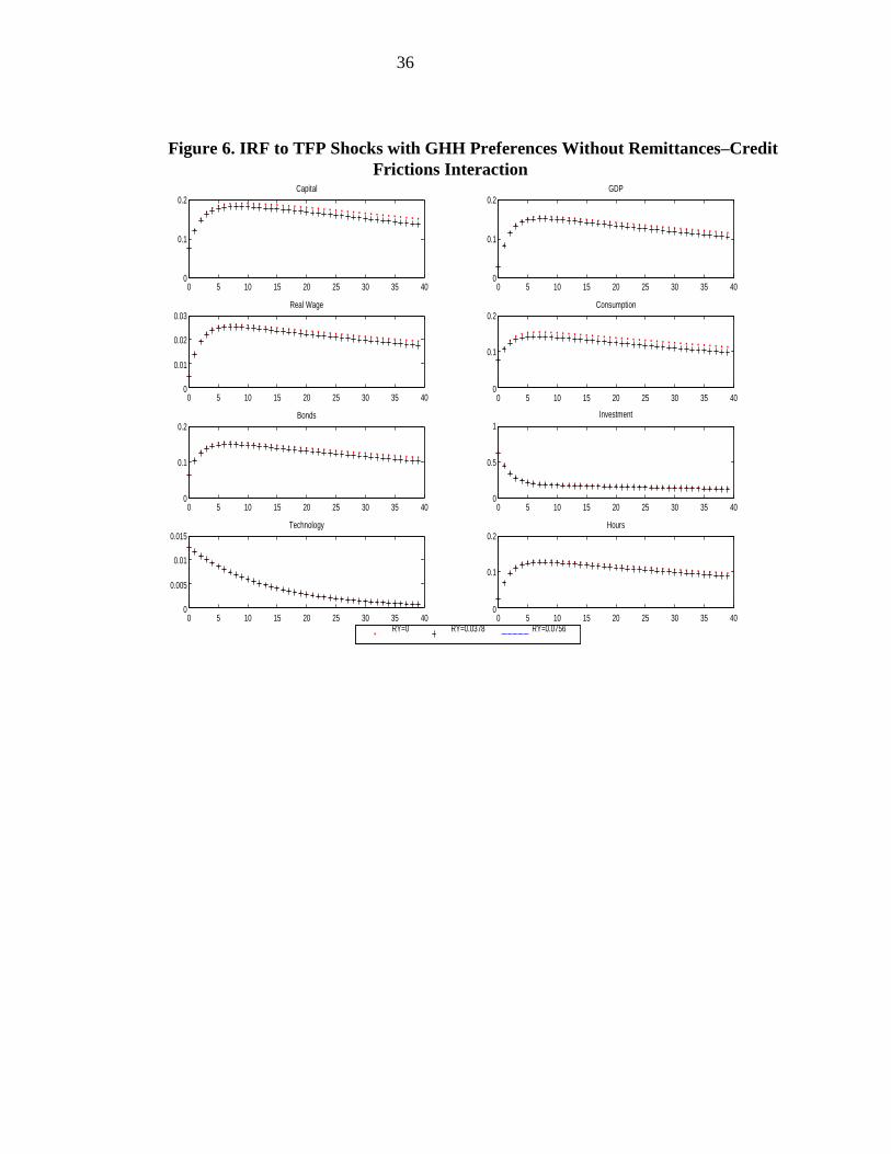
36

Figure 6. IRF to TFP Shocks with GHH Preferences Without Remittances–Credit

Frictions Interaction

0.2

Capital 0.2

GDP

0.1 0.1

0

0.03

0 5 10 15 20 25 30 35 40

Real Wage

0

0.2

0 5 10 15 20 25 30 35 40

Consumption

0.02

0.01

0.1

0

0.2

0 5 10 15 20 25 30 35 40

Bonds

0

0 5 10 15 20 25 30 35 40

Investment

1

0.1 0.5

0

0.015

0 5 10 15 20 25 30 35 40

Technology

0

0.2

0 5 10 15 20 25 30 35 40

Hours

0.01

0.005

0.1

0

0 5 10 15 20 25 30 35 40

0

0 5 10 15 20 25 30 35 40 RY=0 RY=0.0378 RY=0.0756

37

Figure 7. IRF to TFP shocks with GHH Preferences and Remittances–Credit Frictions

Interaction

0.2

Capital 0.2

GDP

0.1 0.1

0

0.03

0 5 10 15 20 25 30 35 40

Real Wage

0

0.2

0 5 10 15 20 25 30 35 40

Consumption

0.02

0.01

0.1

0

0.2

0 5 10 15 20 25 30 35 40

Bonds

0

0 5 10 15 20 25 30 35 40

Investment

1

0.1 0.5

0

0.015

0 5 10 15 20 25 30 35 40

Technology

0

0.2

0 5 10 15 20 25 30 35 40

Hours

0.01

0.005

0.1

0

0 5 10 15 20 25 30 35 40

0

0 5 10 15 20 25 30 35 40 RY=0 RY=0.0378 RY=0.0756