Embed Size (px)
Citation preview
Int. Journal of Economics and Management 8(1): 10 – 39 (2014) ISSN 1823 - 836X
Macroeconomic Fundamentals and Exchange Rate Volatility during the Floating Exchange
Rate Regime in India
ANup KuMAr SAhAa ANd SrEElAtA BISwASb*a,bDepartment of Economics, Nabadwip Vidyasagar College, West-Bengal,
B-3/64, Kalyani , Dist- Nadia, Pin-741235,West-Bengal, India
ABSTRACTExchange rate stability is one of the pre-conditions for macro-economic stability. So choice of exchange rate regime is the core of the successful macro-management. India has opted market-determined exchange rate system since 1993. Exchange rate volatility arises due to macro-economic fundamentals like growth, trade, price level, interest rate, foreign exchange reserve etc. and short-term speculation. we have estimated the relationship between exchange rate and the fundamental macro-variables using the Vector Error Correction Model (VECM) with monthly data for the period April, 1993 to March, 2012. It is found that export, interest rate, foreign exchange reserve and economic growth have appreciating effect where as import and inflation have depreciating effect on exchange rate. All the variables under the study other than interest rate and the foreign exchange reserve have played significant role in exchange rate stabilization during the floating exchange rate regime. In the short-run, exchange rate is negatively influenced by its own lags and interest rate as well as foreign exchange reserve. But it is positively affected by country’s import. Generalized variance decompositions indicate that interest rate, economic growth and inflation have stronger impact on exchange rate.
Keywords: foreign exchange policy, open economy macro economies, volatility, VECM, India.
JEL classification: O24, F41, E32, C22, O53.
* Corresponding Author: E-mail: [email protected], [email protected] remaining errors or omissions rest solely with the author(s) of this paper.
11
Macroeconomic Fundamentals and Exchange Rate Volatility
INTRODUCTIONExchange rate is one of the important key policy variables for better macroeconomic management. Macroeconomic stability in the external front largely depends on the proper choice of exchange rate regime. It is the exchange rate volatility which affects directly the international trade and thereby the growth and domestic price level. Movements in exchange rates are a natural feature of countries’ adjustment over the business cycle. The cyclical behavior of exchange rates reflects changes in monetary policy over the business cycle, and thus it provides one of the channels through which short-run stabilization policy operates. So a country’s economic health depends considerably on the appropriate choice of the exchange rate regime.
the importance of exchange rate as an immediate tool of macro management reached its highest point at the onset of the new economic reform during the early years of 1990 in India. It further gained attention from the policy-makers during the East Asian currency crisis. Substantial intervention by the reserve Bank of India (rBI) in both spot and forward exchange markets to curb excessive volatility saved India from the spillover of East Asian contagion in 1998. India has opted for a market-determined exchange rate system since early 1993. we are concerned with the volatility of the exchange rate during the floating exchange rate period. Volatility of the exchange rate in case of market determined system can arise due to following two factors:
1. Volatility due to the macro-economic fundamentals that is economic growth, volume of trade, inflation, interest rate differential etc. and
2. Volatility due to short-term speculative phenomena and changes in investor’s sentiment and expectation.
We have rationally assumed that the second factor acts as an automatic stabilizer in the currency market. So we are basically interested here with the exchange rate volatility in relation to some important macro-economic variables. the present paper is divided into six sections. The first section provides an overview of the different exchange rate regimes in general. Section two describes different exchange rate regimes. Section three deals with the evolution and structural changes of exchange rate regime in India. Section four illustrates the exchange rate volatility. Section five describes the relation between exchange rate and other important macro variables. data range and variables are described in Section six. Entire methodology and the empirical analysis are provided in Section seven. Finally Section eight concludes the paper.
12
International Journal of Economics and Management
AN OVERVIEw OF ThE ExChANgE RATE REgIMESExchange rate regime is the mechanism, procedures and institutional arrangement for determining exchange rates at a point of time and changes in them over time. theoretically a large number of exchange rate regimes are possible. According to IMF (2001), the exchange rate regime can be broadly classified in to eight categories: (1) exchange arrangements with no separate legal tender, (2) currency board arrangements, (3) other conventional fixed peg arrangements, (4) pegged exchange rates within horizontal bands, (5) crawling pegs, (6) exchange rates within crawling bands, (7) managed floating with no preannounced path for the exchange rate and (8) independently floating.
there are two extremes in exchange rate management mechanism. perfectly rigid or hard peg or fixed is in one extreme and perfectly floating or flexible exchange rate is in another extreme. In between two there is large number of exchange rate regimes, having different degree of mix of both the extreme regimes. Basically exchange rate regime followed by a nation determines its parity with respect to a particular foreign currency like uS dollar, pound, Euro etc. or a basket of foreign currencies.
Government intervenes in order to maintain the exchange rate at a certain prescribed level or within a range in case of fixed exchange rate regime. Central monetary authority keeps on buying and selling in the foreign exchange market to curtail the variability of the exchange rate. As a result of this, monetary authority loses its control over the money supply. So it is very much customary to expect that the fixed exchange rate regime with perfect capital mobility can raise serious problem of inflation or price volatility.
There are mainly two variants of the fixed exchange rate regime, namely the crawling peg and the adjustable peg regimes. In the case of the crawling peg, the government makes frequent but small adjustments to the pegged rate while in the case of the adjustable peg, the adjustments are infrequent. Crawling peg or adjustable peg permits the monetary authority to keep lesser amount of foreign exchange reserve than the fixed exchange rate regime as a buffer to finance balance of payments deficit because of greater reliance on the exchange rate changes. however, if future exchange rate movements are not predetermined, speculation of exchange rate changes based on inflationary expectations might arise and this could generate instability.
On the other extreme, a freely flexible exchange rate regime exists when exchange rates are freely determined by market forces, i.e. by the demand for and supply of currencies by private agents. Monetary authorities do not have to involve with balance of payments problems as they are under no obligation to intervene in
13
Macroeconomic Fundamentals and Exchange Rate Volatility
the foreign exchange market. thus they need not be concerned actively with the movement of the international reserve and so they can exercise more effective role over the domestic money supply. A variant of the flexible exchange rate regime is the managed float regime. It involves government intervention in the foreign exchange market in order to control the exchange rate movement though it involves no commitment to maintain a certain fixed rate or some narrow band around it.
world had experienced several types of exchange rate regimes during the last century. But grossly they can be classified into three categories on the basis of their worldwide acceptance as a policy of external stability. these are classical period of the gold standard (1870-1914), fixed exchange rate regime (1944-1971) and flexible exchange rate regime. The first modern international monetary system was the gold standard. Operating during the late 19th and early 20th centuries, the gold standard provided for the free circulation between nations of gold coins of standard specification. Under the system, gold was the only standard of value. during the 1920s the gold standard was replaced by the gold bullion standard, under which nations no longer minted gold coins but backed their currencies with gold bullion and agreed to buy and sell the bullion at a fixed price. This system, too, was abandoned in the 1930s. Finally, the Gold Exchange Standard came into force, which was defined by Encyclopedia Britannica as the monetary system under which a nation’s currency may be converted into bills of exchange drawn on a country whose currency is convertible into gold at a stable rate of exchange. A nation on the gold-exchange standard is thus able to keep its currency at parity with gold without having to maintain as large a gold reserve as is required under the gold standard.
In the classical period of the gold standard, external disturbance of the economy is overcome causing internal disturbance. Deficits in the external front were to be adjusted by internal deflation, and surpluses were to be removed by internal inflation. the international monetary system, during this period of gold standard, can therefore be described as one of fixed exchange rates. The system worked moderately well as no major currency crisis or financial crisis did not occur during that time across the globe. Fairly stable exchange rates remained across the nations. International trade and finance flourished during that time. But it did not perform well with the deficit country. Huge unemployment pressure resulting in recession engulfed a large number of nations. this situation continued till world war I. world war I was a turning point. the gold standard was abandoned. Attempts to revive the gold standard were in vein. the inter-war period was a very chaotic one. It could not be described under a single umbrella. during that time exchange rate volatility increased. But the period could not be described as a period of flexible exchange rate regime. Sterling lost its status as international currency.
14
International Journal of Economics and Management
Then the period of fixed exchange rate system commonly known as the Bretton woods system came into action from 1944. In that system, a country changed its exchange rate only when it required correcting a fundamental disequilibrium in BOp situation of a country. the system collapsed in 1971 following the dollar crisis. dollar crisis led to the Smithsonian Agreement of december 1971. under that agreement currency realignment was recommended. As a result of this devaluation of uS dollar, revaluation of most European currencies and of the Japanese Yen took place. Smithsonian Agreement failed within a short span of time and the uS dollar was devalued again. therefore, the period from 1971 to 1976 can be considered as one of informal flexible exchange rates. The Jamaica Agreement of January 1976 formalized flexible exchange rates, which had come into practice by then anyway. Since 1976, flexible exchange rate is followed.
In the flexible exchange rate regime, exchange rate is determined by the market forces resulting into significant amount of short-run volatility and occasional large medium-run swings. Macroeconomic imbalances like current account disturbance in this system are overcome largely by the international private capital flow. International agencies mainly International Monetary Fund comes forward in case of severe disturbance. International financial disturbances pass through this flexible exchange rate channel very easily within a very short span of time. developed industrial countries along with a significant number of emerging economies have already abandoned the fixed exchange rate regime and moved towards a market determined flexible exchange rate regime.
EVOlUTION AND STRUCTURAl ChANgES OF ExChANgE RATE REgIME (DE jURE) IN INDIA
Indian national currency that is rupee had been linked with the pound Sterling from the pre-independence period and it continued until mid-december 1973 except for some contingent situations like devaluations in 1966 and 1971. rupee discontinued its link with the pound Sterling from 1976 onwards and since then India followed a managed floating exchange rate regime till 1990. It maintained its exchange rate parity with a “basket of currencies” comprising the major currencies of the nations with which it had significant level of trade relation. During early nineties India faced a severe balance of payment crisis due to increase in trade deficit and net invisible deficit. Downward adjustment of Rupee took place in two stages. Liberalized Exchange rate Management System (lErMS) was introduced in March 1992. Following this management system India stepped into dual exchange rate regime that is official as well as market determined exchange rate system till 1993.
15
Macroeconomic Fundamentals and Exchange Rate Volatility
All the foreign exchange remittances into India earned through export of goods or services or through inward remittances were allowed to be converted into two following manners:
1. Sixty per cent of the total earnings can be converted into domestic currency by market determined rate and this proceeding can be used for the transaction in current account.
2. remaining forty per cent remained under the supervision of the central bank. It should be sold to the RBI through authorized dealers at the official rate of exchange. rBI used this amount to facilitate the preferred or contingent amount of import of the government. It was observed that market determined exchange rate always remained higher than the official exchange rate as it was expected. Basically this gap was the motivating force behind the black marketing of the exchange rate during that time. Nevertheless, dual exchange rate regime has achieved its goal to ease the balance of payment situation. Foreign exchange reserve multiplied by five times between 1990-91 and 1994-95.
But the surrender of forty per cent earnings of the exporters at the official exchange rate made a major bleeding to the exporters. therefore to boost up the export sector India had to move towards a fully market determined exchange rate regime. Currency was made fully convertible under the trade account and subsequently it also made fully convertible under the current account transaction. however rBI was empowered to intervene in the foreign exchange market to moderate the exchange rate volatility whenever large swing is observed in the market. India is preparing a roadmap to make its currency fully convertible even under the capital account.
ExChANgE RATE VOlATIlITy
Measure of VolatilityOne of the most common measures of exchange rate volatility is the standard deviation of the growth rates of real exchange rates (V). this measure is approximated by a time-varying measure defined as follows:
V r R R1t r t i t ii
r1 2
21
1 2
= -+ + - + -= ^ h9 C/
where R is the natural log of the bilateral real exchange rate/real effective exchange rate and r is the order of the moving average. the order of the present study is 12 as we have used monthly data.
16
International Journal of Economics and Management
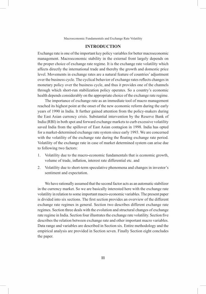
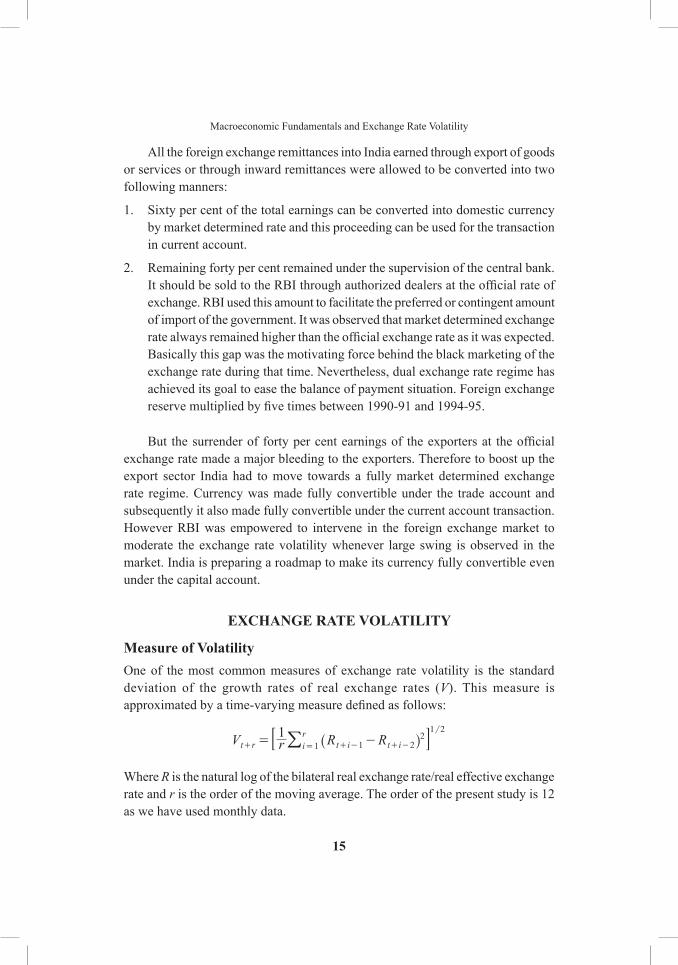
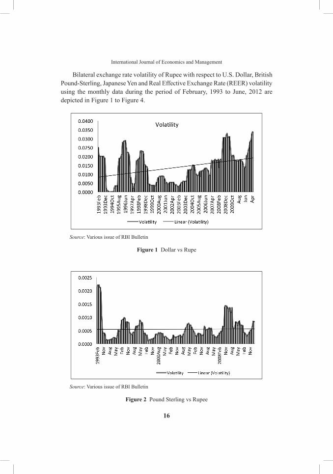
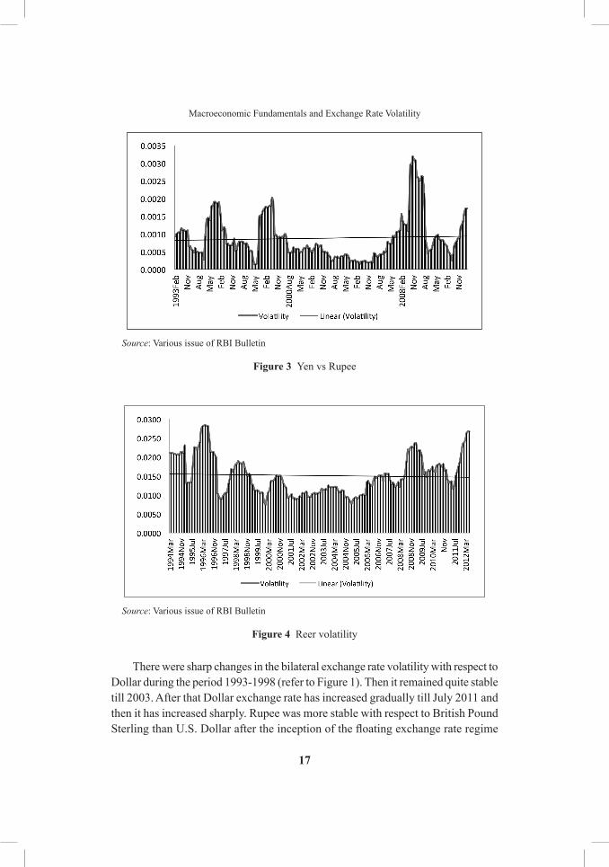
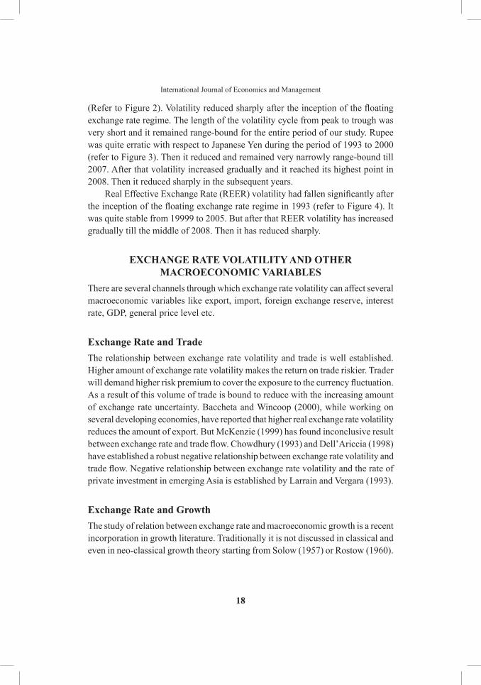
Bilateral exchange rate volatility of rupee with respect to u.S. dollar, British pound-Sterling, Japanese Yen and real Effective Exchange rate (rEEr) volatility using the monthly data during the period of February, 1993 to June, 2012 are depicted in Figure 1 to Figure 4.
Source: Various issue of rBI Bulletin
Figure 1 dollar vs rupe
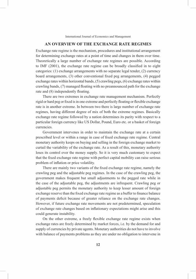
Source: Various issue of rBI Bulletin
Figure 2 pound Sterling vs rupee
17
Macroeconomic Fundamentals and Exchange Rate Volatility
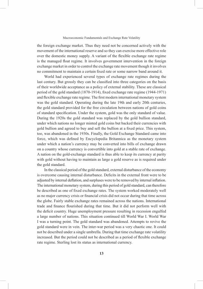
Source: Various issue of rBI Bulletin
Figure 3 Yen vs rupee
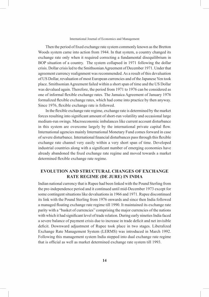
Source: Various issue of rBI Bulletin
Figure 4 reer volatility
there were sharp changes in the bilateral exchange rate volatility with respect to dollar during the period 1993-1998 (refer to Figure 1). then it remained quite stable till 2003. After that dollar exchange rate has increased gradually till July 2011 and then it has increased sharply. rupee was more stable with respect to British pound Sterling than U.S. Dollar after the inception of the floating exchange rate regime
18
International Journal of Economics and Management
(Refer to Figure 2). Volatility reduced sharply after the inception of the floating exchange rate regime. the length of the volatility cycle from peak to trough was very short and it remained range-bound for the entire period of our study. rupee was quite erratic with respect to Japanese Yen during the period of 1993 to 2000 (refer to Figure 3). then it reduced and remained very narrowly range-bound till 2007. After that volatility increased gradually and it reached its highest point in 2008. then it reduced sharply in the subsequent years.
Real Effective Exchange Rate (REER) volatility had fallen significantly after the inception of the floating exchange rate regime in 1993 (refer to Figure 4). It was quite stable from 19999 to 2005. But after that rEEr volatility has increased gradually till the middle of 2008. then it has reduced sharply.
ExChANgE RATE VOlATIlITy AND OThER MACROECONOMIC VARIABlES
there are several channels through which exchange rate volatility can affect several macroeconomic variables like export, import, foreign exchange reserve, interest rate, Gdp, general price level etc.
Exchange Rate and Tradethe relationship between exchange rate volatility and trade is well established. higher amount of exchange rate volatility makes the return on trade riskier. trader will demand higher risk premium to cover the exposure to the currency fluctuation. As a result of this volume of trade is bound to reduce with the increasing amount of exchange rate uncertainty. Baccheta and wincoop (2000), while working on several developing economies, have reported that higher real exchange rate volatility reduces the amount of export. But McKenzie (1999) has found inconclusive result between exchange rate and trade flow. Chowdhury (1993) and Dell’Ariccia (1998) have established a robust negative relationship between exchange rate volatility and trade flow. Negative relationship between exchange rate volatility and the rate of private investment in emerging Asia is established by larrain and Vergara (1993).
Exchange Rate and growththe study of relation between exchange rate and macroeconomic growth is a recent incorporation in growth literature. traditionally it is not discussed in classical and even in neo-classical growth theory starting from Solow (1957) or rostow (1960).
19
Macroeconomic Fundamentals and Exchange Rate Volatility
Even in the endogenous growth theory the impact of exchange rate dynamics on overall economic growth is not addressed. rodrick (2008) has provided evidence that undervaluation of the currency (a high real ex-change rate) stimulates economic growth particularly in some developing countries including India. the positive impact of exchange rate stability on growth is particularly strong for Emerging Europe, i.e., the central, eastern and south-eastern European countries, and the countries which belong to the Commonwealth of Independent States. For the industrialized non-EMU countries where capital markets are more developed the negative impact of exchange rate volatility on growth is less pronounced. the non-European countries which border the Mediterranean Sea do not show a significant impact of exchange rate stability on growth. this could be due to the fact that in this region the exchange rate pegs are often supported by tight capital account and interest rate controls (Schnable, 2007).
the interrelationship between exchange rate and growth is better understood with the help of the export-led growth hypothesis. Following this hypothesis, government, especially in the comparatively closed economies, can provide the impetus to the export oriented sector using the real exchange rate in favor of exportable sector relative to the non-tradable sector. As a result of this production of the manufacturing sector, the most important export-oriented sector, increases due to the greater amount of resource mobilization in the sector. Higher productivity in manufacturing than in agriculture provides higher amount of income growth consistently without encountering diminishing returns like those experienced in agricultural sector. It can continue without driving down prices insofar as external demand is elastic, unlike the situation with non-tradable, where demand is purely domestic and therefore relatively inelastic. It thus allows the structure of production to be disconnected from the structure of consumption. If higher incomes and faster growth support higher savings, then it will become possible to finance higher levels of investment out of domestic resources. If learning-by-doing or technology transfer is relatively rapid in sectors producing for export, then there will be additional stimulus to the overall rate of growth. That first Japan, then Hong Kong, Singapore, South Korea and taiwan, and now China have had success with this model has directed attention to the real exchange rate as a development-relevant policy tool. Indeed, it is hard to think of many developing countries that have sustained growth accelerations in the presence of an overvalued rate. the Bretton woods II model of the world economy is essentially a story about the external consequences of the adoption of a competitive real exchange rate as a growth strategy by developing countries (Eichengreen, 2008).
20
International Journal of Economics and Management
Exchange Rate and Interest Ratethe empirical literature on the nexus between interest rate and exchange rate is inconclusive. theoretically the relationship between exchange rate and interest rate can be established with the help of the following channels. First, higher domestic interest rates raise the demand for the deposits, and, hence, the money base. Second, firms need bank loans to finance the production process, so higher interest rate makes the borrowing costly and thereby makes the cost of production higher. As a result of this the amount of production reduces. Supply shortage further increases the inflationary pressure within the economy. Lastly, higher interest rates raise the government’s fiscal burden which is again inflationary in nature. While the first effect tends to appreciate the currency, the remaining two effects tend to depreciate it. however reduction of exchange rate volatility may come at the cost of higher interest rate variability, which in turn may translate into higher variability on debt servicing costs for developing countries (reinhart and reinhart, 2003). high interest rate (presumably, real) , results in larger country risk premia – so much so, that the expected return to the investors actually declines as interest rates increase, thus prompting even greater capital flight, and generating more downward pressure on the exchange rate (Basurto and Ghosh, 2000). Empirical evidences from the emerging economies indicate that raising nominal interest rates leads to a higher probability of switching to the crisis regime (Neumeyer and perri, 2005). So higher interest rate policy has failed to tame the exchange rate variability in those nations.
Exchange Rate and Inflationthe predominant view on the relationship between the exchange rate regime and inflation is that pegged exchange rates contribute to lower and more stable inflation. For developing and emerging countries with comparatively weak institutional frameworks, pegged exchange rates provide an important tool to control inflation via both a commitment toward exchange rate stability and a disciplining effect on monetary growth (Crockett and Goldstein, 1976). For small, open economies, pegging the nominal exchange rate helps minimize fluctuations of the domestic price level and thereby contributes to macroeconomic stability (McKinnon, 1963).
In contrast, in countries with strong institutional frameworks (based on central bank independence and developed money markets), low inflation can be achieved without any specific commitment to an explicit exchange rate target (Calvo and Mishkin, 2003). Recently, inflation-targeting frameworks have become a widely used tool to achieve price stability in both industrial countries and emerging markets.
21
Macroeconomic Fundamentals and Exchange Rate Volatility
Exchange Rate and Foreign Exchange Reservetheoretically exchange rate stability has a positive association with the foreign exchange reserve of a nation because of favorable trade balance. however, increase in foreign exchange reserves increases the monetary base of the economy. As a result of this domestic currency appreciates and thereby reduces the export earning of the economy.
the present study aims to examine empirically the relationships between exchange rate (real Effective Exchange rate) and six other related macro variables viz. export, import, interest rate, inflation, foreign exchange reserve and GDP growth rate. we have tried to establish the dynamic interaction between exchange rate and other variables using Vector Error Correction Model (VECM), Variance decomposition Analysis and Impulse response Function. the macro variables are chosen on the basis of standard macro and trade theory and supported or justified with the previous empirical established literature. Our approach is different from the previous approaches because of its broad-based nature including all the related variables.
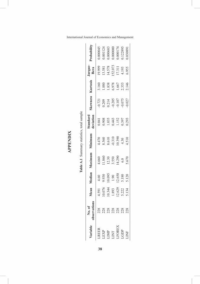
DATA AND METhODOlOgywe have used monthly time series to get the long run relationship between rEEr and the other related macro variables. the sample period is April, 1993 to March, 2012. the secondary data source is the hand book of Statistics, 2011-12, rBI. All the variables are transformed into their natural logarithmic form to reduce the fluctuation in the data set. The summary statistics of the data is provided in the Appendix (See Table A.1 in the Appendix) the following functional form between rEEr and other related macro variables is assumed as follows:
LREERt = β0 + β1 LEXPt + β2 LIMPt + β3 LINTt + β4 LFOREXt + β5 LINFt + β6 LGDPt + ∈t (1)
where:β0 = constant or intercept term.t = deterministic trend.∈ = the stochastic error term.lrEEr = home country exchange rate as measured by the natural logarithm
of the monthly real effective exchange rate index (using trade-based weights, base: 1993-94) of India. In fact, rEEr is weighted
22
International Journal of Economics and Management
average (36- country) of the bilateral nominal exchange rates of the home country’s currency relative to an index or basket of other major foreign currencies adjusted for the effects of inflation. The interpretation of rEEr is that if the index increases, the purchasing power of home currency is higher against those of the country’s trading partners. Conversely a lower index means that the home currency depreciated.
lEXp = natural logarithm of export volume.lIMp = natural logarithm of Import volume.lINt = natural logarithm of interest rate. Call Money rate is used here as
a proxy of interest rate.lFOrEX = natural logarithm of foreign exchange reserve.LINF = natural logarithm of inflation. Monthly data of WPI is used as a
proxy for inflation.lGdp = natural logarithm of Gdp. As monthly data of Gdp is not available,
we used monthly data of Index of Industrial production (IIp) as a proxy of Gdp data.
The βs are the coefficients to be estimated. The expected signs for β1, β4, β6 are positive, that of β2 and β5 are negative and β3 may be positive or negative.
EMpIRICAl ANAlySIS
Stationarity Teststhe classical regression model requires that the dependent and independent variables in a regression be stationary in order to avoid the problem of what Granger and Newbold (1974) called ‘spurious regression’. Nonstationarity can be tested using the Augmented dickey-Fuller (AdF) test, the phillips perron (pp) test and the Kwiatkowski-phillips-Schmidt-Shin (KpSS) test.
ADF Testthe test is conducted with the following set of regression equations
Y Y i Yt t t i ti
p
1 11
T T !b i c= + + +- -=
/ (2)
tY t Y i Yt t t ii
p
1 2 11
dT Tb b i c= + + + +- -=
/ (3)
23
Macroeconomic Fundamentals and Exchange Rate Volatility
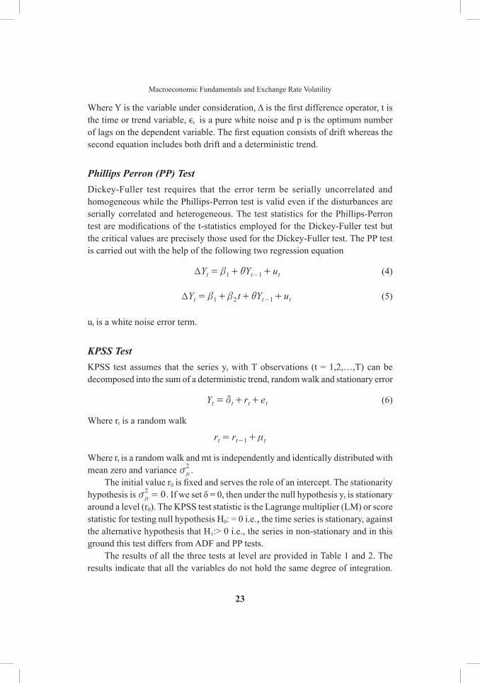
Where Y is the variable under consideration, Δ is the first difference operator, t is the time or trend variable, ϵt is a pure white noise and p is the optimum number of lags on the dependent variable. The first equation consists of drift whereas the second equation includes both drift and a deterministic trend.
Phillips Perron (PP) Testdickey-Fuller test requires that the error term be serially uncorrelated and homogeneous while the phillips-perron test is valid even if the disturbances are serially correlated and heterogeneous. the test statistics for the phillips-perron test are modifications of the t-statistics employed for the Dickey-Fuller test but the critical values are precisely those used for the dickey-Fuller test. the pp test is carried out with the help of the following two regression equation
Y Y ut t t1 1T b i= + +- (4)
Y t Y ut t t1 2 1T b b i= + + +- (5)
ut is a white noise error term.
KPSS TestKpSS test assumes that the series yt with t observations (t = 1,2,…,t) can be decomposed into the sum of a deterministic trend, random walk and stationary error
Y r et t t td= + + (6)
where rt is a random walk
r rt t t1 n= +-
where rt is a random walk and mt is independently and identically distributed with mean zero and variance 2vn .
the initial value r0 is fixed and serves the role of an intercept. The stationarity hypothesis is 02v =n . If we set δ = 0, then under the null hypothesis yt is stationary around a level (r0). the KpSS test statistic is the lagrange multiplier (lM) or score statistic for testing null hypothesis h0: = 0 i.e., the time series is stationary, against the alternative hypothesis that h1:> 0 i.e., the series in non-stationary and in this ground this test differs from AdF and pp tests.
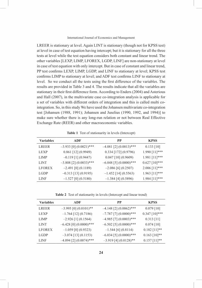
the results of all the three tests at level are provided in table 1 and 2. the results indicate that all the variables do not hold the same degree of integration.
24
International Journal of Economics and Management
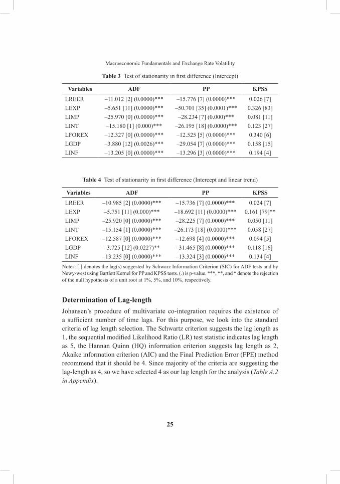
lrEEr is stationary at level. Again lINt is stationary (though not for KpSS test) at level in case of test equation having intercept; but it is stationary for all the three tests at level while the test equation considers both constant and linear trend. the other variables [lEXp, lIMp, lFOrEX, lGdp, lINF] are non-stationary at level in case of test equation with only intercept. But in case of constant and linear trend, PP test confirms LEXP, LIMP, LGDP, and LINF to stationary at level; KPSS test confirms LIMP to stationary at level; and ADF test confirms LINF to stationary at level. So we conduct all the tests using the first difference of the variables. The results are provided in table 3 and 4. the results indicate that all the variables are stationary in their first difference form. According to Enders (2004) and Asterious and hall (2007), in the multivariate case co-integration analysis is applicable for a set of variables with different orders of integration and this is called multi co-integration. So, in this study we have used the Johansen multivariate co-integration test [Johansen (1988, 1991); Johansen and Juselius (1990, 1992, and 1994)] to make sure whether there is any long-run relation or not between real Effective Exchange rate (rEEr) and other macroeconomic variables.
Table 1 test of stationarity in levels (Intercept)
Variables ADF pp KpSS
lrEEr –3.933 [0] (0.0021)*** –4.081 [2] (0.0013)*** 0.133 [10] lEXp 0.861 [12] (0.9949) 0.334 [172] (0.9796) 1.990 [11]***lIMp –0.119 [1] (0.9447) 0.047 [10] (0.9609) 1.981 [11]***lINt –3.808 [2] (0.0033)*** –6.048 [5] (0.0000)*** 0.627 [10]***lFOrEX –2.491 [0] (0.1189) –2.086 [6] (0.2507) 2.006 [11]***lGdp –0.313 [13] (0.9195) –1.452 [14] (0.5563) 1.963 [11]***lINF –1.527 [0] (0.5180) –1.384 [4] (0.5896) 1.984 [11]***
Table 2 test of stationarity in levels (Intercept and linear trend)
Variables ADF pp KpSS
lrEEr –3.995 [0] (0.0101)** –4.148 [2] (0.0062)*** 0.079 [10]lEXp –1.764 [12] (0.7186) –7.787 [7] (0.0000)*** 0.347 [10]***lIMp –2.926 [1] (0.1564) –4.985 [7] (0.0003)*** 0.313 [11]lINt –6.428 [0] (0.0000)*** –6.502 [5] (0.0000)*** 0.074 [10]lFOrEX –1.059 [0] (0.9323) –1.544 [6] (0.8114) 0.182 [11]**lGdp –3.074 [13] (0.1153) –6.034 [5] (0.0000)*** 0.163 [10]**lINF –4.094 [2] (0.0074)*** –3.919 [4] (0.0128)** 0.157 [11]**
25
Macroeconomic Fundamentals and Exchange Rate Volatility
Table 3 Test of stationarity in first difference (Intercept)
Variables ADF pp KpSS
lrEEr –11.012 [2] (0.0000)*** –15.776 [7] (0.0000)*** 0.026 [7]lEXp –5.651 [11] (0.0000)*** –50.701 [35] (0.0001)*** 0.326 [83]lIMp –25.970 [0] (0.0000)*** –28.234 [7] (0.000)*** 0.081 [11]lINt –15.180 [1] (0.000)*** –26.195 [18] (0.0000)*** 0.123 [27]lFOrEX –12.327 [0] (0.0000)*** –12.525 [5] (0.0000)*** 0.340 [6]lGdp –3.880 [12] (0.0026)*** –29.054 [7] (0.0000)*** 0.158 [15]lINF –13.205 [0] (0.0000)*** –13.296 [3] (0.0000)*** 0.194 [4]
Table 4 Test of stationarity in first difference (Intercept and linear trend)
Variables ADF pp KpSS
lrEEr –10.985 [2] (0.0000)*** –15.736 [7] (0.0000)*** 0.024 [7]lEXp –5.751 [11] (0.000)*** –18.692 [11] (0.0000)*** 0.161 [79]**lIMp –25.920 [0] (0.0000)*** –28.225 [7] (0.0000)*** 0.050 [11]lINt –15.154 [1] (0.0000)*** –26.173 [18] (0.0000)*** 0.058 [27]lFOrEX –12.587 [0] (0.0000)*** –12.698 [4] (0.0000)*** 0.094 [5]lGdp –3.725 [12] (0.0227)** –31.465 [8] (0.0000)*** 0.118 [16]lINF –13.235 [0] (0.0000)*** –13.324 [3] (0.0000)*** 0.134 [4]
Notes: [.] denotes the lag(s) suggested by Schwarz Information Criterion (SIC) for ADF tests and by Newy-west using Bartlett Kernel for pp and KpSS tests. (.) is p-value. ***, **, and * denote the rejection of the null hypothesis of a unit root at 1%, 5%, and 10%, respectively.
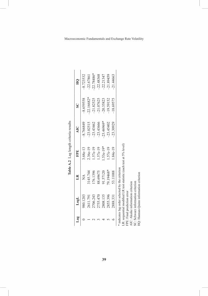
Determination of lag-lengthJohansen’s procedure of multivariate co-integration requires the existence of a sufficient number of time lags. For this purpose, we look into the standard criteria of lag length selection. The Schwartz criterion suggests the lag length as 1, the sequential modified Likelihood Ratio (LR) test statistic indicates lag length as 5, the hannan Quinn (hQ) information criterion suggests lag length as 2, Akaike information criterion (AIC) and the Final prediction Error (FpE) method recommend that it should be 4. Since majority of the criteria are suggesting the lag-length as 4, so we have selected 4 as our lag length for the analysis (Table A.2 in Appendix).
26
International Journal of Economics and Management
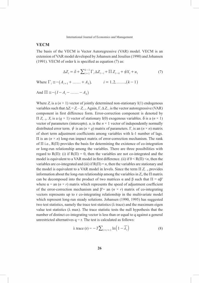
VECMthe basis of the VECM is Vector Autoregressive (VAr) model. VECM is an extension of VAr model developed by Johansen and Jesulius (1990) and Johansen (1991). VECM of order k is specified as equation (7) as:
Z Z Z X ut i t ii
kt k t t1
1T Td }C P= + + + +-=
--/ (7)
where ,, , ,A A ki 11 2i i k1 ff ff/C - + + -=+^ ^h h
And I A Ai kff/P - - - -^ h
where Zt is a (n × 1) vector of jointly determined non-stationary I(1) endogenous variables such that ∆Zt = Zt – Zt–1. Again, Γi Δ Zt–i is the vector autoregressive (VAr) component in first difference form. Error-correction component is denoted by Π Zt – k. Xt is a (q × 1) vector of stationary I(0) exogenous variables. δ is a (n × 1) vector of parameters (intercepts). ut is the n × 1 vector of independently normally distributed error term. } is an (n × q) matrix of parameters. Γi is an (n × n) matrix of short term adjustment coefficients among variables with k-1 number of lags. Π is an (n × n) long-run impact matrix of error-correction mechanism. the rank of Π i.e., R(Π) provides the basis for determining the existence of co-integration or long-run relationship among the variables. there are three possibilities with regard to R(Π): (i) if R(Π) = 0, then the variables are not co-integrated and the model is equivalent to a VAR model in first difference. (ii) if 0 < R(Π) <n, then the variables are co-integrated and (iii) if R(Π) = n, then the variables are stationary and the model is equivalent to a VAR model in levels. Since the term Π Zt – k provides information about the long-run relationship among the variables in Zt, the Π matrix can be decomposed into the product of two matrices α and β such that Π = αβ′ where α = an (n × r) matrix which represents the speed of adjustment coefficient of the error-correction mechanism and β′= an (n × r) matrix of co-integrating vectors represents up to r co-integrating relationship in the multivariate model which represent long-run steady solutions. Johansen (1990, 1995) has suggested two test statistics, namely the trace test statistics (λ trace) and the maximum eigen value test statistics (λ max). The trace statistic tests the null hypothesis that the number of distinct co-integrating vector is less than or equal to q against a general unrestricted alternatives q = r. the test is calculated as follows:
λ trace (r) = lnT 1 ti r 1 m- -= +a kX/ (8)
27
Macroeconomic Fundamentals and Exchange Rate Volatility
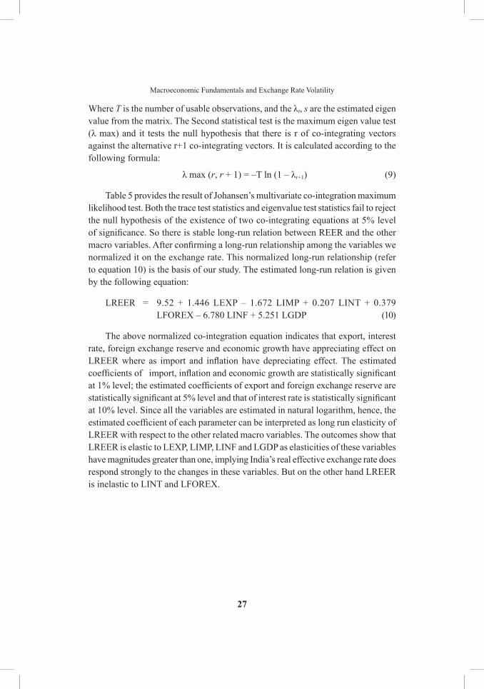
where T is the number of usable observations, and the λt, s are the estimated eigen value from the matrix. the Second statistical test is the maximum eigen value test (λ max) and it tests the null hypothesis that there is r of co-integrating vectors against the alternative r+1 co-integrating vectors. It is calculated according to the following formula:
λ max (r, r + 1) = –T ln (1 – λr+1) (9)
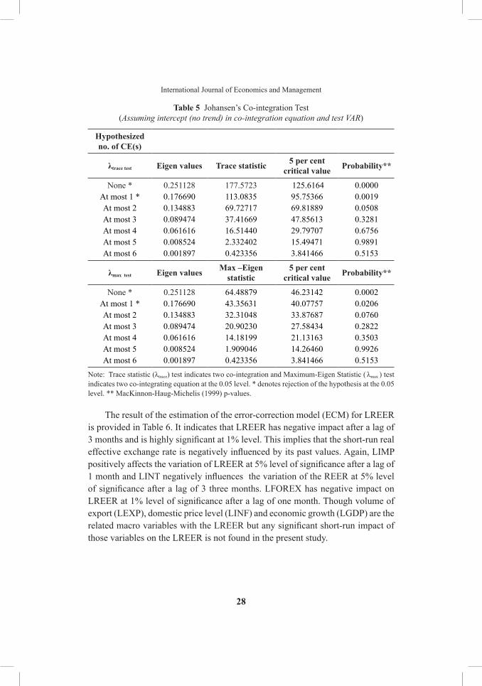
table 5 provides the result of Johansen’s multivariate co-integration maximum likelihood test. Both the trace test statistics and eigenvalue test statistics fail to reject the null hypothesis of the existence of two co-integrating equations at 5% level of significance. So there is stable long-run relation between REER and the other macro variables. After confirming a long-run relationship among the variables we normalized it on the exchange rate. This normalized long-run relationship (refer to equation 10) is the basis of our study. the estimated long-run relation is given by the following equation:
lrEEr = 9.52 + 1.446 lEXp – 1.672 lIMp + 0.207 lINt + 0.379 lFOrEX – 6.780 lINF + 5.251 lGdp (10)
The above normalized co-integration equation indicates that export, interest rate, foreign exchange reserve and economic growth have appreciating effect on LREER where as import and inflation have depreciating effect. The estimated coefficients of import, inflation and economic growth are statistically significant at 1% level; the estimated coefficients of export and foreign exchange reserve are statistically significant at 5% level and that of interest rate is statistically significant at 10% level. Since all the variables are estimated in natural logarithm, hence, the estimated coefficient of each parameter can be interpreted as long run elasticity of lrEEr with respect to the other related macro variables. the outcomes show that lrEEr is elastic to lEXp, lIMp, lINF and lGdp as elasticities of these variables have magnitudes greater than one, implying India’s real effective exchange rate does respond strongly to the changes in these variables. But on the other hand lrEEr is inelastic to lINt and lFOrEX.
28
International Journal of Economics and Management
Table 5 Johansen’s Co-integration test (Assuming intercept (no trend) in co-integration equation and test VAR)
hypothesized no. of CE(s)
λtrace test Eigen values Trace statistic 5 per cent critical value probability**
None * 0.251128 177.5723 125.6164 0.0000At most 1 * 0.176690 113.0835 95.75366 0.0019At most 2 0.134883 69.72717 69.81889 0.0508At most 3 0.089474 37.41669 47.85613 0.3281At most 4 0.061616 16.51440 29.79707 0.6756At most 5 0.008524 2.332402 15.49471 0.9891At most 6 0.001897 0.423356 3.841466 0.5153
λmax test Eigen values Max –Eigen statistic
5 per cent critical value probability**
None * 0.251128 64.48879 46.23142 0.0002At most 1 * 0.176690 43.35631 40.07757 0.0206At most 2 0.134883 32.31048 33.87687 0.0760At most 3 0.089474 20.90230 27.58434 0.2822At most 4 0.061616 14.18199 21.13163 0.3503At most 5 0.008524 1.909046 14.26460 0.9926At most 6 0.001897 0.423356 3.841466 0.5153
Note: Trace statistic (λtrace) test indicates two co-integration and Maximum-Eigen Statistic ( λmax ) test indicates two co-integrating equation at the 0.05 level. * denotes rejection of the hypothesis at the 0.05 level. ** MacKinnon-haug-Michelis (1999) p-values.
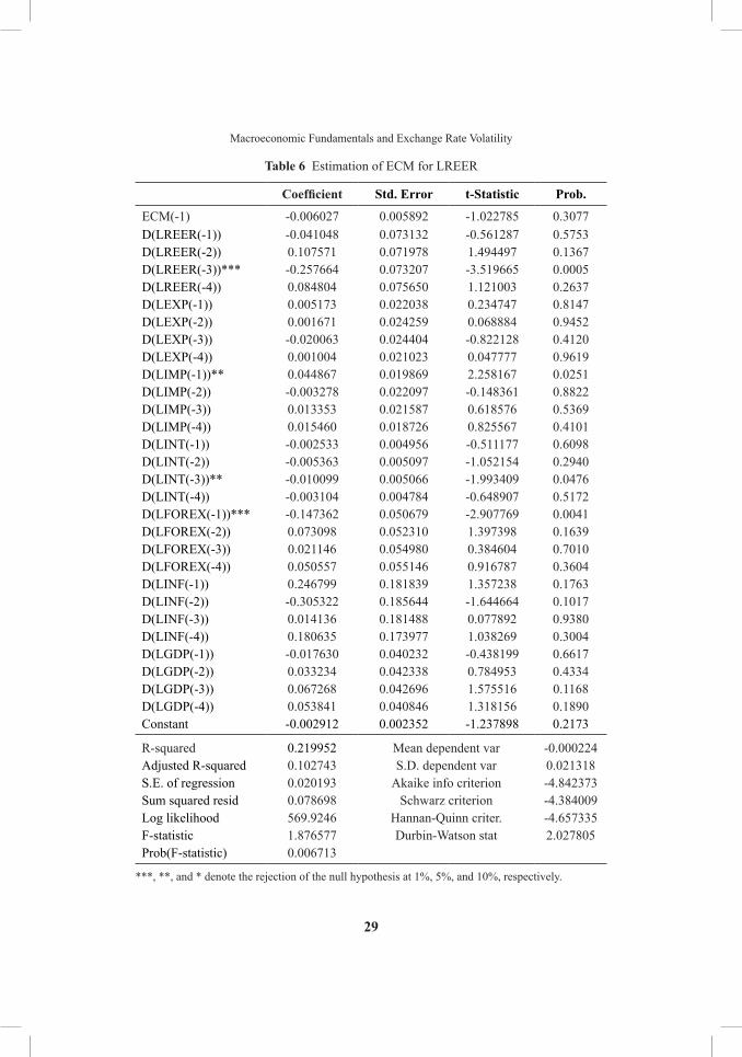
the result of the estimation of the error-correction model (ECM) for lrEEr is provided in table 6. It indicates that lrEEr has negative impact after a lag of 3 months and is highly significant at 1% level. This implies that the short-run real effective exchange rate is negatively influenced by its past values. Again, LIMP positively affects the variation of LREER at 5% level of significance after a lag of 1 month and LINT negatively influences the variation of the REER at 5% level of significance after a lag of 3 three months. LFOREX has negative impact on LREER at 1% level of significance after a lag of one month. Though volume of export (lEXp), domestic price level (lINF) and economic growth (lGdp) are the related macro variables with the LREER but any significant short-run impact of those variables on the lrEEr is not found in the present study.
29
Macroeconomic Fundamentals and Exchange Rate Volatility
Table 6 Estimation of ECM for lrEEr
Coefficient Std. Error t-Statistic prob.
ECM(-1) -0.006027 0.005892 -1.022785 0.3077d(lrEEr(-1)) -0.041048 0.073132 -0.561287 0.5753d(lrEEr(-2)) 0.107571 0.071978 1.494497 0.1367d(lrEEr(-3))*** -0.257664 0.073207 -3.519665 0.0005d(lrEEr(-4)) 0.084804 0.075650 1.121003 0.2637d(lEXp(-1)) 0.005173 0.022038 0.234747 0.8147d(lEXp(-2)) 0.001671 0.024259 0.068884 0.9452d(lEXp(-3)) -0.020063 0.024404 -0.822128 0.4120d(lEXp(-4)) 0.001004 0.021023 0.047777 0.9619d(lIMp(-1))** 0.044867 0.019869 2.258167 0.0251d(lIMp(-2)) -0.003278 0.022097 -0.148361 0.8822d(lIMp(-3)) 0.013353 0.021587 0.618576 0.5369d(lIMp(-4)) 0.015460 0.018726 0.825567 0.4101d(lINt(-1)) -0.002533 0.004956 -0.511177 0.6098d(lINt(-2)) -0.005363 0.005097 -1.052154 0.2940d(lINt(-3))** -0.010099 0.005066 -1.993409 0.0476d(lINt(-4)) -0.003104 0.004784 -0.648907 0.5172d(lFOrEX(-1))*** -0.147362 0.050679 -2.907769 0.0041d(lFOrEX(-2)) 0.073098 0.052310 1.397398 0.1639d(lFOrEX(-3)) 0.021146 0.054980 0.384604 0.7010d(lFOrEX(-4)) 0.050557 0.055146 0.916787 0.3604d(lINF(-1)) 0.246799 0.181839 1.357238 0.1763d(lINF(-2)) -0.305322 0.185644 -1.644664 0.1017d(lINF(-3)) 0.014136 0.181488 0.077892 0.9380d(lINF(-4)) 0.180635 0.173977 1.038269 0.3004d(lGdp(-1)) -0.017630 0.040232 -0.438199 0.6617d(lGdp(-2)) 0.033234 0.042338 0.784953 0.4334d(lGdp(-3)) 0.067268 0.042696 1.575516 0.1168d(lGdp(-4)) 0.053841 0.040846 1.318156 0.1890Constant -0.002912 0.002352 -1.237898 0.2173
r-squared 0.219952 Mean dependent var -0.000224Adjusted r-squared 0.102743 S.d. dependent var 0.021318S.E. of regression 0.020193 Akaike info criterion -4.842373Sum squared resid 0.078698 Schwarz criterion -4.384009log likelihood 569.9246 hannan-Quinn criter. -4.657335F-statistic 1.876577 durbin-watson stat 2.027805prob(F-statistic) 0.006713
***, **, and * denote the rejection of the null hypothesis at 1%, 5%, and 10%, respectively.
30
International Journal of Economics and Management
the readiness of misalignment of the rEEr from its long run equilibrium and its further adjustment towards the equilibrium can be judged with the help of the error-correction coefficient. The negative sign of the error correction coefficient indicates the correction of the disequilibrium situation. In the present study the estimated value of ECM (-1) carries the expected negative sign but it is not statistically significant. The Durbin-Watson statistic being 2 indicates that the residuals are uncorrelated with their lagged values i.e., there is no first-order serial correlation problem among the residuals.
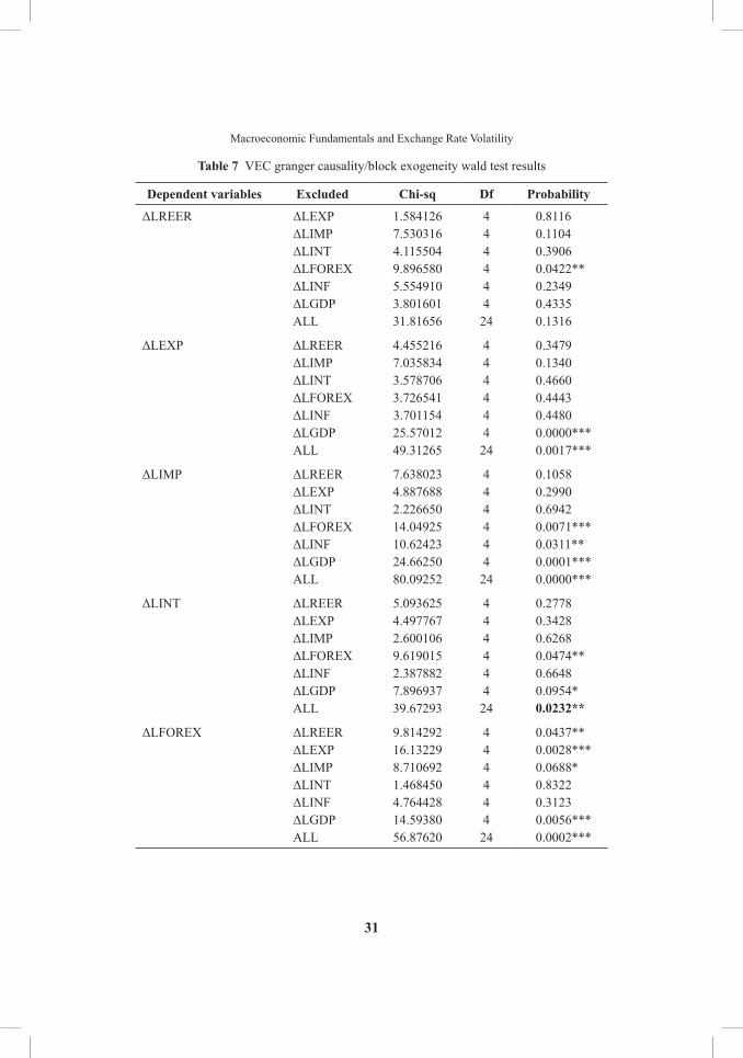
Now we have adopted the VEC Granger Causality/Block Exogeneity wald tests to examine the short-run causal relationship among the variables. table 7 indicates the results of causality test. the null hypothesis of block exogeneity is rejected for all equations in the model, except for ΔLREER. This indicates other than LREER each variable is jointly influenced by the other variables. We obtain five bi-directional causality as:
(i) ΔLREER ↔ ΔLFOREX
(ii) ΔLFOREX ↔ ΔLIMP
(iii) ΔLINF ↔ ΔLIMP
(iv) ΔLGDP ↔ ΔLIMP
(v) ΔLGDP ↔ ΔLINT
and six unidirectional causality as:
(i) ΔLGDP → ΔLEXP
(ii) ΔLFOREX → ΔLINT
(iii) ΔLEXP → ΔLFOREX
(iv) ΔLGDP → ΔLFOREX
(v) ΔLINT → ΔLINF
(vi) ΔLFOREX → ΔLINF
31
Macroeconomic Fundamentals and Exchange Rate Volatility
Table 7 VEC granger causality/block exogeneity wald test results
Dependent variables Excluded Chi-sq Df probability
ΔLREER ΔLEXP 1.584126 4 0.8116ΔLIMP 7.530316 4 0.1104ΔLINT 4.115504 4 0.3906ΔLFOREX 9.896580 4 0.0422**ΔLINF 5.554910 4 0.2349ΔLGDP 3.801601 4 0.4335All 31.81656 24 0.1316
ΔLEXP ΔLREER 4.455216 4 0.3479ΔLIMP 7.035834 4 0.1340ΔLINT 3.578706 4 0.4660ΔLFOREX 3.726541 4 0.4443ΔLINF 3.701154 4 0.4480ΔLGDP 25.57012 4 0.0000***All 49.31265 24 0.0017***
ΔLIMP ΔLREER 7.638023 4 0.1058ΔLEXP 4.887688 4 0.2990ΔLINT 2.226650 4 0.6942ΔLFOREX 14.04925 4 0.0071***ΔLINF 10.62423 4 0.0311**ΔLGDP 24.66250 4 0.0001***All 80.09252 24 0.0000***
ΔLINT ΔLREER 5.093625 4 0.2778ΔLEXP 4.497767 4 0.3428ΔLIMP 2.600106 4 0.6268ΔLFOREX 9.619015 4 0.0474**ΔLINF 2.387882 4 0.6648ΔLGDP 7.896937 4 0.0954*All 39.67293 24 0.0232**
ΔLFOREX ΔLREER 9.814292 4 0.0437**ΔLEXP 16.13229 4 0.0028***ΔLIMP 8.710692 4 0.0688*ΔLINT 1.468450 4 0.8322ΔLINF 4.764428 4 0.3123ΔLGDP 14.59380 4 0.0056***All 56.87620 24 0.0002***
32
International Journal of Economics and Management
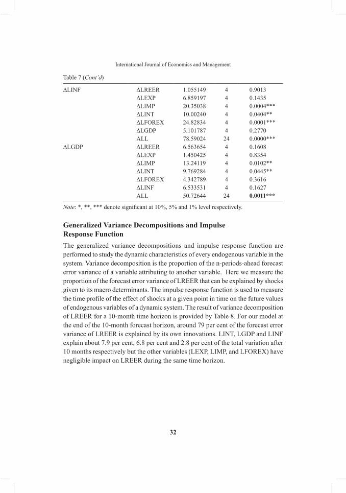
ΔLINF ΔLREER 1.055149 4 0.9013ΔLEXP 6.859197 4 0.1435ΔLIMP 20.35038 4 0.0004***ΔLINT 10.00240 4 0.0404**ΔLFOREX 24.82834 4 0.0001***ΔLGDP 5.101787 4 0.2770All 78.59024 24 0.0000***
ΔLGDP ΔLREER 6.563654 4 0.1608ΔLEXP 1.450425 4 0.8354ΔLIMP 13.24119 4 0.0102**ΔLINT 9.769284 4 0.0445**ΔLFOREX 4.342789 4 0.3616ΔLINF 6.533531 4 0.1627All 50.72644 24 0.0011***
Note: *, **, *** denote significant at 10%, 5% and 1% level respectively.
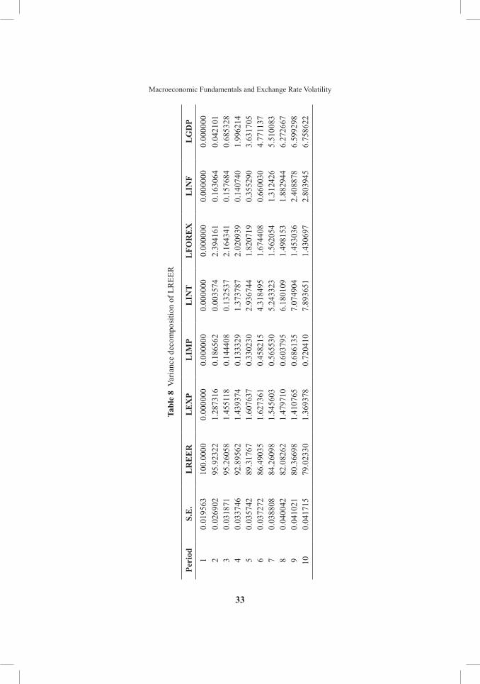
generalized Variance Decompositions and Impulse Response FunctionThe generalized variance decompositions and impulse response function are performed to study the dynamic characteristics of every endogenous variable in the system. Variance decomposition is the proportion of the n-periods-ahead forecast error variance of a variable attributing to another variable. here we measure the proportion of the forecast error variance of lrEEr that can be explained by shocks given to its macro determinants. the impulse response function is used to measure the time profile of the effect of shocks at a given point in time on the future values of endogenous variables of a dynamic system. the result of variance decomposition of LREER for a 10-month time horizon is provided by Table 8. For our model at the end of the 10-month forecast horizon, around 79 per cent of the forecast error variance of lrEEr is explained by its own innovations. lINt, lGdp and lINF explain about 7.9 per cent, 6.8 per cent and 2.8 per cent of the total variation after 10 months respectively but the other variables (lEXp, lIMp, and lFOrEX) have negligible impact on LREER during the same time horizon.
table 7 (Cont’d)
33
Macroeconomic Fundamentals and Exchange Rate Volatility
Tabl
e 8
Varia
nce
deco
mpo
sitio
n of
lr
EEr
peri
odS.
E.
lR
EE
Rl
Ex
pl
IMp
lIN
Tl
FOR
Ex
lIN
Fl
gD
p
10.
0195
6310
0.00
000.
0000
000.
0000
000.
0000
000.
0000
000.
0000
000.
0000
002
0.02
6902
95.9
2322
1.28
7316
0.18
6562
0.00
3574
2.39
4161
0.16
3064
0.04
2101
30.
0318
7195
.260
581.
4551
180.
1444
080.
1325
372.
1643
410.
1576
840.
6853
284
0.03
3746
92.8
9562
1.43
9374
0.13
3329
1.37
3787
2.02
0939
0.14
0740
1.99
6214
50.
0357
4289
.317
671.
6076
370.
3302
302.
9367
441.
8207
190.
3552
903.
6317
056
0.03
7272
86.4
9035
1.62
7361
0.45
8215
4.31
8495
1.67
4408
0.66
0030
4.77
1137
70.
0388
0884
.260
981.
5456
030.
5655
305.
2433
231.
5620
541.
3124
265.
5100
838
0.04
0042
82.0
8262
1.47
9710
0.60
3795
6.18
0109
1.49
8153
1.88
2944
6.27
2667
90.
0410
2180
.366
981.
4107
650.
6861
357.
0749
041.
4530
362.
4088
786.
5992
9810
0.04
1715
79.0
2330
1.36
9378
0.72
0410
7.89
3651
1.43
0697
2.80
3945
6.75
8622
34
International Journal of Economics and Management
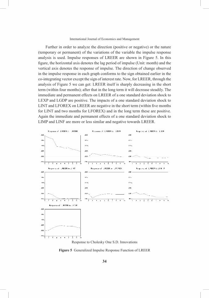
Further in order to analyze the direction (positive or negative) or the nature (temporary or permanent) of the variations of the variable the impulse response analysis is used. Impulse responses of lrEEr are shown in Figure 5. In this figure, the horizontal axis denotes the lag period of impulse (Unit: month) and the vertical axis denotes the response of impulse. the direction of change observed in the impulse response in each graph conforms to the sign obtained earlier in the co-integrating vector except the sign of interest rate. Now, for lrEEr, through the analysis of Figure 5 we can get: lrEEr itself is sharply decreasing in the short term (within four months); after that in the long term it will decrease steadily. the immediate and permanent effects on lrEEr of a one standard deviation shock to lEXp and lGdp are positive. the impacts of a one standard deviation shock to LINT and LFOREX on LREER are negative in the short term (within five months for lINt and two months for lFOrEX) and in the long term these are positive. Again the immediate and permanent effects of a one standard deviation shock to lIMp and lINF are more or less similar and negative towards lrEEr.
response to Cholesky One S.d. Innovations
Figure 5 Generalized Impulse Response Function of LREER
35
Macroeconomic Fundamentals and Exchange Rate Volatility
CONClUSIONthe study employs the Johansen co-integration and error correction model. Both the trace and maximum-eigenvalue co-integration tests suggest that there is positive long run relationship between India’s real effective exchange rate and its determinants. All the estimated coefficients carry the expected signs and are statistically significant. In addition each normalized co-integrating regression coefficient indicates long run elasticity of real effective exchange rate for respective parameter. In the long run real effective exchange rate responds strongly to all the variables except interest rate and foreign exchange reserve. In the short run, real effective exchange rate is determined by the specified lagged variables of its own, interest rate, level of foreign exchange reserves and import. Specifically, real effective exchange rate is negatively influenced by its own lags, interest rate and foreign exchange reserves, it is positively affected by import. VECM provides the error correction term which reflects the extent deviating from long-run equilibrium in the short-run. The error correction coefficient is -0.006027 and the direction is negative indicating when the short-run fluctuation of real effective exchange rate deviates from long-run equilibrium, the economic system will draw non-equilibrium state back to equilibrium state gradually at a very slow pace. to search for the nature of the short-run relationships among these variables, we have implemented the VEC Granger Causality/Block Exogeneity Wald Tests. Our results show five sets of strong evidences of the bi-directional and six sets of unidirectional causality. Generalized variance decompositions indicate that interest rate, economic growth and inflation have significant impact on real effective exchange rate. The direction of change observed in the impulse response in each graph conforms to the sign obtained earlier in the co-integrating vector except the sign of interest rate. Shocks to each of the determinants of real effective exchange rate have a long run impact on it.
So finally we can conclude that the overall macroeconomic developments and the pro-active role of the central bank such as timely changes in the monetary policy in several instances to maintain the exchange rate stability were effective to avoid wide fluctuation in the exchange rate even in the backdrop of East Asian currency crisis and most recently during the global financial crisis. There is surge of foreign capital inflow in India since the new economic reform but it has managed the exchange rate in such a way that real exchange rate has consistently fluctuated within a narrow band except very few cases. So it is rightly said that exchange rate management in India is more an art than science.
36
International Journal of Economics and Management
REFERENCESAsterious, d. and hall, S. (2007) Applied Econometrics: A Modern Approach. palgrave
Macmillan: london.Baccheta, p. and wincoop, E. Van. (2000) does Exchange rate Stability Increase trade and
welfare?, American Economic Review, 90(5), 1093-1109.Basurto, G. and Ghosh, A. (2000) the Interest rate-Exchange rate Nexus in the Asian Crisis
Countries”, working paper No. wp/00/19, International Monetary Fund.Calvo, G. and Mishkin, F. (2003) the Mirage of Exchange rate regimes for Emerging
Market Countries, Journal of Economic Perspectives, 17(4), 99-118.Chowdhury, r. (1993) does Exchange rate Volatility depress trade Flows? Evidence
from Error-Correction Models, The Review of Economics and Statistics, 75(4), 700-706.Crockett, A. and Goldstein, M. (1976) Inflation under Fixed and Flexible Exchange Rates,
IMF Staff papers, 23(1), 509-44.dell’ Ariccia, G. (1998) Exchange rate Fluctuations and trade Flows: Evidence from the
European union, IMF working paper, 98/107.Eichengreen, B. (2008) the real Exchange rate and Economic Growth, working paper
No.4, Commission on Growth and development, world Bank.Enders, w. ( 2004) Applied Econometric Time Series, 2nd Edition. John wiley & Sons:
New Jersey.Granger, C.w.J. and Newbold, p. (1974) Spurious regressions in Econometrics, Journal
of Econometrics, 2(1), 111-20.International Monetary Fund (2001) Annual report on Exchange rate Arrangements and
Exchange restrictions (washington).Johansen, S. (1988) Statistical Analysis of Cointegrating Vectors”, Journal of Economic
dynamics and Control, 12(2-3), 231–54.Johansen, S. and Juselius, K. (1990) Maximum likelihood Estimation and Inference on
Cointegration with Applications to the demand for Money, Oxford Bulletin of Economics and Statistics, 52(2), 169–210.
Johansen, S. (1991) Estimation and hypothesis testing of cointegration vectors in Gaussian vector autoregressive models, Econometrica, 59(6), 1551–80.
Johansen, S. and Juselius, K. (1992) testing Structural hypothesis in a Multivariate Cointegration Analysis of the ppp and uIp for uK, Journal of Econometrics, 53(1-3), 211–44.
Johansen, S. and Juselius, K. (1994) Identification of Long-run and Short-run Structure: An Application to the IS lM Model, Journal of Econometrics, 63(1), 7–36.
Johansen, S. (1995) likelihood-based Inference in Co-integrated Vector Autoregressive Models, Oxford: Oxford university press.
larrain, F. and Vergara, r. (1993) Investment and Macroeconomic Adjustment: the Case of East Asia. In : Serven l and Solimano A.,eds. Striving for Growth after Adjustment: the role of Capital Formation. washington, dC, world Bank, 229-74.
37
Macroeconomic Fundamentals and Exchange Rate Volatility
McKenzie, M. (1999) The Impact of Exchange Rate Volatility on International Trade Flows, Journal of Economic Surveys, 13(1), 71-106.
McKinnon, r. (1963) Optimum Currency Areas, American Economic Review, 53(4), 717-25.Neumeyer, p. and perri, F. (2005) Business Cycles in Emerging Economies:the role of Interest rates, Journal of Monetary Economics, 52(2), 345-80.reinhart, C. and reinhart, V. (2003) twin Fallacies about Exchange rate policy in Emerging
Markets, NBEr working paper Series, working paper, No. 9670, April 2003. rodrik, d. (2008) the real Exchange rate and Economic Growth, Brooking papers,
retrieved from www.brookings.edu/economics/bpea/bpea.aspx on on 11th May 2010.rostow, w. (1960) the Stages of Economic Growth: A Noncommunist Manifesto,
Cambridge: Cambridge university press.Schnable, G. (2007) Exchange rate Volatility and Growth in Small Open Economies at the
EMu periphery, working paper Series, No 773, European Central Bank.Solow, r. (1957) technical Change and the Aggregate production Function, Review of
Economics and Statistics, 39(3), 312-20.
38
International Journal of Economics and Management
App
EN
DIx
Tabl
e A.1
Sum
mar
y st
atis
tics,
tota
l sam
ple
Vari
able
No.
of
obse
rvat
ions
Mea
nM
edia
nM
axim
umM
inim
umSt
anda
rd
devi
atio
nSk
ewne
ssK
urto
sis
jarq
ue-
Ber
apr
obab
ility
lrEE
r22
84.
591
4.60
4.66
04.
470
0.04
1–0
.721
3.16
019
.999
0.00
0045
lEX
p22
810
.076
9.93
011
.860
8.56
00.
908
0.20
91.
880
13.5
810.
0011
24lI
Mp
228
10.3
4410
.095
12.3
08.
610
1.03
50.
214
1.83
814
.578
0.00
0683
lIN
t22
81.
893
1.90
3.55
0-0
.310
0.44
3–0
.205
6.97
815
2.07
30.
0000
00lF
Or
EX22
812
.629
12.6
5014
.290
10.3
901.
152
–0.1
071.
667
17.3
110.
0001
74lG
dp
228
5.22
25.
180
6.0
4.30
0.39
7–0
.075
2.35
34.
193
0.12
2895
lIN
F22
85.
134
5.12
05.
670
4.51
00.
293
–0.0
272.
146
6.95
50.
0308
91
39
Macroeconomic Fundamentals and Exchange Rate Volatility
Tabl
e A.2
lag
leng
th c
riter
ia re
sults
lag
log
ll
RFp
EA
ICSC
hQ
098
0.12
03N
A3.
68e-
13–8
.766
849
–8.6
5955
8–8
.723
532
126
11.7
9131
45.7
442.
36e-
19–2
3.02
515
–22.
1668
2*–2
2.67
861
227
06.2
4317
6.13
961.
57e-
19–2
3.43
462
–21.
8252
5–2
2.78
486*
327
55.4
7088
.696
751.
57e-
19–2
3.43
666
–21.
0762
5–2
2.48
368
428
08.1
3591
.571
201.
53e-
19*
–23.
4696
9*–2
0.35
823
–22.
2134
75
2855
.396
79.1
9468
*1.
57e-
19–2
3.45
402
–19.
5915
2–2
1.89
459
628
88.3
3153
.110
881.
84e-
19–2
3.30
929
–18.
6957
5–2
1.44
663
* in
dica
tes l
ag o
rder
sele
cted
by
the
crite
rion
LR: s
eque
ntia
l mod
ified
LR
test
stat
istic
(eac
h te
st a
t 5%
leve
l)Fp
E: F
inal
pre
dict
ion
erro
rA
IC: A
kaik
e in
form
atio
n cr
iterio
nSC
: Sch
war
z in
form
atio
n cr
iterio
nh
Q: h
anna
n-Q
uinn
info
rmat
ion
crite
rion