Macroeconomic Volatility and Stock Market Volatility,

World-Wide*

Francis X. DieboldUniversity of Pennsylvania

and NBER

Kamil Yilmaz†

Koc University

First draft: March 31, 2004This Revision/Print: August 6, 2008

Abstract: Notwithstanding its impressive contributions to empirical financial economics, thereremains a significant gap in the volatility literature, namely its relative neglect of the connectionbetween macroeconomic fundamentals and asset return volatility. We progress by analyzing abroad international cross section of stock markets covering approximately forty countries. Wefind a clear link between macroeconomic fundamentals and stock market volatilities, withvolatile fundamentals translating into volatile stock markets.

JEL classification: G1, E0

Key Words: Financial market, equity market, asset return, risk, variance, asset pricing

* We gratefully dedicate this paper to Rob Engle on the occasion of his 65th birthday. Theresearch was supported by the Guggenheim Foundation, the Humboldt Foundation, and theNational Science Foundation. For outstanding research assistance we thank Chiara Scotti andGeorg Strasser. For helpful comments we thank the Editor and Referee, as well as Joe Davis,Aureo DePaula, Jonathan Wright, and participants at the Penn Econometrics Lunch, theEconometric Society 2008 Winter Meetings in New Orleans, and the Engle FestschriftConference.

† Corresponding author:

Kamil YilmazDepartment of Economics Koc UniversityRumelifeneri Yolu, SariyerIstanbul 34450, TURKEYfax: +90 212 338 1653e-mail: kyilmaz@ku.edu.tr

1 The strongly positive volatility-volume correlation has received attention, as in Clark (1973),Tauchen (1983), and many others, but that begs the question of what drives volume, which again remainslargely unanswered.

2 By “fundamental volatility,” we mean the volatility of underlying real economic fundamentals. From the vantage point of a single equity, this would typically correspond to the volatility of real earningsor dividends. From the vantage point of the entire stock market, it would typically correspond to thevolatility of real GDP or consumption.

3 Another strand of macroeconomic literature, including for example Levine (1997), focuses on thelink between fundamental volatility and financial market development. Hence, although related, it toomisses the mark for our purposes.

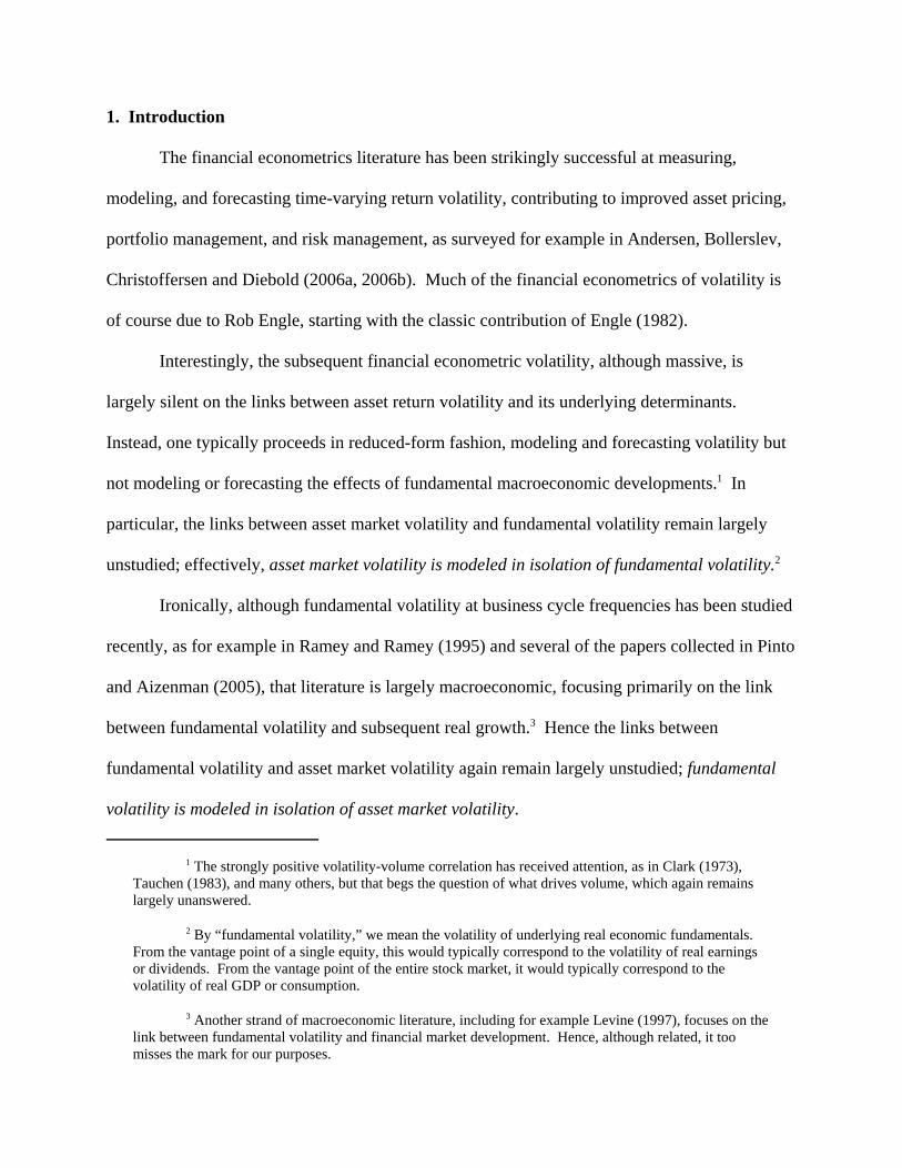
1. Introduction

The financial econometrics literature has been strikingly successful at measuring,

modeling, and forecasting time-varying return volatility, contributing to improved asset pricing,

portfolio management, and risk management, as surveyed for example in Andersen, Bollerslev,

Christoffersen and Diebold (2006a, 2006b). Much of the financial econometrics of volatility is

of course due to Rob Engle, starting with the classic contribution of Engle (1982).

Interestingly, the subsequent financial econometric volatility, although massive, is

largely silent on the links between asset return volatility and its underlying determinants.

Instead, one typically proceeds in reduced-form fashion, modeling and forecasting volatility but

not modeling or forecasting the effects of fundamental macroeconomic developments.1 In

particular, the links between asset market volatility and fundamental volatility remain largely

unstudied; effectively, asset market volatility is modeled in isolation of fundamental volatility.2

Ironically, although fundamental volatility at business cycle frequencies has been studied

recently, as for example in Ramey and Ramey (1995) and several of the papers collected in Pinto

and Aizenman (2005), that literature is largely macroeconomic, focusing primarily on the link

between fundamental volatility and subsequent real growth.3 Hence the links between

fundamental volatility and asset market volatility again remain largely unstudied; fundamental

volatility is modeled in isolation of asset market volatility.

4 Hansen and Jagannathan provide an inequality between the “Sharpe ratios” for the equity marketand the real fundamental and hence implicitly link equity volatility and fundamental volatility, other thingsequal.

-2-

Here we focus on stock market volatility. The general failure to link macroeconomic

fundamentals to asset return volatility certainly holds true for the case of stock returns. There

are few studies attempting to link underlying macroeconomic fundamentals to stock return

volatility, and the studies that do exist have been largely unsuccessful. For example, in a classic

and well-known contribution using monthly data from 1857 to 1987, Schwert (1989) attempts to

link stock market volatility to real and nominal macroeconomic volatility, economic activity,

financial leverage, and stock trading activity. He finds very little. Similarly and more recently,

using sophisticated regime-switching econometric methods for linking return volatility and

fundamental volatility, Calvet, Fisher and Thompson (2003) also find very little. The only

robust finding seems to be that the stage of the business cycle affects stock market volatility; in

particular, stock market volatility is higher in recessions, as found by Officer (1973) and echoed

in Schwert (1989) and Hamilton and Lin (1996), among others.

In this paper we provide an empirical investigation of the links between fundamental

volatility and stock market volatility. Our exploration is motivated by financial economic

theory, which suggests that the volatility of real activity should be related to stock market

volatility, as in Shiller (1981) and Hansen and Jagannathan (1991).4 In addition, and crucially,

our empirical approach exploits cross-sectional variation in fundamental and stock market

volatilities to uncover links that would likely be lost in a pure time series analysis.

Our paper is part of a nascent literature that explores the links between macroeconomic

fundamentals and stock market volatility. Engle and Rangel (2005) is a prominent example.

Engle and Rangel propose a spline-GARCH model to isolate low-frequency volatility, and they

5 Earlier drafts of our paper were completed contemporaneously with and independently of Engleand Rangel.

-3-

use the model to explore the links between macroeconomic fundamentals and low-frequency

volatility.5 Engle, Ghysels and Sohn (2006) is another interesting example, blending the spline-

GARCH approach with the mixed data sampling (MIDAS) approach of Ghysels, Santa-Clara,

and Valkanov (2005). The above-mentioned Engle et al. macro-volatility literature, however,

focuses primarily on dynamics, whereas in this paper we focus primarily on the cross section, as

we now describe.

2. Data

Our goal is to elucidate the relationship, if any, between real fundamental volatility and

real stock market volatility in a broad cross section of countries. To do so, we ask whether time-

averaged fundamental volatility appears linked to time-averaged stock market volatility. We

now describe our data construction methods in some detail; a more detailed description, along

with a complete catalog of the underlying data and sources, appears in the Appendix.

Fundamental and Stock Market Volatilities

First consider the measurement of fundamental volatility. We use data on real GDP and

real personal consumption expenditures (PCE) for many countries. The major source for both

variables is the World Development Indicators (WDI) of the World Bank.

We measure fundamental volatility in two ways. First, we calculate it as the standard

deviation of GDP (or consumption) growth, which is a measure of unconditional fundamental

volatility. Alternatively, following Schwert (1989), we use residuals from an AR(3) model fit to

GDP or consumption growth. This is a measure of conditional fundamental volatility, or put

6 The latter volatility measure is more relevant for our purposes, so we focus on it for theremainder of this paper. The empirical results are qualitatively unchanged, however, when we use theformer measure.

7 Again, however, we focus on the condition version for the remainder of this paper.

-4-

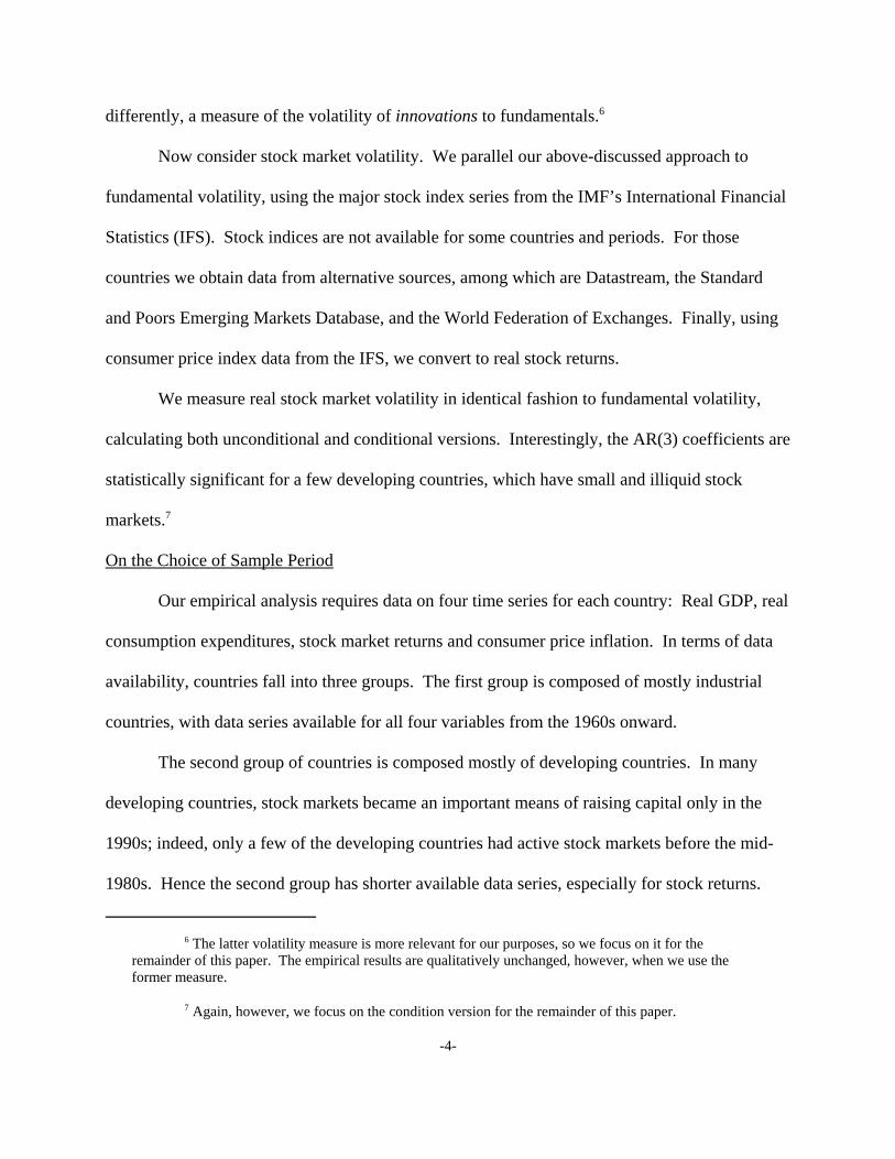
differently, a measure of the volatility of innovations to fundamentals.6

Now consider stock market volatility. We parallel our above-discussed approach to

fundamental volatility, using the major stock index series from the IMF’s International Financial

Statistics (IFS). Stock indices are not available for some countries and periods. For those

countries we obtain data from alternative sources, among which are Datastream, the Standard

and Poors Emerging Markets Database, and the World Federation of Exchanges. Finally, using

consumer price index data from the IFS, we convert to real stock returns.

We measure real stock market volatility in identical fashion to fundamental volatility,

calculating both unconditional and conditional versions. Interestingly, the AR(3) coefficients are

statistically significant for a few developing countries, which have small and illiquid stock

markets.7

On the Choice of Sample Period

Our empirical analysis requires data on four time series for each country: Real GDP, real

consumption expenditures, stock market returns and consumer price inflation. In terms of data

availability, countries fall into three groups. The first group is composed of mostly industrial

countries, with data series available for all four variables from the 1960s onward.

The second group of countries is composed mostly of developing countries. In many

developing countries, stock markets became an important means of raising capital only in the

1990s; indeed, only a few of the developing countries had active stock markets before the mid-

1980s. Hence the second group has shorter available data series, especially for stock returns.

8 On the “great moderation” in developed countries, see Kim and Nelson (1999), McConnell andPerez-Quiros (2000) and Stock and Watson (2002). Evidence for fundamental volatility moderation indeveloping countries also exists, although it is more mixed. For example, Montiel and Serven (2006) report

-5-

One could of course deal with the problems of the second group simply by discarding it,

relying only the cross section of industrialized countries. Doing so, however, would radically

reduce cross-sectional variation, producing potentially-severe reductions in statistical efficiency.

Hence we use all countries in the first and second groups, but we start our sample in 1983,

reducing the underlying interval used to calculate volatilities to 20 years.

The third group of countries is composed mostly of the transition economies and some

African and Asian developing countries, for which stock markets became operational only in the

1990s. As a result, we can include these countries only if we construct volatilities using roughly

a 10-year interval of underlying data. Switching from a 20-year to a 10-year interval, the

number of countries in the sample increases from around 40 to around 70 (which is good), but

using a 10-year interval produces much noisier volatility estimates (which is bad). We feel that,

on balance, the bad outweighs the good, so we exclude the third group of countries from our

basic analysis, which is based on underlying annual data. However, and as we will discuss, we

are able to base some of our analyses on underlying quarterly data, and in those cases we include

some of the third group of countries.

In closing this subsection, we note that, quite apart from the fact that data limitations

preclude use of pre-1980s data, use of such data would probably be undesirable even if it were

available. In particular, the growing literature on the “Great moderation” – decreased variation

of output around trend in industrialized countries, starting in the early 1980s – suggests the

appropriateness starting our sample in the early 1980s, so we take 1983-2002 as our benchmark

sample.8 Estimating fundamental volatility using both pre- and post-1983 data would mix

a decline in GDP growth volatility from roughly four percent in the 1970s and 1980s to roughly threepercent in the 1990s. On the other hand, Kose, Prasad, and Terrones (2006) find that developing countriesexperience increases in consumption volatility following financial liberalization, and many developingeconomies have indeed liberalized in recent years.

9 The approximate log-normality of volatility in the cross section parallels the approximateunconditional log-normality documented in the time series by Andersen, Bollerslev, Diebold and Ebens(2001).

10 We use the LOWESS locally-weighted regression procedure of Cleveland (1979).

-6-

observations from the high and low fundamental volatility eras, potentially producing distorted

inference.

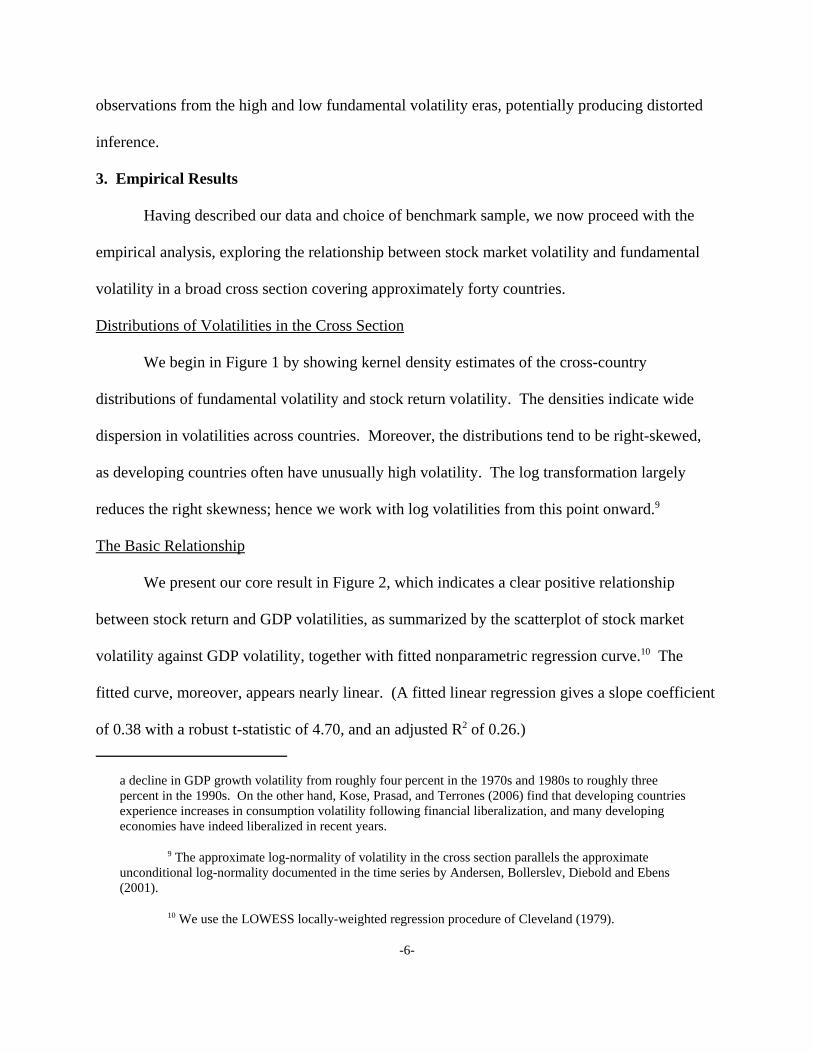
3. Empirical Results

Having described our data and choice of benchmark sample, we now proceed with the

empirical analysis, exploring the relationship between stock market volatility and fundamental

volatility in a broad cross section covering approximately forty countries.

Distributions of Volatilities in the Cross Section

We begin in Figure 1 by showing kernel density estimates of the cross-country

distributions of fundamental volatility and stock return volatility. The densities indicate wide

dispersion in volatilities across countries. Moreover, the distributions tend to be right-skewed,

as developing countries often have unusually high volatility. The log transformation largely

reduces the right skewness; hence we work with log volatilities from this point onward.9

The Basic Relationship

We present our core result in Figure 2, which indicates a clear positive relationship

between stock return and GDP volatilities, as summarized by the scatterplot of stock market

volatility against GDP volatility, together with fitted nonparametric regression curve.10 The

fitted curve, moreover, appears nearly linear. (A fitted linear regression gives a slope coefficient

of 0.38 with a robust t-statistic of 4.70, and an adjusted R2 of 0.26.)

-7-

When we swap consumption for GDP, the positive relationship remains, as shown in

Figure 3, although it appears less linear. In any event, the positive cross-sectional relationship

between stock market volatility and fundamental volatility contrasts with the Schwert’s (1989)

earlier-mentioned disappointing results for the U.S. time series.

Controlling for the Level of Initial GDP

Inspection of the country acronyms in Figures 2 and 3 reveals that both stock market and

fundamental volatilities are higher in developing (or newly industrializing) countries.

Conversely, industrial countries cluster toward low stock market and fundamental volatility.

This dependence of volatility on stage of development echoes the findings of Koren and

Tenreyro (2007) and has obvious implications for the interpretation of our results. In particular,

is it a development story, or is there more? That is, is the apparent positive dependence between

stock market volatility and fundamental volatility due to common positive dependence of

fundamental and stock market volatilities on a third variable, stage of development, or would the

relationship exist even after controlling for stage of development?

To explore this, we follow a two-step procedure. In the first step, we regress all variables

on initial GDP per capita, to remove stage-of-development effects (as proxied by initial GDP).

In the second step, we regress residual stock market volatility on residual fundamental volatility.

In Figures 4-6 we display the first-step regressions, which are of independent interest,

providing a precise quantitative summary of the dependence of all variables (stock market

volatility, GDP volatility and consumption volatility) on initial GDP per capita. The dependence

is clearly negative, particularly if we discount the distortions to the basic relationships caused by

India and Pakistan, which have very low initial GDP per capita, yet relatively low stock market,

and especially fundamental, volatility.

-8-

We display second-step results for the GDP fundamental in Figure 7. The fitted curve is

basically flat for low levels of GDP volatility, but it clearly becomes positive as GDP volatility

increases. A positive relationship also continues to obtain when we switch to the consumption

fundamental, as shown in Figure 8. Indeed the relationship between stock market volatility and

consumption volatility would be stronger after controlling for initial GDP if we were to drop a

single and obvious outlier (Philippines), which distorts the fitted curve at low levels of

fundamental volatility, as Figure 8 makes clear.

4. Variations and Extensions

Thus far we have studied stock market and fundamental volatility using underlying

annual data, 1983-2002. Here we extend our analysis in two directions. First, we incorporate

higher-frequency data when possible (quarterly for GDP and monthly, aggregated to quarterly,

for stock returns). Second, we use the higher frequency data in a panel-data framework to

analyze the direction of causality between stock market and fundamental volatility.

Cross-Sectional Analysis Based on Underlying Quarterly Data

As noted earlier, the quality of developing-country data starts to improve in the 1980s. In

addition, the quantity improves, with greater availability and reliability of quarterly GDP data.

We now use that quarterly data 1984:1 to 2003.3, constructing and examining volatilities over

four five-year spans: 1984.1-1988.4, 1989.1-1993.4, 1994.1-1998.4, and 1999.1-2003:3.

The number of countries increases considerably as we move through the four periods.

Hence let us begin with the fourth period, 1999.1-2003:3. We show in Figure 9 the fitted

regression of stock market volatility on GDP volatility. The relationship is still positive; indeed

it appears much stronger than the one discussed earlier, based on annual data 1983-2002 and

shown in Figure 2. Perhaps this is because the developing country GDP data have become less

11 Two outliers on the left (corresponding to Spain in the first two windows) distort the fitted curveand should be discounted.

12 There may of course also be bi-directional causality (feedback).

-9-

noisy in recent times.

Now let us consider the other periods. We obtained qualitatively identical results when

repeating the analysis of Figure 9 for each of the three earlier periods: Stock market volatility is

robustly and positively linked to fundamental volatility. To summarize those results compactly,

we show in Figure 10 the regression fitted to all the data, so that, for example, a country with

data available for all four periods has four data points in the figure. The positive relationship

between stock market and fundamental volatility is clear.11

Panel Analysis of Causal Direction

Thus far we have intentionally and exclusively emphasized the cross-sectional

relationship between stock market and fundamental volatility, and we found that the two are

positively related. However, economics suggests not only correlation between fundamentals and

stock prices, and hence from fundamental volatility to stock market volatility, but also (Granger)

causation.12

Hence in this sub-section we continue to exploit the rich dispersion in the cross section,

but we no longer average out the time dimension; instead, we incorporate it explicitly via a panel

analysis. Moreover, we focus on a particular panel analysis that highlights the value of

incorporating cross sectional information relative to a pure time series analysis. In particular, we

follow Schwert’s (1989) two-step approach to obtain estimates of time-varying quarterly stock

market and GDP volatilities, country-by-country, and then we test causal hypotheses in a panel

framework that facilitates pooling of the cross-country data.

-10-

Briefly, Schwert’s approach proceeds as follows. In the first step, we fit autoregressions

to stock market returns and GDP, and we take absolute values of the associated residuals, which

are effectively (crude) quarterly realized volatilities of stock market and fundamental

innovations, in the jargon of Andersen, Bollerslev, Diebold and Ebens (2001). In the second

stage, we transform away from realized volatilities and toward conditional volatilities by fitting

autoregressions to those realized volatilities, and keeping the fitted values. We repeat this for

each of the 46 countries.

We analyze the resulting 46 pairs of stock market and fundamental volatilities in two

ways. The first follows Schwert and exploits only time-series variation, estimating a separate

VAR model for each country and testing causality. The results, which are not reported here,

mirror Schwert’s, failing to identify causality in either direction in the vast majority of countries.

The second approach exploits cross-sectional variation along with time series variation.

We simply pool the data across countries, allowing for fixed effects. First we estimate a fixed-

effects model with GDP volatility depending on three lags of itself and three lags of stock

market volatility, which we use to test the hypothesis that stock market volatility does not

Granger cause GDP volatility. Next we estimate a fixed-effects model with stock market

volatility depending on three lags of itself and three lags of GDP volatility, which we use to test

the hypothesis that GDP volatility does not Granger cause Stock market volatility.

We report the results in Table 1, using quarterly real stock market volatility and real GDP

growth volatility for the panel of 46 countries, 1961.1 to 2003.3. We test non-causality from

fundamental volatility (FV) to return volatility (RV), and vice versa, and we present F-statistics

and corresponding p-values for both hypotheses. We do this for thirty sample windows, with the

ending date fixed at 2003.3 and the starting date varying from 1961.1, 1962.1, ..., 1990.1. There

13 Implied volatilities are generally not available.

-11-

is no evidence against the hypothesis that stock market volatility does not Granger cause GDP

volatility; that is, it appears that stock market volatility does not cause GDP volatility. In sharp

contrast, the hypothesis that GDP volatility does not Granger cause Stock market volatility is

overwhelmingly rejected: Evidently GDP volatility does cause stock market volatility.

The intriguing result of one-way causality from fundamental volatility stock return

volatility deserves additional study, as the forward-looking equity market might be expected to

predict macro fundamentals, rather than the other way around. Of course here we focus on

predicting fundamental and return volatilities, rather than fundamentals or returns themselves.

There are subtleties of volatility measurement as well. For example, we do not use implied stock

return volatilities, which might be expected to be more forward-looking.13

5. Concluding Remark

This paper is part of a broader movement focusing on the macro-finance interface. Much

recent work focuses on high-frequency data, and some of that work focuses on the high-

frequency relationships among returns, return volatilities and fundamentals (e.g., Andersen,

Bollerslev, Diebold and Vega, 2003, 2007). Here, in contrast, we focus on international cross

sections obtained by averaging over time. Hence this paper can be interpreted not only as

advocating more exploration of the fundamental volatility / return volatility interface, but also in

particular as a call for more exploration of volatility at medium (e.g., business cycle) frequencies.

In that regard it is to the stock market as, for example, Diebold, Rudebusch and Aruoba (2006) is

to the bond market and Evans and Lyons (2007) is to the foreign exchange market.

-12-

Appendix

Here we provide details of data sources, country coverage, sample ranges, and

transformations applied. We discuss underlying annual data first, followed by quarterly data.

Annual Data

We use four “raw” data series per country: Real GDP, real private consumption

expenditures (PCE), a broad stock market index, and the CPI. We use those series to compute

annual real stock returns, real GDP growth, real consumption growth, and corresponding

volatilities. The data set includes a total of 71 countries and spans a maximum of forty-two

years, 1960-2002. For many countries, however, consumption and especially stock market data

are available only for a shorter period, reducing the number of countries with data available.

We obtain annual stock market data from several sources, including International

Financial Statistics (IFS), the OECD, the International Finance Corporation (IFC) Emerging

Market Data Base (EMDB), Global Insight (accessed via WRDS), Global Financial Data,

Datastream, the World Federation of Exchanges, and various stock exchange web sites. Details

appear in Table A1, which lists the countries for which stock market index data are available at

least for the twenty-year period from 1983-2002. With stock prices in hand, we calculate

nominal returns as . We then calculate annual consumer price index (CPI)

inflation, , using the monthly IFS database 1960-2002, and finally we calculate real stock

returns as .

We obtain annual real GDP data from the World Bank World Development Indicators

database (WDI). For most countries, WDI covers the full 1960-2002 period. Exceptions are

Canada (data start in 1965), Germany (data start in 1971), Israel (data end in 2000), Saudi Arabia

(data end in 2001), and Turkey (data start in 1968). We obtain Taiwan real GDP from the

-13-

Taiwan National Statistics web site. We complete the real GDP growth rate series for Canada

(1961-65), Germany (1961-71), Israel (2001-2002) and Saudi Arabia (2002) using IFS data on

nominal growth and CPI inflation. We calculate real GDP growth rates as .

We obtain real personal consumption expenditures data using the household and personal

final consumption expenditure from the World Bank’s WDI database. We recover missing data

from the IFS and Global Insight (through WRDS); see Table A2 for details. We calculate real

consumption growth rates as .

Quarterly Data

The quarterly analysis reported in the text is based on 46 countries. Most, but not all, of

those countries are also included in the annual analysis.

For stock markets, we construct quarterly returns using the monthly data detailed in

Table A3, and we deflate to real terms using quarterly CPI data constructed using the same

underlying monthly CPI on which annual real stock market returns are based.

For real GDP in most countries, we use the IFS volume index. Exceptions are Brazil

(real GDP volume index, Brazilian Institute of Geography and Statistics website), Hong Kong

(GDP in constant prices, Census and Statistics Department website), Singapore (GDP in constant

prices, Ministry of Trade and Industry, Department of Statistics website), and Taiwan (GDP in

constant prices, Taiwan National Statistics website.

Table A4 summarizes the availability of the monthly stock index series and quarterly

GDP series for each country in our sample.

Table A1: Annual Stock Market Data

Country Period Covered Database / Source Acronyms

Argentina 1966 - 2002 1966 - 1989 Buenos Aires SE(1) General Index ARG1988 - 2002 Buenos Aires SE Merval Index

Australia 1961 - 2002 IFS (2) AUSAustria 1961 - 2002 1961 - 1998 IFS AUT

1999-2002 Vienna SE WBI indexBrazil 1980 - 2002 Bovespa SE BRACanada 1961 - 2002 IFS CANChile 1974 - 2002 IFS CHLColombia 1961 - 2002 IFS COLFinland 1961 - 2002 IFS FINFrance 1961 - 2002 IFS FRAGermany 1970 -2002 IFS GERGreece 1975 - 2002 Athens SE General Weighted Index GRCHong Kong, China 1965 - 2002 Hang Seng Index HKGIndia 1961 - 2002 IFS INDIndonesia 1977 - 2002 EMDB - JSE Composite (3) IDNIreland 1961 - 2002 IFS IRLIsrael 1961 - 2002 IFS ISRItaly 1961 - 2002 IFS ITAJamaica 1969 - 2002 IFS JAMJapan 1961 - 2002 IFS JPNJordan 1978 - 2002 Amman SE General Weighted Index JORKorea 1972 - 2002 IFS KORLuxembourg 1970 - 2002 1980 - 1998 IFS LUX

1999 - 2002 SE - LuxX General IndexMalaysia 1980 - 2002 KLSE Composite MYSMexico 1972 - 2002 Price & Quotations Index MEXMorocco 1980 - 2002 EMDB - Upline Securities MORNetherlands 1961 - 2002 IFS NLDNew Zealand 1961 - 2002 IFS NZLNorway 1961 - 2002 1961 - 2000 IFS NOR

2001 - 2002 OECD - CLI industrialsPakistan 1961 - 2002 1961 -1975 IFS PAK

1976 - 2002 EMDB- KSE 100Peru 1981 - 2002 Lima SE PERPhilippines 1961 - 2002 IFS PHLSingapore 1966 - 2002 1966 - 1979 Strait Times Old Index SGP

1980 - 2002 Strait Times New IndexSouth Africa 1961 - 2002 IFS SAFSpain 1961 - 2002 IFS SPASweden 1961 - 2002 IFS SWESwitzerland 1961 - 2002 OECD - UBS 100 index SWITaiwan 1967 - 2002 TSE Weighted Stock Index TAIThailand 1975 - 2002 SET Index THATrinidad and Tobago 1981 - 2002 EMDB - TTSE index TTBUnited Kingdom 1961 - 2002 1961 - 1998 IFS, industrial share index UK

1999 - 2002 OECD, industrial share indexUnites States 1961 - 2002 IFS USAVenezuela, Rep. Bol. 1961 - 2002 IFS VENZimbabwe 1975 - 2002 EMDB - ZSE Industrial ZBW

(1) SE denotes Stock Exchange.

(2) IFS denotes IMF’s International Financial Statistics. IFS does not provide the name of the stock market index.

(3) EMDB denotes Standard & Poors’ Emerging Market Data Base.

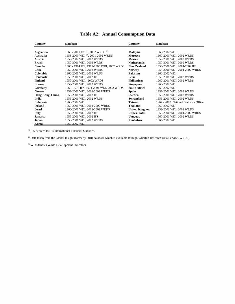
Table A2: Annual Consumption Data

Country Database Country Database

Argentina 1960 - 2001 IFS (1), 2002 WRDS (2) Malaysia 1960-2002 WDIAustralia 1958-2000 WDI (3), 2001-2002 WRDS Morocco 1960-2001 WDI, 2002 WRDSAustria 1959-2002 WDI, 2002 WRDS Mexico 1959-2001 WDI, 2002 WRDSBrazil 1959-2001 WDI, 2002 WRDS Netherlands 1959-2001 WDI, 2002 WRDSCanada 1960 - 1964 IFS; 1965-2000 WDI, 2002 WRDS New Zealand 1958-2000 WDI, 2001-2002 IFSChile 1960-2001 WDI, 2002 WRDS Norway 1958-2000 WDI, 2001-2002 WRDSColombia 1960-2001 WDI, 2002 WRDS Pakistan 1960-2002 WDIDenmark 1959-2001 WDI, 2002 IFS Peru 1959-2001 WDI, 2002 WRDSFinland 1959-2001 WDI, 2002 WRDS Philippines 1960-2001 WDI, 2002 WRDSFrance 1959-2001 WDI, 2002 WRDS Singapore 1960-2002 WDIGermany 1960 -1970 IFS, 1971-2001 WDI, 2002 WRDS South Africa 1960-2002 WDIGreece 1958-2000 WDI, 2001-2002 WRDS Spain 1959-2001 WDI, 2002 WRDSHong Kong, China 1959-2001 WDI, 2002 IFS Sweden 1959-2001 WDI, 2002 WRDSIndia 1959-2001 WDI, 2002 WRDS Switzerland 1959-2001 WDI, 2002 WRDSIndonesia 1960-2002 WDI Taiwan 1964 - 2002 National Statistics OfficeIreland 1960-2000 WDI, 2001-2002 WRDS Thailand 1960-2002 WDIIsrael 1960-2000 WDI, 2001-2002 WRDS United Kingdom 1959-2001 WDI, 2002 WRDSItaly 1959-2001 WDI, 2002 IFS Unites States 1958-2000 WDI, 2001-2002 WRDSJamaica 1959-2001 WDI, 2002 IFS Uruguay 1960-2001 WDI, 2002 WRDSJapan 1959-2001 WDI, 2002 WRDS Zimbabwe 1965-2002 WDIKorea 1960-2002 WDI

(1) IFS denotes IMF’s International Financial Statistics.

(2) Data taken from the Global Insight (formerly DRI) database which is available through Wharton Research Data Service (WRDS).

(3) WDI denotes World Development Indicators.

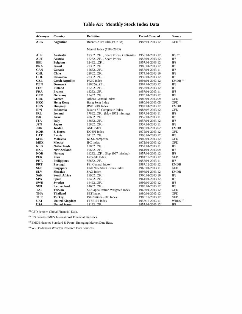
Table A3: Monthly Stock Index Data

Acronym Country Definition Period Covered Source

ARG Argentina Buenos Aires Old (1967-88)

Merval Index (1989-2003)

1983:01-2003:12 GFD (1)

AUS Australia 19362...ZF..., Share Prices: Ordinaries 1958:01-2003:12 IFS (2)

AUT Austria 12262...ZF..., Share Prices 1957:01-2003:12 IFSBEL Belgium 12462....ZF... 1957:01-2003:12 IFSBRA Brazil 22362...ZF... 1980:01-2003:12 IFSCAN Canada 15662...ZF... 1957:01-2003:11 IFSCHL Chile 22862...ZF... 1974:01-2003:10 IFSCOL Colombia 23362...ZF... 1959:01-2003:12 IFSCZE Czech Republic PX50 Index 1994:01-2003:12 EMDB (3)

DEN Denmark 12862A..ZF... 1967:01-2003:12 IFSFIN Finland 17262...ZF... 1957:01-2003:12 IFSFRA France 13262...ZF... 1957:01-2003:11 IFSGER Germany 13462...ZF... 1970:01-2003:12 IFSGRC Greece Athens General Index 1980:01-2003:09 GFDHKG Hong Kong Hang Seng Index 1980:01-2003:05 GFDHUN Hungary BSE BUX Index 1992:01-2003:12 EMDBIDN Indonesia Jakarta SE Composite Index 1983:03-2003:12 GFDIRL Ireland 17862...ZF... (May 1972 missing) 1957:01-2003:11 IFSISR Israel 43662...ZF... 1957:01-2003:11 IFSITA Italy 13662...ZF... 1957:01-2003:12 IFSJPN Japan 15862...ZF... 1957:01-2003:11 IFSJOR Jordan ASE Index 1986:01-2003:02 EMDBKOR S. Korea KOSPI Index 1975:01-2003:12 GFDLAT Latvia 94162...ZF... 1996:04-2003:12 IFSMYS Malaysia KLSE composite 1980:01-2003:12 GFDMEX Mexico IPC index 1972:01-2003:12 GFDNLD Netherlands 13862...ZF... 1957:01-2003:11 IFSNZL New Zealand 19662...ZF... 1961:01-2003:09 IFSNOR Norway 14262....ZF... (Sep 1997 missing) 1957:01-2003:12 IFSPER Peru Lima SE Index 1981:12-2003:12 GFDPHL Philippines 56662...ZF... 1957:01-2003:11 IFSPRT Portugal PSI General Index 1987:12-2003:12 EMDBSGP Singapore Old+New Strait Times Index 1966:01-2003:11 GFDSLV Slovakia SAX Index 1996:01-2003:12 EMDBSAF South Africa 19962...ZF... 1960:01-2003:10 IFSSPA Spain 18462...ZF... 1961:01-2003:12 IFSSWE Sweden 14462...ZF... 1996:06-2003:12 IFSSWI Switzerland 14662...ZF... 1989:01-2003:12 IFSTAI Taiwan SE Capitalization Weighted Index 1967:01-2003:12 GFDTHA Thailand SET Index 1980:01-2003:12 GFDTUR Turkey ISE National-100 Index 1986:12-2003:12 GFDUKI United Kingdom FTSE100 Index 1957:12-2003:11 WRDS (4)

USA United States 11162...ZF... 1957:01-2003:12 IFS

(1) GFD denotes Global Financial Data.(2) IFS denotes IMF’s International Financial Statistics. (3) EMDB denotes Standard & Poors’ Emerging Market Data Base. (4) WRDS denotes Wharton Research Data Services.

Table A4: Availability of Monthly Stock Returns and Quarterly GDP Series

Acronym Country 1984 I - 1988.IV 1989.I- 1993.IV 1994.I -1998.IV 1999.I - 2003.IV

Stock Index GDP Stock Index GDP Stock Index GDP Stock Index GDPARG Argentina T T T T T T T TAUS Australia T T T T T T TAUT Austria T T T T T T T TBEL Belgium T T T T T T T TBRA Brazil T T T T TCAN Canada T T T T T T T TCHL Chile T T T T T T T TCOL Colombia T T T T TCZE Czech Republic T T TDEN Denmark T T T T T T T TFIN Finland T T T T T T T TFRA France T T T T T T T TGER Germany T T T T T T T TGRC Greece T T T T THKG Hong Kong T T T T T THUN Hungary T T TIDN Indonesia T T T T TIRL Ireland T T T T TISR Israel T T T T T T T TITA Italy T T T T T T T TJPN Japan T T T T T T T TJOR Jordan T T T TKOR S. Korea T T T T T T T TLAT Latvia T TMYS Malaysia T T T T T T TMEX Mexico T T T T T T T TNLD Netherlands T T T T T T T TNZL New Zealand T T T T T T T TNOR Norway T T T T T T T TPER Peru T T T T T T T TPHL Philippines T T T T T T T TPRT Portugal T T T T T TSGP Singapore T T T T T T T TSLV Slovakia T TSAF South Africa T T T T T T T TSPA Spain T T T T T T T TSWE Sweden T TSWI Switzerland T T T T TTAI Taiwan T T T T T T T TTHA Thailand T T T TTUR Turkey T T T T T TUKI United Kingdom T T T T T T T TUSA United States T T T T T T T T

References

Andersen, T.G., Bollerslev, T., Christoffersen, P.F., and Diebold, F.X. (2006a), “Volatility and

Correlation Forecasting,” in G. Elliott, C.W.J. Granger, and A. Timmermann (eds.),

Handbook of Economic Forecasting. Amsterdam: North-Holland, 778-878.

Andersen, T.G., Bollerslev, T., Christoffersen, P.F. and Diebold, F.X. (2006b), “Practical

Volatility and Correlation Modeling for Financial Market Risk Management,” in M.

Carey and R. Stulz (eds.), Risks of Financial Institutions, University of Chicago

Press for NBER, 513-548.

Andersen, T., Bollerslev, T., Diebold, F.X. and Ebens, H. (2001), “The Distribution of Realized

Stock Return Volatility,” Journal of Financial Economics, 61, 43-76.

Andersen, T., Bollerslev, T., Diebold, F.X. and Vega, C. (2003), “Micro Effects of Macro

Announcements: Real-Time Price Discovery in Foreign Exchange,” American

Economic Review, 93, 38-62.

Andersen, T., Bollerslev, T., Diebold, F.X. and Vega, C. (2007), “Real-Time Price Discovery in

Stock, Bond and Foreign Exchange Markets,” Journal of International Economics,

73, 251-277.

Campbell, S.D and Diebold, F.X. (2008), “Stock Returns and Expected Business Conditions:

Half a Century of Direct Evidence,” Journal of Business and Economic Statistics, in

press.

Clark, P.K. (1973), “A Subordinated Stochastic Process Model with Finite Variance for

Speculative Prices,” Econometrica, 41, 135-155.

Cleveland, W.S. (1979), “Robust Locally Weighted Fitting and Smoothing Scatterplots,”

Journal of the American Statistical Association, 74, 829-836.

Diebold, F.X., Rudebusch, G.D. and Aruoba, B. (2006), “The Macroeconomy and the Yield

Curve: A Dynamic Latent Factor Approach,” Journal of Econometrics, 131,

309-338.

Engle, R.F. (1982), “Autoregressive Conditional Heteroscedasticity with Estimates of the

Variance of United Kingdom Inflation,” Econometrica, 50, 987-1007.

Engle, R.F., Ghysels, E. and Sohn, B. (2006), “On the Economic Sources of Stock Market

Volatility,” Manuscript, New York University.

Engle, R.F. and Rangel, J.G. (2008), “The Spline Garch Model for Unconditional Volatility and

Its Global Macroeconomic Causes,” Review of Financial Studies, in press.

Evans, M.D.D. and Lyons, R.K. (2007), “Exchange Rate Fundamentals and Order Flow,”

Manuscript, Georgetown University and University of California, Berkeley.

Ghysels, E., Santa-Clara, P. and R. Valkanov (2006), “Predicting Volatility: How to Get the

Most Out of Returns Data Sampled at Different Frequencies,” Journal of

Econometrics, 131, 59-95.

Hamilton, J.D. and Lin, G. (1996), “Stock Market Volatility and the Business Cycle,” Journal of

Applied Econometrics, 11, 573-593.

Hansen, L.P and Jagannathan, R. (1991), “Implications of Security Market Data for Models of

Dynamic Economies,” Journal of Political Economy, 99, 225-262.

Kim C.J. and Nelson, C.R. (1999), “Has the US Economy Become More Stable? A Bayesian

Approach Based on a Markov-Switching Model of the Business Cycle,” Review of

Economics and Statistics, 81, 608-616.

Koren , M. and Tenreyro, S. (2007), “Volatility and Development,” Quarterly Journal of

Economics, 122, 243-287.

Kose, M.A., Prasad, E.S. and Terrones, M.E. (2006), “How Do Trade and Financial Integration

Affect the Relationship Between Growth and Volatility?,” Journal of International

Economics, 69, 176-202.

Levine, R. (1997), “Financial Development and Economic Growth: Views and Agenda,”

Journal of Economic Literature, 35, 688-726.

McConnell, M.M. and Perez-Quiros, G. (2000), “Output Fluctuations in the United States:

What Has Changed Since the Early 1980s?,” American Economic Review, 90, 1464-

1476.

Montiel, P. and Serven, L. (2006), “Macroeconomic Stablity in Developing Countries: How

Much is Enough?,” The World Bank Research Observer, 21, fall, 151-178.

Pinto, B. and Aizenman, J. (eds.) (2005), Managing Economic Volatility and Crises: A

Practitioner's Guide. Cambridge: Cambridge University Press.

Ramey, G. and Ramey, V.A. (1995), “Cross-country Evidence on the Link Between Volatility

and Growth,” American Economic Review, 85, 1138–1151.

Schwert, G.W. (1989), “Why Does Stock Market Volatility Change Over Time?,” Journal of

Finance, 44, 1115-1153.

Shiller, R.J. (1981), “Do Stock Prices Move Too Much to be Justified by Subsequent Changes in

Dividends?,” American Economic Review, 71, 421–436.

Stock, J.H. and Watson, M.W. (2002), “Has the Business Cycle Changed and Why?,” in M.

Gertler and K. Rogoff (eds.), NBER Macroeconomics Annual 2002. Cambridge,

Mass.: MIT Press.

Tauchen, G. (1983), “The Price Variability-Volume Relationship on Speculative Markets,”

Econometrica, 51, 485-506.

Figure 1. Kernel Density Estimates, Volatilities and Fundamentals, 1983-2002 Real Stock Return Volatility Log Real Stock Return Volatility

Real GDP Growth Volatility Log Real GDP Growth Volatility

Real PCE Growth Volatility Log Real PCE Growth Volatility

0

.01

.02

.03

.04

Den

sity

10 20 30 40 50sdreret20xx

Log Real PCE Growth Volatility

0

.2

.4

.6

.8

1

Den

sity

2 2.5 3 3.5 4lsdreret20xx

Log Real PCE Growth Volatility

0

.2

.4

.6

.8

Den

sity

0 .5 1 1.5 2lsdingdpgr20xx

Log Real PCE Growth Volatility

0

.1

.2

.3

Den

sity

0 2 4 6 8sdingdpgr20xx

Log Real PCE Growth Volatility

0

.05

.1

.15

.2

.25

Den

sity

0 2 4 6 8 10sdinpcegr20xx

Log Real PCE Growth Volatility

0

.2

.4

.6

Den

sity

-1 0 1 2 3lsdinpcegr20xx

Log Real PCE Growth Volatility

Figure 2. Real Stock Return Volatility and Real GDP Growth Volatility, 1983-2002

NLD

ITA

SWI

UK

SPA

FRAGER

AUT

NOR

USA

JPN

PAK

AUS

SWE

GRC

CAN

NZL

IND

COL

FIN

ISR

SAF

TAI

IRL

JAMLUX

BRAPHL

CHL

TTB

MEX

KOR

HKGSGP

THA

MOR

MYS

IDN

JOR

VEN

ZBW PERARG

2

2.5

3

3.5

4

Log

Rea

l Sto

ck R

etur

n V

olat

ility

0 .5 1 1.5 2Log Real GDP Growth Volatilityxx

Locally-weighted least squares estimates

Figure 3. Real Stock Return Volatility and Real PCE Growth Volatility, 1983-2002

SWI

FRAJPN

USA

NLD

CAN

GER

AUT

AUS

UK

PHL

SPA

SWEITA

NOR

GRC

IND

IRL

NZL

FIN

SAF

TAI

COL SGP

PAK

BRA

ISRHKG

MEX

THA

KOR

CHL

MOR

MYS

PERIDNARG

JAM

ZBW

2

2.5

3

3.5

4

Log

Rea

l Sto

ck R

etur

n V

olat

ility

0 .5 1 1.5 2Log Real PCE Growth Volatilityxx

Locally-weighted least squares estimates

Figure 4. Real Stock Return Volatility and Initial Real GDP Per Capita, 1983-2002

IND

PAK

IDNZBW

MOR

THA

PHL

COL

JOR

JAM

CHL

MYS

PERTAI

MEX

VEN

BRA

KOR

SAF

TTB

ARG GRC

SPA

IRL

SGPISRHKG

UK

NZL

ITA

AUS

CAN

NLD

USA

FIN

FRA

AUTSWE

GERNOR

LUX

JPN

SWI

2

2.5

3

3.5

4

Log

Rea

l Sto

ck R

etur

n V

olat

ility

6 8 10 12Log Real GDP per capita in 1983xx

Locally-weighted least squares estimates

Figure 5. Real GDP Growth Volatility and Initial GDP Per Capita, 1983-2002

IND

PAK

IDN

ZBW

MORTHA

PHL

COL

JOR

JAMCHL

MYS

PER

TAI

MEX

VEN

BRA

KOR

SAF

URY

TTB

ARG

GRC

SPA

IRL

SGP

ISR

HKG

UK

NZL

ITA

AUS

CAN

NLD

USA

FIN

FRAAUT

SWE

GERNOR

LUX

DENJPN

SWI

0

.5

1

1.5

2

Log

Rea

l GD

P G

row

th V

olat

ility

6 8 10 12Log Real GDP per capita in 1983xx

Locally-weighted least squares estimates

Figure 6. Real PCE Growth Volatility and Initial GDP Per Capita, 1983-2002

IND

PAK

IDN

ZBW

MOR

THA

PHL

COL

JAM

CHLMYSPER

TAI

MEX

BRA

KOR

SAF

URYARG

GRCSPA

IRL

SGPISRHKG

UK

NZL

ITA

AUSCAN

NLDUSA

FIN

FRA

AUT

SWE

GER

NORDEN

JPN SWI

0

.5

1

1.5

2

Log

Rea

l PC

E G

row

th V

olat

ility

6 8 10 12Log Real GDP per capita in 1983xx

Locally-weighted least squares estimates

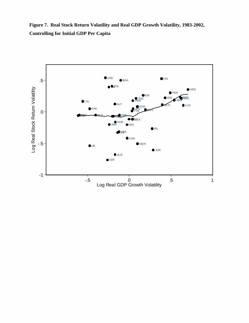
Figure 7. Real Stock Return Volatility and Real GDP Growth Volatility, 1983-2002,

Controlling for Initial GDP Per Capita

COLSPA

ITA

UK

PAK

NLD

GRC

SAF

TAI

JAM

PHL

FRAGER

AUT

AUS

NOR

CHLUSA

SWI

BRA

IND

CAN

NZL

TTB

MEX

SWE

JPN

THA

KOR

MOR

ISR

MYS

IRL

JOR

FIN

VEN

IDN

PER

ZBWSGPHKG

LUX

ARG

-1

-.5

0

.5

Log

Rea

l Sto

ck R

etur

n V

olat

ility

-.5 0 .5 1Log Real GDP Growth Volatilityxx

Locally-weighted least squares estimates

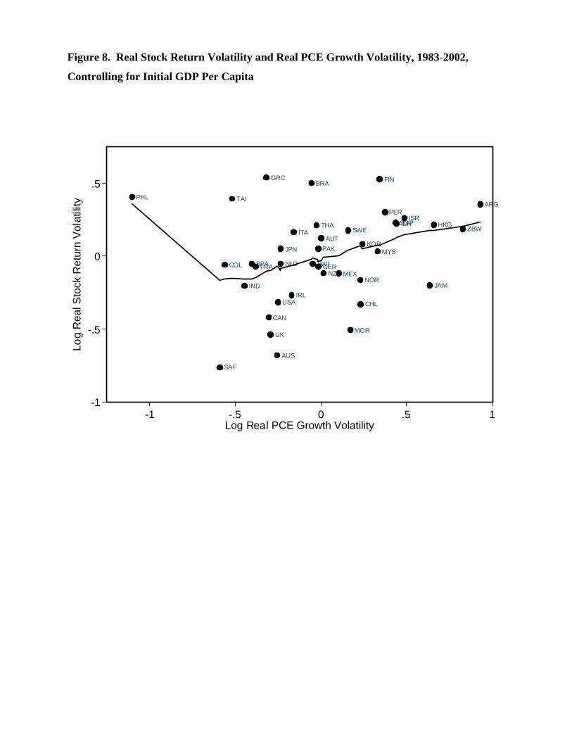
Figure 8. Real Stock Return Volatility and Real PCE Growth Volatility, 1983-2002,

Controlling for Initial GDP Per Capita

PHL

SAF

COL

TAI

IND

SPAFRA

GRC

CAN

UK

AUS

USA

JPN

NLD

IRL

ITA

BRA

SWI

THA

PAK

GER

AUT

NZL MEX

SWE

MOR

NOR

CHL

KORMYS

FIN

PERSGPIDN

ISR

JAM

HKG ZBW

ARG

-1

-.5

0

.5

Log

Rea

l Sto

ck R

etur

n V

olat

ility

-1 -.5 0 .5 1Log Real PCE Growth Volatilityxx

Locally-weighted least squares estimates

Figure 9. Real Stock Return Volatility and Real GDP Growth Volatility, 1999.I-2003.III

UKISAF

NLD

SWI

HUN

CAN

GER

USA

CZE

AUS

ITA

DENCOL

NZL

MEX

FIN

SLV

AUT

JPN

SPA

PHL

CHL

SWEFRA

PRT

IDN

BEL

THA

NOR

MYS

LAT

TAI

HKG

SGP

IRL

KOR

ISR

PER

TUR

ARG

1.5

2

2.5

3

3.5

Log

Rea

l Sto

ck R

etur

n V

olat

ility

-1 0 1 2Log Real GDP Growth Volatilityxx

Locally-weighted least squares estimates

Figure 10. Real Stock Return Volatility and Real GDP Growth Volatility, 1984:I-2003.III

1.5

22.

53

3.5

Log

Rea

l Sto

ck R

etur

n V

olat

ility

-1 0 1 2Log Real GDP Growth Volatilityxx

Lowess smoother

Table 1. Granger Causality Analysis of Stock Market Volatility and Fundamental Volatility

BeginningYear RV not Y FV FV not Y RV

F-stat. p-value F-stat. p-value1961 1.16 0.3264 4.14 0.00241962 1.18 0.3174 4.09 0.00261963 1.11 0.3498 4.21 0.00211964 1.14 0.3356 4.39 0.00151965 1.07 0.3696 4.33 0.00171966 1.06 0.3746 4.33 0.00171967 1.01 0.4007 4.48 0.00131968 1.00 0.4061 4.44 0.00141969 0.98 0.4171 4.38 0.00161970 0.96 0.4282 4.14 0.00241971 0.89 0.4689 3.86 0.00391972 0.78 0.5380 4.16 0.00231973 0.62 0.6482 4.06 0.00271974 0.84 0.4996 4.40 0.00151975 0.83 0.5059 3.90 0.00361976 0.83 0.5059 3.89 0.00371977 0.95 0.4339 3.93 0.00351978 0.88 0.4750 4.11 0.00251979 0.73 0.5714 4.02 0.00301980 0.74 0.5646 4.52 0.00121981 0.49 0.7431 4.67 0.00091982 0.47 0.7578 4.77 0.00081983 0.59 0.6699 5.15 0.00041984 0.71 0.5850 5.39 0.00031985 0.83 0.5059 5.58 0.00021986 1.07 0.3697 5.59 0.00021987 1.29 0.2716 5.76 0.00011988 1.29 0.2716 4.84 0.00071989 1.21 0.3044 3.86 0.00391990 1.23 0.2959 3.42 0.0085

Notes to Figures and Tables

Figure 1. We plot kernel density estimates of real stock return volatility (using data for 43

countries), real GDP growth volatility (45 countries), and real consumption growth volatility (41

countries), in both levels and logs. All volatilities are standard deviations of residuals from

AR(3) models fitted to annual data, 1983-2002. For comparison we also include plots of best-

fitting normal densities (dashed).

Figure 2. We show a scatterplot of real stock return volatility against real GDP growth

volatility, with a nonparametric regression fit superimposed, for 43 countries. All volatilities are

log standard deviations of residuals from AR(3) models fitted to annual data, 1983-2002.

Figure 3. We show a scatterplot of real stock return volatility against real consumption growth

volatility, with a nonparametric regression fit superimposed, for 39 countries. All volatilities are

log standard deviations of residuals from AR(3) models fitted to annual data, 1983-2002.

Figure 4. We show a scatterplot of real stock return volatility against initial (1983) real GDP

per capita, with a nonparametric regression fit superimposed, for 43 countries. All volatilities

are log standard deviations of residuals from AR(3) models fitted to annual data, 1983-2002.

Figure 5. We show a scatterplot of real GDP growth volatility against initial (1983) real GDP

per capita, with a nonparametric regression fit superimposed, for 45 countries. All volatilities

are log standard deviations of residuals from AR(3) models fitted to annual data, 1983-2002.

The number of countries is two more than in Figure 2 because we include Uruguay and Denmark

here, whereas we had to exclude them from Figure 2 due to missing stock return data.

Figure 6. We show a scatterplot of real consumption growth volatility against initial (1983) real

GDP per capita, with a nonparametric regression fit superimposed, for 41 countries. All

volatilities are log standard deviations of residuals from AR(3) models fitted to annual data,

1983-2002. The number of countries is two more than in Figure 3 because we include Uruguay

and Denmark here, whereas we had to exclude them from Figure 3 due to missing stock return

data.

Figure 7. We show a scatterplot of real stock return volatility against real GDP growth volatility

with a nonparametric regression fit superimposed, for 43 countries, controlling for the effects of

initial GDP per capita via separate first-stage nonparametric regressions of each variable on 1983

GDP per capita. All volatilities are log standard deviations of residuals from AR(3) models

fitted to annual data, 1983-2002.

Figure 8. We show a scatterplot of real stock return volatility against real consumption growth

volatility with a nonparametric regression fit superimposed, for 39 countries, controlling for the

effects of initial GDP per capita via separate first-stage nonparametric regressions of each

variable on 1983 GDP per capita. All volatilities are log standard deviations of residuals from

AR(3) models fitted to annual data, 1983-2002.

Figure 9. We show a scatterplot of real stock return volatility against real GDP growth

volatility, with a nonparametric regression fit superimposed, for 40 countries. All volatilities are

log standard deviations of residuals from AR(4) models fitted to quarterly data, 1999.1-2003.3.

Figure 10. We show a scatterplot of real stock return volatility against real GDP growth

volatility, with a nonparametric regression fit superimposed, for 43 countries. All volatilities are

log standard deviations of residuals from AR(4) models fitted to quarterly data over four

consecutive five-year windows (1984.1-1988.4, 1989.1-1993.4,1994.1-1998.4,1999.1-2003.3).

Table 1. We assess the direction of causal linkages between quarterly real stock market

volatility and real GDP growth volatility for the panel of 46 countries, 1961.1 to 2003.3. We test

non-causality from fundamental volatility (FV) to return volatility (RV), and vice versa, and we

present F-statistics and corresponding p-values for both hypotheses. We do this for thirty sample

windows, with the ending date fixed at 2003.3 and the starting date varying from 1961.1, 1962.1,

..., 1990.1.