Embed Size (px)
DESCRIPTION
Citation preview

NRG WORKING PAPER SERIES
STOCK MARKET VOLATILITY AND MACROECONOMICUNCERTAINTY
EVIDENCE FROM SURVEY DATA
Ivo J.M. Arnold, Evert B. VrugtMarch 2006 no. 06-08Nyenrode Research Group

NRG WORKING PAPER SERIES
Stock Market Volatility and Macroeconomic Uncertainty
Evidence from Survey Data
Ivo J.M. Arnold Evert B. Vrugt
March 2006
NRG Working Paper no. 06-08
NRG
The Nyenrode Research Group (NRG) is a research institute consisting of researchers from Nyenrode Business Universiteit and Hogeschool
INHOLLAND, within the domain of Management and Business Administration.
Straatweg 25, 3621 BG Breukelen P.O. Box 130, 3620 AC Breukelen The Netherlands Tel: +31 (0) 346 - 291 696 Fax: +31 (0) 346 - 291 250 E-mail: [email protected] NRG working papers can be downloaded at http://www.nyenrode.nl/research/publications

Abstract This paper provides empirical evidence on the link between stock market volatility and macroeconomic uncertainty. We show that US stock market volatility is significantly related to the dispersion in economic forecasts from SPF survey participants over the period from 1969 to 1996. This link is much stronger than that between stock market volatility and the more traditional time-series measures of macroeconomic volatility, but disappears after 1996. Keywords Stock market volatility, macro-economic factors, survey data JEL codes E44, G12 Address for correspondence Ivo J.M. Arnold (corresponding author) Universiteit Nyenrode, Straatweg 25, 3621 BG, The Netherlands E-mail: [email protected] Evert B. Vrugt ABP Investments, Amsterdam, The Netherlands E-mail: [email protected] The views expressed in this paper do not necessarily reflect the views of ABP Investments.
2

1. Introduction
The link between the macroeconomy and the stock market has intuitive appeal, as
macroeconomic variables affect both expected cash flows accruing to stockholders and
discount rates. A common theoretical framework connecting stock prices to fundamentals is
the dividend discount model. According to this model, new macroeconomic information will
affect stock prices if it impacts on either expectations about future dividends, discount rates,
or both.
Empirically, the evidence linking macroeconomic factors to the stock market is mixed at
best. Chen, Roll, and Ross (1986) were one of the first to explore the link between
macroeconomic variables and stock prices. Using a multifactor model, they found evidence
that macroeconomic factors are priced. Pearce and Roley (1985), Hardouvelis (1987) and
Cutler, Potterba and Summers (1989) also conclude that stock prices respond to
macroeconomic news. Subsequent studies have produced more mixed results. While some
studies confirmed Chen, Roll and Ross’s (1986) findings (see e.g McElroy and Burmeister,
1988, Hamao, 1988), others have been less successful (see e.g Poon and Taylor, 1991,
Shanken, 1992).
Moving from first to second moments, Veronesi (1999) presents a theoretical model that
formalizes the link between economic uncertainty and stock market volatility. He shows that
investors are more sensitive to news during periods of high uncertainty, which in turn
increases asset price volatility. Yet establishing the empirical link between the second
moments of stock returns and macroeconomic variables has proven to be even more
challenging than that between their first moments. Based on US data, Schwert (1989)
concludes that there is a volatility puzzle (p. 1146):
“The puzzle highlighted by the results in this paper is that stock volatility is not more closely related to other
measures of economic volatility.”

In examining which factors drive systematic stock return covariation, Chan, Karceski and
Lakonishok (1998) even conclude (p. 182):
“... the macroeconomic factors do a poor job in explaining return covariation. In terms of understanding the
return covariation across stocks, widely used factors such as industrial production growth and unanticipated
inflation do not seem to be more useful than a randomly generated series of numbers.”
There are a few exceptions to this negative finding, mainly for countries or periods where
macroeconomic volatility has been higher than in the US. For Europe, Errunza and Hogan
(1998) find a significant influence of monetary and real macroeconomic volatility on stock
market volatility for the seven largest European countries. Bittlingmayer (1998) finds
significant effects of economic and political uncertainty on German stock market volatility
for the period 1880–1940, yet this period includes rather dramatic economic and politicial
circumstances and may thus not be representative for more stable times.
Given the poor results in explaining stock market volatility, at least for the US, a more recent
branch of the literature focuses on identifying the effect of macroeconomic announcements
on asset volatility using high frequency data, see e.g. Jones, Lamont and Lumsdaine (1998)
for fixed income, Andersen et al. (2003) for foreign exchange and Flannery and
Protopapadakis (2002) for equities. Using dummies to account for days with macroeconomic
announcements, this approach is more successful in linking macroeconomic news to asset
volatility. It has been difficult, however, to establish this link beyond the daily-frequency
domain.
Starting with Schwert (1989), the most common way to extract macroeconomic volatility is
by means of a time-series model. The absolute residuals from autoregressive models fitted
on stock returns and macroeconomic growth rates are typically used as volatility estimates.
But there are some limitations to this approach, see also Giordani and Söderlind (2003).
First, a major concern is that time-series models are backward looking, whereas most
applications are about ex-ante uncertainty. Second, time-series measures present problems
when time-series are subject to structural breaks. Third, there is no universal time-series
model to extract expectations. Different models will thus yield different uncertainty
4
estimates leading to different empirical outcomes. The fourth and, we believe, most
important limitation is that time-series volatility captures the volatility in just one single ex-
post realization of macroeconomic developments out of many possible ex-ante scenarios.
One realized path of macroeconomic growth rates may appear smooth ex-post,
notwithstanding significant ex-ante uncertainty as to which path would occur. The time-
series dimension of the data will not capture this notion of uncertainty adequately. In this
context, Robert Merton has interpreted the Great Depression as an example of the “Peso
problem” (see Schwert (1989). At that time, there was significant uncertainty whether the
economic system as a whole would survive, which is not apparent by looking at the ex-post
data. A similar reasoning has been applied by Kleidon (1986) on the excess volatility puzzle,
where actual stock prices appear to be much too volatile compared to the smooth patterns in
ex-post dividends which we observe.
In this paper, we provide new empirical evidence on the link between stock market volatility
and macroeconomic uncertainty. We show that stock market volatility is significantly related
to the dispersion in economic forecasts from participants in the Survey of Professional
Forecasters (SPF) over the period 1969–1996, rather than to macroeconomic time-series
volatility. This finding adds to a literature favouring dispersion-based measures of
uncertainty over times-series volatility. Also using the SPF, Giordani and Söderlind (2003)
show that disagreement among forecasters is a reasonable proxy for uncertainty. Commonly
applied time-series models, on the other hand, have difficulties in capturing macroeconomic
uncertainty. Driver, Trapani and Urga (2004) develop a theoretical framework relating time-
series based measures of volatility to dispersion-based measures of uncertainty. They state
that (p. 12-13):
“The general pattern of the results suggests that time series measures are not related in any simple way to the
dispersion of expectations. ... care should be used when representing time-series volatility measures as indices of
uncertainty, given that the dispersion across agents have been found in previous literature to be good proxy for
subjective uncertainty.”
5

Figure 1 shows the gist of our paper for one of our macroeconomic variables. It combines
SPF-based unemployment uncertainty, time-series based unemployment volatility and stock
market volatility.
[Insert Figure 1 here]
The following observations can be made from Figure 1. First, there seems to be more
variation in unemployment uncertainty than in unemployment volatility. Second, on the face
of it, there seems to be a much stronger link between unemployment uncertainty and stock
market volatility than between unemployment volatility and stock market volatility. Third,
recession periods are associated with large spikes in unemployment uncertainty. This is
compatible with Merton’s Peso problem interpretation and with Veronesi’s (1999)
theoretical model. Unemployment volatility seems to be much less strongly associated with
recessions. Finally, from the mid-1990s onwards, stock market volatility is trending upward
with no clear link with either unemployment uncertainty or unemployment volatility. The
behavior of stock market volatility cannot be explained by macro factors during this period.
This comes to us as a puzzle. If these results stand up to formal testing, as we will see below,
Schwert’s (1989) volatility puzzle can be narrowed down to a specific sample period. This
corresponds to a more recent paper by Schwert (2002), in which he observes that in the
stock market data since 1997 “the most unusual behavior has occurred” (p. 4) and
documents the importance of the technology sector in explaining stock market volatility
during the late 1990s.
This paper is organized as follows. As our first contribution to the literature, the next section
documents the impact of SPF releases on stock volatility within a GARCH-framework. A
significant impact of SPF releases on the stock market would increase our confidence in the
relevance of this source of data for the stock market. Section 3 describes the construction of
our data. Next, in section 4 we provide evidence on whether macroeconomic uncertainty
and macroeconomic volatility are closely related or distinct pieces of information. The main
results of the contemporaneous link between macroeconomy uncertainty and stock market
volatility are presented in section 5. Section 6 reports evidence on predictability of stock
market volatility. In contrast to Bittlingmayer (1998), Errunza and Hogan (1998) and
6

Schwert (1989), we adjust the critical values from regressions of stock market volatility on
macroeconomic volatility and uncertainty for small sample biases and the fact that
macroeconomic volatility is measured rather than observed. This turns out to be important,
as adjusted critical values are considerably higher than their asymptotic counterparts. We do
so using a bootstrap experiment that is explained in the appendix.
2. Does the release of the SPF matter to the stock market?
In order to establish whether the stock market reacts to the actual release of the SPF, we
collect daily values of the S&P 500 index from January 1990 to January 2005 as well as the
release dates for the survey. If the release of the SPF contains a substantial piece of new
information to the stock market, its announcement should have an impact on daily stock
returns. Ideally, we would like to construct a measure that captures the unexpected
component op the SPF contents, containing only information new to the market. This is the
route taken by Andersen, Bollerslev, Diebold and Vega (2003) using high-frequency
exchange-rate data and market participant expectations for series to be announced during
the subsequent week. For the SPF, that contains eighteen different economic indicators, no
such measure of expectations is available. We therefore follow the analytical framework
employed by Jones, Lamont and Lumsdaine (1998) and Flannery and Protopapadakis (2002)
and analyze the behavior of conditional stock market risk on days when the SPF is released.
A GARCH (1,1) model is estimated adding a set of calendar dummies:
(1) tJANt
i
idayti
SPFtPSt IIIR εδδδμ ++++= ∑
=6
5
21&,
(2) , ∑=
−− +++++=5
261
21
21
2
j
JANt
jdaytj
SPFtttt III γγγβσαεωσ
where is the continuously compounded daily return on the S&P 500, is an
indicator variable equaling one on days when the SPF is released and zero otherwise,
are dummies for the days of the week to take into account possible interactions between the
release of the SPF and well-documented effects of the day-of-the-week on stock returns and
volatility. Of the total number of 59 SPF releases since January 1990, 22 occurred on
PStR &,SPFtI
idaytI
7

Monday, 9 on Tuesday, 7 on Wednesday, 5 on Thursday and 16 on Friday. By the same
token, is an indicator variable equaling one in January and zero otherwise to account for
the January-effect. All parameters are estimated using maximum likelihood assuming
normally distributed errors. Table 1 summarizes the results.
JANtI
[Insert Table 1 here]
The analysis reveals significant announcement effects of the SPF on both the stock market
mean and its conditional variance. While the stock market return is significantly higher on
days when the SPF is released, risk is significantly lower. The January indicator is
insignificant in both the mean and the variance equation. Though none of the individual day-
of-the-week dummies is significant, joint significance cannot be rejected for the conditional
variance equation using a Wald test.
The release of the SPF may reveal new information (either positive or negative) to market
participants not previously incorporated into the stock market. Absorbing the new
information may increase stock market volatility and hence we would expect a positive link
between the SPF release and stock market volatility. The evidence in Table 1 points in the
opposite direction and presents a puzzle. However, Flannery and Protopapadakis (2002) also
find that the announcements of some macroeconomic variables are associated with lower
(rather than higher) conditional volatilities, most notably for the consumer price index, new
home sales, industrial production, leading indicators, producer price index and real
GNP/GDP. Except for the leading indicators, these variables are also part of the SPF.
Furthermore, out of three series for which Flannery and Protopapadakis (2002) find a
statistically significant positive effect, only one (employment) is included in the SPF.
Therefore, although our finding of a negative effect on conditional variance may appear
puzzling, it is consistent with the findings of Flannery and Protopapadakis (2002) and
indicates that the SPF is a relevant source of information for the stock market with an
impact on stock market risk that seems consistent with the evidence in Flannery and
Protopapadakis (2002) on the release of individual series.
8

3. Data and methodology
3.1 Measuring macroeconomic uncertainty
The SPF is our sole source of macroeconomic forecasts. It was started in 1968 by the
American Statistical Association and the National Bureau of Economic Research. The
Federal Reserve Bank of Philadelphia took over the SPF in June 1990. Participants in the
survey are professional forecasters mainly from the business world and Wall Street. They
submit their forecasts anonymously to “... encourage people to provide their best forecasts,
without fearing the consequences of making forecast errors. In this way, an economist can
feel comfortable in forecasting what she really believes will happen to interest rates, even if it
contradicts her firm’s official position.” (Croushore, 1993, p. 8) From the SPF, we take ten
economic variables that are currently included in the survey. Some of the variables have been
in the survey since inception (1968Q4), whereas others have been added in 1981Q3. Table 2
provides a list of the survey variables including their start date and the abbreviations used in
the remainder of this paper.
[Insert Table 2 here]
In terms of the dividend discount model, nominal GDP, corporate profits, industrial
production and real GDP potentially affect current and future cash flows. Interest rates (like
the T-bill rate) primarily relate to the discount rate used to value future cash flows.
Additionally, Fama and French (1989) document that changes in short-term interest rates are
associated with changes in economic conditions. Inflation may affect the relative
attractiveness of different investment alternatives and change the value of real cash flows to
stockholders. As Chen, Roll and Ross (1986) note, changes in the indirect marginal utility of
wealth will influence pricing. A possible measure for this is real consumption. Other
variables that may proxy for changes in marginal utility are the unemployment rate as
information about future human capital and housing as one of the most important
components of wealth. Apart from consumption, the SPF also contains details on other
components of GNP. We do not separately consider these smaller components.
Furthermore, we exclude the 10-year Treasury bond rate from the analysis because it is only
available from 1992 onwards. Finally, we exclude the AAA-corporate bond yield, as the
9

definition was not uniform across forecasters prior to 1990Q4. This leaves us with the ten
variables listed in Table 2.
Laster, Bennett and Geoum (1999) claim that survey participants may have different
incentives when submitting a forecast. For example, participants may be inclined to make
extreme forecasts, because a bold forecast that proves to be correct has a higher payoff than
an average forecast that turns out to be correct. This could influence the accurateness of
survey data. We expect, however, that this is not a major concern for the SPF, as their
participants are anonymous. Using the SPF, Giordani and Söderlind (2003) show that
disagreement among forecasters on a point forecast is good proxy for uncertainty. We
therefore calculate cross-sectional standard deviations for each variable in each quarter as
our measure of uncertainty. For series that are not reported in percentage terms (all except
unemployment, inflation and the T-bill rate), we first calculate predicted growth rates for
each forecaster as follows: , where is the predicted growth
rate between the previous quarter and quarter t+k of variableY at time t by forecaster i.
is the level of variableY in the quarter preceding the survey date as observed at time t by
forecaster i. Theoretically, participants could disagree on this value but given that it is public
information at the time the survey is taken, this rarely occurs. is the predicted value of
variableY in quarter t+k made at time t by forecaster i. Below we use the following notation
for uncertainty (U), where U1 refers to k=1, U4 to k=4 and the current quarter to k=0. The
cross-sectional standard deviations across all forecasters are calculated at each survey date
for each of the ten variables that we consider. This is our measure of macroeconomic
uncertainty in the remainder of this paper.
1)/( 1,,, −=Δ −++ tti
ktti
ktti YYY kt
tiY +Δ ,
1,−ttiY
kttiY +
,
When the Philadelphia Fed took over the survey in 1990, the survey was sent out too late for
1990Q2. To correct for this, the Philadelphia Fed mailed the survey out together with the
1990Q3 edition. Therefore, in filling in the 1990Q2 data, forecasters had the benefit of
hindsight. We have re-run the analyses with a dummy included for 1990Q2, but this did not
affect the results.
10

3.2 Measuring stock market volatility
We follow the approach of Schwert (1989) in calculating the standard deviation of quarterly
stock returns:
(3) 21 ,500,500 )( t
N
i iSPtSPi r μσ −= ∑ =
,
where Ni is the number of daily returns in quarter t, is the return of the S&P 500 on
day i and µ
iSPr ,500
t is the average daily return during quarter t. Figure 2 plots the quarterly standard
deviation of the S&P 500.
[Insert Figure 2 here]
Overall, the stylized fact that stock market volatility is persistent is well reflected in Figure 2.
Although predicting daily returns by past daily returns is difficult, predicting squared daily
returns with past squared daily returns works remarkably well. This feature of financial data
is captured by the ARCH- and GARCH-models pioneered by Engle (1982) and Bollerslev
(1986), respectively. Figure 2 also shows the impact of the October 1987 crash on market
volatility, which forms a clear outlier from a statistical point of view. Following Campbell,
Lettau, Malkiel, and Xu (2001) we substitute the second highest quarterly stock market
volatility from the sample for 1987 Q4 in the remainder of this paper. This is an ad hoc
solution, but avoids a disproportionate influence of a single observation, while leaving in an
important event (see Campbell et al., 2001). We experimented with different treatments of
the 1987 stock market crash, but this did not affect our results materially.1
Another remarkable observation is that volatility is trending upward since its low level in the
mid-nineties, with the effects of the financial crises in Asia and Russia also visible in the
figure. It is only since 2002 that the volatility of the S&P 500 has come down. Similar
observations have been made by Schwert (2002) on the volatility of the Nasdaq during the
1 When taking the average volatility over the sample period and substituting this for 1987Q4, the link between stock market volatility and variability of the macroeconomy is more significant. The same holds when taking the average of the preceding and subsequent quarter.
11

nineties. The effects of the Internet bubble at the turn of the Millennium are also clear from
Figure 2.
3.3 Measuring macroeconomic volatility
We collect realizations for the macroeconomic variables in the SPF from two data sources.
First, we use the February 2005 edition of the Real Time Dataset for Macroeconomists
(RTDSM) from the Federal Reserve Bank in Philadelphia. We are able to match eight out of
ten SPF series with the RTDSM database. Variable definitions are identical for these
variables: when comparing median values across forecasters from the quarter preceding the
survey date (that forecasters can know) with initial unrevised data from the RTDSM, we
observe a perfect fit. We are not able to match the RTDSM with the SPF for industrial
production and new private housing units started. For these two series, our data source is
Thomson Financial Datastream (with mnemonics respectively USIPTOT.G and
USHOUSE.O). These series are also closely related to the corresponding SPF data:
correlations of levels (first differences) between SPF previous quarter values and these series
are in excess of 0.99 (0.94).
We follow Bansal, Khatchatrian and Yaron (2005) in applying a non-parametric measure for
macroeconomic volatility. For each macroeconomic series Y, we estimate an AR(1)-model
and collect the residuals . Volatility is then calculated as follows: Ytε
(4) ⎟⎟⎠
⎞⎜⎜⎝
⎛= ∑
=−−
J
j
Yjt
YJt
1,1 log εσ
Below, we consider lag values for J = 1 and 4. Alternatively, different weights could be
chosen in the summation of absolute residuals, but Andersen, Bollerslev and Diebold (2002)
show that our current specification is more informative about ex-ante volatility.
12

4. The relation between macroeconomic uncertainty and macro-
economic volatility
As discussed above, Schwert’s (1989) puzzle relates to the absence of a relationship between
macroeconomic volatility and stock market volatility. In the same paper, however, Schwert
presents evidence that stock market volatility is significantly higher during NBER indicated
recessions than in non-recessionary periods. This suggests that the link between
macroeconomic volatility and recessions is not very tight and sheds some doubts on the
suitability of time-series based volatility measures. Possibly, dispersion-based
macroeconomic uncertainty has a closer link to both recessions and stock market volatility.
As a prelude to our main regressions, Table 3 therefore reports empirical results on the
mutual relationships between macroeconomic uncertainty, macroeconomic volatility and
NBER recessions. We estimate the following regression (see also Veronesi (1999)):
(5) , ttYt NBER εβασ ++= *
where measures either the cross-sectional standard deviation from the SPF (U1) or the
corresponding macroeconomic volatility (V1). Our choice for a one-quarter horizon closely
corresponds to the metric often used in empirical research, see e.g. Schwert (1989) and
Errunza and Hogan (1998). NBER is a dummy variable equalling one during NBER
indicated recession periods and zero otherwise. In order to use as many recession periods as
possible, the analysis is confined to series that start in 1969.
Ytσ
[Insert Table 3 here]
Panel A shows that for all macroeconomic variables considered, macroeconomic uncertainty
is significantly higher during recessions, confirming Veronesi’s (1999) theoretical model. In
contrast to the uncertainty measures, volatility is significantly higher during recessions only
for unemployment and industrial production. Further evidence in panels B-C shows
correlations between uncertainty and volatility (panel B), among the uncertainty measures
(upper triangle of panel C) and among the volatility measures (lower triangle of panel C). All
coefficients significant at a 5% level are in bold. With the exception of two correlation
13

coefficients between volatility and uncertainty of the deflator and corporate profits, all
correlations coefficients in panel B are significantly different from zero at a 5% level.
Comparing panel B and panel C, the correlations among the uncertainty measures of
different macroeconomic variables are in general higher than the correlations between
uncertainty and volatility of the same macroeconomic variable and correlations among the
volatility measures of different macroeconomic variables. This suggests that uncertainty
measures are better able to capture moments of what we could call “general economic
unease”, where forecasters disagree about the general direction in which the economy will go
and dispersion-based uncertainty measures for different variables will reflect this at the same
time. Summing up, the results so far indicate that dispersion-based uncertainty measures are
more closely related to recessions than time-series based volatility measures. In the next
section we will analyze whether this conclusion can be extended to stock market volatility.
5. Linking stock volatility to macroeconomic uncertainty and volatility
We now turn to a more direct test of the explanatory power of macroeconomic uncertainty
and volatility for stock market volatility. In the first subsection, we present results of
contemporaneous regressions of stock market volatility on a constant and a single
macroeconomic variable (either uncertainty or volatility). We move on to test the
explanatory power of single macroeconomic variables beyond the information that is
contained in lagged stock market volatility itself. Finally, in the third section we conduct a
“horserace” between the uncertainty and volatility measures.
5.1 Direct effects
Our first set of analyses examines regressions of the following form:
(6) , tYttSP εβσασ ++=,500
where tSP ,500σ is the quarterly stock market volatility based on daily returns from equation
(3) and is either macroeconomic uncertainty (U1/U4) or macroeconomic volatility
(V1/V4) for variable Y. For the period before 1997, Table 4 contains parameter estimates
for
Ytσ
β as well as the Newey and West (1987) corrected t-values and R-squares. We use a
14

bootstrap experiment to determine the finite sample properties of the Newey and West
(1987) t-statistics, R-squares and likelihood ratio tests. Based on fitted time-series models, we
simulate stock market volatility, macroeconomic volatility and macroeconomic uncertainty
10,000 times. These processes are simulated independently from each other. In each run, we
collect parameter estimates, t-values and R-squares, which form the bootstrap distributions
under the null that macroeconomic risks are unrelated to stock market volatility. For
macroeconomic volatility, we simulate the macroeconomic variable itself (rather than its
volatility series) and construct the non-parametric volatility measure as described in section
3.3 in each run. Hence, t-values, R-squares and likelihood ratio test statistics from the
simulation take into account the two-step procedure to generate macroeconomic volatility,
just as in the original data. The appendix provides more details on the bootstrap procedure.
[Insert Table 4 here]
Table 4 shows that all U1 uncertainty variables are significantly different from zero at the
10% level at least, with the exception of T-bill uncertainty. The insignificance of the 1.99 t-
value for T-bill uncertainty illustrates the effect of taking into account small sample
properties. Using standard asymptotic tables, this entry would have been significant at the
5% level. Furthermore, these nine variables also individually account for a significant part of
the variation in stock market volatility, as evidenced by the significant R-squares. Moving to
the U4 measure, uncertainty regarding the GDP deflator and the inflation rate lose their
significance. The results for the corresponding volatility measures are much weaker.
Volatility of nominal GDP, the deflator, corporate profits and the T-bill rate are
insignificantly related to stock market volatility. For the fourth quarter estimates the results
deteriorate further, as the volatility of industrial production loses its significance.
For the long sample period, the uncertainty variables are jointly significantly different from
zero at at least 10%. For the shorter sample, joint insignificance cannot be rejected. Joint
significance is weaker for the volatility measures in the long sample, but stronger in the short
sample. The bootstrapped critical values for the likelihood ratio tests are substantially higher
for macroeconomic uncertainty than for macroeconomic volatility for quarter one. This is
caused by the degree of autocorrelation in both types of variables. For uncertainty, the
15

median first order autocorrelation of the long time-series is 0.66, compared to 0.07 for the
volatility series. When we generate random series with first order autocorrelations
corresponding to the median autocorrelation observed in the data, the bootstrapped critical
values are substantially different from those using generated random series without
autocorrelation. Critical values for the highly autocorrelated series are approximately twice as
high as those for the marginally autocorrelated series in this experiment. This corresponds
closely to what is observed in the data and stresses the importance of taking this issue into
account. Overall, the message from Table 4 is that stock market volatility is more closely
related to macroeconomic uncertainty than to macroeconomic volatility, especially for the
variables that are available for the longer sample. In Table 5 we examine the same set of
regressions for the period since 1997.
[Insert Table 5 here]
The results are now completely different. For the full set of estimates, only four entries are
significantly different from zero while three of them have the wrong sign. These findings
correspond to the pattern that we already observed in Figure 1: from the mid-nineties
onwards, stock market volatility is trending upward without a clear link with either
macroeconomic uncertainty or macroeconomic volatility. A similar observation has been
made by Schwert (2002), who attributes the recent unusual behavior of stock market
volatility to technology. Although the focus of Schwert’s (2002) analysis is on the Nasdaq
where this pattern is even more pronounced, the conclusions may carry over to our case.
The SPF does not contain technology-related information, so our variables are unlikely to
capture the behavior of stock market volatility during the past decade. Nevertheless,
previous attempts in the literature to associate macroeconomic factors with stock market
volatility have met with little success even for pre-1997 samples. Our results for the 1969-
1996 period therefore imply that we can solve at least part of the volatility puzzle: using
dispersion-based uncertainty measures instead of the times-series based volatility measures, a
strong link can be established with stock market volatility for much of the post-1969 period.
As the behavior of stock market volatility since 1997 cannot be explained using macro-
variables, we proceed by further analyzing the pre-1997 sample. The documented
contemporaneous association between stock market volatility and macroeconomic variables
16

has nothing to say about causality running either from the stock market to the
macroeconomy or vice versa. In section 6 below, we will address this issue further.
5.2 Incremental Effects
We next examine whether macroeconomic uncertainty and volatility provide information
about stock market volatility beyond what is contained in lagged stock market volatility itself.
To this end we run the following regressions:
(7) , ttSPYttSP εγσβσασ +++= −1,500,500
where tSP ,500σ and 1,500 −tSPσ are respectively stock market volatility in quarters t and t–1 and
is either macroeconomic uncertainty or macroeconomic volatility for variable Y. Table 6
contains the results.
Ytσ
[Insert Table 6 here]
Once lagged stock market volatility is included in the regression model, the contribution of
the uncertainty variables weakens somewhat. Uncertainty about the deflator, industrial
production, housing, the 3-month T-bill rate (for U1) and inflation (for U4) are no longer
significantly different from zero at at least a 10% significance level. Still, for six out of ten
variables uncertainty has incremental explanatory power for stock market volatility. In
contrast, for the volatility measures all significance disappears, except for unemployment and
inflation (at the 10%-level). These results are consistent with Schwert’s (1989) findings that
macroeconomic volatility has a weak link with stock market volatility once lagged stock
market volatility is included.
5.3 Incremental and Additional Effects
Up to this point, we have separately considered the effects of macroeconomic uncertainty or
volatility on stock market volatility. Table 7 contains the results of regressing stock market
volatility on both uncertainty and volatility of macroeconomic variable Y:
17

(8) tvolY
tvoluncertY
tuncerttSP εσβσβασ +++= .,.
.,.,500
(9) , ttSPvolY
tvoluncertY
tuncerttSP εγσσβσβασ ++++= −1,500.,
..,
.,500
where tSP ,500σ and 1,500 −tSPσ are as defined above, is macroeconomic uncertainty of
variable Y (U1/U4), and is macroeconomic volatility of variable Y (V1/V4). Table 7
contains the regression results.
.,uncertYtσ
.,volYtσ
[Insert Table 7 here]
Panel A shows that the explanatory power of macroeconomic volatility largely disappears
once macroeconomic uncertainty is taken into account. At the one-quarter horizon, eight
uncertainty variables are significant, whereas only volatility of real consumption growth is
significant. At the four-quarter horizon, six uncertainty variables remain significant,
compared to one volatility measure. Panel B includes past stock market volatility as an
additional regressor. At the one-quarter horizon, none of the volatility variables remains
significant versus four uncertainty variables. Extending the horizon to four quarters, one
volatility variable is significant versus five uncertainty variables. In sum, the effects of
macroeconomic volatility further weaken once macroeconomic uncertainty is included in the
regression model. We conclude that macroeconomic volatility contains little information
beyond what is contained in macroeconomic uncertainty and lagged stock market volatility.
6. Forecasting stock market volatility using macroeconomic variables
The previous section documents the contemporaneous association between stock market
volatility and macroeconomic variables. In this section, we try to forecast stock market
volatility using macroeconomic uncertainty and volatility. To this end, we need a different
timing for stock market volatility. In previous sections we calculate stock market volatility
from daily stock market returns during calendar quarters. We now recalculate stock market
volatility over periods that match the deadlines for the survey. For example, the 1993Q1 and
1993Q2 survey deadlines were respectively February 19th 1993 and May 5th 1993. We now
calculate 1993Q2 stock market volatility using the daily returns between these two dates. In
18

contrast, our calendar time measure would take returns between April 1st and June 30th.
From 1990Q2 onwards, when the Philadelphia Fed took over the survey, deadline dates are
exactly available. For the period prior to that we take the 20th as the deadline, which is the
average date in the post-1990 period. This is an assumption, but varying this date does not
have an impact on our conclusions. We employ the following framework to forecast stock
market volatility:
(10) )1,(),1(,500.,
1..,
1.)1,(,500 +−−−+ ++++= ttttSPvolY
tvoluncertY
tuncertttSP εγσσβσβασ
Equation (10) again takes the form of a “horse-race” between uncertainty and volatility
measures. Lagged stock market volatility is also included. Table 8 summarizes the empirical
results.
[Insert Table 8 here]
Uncertainty remains dominant over volatility in the forecasting context, as none of the
volatility series is significantly different from zero. At the one-quarter horizon, four
uncertainty variables are significant. Remarkably, just one variable (uncertainty about
nominal GDP) has both explanatory and forecasting power. Uncertainty about the deflator,
industrial production and inflation are significant in predicting stock market volatility, but
not in explaining stock market volatility. For the four-quarter horizon, results are
comparable, except for the significance of T-bill uncertainty instead of inflation uncertainty.
7. Conclusions
In linking stock market volatility to macroeconomic factors, it is important to make a
distinction between dispersion-based measures of macroeconomic uncertainty and time-
series based measures of macroeconomic volatility. For much of the post-1969 sample
period, stock market volatility is more closely related to contemporaneous uncertainty
measures than to the more commonly used volatility measures. This result is robust to the
inclusion of lagged stock market volatility. Uncertainty measures also outperform volatility
measures in a prediction context. Additionally, macroeconomic uncertainty increases more
strongly during recessions than macroeconomic volatility. This result is compatible with
19

earlier work showing that stock market volatility increases during recessions.
Macroeconomic uncertainty measures also have more theoretical appeal than volatility
measures, mainly because of the Peso-problem in using time-series data. We conclude that in
periods in which macro-factors are important, dispersion-based macroeconomic uncertainty
is more likely to capture economic reality than macroeconomic volatility. Schwert’s (1989)
volatility puzzle can thus be reduced to the post-1996 period, in which developments in the
technology sector instead of macro-factors seem to have driven stock market volatility.
20

Appendix: Bootstrapping critical values
In order to provide evidence on the finite sample properties of the t-values and R-squares
from our regressions, we bootstrap critical values. As Stambaugh (1999) points out, least
squares estimates may be biased if regressors follow AR(1) processes. Furthermore, standard
errors should take into account that macroeconomic volatility is calculated rather than
observed. We build bootstrap distributions for the quantities of interest using the following
steps, see also Mark (1995):
Estimate ttSPtSP εσβασ ++= −1,5001,500 in the actual dataset.
For each run i of the 10,000 replications, bootstrap a residuals sequence of length T + 50:
, either parametric (using a normal distribution with variance equal to that of the
errors from the regression of the previous step) or non-parametric (resampling the original
errors). T is the length of the original series.
501}{ +=
Tt
itε
Generate using the parameters from the first step,
the last available observation on stock market volatility and the generated residuals from the
second step.
501,500
501,500 }{ˆˆ}{ +
=+= ++= T
tit
itSP
Tt
itSP εσβασ
Delete the first 50 observations to prevent any dependence on starting values for the
recursions.
Do the same for the uncertainty series of macroeconomic variable Y.
The bootstrapped stock market volatility is independent from the construction of
macroeconomic uncertainty series and as a result we would expect no relation between the
two.
Estimate for each bootstrap run i. Collect estimates of , the
Newey and West (1987) t-value and the
it
iYt
iiitSP εσβασ ++= ,
,500iβ
)ˆ( it β iR ,2 . For the specification in section 5.2,
include lagged stock market volatility and for the specifications in section 5.3, include both
macroeconomic uncertainty and macroeconomic volatility (see below) as well as lagged stock
market volatility.
21

The 10,000 observations of (t nd)ˆ iβ a iR ,2 form the bootstrap distribution for the t-value and
the R-squared under the null-hypothesis that macroeconomic risk factors have no relation
with stock market volatility. The quantiles from these distributions are used as small sample
corrected critical values.
For macroeconomic volatility, the procedure is slightly different:
Estimate ttt YY εβα ++= −1 in the actual data set. Note that is the original
macroeconomic series rather than the volatility of the series.
tY
Bootstrap a residuals sequence of length T + 50: , again either parametric or non-
parametric.
501}{ +=
Tt
itε
Generate using the parameters from the first step, the last
available observation on variable Y and the generated residuals from the second step.
501
501 }{ˆˆ}{ +
=+= ++= T
tit
it
Tt
it YY εβα
Estimate and generate the non-parametric volatility measure iYt
it
iiit YY ,
110ˆˆ ηγγ ++= −
⎟⎟⎠
⎞⎜⎜⎝
⎛= ∑
=−−
J
j
iYjt
iYJt
1
,,,1 log ησ . Just as in the original data, we explicitly take into account the fact
that macroeconomic volatility is generated, instead of measured, in the bootstrap.
We do not provide the bias adjustments for the parameter estimates in the main tables, as
these are very small compared to the parameter estimates.
For the Likelihood Ratio (LR) tests, we bootstrap critical values by estimating
and calculating the LR-value on redundancy of all (i.e.
) for each bootstrap run.
∑=
++=n
Y
it
iYt
iY
itSP
1
,0,500 ξσβγσ iY
t,σ
0=∑Y
iYβ
In the main text, critical values are taken from the parametric bootstrap experiment, but
conclusions are insensitive to using the non-parametric procedure.
22
References
Andersen, T.G., T. Bollerslev and F.X. Diebold (2002), Parametric and Non-Parametric
Volatility Measurement, working paper Duke University.
Andersen, T.G., T. Bollerslev, F.X. Diebold and C. Vega (2003), Micro Effects of Macro
Announcements: Real-Time Price Discovery in Foreign Exchange, American Economic Review,
93, p. 38 – 62.
Bansal, R., V. Khatchatrian and A. Yaron (2003), Interpretable Asset Markets?, European
Economic Review, forthcoming.
Bittlingmayer, G. (1998), Output, Stock Volatility, and Political Uncertainty in a Natural
Experiment: Germany, 1880 – 1940, Journal of Finance, 53, p. 2243 – 2257.
Bollerslev, T. (1986), Generalized Autoregressive Conditional Heteroskedasticity, Journal of
Econometrics, 31, p. 307 – 327.
Bollerslev, T. and J.M. Wooldridge (1992), Quasi-maximum likelihood estimation of
dynamic models with time varying covariances, Econometric Reviews, 11, p. 143 – 172.
Campbell, J.Y., M. Lettau, B.G. Malkiel and Y. Xu (2001), Have Individual Stocks Become
More Volatile? An Empirical Exploration of Idiosyncratic Risk, Journal of Finance, 61, p. 1 –
43.
Chan, L.K.C., J. Karceski and J. Lakonishok (1998), The Risk and Return from Factors,
Journal of Financial and Quantitative Analysis, 33, p. 159 – 188.
Chen, N.F., R. Roll and S.A. Ross (1986), Economic Forces and the Stock Market, Journal of
Business, 59, p. 383 – 403.
Cutler, D.M., Poterba, J.M., and Summers, L.H. (1989), What moves stock prices?, The
Journal of Portfolio Management, 15, p. 4-12.
Croushore, D. (1993), Introducing: The Survey of Professional Forecasters, Federal Reserve
Bank of Philadelphia Business Review, November/December, p. 3 – 13.
Driver, C., L. Trapani and G. Urga (2004), Cross-Section vs Time Series Measures of
Uncertainty. Using UK Survey Data, mimeo.
23

Engle, R.F. (1982), Autoregressive Conditional Heteroskedasticity with Estimates of the
Variance of United Kingdom Inflation, Econometrica, 50, p. 987 – 1007.
Errunza, V. and K. Hogan (1998), Macroeconomic Determinants of European Stock Market
Volatility, European Financial Management, 4, p. 361 – 377.
Fama, E. F. and K.R. French (1989), Business Conditions and Expected Returns on Stocks
and Bonds, Journal of Financial Economics, 25, p. 23 – 49.
Flannery, M.J. and A.A. Protopapadakis (2002), Macroeconomic Factors Do Influence
Aggregate Stock Returns, Review of Financial Studies, 15, p. 751 – 782.
Giordani, P. and P. Söderlind (2003), Inflation Forecast Uncertainty, European Economic
Review, 47, p. 1037 – 1059.
Hamao, Y. (1988), An empirical examination of the arbitrage pricing theory: Using Japanese
data, Japan and the World Economy, 1, p. 45-61.
Hardouvelis, G. A. (1987), Macroeconomic Information and stock prices, Journal of Economics
and Business, 39, p. 131-140.
Jones, C.M., O. Lamont and R.L. Lumsdaine (1998), Macroeconomic News and Bond
Market Volatility, Journal of Financial Economics, 47, p. 315 – 337.
Kleidon, A.W. (1986), Variance Bounds Tests and Stock Price Valuation Models, Journal of
Political Economy, 94, p. 953 – 1001.
Laster, D., P. Bennett and I. Geoum (1999), Rational Bias in Macroeconomic Forecasts,
Quarterly Journal of Economics, 114, p. 293 – 318.
Mark, N.C. (1995), Exchange Rates and Fundamentals: Evidence on Long-Horizon
Predictability, American Economic Review, 85, p. 201 – 217.
McElroy, M. B., Burmeister, E. (1988), Arbitrage pricing theory as a restricted nonlinear
multivariate regression model, Journal of Business and Economic Statistics, 6, p. 29-42.
Newey, W.K. and K.D. West (1987), A Simple Positive Semi-Definite, Heteroskedasticity
and Autocorrelation Consistent Covariance Matrix, Econometrica, 55, p. 703 – 708.
Pearce, D. K., Roley, V.V. (1985), Stock prices and economic news, Journal of Business 58, p.
49-67.
24

Poon, S., Taylor, S.J. (1991) Macroeconomic factors and the UK stock market, Journal of
Finance and Accounting, 18, p. 619-636.
Schwert, G.W. (1989), Why Does Stock Market Volatility Change over Time?, Journal of
Finance, 44, p. 1115 – 1153.
Schwert, G.W. (2002), Stock Volatility in the New Millennium: How Wacky is Nasdaq?,
Journal of Monetary Economics, 49, p. 3 – 26.
Shanken, J. (1992), On the estimation of beta-pricing models, Review of Financial Studies, 5, p.
1-33.
Stambaugh, R.F. (1999), Predictive Regressions, Journal of Financial Economics, 54, p. 375 –
421.
Veronesi, P. (1999), Stock Market Overreaction to Bad News in Good Times: A Rational
Expectations Equilibrium Model, Review of Financial Studies, 12, p. 975 – 1007.
25

Figure 1: Macroeconomic uncertainty versus macroeconomic volatility
Unemployment uncertainty as measured by the cross-sectional dispersion from the Q4 SPF (lhs) and Q4 unemployment standard deviation plotted against stock market volatility (rhs, stock market crash of 1987 excluded). Shaded areas are NBER indicated recession periods.
0.0
0.2
0.4
0.6
0.8
1.0
-5
0
5
10
15
20
70 75 80 85 90 95 00
Unemp. uncert. S&P 500 vol. Unemp vol.
Figure 2: Stock market volatility
Quarterly standard deviation of S&P 500 stock returns based on daily returns for 1969:1 – 2004:4.
1970 1975 1980 1985 1990 1995 2000 2005
5
10
15
20
25
26
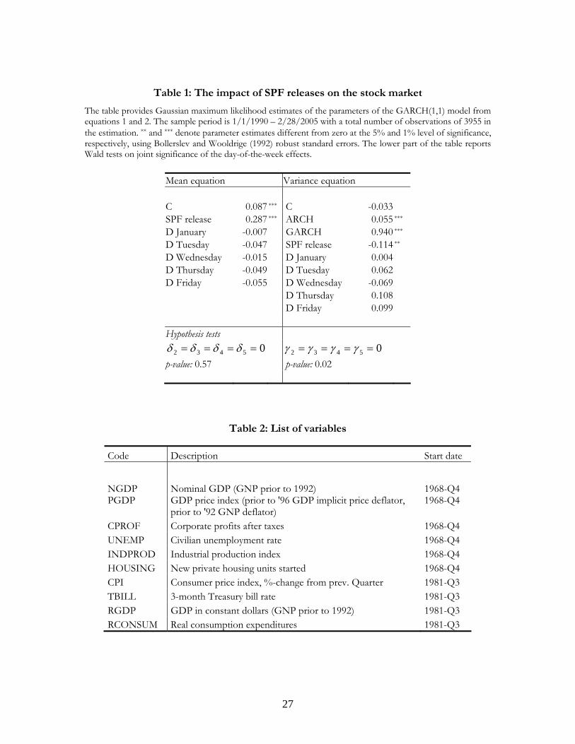
Table 1: The impact of SPF releases on the stock market
The table provides Gaussian maximum likelihood estimates of the parameters of the GARCH(1,1) model from equations 1 and 2. The sample period is 1/1/1990 – 2/28/2005 with a total number of observations of 3955 in the estimation. ** and *** denote parameter estimates different from zero at the 5% and 1% level of significance, respectively, using Bollerslev and Wooldrige (1992) robust standard errors. The lower part of the table reports Wald tests on joint significance of the day-of-the-week effects.
Mean equation Variance equation C 0.087 *** C -0.033 SPF release 0.287 *** ARCH 0.055 ***
D January -0.007 GARCH 0.940 ***
D Tuesday -0.047 SPF release -0.114 **
D Wednesday -0.015 D January 0.004 D Thursday -0.049 D Tuesday 0.062 D Friday -0.055 D Wednesday -0.069 D Thursday 0.108 D Friday 0.099 Hypothesis tests
05432 ==== δδδδ 05432 = γ = γ = γ =γ p-value: 0.57 p-value: 0.02
Table 2: List of variables
Code Description Start date
NGDP Nominal GDP (GNP prior to 1992) 1968-Q4 PGDP
GDP price index (prior to '96 GDP implicit price deflator, prior to '92 GNP deflator)
1968-Q4
CPROF Corporate profits after taxes 1968-Q4 UNEMP Civilian unemployment rate 1968-Q4 INDPROD Industrial production index 1968-Q4 HOUSING New private housing units started 1968-Q4 CPI Consumer price index, %-change from prev. Quarter 1981-Q3 TBILL 3-month Treasury bill rate 1981-Q3 RGDP GDP in constant dollars (GNP prior to 1992) 1981-Q3 RCONSUM Real consumption expenditures 1981-Q3
27

28
ttYt NBER εβασ ++= * Y
tσPanel A shows betas and Newey and West (1987) corrected t-values for β in the regression
, where is either macroeconomic uncertainty (U1) or macroeconomic volatility (V1) and NBER is a dummy variable with value one if the economy is in a recession and zero otherwise. Panel B provides correlations between macroeconomic uncertainty and macroeconomic volatility. The upper triangle of panel C holds the correlation matrix for the uncertainty series, the lower triangle holds the correlation matrix for the volatility series. Bold numbers indicate significantly different from zero at the 5%-level of significance at least. All findings are for the period 1969-2004.
Table 3: Relationships between uncertainty, volatility and recessions
NGDP PGDP CPROF UNEMP INDPROD HOUSING PANEL A β(U1) 0.32 0.26 1.51 0.12 0.49 3.34 t-value 2.61 3.23 2.74 5.63 3.98 3.67
β(V1) 0.45 0.41 0.09 1.00 0.78 0.55 t-value 1.53 1.78 0.30 4.87 4.64 1.85 PANEL B ρ(U1,V1) 0.24 0.12 0.00 0.40 0.39 0.30 PANEL C NGDP -- 0.58 0.36 0.67 0.67 0.68
PGDP 0.01 -- 0.30 0.49 0.55 0.53
CPROF 0.15 0.05 -- 0.42 0.43 0.43
UNEMP 0.01 0.18 0.07 -- 0.75 0.70
INDPROD 0.30 0.06 0.10 0.28 -- 0.71
HOUSING 0.01 0.05 0.07 0.02 0.19 --

Table 4: Stock market volatility and macroeconomic uncertainty and volatility: before 1997
The regression modelt
YttSP εβσασ ++=,500
contains a constant (not shown in the table) and various measures of macroeconomic uncertainty and volatility (U1, U4, V1
and V4). For each of the four sets of results, the table displays the beta-coefficient, its Newey and West (1987) t-value and the R-squared of the regression. *, ** and *** indicate parameter estimates significantly different from zero at the 10%-, 5% and 1%-level of significance, respectively. LR-long and LR-short are likelihood ratio values to test whether all macroeconomic variables (uncertainty or volatility) are redundant for the period 1969Q1–1996Q4 and 1981Q3-1996Q4, respectively. Critical values for the coefficients (parametric) as well as for the likelihood ratio redundancy tests (parametric) are based on the bootstrap experiment described in the main text with 10,000 replications.
1969Q1 – 1996Q4 1981Q3 – 1996Q4 NGDP PGDP CPROF UNEMP INDPROD HOUSING CPI TBILL RGDP RCONSUM U1 1.71 2.08 0.58 9.42 1.49 0.27 1.55 1.89 2.82 2.25 t-value 2.72 ** 1.96 * 4.37 *** 4.03 *** 4.07 *** 3.74 *** 2.56 * 1.99 3.13 ** 3.17 **
R-square 0.09 ** 0.08 ** 0.25 *** 0.16 *** 0.11 ** 0.12 ** 0.14 * 0.09 0.17 ** 0.16 **
LR-long 38.84 *** LR-short 18.66 V1 -0.02 0.23 0.02 0.52 0.41 0.31 0.33 0.42 0.44 0.56 t-value -0.09 1.36 0.14 3.17 *** 2.21 ** 2.14 * 2.38 ** 1.50 2.31 ** 2.36 *
R-square 0.00 0.02 0.00 0.08 *** 0.05 ** 0.03 * 0.06 * 0.05 * 0.06 ** 0.08 **
LR-long 15.15 ** LR-short 14.47 *** U4 0.84 0.68 0.26 5.22 0.61 0.14 1.03 1.23 1.75 0.69 t-value 3.00 ** 1.45 3.49 *** 2.97 ** 2.25 * 3.51 ** 2.09 2.04 3.24 ** 2.32 **
R-square 0.09 ** 0.06 ** 0.11 *** 0.14 ** 0.07 ** 0.13 ** 0.06 0.06 0.16 ** 0.08 **
LR-long 23.90 * LR-short 11.84 V4 0.51 0.10 0.83 0.94 0.76 1.21 1.26 0.30 0.99 1.44 t-value 0.93 0.12 1.88 3.23 ** 2.01 2.63 ** 3.52 ** 0.51 2.73 * 2.78 *
R-square 0.02 0.00 0.04 0.08 ** 0.04 0.06 * 0.19 ** 0.01 0.09 0.13 *
LR-long 13.10 LR-short 21.34 *

Table 5: Stock market volatility and macroeconomic uncertainty and volatility: from 1997
The regression modelt
YttSP εβσασ ++=,500
contains a constant (not shown in the table) and various measures of macroeconomic uncertainty and volatility (U1, U4, V1 and V4). For each of the four sets of results, the table displays the beta-coefficient, its Newey and West (1987) t-value and the R-squared of the regression. * and ** indicate parameter estimates significantly different from zero at the 10%- and 5%-level of significance, respectively. LR are likelihood ratio values on the test that all macroeconomic variables (uncertainty or volatility) are redundant for the period 1997Q1–2004Q4. Critical values for the coefficients (parametric) as well as for the likelihood ratio redundancy tests (parametric) are based on the bootstrap experiment described in the main text with 10,000 replications.
1997Q1 – 2004Q4 NGDP PGDP CPROF UNEMP INDPROD HOUSING CPI TBILL RGDP RCONSUM U1 3.92 5.88 -0.19 8.49 1.00 -2.55 -4.44 -4.91 6.09 1.93 t-value 0.87 0.91 -0.59 0.82 0.62 -2.21 * -2.59 * -0.83 1.05 0.36 R-square 0.02 0.02 0.02 0.02 0.01 0.17 ** 0.10 0.02 0.04 0.00 LR-long 13.61 V1 0.53 -0.34 0.32 0.02 -0.07 -0.01 -0.74 0.34 0.45 -0.60 t-value 0.98 -0.72 1.03 0.03 -0.15 -0.03 -1.27 1.80 1.74 -1.97 R-square 0.02 0.02 0.02 0.00 0.00 0.00 0.04 0.02 0.05 0.06 LR-long 9.97 U4 1.29 -1.21 -0.11 16.27 0.82 -0.60 -7.46 -3.69 5.47 4.25 t-value 0.73 -0.26 -0.42 1.44 0.49 -0.82 -2.50 * -0.92 2.58 * 1.02 R-square 0.02 0.00 0.02 0.07 0.01 0.03 0.12 0.03 0.11 * 0.05 LR-long 14.36 V4 2.47 -2.21 -0.43 0.35 0.39 0.13 -2.21 0.68 0.14 0.79 t-value 2.37 -1.31 -0.37 0.38 0.41 0.11 -1.83 1.59 0.07 0.65 R-square 0.10 0.10 0.00 0.00 0.00 0.00 0.13 0.04 0.00 0.01 LR-long 19.93
30

Table 6: Incremental effects
The regression modelttSP
YttSP εγσβσασ +++= −1,500,500
contains a constant, lagged stock market volatility (both not shown in the table) and various measures of macroeconomic uncertainty and volatility (U1, U4, V1 and V4). For each of the four sets of results, the table displays the beta-coefficient, its Newey and West (1987) t-value and the R-square of the regression. *, ** and *** indicate significantly different from zero at the 10%-, 5%- and 1%-level of significance, respectively. Significance levels are based on bootstrapped critical values (parametric) with 10,000 replications.
1969Q1 – 1996Q4 1981Q3 – 1996Q4 NGDP PGDP CPROF UNEMP INDPROD HOUSING CPI TBILL RGDP RCONSUM U1 0.86 1.14 0.36 4.05 0.49 0.10 0.78 1.25 1.51 1.37 t-value 2.49 ** 1.48 3.06 *** 2.10 * 1.44 1.52 2.17 * 1.88 2.65 ** 3.69 ***
R-square 0.37 0.37 0.43 0.37 0.36 0.36 0.42 0.43 0.44 0.45 V1 -0.15 0.13 0.06 0.28 0.16 0.14 0.23 0.18 0.20 0.26 t-value -1.04 1.45 0.81 2.87 ** 1.25 0.91 1.94 * 0.76 1.41 1.50 R-square 0.35 0.35 0.35 0.37 0.35 0.35 0.42 0.40 0.41 0.41 U4 0.45 0.40 0.16 2.72 0.14 0.05 0.37 0.88 1.13 0.44 t-value 2.28 ** 1.20 2.03 * 2.79 ** 0.75 1.41 1.28 2.23 * 3.83 *** 2.36 **
R-square 0.38 0.37 0.39 0.39 0.36 0.37 0.40 0.42 0.46 0.42 V4 0.20 -0.10 0.33 0.27 0.07 0.36 0.72 0.01 0.39 0.55 t-value 0.60 -0.28 1.06 1.20 0.30 1.30 2.80 ** 0.04 1.34 1.70 R-square 0.35 0.35 0.35 0.35 0.35 0.35 0.45 0.39 0.41 0.41
31

Table 7: Incremental and additional effects
Panel A reports beta-coefficients and Newey and West (1987) t-values for the regression model t
volYtvol
uncertYtuncerttSP εσβσβασ +++= ,
.,
.,500 with for each macroeconomic
variable both uncertainty and volatility included (U1 & V1 and U4 & V4). Panel B gives beta coefficients, Newey and West (1987) corrected t-values of the regression ttSP
volYtvol
uncertYtuncerttSP εγσσβσβασ ++++= −1,500
,.
,.,500
where lagged stock market volatility is included as additional regressor. *, ** and *** indicate significantly different from zero at the 10%-, 5%- and 1%-level of significance, respectively. Significance levels are based on bootstrapped critical values (parametric) with 10,000 replications. The constant and lagged stock market volatility are not shown in the table.
1969Q1 – 1996Q4 1981Q3 – 1996Q4 NGDP PGDP CPROF UNEMP INDPROD HOUSING CPI TBILL RGDP RCONSUMPANEL A U1 1.83 2.05 0.59 8.10 1.30 0.26 1.38 1.56 2.58 2.06 t-value 2.67 ** 2.00 * 4.35 *** 2.95 ** 3.59 *** 3.43 ** 2.02 1.60 2.97 ** 2.96 **
V1 -0.15 0.22 -0.04 0.24 0.20 0.18 0.12 0.18 0.31 0.46 t-value -0.78 1.38 -0.40 1.55 1.24 1.18 0.88 0.66 1.76 2.11 *
U4 1.00 0.70 0.24 4.35 0.50 0.13 -0.03 1.62 1.47 0.57 t-value 2.86 ** 1.44 2.73 ** 2.52 * 1.59 3.06 ** -0.07 1.68 2.22 * 2.05 *
V4 -0.35 -0.22 0.36 0.56 0.38 0.23 1.28 -0.33 0.36 1.29 t-value -0.58 -0.35 0.83 1.73 0.95 0.60 3.11 ** -0.39 0.75 2.56 PANEL B U1 1.02 1.14 0.36 3.05 0.40 0.09 0.57 1.28 1.42 1.31 t-value 2.49 ** 1.49 2.99 *** 1.30 0.98 1.30 1.33 1.73 2.57 ** 3.11 **
V1 -0.22 0.13 0.02 0.19 0.11 0.10 0.15 -0.02 0.16 0.23 t-value -1.43 1.42 0.24 1.56 0.72 0.63 1.10 -0.06 1.06 1.31 U4 0.57 0.43 0.15 2.55 0.15 0.05 -0.23 1.56 1.20 0.42 t-value 2.15 * 1.22 1.68 2.55 ** 0.67 1.20 -0.60 2.83 ** 3.35 *** 2.33 **
V4 -0.27 -0.38 0.16 0.14 -0.01 0.01 0.80 -0.59 -0.10 0.48 t-value -0.65 -1.22 0.53 0.60 -0.05 0.03 2.55 ** -1.46 -0.29 1.44
32

Table 8: Forecasting stock market volatility
Panel A (B) reports beta-coefficients and Newey and West (1987) t-values for the regression model )1,(),1(,500
,1.
,1.)1,(,500 +−−−+ ++++= ttttSP
volYtvol
uncertYtuncertttSP εγσσβσβασ with
for each macroeconomic variable both U1 uncertainty (U4) and V1 volatility (V4) included. *, ** and *** indicate significantly different from zero at the 10%-, 5%- and 1%-level of significance, respectively. Significance levels are based on bootstrapped critical values (parametric) with 10,000 replications. The constant and lagged stock market volatility are not shown in the table.
1969Q2 – 1996Q4 1981Q3 – 1996Q4 NGDP PGDP CPROF UNEMP INDPROD HOUSING CPI TBILL RGDP RCONSUMPANEL A U1 0.85 1.85 0.22 2.60 0.77 0.04 1.46 1.36 -0.04 1.21 t-value 2.49 ** 2.35 ** 1.76 1.11 1.91 * 0.81 4.30 *** 1.83 -0.06 1.71 V1 -0.11 -0.11 -0.07 -0.09 -0.17 0.10 0.02 -0.12 -0.09 -0.15 t-value -0.71 -0.78 -0.72 -0.56 -1.22 0.72 0.13 -0.53 -0.35 -0.80 PANEL B U4 0.59 0.56 0.05 2.20 0.40 0.04 0.67 1.53 0.76 0.00 t-value 2.53 ** 2.09 * 0.67 1.83 1.87 * 1.04 1.68 2.68 ** 1.58 0.02 V4 -0.25 -0.62 0.12 -0.21 -0.31 -0.08 0.48 -0.58 -0.03 0.37 t-value -0.49 -1.44 0.30 -0.81 -0.91 -0.20 1.21 -1.35 -0.07 0.91
33

8 YMP Your Leadership Development Program
�����������������������
�����������������������
�����������������������
�����������������������
Nyenrode Business UniversiteitNyenrode Research Group
Straatweg 25Postbus 130, 3620 AC BREUKELEN
t +31 346 291 696f +31 346 291 250e [email protected] www.nyenrode.nl/nrg