RELIABILITY EVALUATION OF ELECTRIC POWER GENERATION

SYSTEMS WITH SOLAR POWER

A Thesis

by

SAEED SAMADI

Submitted to the Office of Graduate and Professional Studies of Texas A&M University

in partial fulfillment of the requirements for the degree of

MASTER OF SCIENCE

Chair of Committee, Chanan Singh

Committee Members, Garng Huang Alex Sprintson Sergiy Butenko Head of Department, Chanan Singh

December 2013

Major Subject: Electrical Engineering

Copyright 2013 Saeed Samadi

ii

ABSTRACT

Conventional power generators are fueled by natural gas, steam, or water flow.

These generators can respond to fluctuating load by varying the fuel input that is done by

a valve control. Renewable power generators such as wind or solar, however, are not

controllable since their fuel sources are intermittent in nature. This creates difficulties for

designing generation systems having renewable sources. Therefore, a mechanism is

needed to predict their power outputs and evaluate the generation system reliability. This

information is used to calculate the reliability indices such as Loss of Load Expectation

(LOLE), frequency of capacity deficiency, and Expected Unserved Energy (EUE). These

indices help to estimate to what extent renewable power plants with intermittent sources

can substitute for other power generations in the system while maintaining the same

reliability standards. This study is used in generation planning of power systems with

intermittent sources.

The primary objective of this thesis is to study reliability evaluation of generation

systems including Photovoltaic (PV) and Concentrated Solar Power (CSP) plants. Unit

models of PV and CSP are developed first, and then generation system model is

constructed to evaluate the reliability of generation systems.

In addition to reliability indices calculations, a methodology is developed to

evaluate the capacity credit of PV and CSP plants. This is accomplished by calculating

the Effective Load Carrying Capability (ELCC) of these plants. ELCC is the extra load

that can be served after addition of the solar power plant to the conventional system. The

iii

capacity credit information, in addition to its use in generation system planning, can also

be used for cost comparison between conventional power plants and solar power plants.

The methodology developed in this thesis is applied to IEEE Reliability Test

System (IEEE-RTS) to study the system reliability for different penetration levels of

solar power and evaluate their capacity credits. It is found that generation system

reliability drops as solar power penetration level increases. Also, solar plant capacity

credit drops as its penetration level increases in generation system.

iv

DEDICATION

To my parents and grandparents for their love and support

v

ACKNOWLEDGEMENTS

I would like to thank my advisor, Dr. Chanan Singh, for his continuous

supervision and guidance throughout my research study. I would also like to thank my

committee members, Dr. Garng Huang, Dr. Alex Sprintson, Dr. Sergiy Butenko, and Dr.

Guy Curry, for their support.

Thanks also go to my friends and colleagues for their encouragement and the

department faculty and staff for making my time at Texas A&M University a great

experience.

vi

NOMENCLATURE

LOLE Loss of Load Expectation

EUE Expected Unserved Energy

PV Photovoltaic

CSP Concentrated Solar Power

ELCC Effective Load Carrying Capability

NREL National Renewable Energy Laboratory

SRRL Solar Radiation Research Laboratory

BMS Base Measurement System

vii

TABLE OF CONTENTS

Page

ABSTRACT .......................................................................................................................ii DEDICATION .................................................................................................................. iv ACKNOWLEDGEMENTS ............................................................................................... v NOMENCLATURE .......................................................................................................... vi TABLE OF CONTENTS .................................................................................................vii LIST OF FIGURES ........................................................................................................... ix LIST OF TABLES ............................................................................................................. x CHAPTER I INTRODUCTION AND LITERATURE REVIEW ................................... 1

1.1 Background .............................................................................................................. 1 1.2 Literature Review ..................................................................................................... 2

1.3 Organization of Thesis ............................................................................................. 4

CHAPTER II BASIC RELIABILITY CONCEPTS ......................................................... 5

2.1 Basics ....................................................................................................................... 5 2.2 Reliability Indices .................................................................................................... 6

CHAPTER III GENERATION UNIT MODELING ....................................................... 11

3.1 Conventional Unit Modeling .................................................................................. 11 3.2 Solar Unit Overview............................................................................................... 13

3.2.1 PV Units .......................................................................................................... 13

3.2.2 CSP Units ........................................................................................................ 15 3.3 Solar Unit Modeling ............................................................................................... 17

3.3.1 PV Units .......................................................................................................... 17 3.3.2 CSP Units ........................................................................................................ 22

CHAPTER IV GENERATION SYSTEM MODELING ................................................. 24

4.1 Generation System Model Elements ...................................................................... 24

viii

4.2 Unit Addition Algorithm ........................................................................................ 25 4.3 Simplified Unit Addition Algorithm for Subsystems ............................................ 27

4.3.1 Conventional and CSP Subsystems ................................................................. 27 4.3.2 PV Subsystem .................................................................................................. 28

4.4 Impact of Solar Radiation on Solar Plants ............................................................. 32 4.4.1 PV Plants ......................................................................................................... 33 4.4.2 CSP Plants ....................................................................................................... 34

CHAPTER V RELIABILITY INDICES CALCULATION AND CAPACITY

CREDIT EVALUATION ........................................................................ 36

5.1 Load Modeling ....................................................................................................... 36 5.2 Reliability Indices Calculation ............................................................................... 37

5.2.1 LOLE ............................................................................................................... 37 5.2.2 EUE ................................................................................................................. 38 5.2.3 Frequency of Capacity Deficiency .................................................................. 41

5.3 Capacity Credit Evaluation .................................................................................... 43 CHAPTER VI CASE STUDY ......................................................................................... 45

6.1 Introduction ............................................................................................................ 45 6.2 IEEE Reliability Test System ................................................................................. 45

6.2.1 Load Model ..................................................................................................... 46 6.2.2 Generation System .......................................................................................... 48

6.3 Generation System with Solar Units ...................................................................... 49 6.3.1 Conventional Subsystem ................................................................................. 50 6.3.2 PV Subsystem .................................................................................................. 51 6.3.3 CSP Subsystem ................................................................................................ 53

6.4 Solar Radiation Effect ............................................................................................ 54 6.5 Reliability Indices Calculation ............................................................................... 55

6.5.1 Results ............................................................................................................. 55 6.5.2 Discussion ....................................................................................................... 55

6.6 Capacity Credit Evaluation .................................................................................... 56 6.6.1 Results ............................................................................................................. 56 6.6.2 Discussion ....................................................................................................... 58

CHAPTER VII CONCLUSION ...................................................................................... 59 REFERENCES ................................................................................................................. 61 APPENDIX ...................................................................................................................... 63

ix

LIST OF FIGURES

Page

Figure 1 - Generation-load model example for LOLE ....................................................... 8

Figure 2 - Generation-load model example for Freq & Duration ...................................... 9

Figure 3 - Generation-load model example for EUE ......................................................... 9

Figure 4 - 2-state unit model of a conventional generator ............................................... 11

Figure 5 - Utility scale PV unit configuration .................................................................. 14

Figure 6 - CSP plant configuration [10] ........................................................................... 15

Figure 7 - State transition diagram for an n-inverter system ............................................ 19

Figure 8 - State transition diagram for 10-inverter & transformer PV unit ..................... 21

Figure 9 - Capacity credit evaluation method .................................................................. 44

x

LIST OF TABLES

Page

Table 1 - State probabilities for 10-inverter system ......................................................... 20

Table 2 - Frequency calculations for 10-inverter system ................................................. 20

Table 3 - Frequency calculations for 10-inverter & transformer PV unit ........................ 22

Table 4 - Generation system model .................................................................................. 24

Table 5 - Existing generation system model .................................................................... 25

Table 6 - Capacity outage levels of the unit being added ................................................ 25

Table 7 - Capacity outage levels after unit addition ......................................................... 26

Table 8 - Capacity outage levels after 2-state unit addition ............................................. 28

Table 9 - Capacity outage levels after n-state unit addition ............................................. 29

Table 10 - Capacity outage levels and state probabilities of an 11-state PV unit ............ 30

Table 11 - State transition frequency of an 11-state PV unit ........................................... 30

Table 12 - Addition of an 11-state unit to 21-state generation system ............................ 32

Table 13 - Generation system model of solar plants ........................................................ 35

Table 14 - Weakly peak load in percent of annual peak .................................................. 46

Table 15 - Daily peak load in percent of weekly peak ..................................................... 47

Table 16 - Hourly peak load in percent of daily peak ...................................................... 47

Table 17 - Base system generation units .......................................................................... 48

Table 18 - Generation system model of the conventional subsystem .............................. 49

Table 19 - Solar power capacity used for different penetration levels ............................. 49

xi

Table 20 - Generation system model of the conventional subsystem for 5% solar penetration ....................................................................................................... 50

Table 21 - Generation system model of the conventional subsystem for 20% solar

penetration ....................................................................................................... 50 Table 22 - PV unit reliability data .................................................................................... 51

Table 23 - PV unit capacity outage levels ........................................................................ 51

Table 24 - Number of PV units for different penetration levels ...................................... 52

Table 25 - Generation system model of the PV subsystem for 5% solar penetration ...... 52

Table 26 - Generation system model of the PV subsystem for 20% solar penetration .... 52

Table 27 - CSP unit reliability data .................................................................................. 53

Table 28 - Generation system model of the CSP subsystem for 5% solar penetration .... 53

Table 29 - Generation system model of the CSP subsystem for 20% solar penetration .. 53

Table 30 - Reliability indices calculation ......................................................................... 55

Table 31 - LOLE before and after adding solar units for 5% penetration........................ 56

Table 32 - Peak load increase for capacity credit evaluation ........................................... 56

Table 33 - LOLE before and after adding solar units for 20% penetration...................... 57

Table 34 - Peak load increase for capacity credit evaluation ........................................... 57

1

CHAPTER I

INTRODUCTION AND LITERATURE REVIEW

1.1 Background

Sources of renewable energy have become increasingly popular in recent years

due to environmental concerns resulting from fossil fuel consumption in conventional

power plants. The conventional power generators are mainly gas turbines and steam

turbines. This generation mix is changing with the rapid growth in the number of

renewable power plants such as solar and wind. As of today, the percentage of

renewable power generation is small in the generation mix, but all indications are that it

is increasing rapidly. However, the increase in penetration level of renewable power

introduces its own challenges. The key challenge is the intermittency of renewable

power and difficulty in its predictability [1]. Renewable power plants generate power

when the fuel source is available. Therefore, they are not dispatchable like the traditional

power plants [2]. These difficulties contribute to operational challenges of power

systems with high integration of renewable sources. There are issues in power system

planning, scheduling, frequency regulations, and stability [1]. These challenges have led

to view renewable power plants as energy sources, rather than power sources [2]. But,

since in power system operation, power availability is more critical than energy

availability in meeting the load, it is important to evaluate the power capacity value, also

known as capacity credit, of these plants. All of these issues are subjects of ongoing

2

research. These studies are trying to improve the existing methodology or come up with

new solutions to tackle these issues.

This thesis develops a methodology for quantitative reliability study of

generation systems with solar power and to evaluate the capacity credit of solar power

plants. This methodology assists power system planners in designing generation systems

with renewable power, in particular solar power, which meets the required reliability

standards.

1.2 Literature Review

Extensive research has been done to deal with operational challenges of

renewable power. Since wind technology is more mature than solar, most of available

literature focuses on wind power. However, one can expect similar challenges and

solutions in solar power.

There are many papers that deal with unpredictability of renewable sources.

These studies use historical weather and load data to predict the power generation and

load on hourly basis. The correlation between generation and load needs to be

considered. Ref. [3] addresses a probabilistic study of wind electric conversion systems

from the point of view of reliability and capacity credit. It models wind generators as

multistate units. This paper does not consider the correlation between generation and

load. It also does not take into account the failure characteristic of wind generators. Ref.

[4] develops a methodology for photovoltaic system reliability and economic analysis.

This methodology is based on load reduction approach. This paper also does not take

3

into account the failure characteristics of photovoltaic system. Ref. [5] studies reliability

modeling of generation systems including unconventional energy sources. It considers

two unconventional sources: wind and photovoltaic power plants. This paper calculates

the loss of load expectation (LOLE) and frequency of capacity deficiency on hourly

basis for the generation system. It does not, however, calculate the expected unserved

energy (EUE). Ref. [6] develops an efficient technique for reliability analysis of power

systems including time dependent sources. It uses the clustering technique to calculate

the LOLE and EUE. This paper does not address frequency calculations. Ref. [7]

develops a method for calculating expected unserved energy in generating system

reliability analysis. It introduces the concept of expected value or mean value of capacity

outage. This is used to calculate the LOLE and EUE on hourly basis, but in a more

efficient way than ref. [5]. It does not, however, calculate the frequency of capacity

deficiency. Ref. [8] studies reliability evaluation of grid-connected photovoltaic power

systems. It analyses component failures in utility scale PV power system, but it does not

address the reliability impact of PV on the overall generation system.

There are a number of papers that study capacity credit of wind power plants.

Ref. [9] evaluates current methods to calculate capacity credit of wind power. A

chronological reliability method and a probabilistic reliability method to calculate the

capacity credit is explained. Ref. [10] calculates capacity value of wind power using the

LOLE and effective load carrying capability (ELCC) indices, iteratively. These

approaches can also be used to evaluate capacity credit of solar power plants.

4

1.3 Organization of Thesis

Chapter II introduces basic concepts of generation system reliability. Reliability

modeling of generation units is formulated in Chapter III. The configuration of large

scale PV and CSP plants is studied. This configuration is important factor in reliability

studies. Generation system model for each subsystem is developed in Chapter IV.

Chapter V formulates methodologies for calculating the reliability indices such as

LOLE, Frequency of capacity deficiency, and EUE of the composite generation system.

In addition, this chapter introduces methods to evaluate capacity credit of solar power

plants. Chapter VI provides a case study for reliability evaluation of generation systems

with solar power. The IEEE Reliability Test System is used for this case study. Finally,

Chapter VII draws a conclusion about the methodologies developed and the case study

results.

5

CHAPTER II

BASIC RELIABILITY CONCEPTS

2.1 Basics

System reliability is defined as the probability that the system will perform its

intended function for a given period of time under stated environmental conditions [11].

Electric power system reliability can be defined as the probability that electricity is being

delivered to customers with the required amount and quality. The objective of electric

power systems is to supply electrical energy to consumers at low cost while

simultaneously providing acceptable, or economically justifiable, service quality [11].

An electric power system is very complex and consists of many components. Therefore,

its reliability studies are performed for different subsystems. Three major areas of power

system reliability analysis are:

Generation system reliability

Transmission system reliability

Distribution system reliability.

The focus of this thesis is on generation system reliability. Generation system

reliability deals with the relative ability of the system to supply system load considering

that generation units may be out of service when needed due to planned or unplanned

outages or that the basic energy sources may be inadequate [11]. Generation system

reliability, also known as generation system adequacy, is to be contrasted with security

which deals with the relative ability of the system to survive sudden shocks or upsets

6

such as faults or equipment failures without cascading failures or loss of stability [11].

Generation system reliability is usually measured through the use of some reliability

indices which quantify system reliability performance and it is enforced through a

criterion based on an acceptable value of this reliability index [11]. Some utilities rely on

adequacy criteria whose values have been chosen based on engineering judgment to

yield a reasonable balance between system cost and reliability performance and which

have been validated by historical experience. However, if adequacy criteria are based on

probabilistic indices which bear reasonable relationships to the actual reliability

performance of the system, more pragmatic methods may be employed to determine

proper values of the criteria [11].

2.2 Reliability Indices

Reliability indices of generation system can be broadly divided into two

categories [11]:

1. Deterministic indices: These indices reflect postulated conditions. They

are not directly indicative of electrical system reliability and are not

responsive to most parameters which influence system reliability

performance. Therefore, these indices are of limited value for choosing

between planning alternatives. Their calculation is however, simple and

requires little data.

2. Probabilistic indices: These indices directly reflect the uncertainty which

is inherent in the power system reliability problem and have the capability

7

of reflecting the various parameters which can impact system reliability.

Therefore, probabilistic indices permit the quantitative evaluation of

system alternatives through direct consideration of parameters which

influence reliability. This capability accounts for the increasing popularity

and use of probabilistic indices.

There are normally two deterministic indices that are used for generation system

reliability [11]:

1. Percent reserve margin: defined as excess of installed generating capacity

over annual peak load expressed in percent of annual peak load. It

provides a reasonable relative estimate of reliability performance if

parameters other than margin remain essentially constant. It, however,

does not directly reflect system parameters such as unit size, outage rate,

and the load shape.

2. Reserve margin in terms of largest unit: this index recognizes the

importance of unit capacities in relationship to reserve margin.

There are a number of probabilistic indices that are used for generation system

reliability evaluation. Each index gives information about the expected behavior of the

system.

Let us consider Fig. 1. In this figure, the y-axis is power and the x-axis is time.

The straight line represents the load (assumed to be constant for simplicity), and the

other line represents the available generation capacity. The generation capacity can

change due to failures and repairs of the generating units.

8

Figure 1 - Generation-load model example for LOLE

In order to evaluate the reliability of the generation-load system, one desirable

index is the probability of generation capacity deficiency or loss of load probability. This

can be estimated as (t1+t2)/t.

In this example the sample size is only two and it is understood that this is not

sufficient for purposes of estimation but this simple example can be used to illustrate the

basic concepts. Alternatively, we can introduce loss of load expectation that gives us

information about the time duration that is used. The estimate is given by ((t1+t2)/t )t.

Now, let us consider the two graphs in Fig. 2. The LOLE of both graphs are the

same. However, these two graphs do not represent the same scenario. In order to

differentiate these two scenarios of generation capacity deficiency, it is required to

introduce another reliability index called frequency of capacity deficiency. The

frequency in the first graph is 1 while the frequency in the second graph is 2. In addition

to frequency, the duration of each frequency can also be considered. This is referred to

as frequency & duration index.

9

Figure 2 - Generation-load model example for Freq & Duration

Next, let us consider the two graphs in Fig. 3:

Figure 3 - Generation-load model example for EUE

They both have same LOLE and Freq & Duration. However, they are different

scenarios of generation capacity deficiency. Therefore, another reliability index needs to

10

be introduced to differentiate these scenarios. This index is called Expected Unserved

Energy (EUE). EUE calculated the total energy that was not supplied due to the

generation capacity deficiency.

These three indices, which are the main probabilistic indices for generation

system reliability evaluation, are defined below [11]:

1. Loss of Load Expectation (LOLE):

a. DLOLE is the expected number of days per year on which

insufficient generating capacity is available to serve the daily peak

load

b. HLOLE is the expected number of hours per year when

insufficient generating capacity is available to serve the load

2. Frequency and Duration of capacity shortage events (F&D):

a. Frequency of generating capacity shortage events is defined to be

the expected (average) number of such events per year

b. Duration is the expected length of capacity shortage periods when

they occur

3. Expected Unserved Energy (EUE): This index measures the expected

amount of energy which will fail to be supplied per year due to generative

capacity differences and/or shortages in basic energy supplies.

11

CHAPTER III

GENERATION UNIT MODELING

In order to evaluate reliability of generation systems, each generator must be

represented by a model. These models reflect the performance of generators in various

states. The individual generator model is referred to as unit model. Unit models indicate

various states with transition rates between them. From these transition rates, probability

of each state, and frequency of transition from one state to another state is obtained for

generating units. Unit models are combined together to obtain the generation system

model. The unit modeling of conventional and solar generators is described next.

3.1 Conventional Unit Modeling

The conventional generator can be modeled as a 2-state or a 3-state unit. If

modeled as a 2-state unit, they have up-state where the unit is fully available and down-

state where the unit is on forced outage. On the other hand, if modeled as a 3-state unit,

there is a third state in which the unit is said to be derated. In this case, the unit is

operating below the rated capacity because of partial failure. In this thesis, the

conventional generator is modeled as a 2-state unit, which is shown in Fig. 4.

Figure 4 - 2-state unit model of a conventional generator

12

The transition rate from up-state to down-state is called failure rate and is

represented by λ, and the transition rate from down-state to up-state is called repair rate

and is represented by µ. Frequency of encountering state j from state i is the expected

number of transition from state i to state j per unit time. The frequency of transition from

one state to another state is calculated based on frequency balance approach. The

frequency balance concept states that in steady state, frequency of encountering a state

equals the frequency of exiting from that state [11]. The state probabilities and the

transition frequency in a 2-state unit are calculated as:

where

λ is the failure rate of the generator

μ is the repair rate of the generator

is the frequency of transition from state i to state j.

In a 2-state unit with rated capacity of C, when the unit is in up-state, the

available capacity is C and the capacity outage level is 0. On the other hand, when the

unit is in down state, the available capacity is 0 and the capacity outage level is C.

13

3.2 Solar Unit Overview

There are two types of solar generators considered in this thesis. These are

photovoltaic (PV) generators and concentrated solar power (CSP) generators. A brief

introduction about PV and CSP units and their principle of power generation is given

before modeling these units.

3.2.1 PV Units

PV plants generate power by converting the solar radiations into electricity. The

solar radiation conversion into electricity is accomplished in photovoltaic cells. In order

to increase the generated voltage and current, these cells are connected in series-parallel

combinations. A number of PV cells connected in series form a PV panel or a PV

module. These modules are building blocks of a PV system. PV systems are used either

as a stand-alone system in which case it consists of few modules or as a grid-connected

unit in which case it consists of several thousands of modules. These grid-connected PV

units are called utility scale PV plants and are typically greater than 1 MW in size. In a

utility scale PV plant, modules are interconnected in certain configurations. A number of

PV modules connected in series form a string and a number of strings in parallel form an

array. Therefore, an array is a series-parallel combination of PV modules to achieve a

desired voltage and current level. These arrays are connected to a central inverter. In a

utility scale PV plant there are a number of central inverters depending on the number of

arrays and plant rating. In this thesis, since large scale solar power plant is intended,

utility scale PV plant is considered for reliability evaluation. There are various

14

configurations for large scale PV units. Fig. 5 shows a typical configuration of a utility

scale PV unit [8].

Some PV plants have tracking system to follow the solar radiation and increase

the plant energy output. This, however, increases the plant investment cost. For utility

scale PV plant, this increased cost is usually more than the gained output, and so most of

the utility scale PV plants do not have tracking system. The PV panels are tilted in a

certain angle to maximize radiation absorption. The tilt angle is proportional to latitude

of the plant location.

Figure 5 - Utility scale PV unit configuration

15

3.2.2 CSP Units

CSP plants generate power by concentrating sunlight to generate heat and

convert that heat into electrical power in thermal plants. The solar heat is concentrated

into a point using reflecting mirrors to produce high temperature. This temperature is

used to absorb heat by a working fluid. Typically, molten salt is used for this purpose

due to its heat transfer and thermal storage capabilities. This fluid is moved to a high

temperature tank from where it is taken to boiler for steam production. After producing

steam, the fluid is moved to a low temperature tank and then goes back to the solar field.

The steam is used to produce electricity in the conventional steam turbines. These

processes are shown in Fig. 6.

Figure 6 - CSP plant configuration [12]

With significant drop in PV modules manufacturing cost in recent years, CSP

plants are less attractive economically; however, they have an advantage over PV plants

from system operation point of view. A desirable feature in CSP plant is the ability to

16

store the thermal energy. This is done in the high temperature tank. The duration of this

storage depends on the working fluid and the tank, which can be from several hours up

to few days [13][14]. This makes CSP plants to be dispatchable as long as thermal

storage is available. Consequently, the CSP plants are called partially dispatchable

generators. Even in the absence of storage, unlike PV plants, the CSP plant output does

not drop immediately due to thermal inertia [13][14].

Since CSP plants concentrate the solar radiation to generate heat, they must have

a sun tracking system. Otherwise, the plant efficiency drops significantly. There are

different types of CSP technologies. These technologies differ in means to concentrate

the sunlight:

Parabolic trough: this technology uses linear parabolic trough as a

reflector to concentrate the sunlight. A receiver consisting of a tube

positioned along the focal line of the reflectors. The working fluid flows

through this tube to absorb the heat. The reflectors have a single-axis

tracking system to reflect the sun to the focal line during daylight. The

parabolic trough technology is more dominant for large CSP plants due to

its lower cost [15].

Dish engine: this technology uses parabolic dish of mirrors as a reflector

to concentrate the sunlight. This sunlight is focused into the power

conversion unit located at the focal point of the dish. The reflector has a

two-axis tracking system to reflect the sun to the focal point during

daylight. The power conversion unit consists of the thermal receiver and

17

the engine or generator. The receiver absorbs the heat and transfers it to

the engine that produces electricity. The most common type of engine

used is the Stirling engine. The dish engine system produces relative

small amounts of electricity compared to other CSP technologies (3-25

kW) [15].

Concentrating linear Frensel reflector: this technology uses linear flat or

slightly curved mirrors as a reflector to concentrate the sunlight. The

receiver tubes are fixed in space above the mirrors. The reflector mirrors

are mounted on trackers on the ground [15].

Solar power tower: this technology uses large flat mirrors as a reflector to

concentrate the sunlight. The receiver is located at the top of a tall tower.

The reflector mirrors are mounted on a two-axis tracking system [15].

3.3 Solar Unit Modeling

After understanding the basic principle of operation of solar units, it is needed to

model each unit to be used for reliability studies. This model is developed for PV and

CSP units in subsequent sections.

3.3.1 PV Units

A typical grid-connected utility scale PV unit consists of PV modules, inverters,

and transformers as it was shown in Fig. 5.

There are a number of ways in which a PV plant can fail:

18

Failure in PV modules or cells

Failure in inverters

Failure in the transformer.

There are other components, such as DC links and AC buses, in a PV plant that

can also fail, but due to low probability of failure and redundancy, their failures are not

considered. In case of failure in modules or cells, the array is still producing power, but

less than its rated value. Since number of failed cells or panels is small compared to

available ones, its impact on overall PV plant availability is minor. Consequently, the

module or cell failure is not considered in PV unit modeling.

Therefore, a PV unit failure is mainly due to failure in inverters or the

transformer. Consequently, for the PV unit model the number of states depends on the

number of inverters, where number of inverters depends on the plant size. For a PV unit

with n inverters each rated m MW, the unit rating is n×m MW. The number of states in

this case is n+1.

The same 2-state model that was used for a conventional generator is also used

for inverters with λI and µI being inverter’s failure and repair rate. The probability of up-

and down-states of the inverter is pIup and pIdown, respectively. Since the inverters are

independent of each other, i.e. there is no common mode failure, the transition can only

occur from one state to another adjacent state. The state transition diagram for an n-

inverter system is shown in Fig. 7.

19

Figure 7 - State transition diagram for an n-inverter system

The probability of each state depends on the number of inverters. In order to

explain the state probability calculations, let’s assume that there are 10 inverters (n=10)

and each inverter is rated at 1 MW (m=1). In this case, there are 11 states and probability

of each state needs to be calculated. Each state probability depends on the number of

scenarios in which that state can occur. For example, the first state (all inverters up) has

only one scenario. The second state (only one inverter down) has 10 scenarios namely

inverter 1 down, inverter 2 down, …, inverter 10 down. The number of scenarios and

state probabilities for 10-inverter case is shown in Table 1.

The frequency of transition from one state to another state is calculated based on

frequency balance approach. The frequency calculations are given in Table 2.

20

Table 1 - State probabilities for 10-inverter system

i Capacity Outage Levels (MW) No. of Scenarios State Probability (pIi) 1 0 1 (pIup)10

2 1 10 10×(pIup)9 (pIdown) 3 2 45 45×(pIup)8 (pIdown)2

4 3 120 120×(pIup)7 (pIdown)3 5 4 210 210×(pIup)6 (pIdown)4 6 5 252 252×(pIup)5 (pIdown)5 7 6 210 210×(pIup)4 (pIdown)6 8 7 120 120×(pIup)3 (pIdown)7 9 8 45 45×(pIup)2 (pIdown)8 10 9 10 10×(pIup) (pIdown)9 11 10 1 (pIdown)10

Table 2 - Frequency calculations for 10-inverter system

Transition Frequency f12 = f21 = pI2 × µI f23 = f32 = pI3 × 2µI f34 = f43 = pI4 × 3µI f45 = f54 = pI5 × 4µI f56 = f65 = pI6 × 5µI f67 = f76 = pI7 × 6µI f78 = f87 = pI8 × 7µI f89 = f98 = pI9 × 8µI

f9,10 = f10,9 = pI10 × 9µI f10,11 = f11,10 = pI11 × 10µI

Next, we must include the effect of transformer on the inverter state transition

diagram. The same 2-state model that was used for a conventional generator is also used

for a transformer with λT and µT being transformer’s failure and repair rates. The

probability of up- and down-states of the transformer is pTup and pTdown, respectively.

The state transition diagram for 10-inverter with transformer PV unit and the state

probability calculations are shown in Fig. 8.

21

0

10

State Diagram

11

5

3

2

1

4

6

7

8

9

10

µT

µT

µT

µT

µT

µT

µT

µT

µT

µT

µT λT

λT

4µI

5λI 6µI

6λI 5µI

7λI

8λI 3µI

9λI 2µI

3λI 8µI

7µI 4λI

9µI 2λI

λI 10µ

I

10λI µI 10 Iup , Tup

9 Iup, 1 Idn Tup

Tdn 10 Idn , Tup

7 Iup, 3 Idn Tup

3 Iup, 7 Idn Tup

8 Iup, 2 Idn Tup

4 Iup, 6 Idn Tup

5 Iup, 5 Idn Tup

6 Iup, 4 Idn Tup

2 Iup, 8 Idn Tup

1 Iup, 9 Idn Tup

4

2

1

3

Capacity Outage

pI1 × pTup

State Probability

5

6

7

8

9

pI2 × pTup

pI3 × pTup

pI4 × pTup

pI5 × pTup

pI6 × pTup

pI8 × pTup

pI7 × pTup

pI9 × pTup

pI10 × pTup

pI11 × pTup + pTdn

Figure 8 - State transition diagram for 10-inverter & transformer PV unit

22

Transformer failure causes full capacity outage. Therefore, a transformer down-

state is added to the last state corresponding to the full capacity outage. All other

capacity outage levels are achieved if the transformer is in up-state. So the state

probabilities are multiplied by the transformer up-state probability.

For the frequency calculations, in addition to transition from one state to

another adjacent state, there can also be transition from any state to the last state and vice

versa. This happens when the transformer is failed or repaired. The frequency

calculations are given in Table 3.

Table 3 - Frequency calculations for 10-inverter & transformer PV unit

Transition Frequency (Due to Inverter)

Transition Frequency (Due to Transformer)

f12 = f21 = pI2 × pTup × µI f1,11 = f11,1 = pI1 × pTdown × µT f23 = f32 = pI3 × pTup × 2µI f2,11 = f11,2 = pI2 × pTdown × µT f34 = f43 = pI4 × pTup × 3µI f3,11 = f11,3 = pI3 × pTdown × µT f45 = f54 = pI5 × pTup × 4µI f4,11 = f11,4 = pI4 × pTdown × µT f56 = f65 = pI6 × pTup × 5µI f5,11 = f11,5 = pI5 × pTdown × µT f67 = f76 = pI7 × pTup × 6µI f6,11 = f11,6 = pI6 × pTdown × µT f78 = f87 = pI8 × pTup × 7µI f7,11 = f11,7 = pI7 × pTdown × µT f89 = f98 = pI9 × pTup × 8µI f8,11 = f11,8 = pI8 × pTdown × µT

f9,10 = f10,9 = pI10 × pTup × 9µI f9,11 = f11,9 = pI9 × pTdown × µT fI10,11 = fI11,10 = pI11 × pTup × 10µI fT10,11 = fT11,10 = pI10 × pTdown × µT

3.3.2 CSP Units

There are a number of ways in which a CSP unit may experience failures:

Reflector failure

Receiver failure

Tracking system failure

23

Thermal unit failure.

A failure in reflector, receiver, or tracking system does not affect the entire

system. It only reduces the amount of heat being generated. Consequently, the reflector

and the receiver failures are not considered in CSP unit modeling.

Therefore, a CSP unit failure is mainly due to failure in the steam generator.

These generators are the same as the conventional generators and are modeled same as

the conventional units. Therefore, the 2-state unit model is also used for CSP units.

24

CHAPTER IV

GENERATION SYSTEM MODELING

Once units are modeled, these need to be combined to obtain the generation

system model for each subsystem. The generation system model for each subsystem has

several states. It is important to know the capacity outage level, the cumulative

probability, and the cumulative frequency of occurrence for each state.

4.1 Generation System Model Elements

Generation systems are modeled by three arrays: capacity outage levels (X),

cumulative probability of capacity outages (P), and cumulative frequency of capacity

outages (F) as follows:

Xi = one of the discrete capacity outage levels

Pi = probability of capacity outage greater than or equal to Xi

Fi = frequency of capacity outage greater than or equal to Xi.

The generation system model is arranged in a tabular form with capacity outage

levels sorted in ascending order. Table 4 indicates a generation system model in a tabular

form. Index i is the number of capacity outage level in the generation system model.

Table 4 - Generation system model

i Xi = Capacity Outage Levels Pi (Capout≥Xi) Fi (Capout≥Xi) 1 X1 P1 F1 2 X2 P2 F2 3 X3 P3 F3 … … … …

25

There are number of ways to construct the generation system model. The most

common method used is called unit addition algorithm. This algorithm is used for

embedding a unit model in the generation system model. This method is explained in the

following section.

4.2 Unit Addition Algorithm

Let’s assume that the generation system model is available in the tabular form as

Table 5. We add an n-state unit to this model. Let Yi be the capacity outage level in state

i. This is shown in Table 6.

Table 5 - Existing generation system model

i Xi = Capacity Outage Levels Pi (Capout≥Xi) Fi (Capout≥Xi) 1 X1 P1 F1 2 X2 P2 F2 3 X3 P3 F3 … … … … l Xl Pl Fl

… … … … k Xk Pk Fk … … … … j Xj Pj Fj

… … … … i Xi Pi Fi

… … … …

Table 6 - Capacity outage levels of the unit being added

i Cap outage levels of the new unit 1 Y1 2 Y2 … … n Yn

26

The addition of an n-state unit, results in n subsets of states:

S1={Xi+Y1}

S2={Xi+Y2}

…

Sn-1={Xi+Yn-1}

Sn={Xi+Yn}.

These n subsets, arranged as n columns in Table 7, have an equal number of

states and in each the capacity outages are arranged in an ascending order.

Table 7 - Capacity outage levels after unit addition

S1 S2 … Sn-1 Sn X1+Y1 X1+Y2 … X1+Yn-1 X1+Yn X2+Y1 X2+Y2 … X2+Yn-1 X2+Yn X3+Y1 X3+Y2 … X3+Yn-1 X3+Yn

… … … … … Xl+Y1 Xl+Y2 … Xl+Yn-1 Xl+Yn

… … … … … Xk+Y1 Xk+Y2 … Xk+Yn-1 Xk+Yn

… … … … … Xj+Y1 Xj+Y2 … Xj+Yn-1 Xj+Yn

… … … … … Xi+Y1 Xi+Y2 … Xi+Yn-1 Xi+Yn

… … … … …

Assuming that a capacity equal to or greater than X is defined by states equal to

and greater than i, j, …, k, l in S1, S2, …, Sn-1, Sn:

P(X) = Pi p1 + Pj p2 + … + Pk pn-1 + Pl pn

F(X) = G(X) + N(X)

where

G(X) = Fi p1 + Fj p2 + … + Fk pn-1 + Fl pn

27

N(X) = (Pj – Pi) f21 + (Pk – Pi) f31 + (Pk – Pj) f32 + … + (Pl – Pi) fk1 + (Pl – Pj) fk2

+ … + (Pl – Pk) fk(k-1)

Pi = probability of capacity outage equal to or greater than Xi

Fi = frequency of capacity outage equal to or greater than Xi.

G(X) represents the frequency due to change in the states of the existing units and

N(X) represents the frequency due to change in the states of the added unit.

4.3 Simplified Unit Addition Algorithm for Subsystems

The above algorithm is explained for general n-state case. This, however, can be

simplified for conventional and CSP subsystems since 2-state units are employed. For

PV subsystem, we still have n-state, but the state transition frequency calculations can be

simplified. These are discussed in subsequent sections.

4.3.1 Conventional and CSP Subsystems

These subsystems are composed of 2-state units. Addition of these units into

existing system will result in two subsets of states:

S1 = {Xi+Y1}

S2 = {Xi+Y2}

where Yi is the capacity outage level of a 2-state unit being added. These capacity outage

levels can be represented by Y1 = 0 and Y2 = C, where C is the capacity of the unit being

added. Therefore,

S1 = {Xi}

S2 = {Xi+C}.

28

These two subsets, arranged as two columns in Table 8, have an equal number of

states and in each the capacity outages are arranged in an ascending order.

Table 8 - Capacity outage levels after 2-state unit addition

S1 S2 X1 X1+C X2 X2+C X3 X3+C … … Xj Xj+C … … Xi Xi+C … …

Assuming that a capacity equal to or greater than X is defined by states equal to

and greater than i and j in S1 and S2:

P(X) = Pi p1 + Pj p2

F(X) = G(X) + N(X)

where

G(X) = Fi p1 + Fj p2

N(X) = (Pj – Pi) f21

Pi = probability of capacity outage equal to or greater than Xi

Fi = frequency of capacity outage equal to or greater than Xi.

4.3.2 PV Subsystem

PV units have multiple number of states, so it is required to use the original n-

state unit addition algorithm to build the generation subsystem model. However, we can

29

simplify the frequency calculations since we can only have transitions from one state to

another adjacent state or from any state to state n in case of transformer failure.

Here as before, the addition of a n-state unit, results in n subsets of states:

S1 = {Xi+Y1}

S2 = {Xi+Y2}

…

Sn-1 = {Xi+Yn-1}

Sn = {Xi+Yn}

where Yi is the capacity outage levels of a n-state unit being added.

These n subsets, arranged as n columns in Table 9, have an equal number of

states and in each the capacity outages are arranged in an ascending order.

Table 9 - Capacity outage levels after n-state unit addition

S1 S2 … Sn-1 Sn X1+Y1 X1+Y2 … X1+Yn-1 X1+Yn X2+Y1 X2+Y2 … X2+Yn-1 X2+Yn X3+Y1 X3+Y2 … X3+Yn-1 X3+Yn

… … … … … Xl+Y1 Xl+Y2 … Xl+Yn-1 Xl+Yn

… … … … … Xk+Y1 Xk+Y2 … Xk+Yn-1 Xk+Yn

… … … … … Xj+Y1 Xj+Y2 … Xj+Yn-1 Xj+Yn

… … … … … Xi+Y1 Xi+Y2 … Xi+Yn-1 Xi+Yn

… … … … …

Assuming that a capacity equal to or greater than X is defined by states equal to

and greater than i, j, …, k, l in S1, S2, …, Sn-1, Sn:

P(X) = Pi p1 + Pj p2 + … + Pk pn-1 + Pl pn

F(X) = G(X) + N(X)

30

where

G(X) = Fi p1 + Fj p2 + … + Fk pn-1 + Fl pn

N(X) = (Pj – Pi) f21 + (Pk – Pj) f32 + … + (Pl – Pk) fIn(n-1) + (Pl – Pk)( fn1 + fn2 + …

+ fTn(n-1))

Pi = probability of capacity outage equal to or greater than Xi

Fi = frequency of capacity outage equal to or greater than Xi.

Let’s assume that we want to add the 11-state PV unit that was modeled in

Chapter III to an existing generation system. The capacity outage levels and state

probabilities of this unit are given in Table 10 and the state transition frequencies are

given in Table 11.

Table 10 - Capacity outage levels and state probabilities of an 11-state PV unit

i Capacity outage levels (MW) State probabilities 1 0 p1 2 1 p2 3 2 p3 4 3 p4 5 4 p5 6 5 p6 7 6 p7 8 7 p8 9 8 p9 10 9 p10 11 10 p11

Table 11 - State transition frequency of an 11-state PV unit

Frequency (I) Frequency (T) f21 f11,1 f32 f11,2 f43 f11,3

31

Table 11 - Continued

Frequency (I) Frequency (T) f54 f11,4 f65 f11,5 f76 f11,6 f87 f11,7 f98 f11,8 f10,9 f11,9

fI11,10 fT11,10

Assume that the existing generation system has 21 states. In this case, addition of

an 11-state unit results in 11 subset of states. This is indicated in Table 12. In this case, a

capacity equal to or greater than 15 MW is defined by states equal to and greater than

16, 15, 14, …, 6 in S1, S2, …, S11:

P(15) = P16 p1 + P15 p2 + P14 p3 + P13 p4 + P12 p5 + P11 p6 + P10 p7 + P9 p8 + P8

p9 + P7 p10 + P6 p11

F(15) = G(15) + N(15)

where

G(15) = F16 p1 + F15 p2 +F14 p3 + F13 p4 + F12 p5 + F11 p6 + F10 p7 + F9 p8 + F8

p9 + F7 p10 + F6 p11

N(15) = (P15 – P16) f21 + (P14 – P15) f32 + (P13 – P14) f43 + (P12 – P13) f54 + (P11 –

P12) f65 + (P10 – P11) f76 + (P9 – P0) f87 + (P8 – P9) f98 + (P7 – P8) f10,9 + (P6 – P7)

fI11,10 + (P6 – P7) (f11,1 + f11,2 + f11,3 + f11,4 + f11,5 + f11,6 + f11,7 + f11,8 + f11,9 +

fT11,10).

The stair case in Table 12 is used to indicate the frequency of transition from

capacity outages greater than 15 MW to capacity outages less than 15 MW.

32

Table 12 - Addition of an 11-state unit to 21-state generation system

Subsets S1 S2 S3 S4 S5 S6 S7 S8 S9 S10 S11 i Cap Out (MW) 0 1 2 3 4 5 6 7 8 9 10 1 0 0 1 2 3 4 5 6 7 8 9 10 2 1 1 2 3 4 5 6 7 8 9 10 11 3 2 2 3 4 5 6 7 8 9 10 11 12 4 3 3 4 5 6 7 8 9 10 11 12 13 5 4 4 5 6 7 8 9 10 11 12 13 14 6 5 5 6 7 8 9 10 11 12 13 14 15 7 6 6 7 8 9 10 11 12 13 14 15 16 8 7 7 8 9 10 11 12 13 14 15 16 17 9 8 8 9 10 11 12 13 14 15 16 17 18 10 9 9 10 11 12 13 14 15 16 17 18 19 11 10 10 11 12 13 14 15 16 17 18 19 20 12 11 11 12 13 14 15 16 17 18 19 20 21 13 12 12 13 14 15 16 17 18 19 20 21 22 14 13 13 14 15 16 17 18 19 20 21 22 23 15 14 14 15 16 17 18 19 20 21 22 23 24 16 15 15 16 17 18 19 20 21 22 23 24 25 17 16 16 17 18 19 20 21 22 23 24 25 26 18 17 17 18 19 20 21 22 23 24 25 26 27 19 18 18 19 20 21 22 23 24 25 26 27 28 20 19 19 20 21 22 23 24 25 26 27 28 29 21 20 20 21 22 23 24 25 26 27 28 29 30

4.4 Impact of Solar Radiation on Solar Plants

Solar plant power generation depends on solar radiation. This has to be included

in the subsystem generation model. The vector containing capacity outage levels in the

PV and CSP subsystem generation model needs to be modified to include the effect of

solar radiation. The solar plant power generation, however, needs to be evaluated in

correlation with load. There is a common mistake to obtain the probability of various

power output levels of solar plants based on the solar radiation, without considering the

load. In order to consider the correlation between solar plants power level and the load,

33

the power output of these plants is evaluated on hourly basis. Therefore, the capacity

outage level vector of solar plants needs to be modified on hourly basis.

4.4.1 PV Plants

The PV plant power output directly depends on the solar radiation intensity. The

solar radiation that contributes to PV plant power generation is called global solar

radiation. Global radiation consists of direct radiation, diffuse radiation, and reflected

radiation. This radiation has to be measured at a surface perpendicular to the PV

modules.

The PV power plant rating is based on global solar radiation of 1000 W/m2. The

hourly global solar radiation in the plant location is divided by 1000 to obtain the power

output coefficient. For example, if the hourly radiation is 783 W/m2, the power output

coefficient in that hour would be 0.783. This coefficient can also be greater than one, up

to around 1.15, if the global solar radiation is greater than 1000 W/m2. The power output

coefficient, denoted by POC, is obtained hourly for the period under study:

Vector Gk is created to indicate hourly power output as follows [5]:

Gk = A × POCk

where A is the available capacity vector of the generation system model of the PV

subsystem.

34

The available capacity vector is the total plant capacity minus the capacity outage

vector:

A = C – X

where C is the total plant capacity. Therefore, the available capacity has the same

number of levels as the capacity outage.

Once Gk is obtained, the capacity outage vector X has to be modified hourly to

include the effect of fluctuating solar radiation. This is accomplished by creating a

modified capacity outage level vector X̄ for each hour of the period under study:

X̄ k = C - Gk.

4.4.2 CSP Plants

The CSP plants usually have heat storage capability. Therefore, while CSP plant

daily energy output depends on daily solar radiation, its power output is not directly

affected due to the storage capability. As a result, the methodology applied to PV plants

to obtain the power output coefficient is not applicable to CSP plants. The solar radiation

that contributes to CSP plant power generation is direct normal solar radiation. Other

radiations such as diffused or reflected do not contribute to CSP power generation. Since

CSP plants have tracking system, they can align their reflectors such that they receive

direct normal radiation during hours at which sun is available. The number of hours at

which sun is available affects CSP plant availability. Average daily radiation is

calculated to determine the average power output. This average is calculated for hours

from sunrise to sunset. The daily plant power output is considered to be constant during

35

hours of plant operation. The CSP power plant rating is based on direct normal solar

radiation of 1000 W/m2. The hourly power output coefficient for hours between sunrise

and sunset is calculated as:

From sunset to sunrise the plant output is set to be zero since no direct normal

radiation is available. Therefore, power output coefficient for hours between sunset to

sunrise is 0.

Once POCk is obtained for the period under study, the modified capacity outage

level vector X̄ can be calculated in the same manner as PV subsystem. Table 13

indicates generation system model of solar plants after radiation effect consideration.

Table 13 - Generation system model of solar plants

i X̄ i = Capacity Outage Levels Pi (Capout≥Xi) Fi (Capout≥Xi) 1 X̄ 1 P1 F1 2 X̄ 2 P2 F2 3 X̄ 3 P3 F3 … … … …

36

CHAPTER V

RELIABILITY INDICES CALCULATION AND CAPACITY CREDIT

EVALUATION

5.1 Load Modeling

In order to calculate the reliability indices, load model needs to be developed.

The load model is the forecasted hourly load for the period under study. This forecast

can be based on historical data and other contributing factors.

In order to develop a load model, a weekly peak load is developed first.

Consumer’s electricity consumption varies during different weeks of a year. This weekly

peak load varies by season. Appliances used in summer are different than those used in

winter and they have different power consumptions. After weekly peak load, daily peak

load is developed. This reflects consumer’s consumption during different days of week.

Next, hourly peak load is developed. This indicates consumer’s consumption at different

hours of a day. This hourly peak load again depends on the season. Therefore, we can

have hourly peak load for different seasons.

Once weekly, daily, and hourly peak loads are developed, we can obtain the

hourly peak load for each year. Sometimes, loads are classified in different power levels

and probability of each is obtained. In this thesis, however, hourly load data is used so

we can consider its correlation with solar radiation.

37

5.2 Reliability Indices Calculation

Once generation model and load model are constructed, system reliability can be

evaluated. As discussed in Chapter II, the reliability indices used for generation system

reliability evaluation are LOLE, Frequency of capacity deficiency, and EUE. The

calculations of these indices are explained subsequently.

5.2.1 LOLE

The loss of load expectation is found using the following equation for

conventional subsystem [7]:

(5.1)

where

∆T is the time step duration

Nt is the total number of time steps

Pc is cumulative probability of the conventional subsystem

ki is defined such that X(ki) is the smallest capacity outage that would

cause capacity deficiency.

More precisely,

where C is the total plant capacity. The time step duration used is normally 1 hour

(∆T=1). In this case, Nt is 8760 for one year. Sometimes for simplicity, year is taken to

38

be 364 days, which is integer multiple of 7, in which case, Nt would be 8736. The ki is

obtained with regard to the hourly load model. In order to include the effect of

intermittent sources, an extra summation is added for every intermittent source [7]. For

each capacity outage level of CSP subsystem, LOLE is calculated on hourly basis:

(5.2)

(5.3)

(5.4)

where

Npv is the number of capacity outage levels of the PV subsystem

Ncsp is the number of capacity outage levels of the CSP subsystem

ppv is the exact state probability of the PV subsystem

pcsp is the exact state probability of the PV subsystem.

Alternatively, this could be done in one step:

(5.5)

5.2.2 EUE

The proposed method in this thesis uses the expected value of the unserved load

to obtain EUE. This EUE is obtained as [7]:

39

(5.6)

where Li is the load at hour i and U(Li) is the expected value of unserved load during

time interval i. If the time interval is taken to be one hour, the expected value of

unserved load is calculated in hourly basis. In order to calculate U(Li), the load model

and generation model is used.

(5.7)

where pc is the exact state probability of the conventional subsystem. (5.7) can be

rewritten as:

(5.8)

(5.8) can be expressed as:

(5.9)

where is defined as:

(5.10)

The quantity is the expected value or mean value of all capacity outages

which would cause capacity deficiency during time interval . Therefore, using (5.6),

EUE can be expressed as:

40

(5.11)

where ∆T is considered to be 1. In order to obtain EUE for generation systems including

intermittent sources such as solar, it is required to find the expected value of the

unserved load first. This is done by adding an extra summation in (5.7) for each solar

subsystem:

(5.12)

where

Cc is the total capacity of the conventional subsystem

Ci,pv is the hourly total capacity of the PV subsystem

Ci,csp is the hourly total capacity of the CSP subsystem.

Note that the PV and CSP subsystem capacities depend on i. That means these

capacities are changing hourly. These hourly capacities can be obtained using power

output coefficient that was explained in Chapter IV:

(5.13)

(5.14)

where

Cpv is the total installed capacity of the PV subsystem

Ccsp is the total installed capacity of the CSP subsystem

is the hourly power output coefficient of the PV subsystem

41

is the hourly power output coefficient of the CSP subsystem.

As before, (5.12) can be written as:

(5.15)

Once the expected value of unserved load is obtained, EUE can be found using

(5.6):

(5.16)

where ∆T is considered to be 1.

5.2.3 Frequency of Capacity Deficiency

The capacity deficiency can change due to different changes in the system. These

are:

Changes in the conventional subsystem

Changes in the PV subsystem

Changes in the CSP subsystem

Changes in the load.

All these changes can contribute to the frequency of capacity deficiency. The

effect of these are calculated individually and then added together to obtain the overall

frequency of capacity deficiency.

The frequency calculation due to changes in the conventional subsystem for each

hour is:

42

(5.17)

The frequency calculation due to changes in the PV subsystem for each hour is:

(5.18)

The frequency calculation due to changes in the CSP subsystem for each hour is:

(5.19)

The above equations are the frequency calculations due to changes in the

generation system. These frequencies are added together for the period under study:

(5.20)

The frequency calculation due to changes in the load for each hour is:

(5.21)

The has positive and negative components. Only positive components

contribute to the frequency of capacity deficiency due to changes in the load. The

positive components are added together for the period under study:

(5.22)

Finally the total frequency of capacity deficiency for the period under study due

to changes in generation and load system is calculated:

43

(5.23)

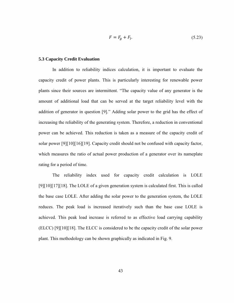
5.3 Capacity Credit Evaluation

In addition to reliability indices calculation, it is important to evaluate the

capacity credit of power plants. This is particularly interesting for renewable power

plants since their sources are intermittent. “The capacity value of any generator is the

amount of additional load that can be served at the target reliability level with the

addition of generator in question [9].” Adding solar power to the grid has the effect of

increasing the reliability of the generating system. Therefore, a reduction in conventional

power can be achieved. This reduction is taken as a measure of the capacity credit of

solar power [9][10][16][19]. Capacity credit should not be confused with capacity factor,

which measures the ratio of actual power production of a generator over its nameplate

rating for a period of time.

The reliability index used for capacity credit calculation is LOLE

[9][10][17][18]. The LOLE of a given generation system is calculated first. This is called

the base case LOLE. After adding the solar power to the generation system, the LOLE

reduces. The peak load is increased iteratively such than the base case LOLE is

achieved. This peak load increase is referred to as effective load carrying capability

(ELCC) [9][10][18]. The ELCC is considered to be the capacity credit of the solar power

plant. This methodology can be shown graphically as indicated in Fig. 9.

44

Figure 9 - Capacity credit evaluation method

The capacity value of solar power plant depends on a number of factors:

Solar radiation at the plant location

Solar plant components failure rate

Penetration level of solar power

Load model.

The solar radiation is the key factor in capacity value of solar plants.

Consequently, solar plants are constructed at locations with high levels of solar radiation

to increase its capacity value. The penetration level of solar power is also important

factor in capacity credit calculations. It is expected that higher penetration levels reduces

the capacity credit of solar plants. This is evaluated in case study of Chapter VI. The

load model is another important factor in capacity value of solar plants. Correlation

between load and solar radiation increases capacity value of solar plants.

45

CHAPTER VI

CASE STUDY

6.1 Introduction

The methodology developed in this thesis is evaluated in this chapter. In order to

compare the generation system reliability with and without solar power, a test system is

needed. The test system used in this thesis is IEEE Reliability Test System (IEEE-RTS).

This test system has generation and load data and it serves as our base system. The

generation system consists of conventional units. The solar power system is evaluated

within this system for five and twenty percent penetration levels. For this purpose, five

and twenty percent of the conventional power plants are replaced with the solar plants.

The reliability indices of the base case are compared with that of five and twenty percent

penetration of solar plants. In addition, capacity credits of solar power plants are

evaluated for five and twenty percent penetration levels.

6.2 IEEE Reliability Test System

The IEEE-RTS describes a load model, generation system and transmission

network which can be used to test or compare methods for reliability analysis of power

systems [20]. Since in this thesis, transmission network is not considered, we only use

the load model and the generation system.

46

6.2.1 Load Model

The annual peak load for the test system is 2850 MW. The weekly, daily, and

hourly peak loads as percentage of annual peak load are given in the Tables 14, 15, and

16. From these tables, we obtain the hourly load for the whole year. The year is

considered to be 52 weeks, which is 364 days. Therefore, the number of hours per year is

7836.

Table 14 - Weakly peak load in percent of annual peak

Week Peak Load Week Peak Load 1 86.2 27 75.5 2 90.0 28 81.6 3 87.8 29 80.1 4 83.4 30 88.0 5 88.0 31 72.2 6 84.1 32 77.6 7 83.2 33 80.0 8 80.6 34 72.9 9 74.0 35 72.6 10 73.7 36 70.5 11 71.5 37 78.0 12 72.7 38 69.5 13 70.4 39 72.4 14 75.0 40 72.4 15 72.1 41 74.3 16 80.0 42 74.4 17 75.4 43 80.0 18 83.7 44 88.1 19 87.0 45 88.5 20 88.0 46 90.9 21 85.6 47 94.0 22 81.1 48 89.0 23 90.0 49 94.2 24 88.7 50 97.0 25 89.6 51 100.0 26 86.1 52 95.2

47

Table 15 - Daily peak load in percent of weekly peak

Day Peak Load Monday 93 Tuesday 100 Wednesday 98 Thursday 96 Friday 94 Saturday 77 Sunday 75

Table 16 - Hourly peak load in percent of daily peak

Winter Weeks 1-8 & 44-52

Summer Weeks 18-30

Spring/Fall Weeks 9-17 &

31-43 Hour Wkdy Wknd Wkdy Wknd Wkdy Wknd 0-1 67 78 64 74 63 75 1-2 63 72 60 70 62 73 2-3 60 68 58 66 60 69 3-4 59 66 56 65 58 66 4-5 59 64 56 64 59 65 5-6 60 65 58 62 65 65 6-7 74 66 64 62 72 68 7-8 86 70 76 66 85 74 8-9 95 80 87 81 95 83 9-10 96 88 95 86 99 89 10-11 96 90 99 91 100 92 11-12 95 91 100 93 99 94 12-13 95 90 99 93 93 91 13-14 95 88 100 92 92 90 14-15 93 87 100 91 90 90 15-16 94 87 97 91 88 86 16-17 99 91 96 92 90 85 17-18 100 100 96 94 92 88 18-19 100 99 93 95 96 92 19-20 96 97 92 95 98 100 20-21 91 94 92 100 96 97 21-22 83 92 93 93 90 95 22-23 73 87 87 88 80 90 23-24 63 81 72 80 70 85

48

6.2.2 Generation System

Table 17 gives a list of the generating unit ratings and reliability data.

Table 17 - Base system generation units

Generating Unit Reliability Data Unit Size (MW) Number of Units Forced Outage Rate MTTF (hrs.) MTTR (hrs.)

12 5 0.02 2940 60 20 4 0.10 450 50 50 6 0.01 1980 20 76 4 0.02 1960 40 100 3 0.04 1200 50 155 4 0.04 960 40 197 3 0.05 950 50 350 1 0.08 1150 100 400 2 0.12 1100 150

MTTF = mean time to failure

MTTR = mean time to repair

Forced Outage Rate =

.

The generating units are of conventional type. This generation system consists of

9 distinct types of generating units and the total of 32 units. The total generation capacity

is 3405 MW.

This generation system serves as our base system. This generation system model

is constructed using unit addition algorithm. There are 3180 capacity outage levels in

this generation system model. The cumulative probability and frequency of each

capacity outage level is calculated. The results are tabulated as it is shown in Table 18. A

table with more capacity outage levels is available at Appendix.

49

Table 18 - Generation system model of the conventional subsystem

i Xi = Capacity Outage Levels Pi (Capout≥Xi) Fi (Capout≥Xi) 1 0 1 0 2 12 0.7636 58.18 … … … …

3180 3405 1.21×10-48 8.51×10-45

6.3 Generation System with Solar Units

In order to have a generation system with five and twenty percent solar

penetration, it is required to replace five and twenty percent of the conventional

generation capacity for the base system with solar power:

5% of the total capacity = 3405×0.05 = 170.25 MW

20% of the total capacity = 3405×0.20 = 681 MW.

We round the above capacity to 150 MW and 600 MW respectively for

convenience. These are for both PV and CSP units. The individual capacity for PV and

CSP plants for each penetration level is indicated in Table 19.

Table 19 - Solar power capacity used for different penetration levels

PV Capacity (MW) CSP Capacity (MW) 5% Penetration 50 100 20% Penetration 200 400

The generation system model is constructed for conventional, PV, and CSP

subsystems for five and twenty percent solar penetration levels.

50

6.3.1 Conventional Subsystem

For five percent penetration, the conventional subsystem capacity is 3255 MW.

In the base case generation system of IEEE-RTS, a 50 MW and a 100 MW unit is

removed and the generation system model is constructed again. The results are tabulated

as it is shown in Table 20.

Table 20 - Generation system model of the conventional subsystem for 5% solar penetration

i Xi = Capacity Outage Levels Pi (Capout≥Xi) Fi (Capout≥Xi) 1 0 1 0 2 12 0.7513 58.31 … … … …

3030 3255 3.20×10-45 1.94×10-41

For twenty percent penetration, the conventional subsystem capacity is 2805

MW. In the base case generation system of IEEE-RTS, two 50 MW, a 100 MW, and a

400 MW unit is removed and the generation system model is constructed again. The

results are tabulated as it is shown in Table 21.

Table 21 - Generation system model of the conventional subsystem for 20% solar penetration

i Xi = Capacity Outage Levels Pi (Capout≥Xi) Fi (Capout≥Xi) 1 0 1 0 2 12 0.7145 63.40 … … … …

2580 2805 2.52×10-42 1.49×10-38

51

6.3.2 PV Subsystem

The PV unit failure depends on the inverter failure or the transformer failure. The

reliability data for the inverter and the transformer is given in Table 22. This data is

estimated from values given in [4] and rounded off for simplicity. The accuracy of this

data is not critical in reliability evaluation of PV units; rather the PV plant configuration

is more important.

Table 22 - PV unit reliability data

Unit Size (MW)

Number of Units

Forced Outage Rate

MTTF (hrs.)

MTTR (hrs.)

Inverter 1 10 0.0909 2400 240 Transformer 10 1 0.0909 24000 2400

Unlike the conventional case, where the generating unit is a 2-state unit, the PV

unit is an 11-state unit. The PV unit capacity outage level is given in Table 23.

Table 23 - PV unit capacity outage levels

i Capacity Outage Level 1 0 2 1 3 2 4 3 5 4 6 5 7 6 8 7 9 8 10 9 11 10

52

For five and twenty percent solar penetration levels, different number of PV units

is used as given in Table 24.

Table 24 - Number of PV units for different penetration levels

PV Units Sola Penetration Level PV Size (MW) Unit Size (MW) Number of Units

5% 50 10 5 20% 200 10 20

For five percent penetration level, five PV units are used. The generation system

model is constructed for the PV subsystem and tabulated as Table 25 (complete table is

available in Appendix).

Table 25 - Generation system model of the PV subsystem for 5% solar penetration

i Xi = Capacity Outage Levels Pi (Capout≥Xi) Fi (Capout≥Xi) 1 0 1 0 2 1 0.9932 0.9856 … … … … 51 50 6.21×10-6 7.50×10-3

For twenty percent penetration level, twenty PV units are used. The generation

system model is constructed for the PV subsystem and tabulated as Table 26.

Table 26 - Generation system model of the PV subsystem for 20% solar penetration

i Xi = Capacity Outage Levels Pi (Capout≥Xi) Fi (Capout≥Xi) 1 0 1 0 2 1 0.9984 0.0304 … … … … 201 200 1.48×10-21 1.62×10-18

53

6.3.3 CSP Subsystem

The CSP unit is treated in the same manner as conventional units. Therefore, we

use the same reliability indices as the conventional unit. This is given in Table 27.

Table 27 - CSP unit reliability data

CSP Unit Reliability Data Solar

Penetration Level

CSP size (MW) Unit Size

(MW) Number of

Units

Forced Outage

Rate

MTTF (hrs.)

MTTR (hrs.)

5% 100 100 1 0.04 1200 50 20% 400 400 1 0.12 1100 150

For five percent penetration level, a 100 MW unit is used. The generation system

model is constructed for the CSP subsystem and tabulated as Table 28.

Table 28 - Generation system model of the CSP subsystem for 5% solar penetration

i Xi = Capacity Outage Levels Pi (Capout≥Xi) Fi (Capout≥Xi) 1 0 1 0 2 100 0.04 6.99

For twenty percent penetration level, a 400 MW unit is used. The generation

system model is constructed for the CSP subsystem and tabulated as Table 29.

Table 29 - Generation system model of the CSP subsystem for 20% solar penetration

i Xi = Capacity Outage Levels Pi (Capout≥Xi) Fi (Capout≥Xi) 1 0 1 0 2 400 0.12 6.99

54

6.4 Solar Radiation Effect

Once generation system model is constructed for PV and CSP subsystems, the

effect of solar radiation needs to be considered. For this purpose, hourly radiation data at

plant location is measured. In this thesis, the radiation data is obtained from National

Renewable Energy Laboratory (NREL) solar radiation data. These measurements are

conducted by Solar Radiation Research Laboratory (SRRL). The measurement type used

is called Base Measurement System (BMS) that provides solar radiation data from

instruments at the NREL South Table Mountain site in Golden, Colorado. The latitude,

longitude, and elevation of the site are 39.74 °N, 105.18 °W, and 1829 m, respectively.

The measurements used in this case study are hourly solar radiation for year 2012.

There are different types of solar radiation data. As discussed in Chapter IV, for

PV plants global solar radiation is needed. This radiation measurement is available at

different angles. Since PV panels are tilted at a fixed angle proportional to the site

latitude, hourly global solar radiation on a 40-degree south facing surface is used to

measure the PV plant output power. For CSP plants, hourly direct normal solar radiation

is used to measure the CSP plant output power.

Once these measurements are obtained, the generation system model for PV and

CSP subsystems are modified to incorporate the effect of radiation. This was explained

is Chapter IV.

55

6.5 Reliability Indices Calculation

Once the load model and the generation system model for each subsystem are

constructed, the reliability indices can be obtained by the methods developed in Chapter

V. This is done for the base case system, five percent solar penetration, and twenty

percent solar penetration.

6.5.1 Results

The reliability indices are calculated and the results are summarized in Table 30.

Table 30 - Reliability indices calculation

LOLE (h/year) EUE (MWh) Freq (/year) Base Case 9.39 1,176 1.83

5% Penetration 19.06 2,716 3.84

20% Penetration 90.40 20,884 85.47

6.5.2 Discussion

Based on the results obtained above, the reliability of generation system is

reduced after replacing solar generators with conventional generators. This is as

expected since solar generators are not dispatchable and their power generation depends

on solar radiation that is intermittent in nature. As the penetration level of solar power

increases, the reliability is reduced further. This reduction is more intense for higher

penetration levels.

56

6.6 Capacity Credit Evaluation

After reliability indices are calculated, capacity credit of solar power plants can

be evaluated using the LOLE index.

6.6.1 Results

In order to evaluate the capacity credit of solar plant for five percent solar

penetration, the LOLE of the conventional subsystem for five percent solar penetration is

calculated first. Then, the solar units are added for five percent penetration level to this

conventional subsystem and the LOLE is calculated. The results are given in Table 31.

Table 31 - LOLE before and after adding solar units for 5% penetration

Conventional Capacity (MW)

Conventional LOLE (h/yr)

LOLE after adding solar units (h/yr)

3255 26.12 19.06

For capacity credit evaluation, the peak load is iteratively increased until the

conventional LOLE is achieved. The results are given in Table 32:

Table 32 - Peak load increase for capacity credit evaluation

Peak Load Increase (MW) LOLE (h/yr) 53 26.16 52 26.02

Based on above data, capacity credit of 150 MW solar power plant is between 53

to 52 MW. Since the LOLE corresponding to 53 MW peak load increase is closer to

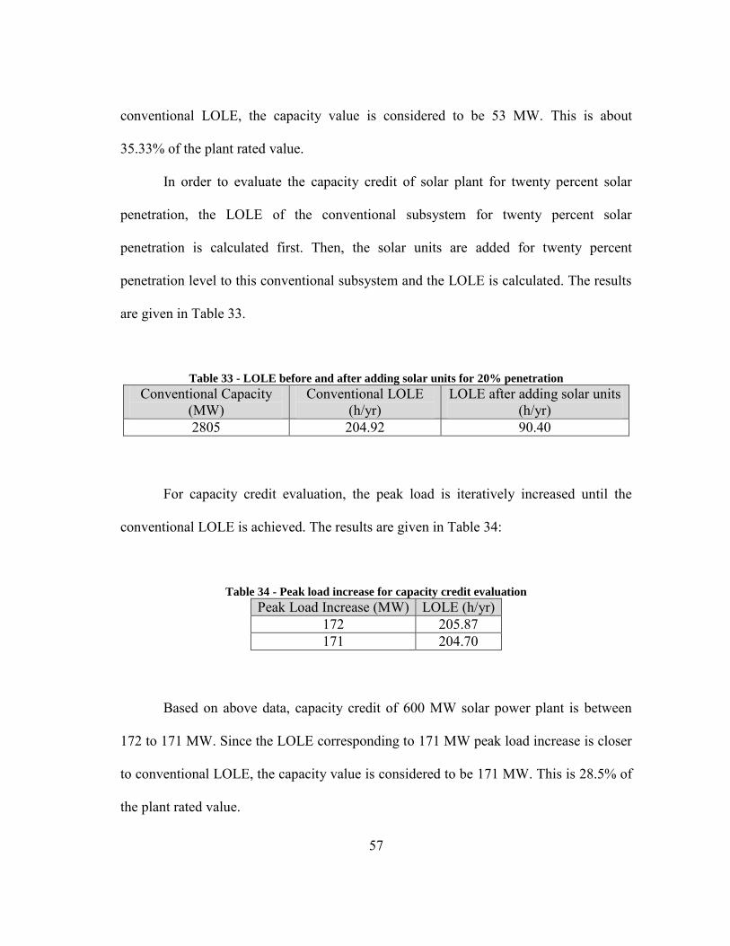
57

conventional LOLE, the capacity value is considered to be 53 MW. This is about

35.33% of the plant rated value.

In order to evaluate the capacity credit of solar plant for twenty percent solar

penetration, the LOLE of the conventional subsystem for twenty percent solar

penetration is calculated first. Then, the solar units are added for twenty percent

penetration level to this conventional subsystem and the LOLE is calculated. The results

are given in Table 33.

Table 33 - LOLE before and after adding solar units for 20% penetration

Conventional Capacity (MW)

Conventional LOLE (h/yr)

LOLE after adding solar units (h/yr)

2805 204.92 90.40

For capacity credit evaluation, the peak load is iteratively increased until the

conventional LOLE is achieved. The results are given in Table 34:

Table 34 - Peak load increase for capacity credit evaluation

Peak Load Increase (MW) LOLE (h/yr) 172 205.87 171 204.70

Based on above data, capacity credit of 600 MW solar power plant is between

172 to 171 MW. Since the LOLE corresponding to 171 MW peak load increase is closer

to conventional LOLE, the capacity value is considered to be 171 MW. This is 28.5% of

the plant rated value.

58

6.6.2 Discussion

Based on above calculations, capacity value of solar power plants reduces as

penetration levels of solar plants increase. In this experiment, other factors affecting the

capacity credit such as radiation, components failure, and load remained to be constant.

59

CHAPTER VII

CONCLUSION

This thesis developed a methodology for quantitative reliability study of

generation systems with solar power and to evaluate capacity credit of solar power

plants. This methodology assists power system planners in designing generation systems

with renewable power, in particular solar power, which meets the required reliability

standards. Peaking units required to backup renewable power plants can be determined

using this method. It also helps to compare the cost of conventional power plants with

the effective value of renewable power plants.

The primary step in reliability evaluation of solar power plant is modeling the

solar generation units. This was done separately for PV and CSP units. PV units were

modeled as a multistate unit depending on the number of inverters. CSP units were

modeled same as conventional units. After unit models were developed, the generation

system model was constructed for each subsystem. These generation subsystem models

were used along with load model to calculate the reliability indices of the generation

system with solar power for different penetration levels. In addition, capacity credit of

solar power plants was evaluated for different penetration levels.

The reliability of electric power generation system deteriorates if conventional

generators are replaced with solar generators. This deterioration is more severe for larger

penetrations of solar units. On the other hand, addition of solar generators improves

reliability of the generation system, but this improvement is less than their plant ratings.

60

From this improvement, the capacity credit of solar power plants was evaluated. This

capacity credit was about 35.33% of plant rating for five percent penetration level and

28.5% of plant rating for twenty percent penetration level. Knowledge of this capacity

value is important for electric power system generation planning. The conventional

practice is to have a peaking unit as a backup for every MW of solar or any renewable

unit. This is applicable if capacity value of the renewable plant is zero. However, using

capacity value of solar plants, the need for peaking unit as a backup is less than the solar

plant rating and can be quantitatively calculated.

61

REFERENCES

1. Xie, L., Carvalho, P., Ferreira, L., Liu, J., Krogh, B., Popli, N., Ilic, M., “Wind Integration in Power Systems: Operational Challenges and Possible Solutions,” Proceedings of the IEEE, Vol. 99, No. 1, pp. 214-232, Jan. 2011.

2. De Meo, E. A., Grant, W., Milligan, M. R., Schuerger, M. J., “Wind Plant Integration,” IEEE Power and Energy Magazine, Vol. 3, No. 6, pp. 38-46, Nov.-Dec. 2005.

3. Deshmukh, R. G., “A Probabilistic Study of Wind Electric Conversion Systems from the Point of View of Reliability and Capacity Credit.” Dissertation submitted to the graduate college of the Oklahoma State University, May 1979.

4. Stember, L. H., Huss, W. R., Bridgman, M. S., “A Methodology for Photovoltaic System Reliability and Economic Analysis,” IEEE Transactions on Reliability, Vol. R-31, pp. 296-303, Aug. 1982.

5. Singh, C., Gonzalez, A., “Reliability Modeling of Generation Systems Including Unconventional Energy Sources,” IEEE Transactions on Power Apparatus and Systems, Vol. PAS-104, No. 5, pp. 1049-1056, May 1985.

6. Singh, C., Kim, Y., “An Efficient Technique for Reliability Analysis of Power Systems Including Time Dependent Sources,” IEEE Transactions on Power Systems, Vol. 3, No. 3, pp. 1090-1096, Aug. 1988.

7. Fockens, S., Wijk, A., Turkenburg, W., Singh, C., “A Concise Method for Calculating Expected Unserved Energy in Generating System Reliability Analysis,” IEEE Transactions on Power Systems, Vol. 6, No. 3, pp. 1085-1091, Aug. 1991.

8. Zhang, P., Wang, Y., Xiao, W., Li, W., “Reliability Evaluation of Grid-Connected Photovoltaic Power Systems,” IEEE Transactions on Sustainable Energy, Vol. 3, No. 3, pp. 379-389, July 2012.

9. Ensslin, C., Milligan, M., Holttinen, H., O’Malley, M., Keane, A., “Current Methods to Calculate Capacity Credit of Wind Power, IEA Collaboration,” Power and Energy Society General Meeting, pp. 1-3, July 2008.

10. Keane, A., Milligan, M., Dent, C. J., Hasche, B., D’Annunzio, C., Dragoon, K., Holtinnen, H., Samaan, N., Soder, L., O’Malley, M., “Capacity Value of Wind Power,” IEEE Transactions on Power Systems, Vol. 26, No. 2, pp. 564-572, May 2011.

62

11. Singh, C., Billinton, R. “System Reliability Modelling and Evaluation,” 1st ed. London, U.K.: Hutchinson Educational, Jun. 1977.

12. National Renewable Energy Laboratory, “Concentrating Solar Power,” Aug. 2010. <http://www.nrel.gov/csp/pdfs/48658.pdf>.

13. Denholm, P., Mehos, M., “Enabling Greater Penetration of Solar Power via the Use of CSP with Thermal Energy Storage,” Technical Report No. TP-6A20-52978. National Renewable Energy Laboratory, Golden, CO, USA.

14. Denholm, P., Wan, Y. H., Hummon, M., Mehos, M., “An Analysis of Concentrating Solar Power with Thermal Energy Storage in a California 33% Renewable Scenario.” Technical Report No. TP-6A20-58186. National Renewable Energy Laboratory, Golden, CO, USA.

15. Energy Department, “Concentrating Solar Power,” <http://energy.gov/energybasics/articles/concentrating-solar-power >.

16. Wang, L., Singh, C., “An Alternative Method for Estimating Wind-Power Capacity Credit based on Reliability Evaluation Using Intelligent Search.” Proceedings of the 10th International Conference on Probabilistic Methods Applied to Power Systems, PMAPS 08, pp. 1-6, May 2008.

17. Castro, R. M. G., Ferreira, L. A. F., “A Comparison Between Chronological and Probabilistic Methods to Estimate Wind Power Capacity Credit,” IEEE Transaction on Power System, Vol. 16, No. 4, pp. 904-909, Nov. 2001.

18. Perez, R., Taylor, M., Hoff, T., Ross, J. P., “Reaching Consensus in the Definition of Photovoltaics Capacity Credit in the USA: A Practical Application of Satellite-Drived Solar Resource Data,” IEEE Journal of Selected Topics in Applied Earth Observations and Remote Sensing, Vol. 1, No. 1, pp. 28-33, Oct. 2008.

19. Wang, L., Singh, C., “A New Method for Capacity Credit Estimation of Wind Power,” Fifteenth National Power Systems Conference (NPSC), IIT, Bombay, India, Dec. 2008.

20. Subcommittee, P. M., “IEEE Reliability Test System,” IEEE Transaction on Power Apparatus and Systems, Vol. PAS-98, No. 6, pp. 2047-2054, Nov. 1979.

63

APPENDIX

Generation system model of conventional subsystem (first 100 capacity outage

levels) is given in Table A-1. Generation system models of PV subsystem for 5% solar

penetration and 20% solar penetration are given in Tables A-2 and A-3.

Table A-1 Generation system model of conventional subsystem

i Capacity Outage P F(/yr)

1 0 1 0

2 12 0.763602474 58.18169865

3 20 0.739482306 60.53445631

4 24 0.634416739 65.99626029

5 32 0.633432631 65.94598186

6 36 0.622712557 64.90269193

7 40 0.622692623 64.90644287

8 44 0.605181696 62.41728874

9 48 0.604744315 62.35788851

10 50 0.604744112 62.31006777

11 52 0.590416989 59.51493109

12 56 0.58863031 58.99288943

13 60 0.58862145 58.9919778

14 62 0.587324345 58.55578456

15 64 0.585862516 58.05339953

16 68 0.585789619 58.03200657

17 70 0.585789596 58.02134665

18 72 0.579421986 55.5428983

19 74 0.579289594 55.47844619

20 76 0.579229951 55.44908387

21 80 0.559930695 55.89738987

22 82 0.559894664 55.87827624

23 84 0.559244963 55.52839037

24 86 0.559239563 55.5255628

25 88 0.559238355 55.52525711

26 90 0.557269356 55.27791644

27 92 0.556208088 54.65881416

28 94 0.556204407 54.65630756

64

Table A-1 Continued

i Capacity Outage P F(/yr)

29 96 0.556177899 54.64101193

30 98 0.547601003 53.17540163

31 100 0.547600991 53.17249797

32 102 0.517609169 54.8149456

33 104 0.517500885 54.73553068

34 106 0.517500735 54.7354068

35 108 0.517500198 54.73511465

36 110 0.516625089 54.45492318

37 112 0.516546477 54.39380245

38 114 0.513492914 54.11013312

39 116 0.513488496 54.10688729

40 118 0.512059029 53.58512186

41 120 0.512059028 53.5844751

42 122 0.498729329 51.73061972

43 124 0.498721305 51.72317346

44 126 0.498596769 51.68918679

45 128 0.497427117 51.20029226

46 130 0.497281266 51.12517256

47 132 0.497279082 51.12305069

48 134 0.495921943 50.73244786

49 136 0.495921616 50.7321321

50 138 0.495813207 50.6729212

51 140 0.495693874 50.60527958

52 142 0.493472257 49.8652309

53 144 0.493472034 49.86498056

54 146 0.493416691 49.84605291

55 148 0.492896879 49.52788076

56 150 0.492886045 49.51415516

57 152 0.491085414 48.83008864

58 154 0.490268474 48.60298918

59 155 0.490268465 48.60297766

60 156 0.450868878 49.33652124

61 158 0.450864815 49.3339766

62 160 0.450811778 49.29359477

63 162 0.450647214 49.20681307

64 164 0.45046389 49.11010183

65 166 0.45039439 49.08460305

66 167 0.450307756 49.01475678

67 168 0.446287728 48.49232667

65

Table A-1 Continued

i Capacity Outage P F(/yr)

68 170 0.446287425 48.49070572

69 172 0.445487144 48.03155175

70 174 0.445207828 47.91682222

72 176 0.427689424 44.83809449

73 178 0.425245021 44.42847511

74 179 0.425236181 44.42002232

75 180 0.425072164 44.37432852

76 182 0.425067592 44.37102886

77 184 0.424986115 44.31216482

78 186 0.424958642 44.29712943

79 187 0.424952074 44.29064367

80 188 0.423165395 43.71029251

81 190 0.422916206 43.63152969

82 191 0.422782826 43.52912365

83 192 0.422779504 43.528993

84 194 0.422735279 43.50286247

85 195 0.422731956 43.50028148

86 196 0.419813468 42.42146644

87 197 0.418727137 42.02867894

88 198 0.381401212 44.35043594

89 199 0.381400555 44.34931788

90 200 0.381327658 44.32283382

91 202 0.380040994 44.13578911

92 203 0.379991612 44.10038871

93 204 0.379991578 44.09241089

94 205 0.379987094 44.08909699

95 206 0.37759924 43.08000414

96 207 0.377598995 43.07974221

97 208 0.377301215 42.92499035

98 209 0.377190465 42.86843487

99 210 0.375920982 42.46820007

100 211 0.373372137 42.52998463

Table A-2 Generation system model of PV subsystem for 5% solar penetration

i Capacity Outage P F(/yr)

1 0 1 0

2 1 0.993195889 0.985616365

66

Table A-2 Continued

i Capacity Outage P F(/yr)

3 2 0.966103362 4.477472954

4 3 0.900963951 10.24042233

5 4 0.79735258 15.49899255

6 5 0.675882592 17.39271743

7 6 0.56424722 15.39446755

8 7 0.480568047 11.16953877

9 8 0.427987459 6.819318776

10 9 0.399731489 3.569965819

11 10 0.386547279 3.761736379

12 11 0.374108163 10.12203007

13 12 0.344648796 20.33133567

14 13 0.290584017 27.60970596

15 14 0.222818697 27.50539363

16 15 0.160300093 21.3209216

17 16 0.115326349 13.36515875

18 17 0.089101543 6.957522015

19 18 0.076366235 3.066373509

20 19 0.071113505 1.160990736

21 20 0.069245997 2.581290193

22 21 0.065097902 7.074146904

23 22 0.054281082 10.57771531

24 23 0.038802345 10.28446068

25 24 0.024389424 7.249345462

26 25 0.014666936 3.780856545

27 26 0.009612459 1.635342526

28 27 0.007506664 0.565394894

29 28 0.00678472 0.164891065

30 29 0.006577168 0.101058495

31 30 0.006526434 0.842467254

32 31 0.005593307 1.655095441

33 32 0.003748998 1.592059173

34 33 0.001998969 0.974974239

35 34 0.000949252 0.425123271

36 35 0.000503167 0.123559024

37 36 0.000360425 0.031726856

38 37 0.00032474 0.006512952

39 38 0.000317603 0.001084955

40 39 0.000316444 0.018420809

41 40 0.000316289 0.131948276

67

Table A-2 Continued

i Capacity Outage P F(/yr)

42 41 0.000196686 0.127638936

43 42 7.71683E-05 0.056557922

44 43 2.33857E-05 0.015426124

45 44 9.04373E-06 0.002736297

46 45 6.53388E-06 0.000333486

47 46 6.2327E-06 2.82525E-05

48 47 6.2076E-06 1.64206E-06

49 48 6.20616E-06 6.26443E-08

50 49 6.20611E-06 0.002033123

51 50 6.20611E-06 0.007544914

Table A-3 Generation system model of PV subsystem for 20% solar penetration

i Capacity Outage P F(/yr)

1 0 1 0

2 1 0.998448062 0.030433052

3 2 0.997611989 0.046494569

4 3 0.996785211 0.059763479

5 4 0.996035882 0.07062748

6 5 0.995355802 0.080958464

7 6 0.9947263 0.095761263

8 7 0.994111927 0.12660491

9 8 0.993439105 0.196240136

10 9 0.992567785 0.342078959

11 10 0.991262775 0.623093576

12 11 2.339071402 -11.6590125

13 12 1.335543111 8.776376538

14 13 1.137723788 6.873206412

15 14 1.014834232 4.993592251

16 15 0.970538375 5.090803982

17 16 0.952221413 5.940407374

18 17 0.937672454 6.799774538

19 18 0.922429083 7.487406932

20 19 0.906232069 8.057104922

21 20 0.889193527 5.034664631

22 21 0.961990233 13.17122156

23 22 0.851407085 10.76474778

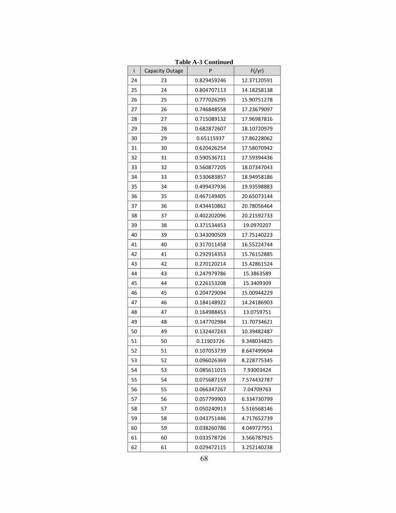
68

Table A-3 Continued

i Capacity Outage P F(/yr)

24 23 0.829459246 12.37120591

25 24 0.804707113 14.18258138

26 25 0.777026295 15.90751278

27 26 0.746848558 17.23679097

28 27 0.715089132 17.96987816

29 28 0.682872607 18.10720979

30 29 0.65115937 17.86228062

31 30 0.620426254 17.58070942

32 31 0.590536711 17.59394436

33 32 0.560877205 18.07347043

34 33 0.530683857 18.94958186

35 34 0.499437936 19.93598883

36 35 0.467149405 20.65073144

37 36 0.434410862 20.78056464

38 37 0.402202096 20.21592733

39 38 0.371534453 19.0970207

40 39 0.343090509 17.75140223

41 40 0.317011458 16.55224744

42 41 0.292914353 15.76152885

43 42 0.270120214 15.42861524

44 43 0.247979786 15.3863589

45 44 0.226153208 15.3409309

46 45 0.204729094 15.00944229

47 46 0.184148922 14.24186903

48 47 0.164988453 13.0759751

49 48 0.147702984 11.70734621

50 49 0.132447243 10.39482487

51 50 0.11903726 9.348034825

52 51 0.107053739 8.647499694

53 52 0.096026369 8.228775345

54 53 0.085611015 7.93003424

55 54 0.075687159 7.574432787

56 55 0.066347267 7.04709763

57 56 0.057799903 6.334730799

58 57 0.050240913 5.516568146

59 58 0.043751446 4.717652739

60 59 0.038260786 4.049727951

61 60 0.033578726 3.566787925

62 61 0.029472115 3.252140238

69

Table A-3 Continued

i Capacity Outage P F(/yr)

63 62 0.025745835 3.037492708

64 63 0.022293575 2.8403219

65 64 0.019103244 2.600172033

66 65 0.016223953 2.298701012

67 66 0.013716176 1.958272245

68 67 0.011609062 1.623929423

69 68 0.009880884 1.339512363

70 69 0.008465753 1.129037053

71 70 0.007278183 0.990160666

72 71 0.006241357 0.900075093

73 72 0.005306386 0.828696345

74 73 0.004456543 0.751926561

75 74 0.003698244 0.659398422

76 75 0.003045671 0.554814661

77 76 0.00250688 0.450537551

78 77 0.002076597 0.360016105

79 78 0.001736917 0.291649879

80 79 0.001463601 0.246249246

81 80 0.001233895 0.218241936

82 81 0.001032175 0.199164638

83 82 0.000851555 0.181408563

84 83 0.000691849 0.160654768

85 84 0.000555693 0.136411182

86 85 0.000444914 0.110962613

87 86 0.000358518 0.087562877

88 87 0.000292614 0.068778004

89 88 0.000241736 0.055590537

90 89 0.000200597 0.047382554

91 90 0.000165413 0.042514561

92 91 0.000134329 0.039093197

93 92 0.000107026 0.035617642

94 93 8.39107E-05 0.031341551

95 94 6.53373E-05 0.026298958

96 95 5.11655E-05 0.021046766

97 96 4.07092E-05 0.016282324

98 97 3.29691E-05 0.012526121

99 98 2.69583E-05 0.009972695

100 99 2.19536E-05 0.008493624

101 100 1.75822E-05 0.00773229

70

Table A-3 Continued

i Capacity Outage P F(/yr)

102 101 1.3757E-05 0.007249309

103 102 1.05331E-05 0.006681898

104 103 7.97055E-06 0.005858076

105 104 6.05569E-06 0.004812339

106 105 4.6893E-06 0.003707577

107 106 3.72143E-06 0.002726661

108 107 3.00179E-06 0.001995362

109 108 2.41891E-06 0.001551553

110 109 1.91421E-06 0.001347495

111 110 1.47261E-06 0.001277646

112 111 1.10113E-06 0.001227006

113 112 8.08656E-07 0.001119722

114 113 5.94588E-07 0.000940864

115 114 4.47032E-07 0.000722514

116 115 3.4737E-07 0.00051185

117 116 2.76769E-07 0.000345793

118 117 2.21213E-07 0.000240916

119 118 1.73337E-07 0.000192973

120 119 1.31239E-07 0.0001817

121 120 9.5786E-08 0.000181002

122 121 6.81194E-08 0.000171252

123 122 4.82998E-08 0.000146306

124 123 3.51348E-08 0.000111516

125 124 2.67016E-08 7.63065E-05

126 125 2.10516E-08 4.7982E-05

127 126 1.67408E-08 2.97923E-05

128 127 1.30203E-08 2.1408E-05

129 128 9.70896E-09 1.9782E-05

130 129 6.90799E-09 2.05775E-05

131 130 4.74157E-09 2.02601E-05

132 131 3.22579E-09 1.75457E-05

133 132 2.25926E-09 1.31896E-05

134 133 1.67652E-09 8.68069E-06

135 134 1.31136E-09 5.09422E-06

136 135 1.04202E-09 2.81032E-06

137 136 8.06814E-10 1.75578E-06

138 137 5.92728E-10 1.57892E-06

139 138 4.10129E-10 1.756E-06

140 139 2.70357E-10 1.82412E-06

71

Table A-3 Continued

i Capacity Outage P F(/yr)

141 140 1.75242E-10 1.60089E-06

142 141 1.17361E-10 1.17682E-06

143 142 8.48526E-11 7.35659E-07

144 143 6.61224E-11 4.00099E-07

145 144 5.2828E-11 1.95477E-07

146 145 4.08756E-11 1.01427E-07

147 146 2.95767E-11 8.72842E-08

148 147 1.98174E-11 1.09395E-07

149 148 1.24516E-11 1.23305E-07

150 149 7.61396E-12 1.09803E-07

151 150 4.82943E-12 7.78747E-08

152 151 3.39248E-12 4.5234E-08

153 152 2.65134E-12 2.21976E-08

154 153 2.14976E-12 9.59505E-09

155 154 1.67056E-12 3.91091E-09

156 155 1.18892E-12 2.97472E-09

157 156 7.65793E-13 4.73725E-09

158 157 4.53125E-13 6.13522E-09

159 158 2.5763E-13 5.55583E-09

160 159 1.52784E-13 3.70872E-09

161 160 1.03914E-13 1.92222E-09

162 161 8.23094E-14 8.09177E-10

163 162 6.87016E-14 2.94563E-10

164 163 5.39948E-14 1.04995E-10

165 164 3.7672E-14 4.34285E-11

166 165 2.30314E-14 1.24482E-10

167 166 1.25784E-14 2.17018E-10

168 167 6.49611E-15 2.00891E-10

169 168 3.54513E-15 1.1956E-10

170 169 2.32882E-15 5.06875E-11

171 170 1.89656E-15 1.64125E-11

172 171 1.66588E-15 4.59408E-12

173 172 1.33935E-15 1.55986E-12

174 173 9.10103E-16 8.16294E-13

175 174 5.15845E-16 4.74766E-13

176 175 2.50651E-16 5.10497E-12

177 176 1.12881E-16 4.96499E-12

178 177 5.54747E-17 2.22355E-12

179 178 3.58217E-17 5.9362E-13

72

Table A-3 Continued

i Capacity Outage P F(/yr)

180 179 3.0166E-17 1.05571E-13

181 180 2.87835E-17 2.14772E-14

182 181 2.43105E-17 1.67369E-14

183 182 1.5894E-17 1.44127E-14

184 183 7.94067E-18 8.47099E-15

185 184 3.17271E-18 3.56753E-15

186 185 1.14672E-18 1.06433E-13

187 186 4.98432E-19 2.82227E-16

188 187 3.36364E-19 5.6367E-17

189 188 3.03951E-19 9.1554E-18

190 189 2.98684E-19 3.36658E-17

191 190 2.97981E-19 2.252E-16

192 191 1.83614E-19 2.1172E-16

193 192 6.93332E-20 9.27428E-17

194 193 1.79095E-20 2.45046E-17

195 194 4.19661E-21 4.26465E-18

196 195 1.79686E-21 5.1039E-19

197 196 1.50889E-21 4.24885E-20

198 197 1.48489E-21 2.4279E-21

199 198 1.48352E-21 9.11083E-23

200 199 1.48347E-21 4.85986E-19

201 200 1.48347E-21 2.64046E-18