Embed Size (px)
Citation preview
GENFGeneration ofFinite Elementsand Beam Structures
Version 10.20
� SOFiSTiK AG, Oberschleissheim, 2001
GENF Definition of Finite Ele�
ments
This manual is protected by copyright laws. No part of it may be translated, copied orreproduced, in any form or by any means, without written permission from SOFiSTiKAG. SOFiSTiK reserves the right to modify or to release new editions of this manual.
The manual and the program have been thoroughly checked for errors. However,SOFiSTiK does not claim that either one is completely error free. Errors and omissionsare corrected as soon as they are detected.The user of the program is solely responsible for the applications. We stronglyencourage the user to test the correctness of all calculations at least by randomsampling.
GENFDefinition of Finite Elements
i
1 Task Description 1−1. . . . . . . . . . . . . . . . . . . . . . . . . . . . . . . . . . . . . . . .
2 Theoretical Principles 2−1. . . . . . . . . . . . . . . . . . . . . . . . . . . . . . . . . . .
2.1. Systems of Coordinates 2−1. . . . . . . . . . . . . . . . . . . . . . . . . . . . . . . . . . 2.2. Overview of the Element Types 2−2. . . . . . . . . . . . . . . . . . . . . . . . . . . 2.3. Mesh Partitioning 2−5. . . . . . . . . . . . . . . . . . . . . . . . . . . . . . . . . . . . . . . 2.4. Plane Elements 2−7. . . . . . . . . . . . . . . . . . . . . . . . . . . . . . . . . . . . . . . . . 2.5. Solid Elements 2−8. . . . . . . . . . . . . . . . . . . . . . . . . . . . . . . . . . . . . . . . . 2.6. Boundary Conditions 2−8. . . . . . . . . . . . . . . . . . . . . . . . . . . . . . . . . . . . 2.7. Girders 2−12. . . . . . . . . . . . . . . . . . . . . . . . . . . . . . . . . . . . . . . . . . . . . . . . 2.8. Literature 2−13. . . . . . . . . . . . . . . . . . . . . . . . . . . . . . . . . . . . . . . . . . . . . . 2.9. Limitations 2−13. . . . . . . . . . . . . . . . . . . . . . . . . . . . . . . . . . . . . . . . . . . .
3 Input Description 3−1. . . . . . . . . . . . . . . . . . . . . . . . . . . . . . . . . . . . . . .
3.1. Nodes 3−1. . . . . . . . . . . . . . . . . . . . . . . . . . . . . . . . . . . . . . . . . . . . . . . . . 3.2. Elements 3−1. . . . . . . . . . . . . . . . . . . . . . . . . . . . . . . . . . . . . . . . . . . . . . 3.3. Results 3−2. . . . . . . . . . . . . . . . . . . . . . . . . . . . . . . . . . . . . . . . . . . . . . . . 3.4. Restart 3−2. . . . . . . . . . . . . . . . . . . . . . . . . . . . . . . . . . . . . . . . . . . . . . . . 3.5. Input Records 3−3. . . . . . . . . . . . . . . . . . . . . . . . . . . . . . . . . . . . . . . . . . 3.6. ECHO − Control of the Output 3−7. . . . . . . . . . . . . . . . . . . . . . . . . . . 3.7. SYST − Global System Parameters 3−8. . . . . . . . . . . . . . . . . . . . . . . . 3.8. NODE − Nodal Coordinates and Constraints 3−12. . . . . . . . . . . . . . . 3.9. INTE − Intermediate Nodes 3−18. . . . . . . . . . . . . . . . . . . . . . . . . . . . . 3.10. KINE − Kinematic Dependencies 3−22. . . . . . . . . . . . . . . . . . . . . . . . . 3.11. MESH − Generation of Nodes and Quadrilateral Elements 3−23. . . 3.12. IMES − Generation of Irregular Nodes, Quadrilateral Elements . 3−273.13. CUBE − Nodes and Cubic Elements 3−29. . . . . . . . . . . . . . . . . . . . . . 3.14. TRAN − Transformation of Nodes 3−31. . . . . . . . . . . . . . . . . . . . . . . . 3.15. MIRR − Mirroring of Nodes 3−33. . . . . . . . . . . . . . . . . . . . . . . . . . . . . 3.16. ALIN − Node upon a Line (Projection to the Line) 3−36. . . . . . . . . . 3.17. SECT − Node at Intersection of two Straight Lines 3−39. . . . . . . . . . 3.18. Materials 3−41. . . . . . . . . . . . . . . . . . . . . . . . . . . . . . . . . . . . . . . . . . . . . . 3.19. NORM − Default Design Code 3−43. . . . . . . . . . . . . . . . . . . . . . . . . . . 3.20. MAT − General Material Properties 3−44. . . . . . . . . . . . . . . . . . . . . . . 3.21. MATE − Material Properties 3−45. . . . . . . . . . . . . . . . . . . . . . . . . . . . . 3.22. MLAY − Layered Material 3−48. . . . . . . . . . . . . . . . . . . . . . . . . . . . . . . 3.23. BMAT − Elastic Support / Interface 3−49. . . . . . . . . . . . . . . . . . . . . . . 3.24. NMAT − Nonlinear Material 3−52. . . . . . . . . . . . . . . . . . . . . . . . . . . . . 3.25. MEXT − Extra Materialconstants 3−63. . . . . . . . . . . . . . . . . . . . . . . . .

GENF Definition of Finite Elements
ii
3.26. CONC − Properties of Concrete 3−64. . . . . . . . . . . . . . . . . . . . . . . . . . 3.27. STEE − Properties of Metals 3−71. . . . . . . . . . . . . . . . . . . . . . . . . . . . . 3.28. TIMB − Properties of Timber 3−80. . . . . . . . . . . . . . . . . . . . . . . . . . . . 3.29. MASO − Masonry / Brickwork 3−82. . . . . . . . . . . . . . . . . . . . . . . . . . . . 3.30. SSLA − Stress−Strain Curves 3−84. . . . . . . . . . . . . . . . . . . . . . . . . . . . 3.31. SVAL − Cross−section values 3−86. . . . . . . . . . . . . . . . . . . . . . . . . . . . 3.32. SREC − Rectangle, T−beam, Plate 3−91. . . . . . . . . . . . . . . . . . . . . . . 3.33. SCIR − Circular and Annular Sections 3−94. . . . . . . . . . . . . . . . . . . . . 3.34. BORE − Bore Profile of a Sondation 3−95. . . . . . . . . . . . . . . . . . . . . . 3.35. BLAY − Layer of the Soil Strata 3−96. . . . . . . . . . . . . . . . . . . . . . . . . . 3.36. BBAX − Input of Axial Subgrade Parameters 3−97. . . . . . . . . . . . . . . 3.37. BBLA − Input of Lateral Subgrade Parameters 3−98. . . . . . . . . . . . . 3.38. HING − Hinged Connection Combinations for Beams 3−100. . . . . . . 3.39. GRP − Group Control 3−101. . . . . . . . . . . . . . . . . . . . . . . . . . . . . . . . . . 3.40. TRUS − Truss−bar Elements 3−105. . . . . . . . . . . . . . . . . . . . . . . . . . . . 3.41. CABL − Cable Elements 3−106. . . . . . . . . . . . . . . . . . . . . . . . . . . . . . . . 3.42. BEAM − Beam Elements 3−108. . . . . . . . . . . . . . . . . . . . . . . . . . . . . . . . 3.43. ADEF − Beginning of Beam Segment Definition 3−116. . . . . . . . . . . . 3.44. BDIV − Input of Beam Segments 3−117. . . . . . . . . . . . . . . . . . . . . . . . . 3.45. BSEC − Beam Sections 3−119. . . . . . . . . . . . . . . . . . . . . . . . . . . . . . . . . . 3.46. SUPP − Definition of Support Sections 3−120. . . . . . . . . . . . . . . . . . . . 3.47. QUAD − Plane Elements (Disks / Plates / Shells) 3−122. . . . . . . . . . . . 3.48. BRIC − Three−dimensional Solid Elements 3−126. . . . . . . . . . . . . . . . 3.49. SPRI − Spring Elements 3−127. . . . . . . . . . . . . . . . . . . . . . . . . . . . . . . . . 3.50. BOUN − Distributed Elastic Support 3−134. . . . . . . . . . . . . . . . . . . . . . 3.51. FLEX − General Elastic Element 3−139. . . . . . . . . . . . . . . . . . . . . . . . . 3.52. DAMP − Damping Elements 3−141. . . . . . . . . . . . . . . . . . . . . . . . . . . . . 3.53. MASS − Concentrated Masses 3−142. . . . . . . . . . . . . . . . . . . . . . . . . . . .
4 Output Description 4−1. . . . . . . . . . . . . . . . . . . . . . . . . . . . . . . . . . . . .
4.1. Nodal Values 4−1. . . . . . . . . . . . . . . . . . . . . . . . . . . . . . . . . . . . . . . . . . . 4.2. Material Values 4−2. . . . . . . . . . . . . . . . . . . . . . . . . . . . . . . . . . . . . . . . . 4.3. System Statistics 4−4. . . . . . . . . . . . . . . . . . . . . . . . . . . . . . . . . . . . . . . . 4.4. Cross−sectional Overview 4−5. . . . . . . . . . . . . . . . . . . . . . . . . . . . . . . . 4.5. Group Qualities 4−5. . . . . . . . . . . . . . . . . . . . . . . . . . . . . . . . . . . . . . . . 4.6. Plane Elements (2−D, QUAD) 4−6. . . . . . . . . . . . . . . . . . . . . . . . . . . 4.7. Three−dimensional Solid Elements (3−D, BRIC) 4−6. . . . . . . . . . . 4.8. Boundary Elements 4−7. . . . . . . . . . . . . . . . . . . . . . . . . . . . . . . . . . . . . 4.9. Geometric Definitions (Bedding Profiles) 4−8. . . . . . . . . . . . . . . . . . .
GENFDefinition of Finite Elements
iii
4.10. Bending Beams and Piles 4−8. . . . . . . . . . . . . . . . . . . . . . . . . . . . . . . . . 4.11. Truss−bar Elements 4−9. . . . . . . . . . . . . . . . . . . . . . . . . . . . . . . . . . . . . 4.12. Cable Elements 4−9. . . . . . . . . . . . . . . . . . . . . . . . . . . . . . . . . . . . . . . . . 4.13. Springs 4−10. . . . . . . . . . . . . . . . . . . . . . . . . . . . . . . . . . . . . . . . . . . . . . . .
5 Examples 5−1. . . . . . . . . . . . . . . . . . . . . . . . . . . . . . . . . . . . . . . . . . . . . .
5.1. Angle Plate 5−1. . . . . . . . . . . . . . . . . . . . . . . . . . . . . . . . . . . . . . . . . . . . 5.2. Pointwise Supported Ceiling Plate 5−3. . . . . . . . . . . . . . . . . . . . . . . . . 5.3. Gridwork 5−7. . . . . . . . . . . . . . . . . . . . . . . . . . . . . . . . . . . . . . . . . . . . . . 5.4. Plane Frame, Restrained in Space 5−9. . . . . . . . . . . . . . . . . . . . . . . . . 5.5. Shell Structure 5−12. . . . . . . . . . . . . . . . . . . . . . . . . . . . . . . . . . . . . . . . . 5.6. Reinforced Concrete Box 5−14. . . . . . . . . . . . . . . . . . . . . . . . . . . . . . . . 5.7. Calotte Shell 5−18. . . . . . . . . . . . . . . . . . . . . . . . . . . . . . . . . . . . . . . . . . . 5.8. Examples in the Internet 5−24. . . . . . . . . . . . . . . . . . . . . . . . . . . . . . . . .

GENF Definition of Finite Elements
iv

GENFDefinition of Finite Elements
1−1Version 10.20
1 Task Description
Any structure like e.g. a plane structure must in general be interpreted as ageometrically infinitely indeterminate structure. The Finite Elementmethod consists in converting this infinite system into a finite one, in otherwords discretizing it.
A discrete solution consisting of n unknowns is computed in place of the con�tinuous solution. In case of static analysis these unknowns are for instancethe displacements of particular points, the so−called nodes. These nodes areconnected to each other by means of mechanically simplified members, theso−called elements. One can obtain the displacements of the entire regionthrough interpolation of the nodal values inside the elements. The continuousplane structure is thus represented by a large − yet finite − number of el�ements.
The power of Finite Elements lies in their universal applicability to any geo�metrical shape and almost any loading. This is achieved by the following for�mulation principle. Individual elements, which describe parts of the struc�ture in a computer oriented manner, are assembled into a complete structure.Regular frame structures must be understood as a special case of this prin�ciple, in which a finite number of nodes leads to an exact solution.
The task of GENF is to carry out the first step of a FE−analysis, the meshpartitioning. The input data is supplied by means of a text file using thepowerful generator language CADINP as well as additional geometrical func�tions. This input method presents certain advantages compared to graphicalinput by MONET or SOFiPLUS when it concerns the construction of vari�ations with parametric input or complicated special cases. Graphical and textinput do not constitute �either/or" methods, instead they complement oneanother.
The computation of the mechanical behaviour is generally based on an energyprinciple (minimisation of the deformation work). The result is a so−calledstiffness matrix. This matrix specifies the reaction forces at the nodes of anelement when these nodes are subjected to known displacements.
The global force equilibrium is then stated for each node in order to computethe unknowns. To each displacement corresponds a force in the same direc�tion, which is a function of this as well as other displacements. This leads to

GENF Definition of Finite Elements
Version 10.201−2
a system of equations with n unknowns, where n can become very large. Thelocal character, however, of the elementwise interpolation results in numeri�cally beneficial banded matrices.
The complete method is divided into five main parts:
1. Decomposition of the structure into individual parts (elements)
2. Computation of the element stiffness matrices.
3. Assembly of the global stiffness matrix and solution of the resulting system of equations.
4. Application of loads and solution for the displacements.
5. Computation of the element stresses and reaction forces based on the computed displacements.
Exactly one database exists for each system, and each module has unlimitedaccess to its accumulated data. By system is understood the entirety of theparts forming a structure or a substructure, and co− operating statically dur�ing its lifespan. Sometimes a partial system can be analysed separately dur�ing the design.
Boundary conditions or material parameters as well as cross sections can bemodified during a Restart. Elements and nodal coordinates though remainunchanged.
GENFDefinition of Finite Elements
2−1Version 10.20
2 Theoretical Principles
2.1. Systems of Coordinates
The systems of coordinates and the notation conform to DIN 1080.
The nodal coordinates, displacements and rotations as well as loads and reac�tion forces are described in a global Cartesian right−handed system X−Y−Z.The input can be also given in polar, cylindrical or spherical coordinateswhich, however, are transformed automatically by the program to Cartesianones. Local coordinate systems, which are described in the next section, existfor the elements as well.
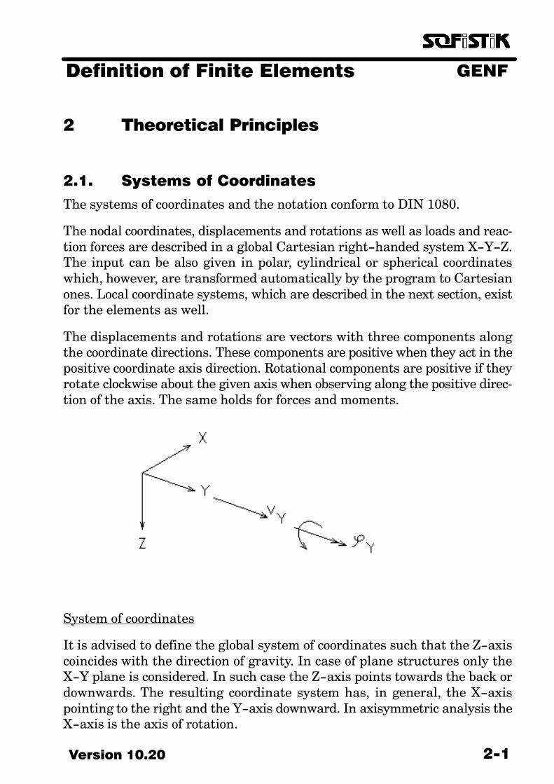
The displacements and rotations are vectors with three components alongthe coordinate directions. These components are positive when they act in thepositive coordinate axis direction. Rotational components are positive if theyrotate clockwise about the given axis when observing along the positive direc�tion of the axis. The same holds for forces and moments.
System of coordinates
It is advised to define the global system of coordinates such that the Z−axiscoincides with the direction of gravity. In case of plane structures only theX−Y plane is considered. In such case the Z−axis points towards the back ordownwards. The resulting coordinate system has, in general, the X−axispointing to the right and the Y−axis downward. In axisymmetric analysis theX−axis is the axis of rotation.
GENF Definition of Finite Elements
Version 10.202−2
2.2. Overview of the Element Types
2.2.1. Truss and Cable ElementsThe truss or cable element can only carry a constant axial force. In case of non�linear analysis, the cable element can not sustain any compression. The x−axis of the element direction is the only local coordinate axis.
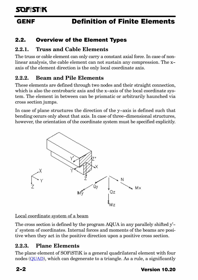
2.2.2. Beam and Pile ElementsThese elements are defined through two nodes and their straight connection,which is also the centrobaric axis and the x−axis of the local coordinate sys�tem. The element in between can be prismatic or arbitrarily haunched viacross section jumps.
In case of plane structures the direction of the y−axis is defined such thatbending occurs only about that axis. In case of three−dimensional structures,however, the orientation of the coordinate system must be specified explicitly.
Local coordinate system of a beam
The cross section is defined by the program AQUA in any parallely shifted y’−z’ system of coordinates. Internal forces and moments of the beams are posi�tive when they act in the positive direction upon a positive cross section.
2.2.3. Plane ElementsThe plane element of SOFiSTiK is a general quadrilateral element with fournodes (QUAD), which can degenerate to a triangle. As a rule, a significantly
GENFDefinition of Finite Elements
2−3Version 10.20
improved accuracy is achieved through non−conforming formulations, sothat the introduction of the problematic six− to nine− noded elements is notnecessary.
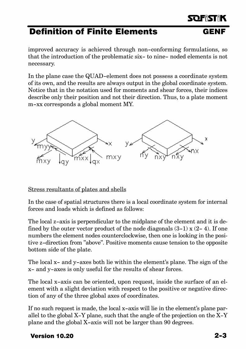
In the plane case the QUAD−element does not possess a coordinate systemof its own, and the results are always output in the global coordinate system.Notice that in the notation used for moments and shear forces, their indicesdescribe only their position and not their direction. Thus, to a plate momentm−xx corresponds a global moment MY.
Stress resultants of plates and shells
In the case of spatial structures there is a local coordinate system for internalforces and loads which is defined as follows:
The local z−axis is perpendicular to the midplane of the element and it is de�fined by the outer vector product of the node diagonals (3−1) x (2− 4). If onenumbers the element nodes counterclockwise, then one is looking in the posi�tive z−direction from "above". Positive moments cause tension to the oppositebottom side of the plate.
The local x− and y−axes both lie within the element’s plane. The sign of thex− and y−axes is only useful for the results of shear forces.
The local x−axis can be oriented, upon request, inside the surface of an el�ement with a slight deviation with respect to the positive or negative direc�tion of any of the three global axes of coordinates.
If no such request is made, the local x−axis will lie in the element’s plane par�allel to the global X−Y plane, such that the angle of the projection on the X−Yplane and the global X−axis will not be larger than 90 degrees.
GENF Definition of Finite Elements
Version 10.202−4
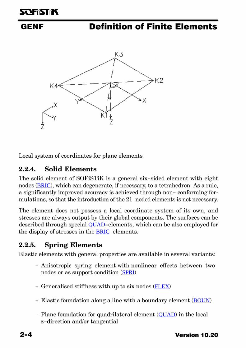
Local system of coordinates for plane elements
2.2.4. Solid ElementsThe solid element of SOFiSTiK is a general six−sided element with eightnodes (BRIC), which can degenerate, if necessary, to a tetrahedron. As a rule,a significantly improved accuracy is achieved through non− conforming for�mulations, so that the introduction of the 21−noded elements is not necessary.
The element does not possess a local coordinate system of its own, andstresses are always output by their global components. The surfaces can bedescribed through special QUAD−elements, which can be also employed forthe display of stresses in the BRIC−elements.
2.2.5. Spring ElementsElastic elements with general properties are available in several variants:
− Anisotropic spring element with nonlinear effects between twonodes or as support condition (SPRI)
− Generalised stiffness with up to six nodes (FLEX)
− Elastic foundation along a line with a boundary element (BOUN)
− Plane foundation for quadrilateral element (QUAD) in the localz−direction and/or tangential
GENFDefinition of Finite Elements
2−5Version 10.20
2.3. Mesh Partitioning
The partitioning of a mesh is specified based on two requirements. On onehand the mesh should be as fine as possible, so as to obtain the most accurateresults. The factors opposing that are:
− The computing times increase as n2, when the number of elementsn is increased.
− In case of very fine partitioning, roundoff errors are amplified somuch that the solution becomes unusable. As a rule of thumb, alogical partitioning of a free span consists of 5 up to 20 elements.
− It is not logical in construction practice to attempt to model andproportion all types of singularities. One should strive for a parti−tioning that is not too fine.
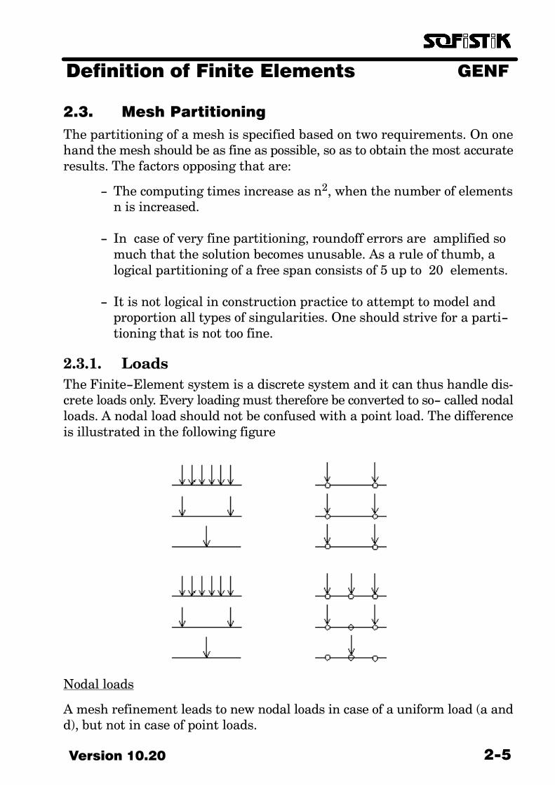
2.3.1. LoadsThe Finite−Element system is a discrete system and it can thus handle dis�crete loads only. Every loading must therefore be converted to so− called nodalloads. A nodal load should not be confused with a point load. The differenceis illustrated in the following figure
Nodal loads
A mesh refinement leads to new nodal loads in case of a uniform load (a andd), but not in case of point loads.
GENF Definition of Finite Elements
Version 10.202−6
On one hand, this means that a given mesh has a limited resolution for load�ings. The coarser mesh (a, b, c) can not make the differentiation between twopoint loads and a uniform load upon the element grid or a point load at themiddle of the element.
It also means on the other hand, that a loading can be applied as a point loadon a node only when its load induction area is smaller than the size of the ad�jacent elements. When inducing , for example, a point load upon a plate, eachnew mesh refinement in the area of the load will compute larger shear forceseach time, due to the better modelling of the singularity. Therefore, oneshould either select an element size that will not be smaller than the platethickness, or define the loads in the form of distributed loading with theiractual contact surfaces.
2.3.2. Beam ElementsAn exact description of the geometry is possible to a very large degree in thecase of beam elements. A single beam element may be used from one supportto the other. A typical FE partitioning of the geometry is necessary, however,in the following cases:
− Coupling with elastic foundation (Boundary element) − Dynamic computations (nodal masses) − Broken centrobaric axis (e.g. haunches) − Large deformations according to 3rd order theory
The partitioning may become so fine that the length of the individual beamswill approximately be the same as their cross section dimensions. When theirlength becomes smaller than that, it is required that the correct shear de�formation areas of the cross sections be input. Artificially large stiffnessesmust be avoided too, as well as the direct combination of elements with verydifferent lengths.
Results for this element can be obtained at all of its sections. Superposition�ing and proportioning can take place at these sections only.
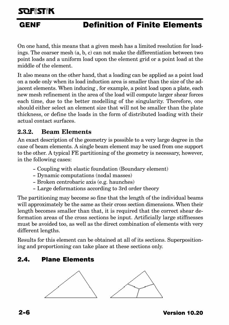
2.4. Plane Elements

GENFDefinition of Finite Elements
2−7Version 10.20
Conversion of triangular mesh to quadrilateral
This way for instance even a circular plate can be partitioned into quadrilat�eral elements easily:
Partitioning of a quarter−plate
Results for this element are obtained at the following points:
− At the centre of the element − At the so−called Gauss−points inside the element − As extrapolated average values of the nodes
The values at the element’s centre must be used for the proportioning of theelement. The so computed value of the required reinforcement must then beapplied to the entire area of the element. Through proper selection of the el�ement size and location, one can carry out direct calculations conforming tothe diverse dimensioning rules. It is meaningful e.g. in case of wide supportsor restraints, to place the centre of the element on top of the edge of the sup�port.
The Gauss−points are necessary only for an optimally accurate capture of theelements stress state and they are not usually employed by the user.
The values at the element nodes can be extrapolated from the Gauss− points.Due to the approximate formulation of the FEM−solution these values are notidentical at a node, therefore the average value is computed. These values areof prime importance for graphical representations. In case of coarse elementpartitioning, however, as well as in case of fixed edges or point supports thenodal values should be also taken into consideration in proportioning, be�cause otherwise the maximum values are not captured.
GENF Definition of Finite Elements
Version 10.202−8
Special care should be taken for three−dimensional structures or load ap�plication regions in order to avoid the averaging of all the stress resultantsat the nodes. In case of sudden changes in the element thickness as well, pro�portioning should take place, as a rule, separately on each side.
The nodal values can be also used in calculating an error indicator for theassessment of the accuracy of the solution, through the integration of thedeviations between extrapolated and average values for each element.
2.5. Solid Elements
Whatever was said for the QUAD−elements essentially holds for the solid el�ements as well.
2.6. Boundary Conditions
The boundary conditions at the nodes are specified in the simplest case bysuppressing the corresponding degrees of freedom. An elastic support is ob�tained by means of appropriate elements.
There is, however, a frequent need for special support conditions, which theengineer would like to model using infinitely large stiffnesses. Due to numeri�cal reasons the modelling should not be done with elements possessing verylarge stiffnesses, but with dependent degrees of freedom (kinematic con�straints) instead. The need for such constraints arises e.g. by oblique sup�ports or rigidly connected nodes. In general, every dependent degree of free�dom can be expressed as a linear combination of other displacements orrotations:
da� �� a1d1���a2d2��� ���
These conditions are taken into consideration explicitly in the assembly of theglobal stiffness matrix and, therefore, they are numerically more stable thanartificially rigid elements.
These combinations can be directly formulated by the record KINE and theycan become quite complex. However, the memory requirements for solving aproblem increase with the number of constraints and especially with thenumber of recursive associations.
Coupling conditions can be defined recursive up to 99 levels. Cyclic referencesor duplicate references are not possible.
GENFDefinition of Finite Elements
2−9Version 10.20
Standard conditions are available for the most frequent cases of constraintsin the form of the INTE record and the node coupling conditions.
Dependent degrees of freedom are designated by a * or a negative equationnumber in the node output. All displacements are always output, and theycomply to the specified dependencies. Reaction forces can be calculated viaECHO REAC for each node separately or in pairs for coupled nodes; in thelatter case they represent the force transmitted through the coupling.
Attention: Inappropriate use of couplings of the KINE type or the slave coup�lings (KPX through KPZ) may lead to mechanically absurd results (forcesmoved by couplings may violate the moment equilibrium).
2.6.1. Radial and Tangential SupportsA node can be supported in reference to some direction. By PR or MR, the dis�placement along or the rotation about this direction are, respectively, fixed;by PT or MT the respective displacement or rotation becomes the sole unre�stricted degree of freedom.
2.6.2. Rigid Body CouplingsThe couplings KP, KL, KQ and KF describe rigid bodies to which the depend�ent nodes are connected through a hinge (KP), or through a connection withfixed rotation about one (KQ), two (KL) or all three (KF) directions. One singleplane may be activated in special cases (KPEX, KPEY, KPEZ and KFEX,KFEY, KFEZ). This is, for instance, the case when defining a plane of thestructure which allows lateral bending but not in−plane distortion.
2.6.3. Symmetry ConditionsSymmetry conditions are a rarely needed special case of coupling. Conditionsof symmetry or anti−symmetry hold about the mid−perpendicular of the lineconnecting two nodes. In most cases the definition of a symmetry conditionis easier through the use of a lateral support. The direction of the supportmust then be perpendicular to the symmetry plane. PRMT defines a sym�metry and PTMR an anti−symmetry.
2.6.4. Eccentric ConnectionsEccentric connections, e.g. between a beam and a plate, can be specified byKF.
2.6.5. Slave SystemsA special class of couplings imposes the same displacements or rotations toseveral nodes (KPX to KMT). Their application is useful e.g. in the description
GENF Definition of Finite Elements
Version 10.202−10
of rigid foundation plates, which are not allowed to rotate. These couplingsact upon particular degrees of freedom and are thus more flexible. The dangeron the other hand is that their inappropriate use can produce undesired offsetmoments.
2.6.6. Mindlin Plate Boundary ConditionsThe formulation of the boundary conditions of plate elements is not uncriti�cal. The Mindlin−element especially has some peculiarities which should begiven attention.
According to Kirchhoff ’s theory two stress resultants exist on an edge,namely the bending moment and the equivalent shear force. The latter con�sists of the shear force and the torsional moment, and that is why both canhave values along a free edge different from zero. By contrast, Mindlin’stheory recognises three support conditions for the three stress−resultants i.e.bending moment, torsional moment and shear force. A support for the tor�sional moment, for example, suppresses the rotations perpendicular to theedge.
Free edges
Free edges do not have any constraints of any type. The reaction forces alongsuch edges are, within the bounds of computing accuracy, zero. The stress re�sultants inside the elements though are not always exactly zero, due to thenumerical method.
Fixed edges
Perfectly fixed edges can be input without any problems. For the interpreta�tion of the results, however, it is important to know, that the torsional reac�tion moments must be taken up. This takes place automatically in the outputof the BOUN−elements, where these are converted into corresponding sup�port loadings.
Simply supported edges
Here, one has a choice between the so−called soft support (only PZ) and thehard support (PZ+MT). In case of the soft support, shear deformations arestill allowed along the edge, and thus a shear force too; this can lead in somecases to considerable deviations from Kirchhoff ’s plate theory. On the otherhand, the soft support is more suitable for the manipulation of uplifting
GENFDefinition of Finite Elements
2−11Version 10.20
corners as well as of re−entrant corners. Particularly in the case of obtusecorners, the hard support leads to undesired fixing.
Simulation of support on masonry and concrete
There are generally four ways to describe such supports:
• Point− or line−supportThis type of support is mainly used for thin supports (width < platethickness). The size of the adjacent elements should be selected in sucha way that their gravity centre lies on the round section which is criti�cal for the punch−through check. The proportioning for the shear forcetakes place inside the element, whilst for the moment of the supportedside at the nodes of the support.
• Rotatable column head supportThe column is described through a node with fixed support and poss�ible rotational spring stiffness, which otherwise is not an elementnode. The column area is described by means of a single element aswell as coupling conditions between the four element nodes and the col�umn node, which specify that the cross section will remain plane with�out a restraint for the moment (KP for columns, KQ for walls). The sizeof the element can be between 2/3 of the column area (e.g. for circularcolumns) and the actual column area (e.g. by rectangular column crosssection). It goes with where one likes to arrange the resultant of the re�action pressure.The central element has a zero shear force and thus a uniform momentcorresponding to the moment of the section along the face of the col�umn. One should arrange additional elements for the shear forcecheck with their gravity centre lying on the round section used for thatcheck , or make a direct punch−through check.
• Elastic foundationThis variant is meaningful for elastic supports of large areas, for whicha rounded moment above the support is desired. The use of largefoundation coefficients (subgrade moduli), however, results into unde�sired restraints. The selection of the subgrade modulus is thus critical,and this variant should be applied to moderate foundations only.
• Special conditionsIn principle, any arbitrary conditions can be formulated through coup�lings. The effect though must be checked in every case.
GENF Definition of Finite Elements
Version 10.202−12
2.7. Girders
The modelling of girders in plate structures presents a special problem. Be�sides the option of modelling them with folded structure elements or solid el�ements, which is ruled out for practical processing, one has a choice betweentwo other options:
• The girder is modelled as a beam eccentrically connected to a planeshell (plate− and disk action). The area of the girder and its momentof inertia are determined from the protruding part of the girder.
For proportioning, the results of the shell and the beam should be com�bined into total stress resultants for a T−beam.
This method is general and always correct. It captures the co−operat�ing widths and their distribution in the structure.
• The girder is modelled as add−on element to a plate by defining allits cross sectional values (area, moment of inertia) as follows:
Add−on value = Total value of T−beam − contribution of co−operating part of plate
The total stiffness is correctly modelled in this manner. For propor�tioning girders with small heights one should always make construc�tive observations, as for instance assembling the individual values andapplying them to a T−beam cross section.
2.8. Literature
(1) O.C.Zienkiewicz (1984)Methode der finiten Elemente2. Auflage , Hanser Verlag München
(2) E.Ramm, J.Müller, K.WassermannProblemfälle bei FE−ModellierungenBaustatik, Baupraxis Tagung Hannover 1990
(3) C.Katz, J.StiedaPraktische FE−Berechnungen mit PlattenbalkenBauinformatik 3 (1992) Heft 1 S 30−34

GENFDefinition of Finite Elements
2−13Version 10.20
(4) M. GuptaError in Eccentric Beam FormulationInt.Journ.Num.Meth. in Engineering 11 (1977) 1473
(5) O.C.Zienkiewicz, ZhuA simple error estimate and adaptive procedure for practicalengineering analysis.Int.Journ.Num.Meth. in Engineering 24 (1987) 337−357
(6) C. KatzFehlerabschätzungen1. FEM−Tagung, Kaiserslautern 1989
2.9. Limitations
The following limits can not be exceeded in principle:
Number of cross sections: 999Number of nodes : 999 999Largest node number : 999 999Largest element number: 999 999Bore hole profiles : 999Hinge combinations : 10Segment definitions : 999
Each computer has a finite computing precision. This is normally 7 digits incase of 32 bits per word, and 15 digits in case of double precision. It is nat�urally meaningless to want to discuss about the 7. decimal digit of a final re�sult. The danger, however, is that in FE−analyses, as in most cases in real life,it is not the absolute size of a displacement that is of interest, but the differ�ences.
Because of that , all numerical calculations are sensitive to large variationsin stiffnesses or element dimensions, as well as to large numbers of elementsbetween two boundary conditions (supports).

GENFDefinition of Finite Elements
3−1Version 10.20
3 Input Description
The program GENF generates the basic structural system for plane or three−dimensional structures. On one hand the system consists of the nodes, de�fined by a number, their coordinates and geometric support conditions. Onthe other hand there are the elements, which are connected to each other atthese nodes.
The number and the type of the elements can not be changed subsequentlyduring a Restart of the program, whereas support conditions and materialparameters can be arbitrarily modified. Any input data that includes el�ements always defines a new system.
Cross sections are usually defined by the program AQUA. For purely staticanalysis though (without proportioning or state II stiffness), the cross sec�tions can be defined with GENF as well. Each cross section must have beendefined before an element can refer to it. Cross sectional data can be changedas often as the user likes, the latest input being valid at any time.
3.1. Nodes
Nodes are provided with a number for identification. Node numbers need notbe in a consecutive order. The maximum value of these numbers is limited to99999 due to the output format. In addition, since some of the programs workwith direct indices for quicker access, the highest possible node number iseventually limited by the available computer memory. The node numberinghas normally no influence on the bandwidth of the stiffness matrix becausethe system’s generation is directly combined with an optimisation of the pro�file and the bandwidth of the stiffness matrix. If this operation is suppressed,the bandwidth is directly determined by the node numbers as they were de�fined by the user. Nodes which are not used by any elements, do not have anyinfluence. Nodes can be defined as often as one likes, the last definition beingvalid at any time. Couplings, however, can not be defined more than once,when this would lead to a multiple dependency of the same degree of freedom.
3.2. Elements
Elements are also identified by an arbitrary number within the selected el�ement group. An element number though can be used only once for each el�

GENF Definition of Finite Elements
Version 10.203−2
ement type. Elements can be defined only once; if an element gets deleted, thesame element number can not be used any more.
The element number contains the group number. The latter is the integerpart of the element number divided by a freely defined divisor. The defaultvalue of this divisor GDIV by the record SYST is 99999, i.e. all elements areassigned to group 0. If the elements are subdivided into groups with a differ�ent value for GDIV, any elements of the group 0 that follow a group initiationby the record GRP are assigned to that group by their element number, i.e.the program changes the element numbers so as to adapt them to the activegroup.
Groups can be used in selecting a particular structural system or definingpartial regions for post−processing or graphical representation. A sensiblepartitioning of a structure into such groups can be very helpful in studyingstress resultants at nodes. In case of fold structures, one should arrange theelements of each disk into separate groups.
It is advantageous to number the elements in such a way that use can be madeof generation options during the system selection (groups) and the loadinginput (refer to STAR2, beam groups).
The theoretical background of the elements is described in the calculationprograms.
3.3. Results
The created structure is stored in the database (project file) and it can berepresented graphically by the program GRAF; this can be done even for er�ratic systems, so long as the program GENF has not terminated prematurelyafter the input. Further processing with other programs for analysis is poss�ible only when the structure is free of errors.
When no errors are detected, the structure’s data is output after being sorted,and a profile optimisation is performed on the stiffness matrix, in order to mi�nimise the cost of solving the system of equations for the structure at hand.
3.4. Restart
After a static or dynamic analysis, boundary conditions, material parametersand cross sections can be modified with Restart. Elements and nodal coordi�nates, however, remain unchanged. A restart takes place with the explicitinput SYST REST. The following can be included in a Restart input:
GENFDefinition of Finite Elements
3−3Version 10.20
− Nodes, yet only constraints without coordinates − Couplings − Material parameters and cross sections − Foundation profiles − Flexibility of particular node supports
It is stressed here that all couplings must be redefined, in case of couplinginput.
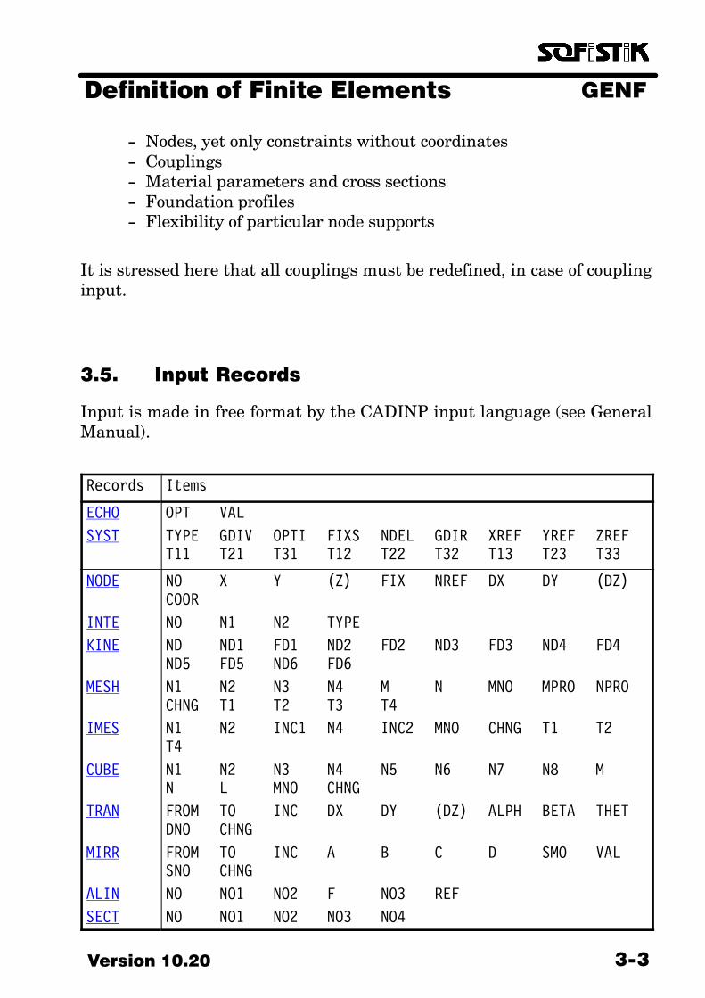
3.5. Input Records
Input is made in free format by the CADINP input language (see GeneralManual).
Records Items
ECHO
SYST
OPT VAL
TYPE GDIV OPTI FIXS NDEL GDIR XREF YREF ZREFT11 T21 T31 T12 T22 T32 T13 T23 T33
NODE
INTE
KINE
MESH
IMES
CUBE
TRAN
MIRR
ALIN
SECT
NO X Y (Z) FIX NREF DX DY (DZ)COOR
NO N1 N2 TYPE
ND ND1 FD1 ND2 FD2 ND3 FD3 ND4 FD4ND5 FD5 ND6 FD6
N1 N2 N3 N4 M N MNO MPRO NPROCHNG T1 T2 T3 T4
N1 N2 INC1 N4 INC2 MNO CHNG T1 T2T4
N1 N2 N3 N4 N5 N6 N7 N8 MN L MNO CHNG
FROM TO INC DX DY (DZ) ALPH BETA THETDNO CHNG
FROM TO INC A B C D SMO VALSNO CHNG
NO NO1 NO2 F NO3 REF
NO NO1 NO2 NO3 NO4

GENF Definition of Finite Elements
Version 10.203−4
Records Items
NORM
MAT
MATE
MLAY
BMAT
NMAT
MEXT
CONC
STEE
TIMB
BRWO
SSLA
DC NDC COUN
NO E MUE G K GAM GAMA ALFA EYMXY OAL OAF SPM TITL
NO E MUE G K GAM GAMA ALFA E90M90 OAL OAF SPM FY FT TITL
NO T0 NO0 T1 NO1 T2 NO2 T3 NO3T4 NO4 T5 NO5 T6 NO6 T7 NO7 T8NO8 T9 NO9 TITL
NO C CT CRAC YIEL MUE COH DIL GAMBREF MREF H
NO TYPE P1 P2 P3 P4 P5 P6 P7P8 P9 P10
NO TYPE VAL VAL1 VAL2 VAL3 VAL4 VAL5
NO TYPE FCN FC FCT FCTK EC QC GAMALFA SCM TYPR FCR GC GF MUEC TITL
NO TYPE CLAS FY FT FP ES QS GAMALFA SCM EPSY EPST REL1 REL2 R K1 FDYNTITL
NO TYPE CLAS EP G E90 QH QH90 GAMALFA SCM FM FT0 FT90 FC0 FC90 FV FVROAL OAF TITL
NO STYP SCLA MCLA E G MUE GAM ALFASCM FCN FC FT FHS FTB TITL
EPS SIG TYPE TEMP
BORE
BLAY
BBAX
BBLA
NO X Y Z NX NY NZ ALF TITL
S MNO ICEX MNOR ICRE HWMI HWMA
S1 S2 K0 K1 K2 K3 M0 C0 TANRTAND KSIG D0 D2
S1 S2 K0 K1 K2 K3 P0 P1 P2P3 PMA1 PMA2

GENFDefinition of Finite Elements
3−5Version 10.20
Records Items
SVAL
SREC
SCIR
HING
NO MNO A AY AZ IT IY IZ IYZCM YSC ZSC YMIN YMAX ZMIN ZMAX WT WVYWVZ NPL VYPL VZPL MTPL MYPL MZPL BCYZ TITL
NO H B HO BO SO SU ASO ASUMNO MRF ITF SAY SAZ DASO DASU REF TITL
NO RA RI SA SI ASA ASI MNO MRFITF DAS TITL
NO G1 G2 G3 G4 G5 G6
GRP NOG T MNO MRF STI NR POSI TX TYTXY TD
TRUS
CABL
BEAM
ADEF
BDIV
BSEC
SUPP
QUAD
BRIC
SPRI
BOUN
FLEX
DAMP
MASS
NO NA NE NCS PRE
NO NA NE NCS PRE
NO NA NE (NR) NCS AHIN EHIN DIV NBDNP NCSE
NO
DS NCS STYP PRIN DIRE LOC
NO X NCS STYP PRIN DIRE LOC
NO XFBM XSBM TYBM XFEM XSEM TYEM XFBT XSBTTYBT XFET XSET TYET TO INC
NO N1 N2 N3 N4 MNO DNO ENO NNOT C STI NR POSI CT MRF T1 T2T3 T4
NO N1 N2 N3 N4 N5 N6 N7 N8MNO
NO NA N2 DX DY DZ CP CT CMPRE GAP CRAC YIEL MUE COH DIL ENO DNONNO MNO AR
FROM TO INC TYPE CA CE REF RX RYRZ TITL
NO NO1 NO2 P VX VY VZ PHIX PHIYPHIZ PHIW
NO NA NE D DT DM
NO MX MY MZ MXX MYY MZZ MXY MXZMYZ REF
GENF Definition of Finite Elements
Version 10.203−6
The records can be input in any order; however, certain data (e.g. nodes) musthave been already introduced before any reference can be made to them (e.g.MESH). As an exception, the records ADEF and BDIV as well as BORE,BBAX and BBLA are meaningful only in a specific order.
The parameters between parentheses Z, DZ and NR are not applicable totwo−dimensional structures, therefore they are omitted from the input. Incase of the record NODE for a two−dimensional system, the parameter FIXmust be specified in the fourth place.
A description of each particular record follows.

GENFDefinition of Finite Elements
3−7Version 10.20
3.6. ECHO − Control of the Output
ÄÄÄÄÄÄÄÄÄÄÄÄÄÄÄÄÄÄÄÄÄÄÄÄÄÄÄÄÄÄÄÄ
ECHO
Item Description Dimension Default
OPT A literal from the following list:GEOD Geometric definitionsNODE Node parametersMAT Material propertiesGROU Group propertiesSECT Cross sectionsQUAD 2−D−elementsBRIC 3−D−elementsBEAM Flexible beams and pilesSPRI Spring elementsTRUS Truss−bar elementsCABL Cable elementsBOUN Boundary elementsSYST System values
FULL All the above options
NO Nothing printedPRIN Print despite any input errors
LIT FULL
VAL Output extentNO no outputYES regular output
LIT YES
The command name ECHO must always be repeated, otherwise confusionmay occur with other records with the same names (e.g. NODE).
The default value corresponds to regular output so long as the system hasbeen generated error free.

GENF Definition of Finite Elements
Version 10.203−8
See also: NODE
3.7. SYST − Global System
Parameters
ÄÄÄÄÄÄÄÄÄÄÄÄÄÄÄÄÄÄÄÄÄÄÄÄÄÄÄÄÄÄÄÄÄÄÄÄ
SYST
Item Description Dimension Default
TYPE FRAM Plane frame or disk(system lies in the XY−plane)
PAIN Plane strain conditionPESS Plane stress condition
(system lies in the XY−plane)AXIA Axisymmetric stress condition
(system lies in the XY−plane,rotation around x)
GIRD Gridwork or plate(system lies in the XY−plane)
SPAC Spatial frames or shells andfolded structures
REST Restart of the system withnew material and cross sec−tional properties or boundaryconditions
LIT FRAM
GENFDefinition of Finite Elements
3−9Version 10.20
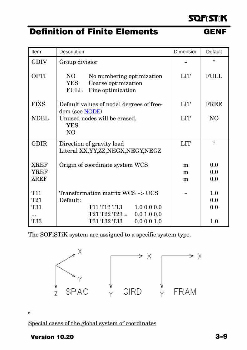
Item DefaultDimensionDescription
GDIV
OPTI
FIXS
NDEL
Group divisior
NO No numbering optimizationYES Coarse optimizationFULL Fine optimization
Default values of nodal degrees of free�dom (see NODE)Unused nodes will be erased.
YES NO
−
LIT
LIT
LIT
*
FULL
FREE
NO
GDIR
XREFYREFZREF
T11T21T31...T33
Direction of gravity loadLiteral XX,YY,ZZ,NEGX,NEGY,NEGZ
Origin of coordinate system WCS
Transformation matrix WCS −> UCSDefault:
T11 T12 T13 1.0 0.0 0.0T21 T22 T23 = 0.0 1.0 0.0T31 T32 T33 0.0 0.0 1.0
LIT
mmm
−
*
0.00.00.0
1.00.00.0
1.0
The SOFiSTiK system are assigned to a specific system type.
Special cases of the global system of coordinates

GENF Definition of Finite Elements
Version 10.203−10
It is advised to orientate the axes of coordinates so that the direction of grav�ity coincides with the z−axis for three−dimensional systems, with the y−axisfor FRAM systems and with the z−axis for GIRD systems. For some of the pro�grams (PILE, TALPA, ASE, ELSE) this orientation of the coordinate systemis mandatory.
XREF through T33 can be used in order to describe the position of the GENF−coordinate system relative to the world coordinate system WCS.
In the case of plane structures of the type FRAM/GIRD and/or PAIN/PESS/AXIA the output of out−of−plane deformations and stress−resultants is sup�pressed. Therefore, plane frames or gridworks, the axes of which do not co�incide with the principal axes of their cross sections, can be analyzed correctlyin three dimensions only.
Changes in an existing database (Restart) can be made by SYST REST. Thisis necessary for instance when changing the support conditions due to differ�ent construction stages. The type and number of the elements and their nodescan not be changed in such case.
The following can be defined in a Restart−input:
− Node constraints (no coordinates!), couplings− Material values and cross sections, foundation profiles− Flexibilities of individual nodes
Take notice that all couplings must be redefined, if any couplings are input.
Groups can be moved for the selection of a static system or for the definitionfrom subareas in case of evaluations or graphic representations here. In par�ticular can during the determination of internal forces and moments of nodesa reasonable group division be helpful. With folded structures itself is recom�mended to arrange the elements of the individual discs into separate groups.
The element number includes the group number implicit through the integralpart of the element number divided by a freely definable divisor. In the defaultthis divisor GDIV from sentence SYST has the value 99999, that is all el�ements are assigned to the group 0. If the elements are defined without anexplicit specificated value of the group (= group 0), than the elements follow�ing after a group inauguration with the sentence GRP are classified with theirelement number in this group. It means the element number is changed fromthe program in such a way that it is a part of the activ group.

GENFDefinition of Finite Elements
3−11Version 10.20
That one is preset from historical grounds temporarily still for data recordswithout every input to GRP formerly firm group divisor 1000. With that manydata records can be employed as before more further, and/or an only inputGRP suffices.
The volume width and/or the profile of the stiffness matrix has decisive influ�ence on the CPU time and the storage requirement to the solution of the Fi�nite−Element−system of equations. In the volume width and/or profile op�timization are minimized these sizes in a heuristic procedure. There thevolume width of the greatest difference in the FE−net occurring (intern, forthe user not visible) node numbers of an element derives, it is attempted toform the numbering so that neighboring nodes have numbers resting witheach other near. The quality of the volume width depends in this case also onthe choice of the start node.
In the ’standard optimization’ a probably well suitable node is chosen for thispurpose heuristically. In the expanded optimization is started (fundamental)from every node and preserved with that a i.a. better result, however, at theexpense of a larger CPU time for the optimization. This larger expenditurerewards for i.a., when during the following FE−calculation the system ofequations is very often to be solved (many loads, non−linear calculation) orboots onto the boundaries of the available CPU time or storeroom capacity,to itself then. Near the iterative equation solvers the volume width is neededonly for an estimate of the memory requirement.
OPTI NO must be input for partial structures not connected to each other.
GENF Definition of Finite Elements
Version 10.203−12
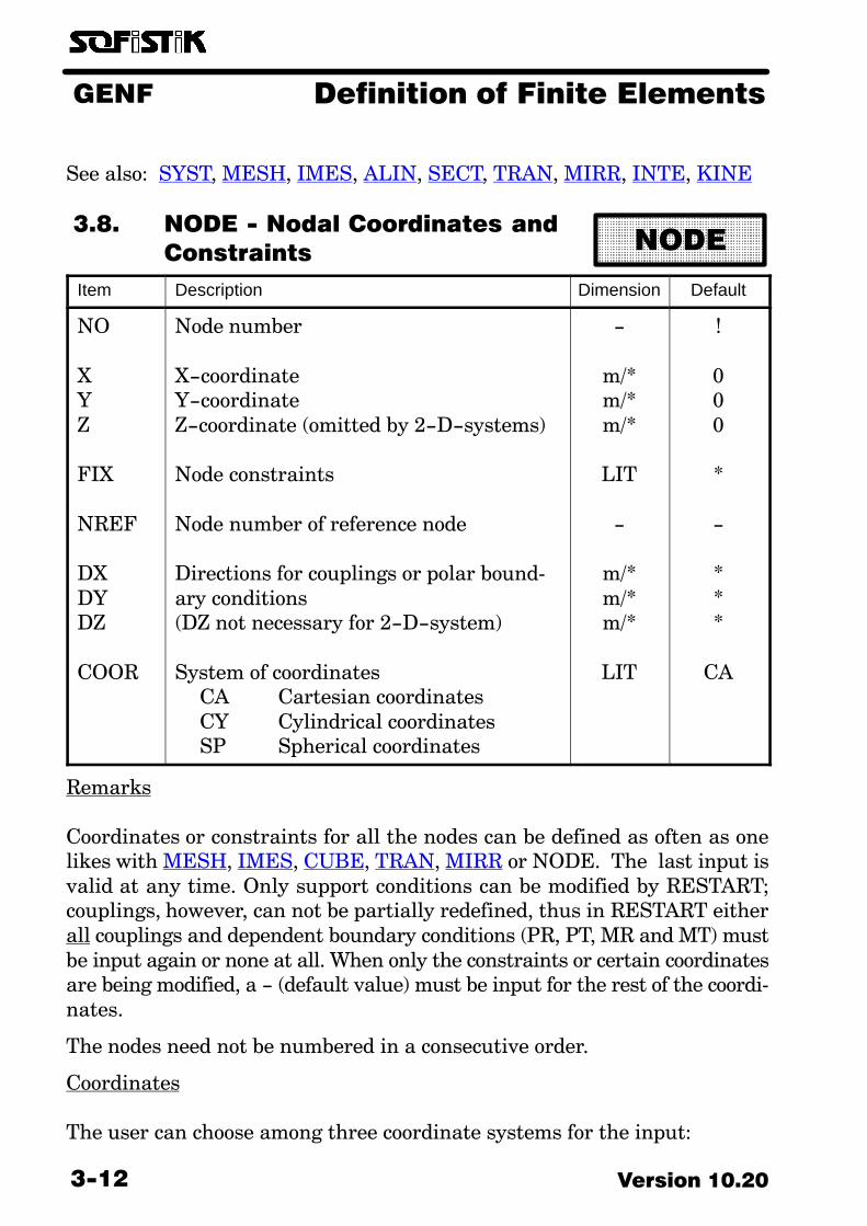
See also: SYST, MESH, IMES, ALIN, SECT, TRAN, MIRR, INTE, KINE
3.8. NODE − Nodal Coordinates and
Constraints
ÄÄÄÄÄÄÄÄÄÄÄÄÄÄÄÄÄÄÄÄÄÄÄÄÄÄÄ
NODE
Item Description Dimension Default
NO
XYZ
FIX
NREF
DXDYDZ
COOR
Node number
X−coordinateY−coordinateZ−coordinate (omitted by 2−D−systems)
Node constraints
Node number of reference node
Directions for couplings or polar bound�ary conditions(DZ not necessary for 2−D−system)
System of coordinatesCA Cartesian coordinatesCY Cylindrical coordinatesSP Spherical coordinates
−
m/*m/*m/*
LIT
−
m/*m/*m/*
LIT
!
000
*
−
***
CA
Remarks
Coordinates or constraints for all the nodes can be defined as often as onelikes with MESH, IMES, CUBE, TRAN, MIRR or NODE. The last input isvalid at any time. Only support conditions can be modified by RESTART;couplings, however, can not be partially redefined, thus in RESTART eitherall couplings and dependent boundary conditions (PR, PT, MR and MT) mustbe input again or none at all. When only the constraints or certain coordinatesare being modified, a − (default value) must be input for the rest of the coordi�nates.
The nodes need not be numbered in a consecutive order.
Coordinates
The user can choose among three coordinate systems for the input:
GENFDefinition of Finite Elements
3−13Version 10.20
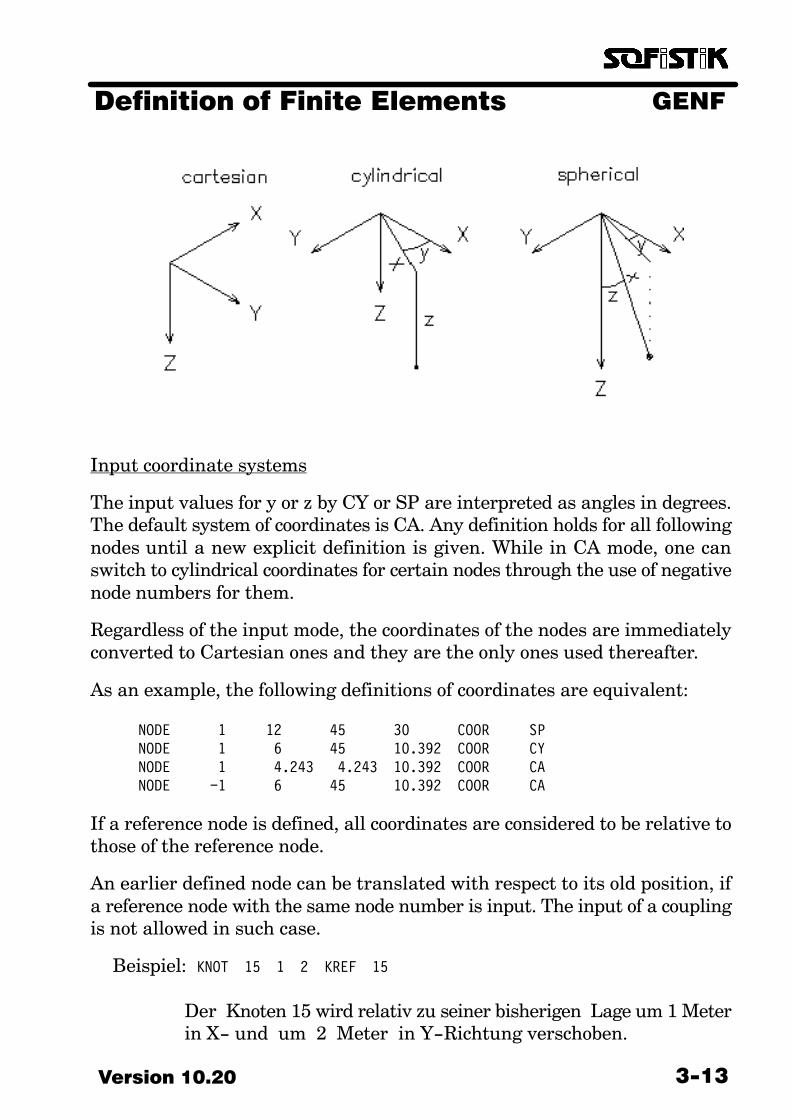
Input coordinate systems
The input values for y or z by CY or SP are interpreted as angles in degrees.The default system of coordinates is CA. Any definition holds for all followingnodes until a new explicit definition is given. While in CA mode, one canswitch to cylindrical coordinates for certain nodes through the use of negativenode numbers for them.
Regardless of the input mode, the coordinates of the nodes are immediatelyconverted to Cartesian ones and they are the only ones used thereafter.
As an example, the following definitions of coordinates are equivalent:
NODE 1 12 45 30 COOR SPNODE 1 6 45 10.392 COOR CYNODE 1 4.243 4.243 10.392 COOR CANODE −1 6 45 10.392 COOR CA
If a reference node is defined, all coordinates are considered to be relative tothose of the reference node.
An earlier defined node can be translated with respect to its old position, ifa reference node with the same node number is input. The input of a couplingis not allowed in such case.
Beispiel: KNOT 15 1 2 KREF 15
Der Knoten 15 wird relativ zu seiner bisherigen Lage um 1 Meterin X− und um 2 Meter in Y−Richtung verschoben.

GENF Definition of Finite Elements
Version 10.203−14
Example: NODE 15 1 2 NREF 15
Node 15 is translated 1 m in the X− and 2 m in the Y−direction withrespect to its previous position.
It is impossible to specify couplings to a reference node and absolute coordi�nates in the same record. It is best, in principle, first to define all the nodalcoordinates and then all the couplings (without coordinates).
Nodal constraints
All the constraints of a node can be described by any combination of the follow�ing literals (limited up to 8 characters). Any degree of freedom not includedin a 2−D system gets fixed. The default constraint is the value defined byFIXS in SYST.
PX Constraint of displacement in xPY Constraint of displacement in yPZ Constraint of displacement in zPR Constraint of radial displacementPT Constraint of tangential displacement
MX Contstraint of rotation about xMY Contstraint of rotation about yMZ Contstraint of rotation about zMR Contstraint of rotation about radial directionMT Contstraint of rotation about tangential directionMB Constraint of warping
XP = PY + PZYP = PX + PZZP = PX + PYPP = PX + PY + PZ
XM = MY + MZYM = MX + MZZM = MX + MYMM = MX + MY + MZ + MB
FREE = Deletion of all constraintsF = PP + MM
GENFDefinition of Finite Elements
3−15Version 10.20
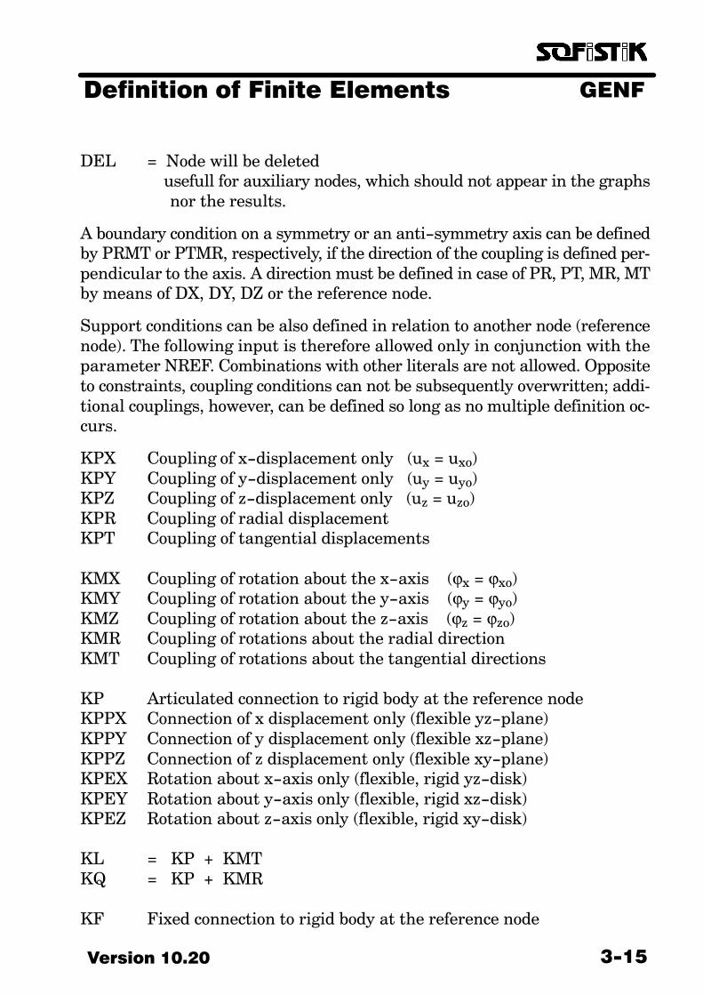
DEL = Node will be deleted usefull for auxiliary nodes, which should not appear in the graphs nor the results.
A boundary condition on a symmetry or an anti−symmetry axis can be definedby PRMT or PTMR, respectively, if the direction of the coupling is defined per�pendicular to the axis. A direction must be defined in case of PR, PT, MR, MTby means of DX, DY, DZ or the reference node.
Support conditions can be also defined in relation to another node (referencenode). The following input is therefore allowed only in conjunction with theparameter NREF. Combinations with other literals are not allowed. Oppositeto constraints, coupling conditions can not be subsequently overwritten; addi�tional couplings, however, can be defined so long as no multiple definition oc�curs.
KPX Coupling of x−displacement only (ux = uxo)KPY Coupling of y−displacement only (uy = uyo)KPZ Coupling of z−displacement only (uz = uzo)KPR Coupling of radial displacementKPT Coupling of tangential displacements
KMX Coupling of rotation about the x−axis (ϕx = ϕxo)KMY Coupling of rotation about the y−axis (ϕy = ϕyo)KMZ Coupling of rotation about the z−axis (ϕz = ϕzo)KMR Coupling of rotations about the radial directionKMT Coupling of rotations about the tangential directions
KP Articulated connection to rigid body at the reference nodeKPPX Connection of x displacement only (flexible yz−plane)KPPY Connection of y displacement only (flexible xz−plane)KPPZ Connection of z displacement only (flexible xy−plane)KPEX Rotation about x−axis only (flexible, rigid yz−disk)KPEY Rotation about y−axis only (flexible, rigid xz−disk)KPEZ Rotation about z−axis only (flexible, rigid xy−disk)
KL = KP + KMTKQ = KP + KMR
KF Fixed connection to rigid body at the reference node
GENF Definition of Finite Elements
Version 10.203−16
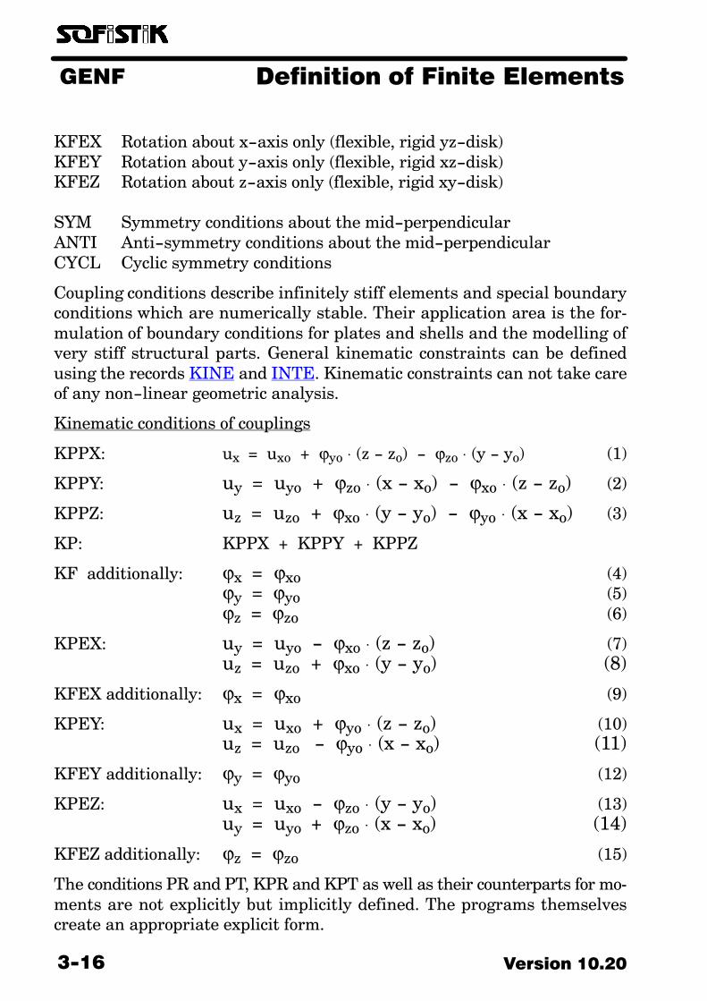
KFEX Rotation about x−axis only (flexible, rigid yz−disk)KFEY Rotation about y−axis only (flexible, rigid xz−disk)KFEZ Rotation about z−axis only (flexible, rigid xy−disk)
SYM Symmetry conditions about the mid−perpendicularANTI Anti−symmetry conditions about the mid−perpendicularCYCL Cyclic symmetry conditions
Coupling conditions describe infinitely stiff elements and special boundaryconditions which are numerically stable. Their application area is the for�mulation of boundary conditions for plates and shells and the modelling ofvery stiff structural parts. General kinematic constraints can be definedusing the records KINE and INTE. Kinematic constraints can not take careof any non−linear geometric analysis.
Kinematic conditions of couplings
KPPX: ux = uxo + ϕyo ⋅ (z − zo) − ϕzo ⋅ (y − yo) (1)
KPPY: uy = uyo + ϕzo ⋅ (x − xo) − ϕxo ⋅ (z − zo) (2)
KPPZ: uz = uzo + ϕxo ⋅ (y − yo) − ϕyo ⋅ (x − xo) (3)
KP: KPPX + KPPY + KPPZ
KF additionally: ϕx = ϕxo (4)ϕy = ϕyo (5)ϕz = ϕzo (6)
KPEX: uy = uyo − ϕxo ⋅ (z − zo) (7)uz = uzo + ϕxo ⋅ (y − yo) (8)
KFEX additionally: ϕx = ϕxo (9)
KPEY: ux = uxo + ϕyo ⋅ (z − zo) (10)uz = uzo − ϕyo ⋅ (x − xo) (11)
KFEY additionally: ϕy = ϕyo (12)
KPEZ: ux = uxo − ϕzo ⋅ (y − yo) (13)uy = uyo + ϕzo ⋅ (x − xo) (14)
KFEZ additionally: ϕz = ϕzo (15)
The conditions PR and PT, KPR and KPT as well as their counterparts for mo�ments are not explicitly but implicitly defined. The programs themselvescreate an appropriate explicit form.

GENFDefinition of Finite Elements
3−17Version 10.20
PR: ut ⋅ n = 0ux ⋅ dx + uy ⋅ dy + uz ⋅ dz = 0 (16)
PT: u ⋅ n = 0
uxdx
� ��uy
dy��� uz
dz(17)
KPR: (u−uo)t ⋅ n = 0(ux−uxo)⋅dx + (uy−uyo)⋅dy + (uz−uzo)⋅dz = 0 (18)
KPT: (u−uo) ⋅ n = 0
(ux�uxo)
dx� ��
�uy�uyo�dy
� ��(uz�uzo)
dz (19)
The symmetry and anti−symmetry conditions are given in the followingequations in vectorial form. A presentation by their components is not in�cluded here:
SYM: ut ⋅ n = − uto ⋅ n
ANTI: ut ⋅ n = uto ⋅ n
The directional or differential vector n = (dx,dy,dz) is built from the differ�ences of the node coordinates. These coordinate differences can also be speci�fied explicitly by means of DX, DY and DZ.
Certain degrees of freedom that have been coupled can be constrained againwith input of a constraint after the coupling condition.

GENF Definition of Finite Elements
Version 10.203−18
See also: KINE, NODE
3.9. INTE − Intermediate Nodes
ÄÄÄÄÄÄÄÄÄÄÄÄÄÄÄÄÄÄÄÄÄÄÄÄÄÄÄÄÄÄÄÄÄÄÄÄ
INTE
Item Description Dimension Default
NON1N2
TYPE
Number of intermediate nodeNumber of a corner nodeNumber of a corner node
Type of InterpolationP Linear displacementsF Linear displacements +
constant rotationsQ Quadratic displacements +
linear rotations
−−−
LIT
!!!
F
In case of mesh refinement or in cases of stiff cross−girders there may arisea need for nodes that lie between two others and depend on them. This kindof dependency can be described by INTE.
INTE−couplings
The INTE−coupling is a constraint with special attributes. Herein, oppositeto node couplings, one node (the middle node) becomes dependent on twoother nodes. The displacements and rotations of the middle node are interpo�lated from the corresponding ones of the adjacent nodes.

GENFDefinition of Finite Elements
3−19Version 10.20
u0 = u1 · DD + u2 · (1−DD)
When the deflections of the outer nodes are somehow prescribed, e.g. fixed orprovided with a certain stiffness, the deflection of the middle node is pre�scribed in the same way too. The coupling is rigid only when both nodes cannot displace relatively to each other. A rigid body with three nodes must bedescribed by means of two KP/KF couplings; the INTE−coupling can not beused in that case.
There are several variants of interpolation used by INTE−couplings, whichare described in the following.
TYPE P Displacements: linearly interpolatedRotations: not definedApplication: mesh refinements TALPA
TYPE FDisplacements: linearly interpolated as in TYPE PRotations: �torsion" linearly interpolated, other rotations com−
puted from displacement differences divided by therespective node distances
Application: connection of beam elements onto disksstiff cross−girders between two supports
In the general three−dimensional case, if one draws the lines connecting thetwo nodes in the initial undeformed as well as in their deformed state, tworotational components are defined exactly by the secant angles of those. Thethird yet undetermined rotational component has the direction of the con�necting line (torsion), and it is normally interpolated. The general expressionis very complicated; however, INTE−couplings parallel to the axes of coordi�nates can be expressed by much simpler expressions, e.g.,
DX = 0.DY = dDZ = 0.
results in:
ϕx = � uz / d
ϕy = ϕy−m
GENF Definition of Finite Elements
Version 10.203−20
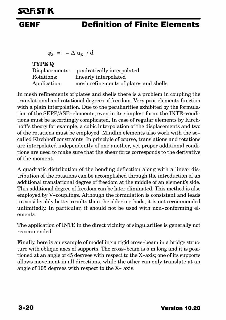
ϕz = − � ux / d
TYPE QDisplacements: quadratically interpolatedRotations: linearly interpolatedApplication: mesh refinements of plates and shells
In mesh refinements of plates and shells there is a problem in coupling thetranslational and rotational degrees of freedom. Very poor elements functionwith a plain interpolation. Due to the peculiarities exhibited by the formula�tion of the SEPP/ASE−elements, even in its simplest form, the INTE−condi�tions must be accordingly complicated. In case of regular elements by Kirch�hoff ’s theory for example, a cubic interpolation of the displacements and twoof the rotations must be employed. Mindlin elements also work with the so−called Kirchhoff constraints. In principle of course, translations and rotationsare interpolated independently of one another, yet proper additional condi�tions are used to make sure that the shear force corresponds to the derivativeof the moment.
A quadratic distribution of the bending deflection along with a linear dis�tribution of the rotations can be accomplished through the introduction of anadditional translational degree of freedom at the middle of an element’s side.This additional degree of freedom can be later eliminated. This method is alsoemployed by V−couplings. Although the formulation is consistent and leadsto considerably better results than the older methods, it is not recommendedunlimitedly. In particular, it should not be used with non−conforming el�ements.
The application of INTE in the direct vicinity of singularities is generally notrecommended.
Finally, here is an example of modelling a rigid cross−beam in a bridge struc�ture with oblique axes of supports. The cross−beam is 5 m long and it is posi�tioned at an angle of 45 degrees with respect to the X−axis; one of its supportsallows movement in all directions, while the other can only translate at anangle of 105 degrees with respect to the X− axis.

GENFDefinition of Finite Elements
3−21Version 10.20
NODE 1 0.0 0.0 FIX PTMM DX COS(105) DY SIN(105)NODE −3 5.0 45 FIX KPR 1 ; 3 FIX PZMT DX 1 DY 1NODE −2 2.5 45 ; INTE 2 1 3 TYPE F
The constraint PT determines the translational freedom. The two perpen�dicular directions as well as Z are fixed. MM is important, so that no movablesystem results. Node 3 is defined in polar mode with respect to 1. KPR definesa fixed distance. The constraint PZ overwrites here part of the coupling, thusit must certainly come after that. MT on the other hand does not conflict withKPR, therefore it could have been input earlier as well. Node 3 can now moveonly in a circle about node 1 in the X−Y plane. The constraint MM of node 1has no influence on that. Node 2 which is defined by INTE has now all its de�grees of freedom defined. It is still free to rotate about the 1−3 axis throughthe MT constraint of node 3. A fixed support condition could have been definedby MM on node 3.

GENF Definition of Finite Elements
Version 10.203−22
See also: INTE, NODE
3.10. KINE − Kinematic
DependenciesÄÄÄÄÄÄÄÄÄÄÄÄÄÄÄÄÄÄÄÄÄÄÄÄÄÄÄ
KINE
Item Description Dimension Default
ND
ND1FD1ND2FD2......ND6FD6
Dependent degree of freedom
Reference degree of freedom 1Factor for reference degree of freedom 1
LIT
LIT
!
−−
In special cases kinematic dependencies can be described explicitly too:
(ND) = (ND1) · FD1 + ..... + (ND6) · FD6
The degrees of freedom are defined by:
nodenumber · 10 + local degree of freedom
1 = ux 2 = uy 3 = uz4 = ϕx 5 = ϕy 6 = ϕz
e.g the record
KINE 1003 13 1.0 25 0.5
means that the displacement uz of node 100 is prescribed to be the sum of thedisplacement uz of node 1 and one−half of the rotation ϕy of node 2.
If a positive number is entered for ND, the same coupling holds for the reac�tion forces too. Therefore, no reaction forces arise at coupled nodes. If ND isnegative, however, the coupling holds for the displacements only. Rigid bodiesare typical cases of the first variant, oblique supports are typical of the secondone.
GENFDefinition of Finite Elements
3−23Version 10.20
See also: IMES, CUBE, NODE, GRP
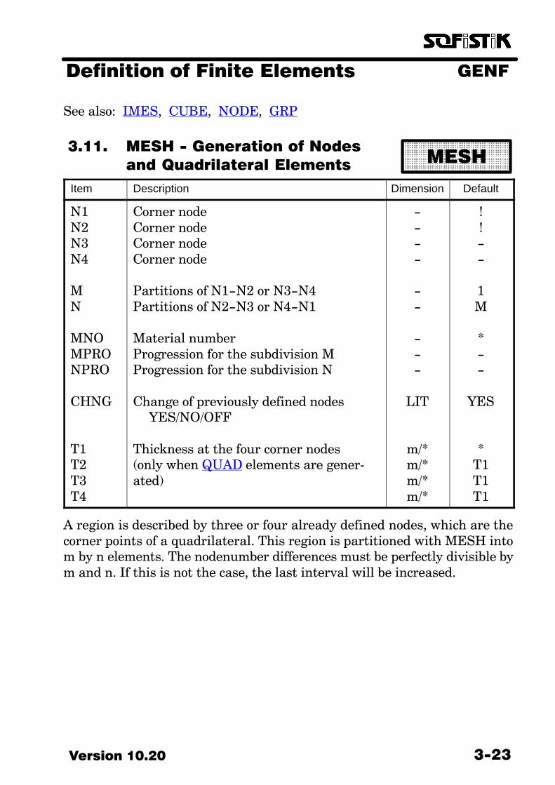
3.11. MESH − Generation of Nodes
and Quadrilateral Elements
ÄÄÄÄÄÄÄÄÄÄÄÄÄÄÄÄÄÄÄÄÄÄÄÄÄÄÄÄÄÄÄÄ
MESH
Item Description Dimension Default
N1N2N3N4
MN
MNOMPRONPRO
CHNG
T1T2T3T4
Corner nodeCorner nodeCorner nodeCorner node
Partitions of N1−N2 or N3−N4Partitions of N2−N3 or N4−N1
Material numberProgression for the subdivision MProgression for the subdivision N
Change of previously defined nodesYES/NO/OFF
Thickness at the four corner nodes(only when QUAD elements are gener�ated)
−−−−
−−
−−−
LIT
m/*m/*m/*m/*
!!−−
1M
*−−
YES
*T1T1T1
A region is described by three or four already defined nodes, which are thecorner points of a quadrilateral. This region is partitioned with MESH intom by n elements. The nodenumber differences must be perfectly divisible bym and n. If this is not the case, the last interval will be increased.

GENF Definition of Finite Elements
Version 10.203−24
MESH−generation
Remark
The number assigned to the elements is the node number of the corner nodeoriented towards N1. In case a record of the GRP type has been previouslyinput (or GDIV in record SYST), the numbers get changed appropriately.
The default value for MNO can be set by a preceding GRP record. If a negativeMNO is input, the elements are not assigned the number of the correspondingN1 corner node, instead they are numbered consecutively in the active groupNOG of the GRP record. The first element of the mesh is assigned the numberGDIV * NOG + 1. The group divisor is defined in the record SYST.
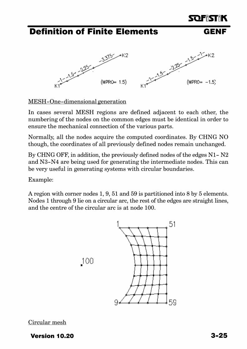
Regions with partitions varying like geometric progressions can be definedby MPRO or NPRO. Beginning from side N4−N1, each segment is MPROtimes the previous one. If MPRO is negative, a symmetric partitioning takesplace (length of first segment equal to that of the last one).
Recesses can be defined afterwards with QUAD. Node constraints are not af�fected by MESH.
If only N1, N2, M and possibly MPRO are given, then only nodes on the lineconnecting N1 and N2 will be generated.
GENFDefinition of Finite Elements
3−25Version 10.20
MESH−One−dimensional generation
In cases several MESH regions are defined adjacent to each other, thenumbering of the nodes on the common edges must be identical in order toensure the mechanical connection of the various parts.
Normally, all the nodes acquire the computed coordinates. By CHNG NOthough, the coordinates of all previously defined nodes remain unchanged.
By CHNG OFF, in addition, the previously defined nodes of the edges N1− N2and N3−N4 are being used for generating the intermediate nodes. This canbe very useful in generating systems with circular boundaries.
Example:
A region with corner nodes 1, 9, 51 and 59 is partitioned into 8 by 5 elements.Nodes 1 through 9 lie on a circular arc, the rest of the edges are straight lines,and the centre of the circular arc is at node 100.
Circular mesh

GENF Definition of Finite Elements
Version 10.203−26
$ CIRCLE CENTERNODE 100 −4.00 0.00 FIX F$ POLAR COORDINATES N1−N2NODE (−1 −9 −1) 4.00*SQR(2) (−45 11.25) NREF 100$ CORNER NODESNODE 51 5.00 −4.00NODE 59 5.00 4.00MESH 1 9 59 51 M 8 5 MNO 1 CHNG OFF
GENFDefinition of Finite Elements
3−27Version 10.20
See also: MESH, CUBE, NODE, GRP
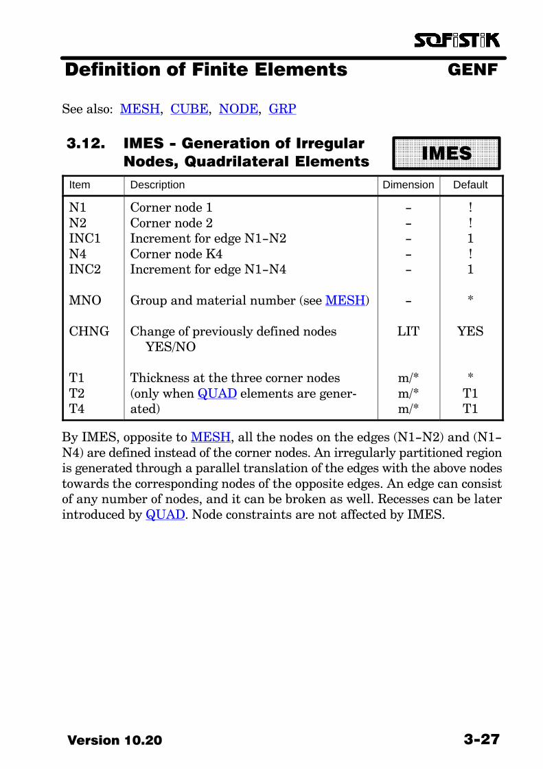
3.12. IMES − Generation of Irregular
Nodes, Quadrilateral Elements
ÄÄÄÄÄÄÄÄÄÄÄÄÄÄÄÄÄÄÄÄÄÄÄÄÄÄÄÄÄÄÄÄ
IMES
Item Description Dimension Default
N1N2INC1N4INC2
MNO
CHNG
T1T2T4
Corner node 1Corner node 2Increment for edge N1−N2Corner node K4Increment for edge N1−N4
Group and material number (see MESH)
Change of previously defined nodesYES/NO
Thickness at the three corner nodes(only when QUAD elements are gener�ated)
−−−−−
−
LIT
m/*m/*m/*
!!1!1
*
YES
*T1T1
By IMES, opposite to MESH, all the nodes on the edges (N1−N2) and (N1−N4) are defined instead of the corner nodes. An irregularly partitioned regionis generated through a parallel translation of the edges with the above nodestowards the corresponding nodes of the opposite edges. An edge can consistof any number of nodes, and it can be broken as well. Recesses can be laterintroduced by QUAD. Node constraints are not affected by IMES.

GENF Definition of Finite Elements
Version 10.203−28
IMES−generation

GENFDefinition of Finite Elements
3−29Version 10.20
See also: MESH, IMES, NODE
3.13. CUBE − Nodes and Cubic
Elements
ÄÄÄÄÄÄÄÄÄÄÄÄÄÄÄÄÄÄÄÄÄÄÄÄÄÄÄÄÄÄÄÄ
CUBE
Item Description Dimension Default
N1N2N3N4N5N6N7N8
M
N
L
MNO
CHNG
Corner nodeCorner nodeCorner nodeCorner nodeCorner nodeCorner nodeCorner nodeCorner node
Partitions of N1−N2, N3−N4, N5−N6,N7−N8Partitions of N2−N3, N4−N1, N6−N7,N8−N5Partitions of N1−N5, N2−N6, N3−N7,N4−N8
Group and material number (see MESH)
Change of previously defined nodesYES/NO
−−−−−−−−
−
−
−
−
LIT
!!!!!!!!
1
M
M
*
YES
Nodes N1 through N8 are the corner nodes of an 8−cornered solid region. Thisregion is subdivided by CUBE into L by M by N elements. The differences(N1−N2), (N3−N4), (N5−N6) and (N7−N8) must be divisible by M; similarlyfor N and L. Recesses can be defined later on by the BRIC record. Node con�straints are not affected by CUBE.

GENF Definition of Finite Elements
Version 10.203−30
CUBE−generation
GENFDefinition of Finite Elements
3−31Version 10.20
See also: MIRR, ALIN, SECT, NODE
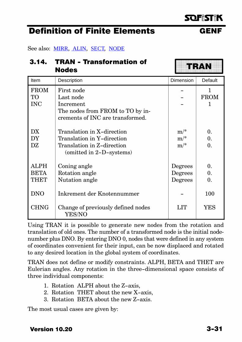
3.14. TRAN − Transformation of
Nodes
ÄÄÄÄÄÄÄÄÄÄÄÄÄÄÄÄÄÄÄÄÄÄÄÄ
TRAN
Item Description Dimension Default
FROMTOINC
DXDYDZ
ALPHBETATHET
DNO
CHNG
First nodeLast nodeIncrementThe nodes from FROM to TO by in�crements of INC are transformed.
Translation in X−directionTranslation in Y−directionTranslation in Z−direction
(omitted in 2−D−systems)
Coning angleRotation angleNutation angle
Inkrement der Knotennummer
Change of previously defined nodesYES/NO
−−−
m/*m/*m/*
DegreesDegreesDegrees
−
LIT
1FROM
1
0.0.0.
0.0.0.
100
YES
Using TRAN it is possible to generate new nodes from the rotation andtranslation of old ones. The number of a transformed node is the initial node�number plus DNO. By entering DNO 0, nodes that were defined in any systemof coordinates convenient for their input, can be now displaced and rotatedto any desired location in the global system of coordinates.
TRAN does not define or modify constraints. ALPH, BETA and THET areEulerian angles. Any rotation in the three−dimensional space consists ofthree individual components:
1. Rotation ALPH about the Z−axis,2. Rotation THET about the new X−axis,3. Rotation BETA about the new Z−axis.
The most usual cases are given by:

GENF Definition of Finite Elements
Version 10.203−32
ALPH: BETA: THET:0 0 phi : Rotation about the X−axis
90 −90 phi : Rotation about the Y−axis0 phi 0 : Rotation about the Z−axis
Only the angle BETA and the displacements DX, DY are used in plane cases.

GENFDefinition of Finite Elements
3−33Version 10.20
See also: TRAN, ALIN, SECT, NODE
3.15. MIRR − Mirroring of Nodes
ÄÄÄÄÄÄÄÄÄÄÄÄÄÄÄÄÄÄÄÄÄÄÄÄÄÄÄÄÄÄÄÄ
MIRR
Item Description Dimension Default
FROMTOINC
ABCD
SMO
VAL
SNO
CHNG
First nodeLast nodeIncrementThe nodes from FROM to TO by incre−ments of INC are mirrored.
Constants defining the plane of mirror�ing by
A⋅x + B⋅y + C⋅z + D = 0.
Partition point of node number
Transformation for new node numberSV Mirroring of primary numberSN Mirroring of secondary
numberAV Addition of primary numberAN Addition of secondary numberT Interchange of primary and
secondary numbers
Number for mirroring or addition
Change of previously defined nodesYES/NO
−−−
−
−
LIT
−
LIT
1FROM
1
0.
2
SV
100
YES
Using MIRR one can generate new nodes from the mirroring of other alreadyexisting nodes. Constraints can neither be set nor changed by MIRR.
The procedure for calculating the new node number is relatively complicatedin order to account for all possible cases. To begin with, the node number ispartitioned into the so−called primary and secondary number. The point ofpartition is specified by SMO. The secondary number is defined by as many
GENF Definition of Finite Elements
Version 10.203−34
of the last digits as SMO, while the primary number is built by the rest of thedigits at the beginning of the node number.
The mirror of a number is defined as:
NO NEW = SNO + (SNO − NO OLD)
SNO can also differ from a whole number by 1/2.
The user now has a choice among several transformation options:
By SV or SN the primary or secondary part of the old node number, respect�ively, will be mirrored with respect to SNO, whilst by AV or AN, SNO will beadded to the primary or secondary part of the old node number, respectively.
Example : Nodenumber 723, with SMO=2 and SNO=50Primary number 07, Secondary number 23
is transformed by mirroring of the primary number to: 9323by mirroring of the secondary number to: 777by addition to primary number to: 5723by addition to secondary number to: 773by interchange to: 2307
The range FROM TO must define as exactly as possible the range of the mir�rored nodes, so that the generated nodes lie in the permissible range for nodenumbers. As a rule, an input with TO = 9999 does not satisfy this require�ment.
S: y = yo B = 1.0D = −yo

GENFDefinition of Finite Elements
3−35Version 10.20
Mirror plane

GENF Definition of Finite Elements
Version 10.203−36
See also: SECT, MIRR, TRAN, NODE
3.16. ALIN − Node upon a Line
(Projection to the Line)
ÄÄÄÄÄÄÄÄÄÄÄÄÄÄÄÄÄÄÄÄÄÄÄÄÄÄÄÄÄÄÄÄÄÄÄÄ
ALIN
Item Description Dimension Default
NO
NO1NO2FNO3
REF
Node number
Node at the beginning of the lineNode at the end of the lineDistance of node from node 1 Node away from the line
Reference system for F
−
−−−−
LIT
!
!!−
NO
SS
Using ALIN one can define a node on the straight line connecting two otheralready defined nodes. With the same record an already existing node can beprojected onto that line.
ALIN−intermediate nodes
Generally there are two possibilities for the generation of nodes on a line:
1. Specification of a distance on a a line from a point (item F)2. Definition of the position with a auxiliary point (item NO3)
In the first case the item F which describes the distance of the new node tothe node NO1 has to be defined. The auxiliary point number is input with the

GENFDefinition of Finite Elements
3−37Version 10.20
item NO3 in the second case. Thus either a numerical value for F or a nodenumber for NO3 can be specified.
The new point has to be defined with an input of S,SS for REF directly on theline or on the auxiliary line. The input of a literal consisting of two same al�phabetic characters for REF ( e.g. XX, YY, ZZ) describes the definition of a ref�erence axis. However, the input of a literal consisting of two different alpha�betic characters (e.g. XY, YZ, XZ) defines a reference plane.
1. Input of F
REF Meaning
SXXYYZZ
XYXZYZ
SS
F in m on the straight line NO1 − NO2 F in m on the projection of the line onto global x−axisF in m on the projection of the line onto global y−axisF in m on the projection of the line onto global z−axis
F in m on the projection of the line onto global xy−planeF in m on the projection of the line onto global xz−planeF in m on the projection of the line onto global yz−plane
dimensionless 0 − 1 The node lies at NO1 + F ⋅ [NO2 − NO1]
In case of S, the distance along the true length of the straight line from NOto NO1 is input.
In case of XX, YY or ZZ, only the components along the respective axes areinput. F 2.0 REF YY means, for example, that the Y−coordinate of NO islarger than the one of NO1 by 2.0. The missing coordinates result from thecondition that NO lies upon the connecting straight line.
In case of XY, XZ or YZ, the two coordinates are used together. In case of XY,for example, the distance in top view is input. The ratio as well as the missingZ−coordinate are again deduced from the connecting line.
Lastly, SS defines a dimensionless input. 0.5 e.g. stands for a point exactly atthe middle between NO1 and NO2.
2. Input of NO3
GENF Definition of Finite Elements
Version 10.203−38
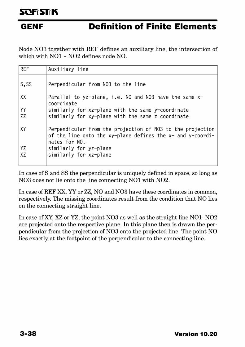
Node NO3 together with REF defines an auxiliary line, the intersection ofwhich with NO1 − NO2 defines node NO.
REF Auxiliary line
S,SS
XX
YYZZ
XY
YZXZ
Perpendicular from NO3 to the line
Parallel to yz−plane, i.e. NO and NO3 have the same x−coordinatesimilarly for xz−plane with the same y−coordinate similarly for xy−plane with the same z coordinate
Perpendicular from the projection of NO3 to the projectionof the line onto the xy−plane defines the x− and y−coordi−nates for NO.similarly for yz−planesimilarly for xz−plane
In case of S and SS the perpendicular is uniquely defined in space, so long asNO3 does not lie onto the line connecting NO1 with NO2.
In case of REF XX, YY or ZZ, NO and NO3 have these coordinates in common,respectively. The missing coordinates result from the condition that NO lieson the connecting straight line.
In case of XY, XZ or YZ, the point NO3 as well as the straight line NO1−NO2are projected onto the respective plane. In this plane then is drawn the per�pendicular from the projection of NO3 onto the projected line. The point NOlies exactly at the footpoint of the perpendicular to the connecting line.
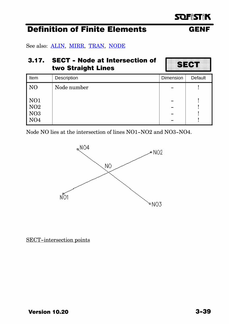
GENFDefinition of Finite Elements
3−39Version 10.20
See also: ALIN, MIRR, TRAN, NODE
3.17. SECT − Node at Intersection of
two Straight Lines
ÄÄÄÄÄÄÄÄÄÄÄÄÄÄÄÄÄÄÄÄÄÄÄÄÄÄÄÄÄÄÄÄ
SECT
Item Description Dimension Default
NO
NO1NO2NO3NO4
Node number −
−−−−
!
!!!!
Node NO lies at the intersection of lines NO1−NO2 and NO3−NO4.
SECT−intersection points

GENFDefinition of Finite Elements
3−41Version 10.20
3.18. Materials
SOFiSTiK supports a large number of different material descriptions. All willbe addressed by a unique material number and should be usable everywherein general. The default for the material type is dependant on the selected de�sign code.
The basic properties are input via the records:
NORM Selection of a design code familyMAT General Materialdefinition (obsolete)MATE General Materialdefinition including strengthCONC Concrete MaterialSTEE Steel and other metallic materialsTIMB Timber/lumberMASO Masonry / BrickworkMLAY Layered composite material for QUAD−Elements
These records are mutually exclusive but may be enhanced by other records:
BMAT Elastic support
NMAT Nonlinear material properties for MAT/MATE(to be used in ASE/TALPA for QUAD and BRIC el�ements)
SSLA uniaxial strain−stress law for materials CONC/STEE/TIMB/BRWO
MEXT Special material properties
Input of material is possible in all parts of the program system. However itis self−evident that not all parameters are used for all types of analysis or sys�tem. Each material has a standard name given by its classification, whichmight be extended by the user. If the user wants to replace the standard com�pletely, he has to start his own text with an equal sign (e.g. ’=my own Text’).
Properties of materials must be distinguished according to whether they areto be kept as close as possible to real values (e.g. for dynamic calculations) orto be used with a safety coefficient for calculating an ultimate load−bearingcapacity. Whereas the safety factors were formerly assigned more−or−less atrandom, sometimes to the load and sometimes to the material, more recentregulations (Eurocode) provide a clearer separation between safety factorsfor the loads and factors for the material. However, since the material safety

GENF Definition of Finite Elements
Version 10.203−42
factors still depend on the nature of the load or the type of design, it will notbe possible to define all safety factors with the material itself.
SOFiSTiK distinguishes therefore:
• Properties and safety factors for the standard Design
• Mean values or calculatoric values and safety factors for serviceabilityand deformation analysis
If some design codes (DIN 18800, DIN 1045−1) apply additional safety−fac�tors to the mean values, this may be defined with the stress−strain relationvia SSLA. The safety factor defined with the material will thus be used onlyfor the full plastic forces in AQUA.
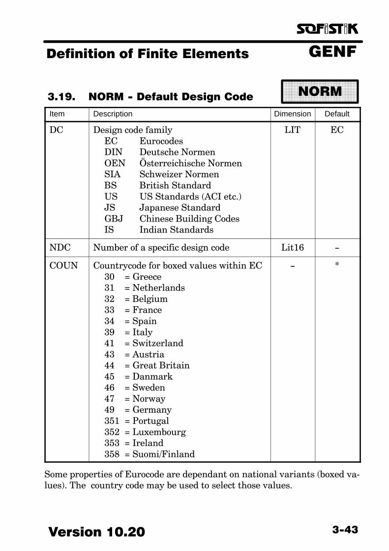
GENFDefinition of Finite Elements
3−43Version 10.20
3.19. NORM − Default Design Code
ÖÖÖÖÖÖÖÖÖÖÖÖÖÖÖÖÖÖÖÖÖÖÖÖÖÖÖÖÖÖÖÖ
NORM
Item Description Dimension Default
DC Design code familyEC EurocodesDIN Deutsche NormenOEN Österreichische NormenSIA Schweizer NormenBS British StandardUS US Standards (ACI etc.)JS Japanese StandardGBJ Chinese Building CodesIS Indian Standards
LIT EC
NDC Number of a specific design code Lit16 −
COUN Countrycode for boxed values within EC30 = Greece31 = Netherlands32 = Belgium33 = France34 = Spain 39 = Italy 41 = Switzerland43 = Austria44 = Great Britain45 = Danmark46 = Sweden 47 = Norway 49 = Germany351 = Portugal352 = Luxembourg353 = Ireland358 = Suomi/Finland
− *
Some properties of Eurocode are dependant on national variants (boxed va�lues). The country code may be used to select those values.

GENF Definition of Finite Elements
Version 10.203−44
3.20. MAT − General Material
Properties
ÖÖÖÖÖÖÖÖÖÖÖÖÖÖÖÖÖÖÖÖÖÖÖÖÖÖÖÖÖÖÖÖÖÖÖÖ
MAT
Item Description Dimension Default
NO
EMUEGKGAMGAMAALFA
Material number
Elastic modulusPoisson’s ratio (between 0 and 0.49)Shear modulusBulk modulusSpecific weightSpecific weight under buoyancyThermal expansion coefficient
−
kN/m2
−kN/m2
kN/m2
kN/m3
kN/m3
−
1
*0.2**
25*
E−5
EYMXYOAL
OAF
SPM
TITL
Anisotropic elastic modulus EyAnisotropic poisson’s ratio m−xyMeridian angle of anisotropyabout the local x−axisDescent angle of anisotropyabout the local x−axisMaterial safety factor
Material name
kN/m2
−deg
deg
−
Lit32
EMUE
0
0
1.0
−
The record MAT can define general materials that can be used for sections orQUAD and BRIC−elements. The material number must be unique for everymaterial.
This record has been superseeded by MATE, supplying input of strength andelasticity constants in MPa. Further comments are available there.
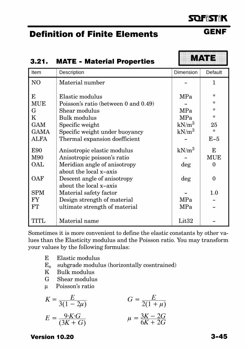
GENFDefinition of Finite Elements
3−45Version 10.20
3.21. MATE − Material Properties
ÖÖÖÖÖÖÖÖÖÖÖÖÖÖÖÖÖÖÖÖÖÖÖÖÖÖÖÖÖÖÖÖ
MATE
Item Description Dimension Default
NO
EMUEGKGAMGAMAALFA
Material number
Elastic modulusPoisson’s ratio (between 0 and 0.49)Shear modulusBulk modulusSpecific weightSpecific weight under buoyancyThermal expansion doefficient
−
MPa−
MPaMPa
kN/m3
kN/m3
−
1
****
25*
E−5
E90M90OAL
OAF
SPMFYFT
TITL
Anisotropic elastic modulusAnisotropic poisson’s ratioMeridian angle of anisotropyabout the local x−axisDescent angle of anisotropyabout the local x−axisMaterial safety factorDesign strength of materialultimate strength of material
Material name
kN/m3
−deg
deg
−MPaMPa
Lit32
EMUE
0
0
1.0−−
−
Sometimes it is more convenient to define the elastic constants by other va�lues than the Elasticity modulus and the Poisson ratio. You may transformyour values by the following formulas:
E Elastic modulusEs subgrade modulus (horizontally cosntrained)K Bulk modulusG Shear modulusµ Poisson’s ratio
K� E3(1� 2�)
G� E2(1��)
E� 9·K·G(3K�G)
�� 3K� 2G6K� 2G
GENF Definition of Finite Elements
Version 10.203−46
Es�E��1���
(1��)(1�2�)
G� 3·K·E9·K�E
G� 3·K·(1� 2�)2·(1��)
If not specified, missing values will be calculated according to these formulas.It is however possibel to define non consistent constants. If no values aregiven, E will default to 30000 MPa and MUE to 0.2.
Orthotropy may be defined via material and thickness of QUAD−Elements.(confer record GRP in GENF and remarks in manuals to ASE, SEPP andTALPA).
The description of a transversal orthotropie according to Lechnitzky has onedirection that has different properties, while the description in the plane per�pendicular to this remains isotropic. This covers most practical problems liketimber and rock. If this special direction is z it holds:
�x� �xE��·
�yE��90· �z
E90
�y��yE��·�x
E��90· �z
E90
�z� �zE90
��90·(�x��y)
E90
Please mark, that the poisson ratio M90 is no longer bound to 0.5 and isstrongly connected to the Elasticity modulus.
For beams the main value of the fibres is the x−axis, perpendicular values yand z will be E90 and M90.
For planar systems (TALPA) the basic values are in the x−z plane. The valueOAF is the angle between the local x−direction and the global x−direction. Youhave to exchange the indices y and z in the above formula.
For shells and plates (ex. plywood) we assume that the fibres are in both x andy direction. The anisotropy effects reduce to different shear moduli for inplane shear and the transverse directions.
For three dimensional continua, the orientation is given by the meridina anddecent angle, known from geology. They describe the deviation of the constant
GENFDefinition of Finite Elements
3−47Version 10.20
height lines to the north direction and the inclination of the layers. They areequivalent to first and third of the Euler angles. The transformation is de�fined by two rotations to be selected by the gravity direction. North is thecyclic permutation of the gravity. (ie. x−axis for GDIR ZZ or NEGZ, y−axisfor GDIR XX or NEGX and z−axis for GDIR YY or NEGY). First the north−axis will be rotated about the vertical axis by the amount of OAF, then therotated x’−y’ plane will be rotated about the x’−axis by the amount of OALagainst the vertical.

GENF Definition of Finite Elements
Version 10.203−48
3.22. MLAY − Layered Material
ÖÖÖÖÖÖÖÖÖÖÖÖÖÖÖÖÖÖÖÖÖÖÖÖÖÖÖÖÖÖÖÖÖÖÖÖ
MLAY
Item Description Dimension Default
NOT0NO0T1NO1...T9NO9TITL
Number of composite materialThickness of first layerMaterial number of first layerThickness of second layerMaterial number of second layer
Thickness of 9th layerMaterial number of 9th layerMaterial Designation
−*−*−
*−
Lit32
1!!!!
−−−
With MLAY you may define for QUAD elements a composite layered materialof up to 10 layers. Each layer may be defined with an positive absolute thick�ness or a negative relative one. The total thickness of the element will be cali�brated to the sum of the thicknesses of the material definition. If some layershave negative thickness only these layers will be adopted. Otherwise a uni�form scaling will take place.
If you have a sandwich element with two outer laminates with a given thick�ness:
MLAY 1 0.02 1 $$ upper laminate −1.00 2 $$ interior laminate 0.02 1 $$ lower laminate
then this data will be applied to match two QUAD elements with a total thick�ness of 0.10 or 0.15 as follows:
MLAY 1 0.02 1 $$ upper laminate 0.06 2 $$ interior laminate if 0.10 total thickness 0.02 1 $$ untere Deckschicht
MLAY 1 0.02 1 $$ upper laminate 0.11 2 $$ interior laminate if 0.15 total thickness 0.02 1 $$ lower laminate
A standard material definition will also be generated with mean values.

GENFDefinition of Finite Elements
3−49Version 10.20
3.23. BMAT − Elastic Support /
Interface
ÖÖÖÖÖÖÖÖÖÖÖÖÖÖÖÖÖÖÖÖÖÖÖÖÖÖÖÖÖÖÖÖ
BMAT
Item Description Dimension Default
NO Material number − 1
CCTCRACYIELMUECOHDILGAMB
Elastic constant normal to surfaceElastic constant tangential to surfaceMaximum tensile stress of interfaceMaximum stress of interfaceFriction coefficient of interfaceCohesion of interfaceDilatancy coefficientEquivalent mass distribution
kN/m3
kN/m3
kN/m2
kN/m2
−kN/m2
−
t/m2
0.0.0.−−−0.0
REF
MREFH
ReferencePESS Plain stress conditionPAIN Plain strain conditionHALF circular disk on halfspaceCIRC circular hole in infinite diskSPHE sperical hole in infinite space
Number of a reference materialReference dimension (thickness/radius)
LIT
−m
−
NO!
The bedding approach works according to the subgrade modulus theory(Winkler, Zimmermann/Pasternak). It facilitates the definition of elastic sup�ports by an engineering trick which, among others, ignores the shear de�formations of the supporting medium. The bedding effect may be attached tobeam or plate elements, but in general it will be used as an independant singleor distributed element. (see SPRI, BOUN, BEAM or QUAD element and themore general description of BORE−Profiles)
The determination of a reasonable value for the foundation modulus oftenpresents considerable difficulty, since this value depends not only on the ma�terial parameters but also on the geometry and the loading. One must alwayskeep this dependance in mind, when assessing the accuracy of the results ofan analysis using this theory.
The subgrade parameters C and CT will be used for bedding of QUAD−El�ements or or the description of support or interface conditions. A QUAD el�
GENF Definition of Finite Elements
Version 10.203−50
ement of a slab foundation will thus have a concrete material and via BMATthe soil properties attached to the same material number.
If subgrade parameters are assigned to the material of a geometric edge(GLN), spring elements will be generated along that edge based on the widthand the distance of the support nodes.
Instead of a direct value you may select a material and a reference dimensionfor some cases with constant pressure [1]:
• Flat layer with horizontal constraints e.g. for elastic support by col�umns and supporting walls (plane stress condition):
Cs� EH� 1
(1��)(1��) Ct� E
H� 1
2(1��)
• Flat layer with horizontal constraints for sttlements of soil strata(plane strain condition):
Cs� EH� (1��)
(1��)(1�2�) Ct� E
H� 1
(1��)
• Equivalent circular disk with radius R on unlimited halfspace:
Cs�ER� 2�(1��)(1��)
• Circular hole in unlimited disk with plane strain conditions
Cs�ER� 1
(1��)(1�2�) Ct�Cs
• Spherical hole in infinite 3D elsatic continua
Cs�ER� 2
(1��) Ct�Cs
Including a dilatancy factor describing the normal strain induced by shear de�formations, we have for the stresses:
��Cs� (un�DIL�ut)��Ct�ut
Nonlinear effects are controlled by CRAC, YIEL, MUE and COH:

GENFDefinition of Finite Elements
3−51Version 10.20
Cracking: Upon reaching the failure load the interface fails inboth the axial and the lateral direction. The failureload is always a tensile stress.
Yield load: Upon reaching the yield stress, the deformation com�ponent of the interface in its direction increases with�out a corresponding increase of the stress.
Friction coefficient:If a friction and/or a cohesion coefficient are input, thelateral shear can not sustain forces greater than:
Friction coefficient * normal stress + Cohesion
If the axial interface has failed (CRAC), the lateral shear acts only if 0.0 hasbeen input for both friction− coefficient and cohesion.
The nonlinear effects can be taken into account only by a nonlinear analysis.The friction is an effect of the lateral interface, while all other effects act uponthe normal stress.
[1] Katz, C., Werner, H. (1982)Implementation of nonlinear boundary conditions in Finite ElementAnalysisComputers & Structures Vol. 15 No. 3 pp. 299−304

GENF Definition of Finite Elements
Version 10.203−52
3.24. NMAT − Non−linear Material
ÖÖÖÖÖÖÖÖÖÖÖÖÖÖÖÖÖÖÖÖÖÖÖÖÖÖÖÖÖÖÖÖÖÖÖÖ
NMAT
Item Description Dimension Default
NOTYPE
Material numberKind of material law
LINE Linear materialMISE Mise / Drucker Prager lawMOHR Mohr Coulomb lawGUDE Gudehus lawROCK Rock materialFAUL Faults in rock materialLADE Lade lawDUNC Duncan−Chang lawHYPO Schad lawSWEL SwellingMEMB Textile membrane
−LIT
1!
P1P2P3P4...P10
1st parameter of material law2nd parameter of material law3rd parameter of material law4th parameter of material law
...10th parameter of material law
****
*
−−−−
−
The types of the implemented material laws and the meaning of their para�meters can be found in the following pages.
In a linear analysis the yield function for the nonlinear material is merelyevaluated and output. This enables an estimation of the nonlinear regionsfor a subsequent nonlinear analysis.
If TYPE LINE is given, the material remains linear.
3.24.1. Invariants of the stress tensorFor the present chapter, as long as not specified differently, the following con�ventions hold:
I1� �� �x��y��z
Deviatoric stress tensor:

GENFDefinition of Finite Elements
3−53Version 10.20
sx� �� �x�I1
3
sy� �� �y�I1
3
sz� �� �z�I1
3
J2� �� 12
(sx2� sy
2� sz2)� �xy
2� �yz2� �xz
2
J3� �� sxsysz� 2�xy�yz�xz� sx�yz2� sy�xz
2� sz�xy2
�� �� 13
sin�1�
� 3 3� J3
2J2
32
��
; ��
6� ���
6
3.24.2. Material Law MISEElastoplastic material after MISE or DRUCKER−PRAGER with associatedflow rule.
f� �� p2 � I1� J2� � p1
3�� 0
Application range:
Metals and other materials without friction
Parameters:
P1 = Comparison stress [kN/m2]P2 = Friction parameter [−]P3 = Hardening module [kN/m2]P4 = Tensile strength β−z [kN/m2]P5 = Compressive strength (cap) β−c [kN/m2]
Several substitutes for P1 and P2 can be used for the calculation of commonparameters in soil mechanics. Commonly used e.g. is the compression cone:
P1�6ccos�
3� sin� P2�
2sin�
3� (3� sin�)
The values for the internal cone are better suited for plane strain conditions:

GENF Definition of Finite Elements
Version 10.203−54
P1�6ccos�
3� sin� P2�
2sin�
3� (3� sin�)
By specification of parameter P5 the model can optionally be extended by aspherical cap (in principal stress space) that limits the volumetric compres�sive stress to a maximum value. This can be meaningful in particular formainly hydrostatic straining. The cap is defined by:
f� �� �12 � �2
2 � �32� � P5
2 � P52 � P5
2� � 0
Reference:
M.A.ChrisfieldNon−linear Finite Element Analysis of Solids and Structures. Vol. I.Essentials. Chapter 14. Wiley & Sons (1991)
M.A.ChrisfieldNon−linear Finite Element Analysis of Solids and Structures. Ad�vanced Topics. Vol. II. Chapter 6. Wiley & Sons (1997)
3.24.3. Material Law MOHRElastoplastic material with a prismatic yield surface and a non associatedflow rule after MOHR−COULOMB. The model is extended by means of aspherical compression cap and plane tension limits. Formulation of yieldcondition and plastic potential using stress invariants:
f� �� 13I1 sin�� J2
� (cos�� sin� sin�
3�)� ccos�� 0
g� �� 13I1 sin�� J2
� (cos�� sin� sin�3�
)
with:
Application range: soils with friction and cohesion
Parameters: Default values:
P1 = Friction angle ϕ [degrees] (0.)P2 = Cohesion c [kN/m2] (0.)P3 = Tensile strength β−z [kN/m2] (0.)

GENFDefinition of Finite Elements
3−55Version 10.20
P4 = Dilatation angle ν [degrees] (0.)P5 = Compressive strength (cap) β−c [kN/m2] (−)P6 = plastic ultimate strain εu [o/oo] (0.)P7 = ultimate friction angle ϕu [grad] (P1)P8 = ultimate cohesion cu [kN/m2] (P2)
Special comments:
The following expressions are better suited for checking the yield criterion:
f = σI � m ⋅ σIII � b ≤ 0
m� 1� sin�1� sin�
b� 2ccos�1� sin�
By specification of parameter P5 the model can optionally be extended by aspherical cap (in principal stress space) that limits the volumetric compres�sive stress to a maximum value. This can be meaningful in particular formainly hydrostatic straining. The cap is defined by:
f� �� �12 � �2
2 � �32� � P5
2 � P52 � P5
2� � 0
Reference:
M.A.ChrisfieldNon−linear Finite Element Analysis of Solids and Structures. Ad�vanced Topics. Vol. II. Chapter 14. Wiley & Sons (1997)
O.C.Zienkiewicz,G.N.Pande Some Useful Forms of Isotropic Yield Surfaces for Soil and RockMechanics. Chapter 5 in Finite Elements in Geomechanics(G.Gudehus ed.) Wiley & Sons (1977)
3.24.4. Material Law GUDEElastoplastic material in its extended form after Gudehus with non asso�ciated flow rule.
f = q2 − c7 p2 + c6 p − c5 < 0
g = q2 − c9 p2 + c8 p
with:
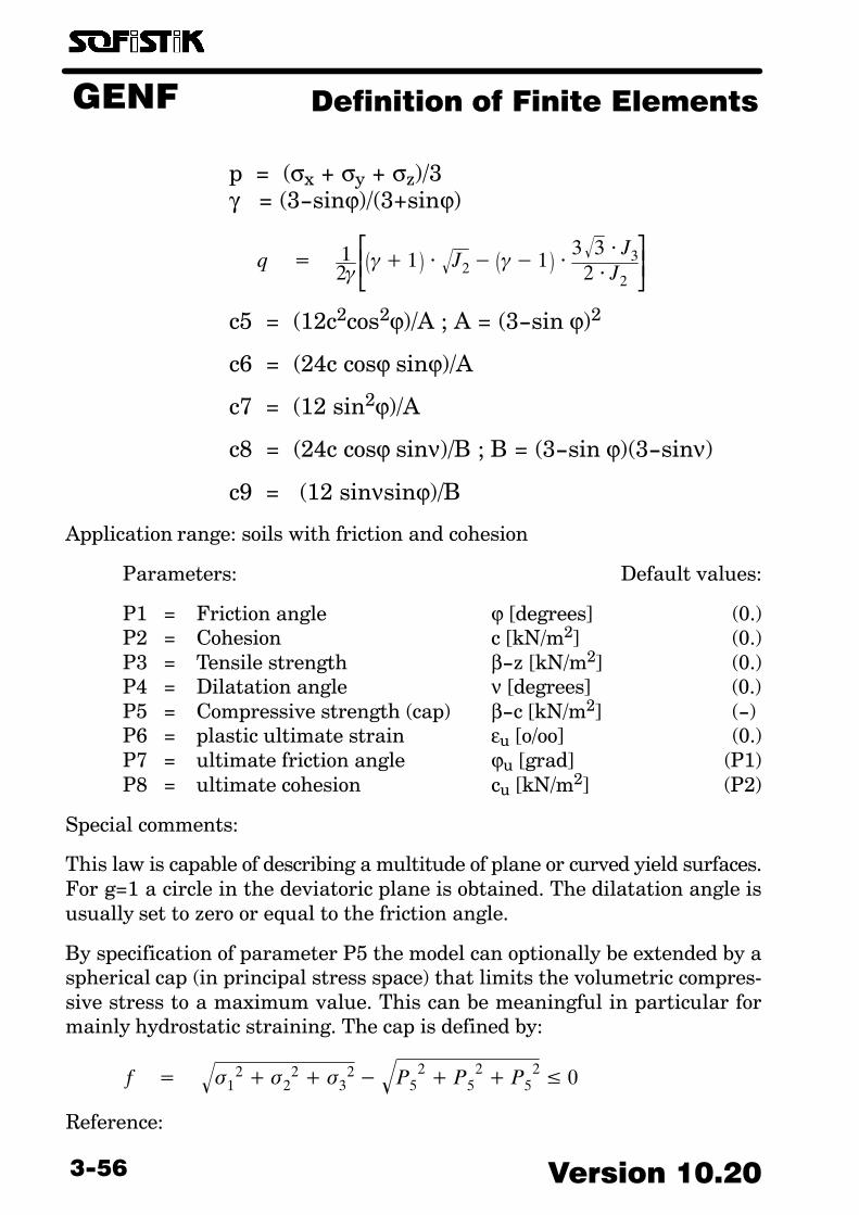
GENF Definition of Finite Elements
Version 10.203−56
p = (σx + σy + σz)/3 γ = (3−sinϕ)/(3+sinϕ)
q� �� 12���1� � J2
� ���1� �3 3� � J3
2� J2��
c5 = (12c2cos2ϕ)/A ; A = (3−sin ϕ)2
c6 = (24c cosϕ sinϕ)/A
c7 = (12 sin2ϕ)/A
c8 = (24c cosϕ sinν)/B ; B = (3−sin ϕ)(3−sinν)
c9 = (12 sinνsinϕ)/B
Application range: soils with friction and cohesion
Parameters: Default values:
P1 = Friction angle ϕ [degrees] (0.)P2 = Cohesion c [kN/m2] (0.)P3 = Tensile strength β−z [kN/m2] (0.)P4 = Dilatation angle ν [degrees] (0.)P5 = Compressive strength (cap) β−c [kN/m2] (−) P6 = plastic ultimate strain εu [o/oo] (0.)P7 = ultimate friction angle ϕu [grad] (P1)P8 = ultimate cohesion cu [kN/m2] (P2)
Special comments:
This law is capable of describing a multitude of plane or curved yield surfaces.For g=1 a circle in the deviatoric plane is obtained. The dilatation angle isusually set to zero or equal to the friction angle.
By specification of parameter P5 the model can optionally be extended by aspherical cap (in principal stress space) that limits the volumetric compres�sive stress to a maximum value. This can be meaningful in particular formainly hydrostatic straining. The cap is defined by:
f� �� �12 � �2
2 � �32� � P5
2 � P52 � P5
2� � 0
Reference:
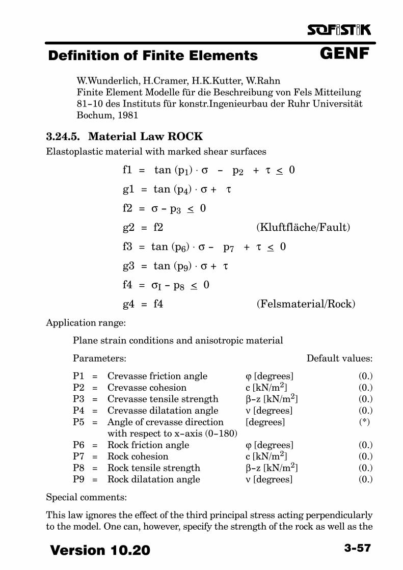
GENFDefinition of Finite Elements
3−57Version 10.20
W.Wunderlich, H.Cramer, H.K.Kutter, W.Rahn Finite Element Modelle für die Beschreibung von Fels Mitteilung81−10 des Instituts für konstr.Ingenieurbau der Ruhr UniversitätBochum, 1981
3.24.5. Material Law ROCKElastoplastic material with marked shear surfaces
f1 = tan (p1) ⋅ σ − p2 + τ < 0
g1 = tan (p4) ⋅ σ + τ
f2 = σ − p3 < 0
g2 = f2 (Kluftfläche/Fault)
f3 = tan (p6) ⋅ σ − p7 + τ < 0
g3 = tan (p9) ⋅ σ + τ
f4 = σI − p8 < 0
g4 = f4 (Felsmaterial/Rock)
Application range:
Plane strain conditions and anisotropic material
Parameters: Default values:
P1 = Crevasse friction angle ϕ [degrees] (0.)P2 = Crevasse cohesion c [kN/m2] (0.)P3 = Crevasse tensile strength β−z [kN/m2] (0.)P4 = Crevasse dilatation angle ν [degrees] (0.)P5 = Angle of crevasse direction [degrees] (*)
with respect to x−axis (0−180)P6 = Rock friction angle ϕ [degrees] (0.)P7 = Rock cohesion c [kN/m2] (0.)P8 = Rock tensile strength β−z [kN/m2] (0.)P9 = Rock dilatation angle ν [degrees] (0.)
Special comments:
This law ignores the effect of the third principal stress acting perpendicularlyto the model. One can, however, specify the strength of the rock as well as the
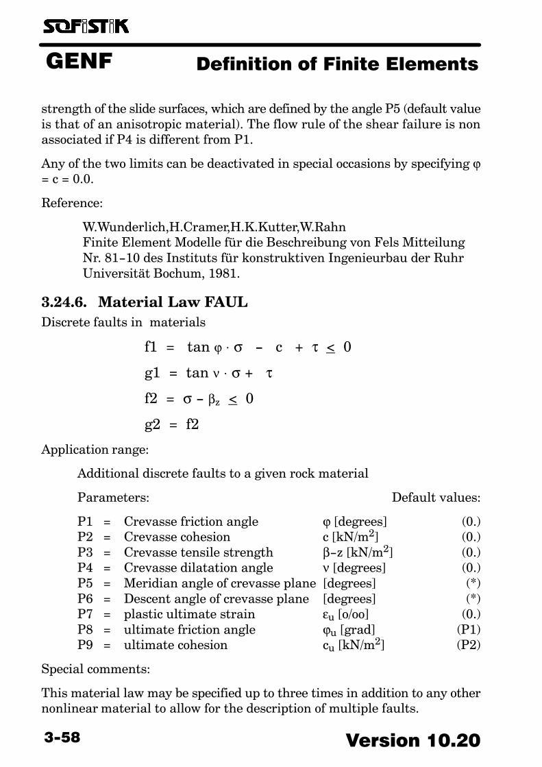
GENF Definition of Finite Elements
Version 10.203−58
strength of the slide surfaces, which are defined by the angle P5 (default valueis that of an anisotropic material). The flow rule of the shear failure is nonassociated if P4 is different from P1.
Any of the two limits can be deactivated in special occasions by specifying ϕ= c = 0.0.
Reference:
W.Wunderlich,H.Cramer,H.K.Kutter,W.Rahn Finite Element Modelle für die Beschreibung von Fels MitteilungNr. 81−10 des Instituts für konstruktiven Ingenieurbau der RuhrUniversität Bochum, 1981.
3.24.6. Material Law FAULDiscrete faults in materials
f1 = tan ϕ ⋅ σ − c + τ < 0
g1 = tan ν ⋅ σ + τ
f2 = σ − βz < 0
g2 = f2
Application range:
Additional discrete faults to a given rock material
Parameters: Default values:
P1 = Crevasse friction angle ϕ [degrees] (0.)P2 = Crevasse cohesion c [kN/m2] (0.)P3 = Crevasse tensile strength β−z [kN/m2] (0.)P4 = Crevasse dilatation angle ν [degrees] (0.)P5 = Meridian angle of crevasse plane [degrees] (*)P6 = Descent angle of crevasse plane [degrees] (*)P7 = plastic ultimate strain εu [o/oo] (0.)P8 = ultimate friction angle ϕu [grad] (P1)P9 = ultimate cohesion cu [kN/m2] (P2)
Special comments:
This material law may be specified up to three times in addition to any othernonlinear material to allow for the description of multiple faults.
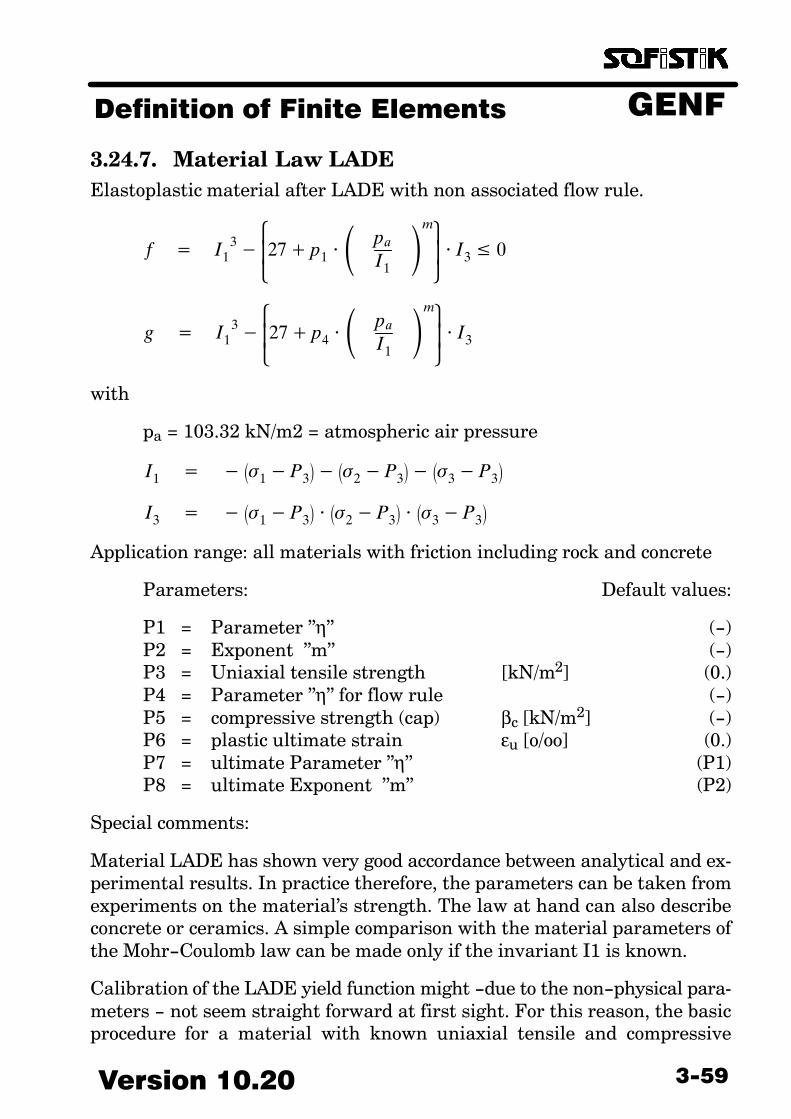
GENFDefinition of Finite Elements
3−59Version 10.20
3.24.7. Material Law LADEElastoplastic material after LADE with non associated flow rule.
f� �� I13��
�
�27� p1���
paI1
��m���� I3 � 0
g� �� I13��
�
�27� p4���
paI1
��m���� I3
with
pa = 103.32 kN/m2 = atmospheric air pressure
I1� �����1�P3�� ��2 �P3
�� ��3�P3�
I3� �����1�P3� � ��2 �P3
� � ��3�P3�
Application range: all materials with friction including rock and concrete
Parameters: Default values:
P1 = Parameter "η" (−)P2 = Exponent "m" (−)P3 = Uniaxial tensile strength [kN/m2] (0.)P4 = Parameter "η" for flow rule (−)P5 = compressive strength (cap) βc [kN/m2] (−)P6 = plastic ultimate strain εu [o/oo] (0.)P7 = ultimate Parameter "η" (P1)P8 = ultimate Exponent "m" (P2)
Special comments:
Material LADE has shown very good accordance between analytical and ex�perimental results. In practice therefore, the parameters can be taken fromexperiments on the material’s strength. The law at hand can also describeconcrete or ceramics. A simple comparison with the material parameters ofthe Mohr−Coulomb law can be made only if the invariant I1 is known.
Calibration of the LADE yield function might −due to the non−physical para�meters − not seem straight forward at first sight. For this reason, the basicprocedure for a material with known uniaxial tensile and compressive
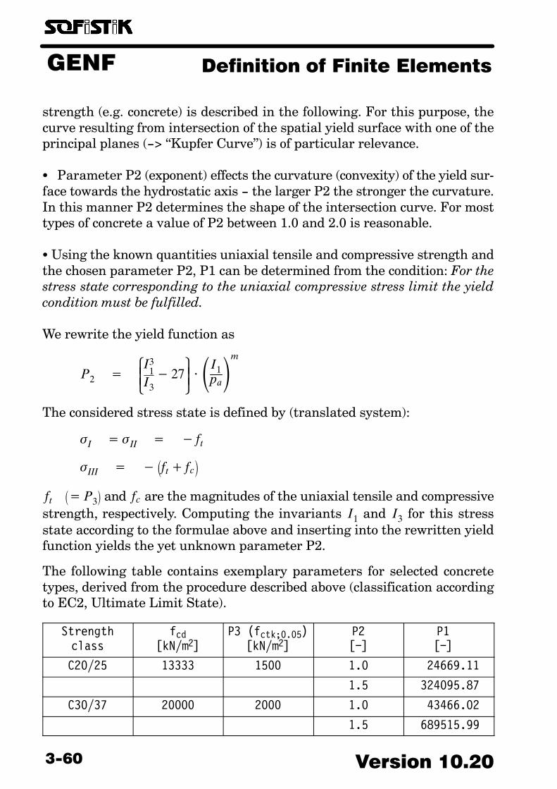
GENF Definition of Finite Elements
Version 10.203−60
strength (e.g. concrete) is described in the following. For this purpose, thecurve resulting from intersection of the spatial yield surface with one of theprincipal planes (−> �Kupfer Curve") is of particular relevance.
� Parameter P2 (exponent) effects the curvature (convexity) of the yield sur�face towards the hydrostatic axis − the larger P2 the stronger the curvature.In this manner P2 determines the shape of the intersection curve. For mosttypes of concrete a value of P2 between 1.0 and 2.0 is reasonable.
� Using the known quantities uniaxial tensile and compressive strength andthe chosen parameter P2, P1 can be determined from the condition: For thestress state corresponding to the uniaxial compressive stress limit the yieldcondition must be fulfilled.
We rewrite the yield function as
P2� �����I3
1
I3
�27�����I1
pa�m
The considered stress state is defined by (translated system):
�I� � �II��� � ft
�III� ����ft� fc�
ft��� P3� and fc are the magnitudes of the uniaxial tensile and compressive
strength, respectively. Computing the invariants I1 and I3 for this stressstate according to the formulae above and inserting into the rewritten yieldfunction yields the yet unknown parameter P2.
The following table contains exemplary parameters for selected concretetypes, derived from the procedure described above (classification accordingto EC2, Ultimate Limit State).
Strengthclass
fcd[kN/m2]
P3 (fctk;0.05)[kN/m2]
P2[−]
P1[−]
C20/25 13333 1500 1.0 24669.11
1.5 324095.87
C30/37 20000 2000 1.0 43466.02
1.5 689515.99

GENFDefinition of Finite Elements
3−61Version 10.20
C40/50 26667 2500 1.0 63426.77
1.5 1153410.57
C50/60 33333 2900 1.0 88162.15
1.5 1778218.62
By specification of parameter P5 the model can optionally be extended by aspherical cap (in principal stress space) that limits the volumetric compres�sive stress to a maximum value. This can be meaningful in particular formainly hydrostatic straining. The cap is defined by:
f� �� �12 � �2
2 � �32� � P5
2 � P52 � P5
2� � 0
Reference:
P.V.LadeFailure Criterion for Frictional Materials in Mechanics ofEngineering Materials, Chap 20 (C.s.Desai,R.H.Gallagher ed.)Wiley & Sons (1984)
3.24.8. Material Law DUNCHypoelastic material based on Duncan−Chang.
Loading:
Et� ���
1 �
p7 � �1 � sin�p1�� � ��I� �III
�
2 � p2 � cos�p1� � 2 � �I � sin�p1
���
2
��p4��
max��p3 � �I
�, 0�pa �
�
p6
Unloading and reloading:
Et� �� p5��
max��p3 � �I�, 0�
pa ��
p6
pa = 103.32 kN/m2 = atmospheric air pressure
Application range:Deformation analyses with little plastification and with stress paths not verydifferent from a triaxial test.

GENF Definition of Finite Elements
Version 10.203−62
Parameters: Default values:
P1 = Friction angle ϕ [degrees] (0.)P2 = Cohesion c [kN/m2] (0.)P3 = Tensile strength β−z [kN/m2] (0.)P4 = Reference elastic modulus [kN/m2] (−)
during loadingP5 = Reference elastic modulus [kN/m2] (−)
during unloadingP6 = Exponent (� 0) [−] (−)P7 = Calibration factor (� 0) [−] (−)
Special comments:
The model distinguishes between primary loading, unloading and reloading− different moduli for loading and un−/reloading can be specified.
Loading is defined as an increase of the stress level S:
S� �������
�1� sin�p1�� � ��I��III�
2� p2� cos�p1��2� �I� sin�p1
������
The initial state should be calculated linearly − doing so, parameters definingthe loading history are initialized and the resulting stress state is interpretedas �loading".
In case of unloading, after having passed a deviatoric stress minimum, a pri�mary loading branch is traced again −> simulation of cyclic loading behavioris possible.
The original law according to DUNCAN/CHANG has been modified in orderto allow for a better simulation of the plastic flow in soil materials. Poisson’sratio is not kept constant but is defined as a function of the tangential modu�lus of elasticity and the bulk modulus. The bulk modulus is kept constant inthis case.
By P6=P7=0 one can define a law with each a constant elastic modulus forloading and unloading.
In order to avoid numerical difficulties, the elastic modulus in the MAT re�cord should not be chosen smaller than the initial elastic modulus.
Anisotropic materials are not possible with this model.

GENFDefinition of Finite Elements
3−63Version 10.20
Reference:
J.M.Duncan, C.Y.ChangNonlinear Analysis of Stress and Strains in SoilsJ.Soil.Mech.Found.Div. ASCE Vol 96 SM 5 (1970) ,1629−1653
C.S.Desai, J.T.ChristianNumerical Methods in Geotechnical Engineering, 81−88 McGraw−Hill Book Company
3.24.9. Material Law HYPOHypoelastic material after Schad.
Bulk and shear moduli during loading:
K = p1 − p7 ⋅ p − p8 ⋅ qmax
G = p2 − p5 ⋅ (σI+σIII) − p6 ⋅ q
Bulk and shear moduli during unloading:
K = p3
G = p4
where:
p = (σx + σy + σz)/3
q = σI − σIII
Application range: isotropic materials
Parameters: Default values:
P1 = Initial bulk modulus [kN/m2] (−)P2 = Initial shear modulus [kN/m2] (−)P3 = Bulk modulus for unloading [kN/m2] (−)P4 = Shear modulus for unloading [kN/m2] (−)P5 = Parameter [−] (−)P6 = Parameter [−] (−)P7 = Parameter [−] (−)P8 = Parameter [−] (−)P9 = Tensile strength [kN/m2] (0)

GENF Definition of Finite Elements
Version 10.203−64
Special comments:
This law must have a vanishing shear modulus at failure by Mohr−Coulomb,thus the following expressions are obtained:
p2 = p6 ⋅ 2 ⋅ c ⋅ cos ϕ
p5 = p6 ⋅ sin ϕ
Anisotropic Material constants are not possible with this model.
Reference:
H.SchadNichtlineare Stoffgleichungen für Böden und ihre Verwendung beider numerischen Analyse von Grundbauaufgaben. MitteilungenHeft 10 des Baugrund−Instituts Stuttgart (1979)
3.24.10. Material law SWELAdditional Parameters for swelling of materials
Application range: Selling of soils in case of unloading
Relationship between stress and final state swelling strains:
�qi�
� ��� p1���
���
�
�
�
0�������� i� �0i
log� �i�0i������0i� �i��p2
log��c�0i�����p2 � � i
i� �� 1..3
�i = principal normal stresses�0i = equilibrium state of stress wrt swelling (initial condition),
transformed to the direction of principal normal stresses �i
Parameters: Default values:
P1 = modulus of swelling [−] (0.0033)P2 = magnitude of the smallest compressive stress below which
no more increase of swelling occurs [kN/m2] (10.0)
GENFDefinition of Finite Elements
3−65Version 10.20
Special comments:
Swelling of soils is a complex phemomenon that is influenced by various fac�tors. There are two swelling mechanisms of practical importance that can bedistingushed − for which the presence of (pore−) water is a common prerequi�site. The first mechanism is termed as the �osmotic swelling" of clay minerals,which basically is initiated by unloading of clayey sedimentary rock. The sec�ond mechanism takes place in sulfate−laden rock with anhydrite content. Inthis case the swelling effects are due to the chemical transformation of anhy�drite to gypsum− which goes along with a large increase in volume (61%).
For both described mechanisms a principal dependency between the swell�ing−caused increase in volume and the state of stress was observed both inlaboratory and in in−situ experiments. The formula employed here, repre�sents a generalization of the 1−dimensional stress−strain relationship, whichHUDER and AMBERG derived from oedometer tests.
The equilibrium state wrt swelling �0 is defined by means of the GRP−record.Doing so, we use the option PLQ in order to reference a (previously calculated)load case as �primary state for swelling". This state is in equilibrium wrtswelling (normally in−situ soil prior to construction work). In the course ofconstruction work occuring unloading related to this primary state causesswelling strains according to the formula above.
The SWEL record is specified in addition to a linear elastic or elastoplasticbasic material.
Anisotropy is not possible with this model.
Reference:
P.Wittke−Gattermann Verfahren zur Berechnung von Tunnels in quellfähigem Gebirgeund Kalibrierung an einem Versuchsbauwerk. Dissertation RWTH−Aachen, Verlag Glückauf 1998
W.Wittke Grundlagen für die Bemessung und Ausführung von Tunnels inquellendem Gebirge und ihre Anwendung beim Bau derWendeschleife der S−Bahn Stuttgart. Veröffentlichungen des Institutes für Grundbau, Bodenmechanik,Felsmechanik und Verkehrswasserbau der RWTH−Aachen 1978
GENF Definition of Finite Elements
Version 10.203−66
W.Wittke, P.RisslerBemessung der Auskleidung von Hohlräumen in quellendemGebirge nach der Finite Element Methode. Veröffentlichungen des Institutes für Grundbau, Bodenmechanik,Felsmechanik und Verkehrswasserbau der RWTH−Aachen 1976,Heft 2, 7−46
Nichtlineare Stoffgleichungen für Böden und ihre Verwendung beider numerischen Analyse von Grundbauaufgaben. MitteilungenHeft 10 des Baugrund−Instituts Stuttgart (1979)
3.24.11. Material law MEMBParameters for textile membranes
P1 Factor for Stress change(only in special cases, cnf. ASE GRP FACS)
P2 Factor for compression stiffness0.0 no compressive stress possible1.0 full compressive stress possible0.1 intermediate values for scaling the elasticity modulus

GENFDefinition of Finite Elements
3−67Version 10.20
3.25. MEXT − Extra
Materialconstants
ÖÖÖÖÖÖÖÖÖÖÖÖÖÖÖÖÖÖÖÖÖÖÖÖÖÖÖÖÖÖÖÖ
MEXT
Item Description Dimension Default
NOTYPEVALVAL1VAL2VAL3VAL4VAL5
Number of materialType of constantValue of material constantFirst additional material valueSecond additional material valueThird additional material value4th additional material value5th additional material value
−LIT
******
1!−−−−−−
With MEXT you may define special material values for any type of material.The definition of TYPE selects one of the following possibilities:
With KR VAL defines the equivalent roughness according to Table 10.8.1 ofEC 1 part 2−4, needed especially for wind loads on circular sections:
Surface Roughnessk [mm]
Surface Roughnessk [mm]
glas 0.0015 galvanised steel 0.2
polished metall 0.002 spinning concrete 0.2
smooth painting 0.006 cast in situ con�crete
1.0
spray painting 0.02 rust 2.0
blasted steel 0.05 masonry 3.0
cast iron 0.2
Hint: In table 4 of DIN 1055 part 4 slightly larger values are defined .
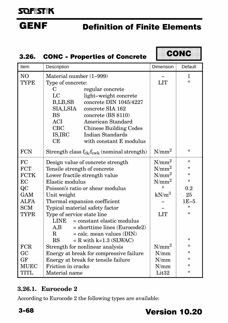
GENF Definition of Finite Elements
Version 10.203−68
3.26. CONC − Properties of Concrete
ÖÖÖÖÖÖÖÖÖÖÖÖÖÖÖÖÖÖÖÖÖÖÖÖÖÖÖÖÖÖÖÖÖÖÖÖ
CONC
Item Description Dimension Default
NOTYPE
Material number (1−999)Type of concrete:
C regular concreteLC light−weight concreteB,LB,SB concrete DIN 1045/4227SIA,LSIA concrete SIA 162BS concrete (BS 8110)ACI American StandardCBC Chinese Building CodesIS,IRC Indian StandardsCE with constant E modulus
−LIT
1*
FCN Strength class fck/fcwk (nominal strength) N/mm2 *
FCFCTFCTKECQCGAMALFASCMTYPR
FCRGCGFMUECTITL
Design value of concrete strengthTensile strength of concreteLower fractile strength valueElastic modulusPoisson’s ratio or shear modulusUnit weightThermal expansion coefficientTypical material safety factorType of service state line
LINE = constant elastic modulus A,B = shorttime lines (Eurocode2)R = calc. mean values (DIN)RS = R with k=1.3 (SLWAC)
Strength for nonlinear analysisEnergy at break for compressive failureEnergy at break for tensile failureFriction in cracksMaterial name
N/mm2
N/mm2
N/mm2
N/mm2
*kN/m3
−−
LIT
N/mm2
N/mmN/mmN/mmLit32
****
0.225
1E−5**
******
3.26.1. Eurocode 2
According to Eurocode 2 the following types are available:
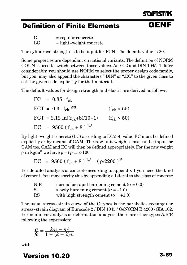
GENFDefinition of Finite Elements
3−69Version 10.20
C = regular concreteLC = light−weight concrete
The cylindrical strength is to be input for FCN. The default value is 20.
Some properties are dependant on national variants. The definition of NORMCOUN is used to switch between those values. As EC2 and DIN 1045−1 differconsiderably, you should use NORM to select the proper design code family,but you may also append the characters �:DIN" or �.EC" to the given class toset the given code explicitly for that material.
The default values for design strength and elastic are derived as follows:
FC = 0.85 ⋅ fck
FCT = 0.3 ⋅ fck 2/3 (fck < 55)
FCT = 2.12 ln((fck+8)/10+1) (fck > 50)
EC = 9500 ( fck + 8 ) 1/3
By light−weight concrete (LC) according to EC2−4, value EC must be definedexplicitly or by means of GAM. The raw unit weight class can be input forGAM too, GAM and EC will then be defined appropriately. For the raw weightρ in kg/m3 we have ρ = (γ−1.5)⋅100
EC = 9500 ( fck + 8 ) 1/3 ⋅ ( ρ/2200 ) 2
For detailed analysis of concrete according to appendix 1 you need the kindof cement. You may specify this by appending a Literal to the class of concrete
N,R normal or rapid hardening cement (α = 0.0)S slowly hardening cement (α = −1.0)RS with high strength cement (α = +1.0)
The usual stress−strain curve of the C types is the parabolic− rectangularstress−strain diagram of Eurocode 2 / DIN 1045 / OeNORM B 4200 / SIA 162.For nonlinear analysis or deformation analysis, there are other types A/B/Rfollowing the expression:
�fc� k·n� n2
1� (k�2)·n
with

GENF Definition of Finite Elements
Version 10.203−70
n = ε / εc1
k = (1.1⋅EC) ⋅ εc1/fc
For fc we have for the curves A and B the value fck+8, for R or RS the value0.85αfck according to DIN 1045−1. The maximum strain is limited accordingto the strength. The B line does not possess a falling branch, and it is thuseventually more stable numerically.
The safety factors SCM are preset to 1.5. In AQB, however, they must be se�lected explicitly, because they are dependent on the loading combinations.For concrete with high strength the factor will be increased by γ’, which willalso be incorporated in the strain−stress laws, to allow a global safety factorto be used for the design.
For nonlinear analysis with a constant safety factor according to DIN 1045−1the strength of the concrete will be reduced, while those of the steel will beraised. This servicability work law is selected with the literal R at positionTYPR. As DIN 1045−1 distinguishes between normal and light sand, thelatter may be adressed with the literal RS.
3.26.2. DIN 1045 old / DIN 4227 / DIN 18806:
The new DIN 1045 will be addressed by the national variant of Eurocode EC2. The old DIN can be addressed with the old literals.
B = regular concrete (DIN)LB = light−weight concrete (DIN)SB = pre−stressed concrete (DIN)
The default FCN is 25 for B and LB, and 45 for SB. FCT is defined by:
FCT = 0.25 ⋅ FCN 2/3
Defaults in accordance with old DIN 1045 / DIN 4227:
FCN 10 15 25 35 45 55
FCDIN 1045 (B)DIN 4227 (SB)
EC
7–
22000
10.5–
26000
17.515.0
30000
2321
34000
2727
37000
3033
39000
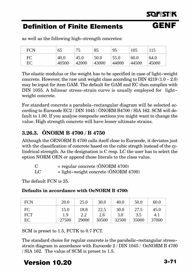
GENFDefinition of Finite Elements
3−71Version 10.20
as well as the following high−strength concretes:
FCN 65 75 85 95 105 115
FCEC
40.040500
45.042000
50.043000
55.044000
60.044500
64.045000
The elastic modulus or the weight has to be specified in case of light−weightconcrete. However, the raw unit weight class according to DIN 4219 (1.0 − 2.0)may be input for item GAM. The default for GAM and EC then complies withDIN 1055. A bilinear stress−strain curve is usually employed for light−weight concrete.
For standard concrete a parabola−rectangular diagram will be selected ac�cording to Eurocode EC2 / DIN 1045 / ÖNORM B4700 / SIA 162. SCM will de�fault to 1.00. If you analyse composite sections you might want to change thevalue. High strength concrete will have lesser ultimate strains.
3.26.3. ÖNORM B 4700 / B 4750Although the OENORM B 4700 calls itself close to Eurocode, it deviates justwith the classification of concrete based on the cubic stregth instead of the cy�lindrical strength. As the designation is C resp. LC the user has to select theoption NORM OEN or append those literals to the class value.
C = regular concrete (ÖNORM 4700)LC = light−weight concrete (ÖNORM 4700)
The default FCN is 25.
Defaults in accordance with OeNORM B 4700:
FCN 20.0 25.0 30.0 40.0 50.0 60.0
FCFCTEC
15.01.9
27500
18.82.2
29000
22.52.6
30500
30.03.0
32500
27.53.5
35000
45.04.1
37000
SCM is preset to 1.5, FCTK to 0.7⋅FCT.
The standard choice for regular concrete is the parabolic−rectangular stress−strain diagram in accordance with Eurocode 2 / DIN 1045 / OeNORM B 4700/ SIA 162. The value of SCM is preset to 1.5.
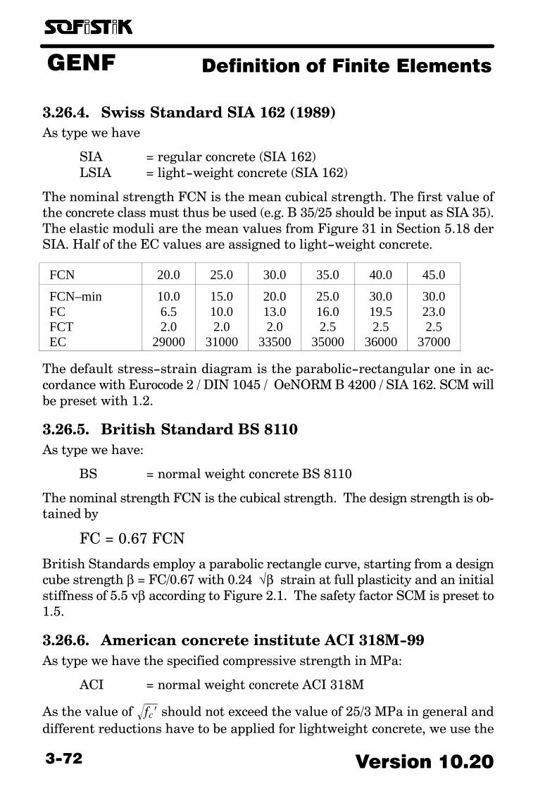
GENF Definition of Finite Elements
Version 10.203−72
3.26.4. Swiss Standard SIA 162 (1989)As type we have
SIA = regular concrete (SIA 162)LSIA = light−weight concrete (SIA 162)
The nominal strength FCN is the mean cubical strength. The first value ofthe concrete class must thus be used (e.g. B 35/25 should be input as SIA 35).The elastic moduli are the mean values from Figure 31 in Section 5.18 derSIA. Half of the EC values are assigned to light−weight concrete.
FCN 20.0 25.0 30.0 35.0 40.0 45.0
FCN–minFCFCTEC
10.06.52.0
29000
15.010.02.0
31000
20.013.02.0
33500
25.016.02.5
35000
30.019.52.5
36000
30.023.02.5
37000
The default stress−strain diagram is the parabolic−rectangular one in ac�cordance with Eurocode 2 / DIN 1045 / OeNORM B 4200 / SIA 162. SCM willbe preset with 1.2.
3.26.5. British Standard BS 8110As type we have:
BS = normal weight concrete BS 8110
The nominal strength FCN is the cubical strength. The design strength is ob�tained by
FC = 0.67 FCN
British Standards employ a parabolic rectangle curve, starting from a designcube strength β = FC/0.67 with 0.24 √β strain at full plasticity and an initialstiffness of 5.5 vβ according to Figure 2.1. The safety factor SCM is preset to1.5.
3.26.6. American concrete institute ACI 318M−99As type we have the specified compressive strength in MPa:
ACI = normal weight concrete ACI 318M
As the value of fc�� should not exceed the value of 25/3 MPa in general anddifferent reductions have to be applied for lightweight concrete, we use the

GENFDefinition of Finite Elements
3−73Version 10.20
tensile stress to define the value of fc�� . The modulus of rupture fr is theupper fractile value of the tension strength. ACI 9.5.2.3 defines:
fr� 0.75 * fc�� � 0.75 * 25�3
or for lightweight concrete:
fr� 0.70 * min( fc�� , 1.8 * fct�m)
fr� 0.70 * 0.75 * fc��
The ratio of the fractiles is thus 1.26. The mean value fct−m will be preset to0.5 * fc�� . All other values will be derived from this value by a factor. If neededthe lower fractile may be given, which will then set the upper value. But thisvalue is only used for those cases where explicitly the value fr is used withina formula.
3.26.7. Chinese StandardsAs type we have:
SGBJ = Standard TB 10002.3−99 (Railway Bridge)
The nominal strength FCN (15 to 60) and the the design strength are takenfrom table 3.1.3. Youngs modulus is derived from 3.1.4.
3.26.8. Indian Standards IS 456 / IRC 21As type we have:
IS = Indian Standards IS 456 (10 bis 80)IRC = Indian Roads Congress IRC 21 (15 bis 60)
The nominal strength FCN is the cubical strength. The design strength is ob�tained by
FC = 0.67 FCN
Indish Standards employ either allowed stresses (IRC resp. Annex B of IS456) or a parabolic rectangular curve with 2 and 2.5 o/oo strain. The allowedstresses will be converted to a serviceability stress strain law. The elasticitymodulus is preset according to IS to 5000 * fck� , for IRC according to table 9.
The tensile strength is preset to 0.7 * fck� . The safety factor SCM is preset to1.5.

GENF Definition of Finite Elements
Version 10.203−74
3.26.9. Linear Elastic ConceteA linear elastic material without tensile stresses is specified for CE. This canbe used for servicability analysis, older design codes or stresses of founda�tions.

GENFDefinition of Finite Elements
3−75Version 10.20
3.27. STEE − Properties of Metals
ÖÖÖÖÖÖÖÖÖÖÖÖÖÖÖÖÖÖÖÖÖÖÖÖÖÖÖÖÖÖÖÖ
STEE
Item Description Dimension Default
NRTYPE
CLAS
Material number (1−999)Type of the material
S / PS reinforc./prestress. steelBST/PST Reinf./prestr. steel DINFE / S / ST Structural steel EC/DINGU Cast ironAL,AC,AW Aluminium alloymore types see comments
Steel class or quality
−LIT
*
1*
*
FYFTFPESQSGAMALFA
SCM
Yield strength (f0.02)Tensile strengthElastic limit (f0.01)Elastic modulusPoisson’s ratio or shear modulusUnit weightThermal expansion coefficient
Default for AL:Typical material safety factor
N/mm2
N/mm2
N/mm2
N/mm2
*kN/m3
−
****
0.3*
1.2E−52.38E−5
*
EPSYEPSTREL1REL2RK1FDYNTITL
Permanent strain at yield strengthUltimate strainCoefficient of relaxation (0.70 βΖ)Coefficient of relaxation (0.55 βΖ)Bond coefficient by DIN 4227 Table 8.1Bond coefficient per EC 2 / Vol. 400Allowed stress rangeMaterial name
o/ooo/oo%%−−
N/mm2
Lit32
***0
150/2002.0/0.8
**
The steel types S (partial), FE, ST, GU, BS, A and AL, AC, AW can be usedfor cross−sections. All other designations can be used only as reinforcementand prestressing tendons. The safety factors are considered by AQB first, be�cause they depend on the loading combination.
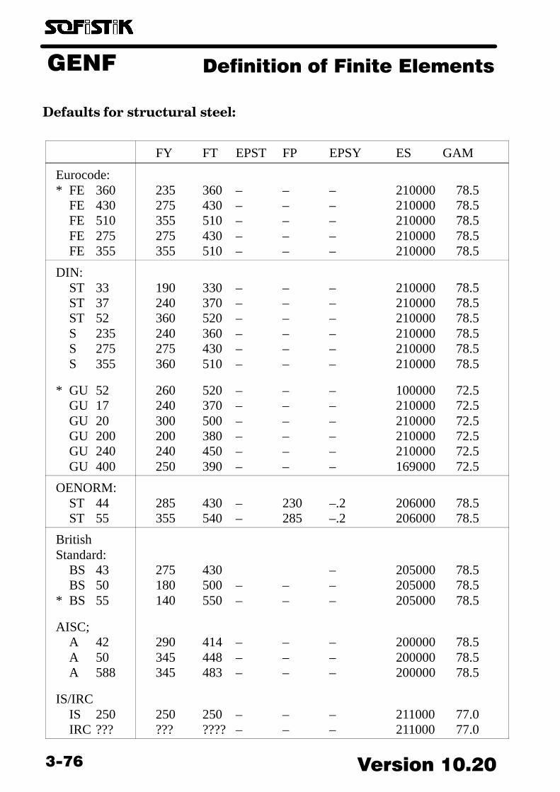
GENF Definition of Finite Elements
Version 10.203−76
Defaults for structural steel:
FY FT EPST FP EPSY ES GAM
Eurocode:* FE 360
FE 430FE 510FE 275FE 355
235 360 – – – 210000 78.5275 430 – – – 210000 78.5355 510 – – – 210000 78.5275 430 – – – 210000 78.5355 510 – – – 210000 78.5
DIN:ST 33ST 37ST 52S 235S 275S 355
* GU 52GU 17GU 20GU 200GU 240GU 400
190 330 – – – 210000 78.5240 370 – – – 210000 78.5360 520 – – – 210000 78.5240 360 – – – 210000 78.5275 430 – – – 210000 78.5360 510 – – – 210000 78.5
260 520 – – – 100000 72.5240 370 – – – 210000 72.5300 500 – – – 210000 72.5200 380 – – – 210000 72.5240 450 – – – 210000 72.5250 390 – – – 169000 72.5
OENORM:ST 44ST 55
285 430 – 230 –.2 206000 78.5355 540 – 285 –.2 206000 78.5
BritishStandard:
BS 43BS 50
* BS 55
AISC;A 42A 50A 588
IS/IRCIS 250IRC ???
275 430 – 205000 78.5180 500 – – – 205000 78.5140 550 – – – 205000 78.5
290 414 – – – 200000 78.5345 448 – – – 200000 78.5345 483 – – – 200000 78.5
250 250 – – – 211000 77.0??? ???? – – – 211000 77.0
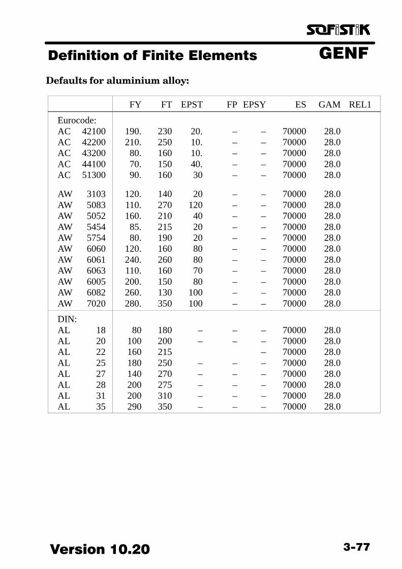
GENFDefinition of Finite Elements
3−77Version 10.20
Defaults for aluminium alloy:
FY FT EPST FP EPSY ES GAM REL1
Eurocode:AC 42100AC 42200AC 43200AC 44100AC 51300
AW 3103AW 5083AW 5052AW 5454AW 5754AW 6060AW 6061AW 6063AW 6005AW 6082AW 7020
190. 230 20. – – 70000 28.0210. 250 10. – – 70000 28.0 80. 160 10. – – 70000 28.0 70. 150 40. – – 70000 28.0 90. 160 30 – – 70000 28.0
120. 140 20 – – 70000 28.0110. 270 120 – – 70000 28.0160. 210 40 – – 70000 28.0 85. 215 20 – – 70000 28.0 80. 190 20 – – 70000 28.0120. 160 80 – – 70000 28.0240. 260 80 – – 70000 28.0110. 160 70 – – 70000 28.0200. 150 80 – – 70000 28.0260. 130 100 – – 70000 28.0280. 350 100 – – 70000 28.0
DIN:AL 18AL 20AL 22AL 25AL 27AL 28AL 31AL 35
80 180 – – – 70000 28.0100 200 – – – 70000 28.0160 215 – 70000 28.0180 250 – – – 70000 28.0140 270 – – – 70000 28.0200 275 – – – 70000 28.0200 310 – – – 70000 28.0290 350 – – – 70000 28.0
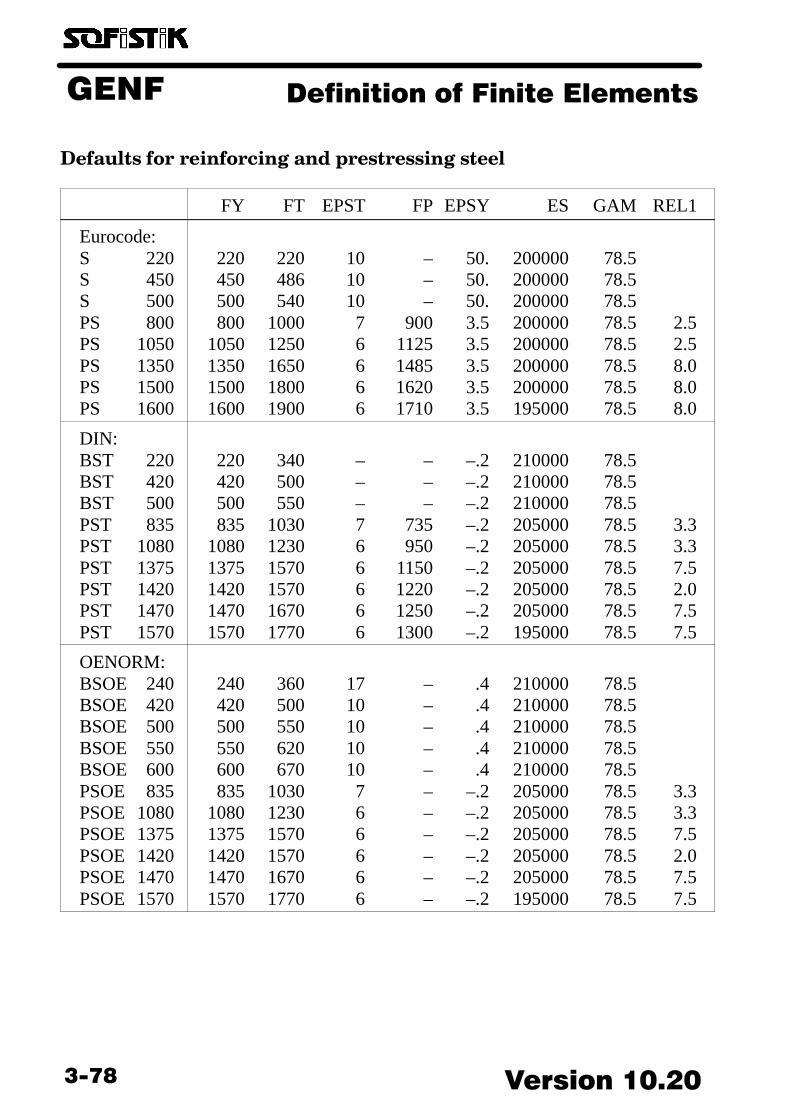
GENF Definition of Finite Elements
Version 10.203−78
Defaults for reinforcing and prestressing steel
FY FT EPST FP EPSY ES GAM REL1
Eurocode:S 220S 450S 500PS 800PS 1050PS 1350PS 1500PS 1600
220 220 10 – 50. 200000 78.5450 486 10 – 50. 200000 78.5500 540 10 – 50. 200000 78.5800 1000 7 900 3.5 200000 78.5 2.5
1050 1250 6 1125 3.5 200000 78.5 2.51350 1650 6 1485 3.5 200000 78.5 8.01500 1800 6 1620 3.5 200000 78.5 8.01600 1900 6 1710 3.5 195000 78.5 8.0
DIN:BST 220BST 420BST 500PST 835PST 1080PST 1375PST 1420PST 1470PST 1570
220 340 – – –.2 210000 78.5420 500 – – –.2 210000 78.5500 550 – – –.2 210000 78.5835 1030 7 735 –.2 205000 78.5 3.3
1080 1230 6 950 –.2 205000 78.5 3.31375 1570 6 1150 –.2 205000 78.5 7.51420 1570 6 1220 –.2 205000 78.5 2.01470 1670 6 1250 –.2 205000 78.5 7.51570 1770 6 1300 –.2 195000 78.5 7.5
OENORM:BSOE 240BSOE 420BSOE 500BSOE 550BSOE 600PSOE 835PSOE 1080PSOE 1375PSOE 1420PSOE 1470PSOE 1570
240 360 17 – .4 210000 78.5420 500 10 – .4 210000 78.5500 550 10 – .4 210000 78.5550 620 10 – .4 210000 78.5600 670 10 – .4 210000 78.5835 1030 7 – –.2 205000 78.5 3.3
1080 1230 6 – –.2 205000 78.5 3.31375 1570 6 – –.2 205000 78.5 7.51420 1570 6 – –.2 205000 78.5 2.01470 1670 6 – –.2 205000 78.5 7.51570 1770 6 – –.2 195000 78.5 7.5

GENFDefinition of Finite Elements
3−79Version 10.20
FY FT EPST FP EPSY ES GAM REL1
SIA:BSIA 235BSIA 500BSIA 550PSIA 830PSIA 1000PSIA 1410PSIA 1500PSIA 1590PSIA 1640PSIA 1670
220 360 25 – –.2 210000 78.5460 550 14 – –.2 210000 78.5520 580 8 – –.2 210000 78.5830 1030 6.5 – –.2 210000 78.5 3.3
1080 1230 6.5 – –.2 210000 78.5 3.31410 1570 6 – –.2 210000 78.5 1.81500 1670 5 – –.2 210000 78.5 7.51590 1770 5 – –.2 195000 78.5 7.51640 1820 5 – –.2 195000 78.5 7.51670 1860 5 – –.2 195000 78.5 7.5
BritishStandard:SBS 250SBS 460SBS 500PSBS 800PSBS 1050PSBS 1350PSBS 1500PSBS 1600
250 250 – – 200000 78.5460 460 – – 200000 78.5500 500 – – 200000 78.5800 1000 7 800 –.5 200000 78.5 2.5
1050 1250 6 1000 –.5 200000 78.5 2.51350 1650 6 1320 –.5 200000 78.5 8.01500 1800 6 1440 –.5 200000 78.5 8.01600 1900 6 1520 –.5 195000 78.5 8.0
ACI/AASHTO:SACI 40SACI 50SACI 60SACI 70SACI 75
280 490 – – 200000 78.5350 560 – – 200000 78.5420 630 – – 200000 78.5490 560 – – 200000 78.5520 600 – – 200000 78.5
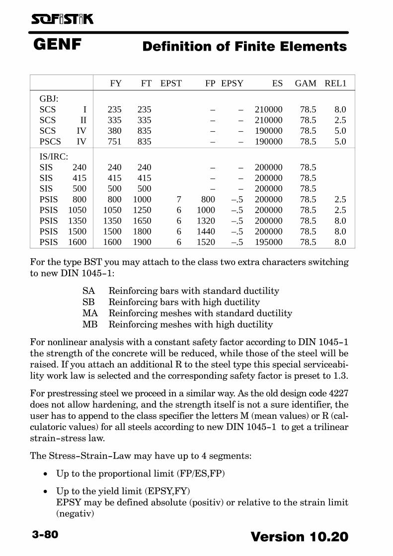
GENF Definition of Finite Elements
Version 10.203−80
FY FT EPST FP EPSY ES GAM REL1
GBJ:SCS ISCS IISCS IVPSCS IV
235 235 – – 210000 78.5 8.0335 335 – – 210000 78.5 2.5380 835 – – 190000 78.5 5.0751 835 – – 190000 78.5 5.0
IS/IRC:SIS 240SIS 415SIS 500PSIS 800PSIS 1050PSIS 1350PSIS 1500PSIS 1600
240 240 – – 200000 78.5415 415 – – 200000 78.5500 500 – – 200000 78.5800 1000 7 800 –.5 200000 78.5 2.5
1050 1250 6 1000 –.5 200000 78.5 2.51350 1650 6 1320 –.5 200000 78.5 8.01500 1800 6 1440 –.5 200000 78.5 8.01600 1900 6 1520 –.5 195000 78.5 8.0
For the type BST you may attach to the class two extra characters switchingto new DIN 1045−1:
SA Reinforcing bars with standard ductilitySB Reinforcing bars with high ductilityMA Reinforcing meshes with standard ductilityMB Reinforcing meshes with high ductility
For nonlinear analysis with a constant safety factor according to DIN 1045−1the strength of the concrete will be reduced, while those of the steel will beraised. If you attach an additional R to the steel type this special serviceabi�lity work law is selected and the corresponding safety factor is preset to 1.3.
For prestressing steel we proceed in a similar way. As the old design code 4227does not allow hardening, and the strength itself is not a sure identifier, theuser has to append to the class specifier the letters M (mean values) or R (cal�culatoric values) for all steels according to new DIN 1045−1 to get a trilinearstrain−stress law.
The Stress−Strain−Law may have up to 4 segments:
• Up to the proportional limit (FP/ES,FP)
• Up to the yield limit (EPSY,FY)EPSY may be defined absolute (positiv) or relative to the strain limit(negativ)

GENFDefinition of Finite Elements
3−81Version 10.20
• Up to the tensile strength (EPST,FT)
• constant to the infinite (1000 o/oo)
Depending on the steel class the values EPSY and EPST and FP will bepreset. With explicit definitions you may suppress:
• If FP is not lesser than FY the first part will be omitted.
• If EPST is not greater than EPSY the third part will be omitted.
More general work laws are specified via record SSLA.
In general the stress−strain laws are identical for servicability and ultimatelimit design. However for EC2 and DIN 1045−1 there are numerous explicitchanges. To select a prestressing steel according to DIN 1045−1, you have toselect the literal PS and append the characters DIN to the class value.
As the safety−factor concept will divide all stresses with the same safety fac�tor, the ultimate limit stress−strain−law will have an augmented initialmodulus if only the strength should be reduced.
Although the tensile strength for reinforcement steel with standard ductilitywill be reached at 25 o/oo, it is not allowed to use this in the design accordingto DIN 1045−1. The stress strain laws for design and nonlinear analysis differtherefore for those materials.

GENF Definition of Finite Elements
Version 10.203−82
The bond coefficients R of reinforcements and prestressing steel are input asreference values for environment condition 1. The values for other environ�ment conditions are controlled through factors during design in AQB. The de�faults are:
R K1
Reinforcing steelPrestressing stee
200150
0.82.0
The safety factor SCM is preset to 1.1 for steel materials. For reinforcing andprestressing steel it is preset to 1.15 resp. 1.05. The safety factor becomes ef�fective for the calculation of the full plastic internal forces of steel and com�posite sections.

GENFDefinition of Finite Elements
3−83Version 10.20
3.28. TIMB − Properties of Timber
ÖÖÖÖÖÖÖÖÖÖÖÖÖÖÖÖÖÖÖÖÖÖÖÖÖÖÖÖÖÖÖÖ
TIMB
Item Description Dimension Default
NOTYPE
CLAS
Material number (1−999)Type of material
see following tableQuality class (1−3 for NA, 1−2 for BS)
Strength by C and GL
−LIT
−
1NA
2
EPGE90QHQH90GAMALFASCMFMFT0FT90FC0FC90FVFVROALOAF
Elastic modulus parallel to fibreShear modulusElastic modulus normal to fibrePoisson’s ratio (polywood panels)Poisson’s ratio yz (solid wood)Unit weightTemperature elongation coefficientMaterial safety factorBending strengthTensile strength parallel to the fibreTensile strength normal to the fibreCompressive strength parallel to fibresCompressive strength normal to fibresShear strength at center (shear force)Shear strength at the edge (torsion)Meridian angle of anisotropyDescent angle of anisotropy
N/mm2
N/mm2
N/mm2
−−
kN/m3
�−
N/mm2
N/mm2
N/mm2
N/mm2
N/mm2
N/mm2
N/mm2
degreedegree
******
0.01.3*******
0.00.0
TITL Material designation Lit32 *

GENF Definition of Finite Elements
Version 10.203−84
Types and defaults:
TYPE (CLAS) EP G GAM Explanation
C * (27)GL * (27)NA 1
23
BS 1211141618
S 71013
MS 101317
LA –LB –LC –FTK –L –BE –
see EC5see EC510000 500 6
800011000 500 5
11000 550 511000 600 512000 650 513000 700 58000 500 610000 500 610500 500 610000 500 611500 550 612500 600 612500 1000 813000 1000 !17000 1000 !10000 500 611000 500 612000 1000 8
EC5 solid woodEC5 glued laminated woodDIN 1052 coniferous softwood
DIN 1052 glued laminated wood
DIN 1052 A–1 laminated wood
timber classes acc. DIN 4076
sorted timber classes DIN 4076
DIN 1052 deciduous hardwoodDIN 1052 deciduous hardwoodDIN 1052 deciduous hardwoodOeNORM B3001 spruce, fir, pineOeNORM B3001 larchOeNORM B3001 beech, oak

GENFDefinition of Finite Elements
3−85Version 10.20
3.29. MASO − Masonry / Brickwork
ÖÖÖÖÖÖÖÖÖÖÖÖÖÖÖÖÖÖÖÖÖÖÖÖÖÖÖÖÖÖÖÖ
MASO
Item Description Dimension Default
NOSTYP
SCLAMCLA
Material number (1−999)Type of brick stone
SB Standard solid BrickLS Limestone BrickLC Lightweight concreteC concreteCC cellular concreteBS British Standard 5628−1BS−2 Britisch Standard 5628−2
Strength of brick stoneGroup or strength of mortar
i,ii,iia,iii,iiia,iv Standard mortarDM Thin bed mortarLM21,LM36 Light mortarnumerical Qualified mortar
−LIT
N/mm2
LIT
N/mm2
1MZ
**
EGMUEGAMALFASCMFCNFCFTFVFHSFTB
Elastic modulusShear modulusPoisson’s ratioUnit weightTemperature elongation coefficientMaterial safety factorNominal strength σo
Compressive strengthTensile strengthShear strengthAdhesional shear strength βHS=2σoHS
Brick tensile strength βRZ
N/mm2
N/mm2
−kN/m3
�−
N/mm2
N/mm2
N/mm2
N/mm2
N/mm2
N/mm2
*****
2.5*
σo/0.35****
TITL Material name Lit32 *
As there are not yet any specific design routines, the parameters follow DIN1996−1−1 (EC6). According to DIN 1053−1 you should use a value of 2.5 forSCM and 2.67 so to FC. For masonry according to BS you have to attach thegroup A to D to the strength of the brick stone.

GENF Definition of Finite Elements
Version 10.203−86
For masonry according to BS 5628−1 the group A to D has to be a prefix to thestone class. You may then select the mortar designations I to IV. FT is the ten�sile strength for bending according Table 3 �parallel to bed joints", FV is thevertical shear strength according pict. 2 resp clause (25, part 2), FHS is thebasic shear value according clause 25 part 1, FTB is the bending tensilestrength according Table 3 �perpendicular to bed joints". FT and FTB varyconsiderably and should therefore be specified.
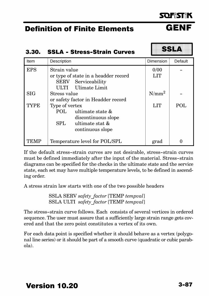
GENFDefinition of Finite Elements
3−87Version 10.20
3.30. SSLA − Stress−Strain Curves
ÖÖÖÖÖÖÖÖÖÖÖÖÖÖÖÖÖÖÖÖÖÖÖÖÖÖÖÖÖÖÖÖ
SSLA
Item Description Dimension Default
EPS
SIG
TYPE
TEMP
Strain valueor type of state in a headder record
SERV ServiceabilityULTI Ulimate Limit
Stress valueor safety factor in Headder recordType of vertex
POL ultimate state &discontinuous slope
SPL ultimate stat & continuous slope
Temperature level for POL/SPL
0/00LIT
N/mm2
LIT
grad
−
−
POL
0
If the default stress−strain curves are not desirable, stress−strain curvesmust be defined immediately after the input of the material. Stress−straindiagrams can be specified for the checks in the ultimate state and the servicestate, each set may have multiple temperature levels, to be defined in ascend�ing order.
A stress strain law starts with one of the two possible headers
SSLA SERV safety_factor [TEMP tempval]SSLA ULTI safety_factor [TEMP tempval]
The stress−strain curve follows. Each consists of several vertices in orderedsequence. The user must assure that a sufficiently large strain range gets cov�ered and that the zero point constitutes a vertex of its own.
For each data point is specified whether it should behave as a vertex (polygo�nal line series) or it should be part of a smooth curve (quadratic or cubic parab�ola).
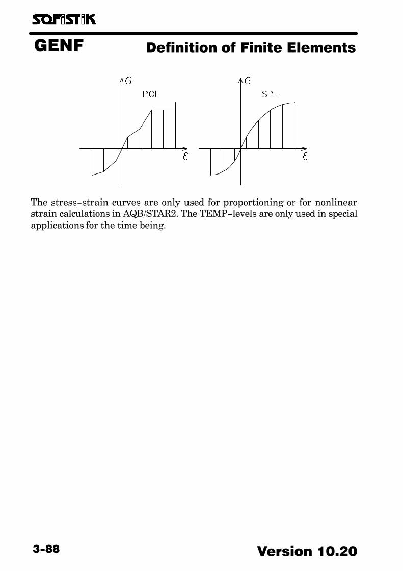
GENF Definition of Finite Elements
Version 10.203−88
The stress−strain curves are only used for proportioning or for nonlinearstrain calculations in AQB/STAR2. The TEMP−levels are only used in specialapplications for the time being.
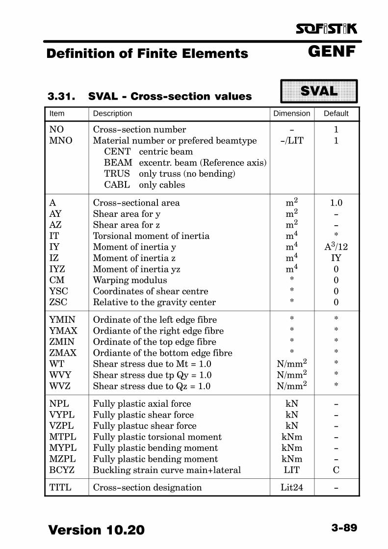
GENFDefinition of Finite Elements
3−89Version 10.20
3.31. SVAL − Cross−section values
ÖÖÖÖÖÖÖÖÖÖÖÖÖÖÖÖÖÖÖÖÖÖÖÖÖÖÖÖÖÖÖÖ
SVAL
Item Description Dimension Default
NOMNO
Cross−section numberMaterial number or prefered beamtype
CENT centric beamBEAM excentr. beam (Reference axis)TRUS only truss (no bending)CABL only cables
−−/LIT
11
AAYAZITIYIZIYZCMYSCZSC
Cross−sectional areaShear area for yShear area for zTorsional moment of inertiaMoment of inertia yMoment of inertia zMoment of inertia yzWarping modulusCoordinates of shear centreRelative to the gravity center
m2
m2
m2
m4
m4
m4
m4
***
1.0−−*
A3/12IY0000
YMINYMAXZMINZMAXWTWVYWVZ
Ordinate of the left edge fibreOrdiante of the right edge fibreOrdinate of the top edge fibreOrdiante of the bottom edge fibreShear stress due to Mt = 1.0Shear stress due tp Qy = 1.0Shear stress due to Qz = 1.0
****
N/mm2
N/mm2
N/mm2
*******
NPLVYPLVZPLMTPLMYPLMZPLBCYZ
Fully plastic axial forceFully plastic shear forceFully plastuc shear forceFully plastic torsional momentFully plastic bending momentFully plastic bending momentBuckling strain curve main+lateral
kNkNkN
kNmkNmkNmLIT
−−−−−−C
TITL Cross−section designation Lit24 −
GENF Definition of Finite Elements
Version 10.203−90
This command allows the input of cross−sections without the correspondinggeometric data, which are necessary of course in detailed stress analysis,yield zone theory or reinforced concrete dimensioning. They can be used in thestatic analysis or simplified checks with full plastic internal forces.
With NO and a Literal for MNO you may also specify which element typeshould be selected for automatic elements whith that section. This definitioncan be redone at any time for any section. All other input values will be igno�red in that case.
Plastic internal forces may be needed for cross−sections with trial values. Itis explicitly stated, however, that the use of this input command for dimen�sioning is by no means in accordance with the intentions of the program’sauthor for a consistent data input, and the user bears the sole responsibilityin this case.
If IT is defined zero, special attention should be paid so that the torsional de�gree of freedom during the assembly of the total static system does not leadto undefined rotation capability (Error message: Parts of the system canmove freely.).
The default for IY is equivalent to a rectangular section with a width of 1 mand the given area A.
In accordance with Saint Venant’s estimate, the default value for the tor�sional moment of inertia is
)II(4A
Izy
2
4
T +⋅Π⋅=
This value is exact for circular and elliptical sections.
Deviations for a rectangular section:
a/b 1/1 2/1 10/1
exact 0.140 0.458 3.13
approx. 0.152 0.486 3.01
The defaults for ymin down to zmax start from a rectangular cross−sectionand they are derived by appropriate corrections from the radius of gyration.
The default values for the full plastic internal forces come out of the cross−sec�tional area. WT enters the default for MTPL, while MYPL and MZPL makeuse of the extreme coordinates ymin through zmax.

GENFDefinition of Finite Elements
3−91Version 10.20
All full plastic internal forces are without safety factor.
In the case of the buckling strain lines the literals 0,A,B,C,D are used for thesame curves in the main and the lateral direction and AB, BC and CD for dif�ferent curves.
SVAL can make an identical copy of an already defined cross−section by in�putting SVAL NEWNO−OLDNO. This serves in accelarating the method,when different cross−section values must be applied later on.
SVAL can also be used for defining a reduced cross section. This can be doneeither by using a negative NO to modify an already defined cross−section, orby making a copy of an existing cross−section by means of a negative MNO.The values A through ZSC are then viewed as factors for the correspondingvalues, and are thus preset to 1.0. The new cross−section has no geometricproperties any more.
Example:
PROF 1 HEB 300PROF 2 HEB 300SVAL −1 IT 0.5SVAL 3 −2 IT 0.5SECT 4; SV IT −0.5 ; PROF 1 HEB 300
Cross−section 1 receives 50% of the torsional moment of inertia. The ge�ometry of the cross−section gets erased. Cross section 3 has 50% of the tor�sional moment of inertia of cross−section 2, has no geometry, and is henceidentical to cross−section 1. Cross−section 2 was not modified. Cross−section4 is a cross−section with IT reduced by half and with complete geometry.(Only possible with AQUA)

GENF Definition of Finite Elements
Version 10.203−92
3.32. SREC − Rectangle, T−beam,
Plate
ÖÖÖÖÖÖÖÖÖÖÖÖÖÖÖÖÖÖÖÖÖÖÖÖÖÖÖÖÖÖÖÖÖÖÖÖ
SREC
Item Description Dimension Default
NOHBHOBOSOSUASOASU
Cross section numberTotal heightWidth for rectangular, T−beamThickness of the plate (upper part)Thickness of the plate (lower part)Inset of top reinforcementInset of bottom reinforcementMinimum top reinforcement− layer 2Minimum bottom reinforcement − layer 1
−****
cmcmcm2
cm2
1−
1m00
H/10SO00
MNOMRF
RTYP
ITSAYSAZDASODASUREF
TITL
Material numberMaterial number of reinforcement
+1000 ⋅ material stirrup reinforcementReinforcement subtype
ASYM = assymmetric two sidedASYT = assymetric three sidedSYM = symmetricalSYMT = symm.+ along the sidesCU = perimetric reinforcement
Factor for torsional moment of inertiaShear area for VYShear area for VZDiameter of top reinfrocementDiameter of bottom reinforcementLocation of zero point
C = gravity centerR/L/M = right / left / middleUR/UL/UM = upper right/left/middleLR/LL/LM = lower right/left/middlePR/PL/PM = plate right/left/middle
Cross−section designation
−−
LIT
−/m4
−/m2
−/m2
mmmmLIT
Lit32
**
*
−1.0.0.28
DASOC
*
Depending on the definition of values one of the following types of section isgenerated:

GENFDefinition of Finite Elements
3−93Version 10.20
H Plate with implied width of 1 m or width BOH,B Rectangular cross sectionH...BO T−Beam cross section
Following this classification different design codes will be applied to the sec�tions.
When nothing is input for REF, the zero point of the coordinate system of thecross−section is assumed to be at the gravity center.
The required dimensions of the cross−section can be calculated by AQB. Forthis task, B or H can be input negative when only that dimension should bechanged.
The full height of the web and the entire plate are used in determining thetorsional moment of inertia and the torsional shear stresses; for the equival�ent hollow cross−section used in computing the torsion reinforcement onlythe web or only the plate is used, depending on which part is larger. The checkof the shear stress due to shear force takes place at the most unfavourablelocation (at the height of the gravity center for the web or at the intersectionof web and plate). For the interests of massive constructions the effective tor�sional moment of inertia can be reduced by IT. The input of a positive valuespecifies a value in m4, while a negative value is interpreted as a factor.

GENF Definition of Finite Elements
Version 10.203−94
Shear areas are typically not used. They can be defined, however, by specify�ing SAY or SAZ. The input of a positive value specifies a value in m2, whilea negative value is interpreted as a factor for the default value of the rec�tangular cross−section and the web or the plate.
The lower reinforcement is layer 1, the upper one is layer 2. If the distanceof the reinforcements is greater than 30 cm, addititonal reinforcement at theside of the web will be introduced with layer number 3. As it is only neededfor torsion, you might suppress this by entering a value for RTYP or a zerovalue for IT. If not suppressed it might be activated for ultimate design inbiaxial bending. Further we introduce a reinforcement at the lower side of theplate with layer number 4 if the upper layer is within the topmost quarter ofthe plate height.
At RTYP there are various items available:ASYT three layers (1,2,3) at lower, upper, midsidesASYM two layers (1,2) at lower and upper sideSYMT layer 0 at upper and lower side, layer 3 at midsideSYM only layer 0 at upper and lower sideCU layer 0 at all 4 sides (circumperipheral)CU0 as CU but without minimum shear reinforcementASY0,SYM0 ASYM,SYM without minim. shear reinforcementAST0,SYT0 ASYT,SYMT without minim. shear reinforcement
For symmetric reinforcement we have ASO applied for upper and lower sidewith layer 0, while layer 3 will be the optional torsional reinforcement at thesides. If CU is input, perimetric reinforcement gets generated. STB uses onlythe option SYM for ASO/ASU.
MRF = 0 must be specified for unreinforced cross−sections. The input of MRFis not allowed for steel or wooden cross−sections. When MRF is specified tobe smaller than 1000, the same material type will be assumed for the stirrupreinforcement as for the longitudinal one.
The cover of the reinforcement from the side edge is equal to the cover fromthe upper or lower edge, but not larger than one−fourth of the width.

GENFDefinition of Finite Elements
3−95Version 10.20
3.33. SCIR − Circular and Annular
Sections
ÖÖÖÖÖÖÖÖÖÖÖÖÖÖÖÖÖÖÖÖÖÖÖÖÖÖÖÖÖÖÖÖ
SCIR
Item Description Dimension Default
NORARISASIASA
ASI
Cross–section numberOuter radiusInner radiusOuter reinforcement inset (default: (ra–ri)/10)Inner reinforcement insetOuter reinforcement
(positive values in cm2/m)(negative values in cm2)
Inner reinforcement(omitted if nothing is input)
−mmcmcm*
*
1�0*
SA−
−
MNOMRF
ITFDAS
Material number of cross–sectionMaterial number of reinforcement
+ 1000 ⋅ material of stirrup reinforcementFactor for torsional moment of inertiaDiameter of reinforcement
−−
−mm
**
128
TITL Cross–section designation Lit32 *
Shear deformations are not considered.
Circular cross section

GENF Definition of Finite Elements
Version 10.203−96
3.34. BORE − Bore Profile of a
Sondation
ÄÄÄÄÄÄÄÄÄÄÄÄÄÄÄÄÄÄÄÄÄÄÄÄÄÄÄÄÄÄÄÄÄÄÄÄ
BORE
Item Description Dimension Default
NR
XYZ
NXNYNZ
ALFTITL
Number of bore profile
Coordinates of start point
Direction of bore profile Default: in gravity direction
Rotation angle of local axisTitle of bore profile
−
mmm
−−−
degreeLIT32
1
0.00.00.0
***
0.0*
With BORE we define a bore profil to be used for HASE and PFAHL to de�scribe the strata data of the soil.

GENFDefinition of Finite Elements
3−97Version 10.20
3.35. BLAY − Layer of the Soil Strata
ÄÄÄÄÄÄÄÄÄÄÄÄÄÄÄÄÄÄÄÄÄÄÄÄÄÄÄÄÄÄÄÄ
BLAY
Item Description Dimension Default
SMNOICEX
MNORICRE
HWMIHWMA
Ordinate along the profile axis (depth)Material number from this ordinate onConstruction stage for excavation
Materialnumber of refillConstruction stage for refill
Minimum ground water height Maximum griund water height
m
mm
*
0.00.0
With BLAY you may specify the geological strata data including the construc�tion phases "excavation" and "backfill".
All data is not yet used by any SOFiSTiK−Program.
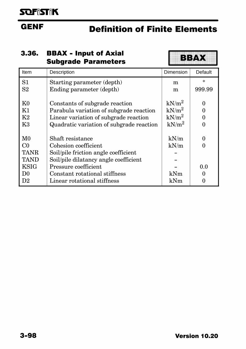
GENF Definition of Finite Elements
Version 10.203−98
3.36. BBAX − Input of Axial
Subgrade Parameters
ÄÄÄÄÄÄÄÄÄÄÄÄÄÄÄÄÄÄÄÄÄÄÄÄÄÄÄÄÄÄÄÄÄÄÄÄ
BBAX
Item Description Dimension Default
S1S2
K0K1K2K3
M0C0TANRTANDKSIGD0D2
Starting parameter (depth)Ending parameter (depth)
Constants of subgrade reactionParabula variation of subgrade reactionLinear variation of subgrade reactionQuadratic variation of subgrade reaction
Shaft resistanceCohesion coefficientSoil/pile friction angle coefficient Soil/pile dilatancy angle coefficientPressure coefficientConstant rotational stiffnessLinear rotational stiffness
mm
kN/m2 kN/m2 kN/m2 kN/m2
kN/mkN/m
−−−
kNmkNm
*999.99
0000
00
0.000
GENFDefinition of Finite Elements
3−99Version 10.20
3.37. BBLA − Input of Lateral
Subgrade Parameters
ÄÄÄÄÄÄÄÄÄÄÄÄÄÄÄÄÄÄÄÄÄÄÄÄÄÄÄÄÄÄÄÄ
BBLA
Item Description Dimension Default
S1S2
K0K1K2K3
P0P1P2P3
PMA1PMA2
Starting parameter (depth)Ending parameter (depth)
Constants of subgrade reaction Parabula variation of subgrade reactionLinear variation of subgrade reactionQuadratic variation of subgrade reaction
Factors for variation along the periphery
maximum foundation value at S1maximum foundation value at S2
mm
kN/m2 kN/m2 kN/m2 kN/m2
−−−−
kN/m2 kN/m2
*999.99
0000
1111
−−
Elastic support has many related parameters. That is why those values arecombined to special property elements for a geometric line.
All the corresponding GLBA and GLBL records follow the GLN record in theorder defined by the s ordinate. All data for the s ordinate refer to the para�metric system of coordinates which defaults to the global z− axis.
Within a section the subgrade modulus is interpolated by:
K�K0�K1�� z� z1z2 � z1
�1�2
�K2� � z� z1z2� z1
��K3�� z� z1z2 � z1
�2
The subgrade modulus at the beginning of the section is K0, and the one atits end is K0+K1+K2+K3. The discrete values correspond to constant, para�bolic, linear and quadratic distributions.
The default value for S1 is the latest S2 value. The initial default is −999.99.The factors for the variation along the periphery are effective at the angle (0,90, 180 and 270 degrees). The angle is measured against the local z−axis. Inlinear analysis the factor (P0+P2)/2 is used for the primary bending (MY,VZ),while (P1+P3)/2 is used for the secondary bending (MZ,VY).

GENF Definition of Finite Elements
Version 10.203−100
For the axial reaction a rather sophisticated approach is available. The pres�sure allowing frictional support has many sources.
�� ��KSIG� �v�K(x)� �v(x) �TAND�u(x)�
�� ��K(x)�u(x)� ��TANR� ��C0
The first part of the pressure is given by the vertical earth pressure and thehorizontal pressure coefficient. The second part is given by the elastic con�stants of the lateral stiff− ness and a combination of the displacements.
GENFDefinition of Finite Elements
3−101Version 10.20
See also: BEAM
3.38. HING − Hinged Connection
Combinations for Beams
ÄÄÄÄÄÄÄÄÄÄÄÄÄÄÄÄÄÄÄÄÄÄÄÄÄÄÄÄÄÄÄÄ
HING
Item Description Dimension Default
NO
G1G2G3G4G5G6
Number of definition (max. 10)
Up to 6 from the following literals can beentered making the corresponding inter�nal forces equal to zero.
N VY VZ MT MY MZ MB
−
LITLITLITLITLITLIT
1
−−−−−−
Simple hinge actions can be entered directly for beams too.

GENF Definition of Finite Elements
Version 10.203−102
See also: SYST, MESH, MAT, BEAM, QUAD, BRIC, SPRI, TRUS, CABL
3.39. GRP − Group ControlÄÄÄÄÄÄÄÄÄÄÄÄÄÄÄÄÄÄÄÄÄÄÄÄÄÄÄ
GRP
Item Description Dimension Default
NOGT
MNO
MRF
STI
NR
POSI
TXTYTXY
TD
Group numberThickness of QUAD−elements
Material numberThe default is the lowest materia numberthat does not represent any reinforce�ment.Material number of the reinforcementThe default is the lowest materialnumber of any reinforcement in the data�base.
Element formulation (refer to QUAD)0 = geometry only1 = plate action2 = membrane action3 = in−plane bending
Direction of the local a−axis (refer toQUAD)Element position w.r.t. the nodes (refer toQUAD)
CENT Element lies centred w.r.t. thenodes
ABOV Element lies above the nodesBELO Element lies below the nodes
Thickness in local x−direction (QUAD)Thickness in local y−directionThickness for lateral bending (refer toSEPP)Thickness for torsion (refer to SEPP)
MIN−T = minimum of TX and TY
−
m/*
−
−
−
LIT
LIT
m/*m/*m/*
m/*
!
0.2
*
*
*
−
CENT
TT
MIN−T
MIN−T
GENFDefinition of Finite Elements
3−103Version 10.20
This is an attribute record. All elements input after it receive the currentgroup provided that they are not categorized explicitly differently.
The group number of an element is calculated by dividing the elementnumber by the group divisor. The maximum group number amounts to 999.
Beispiele:Gruppendivisor ElementnummerGruppennummer
1000 1 01000 3569 32000 3569 1
5 3569 713
Examples:Group divisor Element number Group number
1000 1 01000 3569 32000 3569 1
5 3569 713
With the specification of a group classification in the sentence SYST group 0is preset. The input of GRP causes all following elements of the group 0 to bemoved to the specified group by an appropriate change of their elementnumber. The explicit input of elements with a group number deviating fromthe above is not reminded in order to maintain compatibility with old inputdata.
If nothing different is input by the QUAD record, the subsequent QUAD− el�ements are assigned the properties defined by this record.
The following restrictions hold for the input to TX through TD:
TX and TY can have different values compared to T.
The thickness T is used for the calculation of the gravity load always.
The thicknesses TX through TD are used for orthotropic analysis. De�tailed analysis principles can be found in the particular program de�scriptions (SEPP, TALPA).
The orthotropic thicknesses are rotated along through the input of andorthotropy angle OAL by the MAT record!

GENF Definition of Finite Elements
Version 10.203−104
If a different value is input for the thickness T by the QUAD record, the ortho�tropic thicknesses of the GRP record for this element get multiplied by thefactor T−QUAD / T−GRP.
The material number is provided as general option. An explicit input by el�ements as well as by MESH or IMES takes precedence.
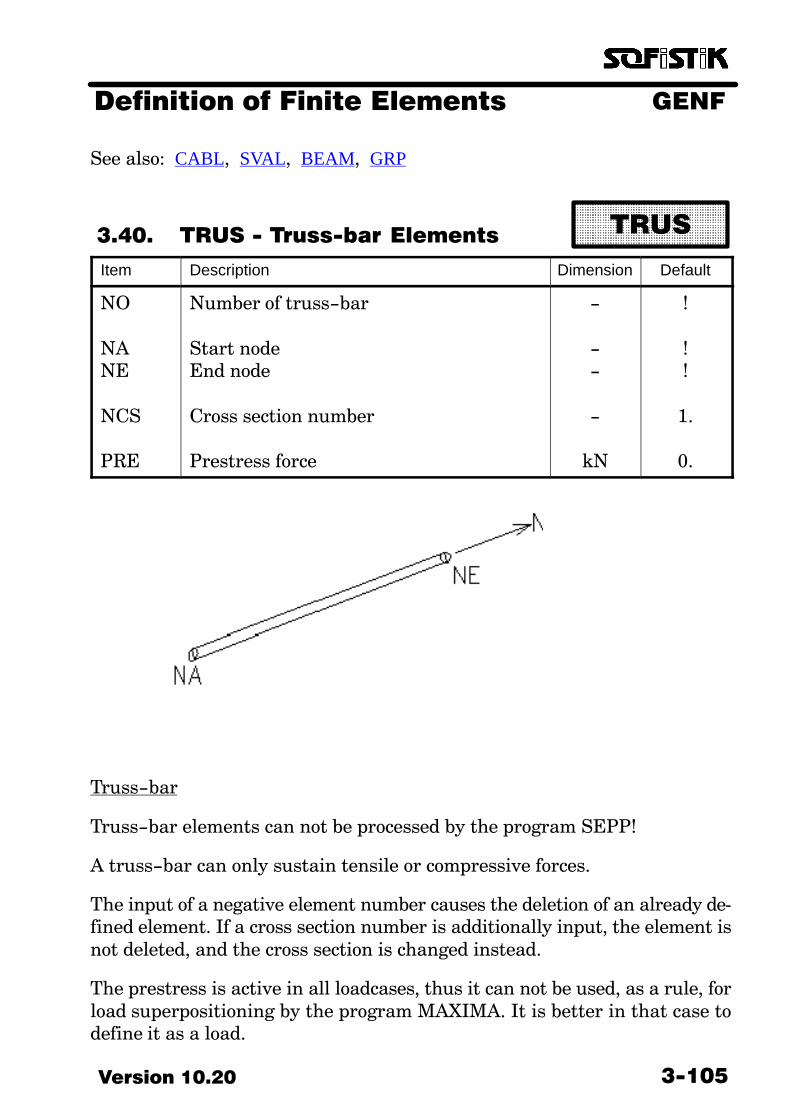
GENFDefinition of Finite Elements
3−105Version 10.20
See also: CABL, SVAL, BEAM, GRP
3.40. TRUS − Truss−bar Elements
ÄÄÄÄÄÄÄÄÄÄÄÄÄÄÄÄÄÄÄÄÄÄÄÄÄÄÄÄÄÄÄÄ
TRUS
Item Description Dimension Default
NO
NANE
NCS
PRE
Number of truss−bar
Start nodeEnd node
Cross section number
Prestress force
−
−−
−
kN
!
!!
1.
0.
Truss−bar
Truss−bar elements can not be processed by the program SEPP!
A truss−bar can only sustain tensile or compressive forces.
The input of a negative element number causes the deletion of an already de�fined element. If a cross section number is additionally input, the element isnot deleted, and the cross section is changed instead.
The prestress is active in all loadcases, thus it can not be used, as a rule, forload superpositioning by the program MAXIMA. It is better in that case todefine it as a load.
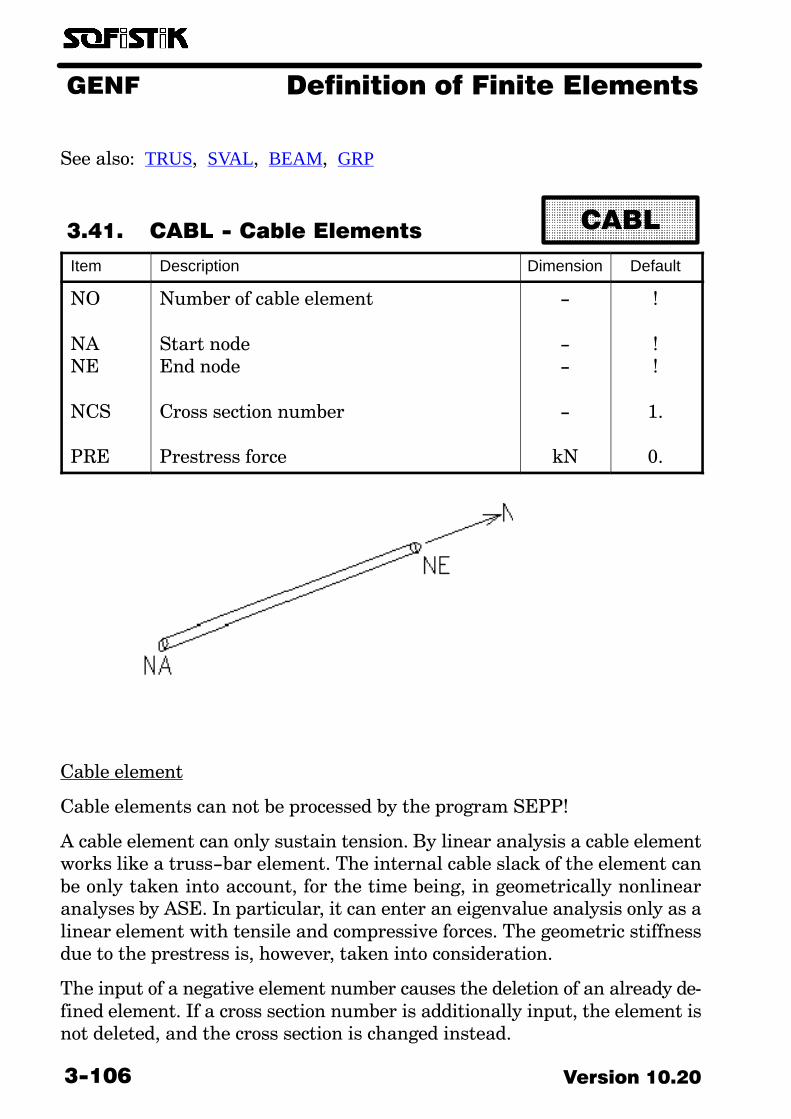
GENF Definition of Finite Elements
Version 10.203−106
See also: TRUS, SVAL, BEAM, GRP
3.41. CABL − Cable Elements
ÄÄÄÄÄÄÄÄÄÄÄÄÄÄÄÄÄÄÄÄÄÄÄÄÄÄÄ
CABL
Item Description Dimension Default
NO
NANE
NCS
PRE
Number of cable element
Start nodeEnd node
Cross section number
Prestress force
−
−−
−
kN
!
!!
1.
0.
Cable element
Cable elements can not be processed by the program SEPP!
A cable element can only sustain tension. By linear analysis a cable elementworks like a truss−bar element. The internal cable slack of the element canbe only taken into account, for the time being, in geometrically nonlinearanalyses by ASE. In particular, it can enter an eigenvalue analysis only as alinear element with tensile and compressive forces. The geometric stiffnessdue to the prestress is, however, taken into consideration.
The input of a negative element number causes the deletion of an already de�fined element. If a cross section number is additionally input, the element isnot deleted, and the cross section is changed instead.

GENFDefinition of Finite Elements
3−107Version 10.20
The prestress is active in all loadcases, thus it can not be used, as a rule, forload superpositioning by the program MAXIMA. It is better in that case todefine it as a load.

GENF Definition of Finite Elements
Version 10.203−108
See also: ADEF, HING, BSEC, SVAL, GRP
3.42. BEAM − Beam Elements
ÄÄÄÄÄÄÄÄÄÄÄÄÄÄÄÄÄÄÄÄÄÄÄÄÄÄÄÄÄÄÄÄÄÄÄÄ
BEAM
Item Description Dimension Default
NO
NANE
NR
NCS
AHINEHIN
DIV
NBD
NPNCSE
Element number
Number of start beam nodeNumber of end beam node
Direction data of Y−axis(parameter omitted by plane systems)
Cross section number
Input of hinge at start nodeInput of hinge at end node
Partitioning of beam into DIV (<50)equal segments with the same cross sec�tion number
Number of segment definition
Geometry or foundation numberCross section number at beam end
−
−−
LIT/degrees
−
−/LIT−/LIT
−
−
−−
!
!!
0
1
**
1
−
−NCS
A beam element is defined through two nodes and a sectional description(NCS/NCSE). The records SUPP, BSEC and ADEF/BDIV can be used to de�scribe any desired variation of cross section. In this case it is to be ensuredno rotation of the main axis is allowed along the beam axis.
A uniform partitioning can be defined by DIV in case of prismatic beams. Ifa negative DIV is input, the segments acquire the attribute PRIN NO (seeADEF). With haunched beams definition of sections are necessary for everybeam section.
The input of a beam record with a negative element number causes the dele�tion of a previously defined element. If a cross section number is additionally

GENFDefinition of Finite Elements
3−109Version 10.20
input, the cross section is simply changed instead. A subsequent definition ofhaunches is no more possible in such case.
By AHIN and EHIN one can either enter the number of a hinge combinationthat has already been defined with HING or enter directly up to two of thefollowing hinge support conditions (without spaces in between):
N VY VZ MT MY MZ MB (Default: no hinges)
A pile element whose attributes with the profile or the GLN NP are definedis made by input of NP > 0. If NP is −1 a referenced beam element is generated.The axis of the beam is then the connection of the origin of the sectionalcoordinate system!
Beam coordinate system
Each beam or pile has a local system of coordinates x, y, z (refer to section 2.2).The longitudinal axis of the beam NA−NE defines the positive x−direction.The following cases can be distinguished regarding the orientation of theother two axes:
1. Plane frame
The structure lies in the global XY−plane. The local y−axis of the beam is par�allel to the global Z−axis but in the opposite direction. The local z−axis is per�pendicular to the axis of the beam and to the right of the direction of the beam.
2. Gridwork
The structure lies in the global XY−plane. The local z−axis is parallel to theglobal Z−axis. The local y−axis is perpendicular to the axis of the beam andto the right of the direction of the beam.

GENF Definition of Finite Elements
Version 10.203−110
3. Space frame
In a three−dimensional system the orientation of the local y−axis must be de�fined by the user. The parameter NR is available for this purpose. The localz−axis is perpendicular to the local x− and y−axes. Its direction is determinedby the three−finger right hand rule.
The following possibilities exist:
3.1. NR=0 (Default)
The local y−axis is parallel to the global XY−plane and perpendicular to theaxis of the beam, thus to the right of the direction of the beam. This is inde�pendant of the gravity direction always clockwise with respect to the globalZ−axis.

GENFDefinition of Finite Elements
3−111Version 10.20
Standard orientation
In case the axis of the beam is parallel to the global Z−axis, then the local z−axis is parallel to the global y−axis.
Special cases of orientation
3.2. NR negative (<0)
A negative value for NR is interpreted as an angle in degrees, by which thecoordinate system resulting from NR = 0 (refer to 3.1) must be rotated aboutthe axis of the beam. (A negative value is an angle rotating to the left, a posi�tive value is a direction node!)
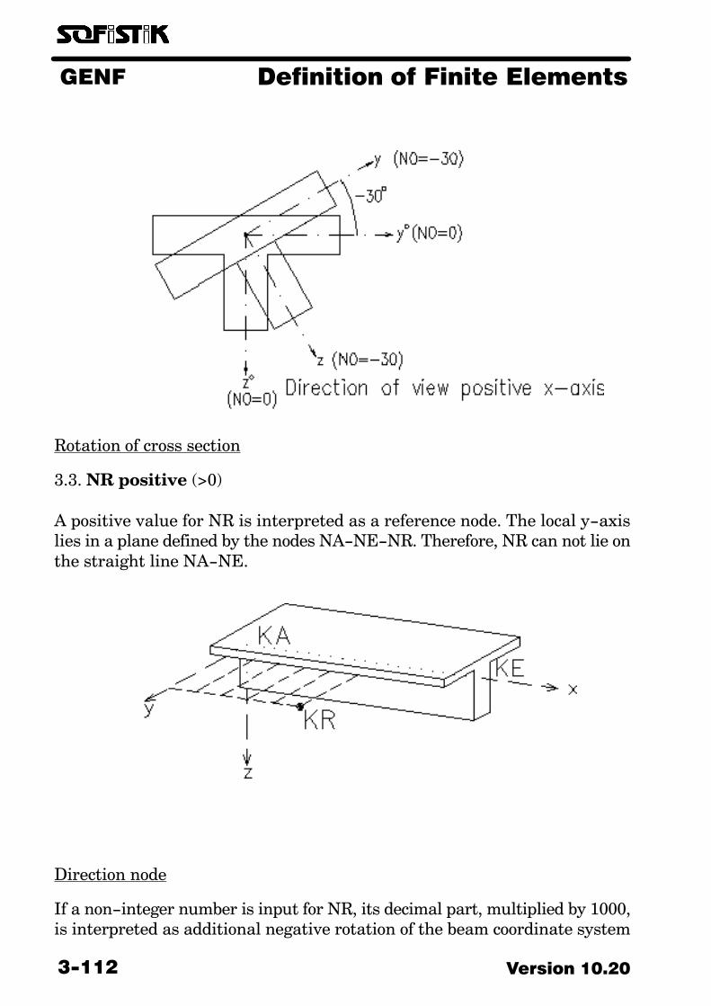
GENF Definition of Finite Elements
Version 10.203−112
Rotation of cross section
3.3. NR positive (>0)
A positive value for NR is interpreted as a reference node. The local y−axislies in a plane defined by the nodes NA−NE−NR. Therefore, NR can not lie onthe straight line NA−NE.
Direction node
If a non−integer number is input for NR, its decimal part, multiplied by 1000,is interpreted as additional negative rotation of the beam coordinate system

GENFDefinition of Finite Elements
3−113Version 10.20
about the beam axis in degrees. Thus, 5.090 rotates the z−axis in the planedefined by node 5.
3.4. NR as a literal
If one of the literals XX, YY, ZZ, NEGX, NEGY or NEGZ is input for NR thelocal y−axis will be placed on a plane defined by the axis of the beam and thecoordinate axis corresponding to that literal.
Haunches and sections
Beams can have segments and variable cross sections. Not all of the programsthough can take into consideration all the effects resulting from that. Onemust occasionally settle with an average value (e.g. rotation of the principalaxes or shear center).
Haunches can be defined in simple cases by a special input format for NCS.Namely, if a decimal number is entered for NCS (e.g. 1.02), the two decimaldigits define the cross section at the end of the beam element (1.2 describescross sections 1 and 20!). The parameter NCSE must be used in case of threedigit cross section numbers.
The user generally has a whole range of input options. Combinations are al�lowed, but duplicate section definitions are usually ignored.
1. Input of DIVThe beam is partitioned into an integer number of parts. Each sec�tion acquires the cross section number of its predecessor. Beams withhaunches therefore can not be partitioned this way.
2. ADEF and BDIV can define a pattern of segment lengths and crosssection numbers, which can be suited upon several beams through ascaling of the individual segment lengths or the sum of them. Crosssection jumps can be solely defined by means of this method.
3. Input of SUPPThe use of SUPP generates the sections that are usually necessary fora check (edge of support and critical section for shear).
4. Input of BSECIt can be used for explicit section definitions.
The output or the proportioning of internal section forces is usually possibleonly for cross sections specified by a segment definition or a partitioning. Fornonlinear analysis it is necessary to define a large number of sections.
GENF Definition of Finite Elements
Version 10.203−114
All sections can include additional information for controlling the processingof the sections during the proportioning and the static analysis. Two para�meters are provided for this purpose:
STYP Typ des Schnitts
ABSC Normaler SchnittANSC Anschnitt eines biegesteifen AnschlussesAGEL Anschnitt eines Auflagers mit gelenkigem Anschluß
(Mauerwerk)AIND Anschnitt eines indirekten AuflagersSCHU Für die Schubbemessung maßgebender Schnitt
STYP Type of section
SECT Regular sectionFACE Section at the face of a clamped connectionHFAC Section at the face of a support with articulated
connection (masonry)IFAC Section at the face of an indirect supportSHEA Critical section for shear proportioning
and
PRIN Ausgabekategorie des Schnittes
JA Schnitt wird immer ausgegebenNEIN Schnitt wird nur gedruckt, wenn eine entsprechende
ECHO−Option gesetzt ist.
PRIN Output category of the section
YES Section data will be output alwaysNO Section data will be output only when a corresponding
ECHO−option is set.
RICH Richtung von STYP
HAUP Hauptrichtung (Vz,My)QUER Querrichtung (Vy,Mz)VOLL Beide Richtungen
GENFDefinition of Finite Elements
3−115Version 10.20
DIRE Direction of STYP
MAIN Principal direction (Vz,My)TRAN Transverse direction (Vy,Mz)BOTH Both directions
ORT Lokalisierung des Schnitts
ANFA zum Stabanfang gehörendENDE zum Stabende gehörend
LOC Localization of the section
BEG belongs to beginning of beamEND belongs to end of beam
An assignment of the section to the beginning or the end of the beam is necess�ary for support sections, when these lie on the wrong side with respect to themidpoint of the beam. This is, for example, a case when a beam should besubdivided into more elements. The ’beginning’ then of the third beam el�ement could lie short of the beams end.
GENF Definition of Finite Elements
Version 10.203−116
See also: BDIV, BEAM, BSEC
3.43. ADEF − Beginning of Beam
Segment Definition
ÄÄÄÄÄÄÄÄÄÄÄÄÄÄÄÄÄÄÄÄÄÄÄÄÄÄÄÄÄÄÄÄÄÄÄÄ
ADEF
Item Description Dimension Default
NO Number of definition − 1
Up to 99 segment definitions can be entered. A segment definition consistsof one ADEF record and any number of BDIV records. It can describe one ormore entire beams. The same segment definition can be used for beams withdifferent lengths. The length adjustment is carried out according to one of twomethods:
1. None of the segment lengths DS is negative.The segment definition is built by measuring the lengths from thecentre of the beam.
2. At least one segment has a negative length.All other segment lengths are the same except for the negativelengths, which are adjusted so that the sum of the segmentlengths will equal the total beam length.
SUPP and BSEC are independent of ADEF and they can be defined in addi�tion to ADEF. The sections that are generated this way get sorted into ADEFin order to prevent duplicate definitions.
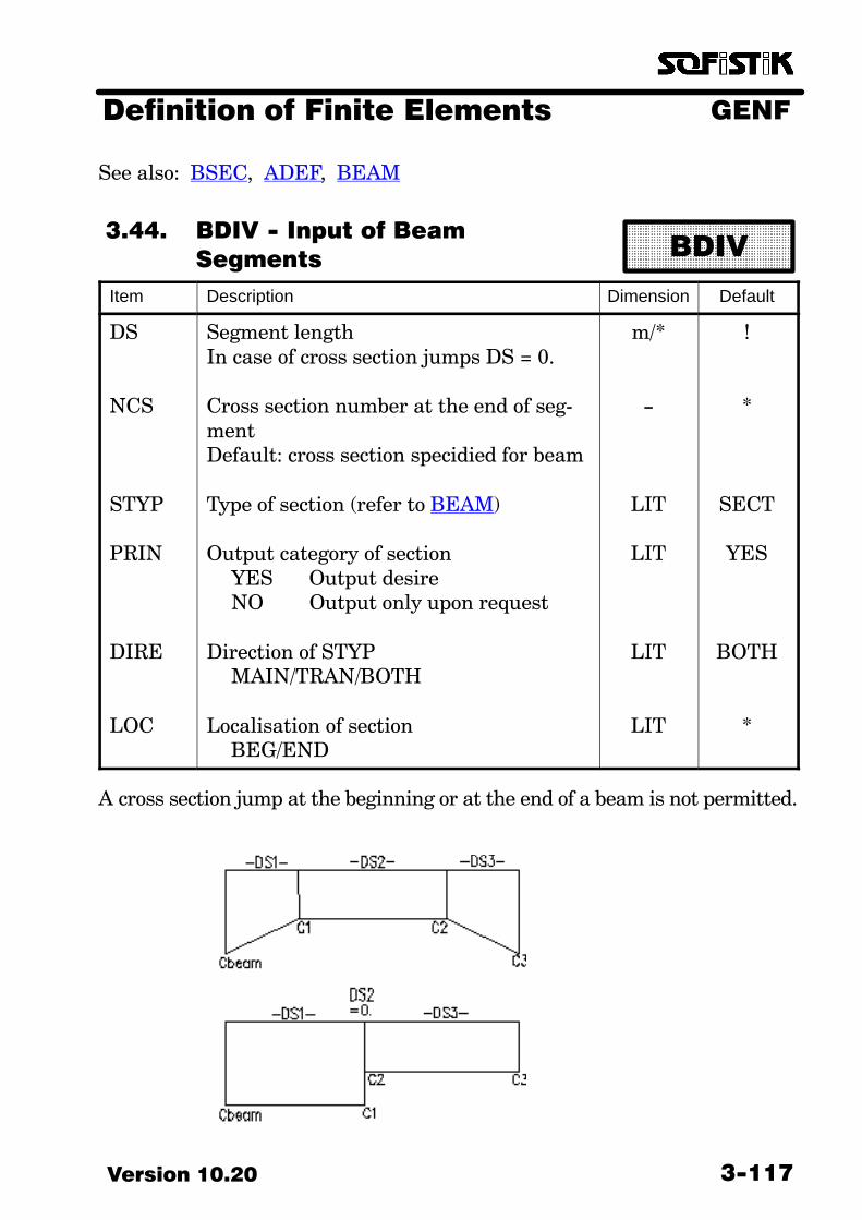
GENFDefinition of Finite Elements
3−117Version 10.20
See also: BSEC, ADEF, BEAM
3.44. BDIV − Input of Beam
Segments
ÄÄÄÄÄÄÄÄÄÄÄÄÄÄÄÄÄÄÄÄÄÄÄÄÄÄÄÄÄÄÄÄ
BDIV
Item Description Dimension Default
DS
NCS
STYP
PRIN
DIRE
LOC
Segment lengthIn case of cross section jumps DS = 0.
Cross section number at the end of seg�mentDefault: cross section specidied for beam
Type of section (refer to BEAM)
Output category of sectionYES Output desireNO Output only upon request
Direction of STYPMAIN/TRAN/BOTH
Localisation of sectionBEG/END
m/*
−
LIT
LIT
LIT
LIT
!
*
SECT
YES
BOTH
*
A cross section jump at the beginning or at the end of a beam is not permitted.

GENF Definition of Finite Elements
Version 10.203−118
Segment definition

GENFDefinition of Finite Elements
3−119Version 10.20
See also: BDIV, ADEF, BEAM
3.45. BSEC − Beam Sections
ÄÄÄÄÄÄÄÄÄÄÄÄÄÄÄÄÄÄÄÄÄÄÄÄÄÄÄÄÄÄÄÄ
BSEC
Item Description Dimension Default
NOXNCS
STYP
PRIN
DIRE
LOC
Beam numberSection locationCross section numberDefault: last cross section number
Type of section (refer to BEAM)
output category of sectionYES Output desiredNO Output only upon request
Direction of STYPMAIN/TRAN/BOTH
Localisation of sectionBEG/END
−m/*−
LIT
LIT
LIT
LIT
!!*
SECT
YES
BOTH
*
BSEC can be used, in addition to DIV and BDIV, to define sections in beamsfor output or dimensioning purposes.
GENF Definition of Finite Elements
Version 10.203−120
See also: BDIV, ADEF, BEAM
3.46. SUPP − Definition of Support
Sections
ÄÄÄÄÄÄÄÄÄÄÄÄÄÄÄÄÄÄÄÄÄÄÄÄÄÄÄÄÄÄÄÄÄÄÄÄ
SUPP
Item Description Dimension Default
NO
XFBM
XSBM
TYBM
Beam number
X−distance of the face of the support atthe beginning of the beam in the prin−cipal direction (bending about the localy−axis)
0.0 none section defined> 0.0 distance from beginning of
beam
X−distance of the shear section at the be�ginning of teh beam in the principaldirection
0.0 none section defined> 0.0 distance from beginning of
beam< 0.0 generation of shear section at
distance −(0.9⋅d⋅XSBM)
Type of connection at the beginning ofthe beam in the principal direction
FACE build in connectionHFAC articulated connection (hinge)IFAC indirect support
−
m
m
LIT
!
0.
−0.5
FACE
XFEM
XSEMTYEM
X−distance of the face of the support atthe end of the beam in the principaldirectionsimilar to XFBMsimilar to XSBMsimilar to TYBM
m
mm
XFBM
XSBMTYBM

GENFDefinition of Finite Elements
3−121Version 10.20
Item DefaultDimensionDescription
XFBTXSBTTYBT
Transverse direction; similar to XFBMsimilar to XSBMsimilar to TYBM
mmm
XFBMXSBMTYBM
XFETXSETTYET
similar to XFEMsimilar to XSEMsimilar to TYEM
mmm
XFEMXSEMTYEM
TOINC
End beam numberIncrement of beam number
−−
NO1
In addition to the options offered by the commands ADEF/BDIV or BSEC, thesupport sections that are necessary for the dimensioning can be easily inputby SUPP.
GENF Definition of Finite Elements
Version 10.203−122
See also: MESH, IMES, MAT, BMAT, GRP
3.47. QUAD − Plane Elements (Disks
/ Plates / Shells)
ÄÄÄÄÄÄÄÄÄÄÄÄÄÄÄÄÄÄÄÄÄÄÄÄÄÄÄÄÄÄÄÄÄÄÄÄ
QUAD
Item Description Dimension Default
NO
N1N2N3N4
MNO
DNOENONNO
Element number
Number of node 1Number of node 2Number of node 3Number of node 4N4 must not be input for triangular el�ements.
Element material number
The element number gets increased byDNO until ENO is reached. The nodenumbers are increased at each step byNNO.
−
−−−−
−
−−−
!
!!!−
*
1NO1
T
C
STI
NR
Thickness t
Elastic foundation< 0 factor for foundation coeffi−
cient BMAT> 0 absolut foundation coefficient
Element formulation 0 = geometry only 1 = plate action 2 = membrane action 4 = in−plane bending
Direction of local x−axis
m/*
kN/m3
−
LIT
*
−1
*
*
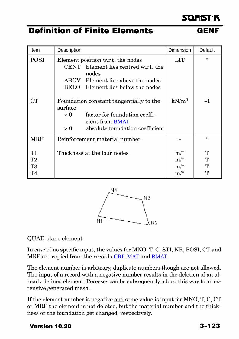
GENFDefinition of Finite Elements
3−123Version 10.20
Item DefaultDimensionDescription
POSI
CT
Element position w.r.t. the nodesCENT Element lies centred w.r.t. the
nodesABOV Element lies above the nodesBELO Element lies below the nodes
Foundation constant tangentially to thesurface
< 0 factor for foundation coeffi−cient from BMAT
> 0 absolute foundation coefficient
LIT
kN/m3
*
−1
MRF
T1T2T3T4
Reinforcement material number
Thickness at the four nodes
−
m/*m/*m/*m/*
*
TTTT
QUAD plane element
In case of no specific input, the values for MNO, T, C, STI, NR, POSI, CT andMRF are copied from the records GRP, MAT and BMAT.
The element number is arbitrary, duplicate numbers though are not allowed.The input of a record with a negative number results in the deletion of an al�ready defined element. Recesses can be subsequently added this way to an ex�tensive generated mesh.
If the element number is negative and some value is input for MNO, T, C, CTor MRF the element is not deleted, but the material number and the thick�ness or the foundation get changed, respectively.
GENF Definition of Finite Elements
Version 10.203−124
The element’s geometry is checked by the program for node numbering order,re−entrant corners and side ratios smaller than 1 : 5.
Entire rows of elements can be generated by a single record using DNO, ENOand NNO and, in combination to the generation capabilities of the input lan�guage, one can even generate multi−dimensional meshes.
If the record QUAD specifies a thickness T other than the one input by GRP,the gravity load and the isotropic stiffness are computed with this new thick�ness. In case of orthotropic thickness input by the record GRP, the orthotropicthicknesses of the GRP record are multiplied for computing the stiffness bythe factor T−QUAD / T−GRP.
The input of a negative value for C or CT represents a factor for the foundationcoefficient of the BMAT record, while a positive value determines an absolutefoundation coefficient for this element.
Several element actions can be selected through the value of STI. Additionof these values results in combined action. The preset values are:
SYST FRAM 2SYST GIRD 1SYST SPAC 7
Input of this value is meaningful, as a rule, only for three−dimensional sys�tems.
The orientation of the coordinate system is described in section 2.2.3. Bythree−dimensional systems the local x−axis can be oriented toward a particu�lar direction with respect to the global axes of coordinates; this can be of im�portance in the assessment of the results for the nodes. The following can bedefined as reference direction by NR:
XX,YY,ZZ for the positive directionsNEGX,NEGY,NEGZ for the negative directionsnodenumber of a node within local xz−plane
A negative value for NR defines an angle by which the default coordinate sys�tem is rotated aginst the local z−axis.
By POSI=BELO the elements are eccentrically below the nodes. This can beuseful in case of plates with girders for modelling the T−beam action by differ�ent element thicknesses. The input in such case is as easy as for a regular

GENFDefinition of Finite Elements
3−125Version 10.20
plate due to the constant altitude of the nodes lying at the upper edge of theplate. Because of the necessary axial force effects the analysis of eccentricplates can be done only with SYST SPAC by the program ASE.
The thicknesses T1 through T4 at the nodes are used for proportioning at thenodes only. Variable thicknesses at the nodes can not be input at the sametime with an orthotropy from GRP.

GENF Definition of Finite Elements
Version 10.203−126
See also: CUBE, MAT, GRP
3.48. BRIC − Three−dimensional
Solid Elements
ÄÄÄÄÄÄÄÄÄÄÄÄÄÄÄÄÄÄÄÄÄÄÄÄÄÄÄ
BRIC
Item Description Dimension Default
NO
N1N2N3N4N5N6N7N8
MNO
Element number
Number of node 1Number of node 2Number of node 3Number of node 4Number of node 5Number of node 6Number of node 7Number of node 8
Material number of the element
−
−−−−−−−−
−
!
!!!!!!!!
1
BRIC solid element
The element number is arbitrary, duplicate numbers though are not allowed.The input of a record with a negative element number causes the deletion ofan already defined element. Recesses can be subsequently added this way toa generated large surface mesh. If a value for MNO is input, the element isnot deleted, but the material number gets changed instead. The six sides ofthe element are checked geometrically by the program as QUAD−elements.
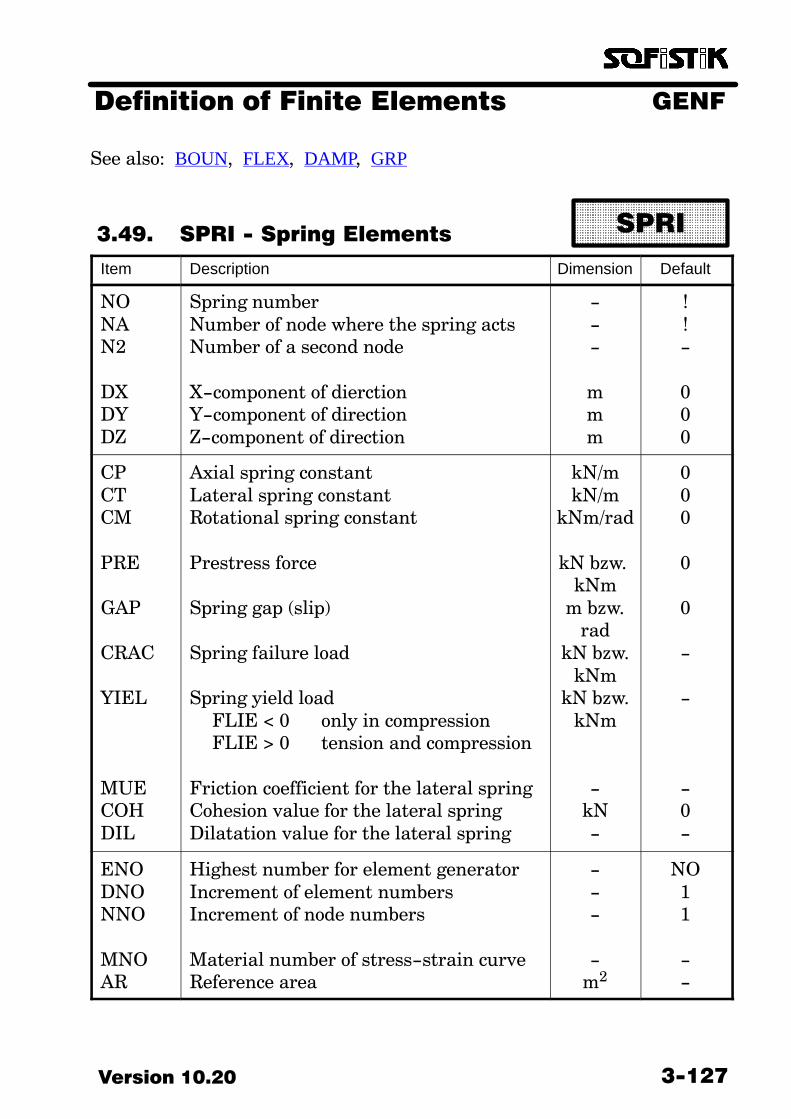
GENFDefinition of Finite Elements
3−127Version 10.20
See also: BOUN, FLEX, DAMP, GRP
3.49. SPRI − Spring Elements
ÄÄÄÄÄÄÄÄÄÄÄÄÄÄÄÄÄÄÄÄÄÄÄÄÄÄÄÄÄÄÄÄ
SPRI
Item Description Dimension Default
NONAN2
DXDYDZ
Spring numberNumber of node where the spring actsNumber of a second node
X−component of dierctionY−component of directionZ−component of direction
−−−
mmm
!!−
000
CPCTCM
PRE
GAP
CRAC
YIEL
MUECOHDIL
Axial spring constantLateral spring constantRotational spring constant
Prestress force
Spring gap (slip)
Spring failure load
Spring yield loadFLIE < 0 only in compressionFLIE > 0 tension and compression
Friction coefficient for the lateral springCohesion value for the lateral springDilatation value for the lateral spring
kN/mkN/m
kNm/rad
kN bzw. kNm
m bzw.rad
kN bzw.kNm
kN bzw.kNm
−kN−
000
0
0
−
−
−0−
ENODNONNO
MNOAR
Highest number for element generatorIncrement of element numbersIncrement of node numbers
Material number of stress−strain curveReference area
−−−
−m2
NO11
−−

GENF Definition of Finite Elements
Version 10.203−128
Spring element
Springs can be defined as support conditions or as coupling springs betweentwo nodes. The second node number must not be input in the first case.
The spring is defined by means of an axial direction (DX,DY,DZ) and twospring constants. The affected forces or deformations are then analysed intoa component in the axial direction and a remainder or lateral component per�pendicular to the axial one. The spring constants CP and CT are assigned tothe axial and the lateral direction, respectively. Two lateral springs perpen�dicular to each other with the same spring constants are likely to be assignedin this manner. Since the directions of these springs can be freely selected, onecan speak of an isotropic lateral spring stiffness. The total spring force hasthe following form :
P� ������PXPYPZ
����� ��
����DXDYDZ
�����PH�
����PTXPTYPTZ
����
PT� �� �PTX2 � PTY2 � PTZ2�1�2
The values of PH and PT affect the various combined nonlinear effects. In thegeneral three−dimensional case the lateral force can be input only in compo�nents or as an amount PT.
If one wants to prescribe different lateral spring stiffnesses, one should pre�scribe two or three separate axial springs. Since the input parameter CMusually does not agree neither in its direction of action nor regarding the non�linear effects with CP, it should not be input with a single element except forvery few cases. As a rule therefore, separate rotational springs (CP=CT=0.0)should be defined.

GENFDefinition of Finite Elements
3−129Version 10.20
The direction of coupling springs is derived from the difference of the twonodes (N2−NA). In cases of coinciding nodes or in cases of support springs, thedirection must be input explicitly. The method for choosing in this case thesigns of DX, DY and DZ, which are important for nonlinear computations(compression or tension?), is to imagine that the second node is offset from thefirst by this amount.
By defining a dilatation value, all lateral shear displacements will induce anaxial displacement DIL⋅u−t.
Nonlinear effects are controlled by PRE, CRAC, GAP, YIEL, MUE and COH:
Prestress:The spring exerts a force or a moment upon the node even in its initialposition. The failure and yield loads are appropriately modified by theamount of prestress. A prestress for the lateral spring is not defined.
Gap:The spring transmits forces along its axis only after its deformationhas exceeded the gap.
Failure load:Upon reaching the failure load the spring fails in both the axial andthe lateral direction. The failure load is always a tensile force or a posi�tive moment.
Yield load:Upon reaching the yield load, the deformation component of the springin its direction increases without a corresponding increase of the springforce.
Friction coefficient:If a friction and/or a cohesion coefficient are input, the lateral springcan not sustain forces greater than:
Friction_coeff. * Compressive_force + Cohesion
If the axial spring has significant tension or has failed (CRAC), the lat�eral force acts only if 0.0 has been input for both friction and cohesion.

GENF Definition of Finite Elements
Version 10.203−130
Spring force−displacement curves
The nonlinear effects can be taken into account only by a nonlinear analysis(STAR2/TALPA/ASE). The friction is an effect of the lateral spring, while allother effects act upon the axial spring (CP or CM). The program SEPPhandles springs as linear only without prestress.
Instead of these simple nonlinear effects you may assign a nonlinear materialworklaw to a spring element by the definition of MNO. You will then also needa influence area AR. The force of the spring is the product of the stress andthis area. For the stiffness or the strain you will need a length of the elementL:
L := (dx2+dy2+dz2)1/2CP := E−Modulus⋅AR/LCT := G−Modulus⋅AR/LP := CP⋅us := P/ARe := u/L
This value A/L will also be used indenpendent of MNO by HYDRA for the con�struction of equivalent thermal or seepage conductivities.
For a torsional spring however AR will be equivalent to the torsional inertiain m4:
CM := G−Modulus⋅AR/LM := G−Modulus⋅AR⋅φ/Lσ := M/AR/L
The stress−strain curve is established for a fictive stress in dependance fromthe torsional strain φ/L.

GENFDefinition of Finite Elements
3−131Version 10.20
The definition of a negative value for AR will select an inverse treatement ofthe nonlinear effects. The force in the axial direction will not become greaterthan COH+MUE⋅of the vectorlength of the combined transvers force, whichwill not become greater than YIEL. This is usefull for the description of an�chors and piles in soil mechanics.
With an input of MNO CP and Ct are calculated automatically. If one or bothvalues, e.g. at an input of CM, are not used, the value 0 is entered for CPand/or CT.
ATTENTION: The above effects and the dilatation are new and will becomeimplemented in the various modules step after step. Please read the relevanthtm−files.
Special instructions
More complicated force−displacement curves can be generated by combiningseveral nonlinear springs in parallel or in series. A change of the directioncomponent signs can be very helpful in these combinations. These signs havean effect on the sign of the spring force.
Negative spring constants can be used for the modelling of suspended pendu�lum towers according to 2nd order theory or for similar effects. Attentionshould be given in this case to the correct consideration of the load safety fac�tor.
Additional springs with small spring constants can possibly make the conver�gence easier or even enable it in the first place during nonlinear computa�tions.
The prestress is the same for all loadings, therefore it can not be used, in gen�eral, for load superpositioning by the program MAXIMA.
The element generator (ENO, DNO and NNO) generates springs along thespecified nodes, which are defined by the geometry of their distances from oneanother. All spring constants and material properties must be input in thiscase per unit length. The program computes automatically the resulting dis�cretised spring stiffnesses from the varying distances between nodes.
The input of a record with a negative spring number results in the deletionof an already defined element.
Support displacements or rotations can be described for the FE−programsSEPP, TALPA and ASE by a spring of stiffness 1E20 and a loading equal to

GENF Definition of Finite Elements
Version 10.203−132
displacement times 1E20. This technique avoids the rebuilding of the equa�tion system for each particular loadcase.

GENFDefinition of Finite Elements
3−133Version 10.20
See also: SPRI, FLEX, GRP, NODE
3.50. BOUN − Distributed Elastic
Support
ÄÄÄÄÄÄÄÄÄÄÄÄÄÄÄÄÄÄÄÄÄÄÄÄÄÄÄÄÄÄÄÄ
BOUN
Item Description Dimension Default
FROMTOINC
TYPE
CACE
Starting node or element numberEnd node numberIncrementAll nodes from FROM to TO in in�crements of INC are elastically sup�ported.
Direction of supportCX Support in global X−dirctionCY Support in global Y−directionCZ Support in global Z−directionCN Support in longitudinal direc−
tion (axial force)CT Support in both transverse
directions (shear force)DX Fixing about global X−
directionDY Fixing about global Y−
directionDZ Fixing about global Z−
directionDN Fixing about longitudinal
directionDT Fixing about both transverse
directions
Spring constants at the beginningSpring constants at the end
−−−
LIT
kN/m2
or kN
!FROM
!
!
!CA
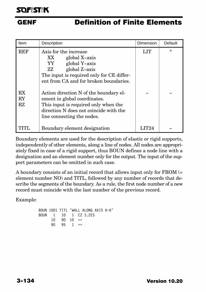
GENF Definition of Finite Elements
Version 10.203−134
Item DefaultDimensionDescription
REF
RXRYRZ
TITL
Axis for the increaseXX global X−axisYY global Y−axisZZ global Z−axis
The input is required only for CE differ�ent from CA and for broken boundaries.
Action direction N of the boundary el�ement in global coordinates.This input is required only when thedirection N does not coincide with theline connecting the nodes.
Boundary element designation
LIT
−
LIT24
*
−
−
Boundary elements are used for the description of elastic or rigid supports,independently of other elements, along a line of nodes. All nodes are appropri�ately fixed in case of a rigid support, thus BOUN defines a node line with adesignation and an element number only for the output. The input of the sup�port parameters can be omitted in such case.
A boundary consists of an initial record that allows input only for FROM (=element number NO) and TITL, followed by any number of records that de�scribe the segments of the boundary. As a rule, the first node number of a newrecord must coincide with the last number of the previous record.
Example:
BOUN 1001 TITL ’WALL ALONG AXIS K−K’ BOUN 1 10 1 CZ 3.2E5 10 90 10 == 90 95 1 ==
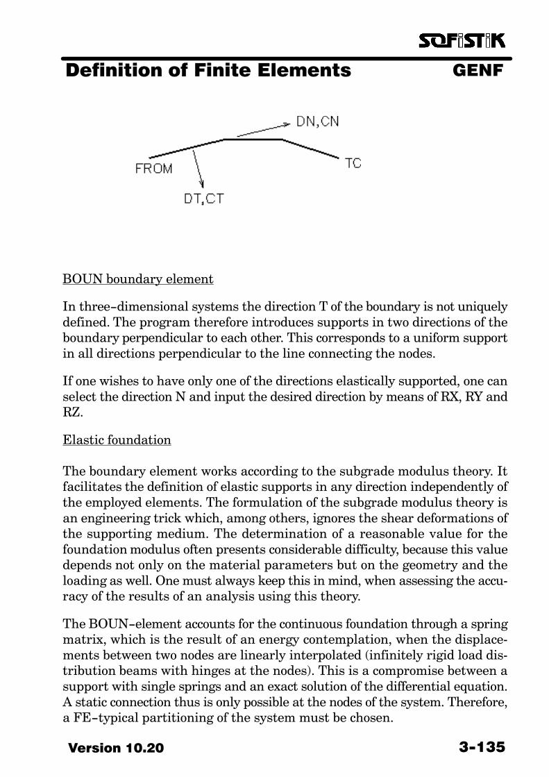
GENFDefinition of Finite Elements
3−135Version 10.20
BOUN boundary element
In three−dimensional systems the direction T of the boundary is not uniquelydefined. The program therefore introduces supports in two directions of theboundary perpendicular to each other. This corresponds to a uniform supportin all directions perpendicular to the line connecting the nodes.
If one wishes to have only one of the directions elastically supported, one canselect the direction N and input the desired direction by means of RX, RY andRZ.
Elastic foundation
The boundary element works according to the subgrade modulus theory. Itfacilitates the definition of elastic supports in any direction independently ofthe employed elements. The formulation of the subgrade modulus theory isan engineering trick which, among others, ignores the shear deformations ofthe supporting medium. The determination of a reasonable value for thefoundation modulus often presents considerable difficulty, because this valuedepends not only on the material parameters but on the geometry and theloading as well. One must always keep this in mind, when assessing the accu�racy of the results of an analysis using this theory.
The BOUN−element accounts for the continuous foundation through a springmatrix, which is the result of an energy contemplation, when the displace�ments between two nodes are linearly interpolated (infinitely rigid load dis�tribution beams with hinges at the nodes). This is a compromise between asupport with single springs and an exact solution of the differential equation.A static connection thus is only possible at the nodes of the system. Therefore,a FE−typical partitioning of the system must be chosen.
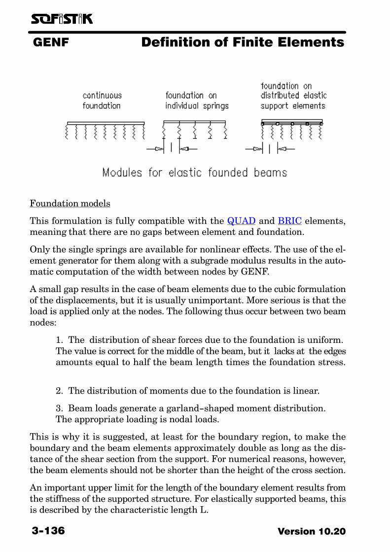
GENF Definition of Finite Elements
Version 10.203−136
Foundation models
This formulation is fully compatible with the QUAD and BRIC elements,meaning that there are no gaps between element and foundation.
Only the single springs are available for nonlinear effects. The use of the el�ement generator for them along with a subgrade modulus results in the auto�matic computation of the width between nodes by GENF.
A small gap results in the case of beam elements due to the cubic formulationof the displacements, but it is usually unimportant. More serious is that theload is applied only at the nodes. The following thus occur between two beamnodes:
1. The distribution of shear forces due to the foundation is uniform.The value is correct for the middle of the beam, but it lacks at the edgesamounts equal to half the beam length times the foundation stress.
2. The distribution of moments due to the foundation is linear.
3. Beam loads generate a garland−shaped moment distribution.The appropriate loading is nodal loads.
This is why it is suggested, at least for the boundary region, to make theboundary and the beam elements approximately double as long as the dis�tance of the shear section from the support. For numerical reasons, however,the beam elements should not be shorter than the height of the cross section.
An important upper limit for the length of the boundary element results fromthe stiffness of the supported structure. For elastically supported beams, thisis described by the characteristic length L.

GENFDefinition of Finite Elements
3−137Version 10.20
L� �� �4 � EIc � b
�4�The solution for the displacement under concentrated loads is a wave, whichalways has a zero crossing at distance L. For the boundary element to be ableto approximate that, its segments must be smaller than one quarter of thatlength.
When this is not the case, the boundary element searches to represent thatdistribution through a wild oscillation. The results are severely disturbedin this manner. If the structure’s stiffness is zero, the characteristic lengthis zero as well, and the boundary element can not be used for concentratedloads at all.
Comparative analyses have shown, that an elastically supported beam is sig�nificantly better approximated by boundary elements with continuousfoundation than by single springs.
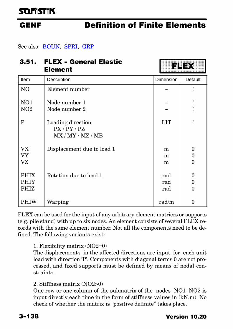
GENF Definition of Finite Elements
Version 10.203−138
See also: BOUN, SPRI, GRP
3.51. FLEX − General Elastic
Element
ÄÄÄÄÄÄÄÄÄÄÄÄÄÄÄÄÄÄÄÄÄÄÄÄÄÄÄÄÄÄÄÄÄÄÄÄ
FLEX
Item Description Dimension Default
NO
NO1NO2
P
VXVYVZ
PHIXPHIYPHIZ
PHIW
Element number
Node number 1Node number 2
Loading directionPX / PY / PZMX / MY / MZ / MB
Displacement due to load 1
Rotation due to load 1
Warping
−
−−
LIT
mmm
radradrad
rad/m
!
!!
!
000
000
0
FLEX can be used for the input of any arbitrary element matrices or supports(e.g. pile stand) with up to six nodes. An element consists of several FLEX re�cords with the same element number. Not all the components need to be de�fined. The following variants exist:
1. Flexibility matrix (NO2=0)The displacements in the affected directions are input for each unitload with direction ’P’. Components with diagonal terms 0 are not pro�cessed, and fixed supports must be defined by means of nodal con�straints.
2. Stiffness matrix (NO2>0)One row or one column of the submatrix of the nodes NO1−NO2 isinput directly each time in the form of stiffness values in (kN,m). Nocheck of whether the matrix is "positive definite" takes place.

GENFDefinition of Finite Elements
3−139Version 10.20
3. Identifier for substructuring (NO2 = "SUBS")When this literal is input, node NO1 is identified as the main node ofthe substructure. The inverse values of the stiffness can then be pre�scribed by the displacement values (see HASE). Only one record pernode is allowed in this case.

GENF Definition of Finite Elements
Version 10.203−140
See also: SPRI, MASS
3.52. DAMP − Damping Elements
ÄÄÄÄÄÄÄÄÄÄÄÄÄÄÄÄÄÄÄÄÄÄÄÄÄÄÄÄÄÄÄÄÄÄÄÄ
DAMP
Item Description Dimension Default
NO
NANE
DDTDM
Element number
Start nodeEnd node
Damping in axial directionDamping in lateral directionDamping moment about the axis
−
−−
kNsec/mkNsec/m
kNsec
1
10
0.0.0.
The direction of the damping element is defined by the nodes NA and NE. Thedamping coefficient DT acts perpendicularly to it. The damping element isused in dynamic analysis only.
Damping element
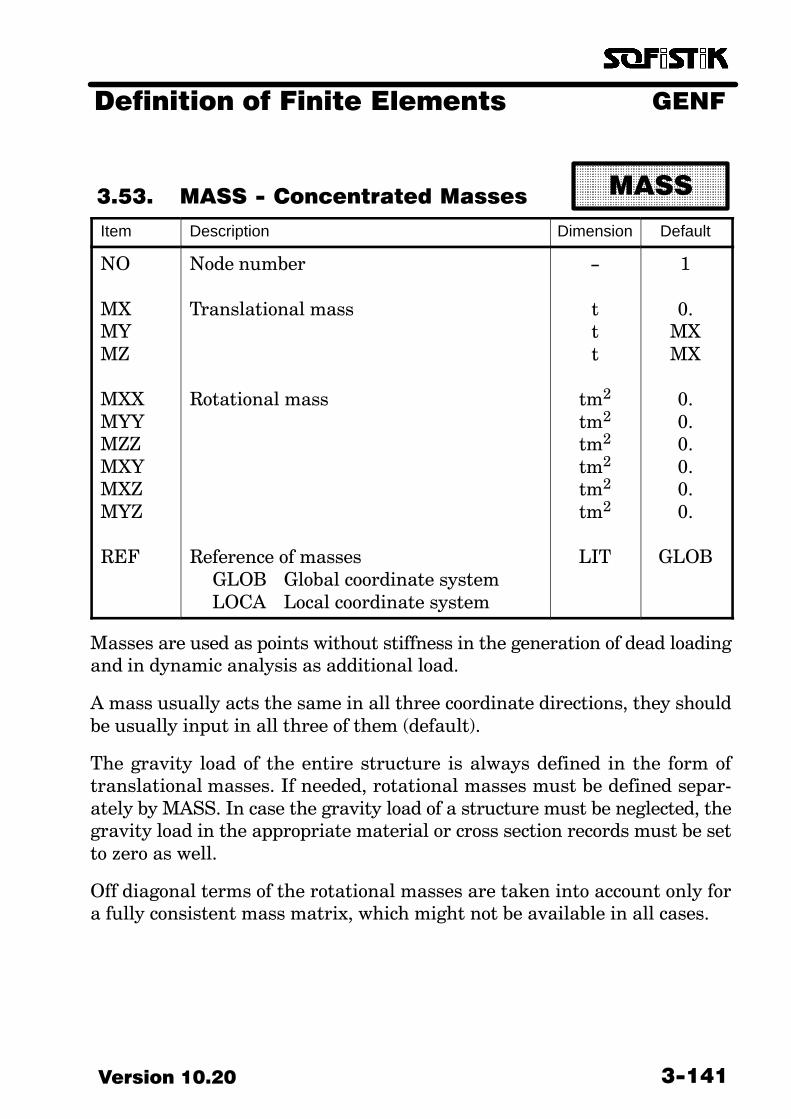
GENFDefinition of Finite Elements
3−141Version 10.20
3.53. MASS − Concentrated Masses
ÄÄÄÄÄÄÄÄÄÄÄÄÄÄÄÄÄÄÄÄÄÄÄÄÄÄÄÄÄÄÄÄ
MASS
Item Description Dimension Default
NO
MXMYMZ
MXXMYYMZZMXYMXZMYZ
REF
Node number
Translational mass
Rotational mass
Reference of massesGLOB Global coordinate systemLOCA Local coordinate system
−
ttt
tm2
tm2
tm2
tm2
tm2
tm2
LIT
1
0.MXMX
0.0.0.0.0.0.
GLOB
Masses are used as points without stiffness in the generation of dead loadingand in dynamic analysis as additional load.
A mass usually acts the same in all three coordinate directions, they shouldbe usually input in all three of them (default).
The gravity load of the entire structure is always defined in the form oftranslational masses. If needed, rotational masses must be defined separ�ately by MASS. In case the gravity load of a structure must be neglected, thegravity load in the appropriate material or cross section records must be setto zero as well.
Off diagonal terms of the rotational masses are taken into account only fora fully consistent mass matrix, which might not be available in all cases.

GENF Definition of Finite Elements
Version 10.203−142
This page intentionally left blank

GENFDefinition of Finite Elements
4−1Version 10.20
4 Output Description
In case of error−free input, all input records are output as well. This can beprevented by setting ECHO NO; by contrast, setting ECHO PRIN results infull output regardless of whether the input is correct or not.
By use of the options of the ECHO record, one can obtain a selective output,e.g., ECHO NODE NO means that node data should not be printed.
The results of the profile optimisation of the stiffness matrix are output onthe screen as well as in the output file. The bandwidth and the profile are out�put here without consideration of the degree of freedom per node.
4.1. Nodal Values
With ECHO NODE YES all nodal coordinates and the relevant supports (nodecelebration attributes) and the kinematic constraints are spent.
Meaning nodal coordinates and supports in the list:
Number Node numberX X−coordinate in mY Y−coordinate in mZ Z−coordinate in mSupport Conditions Support conditions of a node (Explanation of
the short cut see record NODE)MIN minimal nodal valueMAX maximal nodal value
According to the input the list of the kinematic constraints is made addition�ally. With input of couplings at NODE and/or of intermediate nodes with INTEthe list results followingly:
Node Node numberLV Level of coupling with recursive definitiontype Coupling condition (Explanation of the short
cut see record NODE) or with definition modelintermediate node of the interpolationINTtyp (Explanation of typ see record INTE)
reference Reference node

GENF Definition of Finite Elements
Version 10.204−2
dx,dy,dz Direction of the couplings or effective dis−tances between the nodes
df general factor, indicates where the inter−mediate node (INTE) lies between thereference nodes
With input of the kinematic dependences with the record KINE following listis made:
ND Dependent degree of freedom indicated withnode number/local degree of freedom
LV Level of coupling with recursive definitionND1 Reference degree of freedom 1 indicated with
node number/local degree of freedom withX,Y,Z for the displacements an XX,YY,ZZ forthe rotations
FD1 Factor for reference degree of freedom 1 . . .ND6FD6
4.2. Material Values
In the normal case (ECHO MAT YES) a list from the tables of the material va�lues is following:
General Material ValuesNo Material numberYoung−module Elastic modulusPoisson−Ratio Poisson’s ratioShear−module Shear modulusCompress.module Bulk modulusWeight Specific weightWeight buoyancy Specific weight under buoyancy, only for soil
mechanicsTemperat. coeff. Thermal expansion coefficientY−Modulus E−y Anisotropic elastic modulusPoisson R. m−yz Anisotropic Poisson’s ratioAngle Rotation Meridian angle of anisotropy

GENFDefinition of Finite Elements
4−3Version 10.20
Angle Precission Descent angle of anisotropySafetyfactor Material safety factorcalc strength fy Calculation strengthult. strength ft Final strength
Non−linear Material Values
With input of a non−linear material (NMAT) law the parameters of thematerial law are spent to the general material values additionally(Parameter discription in the manual TALPA).
Bedding AttributesNo Material numberCs Elastic constant normal to surfaceCt Elastic constant tangential to surfacepr Maximum tensile stress of interfacepy Maximum stress of interfacetan Friction coefficient of interfacec Cohesion of the interfacew Equivalent mass distribution
C O N C R E T E M A T E R I A LStrength fc Design value of concrete strengthNominal strength Cube strength or cylinder compressive
strengthTens.Str. fctm average tensile strengthTens.Str. fctk Fractile of the tensile strengthCompr.fail.ener. Fracture energy for compression failureTens.fail.energ. Fracture energy for tensile failureFriction crack Friction in the crack
S T E E L M A T E R I A LYield stress fy Yield stregthTensile str. ft Tensile strengthPlastic strain Failure strainRelaxation .55ft Coefficient of relaxation (0.55 ßz)Relaxation .70ft Coefficient of relaxation (0.70 ßz)nat. bond coeff. Bond coefficient by DIN 4227 Table 8.1EC2 bondcoeff K1 Bond coefficient per EC2 / Vol. 400Hardening module Hardening module
GENF Definition of Finite Elements
Version 10.204−4
T I M B E R M A T E R I A LBendingstr fm Bending strengthTensionstr ft,0 Tensile strength parallel to the fibreTensionstr ft,90 Tensile strength normal to the fibreCompress. fc,0 Compressive strength parallel to the fibreCompress. fc,90 Compressive sterength normal to the fibreShearstr. fv Shear strength at center (shear force)Shearstr. fv,T Shear strength at edge (torsion)
The entered stress−strain curves are not spent. An output of the stress−strain curves occurs only with input in the programm AQUA. Graphic repre�sentations of the stress−strain curves are possible with AQUP.
A layerd material was entered with the record MLAY, so the general materialvalues of this material are determined and spent. The layer are entered addi�tionally:
Layer thickness Layer thickness in mMaterial No. Material number and material specification
of the layer
Up to ten shifts are spent according to the input.
4.3. System Statistics
A list of several cross sectional types according to input of BEAM, TRUS, CABLor plane elements according to input QUAD is made with ECHO SYST YES.
Meaning summary of the several cross sectional types in the list:
No. Number of the cross sectionTotal Length Total Length in mTotal Weight Total Weigth in tmax. Length Maximum Length in mTitle Title
Meaning summary of used plane elements in system in the list:
Grp Number of the groupTotal Area Total Area in m2Total Weight Total Weight in tmax. area Maximum area of an element in m2Total Volume Total Volume in m3Material No. Material number
GENFDefinition of Finite Elements
4−5Version 10.20
4.4. Cross−sectional Overview
With ECHO SECT YES a overview of the cross−sectional values is spent. Inthat means:
CROSS SECTIONS − STATIC PROPERTIES
No Number of the cross sectionMNo Material number of the cross sectionMNs Material number of the reinforcementA Cross−sectional area in m2
It Torsional moment of inertia in m4
Ay,Az,Ayz Shear areas in m2
Iy,Iz,Iyz Moments of inertia y,z,yz in m4
ys,zs Coordinates of centre of gravity in my,z−sc Coordinates of shear centre in mmodules Elastic and shear modulus in kN/m2
gam Specific weight in kN/m3
Provided that a cross−section designation was defines, this is appended so be�hind every cross section.
An output of the supplementary cross−sectional values (moments of resis�tance, fully plastic internal forces and moments, reinforcement etc.) is poss�ible only after input with the program AQUA.
4.5. Group Qualities
An output of the group qualities occurs with ECHO GROU YES. In the list ofthe group qualities means:
No Number of the groupMNo Material numberMrf Material number of the reinforcementAnsatz Element formulationPosi Position of the elements to the nodesDirection x−axis Direction of the local x−axisThick Thickness of the elements in mOrthotropic thickn. Orthotropic thicknesses of the elements in m DX,DY,DXY,DD (Output occurs only in case od differences to
the thickness.)

GENF Definition of Finite Elements
Version 10.204−6
4.6. Plane Elements (2−D, QUAD)
An output of the group qualities occurs with ECHO QUAD YES. In the list ofthe group qualities means:
Grp Number of the groupNumber Element numberNodeno Node numbers of the corner nodesNodenoNodenoNodenoMNo Material numbert Thickness of the element in mC Elastic foundation in kN/m3Orthotropic thickn. Orthotropic thicknesses of the element in m TX,TY,TXY,TD (Output occurs only in case od differences to
the thickness.)Variable thickness Variable thicknesses of the elements in m t1 − t4 (An output occurs only with different thick−
nesses in the nodes.)
Footnotes to the several output values are explained in the ERG−file.
4.7. Three−dimensional Solid Elements (3−D, BRIC)
The three−dimensional solid elements are spent after input of ECHO BRICYES in following list:
Grp Number of the groupNumber Element numberNodeno Number of the node 1Nodeno Number of the node 2Nodeno Number of the node 3Nodeno Number of the node 4Nodeno Number of the node 5Nodeno Number of the node 6Nodeno Number of the node 7Nodeno Number of the node 8MNo Material number of the element

GENFDefinition of Finite Elements
4−7Version 10.20
4.8. Boundary Elements
With the record ECHO BOUN YES lists of the boundary elements (BOUN), theelement matrixes and supports (FLEX), the damping elements (DAMP) andthe single masses (MASS) are spent.
After the input of the record BOUN − Distributed Elastic Support followinglist appears:
from Starting node or element numberto End node numberinc Incrementtype Direction of supportref Axis for the increaseCA/CB Spring constants at the beginning/endTitle/Direction Boundary element designation/directionTotal Length Total Length in m
After input of the record FLEX − General Elastic Support an element matrixfollows in the output listing:
Number Number of the elementNodeno Node number, negatively at Substructering
F−xx,F−yy,F−zz, Values of the flexibility matrixFR−xx,FR−yy,FR−zz,FR−ww
S−xx,S−yy,S−zz, Values of the stiffness matrixSR−xx,SR−yy,SR−zz
At the substructure−technique the shift−values of the stiffness are spent.
If damping elements were entered with the record DAMP, a list of the damp�ing elements is spent:
Grp Number of the groupNumber Element numberNodeno Star nodeNodeno End nodedX,dY,dZ Indication of direction of the damping
elementDP Damping in axial direction in kNsec/m

GENF Definition of Finite Elements
Version 10.204−8
DT Damping in lateral direction in kNsec/mDM Damping moment about the axis in kNsec
If an input of single masses with the record MASS occurs, these are spent soas follows:
Nodeno Node numberGroup Number of the groupM−X,M−Y,M−Z Translational masses in tM−XX,M−YY,M−ZZ Rotational masses in tm2
4.9. Geometric Definitions (Bedding Profiles)
Bedding profiles with the records BORE, BBAX, BBLA were entered in con�nection with the pile elements or for analysis of settlement, the output of thevalues with ECHO GEOD YES in a list of the structural axis / bedding axisoccurs so. In that means:
Line Line number of the structural/bedding axiss Starting and/or ending depthx,y,z Coordinates of the well site in mL Length in mK0−a,K1−a,K2−a, Constants of the foundation profile K3−aM0 Mantle friction in kN/mC0 Cohesion coefficient in kN/mTANR Soil/pile friction angle in degreesTAND Dilatation angle in degrees (SOFIMESH
only)KSIG Lateral pressure value (SOFIMESH only)K0−t,K1−t,K2−t, Constants of foundation profile in tangential K3−t direction (lateral) in kN/m2
P0,P1,P2,P3 Factors for circumferential variationPmax Maximum foundation value at starting and
ending depth in kN/m
4.10. Bending Beams and Piles
An output of the bending beams and piles occurs with ECHO BEAM YES.
For the entered bending beams and piles (BEAM) following list appears:

GENFDefinition of Finite Elements
4−9Version 10.20
Grp Number of the groupNumber Beam numberNodeno Number of the start and/or end beam nodex Distance of the beam beginning in mNoS Cross section numberRef Reference axis (at genrated pile elements
geometry or bedding number)hinges Hinge combination (Explanation of the short
cut see records HING and BEAM)direction local Direction data of local y−axisy−axis
After definition of beam sections with the records ADEF and BDIV or of beamsections with the record BSEC or of supporting sections with the record SUPPadditional to the list of bending beams the type, the direction and the placeof the defined beam sections are spent (Explanations see BEAM, ADEF, BDIV,BSEC and SUPP).
4.11. Truss−bar Elements
A list of truss−bar elements is made with ECHO TRUS YES. In that means:
Grp Number of the groupNumber Number of the truss−barNodeno Start nodeNodeno End nodesection Cross section numberL Length in mN−p Prestress force in kN
4.12. Cable Elements
With ECHO CABL YES a following list of cable elements is spent:
Grp Number of the groupNumber Number of the cable elementNodeno Start nodeNodeno End nodesection Cross section numberL Length in mN−p Prestress force in kN

GENF Definition of Finite Elements
Version 10.204−10
4.13. Springs
Spring values are spent with ECHO SPRI YES in two lists. The general springvalues appear in the list SPRING ELEMENTS:
Grp Number of the groupNumber Spring numberNodeno Number of node upon which the spring actsNodeno Number of a second nodedX,dY,dZ Components of direction X,Y,ZCP Axial spring constant in kN/mCT Lateral spring constant in kN/mCM Rotational spring constant in kNm/radN−p Prestress force in kN and/or kNm
The list NONLINEAR EFFECTS is made only by input of one of these values:
Grp Number of the groupNumber Spring numberPrestress Prestress force in kN and/or kNmGap Spring gap (slip) in mmT−Cutoff Spring failure load in kN and/or kNmYielding Sprinf yield load in kN and/or kNmFriction Friction coefficient for the lateral springCohesion Cohesion value for the lateral spring in kN
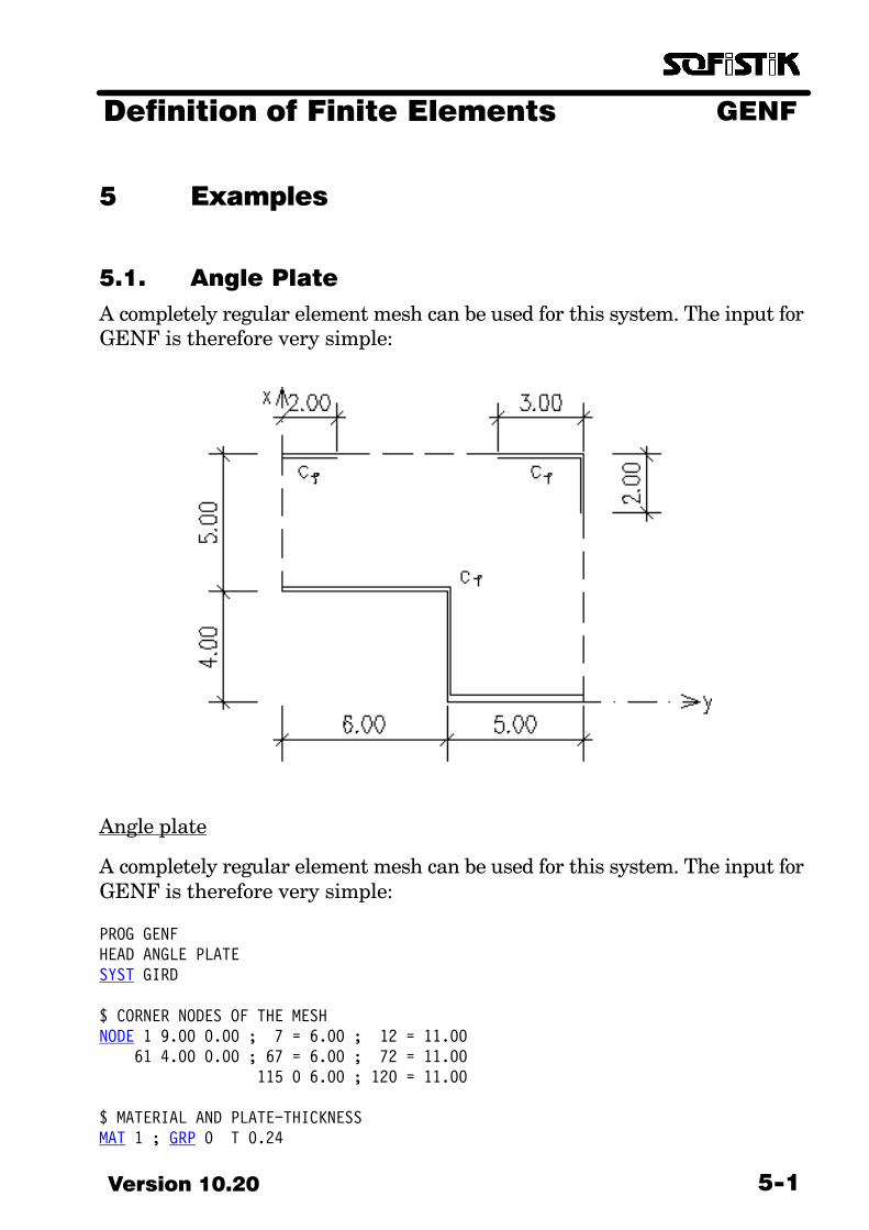
GENFDefinition of Finite Elements
5−1Version 10.20
5 Examples
5.1. Angle Plate
A completely regular element mesh can be used for this system. The input forGENF is therefore very simple:
Angle plate
A completely regular element mesh can be used for this system. The input forGENF is therefore very simple:
PROG GENFHEAD ANGLE PLATESYST GIRD
$ CORNER NODES OF THE MESHNODE 1 9.00 0.00 ; 7 = 6.00 ; 12 = 11.00 61 4.00 0.00 ; 67 = 6.00 ; 72 = 11.00 115 0 6.00 ; 120 = 11.00
$ MATERIAL AND PLATE−THICKNESSMAT 1 ; GRP 0 T 0.24
GENF Definition of Finite Elements
Version 10.205−2
$ GENERATION OF THE MESHMESH 61 67 7 1 6 5 1 ; 67 72 12 7 5 5 1 ; 115 120 72 67 5 4 1
$ SUPPLEMENT OF THE BOUNDARY CONDITIONSNODE (61 66 1) − − PZMX ; 67 − − F ; (79 115 12) − − PZMY ( 1 3 1) − − PZMX ; (9 11 1) == ; 12 − − F (24 36 12) − − PZMY ; 115 − − F ; (116 120 1) − − PZMX
$ FIXING ACTION OF THE BOUNDARIES$ ROTATIONAL FOUNDATION CONSTANT D = 3EI/L= 3*3E7*0.24**3/12/3BOUN 1 TITL ’INTERNAL WALL’; BOUN 1 3 1 DN 34560 9 12 1 == ; 12 36 12 ==BOUN 2 TITL ’EXTERNAL WALL’; BOUN 61 67 1 == 67 115 12 == ; 115 120 1 ==END
The input for the program GRAF is as follows:
PROG GRAFHEAD GRAPHICSVIEW STAN 0 0 −1 NEGXCOLO C5 6000SCHH H3 0.4STRU 1 1 MARK 0END

GENFDefinition of Finite Elements
5−3Version 10.20
The following system results:
Mesh partitioning
5.2. Pointwise Supported Ceiling Plate
A real system from the design practice is presented in the following example.The statical system and the relevant assumptions are shown in the figure(refer also to SEPP−Manual Example 5.6.)
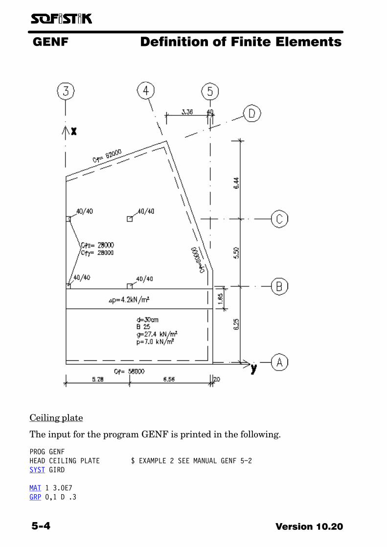
GENF Definition of Finite Elements
Version 10.205−4
Ceiling plate
The input for the program GENF is printed in the following.
PROG GENFHEAD CEILING PLATE $ EXAMPLE 2 SEE MANUAL GENF 5−2SYST GIRD
MAT 1 3.0E7GRP 0,1 D .3
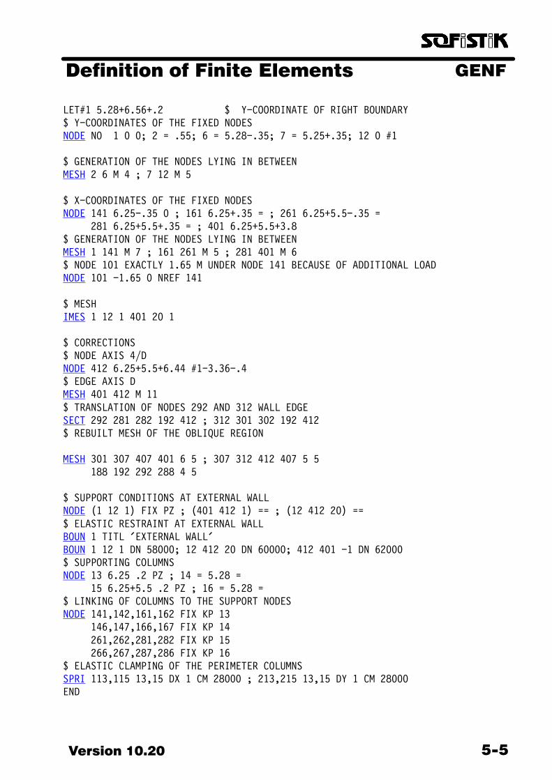
GENFDefinition of Finite Elements
5−5Version 10.20
LET#1 5.28+6.56+.2 $ Y−COORDINATE OF RIGHT BOUNDARY$ Y−COORDINATES OF THE FIXED NODESNODE NO 1 0 0; 2 = .55; 6 = 5.28−.35; 7 = 5.25+.35; 12 0 #1
$ GENERATION OF THE NODES LYING IN BETWEENMESH 2 6 M 4 ; 7 12 M 5
$ X−COORDINATES OF THE FIXED NODESNODE 141 6.25−.35 0 ; 161 6.25+.35 = ; 261 6.25+5.5−.35 = 281 6.25+5.5+.35 = ; 401 6.25+5.5+3.8$ GENERATION OF THE NODES LYING IN BETWEENMESH 1 141 M 7 ; 161 261 M 5 ; 281 401 M 6$ NODE 101 EXACTLY 1.65 M UNDER NODE 141 BECAUSE OF ADDITIONAL LOADNODE 101 −1.65 0 NREF 141
$ MESHIMES 1 12 1 401 20 1
$ CORRECTIONS$ NODE AXIS 4/DNODE 412 6.25+5.5+6.44 #1−3.36−.4$ EDGE AXIS DMESH 401 412 M 11$ TRANSLATION OF NODES 292 AND 312 WALL EDGESECT 292 281 282 192 412 ; 312 301 302 192 412$ REBUILT MESH OF THE OBLIQUE REGION
MESH 301 307 407 401 6 5 ; 307 312 412 407 5 5 188 192 292 288 4 5
$ SUPPORT CONDITIONS AT EXTERNAL WALLNODE (1 12 1) FIX PZ ; (401 412 1) == ; (12 412 20) ==$ ELASTIC RESTRAINT AT EXTERNAL WALLBOUN 1 TITL ’EXTERNAL WALL’BOUN 1 12 1 DN 58000; 12 412 20 DN 60000; 412 401 −1 DN 62000$ SUPPORTING COLUMNSNODE 13 6.25 .2 PZ ; 14 = 5.28 = 15 6.25+5.5 .2 PZ ; 16 = 5.28 =$ LINKING OF COLUMNS TO THE SUPPORT NODESNODE 141,142,161,162 FIX KP 13 146,147,166,167 FIX KP 14 261,262,281,282 FIX KP 15 266,267,287,286 FIX KP 16$ ELASTIC CLAMPING OF THE PERIMETER COLUMNSSPRI 113,115 13,15 DX 1 CM 28000 ; 213,215 13,15 DY 1 CM 28000END
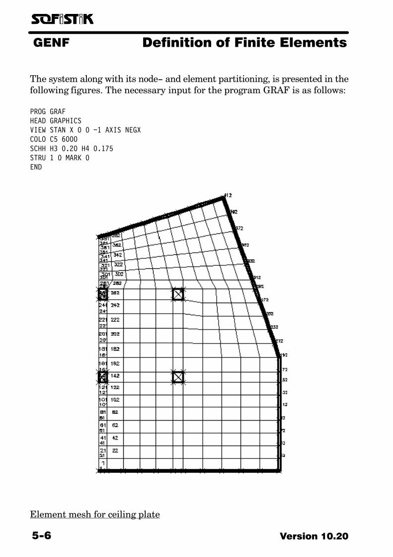
GENF Definition of Finite Elements
Version 10.205−6
The system along with its node− and element partitioning, is presented in thefollowing figures. The necessary input for the program GRAF is as follows:
PROG GRAFHEAD GRAPHICSVIEW STAN X 0 0 −1 AXIS NEGXCOLO C5 6000SCHH H3 0.20 H4 0.175STRU 1 0 MARK 0END
Element mesh for ceiling plate

GENFDefinition of Finite Elements
5−7Version 10.20
5.3. Gridwork
Gridworks lie in the X−Y plane and they are stressed perpendicularly to theirplane. The Z−axis in this case points downwards. The resulting basic forcesare Vz, Mt and My (corresponding to the cross sectional parameters Az, It andIy).
Gridwork
A 2−span gridwork with 3 main girders serves as example. The input toGENF reads: (refer also to STAR2−Manual Example 5.3.)
PROG GENFHEAD GRID FRAMEWORKSYST GIRDNODE 1 0 7 ; 7 24 7 ; 21 0 0 ; 27 24 0MESH 1 7 27 21 6 2$ SUPPORTINGSNODE (1 21 10) − − PZ ; (4 24 10) − − PZ ; (7 27 10) − − PZCONC 1 C 25SVAL 1 1 1 − − .024279 .030375SVAL 2 1 1 − − .002794 .003125BEAM ( 1 6 1) ( 1 1) ( 2 1) 1 − − 4BEAM (11 16 1) (11 1) (12 1) 1 − − 4BEAM (21 26 1) (21 1) (22 1) 1 − − 4BEAM (31 37 1) ( 1 1) (11 1) 2 − − 4BEAM (41 47 1) (11 1) (21 1) 2 − − 4END
The GENF−output is as follows:

GENF Definition of Finite Elements
Version 10.205−8
M A X I M U M N O D A L P A R A M E T E R S max−No Xmin/Xmax Ymin/Ymax Zmin/Zmax 27 .000 .000 .000 24.000 7.000 .000
NODAL COORDINATES AND SUPPORTS Number X (m) Y (m) Z (m) Support Conditions 1 .000 7.000 .000 PX PY PZ MZ MB 2 4.000 7.000 .000 PX PY MZ MB 3 8.000 7.000 .000 PX PY MZ MB 4 12.000 7.000 .000 PX PY PZ MZ MB 5 16.000 7.000 .000 PX PY MZ MB 6 20.000 7.000 .000 PX PY MZ MB 7 24.000 7.000 .000 PX PY PZ MZ MB 11 .000 3.500 .000 PX PY PZ MZ MB 12 4.000 3.500 .000 PX PY MZ MB ... ...
M A T E R I A L S
No. 1 C 25 (Eurocode EC2) −−−−−−−−−−−−−−−−−−−−−−−−−−−−−−−−−−−−−−−−−−−−−−−−−−−−−−−−−−−−−−−−−−−−−−−− Young−module 30472 [MPa] Safetyfactor 1.50 [−] Poisson−Ratio .20 [−] Strength fc 21.25 [MPa] Shear−module 12696 [MPa] Nominal Strength 25.00 [MPa] Compress.module 16929 [MPa] Tens.Str. fctm 2.56 [MPa] Weight 25.0 [kN/m3] Tens.Str. fctk 1.80 [MPa] Weight buoyancy .0 [kN/m3] Tens.Str. fctm 3.33 [MPa] Temperat. coeff. 1.00E−05 [−] Compr.fail.ener. 20.00 [kN/m] Tens.fail.energ. .05 [kN/m] Friction crack .20 [−]
C R O S S − S E C T I O N S S T A T I C P R O P E R T I E S
No MNo A[m2] Ay/Az/Ayz Iy/Iz/Iyz ys/zs y/z−sc modules gam MNs It[m4] [m2] [m4] [m] [m] [MPa] [kN/m3] 1 1 1.0000E+00 3.038E−02 .000 .000 30472 25.0 2.428E−02 3.038E−02 .000 .000 12696 2 1 1.0000E+00 3.125E−03 .000 .000 30472 25.0 2.794E−03 3.125E−03 .000 .000 12696
B E A M E L E M E N T S beam− node− x NP NCO hinges direction of No. No. (M) local y−axis 1 1 .000 1 .00 1.00 .00 1.000 1 2.000 1

GENFDefinition of Finite Elements
5−9Version 10.20
3.000 1 2 4.000 1 2 2 .000 1 .00 1.00 .00 1.000 1 2.000 1 3.000 1 3 4.000 1 . . .
5.4. Plane Frame, Restrained in Space
Plane frame
A two−aisle gable frame serves as example of a beam structure. The exteriorcolumns are horizontally restrained at the top through wall connections,whilst the middle column can deform perpendicularly to the plane of theframe for the lack of support. The support conditions of the frame are definedin space because a stability check will be carried out subsequently. The crosssections should be input, as a rule, by the program AQUA, since the cross sec�tions defined in GENF can not be proportioned. A different method waschosen here in order to obtain a complete example.
Especially interesting in the input is the record SUPP, by which 10 proportion�ing sections are generated with very few input data. Notice that no constraint

GENF Definition of Finite Elements
Version 10.205−10
in the transverse direction exists above the middle support (bending aboutthe local z−axis)!
Input:
PROG GENFHEAD TWO AISLE PLANE FRAME; RESTRAINED IN SPACESYST SPACNODE (1 3 1) (0 5) 0 5 F (11 13 1) (0 5) FIX PY 12 FIX FREEMAT 1SREC no mno h b 1 1 .4 .4 2 1 .5 .4SUPP 11 .2 −1 XFET 0 0 ; 12 .2 −1 XFBT 0 0BEAM (1 3 1) (1 1) (11 1) XX 1 DIV 5 (11 12 1) (11 1) (12 1) − 2END
Output:
M A X I M U M N O D A L P A R A M E T E R S max−No Xmin/Xmax Ymin/Ymax Zmin/Zmax 13 .000 .000 .000 10.000 .000 5.000
NODAL COORDINATES AND SUPPORTS Number X (m) Y (m) Z (m) Support Conditions 1 .000 .000 5.000 PX PY PZ MX MY MZ MB 2 5.000 .000 5.000 PX PY PZ MX MY MZ MB 3 10.000 .000 5.000 PX PY PZ MX MY MZ MB 11 .000 .000 .000 PY 12 5.000 .000 .000 13 10.000 .000 .000 PY
M A T E R I A L S
No. 1 −−−−−−−−−−−−−−−−−−−−−−−−−−−−−−−−−−−−−−−−−−−−−−−−−−−−−−−−−−−−−−−−−−−−−−−− Young−module 30000 [MPa] Safetyfactor 1.00 [−] Poisson−Ratio .20 [−] Shear−module 12500 [MPa] Compress.module 16667 [MPa] Weight 25.0 [kN/m3] Weight buoyancy 15.0 [kN/m3] Temperat. coeff. 1.00E−05 [−]

GENFDefinition of Finite Elements
5−11Version 10.20
C R O S S − S E C T I O N S S T A T I C P R O P E R T I E S
No MNo A[m2] Ay/Az/Ayz Iy/Iz/Iyz ys/zs y/z−sc modules gam MNs It[m4] [m2] [m4] [m] [m] [MPa] [kN/m3] 1 1 1.6000E−01 2.133E−03 .000 .000 30000 25.0 3.584E−03 2.133E−03 .000 .000 12500 = 40.0/ 40.0 [cm] 2 1 2.0000E−01 4.167E−03 .000 .000 30000 25.0 5.472E−03 2.667E−03 .000 .000 12500 = 40.0/ 50.0 [cm]
B E A M E L E M E N T S beam− node− x NP NCO hinges direction of No. No. (M) local y−axis 1 1 .000 1 1.00 .00 .00 1.000 1 2.000 1 3.000 1 4.000 1 11 5.000 1 2 2 .000 1 1.00 .00 .00 1.000 1 2.000 1 3.000 1 4.000 1 12 5.000 1 3 3 .000 1 1.00 .00 .00 1.000 1 2.000 1 3.000 1 4.000 1 13 5.000 1 11 11 .000 2 .00 1.00 .00 .200 2 face of fixed support Princ.+Transv. direction .560 2 critical section for shear Transversal direction .650 2 critical section for shear Principal direction 4.350 2 critical section for shear Principal direction 4.800 2 face of fixed support Principal direction 12 5.000 2 12 12 .000 2 .00 1.00 .00 .200 2 face of fixed support Principal direction .650 2 critical section for shear Principal direction 4.350 2 critical section for shear Principal direction 4.440 2 critical section for shear Transversal direction 4.800 2 face of fixed support Princ.+Transv. direction 13 5.000 2

GENF Definition of Finite Elements
Version 10.205−12
5.5. Shell Structure
A cylindrical masonry dam was generated as example of a Finite−Elementgeneration; its analysis is documented in the ASE−manual. The input forGENF reads:
PROG GENF E HEAD CYLINDRICAL DAM SYST SPAC NODE −1 43.25 0 0.0 PYYM ; ( −2 −5 −1) = (6.625 13.25) = −6 = 53 = F −7 43.25 0 7.5 PYYM ; ( −8 −11 −1) = (6.625 13.25) = −12 = 53 = F −13 43.25 0 15.0 PYYM ; ( −14 −17 −1) = (6.625 13.25) = −18 43.25 0 22.5 PYYM ; ( −19 −21 −1) = (6.625 13.25) = −22 43.25 0 30.0 F ; ( −23 −24 −1) = (6.625 13.25) = = NODE 17 − − − F ; 21 == MAT 1 MUE 0.15 QUAD (1 5 1) (7 1) (8 1) (2 1) (1 1) (6 9 1) (13 1) (14 1) (8 1) (7 1) ; 10 17 12 11 (11 13 1) (18 1) (19 1) (14 1) (13 1) ; 14 21 16 17 (16 17 1) (22 1) (23 1) (19 1) (18 1) ; 18 24 21 20 END
The following picture was created by this GRAF−input:
PROG GRAF SIZE −LP 0 $ LASER−PRINTER VIEW STAN 40 20 15 POSZ STRU 1 1 END
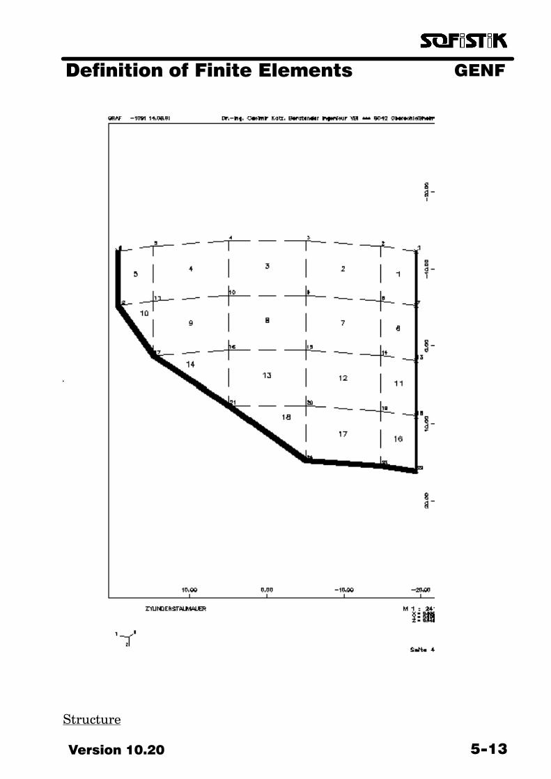
GENFDefinition of Finite Elements
5−13Version 10.20
Structure
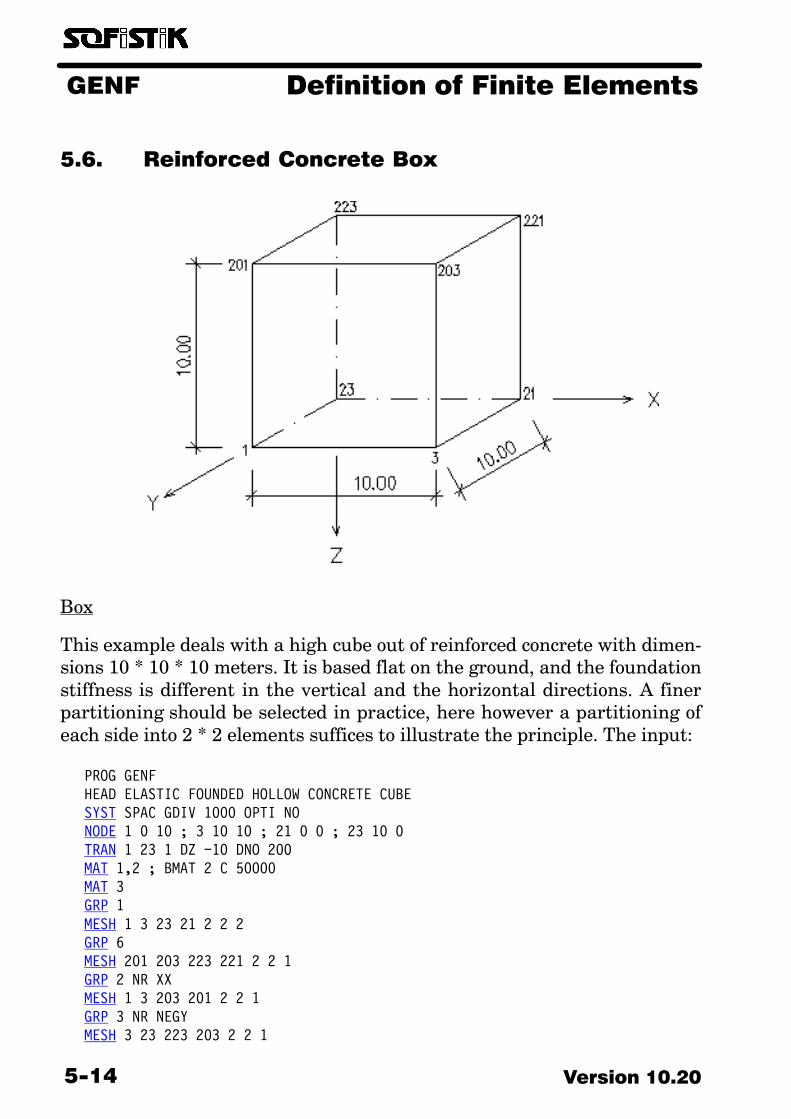
GENF Definition of Finite Elements
Version 10.205−14
5.6. Reinforced Concrete Box
Box
This example deals with a high cube out of reinforced concrete with dimen�sions 10 * 10 * 10 meters. It is based flat on the ground, and the foundationstiffness is different in the vertical and the horizontal directions. A finerpartitioning should be selected in practice, here however a partitioning ofeach side into 2 * 2 elements suffices to illustrate the principle. The input:
PROG GENF HEAD ELASTIC FOUNDED HOLLOW CONCRETE CUBE SYST SPAC GDIV 1000 OPTI NO NODE 1 0 10 ; 3 10 10 ; 21 0 0 ; 23 10 0 TRAN 1 23 1 DZ −10 DNO 200 MAT 1,2 ; BMAT 2 C 50000 MAT 3 GRP 1 MESH 1 3 23 21 2 2 2 GRP 6 MESH 201 203 223 221 2 2 1 GRP 2 NR XX MESH 1 3 203 201 2 2 1 GRP 3 NR NEGY MESH 3 23 223 203 2 2 1

GENFDefinition of Finite Elements
5−15Version 10.20
GRP 4 NR NEGX MESH 23 21 221 223 2 2 1 GRP 5 NR YY MESH 21 1 201 221 2 2 1 END
In order to subsequently interpret the stress resultants and the proportion�ing results correctly, it is important to select an appropriate coordinate sys�tem for the shell elements. The direction of the local X−axis is determined bythe input to the parameter NR of the MESH record, while the direction of theZ−axis is determined by the direction of rotation around the elements. Thison the other hand is determined by the sequence of the corner nodes in theinput of the MESH record. With the exception of the base plate, the local Z−axis always point to the interior of the box. This means that the lower rein�forcement layer lies at the inner side of the walls.
Since the stress resultants of shell structures are always local, they must becalculated at the nodes separately for each side of the cube. This is achievedby subdividing the structure into 6 groups. The group divisor (GDIV) in therecord SYST is set to 1000. During the element generation by the record MESHthe elements are assigned each time to the current group (record GRP) − theelement numbers are increased by the corresponding amount of thousands(see page after next).
In case of larger structures with more than 1000 nodes, duplicate elementnumbers may arise inside the groups. In such cases a negative MNO− valueshould be used in order to select a numbering that will be independent of thenode numbers.
M A X I M U M N O D A L P A R A M E T E R S max−No Xmin/Xmax Ymin/Ymax Zmin/Zmax 223 .000 .000 −10.000 10.000 10.000 .000
NODAL COORDINATES AND SUPPORTS Number X (m) Y (m) Z (m) Support Conditions 1 .000 10.000 .000 PY PZ 2 5.000 10.000 .000 3 10.000 10.000 .000 11 .000 5.000 .000 12 5.000 5.000 .000 13 10.000 5.000 .000 21 .000 .000 .000 22 5.000 .000 .000 23 10.000 .000 .000

GENF Definition of Finite Elements
Version 10.205−16
101 .000 10.000 −5.000 102 5.000 10.000 −5.000 103 10.000 10.000 −5.000 111 .000 5.000 −5.000 113 10.000 5.000 −5.000 121 .000 .000 −5.000 122 5.000 .000 −5.000 123 10.000 .000 −5.000 201 .000 10.000 −10.000 202 5.000 10.000 −10.000 203 10.000 10.000 −10.000 211 .000 5.000 −10.000 212 5.000 5.000 −10.000 213 10.000 5.000 −10.000 221 .000 .000 −10.000 222 5.000 .000 −10.000 223 10.000 .000 −10.000
M A T E R I A L S
No. 1 −−−−−−−−−−−−−−−−−−−−−−−−−−−−−−−−−−−−−−−−−−−−−−−−−−−−−−−−−−−−−−−−−−−−−−−− Young−module 30000 [MPa] Safetyfactor 1.00 [−] Poisson−Ratio .20 [−] Shear−module 12500 [MPa] Compress.module 16667 [MPa] Weight 25.0 [kN/m3] Weight buoyancy 15.0 [kN/m3] Temperat. coeff. 1.00E−05 [−]
No. 2 −−−−−−−−−−−−−−−−−−−−−−−−−−−−−−−−−−−−−−−−−−−−−−−−−−−−−−−−−−−−−−−−−−−−−−−− Young−module 30000 [MPa] Safetyfactor 1.00 [−] Poisson−Ratio .20 [−] Shear−module 12500 [MPa] Compress.module 16667 [MPa] Weight 25.0 [kN/m3] Weight buoyancy 15.0 [kN/m3] Temperat. coeff. 1.00E−05 [−]
No. 3 −−−−−−−−−−−−−−−−−−−−−−−−−−−−−−−−−−−−−−−−−−−−−−−−−−−−−−−−−−−−−−−−−−−−−−−− Young−module 30000 [MPa] Safetyfactor 1.00 [−] Poisson−Ratio .20 [−] Shear−module 12500 [MPa] Compress.module 16667 [MPa] Weight 25.0 [kN/m3]

GENFDefinition of Finite Elements
5−17Version 10.20
Weight buoyancy 15.0 [kN/m3] Temperat. coeff. 1.00E−05 [−]
E L A S T I C B E D D I N G No. Cs[kN/m3] Ct[kN/m3] pr[kN/m2] py[kN/m2] tan[−] c[kN/m2] w[kN/m3] 2 5.0000E+04 0.0000E+00 .00 .00 .00 .00 .0
F L A T E L E M E N T S EL−No Nodes MNo T(m) C(kN/m3) local−x (xyz) 1001 1 2 12 11 2 .200 5.000E+04H 1.000 .000 .000 1002 2 3 13 12 2 .200 5.000E+04H 1.000 .000 .000 1011 11 12 22 21 2 .200 5.000E+04H 1.000 .000 .000 1012 12 13 23 22 2 .200 5.000E+04H 1.000 .000 .000 2001 1 2 102 101 1 .200 1.000 .000 .000 2002 2 3 103 102 1 .200 1.000 .000 .000 2101 101 102 202 201 1 .200 1.000 .000 .000 2102 102 103 203 202 1 .200 1.000 .000 .000 3003 3 13 113 103 1 .200 .000 −1.000 .000 3013 13 23 123 113 1 .200 .000 −1.000 .000 3103 103 113 213 203 1 .200 .000 −1.000 .000 3113 113 123 223 213 1 .200 .000 −1.000 .000 4022 22 21 121 122 1 .200 −1.00 .000 .000 4023 23 22 122 123 1 .200 −1.00 .000 .000 4122 122 121 221 222 1 .200 −1.00 .000 .000 4123 123 122 222 223 1 .200 −1.00 .000 .000 5011 11 1 101 111 1 .200 .000 1.000 .000 5021 21 11 111 121 1 .200 .000 1.000 .000 5111 111 101 201 211 1 .200 .000 1.000 .000 5121 121 111 211 221 1 .200 .000 1.000 .000 6201 201 202 212 211 1 .200 1.000 .000 .000 6202 202 203 213 212 1 .200 1.000 .000 .000 6211 211 212 222 221 1 .200 1.000 .000 .000 6212 212 213 223 222 1 .200 1.000 .000 .000 H = Bedding normal (local z)
Lastly, the following figure shows a graph of the structure by GRAF with allnodes and element numbers, along with a graph of the structure with hiddenedges and the local element coordinate systems on the right.

GENF Definition of Finite Elements
Version 10.205−18
Box − Structure graph
5.7. Calotte Shell
The analysis of a calotte shell with quadrilateral elements is a sophisticatedFE−problem. It is obvious that one should arrange element edges along thelength and the width directions. This way, however, triangular elements re�sult at the North and the South Pole.
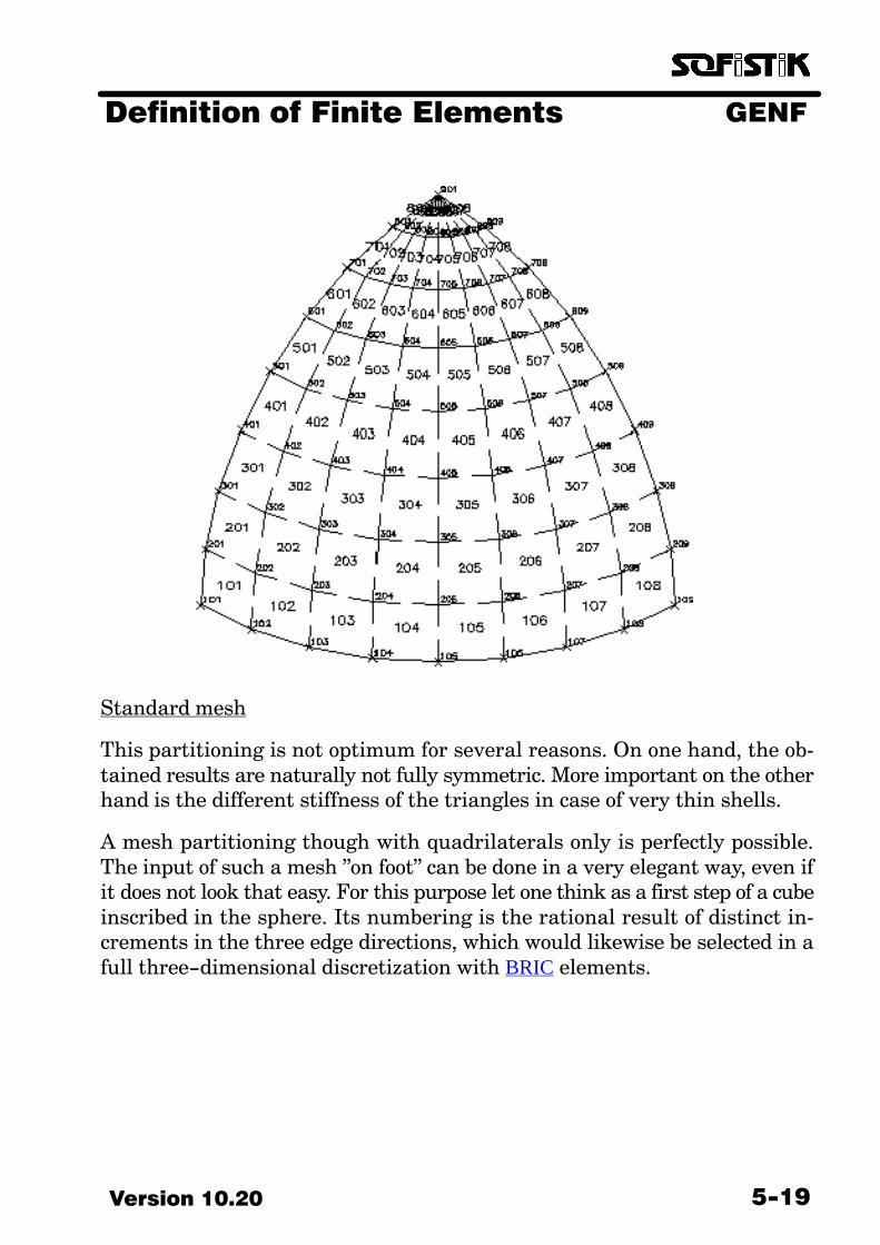
GENFDefinition of Finite Elements
5−19Version 10.20
Standard mesh
This partitioning is not optimum for several reasons. On one hand, the ob�tained results are naturally not fully symmetric. More important on the otherhand is the different stiffness of the triangles in case of very thin shells.
A mesh partitioning though with quadrilaterals only is perfectly possible.The input of such a mesh "on foot" can be done in a very elegant way, even ifit does not look that easy. For this purpose let one think as a first step of a cubeinscribed in the sphere. Its numbering is the rational result of distinct in�crements in the three edge directions, which would likewise be selected in afull three−dimensional discretization with BRIC elements.

GENF Definition of Finite Elements
Version 10.205−20
Cube in octants
As a next step all nodes are stretched radially onto the sphere surface. Un�fortunately, this is not a practical method because neither GENF nor MONETor AutoCAD offer such a function.
An alternative construction subdivides the sphere surface into 8 segments.Great circles are drawn from the piercing points of the eight space diagonalsto the corners of the spherical triangles. Each of these arcs can then be uni�formly subdivided, thus the total of the 24 quadrilaterals can be subdividedthrough great circles into n x n quadrilaterals.

GENFDefinition of Finite Elements
5−21Version 10.20
Great circles for mesh partitioning
A relatively easy method by means of CADINP has been presented here.
The transformation by means of spherical coordinates is a basic idea. The se�quence of the two rotation angles should not be overlooked, because it is criti�cal during a generation. A special transformation matrix of the incrementalrotation is employed therefore, instead of the classical spherical coordinates.If one subdivides all rotation angles into small increments and then rotatesin turn about one of the coordinate axes each time, one obtains a transform�ation which no longer depends on the sequence of rotations.
With the rotations φi = tanϕi the matrix of transformation is:
��������
1��2y �2
z� �CC�
�−z �SS�xy�CC�
y �SS�xz�CC�
z �SS�xy�CC�
1��2x �2
z� �CC�
−x�SS�yz�CC�
−y �SS�xz�CC�
x�SS�yz�CC�
1��2x �2
y� �CC�
��������
with
GENF Definition of Finite Elements
Version 10.205−22
ψ2 = φx2 + φy
2 + φz2
CC = (1−cosψ)/ψ2
SS = sinψ/ψ
if φx = 0, and the original vector is (1,0,0), then the resulting coordinates of therotation are:
| cosψ −φz·SS φy·SS |
A Macro is defined for the input, which defines the nodes of a quadrilateralfield each time. The starting point for the Macro is the X− axis, and rotationsof 45 degrees about the Y− and Z−axis take place each time. The other threefaces of an octant are described via cyclic interchange of the node labels.
The variable #90 stands for the chord angle ψ. During calculation of SS thespecial case ψ=0 must be controlled by a special LOOP, which should executeonly once or not at all.
PROG GENFHEAD QUAD−PARTITIONING OF A SPHERICAL SURFACEsyst spacMAT 1 e 2.1E8GRP 0 T 0.005
LET#4 4 $ Mesh partitioning (<9!)LET#9 10. $ Radius
$ DEFINE ALL ELEMENTS WITH A CUBENODE 101 #9 0 0 109 #9 #9 0 909 0 #9 0 181 #9 0 #9 189 #9 #9 #9 981 0 0 #9 989 0 #9 #9MESH 101 109 189 181 #4 #4 MNO 1 181 189 989 981 #4 #4 MNO 1 109 909 989 189 #4 #4 MNO 1NODE (1 109 1) fix pzzm ; (109 909 100) == (101 181 10) fix pyym ; (181 981 100) == (909 989 10) fix pxxm ; (989 981 −1) == 101,909,981 fix xpmm,ypmm,zpmm
$BLOCK BEG1

GENFDefinition of Finite Elements
5−23Version 10.20
$ SUBPROGRAM FOR NODE GENERATION IN A COORDINATE THIRD$ NODE COORDINATES WITH NONLINEAR INCREMENT ROTATION$ #1,#2,#3 = NODE NUMBER ON AXIS + INCREMENTSLET#10 0,45/#4 $ Starting value + Increment phi−YLOOP #4+1LET#20 0,45/#4 $ Starting value + Increment phi−ZLOOP #4+1LET#90 SQR(TAN(#10)**2+TAN(#20)**2)LET#91 ATN(#90)LET#92 COS(#91),0.0LOOP #91−0.001 ; LET#93 SIN(#91)/#90 ; ENDLOOP −1$ nodes #1 #9*#92 #9*TAN(#20)*#93 #9*TAN(#10)*#93LET#20 #20+#21LET#1 #1+#3ENDLOOPLET#10 #10+#11LET#1 #1−#3*(#4+1)+#2ENDLOOP$BLOCK END1LET#1 101,10,1 $ Node number + Increments of the X−SectorNODE NO X Y Z$BLOCK SET1LET#1 101+#4*101,−100,10 $ Node number + Increments of the Y−SectorNODE NO Y Z X$BLOCK SET1LET#1 101+#4*110,1,−100 $ Node number + Increments of the Z−SectorNODE NO Z X Y$BLOCK SET1END
The following values were selected for a comparison of the two mesh parti�tionings:
Radius R = 10.0 mThickness t = 5 mmE−Modulus E = 2.1E8 kN/m2
Poisson’s ratio µ = 0.2Loading p = 10 kN/m2 radial
n� �� p�R�2��� 50�kN�m
�R� �� n�E� t�
� �1��� �R� �� 0.381�mm
In the case of the mixed mesh, the results at the QUAD−corners are u = 0.380mm, n−xx = 49.83 kN/m2 and n−yy = 49.83 kN/m2. At the triangle’s corner
GENF Definition of Finite Elements
Version 10.205−24
though one obtains u = 0.843 mm, n−xx = 43.22 kN/m2 and n−yy = 65.55 kN/m2.
The present mesh results in the following values:
Partition 4 Partition 8Axes of coordinates (Node 101) 0.133 mm 0.363 mmBisecting line of the angle (Node 109) 1.280 mm 0.458 mmSpace diagonal (Node 189) 4.806 mm 0.388 mm
The stress resultants in the elements fluctuate in partition 8 from 45.30 upto 54.41 kN/m; the value on the axis of coordinates is 49.86 kN/m.
Opposite to the mixed mesh, the QUAD−elements generated in such mannerare unfortunately not perfectly plane any more, a fact that was neglectedearlier and led to excellent results. Starting from version 93 ASE takes thiseffect into consideration by means of eccentricities. The entire structure be�comes more flexible this way and a clear bulge is obtained along the space di�agonals in cases of coarse partitioning. The influence of the eccentricitiesdiminishes very fast by refining the mesh.
5.8. Examples in the Internet
Different statics examples are to be found in the Internet at www.sofis�tik.com/bibliothek.htm
![H20youryou[2] · 2020. 9. 1. · 65 pdf pdf xml xsd jpgis pdf ( ) pdf ( ) txt pdf jmp2.0 pdf xml xsd jpgis pdf ( ) pdf pdf ( ) pdf ( ) txt pdf pdf jmp2.0 jmp2.0 pdf xml xsd](https://img.dokumen.tips/doc/110x75/60af39aebf2201127e590ef7/h20youryou2-2020-9-1-65-pdf-pdf-xml-xsd-jpgis-pdf-pdf-txt-pdf-jmp20.jpg)