HAL Id: hal-02158803https://hal.archives-ouvertes.fr/hal-02158803

Submitted on 18 Jun 2019

HAL is a multi-disciplinary open accessarchive for the deposit and dissemination of sci-entific research documents, whether they are pub-lished or not. The documents may come fromteaching and research institutions in France orabroad, or from public or private research centers.

L’archive ouverte pluridisciplinaire HAL, estdestinée au dépôt et à la diffusion de documentsscientifiques de niveau recherche, publiés ou non,émanant des établissements d’enseignement et derecherche français ou étrangers, des laboratoirespublics ou privés.

Real Time Clock Skew Estimation over Network DelaysDominique Fober, Yann Orlarey, Stéphane Letz

To cite this version:Dominique Fober, Yann Orlarey, Stéphane Letz. Real Time Clock Skew Estimation over NetworkDelays. [Technical Report] GRAME. 2005. �hal-02158803�

GRAMELaboratoire de recherche en informatique musicale

Technical report TR-050601

Real Time Clock Skew Estimationover Network Delays

Dominique Fober, Yann Orlarey, Stephane Letz{fober,orlarey,letz}grame.fr

June 2005

GrameCentre National de Creation Musicale

9, rue du Garet BP 1185FR - 69202 Lyon Cedex 01

Abstract

Clock skew is one of the significant issues of real-time networking. We have previously proposed a newalgorithm for clock skew detection that operates one a one-way measurement, simply based on timestamped packets. This algorithm was initially targeted to Internet transport context. It has beenshowed that it is also suitable to low latency transport conditions using an adequate parameters set.This report presents improvements to the algorithm as well as as well as parameters characterization,along with the corresponding performance measurements.

1 Introduction

Works concerning clocks synchronization are numerous: whether developed in the context of distributedsystems or to provide a worldwide accurate common time, clock synchronization algorithms have reacheda mature level of performance. However, there are many cases where these algorithms are not applica-ble: peer to peer networking for example cannot benefit of the distributed systems methods, one-waytransmissions cannot support protocols like NTP (Network Time Protocol) [7]. There are also manyapplications that only needs to maintain a common time rate without concern about the clock offsets:Internet delays measurement for example have to separate the clock skew from actual transport delay;real-time multimedia streaming applications have to maintain a synchronized rate for data exchange.

However, there are a few works focusing on the clock skew estimation only. In network performancemeasurements domain, several algorithms have been developed to remove the clock skew from one-waydelay measurements [9] [11]. The most accurate of them is the Moon linear programming algorithm[9]. Almost of these algorithms are not applicable in real-time: the skew computation becomes rapidlyprohibitive when the time increases. Only the linear regression algorithm supports real-time with aconstant cost but since the deferred time version is not robust in presence of outliers, it performs evenworse in real-time.

In the multimedia domain, the problem is approached using techniques similar to NTP [2], or fre-quently ignored because it is avoided by talkspurt based systems, or naturally solved by adaptive playoutmechanisms. This latter solution is however not satisfying since the skew compensation produces signif-icant distortions.

Many techniques used to manage time are based on Phase Locked Loop like in NTP [8] or on DelayLocked Loop to filter time like in the jack audio system [1]. We have previously developed an algorithmnamed EPTMA (which stands for Exponential Peak Tolerant Midpoint Algorithm) [4], mostly inspiredby distributed systems CSA (Clock Synchronization Algorithms) but that is not so distant to NTP.

1

EPTMA operates on a one-way packets transmission and produces a real-time estimation of the receiverclock deviation in regard of the sender clock. It only relies on time stamped messages and may thereforeoperate over existing protocols like RTP [12]. It has been first designed for the Internet but also performsvery efficiently on a low latency network [6] using an adequate parameters set.

The idea behind the present work is to improve the algorithm by investigating in several directions:what are the best parameters suitable to a wide range of transport contexts? can adaptive parametersimprove the skew estimation? can technics developed in [8] or [1] benefit to the algorithm? this reportaims at providing replies to all these questions.

The rest of the paper is organized as follows. Section 2 introduces the skew estimation problem.Section 3 recalls the EPTMA functioning. Section 4 presents the methodology used to assess the algo-rithm performances. In section 5 we describe our strategy to improve the algorithm and we give thecorresponding performances, along with their correlation to the parameters set. We finally conclude insection 6.

2 The skew estimation problem

The figure 1 presents typical latency variations measured during a network audio session. The latencyvariation is expressed in audio frames. 4 different stations were broadcasting 128 frames audio bufferscollected at a 44.100 kHz sampling rate. The underlying network architecture was Ethernet 100 Mb. Theconstant increase slope drawn on the figure represents the clock skew; it may be viewed as the plot ofthe difference between the sender and the receiver clocks minus the clocks offset ie:

δ(t) = Cs(t)− Cr(t)− (Cs(0)− Cr(0)) where Cs and Cr represents the sender and receiver clocks.It has been obtained using the linear programming algorithm developed by Moon [9]. It exhibits a 36frames skew over the 3 minutes measurement, which represents about a 1 per 220 000 time unit deviation.The problem of the clock skew estimation may be viewed as the problem of the constant slope evaluation.

Figure 1: Typical mixed latency variation and clock skew.

Real-time skew estimation is a compromise between accuracy and inertia. Depending on the param-eters used, the algorithm may adapt quickly to the deviation slope but also produce distorted values ontransient transport changes, but it could also be less sensitive to local transport changes at the expense ofadditional time to detect the correct slope. The figure 2 clearly illustrates this compromise: the straight

2

line is the linear estimation previously shown by the figure 1, it represents the optimal detection slope.The first curve below is the output of a responsive estimation but that shows a significant distortionaround time 2”. The lower curve is a smoothed estimation that avoids almost of the distortion but takesabout 20 seconds to reach the correct slope: during this time, the clocks are drifting without any possiblecorrection, leading to potential problems with the audio rendering engine.

Figure 2: Clock skew estimation compromise.

3 EPTMA

The basic intuitive idea about EPTMA consists in selecting the mean values of the delay variations andto operate a smoothing of these values to obtain the clock skew estimation. The selection process makesuse of a sliding window. Let w be the window size and k the number of values retained per window, at atime t, the algorithm computes a sorted delay variation vector as: ∆w

t = [δt−w · · · δi · · · δt] , δi 6 δi+1

The highest and lowest values are discarded and the mean delay variation dm is then:

dm =1k

(w+k)/2∑i=(w−k)/2

δi 1 6 k 6 w (1)

At time t, the clock skew estimation st is finaly obtained by smoothing the mean delays using expo-nential averaging:

st = αdtm + (1− α)st−1 0 6 α 6 1 (2)

where α is the weighting factor.During the initialization stage (i.e. while the temporal window w isn’t complete), the algorithm

computes the mean delay values using a parabolic value for k, dynamically computed from the actualavailable values. Let n be the values count, the parabolic retained values rn is computed as:

rn = k − k

w2(n− w)2 0 < n < w (3)

3

4 Methodology

An important point, before presenting the possible improvements of the algorithm, concerns the way toassess these improvements. In this intent, we introduce a method to characterize the skew accuracy andwe describe the data set used for assessment.

4.1 Characterization of the skew estimation accuracy

The clock skew estimation is normalized in order to provide a common basis for characterization. Nor-malization consists in subtracting the optimal skew slope obtained as output of the linear programmingalgorithm, to the clock skew estimation. This is similar to evaluate clock deviations with perfectly fre-quency synchronized clocks: there is no skew and the optimal slope line is f(x) = 0. Accuracy of theestimation is then characterized by two figures that are directly related to the compromise mentioned insection 2:

• the responsiveness R: corresponds to the time necessary to reach the correct skew slope. Theresponsiveness is expressed in time unit deviations. It may be viewed as the deviation from theoptimal detection slope during the initial stage of the transmission. It depends obviously on theinitial transport context.

• the instability I: denotes the estimation curve stability after the initial stage. It is expressed intime units representing the range of the values after the initial stage. An optimal detection slopeshould converge to f(x) = n where n is the above responsiveness.

12

R

I

A

Figure 3: Normalized clock skew detections and corresponding stages.

The figure 3 shows normalized estimation curves (from figure 2) and illustrates their responsivenessand stability. Highlithed areas 1 and 2 correspond respectively to the responsiveness (∼ 2.5 frames) andstability (∼ 1 frame) of the smoothed estimation clock skew. The overall accuracy is about 3.5 frames.Concerning the upper curve, it may be considered as very responsive (no initial stage) but it behavesvery badly from accuracy viewpoint.

4

4.2 Data set

We have selected a set of 8 transport delay variations obtained from real transmissions over several kindof network and using different payloads. To collect the results we used the following methods:

• the unix tool ping : it has the advantage to give results with a known clock skew i.e. none

• an audio streaming application supporting several concurrent audio streams

• a MIDI streaming application [5].

Transport characteristics are summarized in table 1. The whole set is presented in appendix.

method network connection speed nameping general purpose Ethernet 10 Mb local 1

- isolated Ethernet 100 Mb local 2- Internet via adsl > 2 Mb adsl 1 & 2

audio streaming isolated Ethernet 100 Mb audio 1 & 2MIDI streaming Internet via modem 28.8 kbs midi 1 & 2

Table 1: Measurements methods and context

4.3 Data set normalization

The data set normalization consists in removing the clock skew, which is computed using the linearprogramming algorithm. This algorithm gives high quality results over the whole data set. Of course,the measures obtained using ping were not normalized since not subject to clock deviation. Normalizeddata set are flat and the corresponding optimal clock skew estimation should converge to f(x) = 0.

Next, measurement of the accuracy is achieved thru the following steps:

• a simulated clock skew varying from -0.003 to +0.003 by 0.001 step is applied to each normalizeddata,

• for each simulated slope, the skew estimation is computed, which produces a skew curve as output,

• this resulting curve is finally normalized back and the accuracy figures are computed as describedin section 4.1.

Each operation is repeated over the whole data set.

5 Improving the estimation accuracy

Several directions have been investigated with more or less success, to improve the results produced bythe EPTMA algorithm: using the DLL presented in [1] or a second order filter as defined in [3] in place ofthe exponential averaging, changing the first stage selection policy and exploring the parameters space.

5.1 The selection process

5.1.1 Mid point versus low point averaging

The first operation of the algorithm consists in discarding the highest and lowest delays to produce amean value from a subset of the medium delays. Results of the measurements show that using the lowestinstead of the medium delays produces better estimations, especially in the context of transient latencyincrease. The equation 1 is thus replaced by the low point averaging dl computed as:

dl =1k

k∑i=1

δi 1 6 k 6 w (4)

The figure 4 shows the increase of accuracy obtained using low point instead mid point averaging witha window size w = 200 and k = 10, on different delays data. The graphic plots the difference Am − Al

where Am and Al are respectively the mid point and the low point accuracies.

5

Figure 4: Mid point versus low point comparison: the graphic shows the accuracy difference between themid and low point averaging.

Results over the whole data set shows that equations 1 and 4 produce equivalent estimations for lowlatency and stable transport contexts. But in case of delay increase, the benefit of the low point averagingmay become very significant.

The intuitive interpretation of this behavior is the following: let’s consider that there are true andfalse delays. true delays are those that represent the minimum (or optimum) transport time, false delaysare those that include additional latency (mainly due to queuing). The first idea with the selectionprocess comes from the distributed systems that discard false information using a strategy proposed byLamport [10]. But there was a misconception concerning the discarded values: low delays are obviouslydenoting an information more close to the true delay than the medium ones.

5.1.2 Window size and retained values

The window size and the number of retained values have been explored with w varying from 10 to 300by 10 increment and k from 1 to 30. From the results obtained, it is obvious that a single value retainedper window is most of the time the most efficient solution. Therefore equation 4 can be simplified as:

dl = min(∆wt ) (5)

Concerning the window size, the larger the window is, the better are the results. In particular, a largewindow allows to cross a transient high latency period without distortion, provided that the period issmaller than the window size: for example, the accuracy on ADSL1 (see figure 10 in appendix) dropsdown from 6.8 to 1.2 when the window size increases from 220 to 230, simply because the initial highlatency period lasts over 225 points.

However, in the general case there is a size over which there is no significant improvement: for ourdata set, this window size is 250. But it is noteworthy that for stable low latency delays (such as LOCAL1and LOCAL2 see figure 11 in appendix), this size drops down to 20.

5.1.3 Initial stage

The EPTMA algorithm dynamically computes the count of retained values according to the availablevalues up to the window size (eq. 3). It appears that a better strategy consists in waiting for the

6

Figure 5: ADSL1 skew estimation with and without initial stage.

window completion before producing the estimation and to normalize this values to zero. The figure 5illustrates the difference: it corresponds to estimations computed from the ADSL1 data set (see figure 10in appendix) with a 0.003 skew. Without initial stage, the skew estimation over the first window w is:

s(i) = min [δ(1) · · · δ(w)] with 1 6 i 6 w

and with initialization stage:

s(i) = min [δ(1) · · · δ(10)] with 1 6 i 6 10s(i) = min [δ(1) · · · δ(i)] with 10 < i 6 w

5.2 Replacing the exponential averaging

We tried to use the DLL presented in [1] or a second order low pass filter in place of the exponentialaveraging. Input of the DLL or of the filter was the output of the first stage selection process. The DLLfunction is defined as:

y(n) = bx(n) + cx(n− 1)− (b− 1)y(n− 1)− cy(n− 2) (6)

with F sample frequency of the loopB required bandwith of the filter

andw = 2πB/F

b =√

2wc = w2

Using the adequate parameters, it behaves exactly as the exponential averaging function (eq. 2).We tried also to use a low pass second order filter defined as:

y(n) = b0x(n) + b1x(n− 1) + b2x(n− 2)− a1y(n− 1)− a2y(n− 2) (7)

with fc analog cut-off frequencyζ damping factor

7

fs sampling frequencyC = 1/[tan(πfc/fs)]

andb0 = 1/(1 + 2ζC + C2

b1 = 2b0

b2 = b0

a1 = 2b0(1− C2)a2 = b0(1− 2ζC + C2)

Although its behavior is slightly different, it produces results very similar to exponential averaging.

Figure 6: Weight parameter impact on the accuracy with different skews.

5.3 Exponential averaging parameters

The weight parameter α of the exponential averaging function given by equation 2 has been exploredthru the following set of values: [ 0.001, 0.003, 0.005, 0.008, 0.010, 0.015, 0.020, 0.030 ] . The figure6 gives one viewpoint over the results: it presents the mean accuracy obtained using different α valueswhen the skew is varying from -0.003 to 0.003. For these measures, the window size was w = 250. It isobvious from the results that a small α value gives better results when the skew is small but degradesvery significantly when the skew increases.

This view however masks the particularities of the different data sets: the best results are actuallyobtained using α values varying from 0.003 to 0.03, depending on the delays shape. To get a finer view onthe results, we need to differentiate the responsiveness and the stability. The figure 7 shows normalizedestimation curves computed using the ADSL2 data set (see figure 10 in appendix) with α values varyingfrom 0.001 to 0.02 and applied to a +0.003 and -0.003 deviations. The graphic clearly illustrates a non-obvious point: positive and negative deviation slopes produce asymmetric results regarding accuracy. Inparticular, for ascending deviations, instability is generally covering the responsiveness area so that theaccuracy A is not R + I and could likely be max(R, I). On the contrary, for descending deviations, we’llgenerally have R < A < R + I. It is also clear from the results that the responsiveness is an issue onlyfor weight parameter α < 0.005.

Actually, using α = 0.008 gives the best results over the whole data set. The figure 8 presents themean accuracy obtained over the data set with the distance to the best α value for each deviation. Asexpected, the distance is maximal for 0 deviation but very small anywhere else.

8

Figure 7: Normalized skew estimations with varying α factor.

Figure 8: Mean accuracy and distance to optimal values using α = 0.008.

9

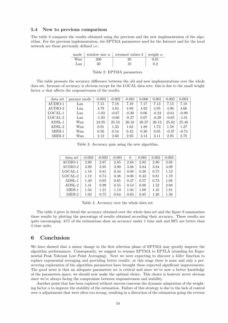
5.4 New to previous comparison

The table 3 compares the results obtained using the previous and the new implementation of the algo-rithm. For the previous implementation, the EPTMA parameters used for the Internet and for the localnetwork are those previously defined i.e.:

mode window size w retained values k weight αWan 200 20 0,01Lan 30 10 0.2

Table 2: EPTMA parameters.

The table presents the accuracy difference between the old and new implementations over the wholedata set. Increase of accuracy is obvious except for the LOCAL data sets: this is due to the small weightfactor α that affects the responsiveness of the results.

data set params mode -0.003 -0.002 -0.001 0.000 0.001 0.002 0.003AUDIO-1 Lan 7.15 7.18 7.19 7.17 7.13 7.15 7.18AUDIO-2 Lan 4.79 4.84 4.89 4.92 4.95 4.96 4.66LOCAL-1 Lan -1.03 -0.67 -0.30 0.06 -0.24 -0.61 -0.99LOCAL-2 Lan -1.03 -0.66 -0.27 0.07 -0.29 -0.65 -1.01

ADSL-1 Wan 24.95 25.53 26.16 26.37 26.13 25.82 25.48ADSL-2 Wan 0.91 1.33 1.62 1.80 1.73 1.58 1.27MIDI-1 Wan 0.56 0.54 0.42 0.30 0.05 -0.37 -0.74MIDI-2 Wan 2.12 2.60 2.93 3.13 3.11 2.95 2.78

Table 3: Accuracy gain using the new algorithm.

data set -0.003 -0.002 -0.001 0 0.001 0.002 0.003AUDIO-1 2.90 2.87 2.85 2.88 2.92 2.90 2.88AUDIO-2 3.99 3.95 3.90 3.86 3.84 3.84 4.09LOCAL-1 1.18 0.81 0.44 0.08 0.38 0.75 1.13LOCAL-2 1.12 0.74 0.38 0.06 0.43 0.81 1.19

ADSL-1 1.40 0.95 0.65 0.47 0.57 0.73 1.08ADSL-2 1.41 0.99 0.55 0.54 0.98 1.52 2.08MIDI-1 1.34 1.21 1.13 1.04 1.08 1.45 1.81MIDI-2 1.03 0.75 0.64 0.63 0.85 1.20 1.56

Table 4: Accuracy over the whole data set.

The table 4 gives in detail the accuracy obtained over the whole data set and the figure 9 summarizesthese results by plotting the percentage of results obtained according their accuracy. These results arequite encouraging: 41% of the estimations show an accuracy under 1 time unit and 98% are better than4 time units.

6 Conclusion

We have showed that a minor change in the first selection phase of EPTMA may greatly improve thealgorithm performances. Consequently, we suggest to rename EPTMA to EPTLA (standing for Expo-nential Peak Tolerant Low Point Averaging). Next we were expecting to discover a killer function toreplace exponential averaging and providing better results: at this stage there is none and only a per-severing exploration of the algorithm parameters have brought these expected significant improvements.The good news is that an adequate parameters set is critical and since we’ve now a better knowledgeof the parameters space, we should now make the optimal choice. This choice is however never obvioussince we’re always facing the compromise between responsiveness and stability.

Another point that has been explored without success concerns the dynamic adaptation of the weight-ing factor α to improve the stability of the estimation. Failure of this strategy is due to the lack of controlover α adjustments that were often too strong, resulting in a distortion of the estimation going the reverse

10

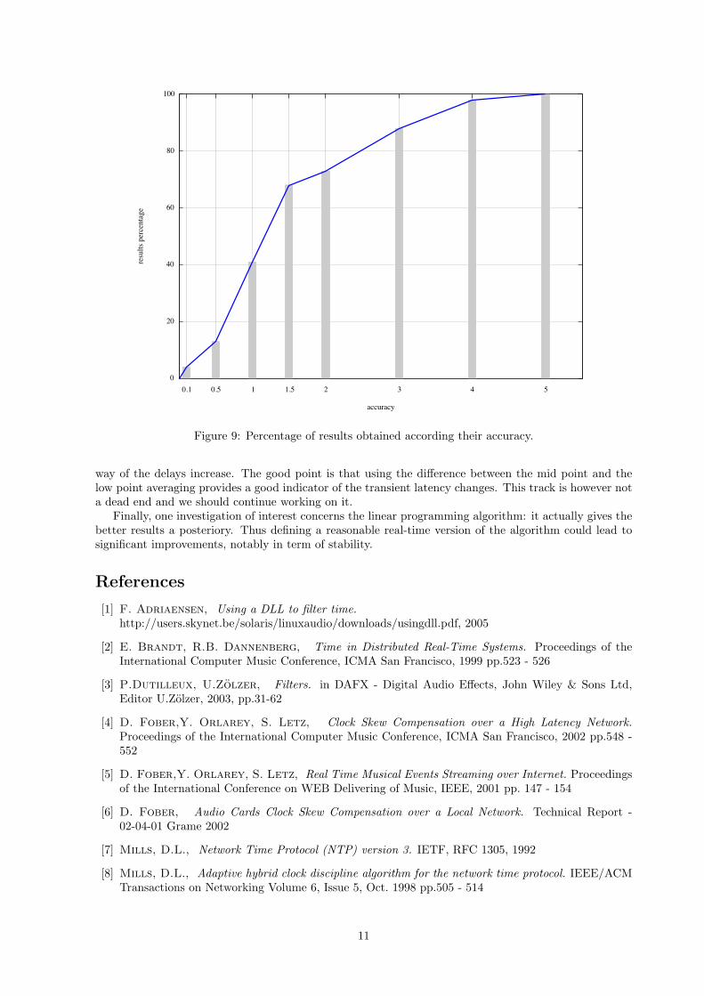
Figure 9: Percentage of results obtained according their accuracy.

way of the delays increase. The good point is that using the difference between the mid point and thelow point averaging provides a good indicator of the transient latency changes. This track is however nota dead end and we should continue working on it.

Finally, one investigation of interest concerns the linear programming algorithm: it actually gives thebetter results a posteriory. Thus defining a reasonable real-time version of the algorithm could lead tosignificant improvements, notably in term of stability.

References

[1] F. Adriaensen, Using a DLL to filter time.http://users.skynet.be/solaris/linuxaudio/downloads/usingdll.pdf, 2005

[2] E. Brandt, R.B. Dannenberg, Time in Distributed Real-Time Systems. Proceedings of theInternational Computer Music Conference, ICMA San Francisco, 1999 pp.523 - 526

[3] P.Dutilleux, U.Zolzer, Filters. in DAFX - Digital Audio Effects, John Wiley & Sons Ltd,Editor U.Zolzer, 2003, pp.31-62

[4] D. Fober,Y. Orlarey, S. Letz, Clock Skew Compensation over a High Latency Network.Proceedings of the International Computer Music Conference, ICMA San Francisco, 2002 pp.548 -552

[5] D. Fober,Y. Orlarey, S. Letz, Real Time Musical Events Streaming over Internet. Proceedingsof the International Conference on WEB Delivering of Music, IEEE, 2001 pp. 147 - 154

[6] D. Fober, Audio Cards Clock Skew Compensation over a Local Network. Technical Report -02-04-01 Grame 2002

[7] Mills, D.L., Network Time Protocol (NTP) version 3. IETF, RFC 1305, 1992

[8] Mills, D.L., Adaptive hybrid clock discipline algorithm for the network time protocol. IEEE/ACMTransactions on Networking Volume 6, Issue 5, Oct. 1998 pp.505 - 514

11

[9] Sue B. Moon, Paul Skelly, Don Towsley, Estimation and Removal of Clock Skew fromNetwork Delay Measurements. Proceedings of 1999 IEEE INFOCOM, New York, NY, March 1999,pp.227 - 234

[10] L. Lamport, R. Shostak, M. Pease, The Byzantine Generals Problem. ACM Transactions onProgramming Languages and Systems, Vol. 4, No. 3, July 1982, pp.382-401.

[11] V. Paxson, On Calibrating Measurements of Packet Transit Times. Proceedings of SIGMETRICS’98, June 1998

[12] Schulzrinne, H., Casner, S., Frederick, R. & Jacobson, V., RTP : A Transport Protocolfor Real-Time Applications. RFC 3550, IETF, 2003.

12

Appendix 1: measurements set

ADSL-1

ADSL-2

Figure 10: Ping measurements over Internet via adsl. The first transmission exhibits a high delay periodat the session start time. The second transmission shows a significant delay increase starting at hour 5.

LOCAL-1

LOCAL-2

Figure 11: Ping measurements over a local Ethernet network. The first transmission has been measuredon a general purpose 10Mb Ethernet network. The second transmission has been measured on Ethernet100Mb isolated by a switch.

13

AUDIO-1

AUDIO-2

Figure 12: Audio buffers transmission over Ethernet. 4 different stations were involved. Measurementsof 2 stations are presented along with the corresponding normalized delays.

MIDI-1

MIDI-2

Figure 13: MIDI transmission over Internet via a modem line. For the second transmission, note thelatency change starting at 3”. Note also that the normalized delays are not plotted because they werenot significant.

14

Appendix 2: EPTLA scilab code

//-------------------------------------------------------------// the eptla algorithm// parameters:// - x : a vector of latency variations// - win : the sliding window size// - w : the exponential averaging weighting factor// result:// - y : the clock deviations vector//-------------------------------------------------------------

function y=eptla(x, win, w)n=length(x);low=min(x(1:win));y=[ones(1:win)’*low; zeros(1:n-win)’];for i=win+1:n

low=min(x(i-win:i));y(i)=w*low + (1-w)*y(i-1);

endendfunction

15