3. Clock skew - bibing.us.esbibing.us.es/proyectos/abreproy/11286/fichero/1... · Luis Manuel Santana Gallego 31 Investigation and simulation of the clock skew in modern integrated

Luis Manuel Santana Gallego 31 Investigation and simulation of the clock skew in modern integrated circuits

3. Clock skew

3.1. Definitions

For two sequentially adjacent registers, as shown in figure 2.1, Ci and Cf are the

clock signals that drive the local data path. Both clock signals are generated in the same

clock source. The propagation delay of the clock signals from the source to the registers

Ri and Rf, is TCi and TCj respectively. They define the timing reference of when the data

signals leave each register. There is a clock distribution network designed to generate a

specific signal waveform. Ideally, clock events occur at all registers simultaneously.

Given this strategy of global clocking, the clock signal arrival time to each register is

defined with respect to a universal time reference.

The difference in clock signals arrival time between two register sequentially

adjacent is the clock skew Tskew. We can define the clock skew mathematical expression

as: Tskew = TCi – TCf. If the signals Ci and Cf are in complete synchronism, it means they

arrive at the exact same moment, the clock skew is zero. It is important to note that the

clock skew between is only relevant to sequentially adjacent registers that make up a

local data path. Thus, the clock skew, at system or chip level, between two registers

non-sequentially adjacent has no effects on the performance and reliability of a

synchronous digital system from an analysis viewpoint.

Different clock signal paths can have different delays due to several reasons. We can

summarize them in the following three reasons:

1) Differences in the wire lengths from the clock source to the clocked registers.

2) Differences in the delays of any active buffer in the clock distribution network.

3) Differences in the interconnection passive parameters.

We can note that, for a well-designed balanced clock distribution network,

distributed buffers are the primary clock skew source.


Clock skew magnitude and polarity have two different effects on system

performance and reliability. Depending on which signal, Ci or Cf, arrive earlier and the

magnitude of Tskew with respect to data path time delay TPD, system reliability and

performance can be degraded or improved. Both cases are discussed below.

1) Maximum data path/clock skew constraint relationship

If the clock signal arrival time to the final register, TCf, is previous to the arrival time

to the initial register, TCi, the clock skew is positive (TCi > TCf). Under this condition the

maximum operation reachable frequency is decreased. A positive clock skew is the

additional time amount that must be added to the minimum clock period to apply a new

clock signal edge to the final register without any problem.

Figure 3.1: Positive clock skew.

For a specific design, the greatest propagation delay TPD (max) of any local data

path between two sequentially adjacent registers must be less than the minimum clock

period TCP (min).

( )log int(max) (max)skew CP PD CP C Q ic setupT T T T T T T T−

≤ − = − + + + , where Ci CfT T> (3.1)

This situation is the typical analysis of the critical data path in a synchronous

system. If this constraint is not satisfied, the system will not operate correctly with this

specific clock period. Therefore, TCP must be increased if we want the circuit operates

without any problem. In a circuit where the clock skew tolerance is small, data and

clock signals should run in the same direction, thereby forcing that Ci leads Cf and

making the clock skew negative.


2) Minimum data path/clock skew constraint relationship

If the clock signal arrival time to the final register, TCf, is later than arrival time to

the initial register, TCi, the clock skew is negative (TCi < TCf). It can be used to improve

the maximum performance of a synchronous system by the reduction of the critical data

path. However, there is a minimum constraint to avoid race conditions.

Figure 3.2: Negative clock skew.

When Cf follows to Ci, clock skew must be less than the required time for the data

signal to leave the initial register, propagate through the combinatorial logic and

interconnections and setup in the final register input. If this condition is not met, the

data stored in the final register is overwritten with the data that was stored in the initial

register because it arrives to the Rf input earlier than the clock signal (race condition).

Furthermore, a circuit operating close to this restriction could not work correctly at

unpredictable times due to environmental temperature or power supply voltage

fluctuations:

log int(min) (min)PD C Q ic setupTskew T T T T T−

≤ = + + + , where Ci CfT T< (3.2)

where TPD (min) is the minimum data path delay between two sequentially adjacent

registers.

3.2. Clock skew sources

Clock skew appears due to differences in clock paths from the source to each

destination register. These differences can be unequal wire lengths or different resistive

and/or capacitive wire parameters. In a balanced clock tree, the nominal value for clock


skew is zero, since clock paths are designed to be equal. However, clock skew

appearance is still possible due to variations in the clock paths caused by process and

circuit parameter tolerances. We can classify them in the following way:

• Transistor parameter variations

In the integrated circuit fabrication process, all transistor parameters are subject to

deviations from their nominal values. Statistical models have been developed for

transistor parameters such as threshold voltage (VT), gate oxide thickness (tox), charge

carrier mobility (µ), transistor width (W) and effective channel length (∆Leff).

Figure 3.3: Vertical section of a MOS transistor.

In table 3.1, typical values for this parameter are presented according to different

technologies. In table 3.2, standard deviations are shown.

Parameter 130 nm 100 nm 70 nm 45 nm

VT 0.19 V 0.15 V 0.06 V 0.021 V

Tox 3.3 nm 2.5 nm 1.6 nm 1.4 nm

Leff 130 nm 100 nm 70 nm 45 nm

W (min) 130 nm 100 nm 70 nm 45 nm

Table 3.1: Typical values for different technologies [ITRS].


Parameter Description Standard Deviation

σVT Threshold voltage 4.2 %

σµ Charge carrier mobility 2 %

σtox Gate oxide thickness 1.3 %

σW Transistor width 5%

σLeff Transistor effective channel length 5 %

Table 3.2: Typical values for standard deviations [KAH-01].

• Interconnect Parameter Variations

Interconnect width (Wint) and thickness (tint) and interlevel dielectric thickness (TILD)

variations are the main parameters of interest. As technology advances, the number of

interconnect layers increases, and the interconnect lines become more non-uniform.

This non-uniformity, which is caused by manufacturing processes, produces large

variations of interconnect parameter values.

Figure 3.4: Interconnect segment main parameters.

In table 3.3, some typical values for this parameter are presented according to

different technologies. In table 3.4, standard deviations are shown.



Wint (min) 335 nm 237 nm 160 nm 103 nm

tint (min) 670 nm 500 nm 352 nm 235 nm



σWint Wire width 3 %

σtint Wire thickness 3 %

σTILD ILD thickness 3 %

Table 3.4: Typical values for standard deviations [FAN-98].

• System Parameter Variations

Besides process parameter variations, which are mainly the tolerances of device and

interconnect physical parameters, system level fluctuations may create clock skew.

Power supply voltage fluctuation (VDD) and temperature variations (T) are considered as

system level parameter variations.

In table 3.5, some typical values VDD are presented according to different

technologies. In table 3.6, standard deviations are shown.


VDD 1.2 V 1 V 0.9 V 0.6 V



σVDD Power supply voltage 3.3 % [KAH-01]

σT Temperature 8 % [GRO-98]

Table 3.6: Typical values for standard deviations.

The thermal image of the Alpha 21064 microprocessor, presented in section

2.4.1, shows a 30º C temperature gradient over the entire chip that gives a temperature

variation of about 8 % [GRO-98]. In figure 3.6, this image is depicted.


Figure 3.6: 20164 thermal image [GRO-98].

3.3. Clock skew models

An important research area in VLSI circuits is timing analysis, where simplified

models are used to estimate the delay through a CMOS circuit according to process and

circuit parameter variations. At first, a probabilistic model for the accumulation of clock

skew in synchronous systems is described. Using this model, upper bounds for expected

skew and its variance in tree distribution systems are derived. Thereafter, a model for

tapered H-Tree is described, where no buffers are placed at branching points and the

wires are widened to avoid reflections. The clock skew is calculated as function of

device, system and interconnect parameter variations. The first statistical model (upper

bounds model) is too conservative for estimating the clock skew of a well-balanced H-

tree clock distribution network because correlation between overlapped parts of paths

are not considered. Finally, a new approach to estimate the mean value and variance of

clock skew is described taking into account this correlation.

3.3.1. MODEL 1: Statistical model to estimate upper bounds of clock skew

This model is described in depth in Appendix 1.

Kugelmass and Steiglitz [KUG-88] present a probabilistic model for the

accumulation of clock skew in synchronous systems. Using this model, it’s possible to


estimate upper bounds for expected clock skew between processing elements (and its

variance) in symmetric tree distribution systems with N synchronously clocked

processing elements.

The first assumption in this model is the topology of the clock distribution network.

It must be a symmetric tree-like structure with a single source and N end points called

processing elements (PE). There must be only one path from the source to the PEs.

Figure 3.7: Model 1 tree structure.

Each clock path is composed of delay elements: buffers and interconnection wires.

It is possible to associate a random variable to each element that gives the delay

contribution of it. The total delay from the clock source to each PE is the sum of all the

random variables along the path. By the Central Limit Theorem, the sum converges to a

normal distribution.

According to these authors, it is possible to define a random variable that

characterizes the clock skew of the clock distribution network. It is R = Amax - Amin,

where Amax and Amin are the maximal and the minimal arrival time to any of the N PEs.

Random variables that compose R are dependent in a clock tree because they are

sums of overlapping variables. However, thanks to a demonstrated theorem, the


expected mean value of R is smaller than the same case but with independent random

variables.

Another theorem says that if R is composed of N independent identically distributed

random variables (it is the case for a symmetric clock distribution network), then, the

asymptotically expected value of R is:

[ ] ( )12

4ln ln ln ln 4 2 1

log2ln

N N CE R O

NN

πσ − − + = +

(3.3)

where C ≈ 0.5772 is Euler constant and σ is the standard deviation of the path delay.

The variance of R is given by:

[ ] 2 2

2

1

ln 6 logVar R O

N N

σ π = + (3.4)

Equation (3.3) is therefore asymptotic upper bound on the expected skew in a clock

distribution tree with N leaves.

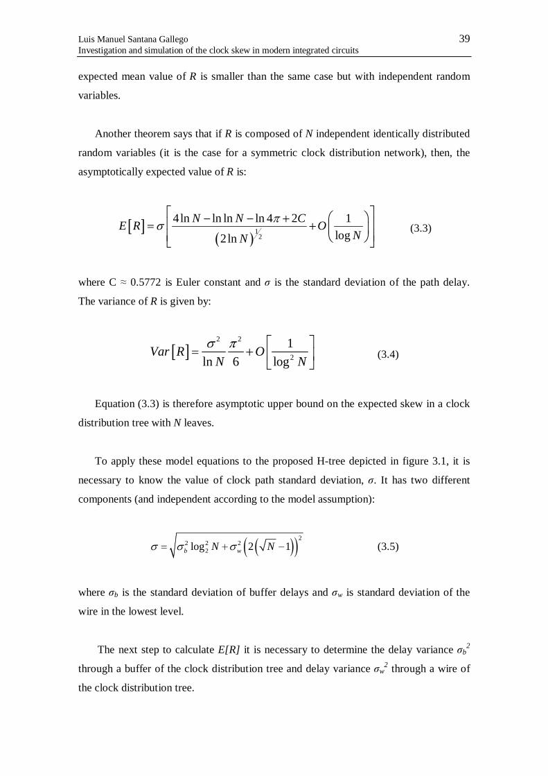
To apply these model equations to the proposed H-tree depicted in figure 3.1, it is

necessary to know the value of clock path standard deviation, σ. It has two different

components (and independent according to the model assumption):

( )( )22 2 2

2log 2 1b wN Nσ σ σ= + − (3.5)

where σb is the standard deviation of buffer delays and σw is standard deviation of the

wire in the lowest level.

The next step to calculate E[R] it is necessary to determine the delay variance σb2

through a buffer of the clock distribution tree and delay variance σw2 through a wire of

the clock distribution tree.


Using Sakurai’s model for interconnection delay, described in section 2.3.1, and the

possible clock skew sources considered by the authors (VT, tox, Leff, VDD, TILD, Wint, tint),

the value of σb2 and σw

2 is determined, in terms of variances of the independent random

variables that compose them, by the following expressions:

222 2

2 2 2 2 2

T ox eff DD

Delay Delay Delay Delayb V t L V

T ox eff DD

T T T T

V t L Vσ σ σ σ σ

∂ ∂ ∂ ∂ = + + + ∂ ∂ ∂ ∂ (3.6)

int int

2 22

2 2 2 2

int intILD

Delay Delay Delayw T W t

ILD

T T T

T W tσ σ σ σ

∂ ∂ ∂ = + + ∂ ∂ ∂ (3.7)

where:

( )( ) ( )

( )

0 00 int

0

0 0 0 00 int 0 int

0 0

0 0 00 int

0 0

2.30

2.30 2.30

2.30 2.3

Delay Delay

T T DD T

Delay Delay Delay

ox ox ox ox ox

Delay Delay Delay

eff eff eff eff

T T R RC C

V R V V V

T T TR C R CC C R R

t R t C t t t

T T TR C RC C

L R L C L L

∂ ∂ ∂= = +∂ ∂ ∂ −∂ ∂ ∂∂ ∂= + = + + +∂ ∂ ∂ ∂ ∂

∂ ∂ ∂∂ ∂= + = + +∂ ∂ ∂ ∂ ∂ ( )

( )

00 int

0 00 int

0

0

2.30

eff

Delay Delay

DD DD DD T

CR R

L

T T R RC C

V R V V V

+

∂ ∂ ∂= = +∂ ∂ ∂ −

(3.8)

( )

( ) ( )

int intint 0

int

int int int intint 0 int 0

int int int int int int int

int

int int int

1.02 2.30

1.02 2.30 1.02 2.30

Delay Delay

ILD ILD ILD

Delay Delay Delay

Delay Delay

T T C CR R

T C T T

T T TR C R CC C R R

W R W C W W W

T T R

t R t

∂ ∂ ∂= = +∂ ∂ ∂∂ ∂ ∂∂ ∂= + = + + +∂ ∂ ∂ ∂ ∂∂ ∂ ∂=∂ ∂ ∂ ( ) int

int 0int

1.02 2.30R

C Ct

= +

3.3.2. MODEL 2: Statistical model for clock skew in tapered H-trees


Zarkesh-Ha, Mule’ and Meindl [ZAR-98] described a compact model to enable

first-order estimation for clock skew in tapered H-trees. In this kind of structure, there


are not intermediate buffers at the split points and the wires must be widened to avoid

reflections in those points.

Figure 3.8: Model 2 tree structure [ZAR-98].

Authors propose that any H-tree circuit can be simplified in the following equivalent

circuit shown in figure 3.9.

Figure 3.9: Equivalent circuit of clock H-tree network [ZAR-98].

Using the equivalent circuit, the delay of the entire clock network of figure 3.9 is

divided into two parts:

• Interconnect delay from the clock source to clock the driver: If the H-tree network

is driven by a single driver, then the delay expression for a distributed RC line using

Sakurai’s model (50% of time delay) is:

2

2

2 2int 0

1 10.4 1 1

2 2

rrH tree n n

ILD

T D Dt T c

ερ ε−

⋅= ⋅ ⋅ ⋅ − + ⋅ ⋅ − ⋅ (3.9)


where εr is the relative dielectric constant of the ILD material, ρ the line resistivity,

co the speed of light in free space, D the die size, and n the number of H-tree levels.

• Transistor delay of the sub-block clock driver: the delay expression is according to

Sakurai’s Model (50% of time delay):

( )/

0.7 effdriver L

ox DD T

L WT C

C V Vµ = ⋅ ⋅ ⋅ ⋅ −

(3.10)

where CL is the capacitive load of the sub-block clock driver.

The overall delay of the entire clock distribution network is the sum of the previous

components: TDelay = TH-tree + TDriver. This model gives first order estimation of the

clock skew:

( ) DelayCSK Delay

TT x T x

x

∂= ∆ ≈ ∆

∂ (3.11)

where x is any variation of clock skew components such as ∆VT, ∆tox, ∆Leff , ∆Hint,

∆TILD, ∆VDD, ∆T and ∆CL. Table 3.1 shows the closed form equations for each

individual clock skew component by using (3.11):

Physical parameter

and derivation used

Clock skew component

Threshold voltage

fluctuation 0( ) 0.7 T T

CSK T LDD T T

V VT V R C

V V V

∆= ⋅ ⋅ ⋅ ⋅ −

Gate oxide thickness

tolerance 0( ) 0.7 ox

CSK ox L

ox

tT t R C

t

∆= ⋅ ⋅ ⋅

Transistor channel length

tolerance 0( ) 0.7 eff

CSK eff L

eff

LT L R C

L

∆= ⋅ ⋅ ⋅

Wire thickness

variation ( )

2

2 intint int int

2 int

1( ) 0.4 1

2CSK n

tT t r c D

t

∆= ⋅ ⋅ ⋅ ⋅ − ⋅


ILD thickness

variation ( )

2

2int int

2

1( ) 0.4 1

2

ILDCSK ILD n

ILD

TT T r c D

T

∆= ⋅ ⋅ ⋅ ⋅ − ⋅

IR drop 0( ) 0.7 DD DD

CSK DD LDD T DD

V VT V R C

V V V

∆= ⋅ ⋅ ⋅ ⋅ −

Non uniform register

distribution 0( ) 0.7 L

CSK L LL

CT C R C

C

∆= ⋅ ⋅ ⋅

Temperature

gradient 0

/( ) 0.7 g T

CSK LDD T

E q VT R C

V V

+ ∆ΤΤ = ⋅ ⋅ ⋅ ⋅ − Τ

Table 3.1: Clock skew components.

It is important to note that the model equations can be easily modified to be more

similar to other models, where the Sakurai’s expressions are used with 90% of time

delay. It only supposes to change the coefficients de TH-tree and TDriver.

- 2int int

0

: 0.4 1.02 1.02 ( ) rH tree H treeT T r c l l

c

ε− −

→ ⇒ = ⋅ ⋅ + ⋅

- 0: 0.7 2.3 2.3driver driver LT T R C→ ⇒ = ⋅ ⋅

3.3.3. MODEL 3: Statistical model for clock skew considering path

correlations


Jiang and Horiguchi [JIA-01] propose a new approach to estimate the mean value

and variance of clock skew for general clock distribution networks. The novelty is that

clock paths can be not identical and path delay correlation caused by the overlapped

parts of path lengths is considered. In this way, clock skew mean and variance is

accurately estimated for general clock distribution networks.

Clock paths of a clock distribution network usually have some common branches

over their length. These common branches cause correlation among the delays of these

paths. Only the overlapped parts of two paths determine the correlation between them.


If ξ is the maximum value of the propagation delay and η the minimum value, then

the mean value and the variance of the clock skew, χ, are given by:

( ) ( ) ( )E E Eχ ξ η= − (3.12)

( ) ( ) ( ) 2 ( ) ( )D D D D Dχ ξ η ρ ξ η= + − ⋅ (3.13)

Here, E(·) and D(·) represent the mean value and the variance of a random variable,

respectively, and ρ is the correlation coefficient of ξ and η. Author propose a recursive

approach for evaluating the parameters E(ξ), E(η), D(ξ), D(η) and ρ. Based on this

algorithm, an expression can be derived for the clock skew of a well-balanced H-tree

clock distribution networks.

• Clock skew estimation for H-tree clock distribution networks

Before developing the models, the H-tree itself must first be defined. The H-tree

presents intermediate buffers at each branching point and, without loss of generality, it

has n hierarchical levels, where n denotes the tree depth. The level 0 branch corresponds

to the root branch, and level n branches to the branches that support sinks. A level i

branch begins in a level split i point and ends in a level i+1 split point. The H-tree

illustrated in figure 3.10 is drawn for n=4 and it is used to distribute the clock signals to

16 processors.

Figure 3.10: A well-balanced H-tree clock distribution network for 16 processors.


For a n level well-balanced H-tree, let di, i=0, …, n be the actual delay of branch i of

a clock path. The clock skew E(χ) and skew variance D(χ) of the n level well-balanced

H-tree are given by:

( ) ( )1

1 1

2 1kn i

n i ki k

E D dπχππ

−

− += =

− = ⋅ ∑ ∑ (3.14)

( ) ( ) ( )0

12 1

in

ii

D D dπχ ρπ=

− = ⋅ − ⋅ ⋅ ∑ (3.15)

The closed-form expressions (3.14)–(3.15) indicate clearly how the clock skew is

accumulated along the clock paths and with the increase of H-tree size.

• Clock skew calculation in function of its components

The delay of a branch may then be obtained by averaging the rise and fall times

using Sakurai’s model for interconnection delays (90 % of time delay), described before

in section 2.3.1.

One approach to calculating the delay variance of a branch due to the variations of

process parameters is express the parameter relations in terms of independent variables.

Authors consider the following variables to calculate the variance of the delay of any

branch D(dn-i+k): VT, µ, tox, Leff, W, TILD, Wint, tint. The variance of the delay in a branch is

the following:

int int

222 2 2

2 2 2 2 2 2

2 22

2 2 2

int int

Delay T ox eff

ILD

Delay Delay Delay Delay DelayT V t L W

T ox eff

Delay Delay DelayT W t

ILD

T T T T T

V t L W

T T T

T W t

µσ σ σ σ σ σµ

σ σ σ

∂ ∂ ∂ ∂ ∂ = + + + + ∂ ∂ ∂ ∂ ∂ ∂ ∂ ∂ + + + ∂ ∂ ∂

(3.16)

where:


( )

( )

( ) ( )

0 00 int

0

0 00 int

0

0 0 0 00 int 0 int

0 0

0

0

2.30

2.30

2.30 2.30

Delay Delay

T T DD T

Delay Delay

T

Delay Delay Delay

ox ox ox ox ox

Delay Delay

eff eff

T T R RC C

V R V V V

T T R RC C

V R

T T TR C R CC C R R

t R t C t t t

T T R

L R L

µ µ

∂ ∂ ∂= = +∂ ∂ ∂ −∂ ∂ ∂= = +∂ ∂ ∂∂ ∂ ∂∂ ∂= + = + + +∂ ∂ ∂ ∂ ∂

∂ ∂ ∂=∂ ∂ ∂ ( ) ( )

( ) ( )

0 0 00 int 0 int

0

0 0 0 00 int 0 int

0 0

2.30 2.30

2.30 2.30

Delay

eff eff eff

Delay Delay Delay

T C R CC C R R

C L L L

T T TR C R CC C R R

W R W C W W W

∂ ∂+ = + + +∂ ∂

∂ ∂ ∂∂ ∂= + = + + +∂ ∂ ∂ ∂ ∂

(3.18)

( )

( ) ( )

int intint 0

int



int

int int int

1.02 2.30

1.02 2.30 1.02 2.30

Delay Delay

ILD ILD ILD

Delay Delay Delay

Delay Delay

T T C CR R

T C T T

T T TR C R CC C R R

W R W C W W W

T T R

t R t

∂ ∂ ∂= = +∂ ∂ ∂∂ ∂ ∂∂ ∂= + = + + +∂ ∂ ∂ ∂ ∂∂ ∂ ∂=∂ ∂ ∂ ( ) int

int 0int

1.02 2.30R

C Ct

= +


3.3.4. Summary of the models

• Parameters of the models

Model Parameters

1 • Interconnection resistance: Rint

• Interconnection capacitance: Cint

• Driving transistor on-resistance: R0

• Driving inverter input capacitance: C0

• Number of processing elements: N

• Lowest level branch length: Lint

• Power supply voltage: VDD

• Threshold voltage: VT

Parameter deviations in %

• Threshold voltage: σVT

• Power supply voltage: σVDD

• Gate oxide thickness: σtox

• Effective channel length: σLeff

• ILD thickness: σTILD

• Wire width: σwint

• Wire thickness: σtint

2 Process parameters:

• Interconnection parameters: rintcint

• Threshold voltage of inverters: VT


• Transistors energy gap: Eg

Design parameters:

• Buffer output resistance: R0

• Die size: D

• H-tree levels: n

• Capacitive load of sub-blocks: CL

Parameter deviations (in %):






• Power supply voltage: σVDD

• Load capacitance: σCL

• Temperature: σT

3 • Interconnection resistance: Rint

• Interconnection capacitance: Cint

• Driving transistor on-resistance: R0

• Driving inverter input capacitance: C0

• H-tree levels: n

• Lowest level branch length: Lint


• Threshold voltage: VT

Parameter deviations in %


• Charge carrier mobility: σµ


• Transistor width: σW


• Wire width: σwint




• Equations of the models

Model Equations

1 Clock skew expression (mean):

[ ] ( )( ) ( )2 12

4 ln ln ln ln 4 2 1log 2 1

ln2lnb w

N N CE Skew N N O

NN

πσ σ

− − + = + − +

Parameter calculation (using 90% time delay in Sakurai’s model):

( )Delay int int 0 0 0 int int 0T =1.02 C 2.30 C C CR R R R+ + +

222 2

2 2 2 2 2

T ox eff DD

Delay Delay Delay Delayb V t L V

T ox eff DD

T T T T

V t L Vσ σ σ σ σ

∂ ∂ ∂ ∂ = + + + ∂ ∂ ∂ ∂

int int

2 22

2 2 2 2

int intILD

Delay Delay Delayw T W t

ILD

T T T

T W tσ σ σ σ

∂ ∂ ∂ = + + ∂ ∂ ∂

( )

( ) ( )

( )

0 00 int

0

0 0 0 00 int 0 int

0 0

0 0 00 int

0 0

2.30

2.30 2.30

2.30 2.3

Delay Delay

T T DD T

Delay Delay Delay

ox ox ox ox ox

Delay Delay Delay

eff eff eff eff

T T R RC C

V R V V V

T T TR C R CC C R R

t R t C t t t

T T TR C RC C

L R L C L L

∂ ∂ ∂= = +∂ ∂ ∂ −∂ ∂ ∂∂ ∂= + = + + +∂ ∂ ∂ ∂ ∂

∂ ∂ ∂∂ ∂= + = + +∂ ∂ ∂ ∂ ∂ ( )

( )

( )

( )

00 int

0 00 int

0

int intint 0

int

int int intint 0

int int int int int

0

2.30

1.02 2.30

1.02 2.30

eff

Delay Delay

DD DD DD T

Delay Delay

ILD ILD ILD

Delay Delay Delay

CR R

L

T T R RC C

V R V V V

T T C CR R

T C T T

T T TR C RC C

W R W C W

+

∂ ∂ ∂= = +∂ ∂ ∂ −∂ ∂ ∂= = +∂ ∂ ∂∂ ∂ ∂∂ ∂= + = +∂ ∂ ∂ ∂ ∂ ( )

( )

intint 0

int int

int intint 0

int int int int

1.02 2.30

1.02 2.30Delay Delay

CR R

W W

T T R RC C

t R t t

+ +

∂ ∂ ∂= = +∂ ∂ ∂


Model Equations

2

( ) DelayCSK Delay CSK

TT T T x x

x

∂= ∆ = ≈ ∆

∂∑ ∑

Delay H-tree DriverT = T + T

Parameter calculation (using 50% time delay in Sakurai’s model):

2

2

2 2int 0

1 10.4 1 1

2 2

rrH tree n n

ILD

T D Dt T c

ερ ε−

⋅= ⋅ ⋅ ⋅ − + ⋅ ⋅ − ⋅

( )/

0.7 effdriver L

ox DD T

L WT C

C V Vµ = ⋅ ⋅ ⋅ ⋅ −

Physical parameter and derivation used

Clock skew component

Threshold voltage fluctuation 0( ) 0.7 T T

CSK T LDD T T

V VT V R C

V V V

∆= ⋅ ⋅ ⋅ ⋅ −

Gate oxide thickness tolerance 0( ) 0.7 ox

CSK ox Lox

tT t R C

t

∆= ⋅ ⋅ ⋅

Transistor channel length

tolerance 0( ) 0.7 eff

CSK eff Leff

LT L R C

L

∆= ⋅ ⋅ ⋅

Wire thickness variation ( )

2

2 intint int int

2 int

1( ) 0.4 1

2CSK n

tT t r c D

t

∆= ⋅ ⋅ ⋅ ⋅ − ⋅

ILD thickness variation ( )

2

2int int

2

1( ) 0.4 1

2

ILDCSK ILD n

ILD

TT T r c D

T

∆= ⋅ ⋅ ⋅ ⋅ − ⋅

IR drop 0( ) 0.7 DD DD

CSK DD LDD T DD

V VT V R C

V V V

∆= ⋅ ⋅ ⋅ ⋅ −

Non uniform register

distribution 0( ) 0.7 L

CSK L LL

CT C R C

C

∆= ⋅ ⋅ ⋅

Temperature gradient 0

/( ) 0.7 g T

CSK LDD T

E q VT R C

V V

+ ∆ΤΤ = ⋅ ⋅ ⋅ ⋅ − Τ


Model Equations

3 Clock skew expression (mean):

( ) ( )1

1 1

2 1kn i

n i ki k

E D dπχππ

−

− += =

− = ⋅ ∑ ∑

For a n level well-balanced H-tree (with buffers at each split point), D(di), i=0, …, n, is the delay variance of the branch i.

int int

222 2 2

2 2 2 2 2 2

2 22

2 2 2

int int

Delay T ox eff

ILD

Delay Delay Delay Delay DelayT V t L W

T ox eff

Delay Delay DelayT W t

ILD

T T T T T

V t L W

T T T

T W t

µσ σ σ σ σ σµ

σ σ σ

∂ ∂ ∂ ∂ ∂ = + + + + ∂ ∂ ∂ ∂ ∂ ∂ ∂ ∂ + + + ∂ ∂ ∂

where:

( )

( )

( ) ( )

0 00 int

0

0 00 int

0

0 0 0 00 int 0 int

0 0

0

0

2.30

2.30

2.30 2.30

Delay Delay

T T DD T

Delay Delay

T

Delay Delay Delay

ox ox ox ox ox

Delay Delay

eff eff

T T R RC C

V R V V V

T T R RC C

V R

T T TR C R CC C R R

t R t C t t t

T T R

L R L

µ µ

∂ ∂ ∂= = +∂ ∂ ∂ −∂ ∂ ∂= = +∂ ∂ ∂∂ ∂ ∂∂ ∂= + = + + +∂ ∂ ∂ ∂ ∂

∂ ∂ ∂=∂ ∂ ∂ ( ) ( )

( ) ( )

0 0 00 int 0 int

0

0 0 0 00 int 0 int

0 0

2.30 2.30

2.30 2.30

Delay

eff eff eff

Delay Delay Delay

T C R CC C R R

C L L L

T T TR C R CC C R R

W R W C W W W

∂ ∂+ = + + +∂ ∂

∂ ∂ ∂∂ ∂= + = + + +∂ ∂ ∂ ∂ ∂

( )

( ) ( )

int intint 0

int



int

int int int

1.02 2.30

1.02 2.30 1.02 2.30

Delay Delay

ILD ILD ILD

Delay Delay Delay

Delay Delay

T T C CR R

T C T T

T T TR C R CC C R R

W R W C W W W

T T R

t R t

∂ ∂ ∂= = +∂ ∂ ∂∂ ∂ ∂∂ ∂= + = + + +∂ ∂ ∂ ∂ ∂∂ ∂ ∂=∂ ∂ ∂ ( ) int

int 0int

1.02 2.30R

C Ct

= +

Documents

3. Clock skew - bibing.us.esbibing.us.es/proyectos/abreproy/11286/fichero/1... · Luis Manuel Santana Gallego 31 Investigation and simulation of the clock skew in modern integrated