Embed Size (px)
Citation preview

July 1973
TI
* On Digital Simulation of MulticorrelatedRandom Processes and Its Applications
COPY
A. K. SinhaDepartment of Engineering Science and Mechanics
This research was supported by the National Aeronauticsand Space Administration, Washington, D. C.Under Grant No. NGL 47-004-067
Virginia Polytechnic Instituteand State University
https://ntrs.nasa.gov/search.jsp?R=19730021831 2018-07-30T02:44:48+00:00Z

ON DIGITAL SIMULATION OF MULTICORRELATED RANDOM PROCESSES
AND ITS APPLICATIONS
by
Ajit Kumar Sinha
(ABSTRACT)
Two methods of simulation of multicorrelated random processes
from the given matrix of spectral density function have been pre-
sented. It has been noted that FFT method works as efficiently as
the Trigonometric method and is much faster. It has been found that
there are certain cases in which Trigonometric approach has advan-
tages over the FFT method. Some example problems are solved to show
the usefulness of this approach in solving the problems of linear
and nonlinear random vibrations. It has been observed that this
technique and particularly the FFT method offers a very fast and
convenient alternative for performing random nonlinear response
analysis. Various possible areas in which this approach can be
extended have been also discussed.

TABLE OF CONTENTS
Chapter
ACKNOWLEDGEMENTS iv
LIST OF FIGURES v
LIST OF TABLES . . . . vii
LIST OF SYMBOLS viii
I. INTRODUCTION 1
II. LITERATURE SURVEY 4
1. Review of Existing Simulation Methods 4
2. Review of Stationary Random Response of Multidegreeof Freedom Nonlinear System 10
III. DISCUSSION OF SIMULATION METHODS . 22
1. Trigonometric Model . . . . . 22
2. Fast Fourier Transform Method 33
3. Simulation of Strong Wind Turbulence 38
IV. APPLICATIONS OF SIMULATION TECHNIQUE 57
1. Forced Oscillation of Free Standing Latticed Tower . . 57
2. Nonlinear Random Vibration of String 71
3. Nonlinear Panel Response Due to Turbulent BoundaryLayer 80
V. CONCLUSIONS AND FUTURE EXTENSIONS . "
REFERENCES 102
APPENDICES '. 106

iii
A. Random Variable and Probability 106
B. Fast Fourier Transform 112
C. Matrix Method for Singular Cases 116 f~"i
D. Computer Program 119 /;
VITA 166 /

ACKNOWLEDGEMENTS
The author greatly appreciates the wise counseling, helpful
suggestions, and encouragement of Professor Larry E. Wittig, his
committee chairman. Special thanks must go to Professor M. Hoshiya,
who is now in Japan and under whom the foundation for this work was
laid to start with.
He further thanks each committee member for the aid and
assistance they have provided throughout his tenure at Virginia
Polytechnic Institute and State University.
The author acknowledges the sponsorship of this research by
the National Aeronautics and Space Administration under Grant
No. NGL 47-004-067.
Final thanks must go to Mrs. Peggy Epperly for typing this
dissertation.
iv

LIST OF FIGURES
Figure Page
1. Schematic Sketch of a Continuous Power Spectrum Used toGenerate Time Series 28
2. Schematic Sketch of a Discrete Power Spectrum from aSimulated Time Series 29
3a. Simulated Wind Velocities by Tirgonometric Model . . . . 42
3b. Simulated Wind Velocities by FFT Method 43
4a. Comparison Between the Original Spectrum ofHorizontal Turbulent Wind Velocity at 100 Ft. and theSimulated One by Trigonometric Method 44
4b. Comparison Between the Original Spectrum of HorizontalTurbulent Wind Velocity at 100 Ft. and the SimulatedOne by FFT Method 45
5a. Comparison Between the Original Spectrum of LateralTurbulent Wind Velocity at 100 Ft. and the SimulatedOne by Trigonometric Method 46
5b. Comparison Between the Original Spectrum of LateralTurbulent Wind Velocity at 100 Ft. and theSimulated One by FFT Method 47
6a. Comparison Between the Original Spectrum of VerticalTurbulent Wind Velocity at 100 Ft. and the SimulatedOne by Trigonometric Method 48
6b. Comparison Between the Original Spectrum of VerticalTurbulent Wind Velocity at 100 Ft. and the SimulatedOne by FFT Method 49
7a. Comparison Between the Original Spectrum of HorizontalTurbulent Wind Velocity at 50 Ft. and the SimulatedOne by Trigonometric Method 50
7b. Comparison Between the Original Spectrum of HorizontalTurbulent Wind Velocity at 50 Ft. and the SimulatedOne by FFT Method 51

VI
8a. Comparison Between Original Co-spectrum of HorizontalTurbulent Wind Velocities at 100' and 50' and theSimulated One by Trigonometric Method 52
8b. Comparison Between Original Co-spectrum of HorizontalTurbulent Wind Velocities at 100' and 50' and theSimulated One by FFT Method 53
9a. Comparison Between Original Quadrature Spectrum ofHorizontal Turbulent Wind Velocities at 100' and50' and the Simulated One by Trigonometric Method . . . . 54
9b. Comparison Between the Original Quadrature Spectrumof Horizontal Turbulent Wind Velocities at 100'and 50' and the Simulated One by FFT Method 55
10. Latticed Tower Subjected to Turbulent Wind Load 66
11. Simulated Generalized Forces and Displacement forTower Problem . 70
12. Simulated Generalized Forces for Nonlinear StringProblem 77
13. Simulated Displacement Time Histories for NonlinearString 78
14. Comparison Between Linear and Nonlinear Response ofa String by FFT Method 79
15. Problem Geometry for Nonlinear Plate Vibration Dueto Turbulent Boundary Layer Pressure 81
16. Simulated Generalized Forces and Displacement forthe Plate Vibration 96
17. Comparative Study of Plate Response Due to SubsonicPressure Fluctuations by FFT Method 97
1-A. PDF of Continuous Random Variable 107

LIST OF TABLES
Table Page
1. Concentrated Masses and Projected Areas at PanelPoints for Latticed Tower 67
2. Flexibility Matrix of the Latticed Tower in Y-direction . 68
3. Computed Normalized Mode Shapes with Respect to theBottom Panel for Tower Problem 69
vii

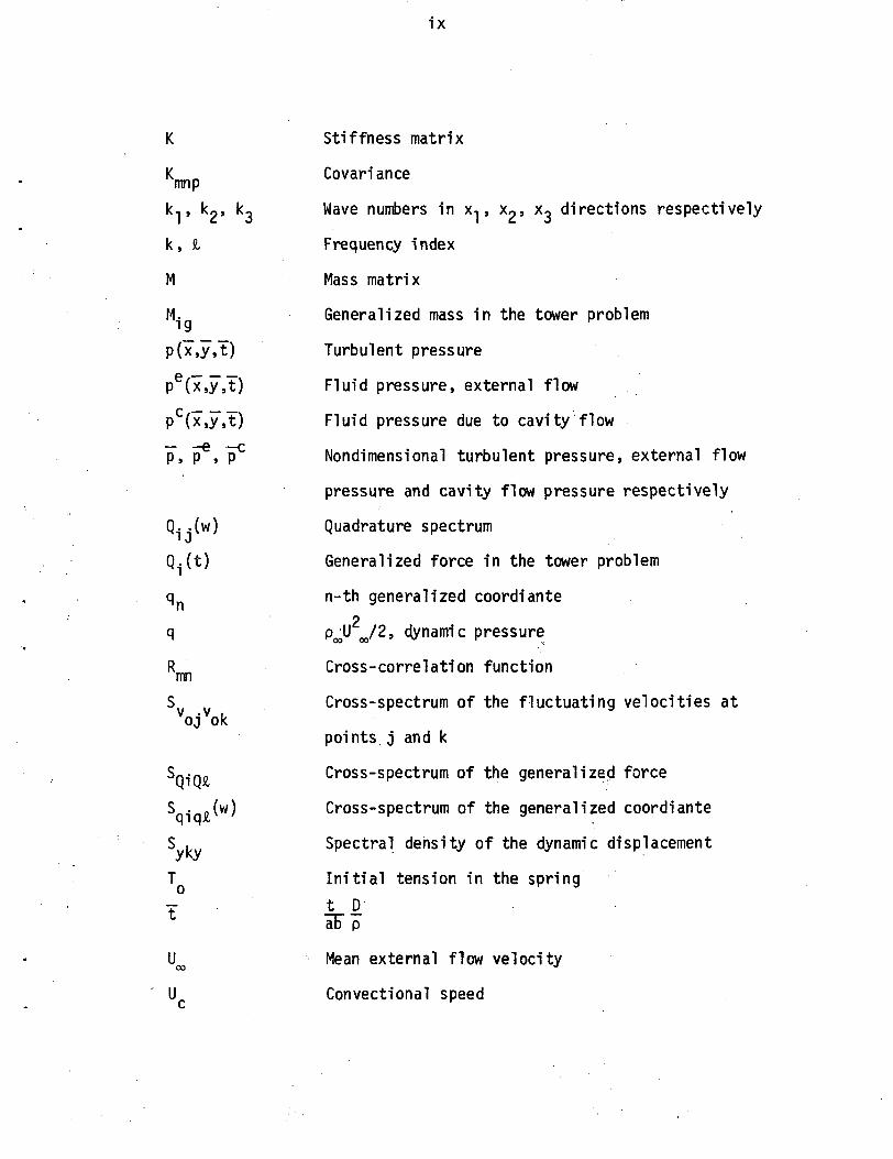
LIST OF SYMBOLS
A Displacement vector of the nth mode
a Velocity of sound for external flow00
a Velocity of sound for cavity flow
a (K), b (K) Time series amplitude coefficients
b.. Modal amplitude of plate vibration' J
C. . (w) Co-spectral density• J
D Plate stiffness
£[•] Expectation operator
F .(t) Dynamic wind load at the location j
F . Static wind load at the location jajF" Random generalized force for plate vibration
F6 f*mn' mn Aerodynamic generalized forces for external and
cavity flow respectively
F(t), T(t) Forcing function vector
f(x,t) Force per unit length of the strings\
f (x , t ) Nondimensional forcing function
f . j ( t ) Simulated time series
G(w) Spectral matrix
G (w) One-sided cross-spectral density
H (w) Element of lower triahgular matrix derived from
6(w)
vi 11
IX
K Stiffness matrix
K Covariance
k,, k2, k. Wave numbers in x-,, x^, x, directions respectively
k, S. Frequency index
M Mass matrix
M. Generalized mass in the tower problem
p(:x,y/t) Turbulent pressure
pe(:x,y,T) Fluid pressure, external flow
P (x,y,t) Fluid pressure due to cavity flow
p"» P^J P° Nondimensional turbulent pressure, external flow
pressure and cavity flow pressure respectively
Q. .(w) Quadrature spectrum
Q.(t ) Generalized force in the tower problem
q n-th generalized coordiante2
q p^U J2, dynamic pressure^
R Cross- correlation functionmnS Cross-spectrum of the fluctuating velocities at
oj okpoints j and k
Cross-spectrum of the generalized force
(w) Cross-spectrum of the generalized coordiante
S . Spectral density of the dynamic displacement
T Initial tension in the spring
t D
U^ Mean external flow velocity
U Convectional speed

•* Iutajt) Nondimensional displacement of the center of the
string
V . Mean wind velocity at the locationajV .(t) Pulsating velocity component
w Angular frequency
W Upper frequency cut-off
w. Lower frequency cut-off
w Nondimensional plate thickness
X_. • Elements of complex vectorPK
x", y, z" . Nondimensional co-ordinate
yk - Dynamic displacement
a (k) Phase angle
a • Modes of natural oscillation
3-|, $2 Damping coefficients
6 Logrithmic damping decrement of oscillation
Aw Frequency increments
c;pk Complex random number
?* Boundary layer thickness
v Poisson's ratio
£ , n Gaussian random variables
p Mass per unit length of the string
p Free stream density! OO
p Cavity flow density
R.M.S. of nondimensional response at the center
of the string

$ Airy stress function for membrane stress
$.(w) Transfer function in the tower problem
$, $c Velocity potential, external and cavity flows

CHAPTER I
INTRODUCTION
In this dissertation, two methods are described to simulate on a
digital computer a set of correlated, stationary and Gaussian time
series with zero mean from the given matrix of power spectral densi-
ties and cross-spectral densities. Some example problems are investi-
gated to show the power of this technique to solve the problems of
linear and in particular nonlinear random vibrations. The development
set forth is for any arbitrary number of correlated series; however,
in practice, the number is limited by the storage capability of the
computer.
The first method is based upon trigonometric series with random
amplitudes and deterministic phase angles. The random amplitudes are
generated by using a standard random number generator subroutine. An
example is presented which corresponds to three components of wind
velocities at two different spatial locations for a total of six
correlated time series. Selected spectral densities computed from the
simulated time series are compared to the original spectral densities
from which the time series were generated.
In the second method, the whole process is carried out using the
Fast Fourrier Transform approach in place of trigonometric series. It
is found that this method gives more accurate results and works about
twenty times faster for a set of six correlated time series.
1

To show one of the many areas of application of the present
method of simulation, namely the class of random structural vibration
analysis, the following problems have been investigated: (1) The
linear vibration characteristics of a long tower under the action of
correlated wind loads have been presented. Taking it to be a fourteen
degrees of freedom system, the time history of the displacement of the
top of the tower has been plotted considering up to three modes of
vibration. The usefulness of this method in the case of linear
analysis can be significant and very important, e.g., looking for the
occurrence of maximum structural response rather than the r.m.s. value
of response. This knowledge will be very useful for the reliability
study of structures under random loads; (2) One of the most interesting
and significant applications of the proposed method is the simulation
of random generalized forces. The necessity of simulating random
generalized forces arises when the dynamic response analysis is per-
formed in time domain either for the purpose of obtaining information
beyond the second order statistics (such as first passage time distri-
bution) or when the structure is nonlinear and therefore an approximate
random response is sought by simulating the excitation.
In order to assert the validity of the preceding discussion, the
problem of the nonlinear vibration ofa string has been solved in the
time domain by simulating the random generalized forces.
Finally to show the application of this method to a more complex
problem, the random nonlinear vibration of a flexible plate immersed
in a fluid flow on one side and backed by a fluid filled cavity of

finite dimensions on the other side is considered. The nonlinear
plate stiffness induced in the plate by out-of-plane bending and the
mutual interaction between the external and the internal fluid flow
is included.
The FFT simulation technique is utilized for the response
analysis of the plate undergoing large deformation. The same problem
has been done by Shinozuka [1] where he has taken a multidimensional
trigonometric series model for the generalized forces. The analysis
is performed in the time domain rather than in the frequency or wave
number domain as is usually done in linear response analysis. The
-numerical example has been presented for subsonic flow over the plate.

CHAPTER II
LITERATURE SURVEY
Part A: Review of Existing Simulation Methods
Numerous papers dealing with simulation of random process have
been published in recent years. Although many authors dealt with the
simulation of single random processes utilizing trigonometric series
[2], filtered white noise [2], filtered shot noise [3] and correlated
random pulse trains [4] etc, only Hoshiya and Tieleman [5], Shinozuka [6]
and Borgman [7] studied the simulation of multicorrelated processes.
I. In the simulation of ocean surface elevation, Borgman used wave
superposition by choosing the frequency in such a way that the ampli-
tude of each wave function was an equal portion of the cumulative
spectrum. Borgman also presented a method for simulating several
simultaneous time series by passing a white noise vector through
filters. He proposed the following model [7].
m °°y*(t) = A
m = 1, 2, ... M (2-1)
where,
ym(t) = m th time series

x.(t) = independent random inputs
= kernals
Let Smr(f) represent the cross spectral density between ym(t) and
yr(t). Kernals k (T) and its Fourier Transform T^A(f) are deter-
mined from the relation
rS t f\ _ y TT- / f\v t f\ c f f\
•mT"\^/ ~ " ^m-i V^/*^-»--i \^/^-,^-S \^/ •uij. ^J t I X i
j=i
r = 1, 2, ..., m and (2-2)
m = 1, 2 M
where the bar denotes the complex conjugate.
This system of equation can be solved sequentially (taking KJJ to
have zero gain for j = 1, 2, 3 ...) as
K2l(f) "/SJlTfT (2.3)
K22(f) = ES22(f) - |K21(f)|2]%tc.
This, in turn, determines the digital filter co-efficients, anmj,
needed to approximate the kernel associated with the system function
kmj(f). Then the final simulation equation reduces to
N Nym(kAt) = ^ ^ a^x., , k-n,
m = 1, 2, ... M (2-4)
in which x^, n for n = 1, 2, 3, ... is the j th generated sequence ofJ
independent, zero mean, unit variance, normal random variables.

II. Later Hoshiya and Tieleman [5] considered the following trigo-
nometric model for simulating two correlated random processes:
x(t) = E (a,-cos w.t + b.-sin w,-t)= J J J J
ny(t) = E (CCOS (Wt + a) + d-sin (Wt + a) (2-5)
where a,-, b-, c- and d- are random variables and Oj is deterministic.
The two stationary normal processes are correlated if there exists a
non-zero correlation between a,- and c,- and/or b,- and dn-. The co-J J J J
variance CXyj between the two random variables a^ and Cj is defined
as
cxyj = Etajcj] = EtbJdjl
and the standard deviation at frequency w- , axj and Oyj are given as
axj = (w-jMw (2-6)
ayj = ^(WjjAw (2-7)
where Sx(w,-) and Sy(wj) are the discrete form of the power spectra for
processes x and y respectively.
Expressions for the co-spectrum and the quadrature spectrum are given as
2CCy(Wj)Aw = axjayjpxy.jcos aj (2-8)
2QCy(Wj)Aw = -axjayjPxyjSin a-j (2-9)
whence,
and

The random variables a. and b^ are generated independently from aJ «
normal distribution with zero mean and a standard deviation
and Oyj = 2Sy(wj)Aw respectively. Then Cj and d:
are generated as follows. Since a< and c^ are both normally dis-J J
tributed, the joint probability density function of a^ and c* isF a-21 a;
.2
axj°yj
and.the probability density function of aj is
P(aj) =
The conditional probability density function of Cj for given 3j is
(2-iic)
Consequently, the conditional probability density function of Cj for
given aj is also Gaussian with mean Pxyj j and a standard deviation
i- Similarly, the conditional distribution of d- for a givenjand standard deviationb- is Gaussian with mean
xjThus random variable Cj is generated from Gaussian distribution with
mean Pxyj f9-; and a standard deviation of ayj 1-Pxyj' Similarly, thexj
random variable d- is generated from a Gaussian distribution with meanJ
i/ ?"and a standard deviation of a.,,- l - p -J Jj

8
III. In his paper [8], Shinozuka proposed a different
trigonometric model for the simulation of multivariate random pro-
cesses. He used a series of cosine functions with weighted ampli-
tudes, almost evenly spaced random frequencies and random phase
angles with uniform distribution. He considered a set of n sta-
tionary random processes fo.j(t) (i = 1, 2, ... n) with a specified
cross-spectral density matrix S°(w) = [S°f.f.(w)], where S°-p.f.(w)I J I J
are mean square spectral densities if 1= j and cross spectral
densities of fOj(t) and foj(t) if i 4= j.
He proposed the following model
x c o s [w j k t+ qjk + e^^)] (2-12)
where,
w^ (k = 1, 2, ... N) are random variables identically and independent-
ly distributed with the density function
gj(w) = iH-jjMlVj2 (2-13)oo
with a,2 = J |H in.(w)|2dw (2-14)J _oo JJ
and Q.. (k = 1, 2, ... N) are also identically and independently dis-
tributed with the uniform density l/(27r) between 0 and 27r. HJ.J(W)
are obtained from
Si.j(w) = Z. H1k(w)Hjk(w) (2-15)K~ I

and,
H^(w)(2-16)
(2-17)
The series simulated by the above technique have the asymptotic
ergodicity.
IV. Comparison of Various Approaches.
It appears that method of simulation proposed by Shinozuka [8] is
the most efficient so far. Thismodel [8] seems to be more general than
that due to Hoshiya and is more efficient than that due to Borgman [7].
Since the measured cross spectral densities are usually given
numerically in terms of the real and the imaginary parts or the
modulii and the angles, the computation work associated with finding
|H-jj(w)|, from which "YJJ(W) = |H1-j(w)|/Hj1-(w) and the angles 6-jj(w) .,
can be directly evaluated in the case of Ref. [8]. Therefore, method
of simulation presented here appears more practical than that proposed
in Ref. [7], which requires (a) the inverse Fourier Transformation of
N(N+l)/2 functions of w, H-J-J(W) and (b) the same number of integra-" <
tion in the time domain. Also, form of simulated functions con-
sisting of sum of cosine functions can be proved extremely advan-
tageous, when used as input, in evaluating the corresponding output
of a linear system.

10
PART B.
The main usefulness of the simulation method is in the area of
(a) a numerical analysis of dynamic response of non-linear structures,
(b) time domain analysis of linear structures under random excitations
performed for the purpose of obtaining the kind of information, such as
first excursion probability and exact time history of a sample
function, that is not obtainable from the standard frequency domain
analysis, and (c) numerical solution of stress wave propagation
through a random medium and eigen value problems of structures with
randomly non-homogeneous material properties. The usefulness of this
method has been demonstrated in the later chapter of this dissertation.
In this connection, it looks appropriate to make a relative study of
the prevalent methods of handling the non-linear random vibration
problems.
Review of Stationary Random Response of
Multidegree of Freedom Nonlinear Systems
Fokker-Planck Approach.
One exact method of studying the stationary random response of
a nonlinear system is the Fokker-Planck approach. If the excitation
is a Gaussian white noise, then the transitional probability density
of the response process is governed by the Fokker-Planck equation.
The equation governing the first probability density function for the
stationary response has been solved under the following rather
restrictive conditions:

11
(1) the damping force is proportional to the velocity
(2) the excitation is a Gaussian white noise
(3) the correlation function matrix of the excitation is
proportional to the damping matrix of the system. Under the above
conditions, the equation of motion may be written as follows:
(2-18)MX + Cx + = f(t)3x
= 0
with
= 2YC6(T) (2-19a)
where y is a constant, u(x) is the potential energy of the system and
/ 3u \
(2-19b)3.xl
3'u3x«
\Suppose that there exists an orthogonal matrix A which can simul-
taneously diagonalize the mass matrix M and the damping matrix C:
(2-20)
where V and A are two diagonal matrices. Then, upon using the trans-
formation x = Az and noting that
" ' 3u(I)jj=l J'm J>< 3zk
m = 1 , . . . n
3X3u(
3X 3z
_ 3u(z
3z(2-21)

12
Equation (2-18) becomes
Vz + AZ + j = ATf(t) = b(t) (2-22a)
and the correlation function matrix of b~(t) is given by
R^T) = 2YAS(T) . (2-22b)
The stationary Fokker Planck equation associated with (2-22a) is given
by
(2-23,
where A- and v- denote the j th diagonal element of A and V, p is thei
abbreviation for the first probability density of the Markovian/z\
vectorf^J. The solution to (2-23) may be written as follows:
p(z,z) = 3 expj-^E VjZ.,.2 + u(I)]J. (2-24)
This solution was first obtained by Ariarathan [9] for a two-degree-
of freedom system, and it was extended to the above form by Caughey
[10]. The constant 3 in (2-24) is a normalizing factor such that
r f°°••• j p(F iz)dz1...dzndz1...dzn = 1- (2-25)
-«
In the original co-ordinates, equation (2-24) becomes
p(x,x) = B exp« - 7|9x'Mx + ufx) >. (2-26)I l V
It will be noted that the terms in the square brackets are
respectively the kinetic energy and the potential energy of the system.

13
Equation (2-26) may also be written as
p(x,x) = B exp {--gi xMTx> exp {- lu(x)> (2-27)
Hence x" and x~ are linearly independent.
Normal Mode Approach
Consider an n-degree-of-freedom system governed by the equation
of motion
MX + C^x" + K(°)X + y?(x,x) = f(t), (2-28)
u = a small parameter
The matrices c'°).. and K*0' are respectively the damping matrix and
the stiffness matrix of the system due to the linear part of the•
damping forces and the spring forces, and yc (x,x~) represents the non-
linear forces of the system. Here, T(t) is a stationary Gaussian random
vector. Without loss of generality, one can assume that the mean vector
of T my = 0.
In using this approach, the following two conditions must be
satisfied: (1) the linear system obtained by neglecting the nonlinear
term g"(x~,x~) in (2-28) must possess normal modes; (2) the correlation,
function matrix R^T) must be diagonalized by the same matrix which
diagonalizes the matrices M, C*°' and IO°^.
The second condition is quite restrictive and is seldom realized in
real systems.
Assume that the above restriction can be met, then there exists
a matrix A such that

14
ATMA = I
= wk(o)5ki
* KJ (2-29}( *
ATRf(t)A = D(T), dkj = dk(T)6kj.
By using the transformation x~ = Az~, Eq. (2-28) reduces to
z + A(o)t + n(o)I + yATg(z,I) = ATf(r) = F(t) (2-30a)
Where the correlation function matrix of b is
MT) = D(T) . (2-305)
In component form Eq. (2-30a) becomes
.. . - j » z ) = bj(t) (2-31a)K~" I
and Eq. (2-30b) becomes
E[bk(t)b.j(t+T)] = dk(T)6k.j, j, k = 1, ... n. (2-31b)
The differential equation in (2-31 a) may be written as
' j = 1 , ... n
where the deficiency term e..- is given by
._ _+ y E akjgk(z,z), j = 1, ... n (2-33)
K*~ I
2If the quantities Xj and Wj are chosen in such a way that some
measure of the deficiency term is minimized, then it seems reasonable
that the statistics of the response of the nonlinear system can be
approximated by those of the linear system described by
Zj + XjZj + Wj2Zj = bj(t), j = 1, ... n (2-34)

15
At this stage, the differential equations are uncoupled and the
excitation b(t) is an uncorrelated vector process. Hence each un-
coupled differential equation can be solved separately.p
In order to determine Xj and Wj , Caughey [11] chose them so as
to minimize the mean square value of the deficiency term e. This can
be achieved by requiring that
] = 0 \1\j = 1, ... n. (2-35)
f?1?] = 0'
Substituting (2-33) in (2-35) and interchanging the order of dif-
ferentiation and expectation, we obtain
~" I
= (Wj(o))2 + u Z akjt[z.jE[z.jgI<(z",z)] (2-36)l\~" I
W;
Equations (2-34) and (2-36) can be used to find various mean square
values of the response process.
In certain cases, the contribution from the first mode may be
dominant. In these cases, we may let x. = a^-iz-i in the aboveJ w
derivation. Then
n
3=1 (2-37)n n . 9
XT = X^ + y Z a. j lE[z1g..(z1,z1)]/Etz1^].J "~ *

16
This is rather a rough approximation, but it is very simple and in some
cases, it does give reasonably approximate solutions.
Perturbation Approach
Consider the same problem as defined in the previous section, whose
equations of motion are
MX + G(°)X" + K ^ ° % + yg"(x",x) = ?(t) (2-38)
Assume that y is so small that the solution of Eq. (2-38) can be
approximately represented by [12]
x" = Xg + yx"-j (2-39)2
Substi tut ing (2-39) into (2-38), neglecting terms involv ing y,n 0 1y3, ... and equating corresponding coefficients of y and y yields
the following sets of linear differential equations:
Mx0 + C(°)x0 + K
(°)x0 = f(t) (2-40a)
MXT + C(°)x-, + K(°)X-, = -g"(x0(t),x0(t)) (2-40b)
Correct to the same order of accuracy, the instantaneous correlation
matrix for displacement becomes
E[xxT] = E[x0x0T] + y{E[x071
T] + E^Xg1]}- (2-41)
Note that
E[XOX-|T]= (EtXoX-,1])1. (2-42)
The matrix E[XQXQ] can be found from (2-40a) by the various approaches
as in linear analysis, and EJ'XQX' ] may be evaluated as follows.
Since (2-40a) and (2-40b) are linear, their stationary solutions are
XQ = J G(t-T)f ( i )dT (2-43a)

17
dT , (2-43b)
where G(t) is the common impulse response function matrix of (2-40a)
and (2-40b) and g(x) is the abbreviation of (XQ(T) ,XO(T)). Thus,
E[XOX.,T] = - f f G(t-T1)E[f(T1)g
T(T2)]
x GT(t-T2)dT1dT2 . (2-44)
The matrix E[?(T| )gT(T2)] can be evaluated with the help of proper-
ties of Gaussian processes. Therefore, we can find E ^ g x ] and
hence E[xxT].
Usual ly , the evaluation of the integrals in (2-44) is not easy, so
Tung [13] has developed a different approach to generate E[xxT]
from (2-40a) and (2-40b). He applies Foss's method [14] to uncouple
(2-40a) and (2-40b) into first order differential equations and then
solves the resulting equations to f ind the various instantaneous
correlation matrices.
This approach wi l l fail if the damping matrix f/°^ is a nul l
matrix. In this case, Equation (2-40a) does not have a stationary
solution since all its correlation functions w i l l f ina l ly go to
inf ini ty . Another l imitation of this approach is that not onlymust the
nonlinearity of the system has to be small , but also the excitation
has to be suff icient ly low.
Generalized Equivalent Linearization
The normal mode approach is qui te powerful if it applies. How-
ever, due to the conditions imposed on the excitation, its appl icat ion

18
is rather limited.
In his thesis Yang [15] introduced a more general approach.
Except that the excitation must be stationary, the only additional
restriction to this approach is thatthe excitation be Gaussian. In
this approach, we define an auxiliary set of linear differential
equations for the original nonlinear system. The solution of the
original nonlinear system is approximated by the solution of an
auxiliary set and the unknown co-efficients are chosen in such a way
that some measure of the difference between the two sets of equations
is a minimum.
Consider the following linear equation
MX + Cx~ + Kx = ?(t) (2-45)
and the nonlinear system given by
fft + g(x,x~) = f(t). (2-46)
The difference between (2-46) and (2-45)
e~= g(x~,x) - ex" - Kx" (2-47)
The necessary conditions to minimize E.[e~e] are given by
SE[?Te] = 2E[eT 3ef 1 = 2E[e,x.] = 0
ik_ _ ^ (2"48)
3E_[eJ_e]_= 2E[eT e ] = 2E[e.x,] = 0-3k-,. I 3k i k J J
J ix J IV
Upon using Eq. (2-47), they become in the matrix form
E[exT] = Etg^x.xlx"1] - E[xxT] - KE[xxT] = 0
_T _^-,-T .*-T —TE[ex ' ] = E[g(x,xlx'] - CE[xx ' ] - KE[xx ' ] = 0
It has been shown that the conditions in Eq. (2-49) do define a
minimum for E[e~Te"][15].

19
In order to solve Eq. (2-49) for K and C, it is first necessary to_ JL __ .T __ : __ J.T __ T _ I.T
express E[g(x,x)x ' ] and E[g(x,x)x ] in terms of E [xx ' ] , E [xx ' ] and
E[xx~T]. Let ykr denote the displacement of k th mass relative to
the r th mass and let the approximate force acting on the k th mass
by the nonlinear element connecting the k th mass and the r th mass
be denoted by Skr(ykr»ykr) . Then• •' •
E[gk(x",x),x.j] = z E[Skr(ykr,ykr)x.j]
r4k (2-50)
E[g k(x>x)x j ] = z
where the sum is taken over all nonlinear elements connected to the
k th mass. Since x~ is a Gaussian vector, it follows that the• •
quantities ykr, y. , x-> and Xj will be Gaussian distributed. Hence
E[Skr(ykr,y|<r)xj] = E[Skr(ykr,ykr)ykr]
E[Skr(ykr,ykr)x.j] = E[Skr(ykr,ykr)ykrl
x E[ykrx..]/E[y r]
Define
Ykr = E[Skr(ykr,ykr)ykr]/E[yk2]xkr = E[Skr(ykr,ykr)ykr]/E[yk2]
Then Eq. (2-51) reduces to
E[Skr(ykr.Ykr)Kj] = r "-"".J- (2.53)E[Skr(ykr,ykr)x..] = E[(Ykrykr *

20
Hence, there exists a linear system with spring constant X^ and
damping co-efficient y^ defined by Eq. (2-52) such that if the
nonlinear system is replaced by this linear system, the expectation_ ^ . .— _ • • -p
values E[g(x,x")x ' ] and E[g(x,JOx ] will not be changed.
Substituting Eq. (2-53) in Eq. (2-50) gives
E[gk-(x,x)x.,] = E[l(Ykrykr
_ _ . . (2-54)E[gk(x,x)x.,] = E[Z(Y|<rykr + Xkrykr)xj]
Let the stiffness matrix and the damping matrix of the linear system
defined by Eq. (2-52) be denoted by K^e) and C^. Then Eq. (2-54)
can also be written as
(2-55)
E[gk(x,x)x.,] = E[j i(CJe)xs + KJe)xs)Xj]
since the right-hand side of (2-54) and (2-55) are just two different
representations of the total force acting on the k th mass. In
matrix form Eq. (2-55) becomes
E[g"(x,x)xT] = c(e)E[xx"T] + K
E[g"(x,x)x"T] = c ~ "
Substituting Eq. (2-56) in Eq. (2-49) and solving for K and C whichT. .
minimizes E[e e], yields
(K - K^bEIxx"1] + (C - C ( e))E[xx~T ] = 0 /
(K - K ( e))E[xxT] + (C - C ( e ) )E[xxT ] = 0

21
which can also be written as
E[xxT] E[xxT]
E[xxT] E[xxT]
( K -
(C -= 0. (2-58)
If the square matrix is non-singular, the only solution to Eq. (2-58)
is
K =(2-59)
If the square matrix is singular, (2-59) is not the only solution.
But in this case any solution to Eq. (2-58) will lead to the same
minimum for E[ee']. So we still can use Eq. (2-59).
Thus, it has been shown that the linear system formed by
replacing each nonlinear element by a linear spring and a linear
damper defined by Eq. (2-52) will minimize E[ee~T] provided that the
excitation is Gaussian.
It should be pointed out that the smallness of the nonlinear
term in the original equation was not a presupposition in the develop-
ment of the above method. In general, the accuracy of this method
depends on the smallness of the nonlinearity. When the nonlinear
terms are not small, this method is often an iterative procedure.
This concludes the relevant literature survey. In the light
of the review study in this chapter, we will be better able to
appreciate, in the next chapters, the power and usefulness of the
simulation approach in the analysis of random linear and nonlinear
problems.

CHAPTER III
DISCUSSION OF SIMULATION METHODS
In this chapter we will present two methods to simulate a set
of Gaussian processes (f-|(t), f2(t), ... fm(t), ... f (t)} when the
power spectral density function of each process and cross spectral
density functions between any two processes are known. These
spectral densities are usually arranged in the form of a matrix
commonly known as spectral matrix. This matrix is given by
G12(w) ... G1M(w)
G(w) =G21(w) G22(w) ... G2M(w)
GM](w) GM2^W) •••
(3-1)
where Gmn(w) is the one-sided cross spectral density between the pro-
cess fm(t) and fn(t). When m + n, Gfnn(w) is complex with real part
Cm^w) called the co-spectrum and imaginary part - Qmnlw) called the
quad^spectrum. When m = n, the quad-spectrum is zero and then
Gf^w) stands for power spectrum for that particular process.
I. Trigonometric Model
Here we will show that a set of random processes can be simu-
lated by a trigonometric series of the form
N= z {ai l(k)cos [wkt + on(k)]
K~ I
+ bn(k)s1n [wkt + an(k)]>(3-2a)
22

23
Nf2(t) = Z {a21(k)cos [wkt + o21(k)] + b21(k)sin [wkt + a21(k)]
K I
+ {a22(k)cos [wkt + a22(k)] + b22(k)sin [wj^t + a22(k)]>
(3-2b)
fm(t)=k^
{aml(k)cos [V + <W<>] + bml<k>s1n
am2(k)cos [wkt + (^(k)] + ^(kjsln [wkt
More generally, the above set of processes can be represented as
m Nfm(t) = Z Z {amp(k)cos .[wkt t -anptk)]
p~" I K~~ I
+ bmp(k)sin [wkt + o p(k)]. (3-3)
The coefficients amp(k) and bmp(k) are Gaussian random variables with
zero mean that have the following additional properties: (i) amp(k)
and bnq(2,) are always independent and for the case when m = n, p = q
and k = 1 they are identically distributed, (ii) amp(k) and anqU)
(or t>mp(k) and bnq(S,)) are statistically correlated if p = q and
k = a, otherwise they are independent.
The phase angles (k) are deterministic. Since the co-
efficients amp(k) and bnq(k) are Gaussian distributed it follows from

24
the Central Limit Theorem that the time series fm(t) will also be
Gaussian distributed.
The form of the simulated time series given by Eq. (3-3) lends
itself to a very simple physical interpretation. For the first time
series (m = 1) the index of summation p takes the value of unity.
For the second time series (m = 2) the index p takes the values
unity and two. The value of p = 2 adds to the second series two
terms that are independent of the first series. Physically it adds
some energy to the second process independent of the first process.
Likewise for each new process two additional terms are tacked on which
allow that process to have some energy that is independent of all the
previous processes.
In order to see how the co-efficients amp(k) and bn (£), and
the phase angles amp(k) should be determined it is necessary to con-
sider the cross correlation between the time series fm(t) and fn(t).
Here for convenience we will assume m £ n. The cross correlation
between these time series is given by
R^T) = E[fm(t)fn(t +T)]
m n N N= E[ Z Z Z Z
p=l q=l k=l £=1
{amp(k)anqU)cos [wkt + ^(kjjcos [w£(t + T) + an
+ amp(k)bnqU)cos [wkt + ^(kjlsin [wA(t + T) + o
+ bmp(k)bnq(A)sin [wkt + amp(k)]sin [w£(t + T) + anq(£)]>]
(3-4)

25
The expectation operator can be brought inside the summations,
and since the expectation of a sum is the sum of the expectations, we
get
m n N NR^T) = Z E E E
p=l q=1 k=l A=l
{E[amp(k)anq(£)]cos [wkt + o^pfkj jcos [wk(t + T) + anqU)]
+ E[amp(k)bnqU)]cos [wkt + amp(k)]sin [wA(t + T) + anqU)l
+ E[bmp(k)anqU)]sin [wkt + amp(k)]cos [w£(t + T) + anqU)]
+ EtbmpCkJbnqf^Jls in [wkt + ^(kJlsin [w£(t.+ T) + anq(£)]}
(3-5)
Because amp(k) and bnq()l) are always independent the middle terms in
the above expression are both zero. Furthermore, since amp(k) and
anq(^) (°r bmp(k) and bnq^^ are independent unless p = q and k = £,
Eq. (3-5) reduces to
m N
{E[amp(k)anp(k)]cos [wkt + cxmp(k)]cos [wk(t + r)
+ E[brnp(k)bnp(k)]sin [wkt + (%p(k)]sin [wk(t + T) + anp(k)]}
(3-6)LetKmnp(k^ = Etamp(k)anp(l<)]. That isK f f lnp(k) is the covariance
between amp(k) and anp(k). Because b^pfk) has the same distribution
as amp(k), we also have K^p (k) = E[bmp(k)bnp(k)] . Using these
relationships and a trigonometric identity Eq. (3-6) becomes
m N) = E E K^pdOcos [wkr - ofTlp(k) + anp(k)] (3-7)
p=l k=l

26
The right hand side of Eq. (3-7) is independent of the time t; there-
fore, the assumed trigonometric form for the time series yields
stationary random processes.
Noting the fact that the spectral density is the Fourier Trans-
form of the correlation function, the one-sided cross-spectral
density for processes fm(t) and fn(t) is given by
2 j" l\nn(T)iJWTdT, w> 0(3-8)
0, w < 0
The next step is to substitute Eq. (3-7) into Eq. (3-8) and perform
the integration. However, it should be recalled that KmnpCO in Eq.
(3-7) is the expected value of amp(k) times anp(k) (or bmp(k) times
bnp(k))- Therefore, by substituting Eq. (3-7) into Eq. (3-8) what
we obtain is an expected value for the cross-spectral density. Thus
we have
m N2 Z Z
r ,-JWTx I cos [wkx - omp(k) + anp(k)]e di}
w > 0
(3-9)0, w < 0
Carrying out the integration gives
m N2ir Z Z Kj^p^Mw - wk)
E [ G m n ( w ) ] = 1 P=1 k=1
x {cos [Ofpptk) - anp(k)] - j sin[ofop(k) - anp(k)]} , w _> 0
Q, w < 0 (3-10)
where 6(w - w^) is the Dirac delta function.

27
We thus see that for the assumed trigonometric time series given by
Eq. (3-3) Gftn is composed of both real and imaginary terms. When
m = n, Gjnn corresponds to a power spectral density and the imaginary
portion is zero. A schematic plot of Eq. (3-10) is shown in Figure
1. The frequencies w^ are chosen such that
wk = w£ + (k - ^.)Aw, k = 1, 2, ... N
Aw = Wu " w* (3-11)N
where wu and w,, are respectively the upper and lower cut off fre-
quencies of the spectra that is used to generate the time series.
Suppose an actual power spectrum G(w) for which we want to obtain a
simulated time series is shown in Figure 2. We can slice this
spectrum up into N intervals of width Aw as shown. The amount of
energy contained in the slice centered at w = W|< is Gfw^Aw. We want
the expected value of the spectrum corresponding to our simulated
time series to have the same amount of energy at w = w^. This means
that the expected amplitude of the delta function at w = w|< should be
G(w)Aw. Similar criteria must be applied for the cross-spectra of the
simulated time series.
We assume that at any frequency w = W|< the cross-spectral
matrix can be factored into an upper and lower triangular matrix,
where the upper triangular matrix is the complex transpose of the
lower triangular matrix, as indicated below:

28
'mmt
t t 1 I J1
W, W2 Wk WN
w, wu
w
Fig. 1 . Schematic sketch of a discrete power spectrumfrom a simulated time series.

29
'mm
" W, WoW,
W
AW
Fig. 2. Schematic sketch of a continuous power spectrumused to generate a time series

30
Gn(wk) G12(wk)
G21(wk) G22(wk)
. G l M (w k f j
. G2M(wk)
GMl(wk) GM2(wk) GMM(wk)
Hn(wk) 0 ... 0
H21(wk) H22(wk) ... 0
Hm(wk) HM2(wk)
Hn(wk) H21(wk) ... HM1(wk)
0 PT22(wk) ... HM2(wk)
0 0 HM M(w k)
( - 1 2 )
The bar is used to denote the complex conjugate.
If Eq. (3-12) holds then
Ww) = Z VW)VW) (3-13)
for n <_ m. Eq. (3-13) can be rewritten with the limit of summation
taken as m instead of n since Hmn(w) = 0 for m > n. Thus Eq. (3-13)
becomes
m _W"> - z Hmp(w)Hnp(w) (
P=l
Using the above relation,solutions are obtained as
where [fo(wk) is the m th principal minor of G(wk) with D0 being
defined as unity, and

31
H (w, } = H (wi ) 6(1, 2, , p - 1 , .m\"nipple' Hpp^wk; vl 2, p - 1. V,
D k ( w ) ( 3 - 1 6 )
.p = 1, 2 M, m = p + 1 M
where,
"11 6-10 G-i , I Gln
G/l, 2, ..., p-1, m\M, 2, ..., p-1, p;
321
Gp-l,l, GP-1,2 ' ' ' ' Gp-l,p-l GP-1,P
Gml > GmZ ' • • • • • ' jp-l ^p
is the determinant of a s'ubmatrix obtained by deleting all elements
except (1, 2, ... p-1, m) th rows and (1, 2, ... p-1, p) th columns of
G(wk).
It is noted that the above solutions are valid only when the matrix
G(w) is Hermitian and positive definite, as can be seen from Eq.
(3-15).
Because the cross-spectral density matrix G(w) is known to be only
non-negative definite, special consideration is needed in those cases
where G(w) has a zero principal minor. This is discussed in Appendix
C.
For the band of frequency [WL - -^ Aw, wu + rAw] we want the ex-l\ ^ "• C.
pected value of the energy in the spectrum of the simulated time
series to be equal to the energy Gmn(w)Aw of the original spectrum.
Thus equating the energy in the band centered at w = wk as given by
Eqs. (3-10) and (3-14) we get
2TrKnlnp(k){cos [Ompfk) - o^k)] - j sin [^(k) - o^k)]}
= Hmp(wk)Hnp(wk)Aw (3-17)

32
If we write
(3-18a)
(3-18b)
= RE[Hmp(wk)] + 3 IM[Hmp(wk)] (3-18c)
then by substituting Eq. (3-18a) into Eq. (3-17) we can see that
= lHmp(wk)ltcos sin
From Eqs. (3-18b) and (3-18c) we find
-1 IM[Hmp(wk)](3-20)RE[Hmp(wk)]
Thus it follows, as stated earlier, that the phase angles are deter-
ministic.
We recall that
(3-21a)
(3-21b)
That is we want amp(k) and bmp(k) to be independent random variables
with their covariances given by the right hand side of Eq. (3-19).
This can be done in the following manner, if we let
E[amp(k)a (k)]or
E[bmp(k)bnp(k)]
and
(3-22a)
(3-22b)
where m = 1, 2 M; p = m, m + 1, ... M and f and n are in-
dependent Gaussian random variables generated on a digital computer.
Because the £'s and n's are Gaussian distributed, the a's and b's
will also be Gaussian distributed.

33
Substituting Eq. (3-22a) in Eq. (3-21a) or Eq. (3-22b) in Eq. (3-21b)
and taking the expectation of both sides we see that in order to
make the left-hand-side equal to right-hand-side, the mean of £ or
n should be zero and their variances should be unity.
From Eq. (3-21 a) we have
and
(3-23b)
Thus the terms amp(k) (or bmp(k)) satisfy the properties stated earlier
and they also satisfy Eq. (3-17).
This concludes our explanation of how to simulate several multi-
correlated time series.
After discussing the Fast Fourier Transform in the next section, we
will give an example problem to check and compare the two methods.
II. Fast Fourier Transform (FFT) Method
Assume that a set of discrete time series can be represented by the
following expression:
fpn ' JT SXPkEXP(J T1] (
where ,
p = number of time seriesn = time indexk = frequency index
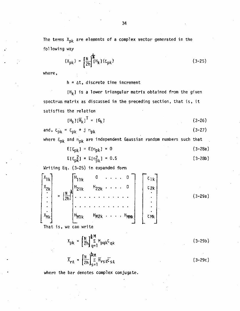
34
The terms Xpk are elements of a complex vector generated in the
following way
{Xpk> = f?h1*HkHCpk> (3-25)
where,
h = At, discrete time increment
[Hk] is a lower triangular matrix obtained from the given
spectrum matrix as discussed in the preceding section, that is, it
satisfies the relation
[Hk][Hk]T = [6k]
and, ?pk = spk.+ j npk
(3-26)
(3-27)
where £ni. and nnk are independent Gaussian random numbers such that-pk
E[Cpk] = E[npk] = 0
E[^J = E[n2k] = 0.5
Writing Eq. (3-25) in expanded form
(3-28a)
(3-28b)
lk2k
Mk
N_ik2h
H]lk 0 . . . . 0
H21k H22k ' ' ' ' °
HMlk HM2k • • H MMk
C2k
CMk
(3-29a)
That is, we can write
pk = [aDiH (3-29b)
(3-29c)
where the bar denotes complex conjugate.

35
Then,
V i - " cr<Xr*,] " 2h E[
N M M
Moving the expectation operator inside, we can write
<3-30b)
Making use of properties of complex random number as given in terms
of £'s and n's by Eqs. (3-28a) and (3-28b), it can be easily seen
that
where 6qs and S^ are Kronecker delta functions;substituting (3-30c)
into (3-30b), we get
M M My T H H (S & f^-^la^
q=l s=l
M(3-31b)
Taking the inverse Fourier Transform of Eq. (3-24), we get
X,nk = SPk n=0 r"
Therefore,
xp(N-k) = ^
N-l(3-32b)
n=0 r"

36
Since f is real, comparing Eqs. (3-32a) and (3-32b), we see
that
Xp(N-k) = xpk (3'33)
Thus, it is only necessary to generate Rvalues of X for each time
series because the other half of the values of X are just the complex
conjugate of the first half of the values of X.
Now, it is necessary to show that time series represented by
Eq. (3-24) do indeed have the proper power and cross-spectral
densities.
From Eq. (3-24)
Since f is real, taking the complex conjugate on both sides of
the above equation, we can write
Thus, the cross correlation between time series p and time series r
is given by
Rpr(n,m) = Etfpnf^] (3-34a)
where, n and m stand for the time indices of process p and process r
respectively.
Substituting for fpn and f^ from Eq. (3-24) and Eq. (3-24a)
respective7y in Eq. (3-34a), we get
R p r (n ,m) = E[Jj-2 I I XpkX r J lEXP[j MjpM-jj (3.34b)

37
Moving the expectation sign inside
1 N-l N-l
k=0 &=0
x EXP[j N " — ] • (3-34c)
From Eq. (3-31b)one obtains
- _ N M
q=l
Substituting this in Eq. (3-34c)
-, N-l N-l MRpr(n,m) = " - - - . . - - ^
x Exp[j i]. (3_34d)
Unless k = H, Eq. (3-34d) is zero.
Hence,
Rpr(n,m) = H"''" -) • (3-34e)
That is, the correlation is a function of the time lag which
proves that the process is stationary.
Finally we can write Eq. (3-34e) as
The spectral density function is the inverse Fourier Transform of
Eq. (3-35). That is
6prk = 2h "Vllprdn-iOEXPM Mtol] (3-36a)K~U
- S Hpqkff k (3-36b)q=l

38
which is equal to the elements of the spectral matrix between the
process p and process q.
Thus, we see that the assumed form of the time series given by
Eq. (3-24) has the same spectral density as the target spectral
density function.
Simulation of Strong Wind Turbulence
In order to check the two simulation techniques described above
namely the trigonometric model and Fast Fourier Transform model, we
generated six correlated time series representing the fluctuating
part of wind velocities. These six series represent the three com-
ponents of the wind at two different spatial locations. Each simu-
lation technique was checked by comparing the spectra of the simulated
data to the spectra used to generate the data. The input spectra
used for these time series are based on wind velocity measurements
made by several investigators [16, 17, 18]. These spectra will not
be discussed here in detail. Under strong wind conditions turbulence
is due to mechanical mixing caused by fractional effects. In this
case, the turbulence can be considered a stationary random process with
zero mean and a Gaussian distribution.
The following expressions for the spectra were used for this
simulation:
u* ((1.0+1.5 (ig.
nC22(n) _ __2
u*2 ((1.0 + 1.5 (7.368f1)°'781)2.134

39
nC33(n) 3.36f]
u*? " 1 + 10f,5/3 ^
nC4 4(n)_ 272.2f2 _ _ _ _ _ ( j_4o)
U*2
nC55(n) _ 46.46f2
u*2 ((1.0 + 1.5 (11.06f2)°-781)2-1
, 3.36f2
u*2 1 + 10f25/3
nCl3(n) _ 12.(3-43)
u*2 (1.0 + 7.5f!)8/3
nC46(n) _ 12.5f2
u*2 (1.0 + 7.5f2)8/3
C]4(n) = (C11(n)C44(n))}5(exp(-19Af))}scos (2irAf) (3-45)
Ql4(n) = (C11(n)C44(n))Js(exp(-19Af))35sin-(2TrAf) (3-46)
C25(n) = (C22(n)C55(n))}2(exp(-13Af)^cos (4irAf) (3-47)
Q25(n) = (C22(n)C55(n))^(exp(-13Af))}5sin (47tAf) (3-48)
C36(n) = (C33(n)C66(n))J2(exp(-13Af)^cos (4irAf) (3-49)
^36^) = (C33(n)C66(n))Js(exp(-13Af))3Ss1n (4irAf) (3-50)
C34(n) = (C13(n)C46(n))^(exp(-16Af))^cos (3irAf) (3-51)
C16 = C34 (3-52)
Q34(n) = (C13(n)C46(n)')Js(exp(-16Af))J5s1n (3rrAf) (3-53)
Q16(n) = Q34(n) (3-54)
where C^ and Q^j represent the co-spectrum and quadrature-spectrum
parts of the spectral density function respectively.

40
Note that C^ = Cj^
and Qfj --Q-n
The elements of the components of the spectral matrix, which have not .
been listed above, have been assumed to be zero. The following actual
values were used for simulation
z1 = 100 ft, z2 = 50 ft
v-| = 60 ft/sec., V2 = 50.974 ft/sec.
f-| = nz-]/v-|, f2 = nz2/v2
u*2= (5.212)2 = 27.1649 ft2/sec2
f = nAz/7 = n (100 - 50)/(60.0 + 50.974)/2
where 7= average velocity
n = frequency in cycles per sec.
Suffix 1 or 2 refers to the station at 100 ft or 50 ft respectively.
Results
Fig. 3-a shows a set of six simulated correlated time series
based on the trigonometric model. Time series one, two and three repre-
sent the wind velocities in the mean wind, cross wind and vertical
direction respectively at a height of 100 ft. Time series four,
five and six are similar simulations for a spatial position 50 ft.
below the first point. Series one and four are positively correlated,
while series three and six are negatively correlated to one and four.
Series two and five, the series representing the cross wind, are
positively correlated to each other but uncorrelated to the other
four series. For these series, velocities were calculated every second

41
for 2048 seconds. The number of frequencies used, equal to N in
the analysis, was 600.
Fig. 3-b shows a similar set of simulated time series based on
the Fast Fourier Transform method. It is interesting to note the
similarity of the outcome. The number of frequencies used, equal
to N in the analysis, has to be the same as the number of time points
that is 2048.
A comparison between the spectra used to generate the simulated
data and the spectra of the simulated data is presented in Figures
4-a through 9-a for the trigonometric model and in Figures 4-b
through 9-b for the FFT model. Figures 8-a and 9-a are respectively
the co- and quad-spectra between time series one and time series four
based on trigonometric model. Figures 8-b and 9-b are the FFT counter
part. In each case the solid line represents the original spectrum
and the dashed line represents the spectrum of the simulated time
series. The spectra were calculated from the simulated data using
the "Cooley-Tukey" method of calculating the correlation function
first, and then the "Tukey window" was used for smoothing purposes.
As can be seen the comparison between the actual spectra and the
simulated spectra is quite good in all cases. We did not consider it
necessary to show all 36 possible power and cross-spectra. The
agreement looks the worst for the quad-spectrum between series one
and four (Figures 9-a and 9-b). The vertical scale for this compari-
son, however, is very expanded and about all we can conclude is that
both the original and simulated spectra are very close to zero. Also,

42
00
•^ o
uT op
I:\£* o?
00
o
*' i \ «"•' *' JM/f'tv'I'11 • i1 ME»y < 11 '•'*$t< I ''t'1! iM ,u .v **?"\ if
' ' / .' I
FIG 3A. SIAJLATED WIND VELOOTES BYTRIGONOMETRIC MODEL
THE TOTAL RECORD LENGTH IS 2048 SECONDS

43
ft 00
o
00
%H> wA|
FIG 3B. SIMULATED WIND VELOCITIES BYFFT METHOD
THE TOTAL RECORD LENGTH IS 2048 SECONDS

44
.00 L 08I
2 51 3 It
Fig. 4a. Comparison between the original G-|](w) and the spectrumof the first simulated time series based ontrigonometric model. (Vert. Scale: 100(M2/sec)/in;Horz. Scale: 0.53(rad/sec)/in)

Hci _
45
Oao'
. S3 2W
Fig 4b. Comparison betwejen the original G-j- |(w) and thespectrum of the first simulated time series basedon FFT model. (Vert. Scale: 100(M2/sec )/1n;Horz. Scale: 0.63(rad/sec)/in)

46
8
8R
.00 1 88 Z 51
Fig. 5a. Comparison between the original G22(w) and the spectrumof the second simulated time series based ontrigonometric model. (Vert. Scale: (50 M2)/sec)/in;Horz. Scale: 0.63(rad/sec)/in)

47
clQ--t"
ub
a/•-i
c. 00 1 25
Wi 83 51 3 L4
Fig. 5b. Comparison between the original GWw) and thespectrum of the second simulated time series basedon FFT model. (Vert. Scale: (50M2/sec)/in; Horz.Scale: 0.63(rad/sec)/in)

3F
8
48
8d.
enLJ
8in'
oao.00 L 25w Z SI 3 LI
Fig. 6a. Comparison between the original G^w) and thespectrum of the third simulated time series basedon trigonometric model. (Vert. Scale: (5 M^/sec)/in;Horz. Scale: 0.63(rad/sec)/in)

49
mu
63 I 25W
i 8S 2 51
Fig. 6b. Comparison between the original 633 ) and thespectrum of the third simulated time series basedon FFT model. (Vert. Scale: 5(M2/sec)/in'; Horz.Scale: 0.63 (rad/sec.)/in)

50
.00
Fig. 7a. Comparison between the original 644(1/0 and thespectrum of the fourth simulated time series basedon trigonometric model. (Vert. Scale: (150 M2/sec)/in; Horz. Scale: 0.63(rad/sec)/in)

C! .
b
51
U
u-i _J
00 L 25W
1 8S 2 51
Fig. 7b. Comparison between the original 644^) and the
spectrum of the fourth simulated time series basedon FFT model. (Vert. Scale: 150(M2/sec)/in; Horz,Scale: 0.63(rad/sec)/in)

52
<n
R-i
WZ 51
Fig. 8a. Comparison between the original C-| (w) and the co-spectrum between simulated time series one and fourbased on trigonometric model. (Vert. Scale:81.25(M2/sec)/in; Horz. Scale: 0.63. (rad/sec)/in)

53
. GO . 63 1 25W
2 51
Fig. 8b. Comparison between the original G-| (w) and the co-spectrum between simulated time series one and fourbased on FFT model. (Vert. Scale: 81.25(M2/sec)/in;Horz. Scale: 0.63(rad/sec)/in)

54
.DO
-" 1.63
1i 25
W
11 SB
\2 51
13
Fig. 9a. Comparison between the original Qi4(w) and the quad-spectrum between simulated time series one and fourbased on trigonometric model. (Vert. Scale:4.0(M2/sec.)/in; Horz. Scale: 0.63(rad/sec)/in)

55
-ro
L 25W
i 88
Fig. 9b. Comparison between the original Qi4(w) and the quad-spectrum between simulated time series one and fourbased on FFT model. (Vert. Scale: 4.0(M2/sec)/in;Horz. Scale: 0.63 rad/sec)/in)

56
it is interesting to note that, in general, the comparison between
the simulated spectra and the actual spectra looks better in the
case of FFT approach.
Comment
Considering the above results we feel that both the simulation
methods presented work very well. The only drawback we see is the
amount of computer storage that is necessary. It is noted that FFT
method works about twenty times faster in terms of computer time
compared to trigonometric model. But FFT approach has a drawback in
that the number of time points is equal to the frequency points and
we can't restart the simulation at any given time t. It has to
start with t =0. Also, the time interval is related to frequency
intervals. The trigonometric approach does not suffer from these
disadvantages. Here, we can start the simulation beyond any given
time and also the time interval is not dependent on the frequency
discretization. Because of the presence of sine and cosine functions
in the trigonometric model, it can be very useful in the response
analysis of linear system. Thus, we see that whereas the Fast
Fourier Simulation method has a tremendous advantage in terms of
computer time, trigonometric model is more useful in certain cases.

CHAPTER IV
APPLICATIONS OF THE SIMULATION TECHNIQUE
Example 1. Forced oscillations of a free standing latticed tower.
To show the application of the simulation method for a linear-
problem the dynamic response of a three-legged, latticed steel
tower, shown in Figure 10, due to wind load in the y direction was
investigated. The tower was idealized as a space truss, and the
structural members were assumed to resist axial loads only.
For the dynamic analysis, the tower was modeled mathematically
as a discrete system of fourteen masses lumped at the panel points.
Horizontal loads were assumed to be applied at the panel points, and
secondary stresses were assumed to be small.
The assumptions made in deriving this analytical model are
summarized below:
1. The tower is a linear elastic space truss;
2. Motion in two orthogonal horizontal directions are uncoupled;
3. Vertical motions are negligible;
4. Loads are applied only at panel points;
5. Secondary stresses are negligible;
6. Masses are concentrated at centroids of planes at panel
points;
7. The base of the tower is rigid; and
57

58
8. The deformations are small enough to be geometrically linear.
Under these assumptions, the column elements of the flexibility matrix
were computed by successively applying a unit load horizontally at
each panel point in y direction. The flexibility coefficients are
shown in Table 2. The mass matrix is diagonal.[37]
After the flexibility and mass matrices for the tower had been
computed, the natural frequencies and mode shapes were obtained in
the usual manner as described in the following section.
The equation of motion for an undamped, multi-degree of freedom,
discrete mass systems are given by
My + Ky = F(t) (4-1)
where M = mass matrix,
K = stiffness matrix of the system,
F(t) = forcing function vector of the system,
y = displacement vector,
and,
y = acceleration vector of the system.
When the system is vibrating harmonically at a natural frequency,
F(t) is zero and the displacement vector may be written as
y = A~nsin(wnt) (4-2)
where An = displacement vector of the n-th mode
wn = n-th natural frequency.
Eq. (4-T) then becomes
-wn2MA~nsin (wnt) + KA~nsin (wnt) =5" (4-3)

59
oDividing Eq. (4-3) by wn sin (wnt) and rearranging terms, then
n
Premultiplying both sides of Eq. (4-4) by the inverse of K
K"lMAn =-L2K"1KAn (4-5)V
and replacing K" by S, the flexibility matrix of the system, and
K K = I ~ identity matrix, then
SMAn = -VAn (4-6)wn
Denoting D = SM as the dynamical matrix and An = — JF» tne standardwnalgebraic ei gen value problem is obtained as
D A n = X n A n (4-7)
The computed first three eigen values and their corresponding eigen
vectors are shown in Table 3. Three natural periods were 0.496 sec.,
0.158 sec., and 0.080 sec. in the y direction.
After having determined the modal shape and natural frequencies,
we will proceed to do the dynamical analysis as follows: Let the
masses Mj, concentrated at points 1, 2, 3, ... j, k, ... r of the
system be subject to disturbing forces.
F-j(t) = Faj + Foj(t) (4-8)p
where Faj = °-5pCXjS.jVa.j "" tne static wind loading acting at the
point under consideration, vaj is the average value of the longitudinal
component of the velocity at this point,
F0j(t) = Faj( — °J - + _2ill - ) is the disturbing force relevant

60
for the pulsating part of the velocity v0j(t),
p is the air density,
CV1- is the drag coefficient of the construction at the level j,AJ
and Sj is the area of the projection of the structure at the level j
on the plane perpendicular to the direction of the wind.
Now, let
ryk = £ qi(t)a i(xk) (4-9)
i=l J
where yk = dynamic displacement
Oy-jCxk) = modes of natural oscillation
q.j(t) = generalized coordinates.
Then the equation of motion for the i th mode is
q,(t) + (u + Tv)Wi2qi(t) =i (4-10)
Mi4 r 2
where u = _ - r° •4 + r0
2 '
rThe generalized force Q-j(t) =. Z Fj(t)« -j(xj) , and the generalized
J ~~ *
r 2mass Mjg = I Mjayj(xj) where
J ~" I
w^ = i th natural circular frequency of the system
6 = logarithmic damping decrement of oscillation
Neglecting the square term in the expression for the disturbing
force, which is very small compared to the first term, we can write
F0j(t) - Faj{!

61
Now,
" a
Then
Qi( t ) = mean generalized force = ZFajOy.j(xj) (4-13)
BQ-J(T) = correlative function of the generalized
force = E E Q j d O Q j U + T)]
i aj
{Fakay1(xk)(l +2V°k(t+T))}] (4-14a)vaj
Multiplying these two expressions and moving the expectation sign
insideN N
j=l k=l
N N
j=l k=l
x E[V0j(t)vok(t + T)] (/
vajvak
= Cross correlative function for the generalized force =
,(t + T)]
j—i K—i

62
N •
j=l k=l
!! " . , * , ,. vn1(t)vnlf(t + T)
Taking the Fourier Transform of the correlative and cross correlative
functions we get
= spectrum of the i th generalized force
N N= .?, . /
J ~ I K I
f (1 + 4 E[VQj(t-)Vok(t * T)] e-i
v v
e-iWTdT
a j a k
Assuming the mean wind to be invarient with time
N N
x (6(w) + _ 4_Sv o 1 v . ) (4-16b)vajvak
where SVQJ-VQ^ is the cross-spectrum of the fluctuating velocities at
points j and k. Note that Spi(w) will be complex because Sv0jVok might
have real and imaginary parts.
However, the imaginary part can be neglected if this turns out
to be very small compared to the real part.
Similarly,
SQ I-Q£(W) = cross -spectrum of the generalized force
N .NSQiQ£(w) = Z I FajFak«yi(
xj)ayA(xk)
J— I K I
Svojvok) (4-17)

63
For considering the dynamic effect, we don't consider the static de
flection and in such cases the spectral density for the fluctuating
part only will be
N NSQi(w) = ^ ^aj^yi^jS^k)
and,
N N
?QiVw) ' .^ k^
Now, to find; the expression for the transfer function of the system,
let
and, q . ( t ) = ^
where $.j(w) is the transfer function.
Substituting these expressions in Eq. (4-10) we get
-W2$.(w)eJ'wt + (u + iv)wi2$,(w)eJ Mig
or' ^ Mig[-W2 + (u + i
-w^ + (u - iv)wji ~ -2M ig(-w + (u + i v J w J C - w + (u - iv^-
-w2 + (u - iv)wi2<3> i (w) = - — r-x - ;; — 5 — o~T — 57 (4-20)
' ^ + -4

64
Since u2 + v2 = 1
Then,
Sq-j(w) = spectrum of the generalized coordinate
Sq1(w) = SQ.J (w) | $.j (w) |2
SQI(w)Sql(W)=MigV-2uw
2Wi
2 + Wi
2)
and using the relation
we get the cross-spectrum of the generalized coordinate as
s . (w) = SQiQ£(w)[w4 - u(Wl2 + w£
2)w2 + iv(Wi2 -
yk(t) = Z qi(t)ayi(xk)i=l
Similarly for any point H
r= I.
s=l
Then correlation function between y^t) and
r r
Then the spectral density of the dynamic displacement
•f
i2W2 + W-j4)(w4 - 2uW£2W2 + W/)
(4-23)
Now, for the motion of any point k
r
• (4"24)

65
r r= £ Z ayi(xk)ays(x£)Sq1qs (4-25a)
r r _= Z Z ayi(xk)ayS(xa)$i(w)$(w)SQiQjl (4-25b)
r r
N N 4Sv0jVok
(x^(* ^ws2)w2 + ivCwj2 - ws
2) + w^W
i2w* + Wi4)(w4 - 2uws2w2 + ws
4)
when k = Z, -it gives the power spectrum of the displacement.
Thus, having obtained the expressions for cross and power spectrum,
we can simulate the displacement at any point. Thus the spectral
density function of the displacement being known, FFT simulation
method was used to simulate the displacement of the top of the tower
shown in Fig. 10 whose important parameters are listed in Tables 1-3.
The value of the co-efficient of drag was taken to be 0.6 and one per-
cent of the critical damping was used.
Fig. 11 shows the simulated samples of the displacement and the
generalized forces. The first three samples are the time histories of
the generalized force for the 1st, 2nd and 3rd mode of motion respec-
tively and the fourth sample shows the time history of the normalized
displacement of the top of the tower due to all the three modes
combined together.

66
PANELPOINT
SECTION A-A
Fig. 10. Latticed steel tower subjected to turbulent windload.

67
TABLE 1
CONCENTRATED MASSES AND PROJECTED AREAS
PanelPoint
1
2
3
4
5
6
7
8
9
10
11
12
13
14
Elev.(ft)
150
147
143
137
130
123
115
107
97
87
75
61
45
25
ProjectedArea (sq- ft.)
2.87
5.22;;
8.06
8.75
10.32
11.97
14.12
16.76
19.30
23.32
28.08
32.35
43.45
60.37
D.L. (Ib.) atPanel Point
1810
510
750
810
920
1790
1190
1360
2940 •
1900
3580
2940
5670
5240
NOTE: 1. Values for projected area are for one face only.
2. Values for D.L.(Dead IrQad) are for entire tower.

68
•z.o1— 1H-| |
j
Of
I—IQ>_•z.t—t
(/} "
CM
1— QL
UU
LU .>£
_J
I-H
OQ o .C
<C
>-i O
i—
U- C
1 1 .-_
u~ *f
1 1 1 % *
o>-h-_JCQ
1— 1XLU
1rrJLJ_
«*
r—co•—CMr—_r—OCD00r~-
voin«a-CO
CM|—
|— _
(Oc:o0)«— (O
<O i-
o -o
•r—i. 4->J,^ —
to-dro
V)
r*~rCMCD
CM
-in
«a-vo
coCM
CM
0 0
w—
CD
Is**
CO O CO
CM en
inCO
CM
CM
o o o
CM i—
vo in
O
^J- VO VO
I-- **• O
VO
CO
CO
CO
CM
o o o o
co o en o CM
i— CD
en CD
vo•—
co m
i— iv.«d-
co co
co CM
CD O O O CD
r- CM
co Tj-
in
r-senvoi—omINCOr—CDcoinoCM0inoCMCMooCOCMoCM00COCMOVO
pH
CO
r—OCO
f"-v
J-•—oovoor-.^ j.>—o.voCOr—OCO
CDi—0,_ooCMOr-
0CMO
•
0of~*
I—0—V0
CMi—OVOvocoo,_f**,.>I—oCMVOinoCMCMvoor-vovor—CDoo
voCOf*Sfc
0ocoj-00oCDoCO0oV0
r-~0oCMenooCOf_
I—oCOCOCM
ovoCM
r—oCOoCO0CD
voCMino•oCM0vooo00f**»VOooenCOr-oo0oCOoo,-J.inCO0CDfoCDo0COvnenoocoCOCDoovoooCDo
f«-cooo.3-o•51-0' •oCOin^oo_0ino•0CDCOinoo00fin00CMf—vooCDin^voOoJ.Jvooo$vo0oCO0f-.oor—
CD0CMOOm^ CMOCDVOpCMO•
CDCMOCOooCOCMCOOoCDj-coooop*s.COooCOCOcooovooo0CMCM
^ooCMCO*$•
Ooo*S"ooCM
CM'OoCOCM—OCDCOf!•«
OOVOin_o•CDfN»,
vo1—Oor*N»r*sfci»0ovoCOr—oocj~CDOO
CMOCM0OCDOCMO0VO
CMO
OOCMCM0OCOCMCMOOCO
00•si-CDOOenooo_inoCDCDcoinoooj-mo0•ovoinoooN.mooo00inoooCDinooooooCDoVOoo0,VOoooCMvooooCMVOooCD*

69
TABLE 3
COMPUTED NORMALIZED MODE SHAPES(Normalized with respect to bottom panel)
Y DIRECTION
PanelPoint
1
2
3
4
5
6
7
8
9
10
11
12
13
14
FirstMode
39.93
38.31
36.15
33.00
29.50
26.22
22.71
19.47
15.82
12.56
9.18
5.96
3.19
1.00
SecondMode
-5.60
-4.73
-3.59
-2.00
-0.38
0.93
2.10
2.95
3.61
3.83
3.72
3.13
2.20
1.00
ThirdMode
1.78
1.23
0.52
-0.41
-1.14
-1.56
-1.63
-1.44
-0.90
-0.21
0.63
1.29
1.56
1.00

70
v?3
f*\ ^u
] «:
*V/wvv 'M^ ' " w v^/
FIG. 11. GENERALIZED FORCES AND DISPLACEMENTFOR LATTICED TOWER:(A) GENERALIZED FORCE POM FIRST MODE
(B) GENERALIZED FORCE FOR SECOND MODE
(a GENERALIZED FORCE FOR THIRD MODE
(D> NORMALIZED DYNAMIC D8PLACEMENT OF THE TOP OF THE TOWER

71
Example 2. Nonlinear Random Vibration of String
One of the most significant applications of the simulation tech-
nique is for simulating random generalized forces. The necessity of
simulating random generalized forces arises when the dynamic response
analysis is performed in time domain for the purpose of obtaining
information beyond second-order statistics or when the structure is
nonlinear and therefore an approximate random response .is sought by
simulating the excitation. In order to assert the validity of the
preceding discussion, the problem of nonlinear vibration of a string
will be considered in this example followed by the problem of non-
linear vibration of a plate in the next example.
The governing differential equation for nonlinear vibration of
a string is
9u + clu = fT + AE3t2 3t l ° 2L
where p is mass per unit length, C is the linear viscous damping, T0
is the initial tension, f(x,t) is force per unit length of string, A
is the cross-sectional area of string, and the boundary conditions are
u(o,t) = u(L,t) =0 . (4-28)
Assuming an approximate solution of the form,
Mu(x,t) = Z bn(t)sin f^ (4-29)
n=l L
one obtains

72
M ..
" - . (or,
M .. M
(4-3,)
Multiplying both sides of Eq. (4-3l) by sin ""* ,nH • *obtains '"""" — andmegrating, one
f(x,t)sinL
Dividing by p throughout, we get
(4-32b)
where 8 = ^
or,
-1:./ r(x.t).i, spdx (4.32c)

73
Assuming that the fundamental frequency of the corresponding linear
spring is 0.1 Hz or I°_ = 4 sec , we can write Eq. (4-32c) asPL2
b'n + 26bn + [1 + jf- S (]Sl)2bk2](2n7T)2bn
= |k f f(x,t)sin ^x (4-33)To J0
L'0
The right-hand side of Eq. (4-33) is the random generalized forces to
be simulated.
( _,. i . rmrxi .ix-,
uc i i iiiu i a ecu .
Let fm(t) = f f(t,Xl)sinJo
fn(t + T) = I f(t + T,x?)sin
Then,
r n vu T -i) - TVL T T,*.2j'o
= correlation function of the generalized force
in(T) = E[fm(t)fn(t + T)]
'E[f(t lXl)f(t + T,x2)]
. imrxi .x sin ——Lsin
in "'sin __±dx1dx2 (4-34)'o Jo ' ~ L L
where R(T,X-| ,x2) is the correlation function of the actual force.
Taking the Fourier Transform of Eq. (4-34) we get
.i ,1. . l i e / \ • roTXi . nirx2. , /. _r\
mn'w' = 5(w,x-i ,x2)sin —j-—sin —•—dx-idx2 (4-35;o o
where Snin(w) and S(w,x-j ,x2) are the spectral density functions of the

74
generalized force and actual force respectively.
For the particular case we take (Ref. [8]),
S(w,Xl ,x2) = S0(w)e-alwl lxrxzl (4-36)
where
(4-37)
a and a are constants and Of gives the standard deviation of the
actual force.
Substituting Eq. (4-36) in Eq. (4-35)
c- i \ rL fLc / \ -a!w l lxi-X2l . irmxi . mrx?. .S,nn(w) = S0(w)e *'sin - " s i n — dx2} j L Lo o
= S ( w ) I m n (4-38)
where Imn
or,
r . imrx, r -a|w|xifxl a|w|x? . mr= sin -T-1 e e Sin
Jo L L ;o
alwlxirL -a|w|x? . mrx2 i' ' ' e ' ' sin ±dx2 dx-|+ e
'x
w)2 +
fL1 + si
J /\. ,,.x dx, + sin-H-« '"'"Mndx

75
(aw)2 + (p
(aw)2 + (HU
which can be further simplified as
(4-39)
So,
/nnr\ /f iTTx+ L L
m 2 n - (-Dm+n - e-l-l^c-i(aw)2 + (p2
(4-40)
A numerical example was carried out for the case where 3 = 0.1 x
2ir sec"1 , a = 4ir sec'1 , aL = 0.7 sec, 1°. = 0.05, L = 25 in. , T0 =AE

76
100 lb., p = |JT Ib/in, E = 3xl07 psi.
From the derived expression for the spectral density function, the
generalized forces for 1st, 2nd and 3rd modes were simulated by the FFT
method. They are shown in Fig. 12. Equations of motion (4-33) for
n = 1, 2, and 3 were reduced to six first order differential
equations which were solved numerically by using the Modified Pre-
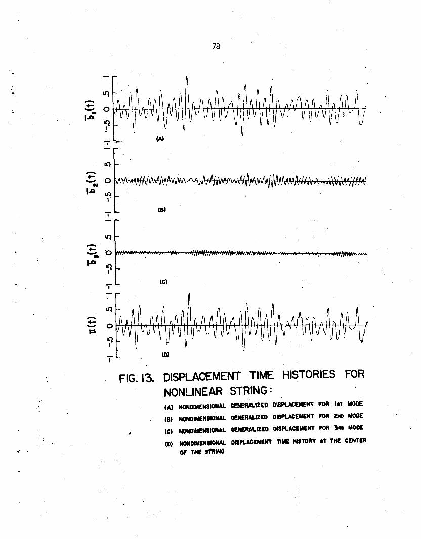
dictor-Corrector method. Fig. 13 shows the simulated samples of the
displacement at the midspan. The first three time series are the
generalized displacement histories for the 1st, 2nd, and 3rd modes
of motion respectively. The fourth one gives the actual displacement
due to all three modes of motion at the center of the string. The
root mean square aQ of nondimensional response
at the midspan is plotted as a function of the root mean square
of nondimensional forcing function
f(x,t) =_
in Fig. 14. The total number of 2000 time points with time increment
of 0.025 sec. were used for response calculation. For the sake of
comparison, the response of the linear string was also plotted on the
Fig. 14.
Conclusion
By comparing the results with the one obtained by Shinozuka [8]
for the same problem, it is found that they are very close. This
demonstrates the usefullness of the FFT simulation method. It is very

77
!«*-"
£j
o
h i *• ? - i f . ';IL y fcifl A«-:^ .ufe j ^1^ B ^^ .'ii ^ >• -W V H^s M i i; - « ii'psj'' • ilM i ^u^!j
U)
•a
a.
m
(C)
lUji iiI'IY"' vyi
WlJiitv J^/lfflJV'M »• V wy / '/ 'An
FIG. 12. GENERALIZED FORCES FOR NONLINEAR
STRINQ:(A) JWNDIMENSJONAL GENERALIZED FORCE FOR 1ST MODE
(B) NONOIMEHStONAL GENERALIZED FORCE FOR 2m> MODE
(C) NONDIMENSIONAL GENERALIZED FORCE FOR 3m MODE
78
in
o Av . - ' l / l / l / 1
(B)
FIG. 13. DISPLACEMENT TIME HISTORIES FOR
NONLINEAR STRING:(A) NONDtMENSIONAL GENERALIZED DISPLACEMENT FOR Irr MODE
(B) NONDIMEN3WNAL QCNERAUZED DISPLACEMENT FOR 2ND MODE
< (C) NONDIMEN8IONAL OENKRALI2ED DISPLACEMENT FOR Sm MODE
(0) NONDIMEN8IONAL DISPLACEMENT TIME HISTORY AT THE CENTER
OF THE STRINO

79
8(O
±0
0-J
z
zI
I I
I
O
0)
*
•—
o
CD•
O(0O
iqdrod
CVJd
OJ
00OCDOCSJ•
o
od
oc>
OXLUUJ
5oi
o_c•M<u
-QCD
03QJ
l/icoO
-(O
)t-0)c-Eo-ocfOs-<o0)t:
o -g
O)
_S
§
DC .J2(Oo
.o
lN3W
30V
1dS
ia
HV
NO
ISN
3lNia-N
ON
dO
SIN
d

80
interesting to note that total computer time for 2048 simulated
points was less than 2 minutes which shows the advantage of time-
saving due to FFT method. To simulate the same number of points
using trigonometric model takes about 30 minutes of computer time.
Example 3. Nonlinear Panel Response Due to Turbulent- Boundary Layer.
The random vibration of a flexible plate immersed in a fluid
flow on one side and backed by a fluid filled cavity on the other
side has been considered in this analysis (Fig. 15). The nonlinear
plate stiffness, induced in the plate by out-of-plane bending and
the mutual interaction between the external and internal fluid flow,
is included. The same problem has been considered by Shinozuka [1]
where he used multidimensional simulation method to find the deflec-
tion at the center of the plate. In the present work, the
FFT simulation approach has been used to do the response analysis at
the center of plate. The results are compared with the ones obtained
in Ref. [1].
The deflection w of a simply supported plate having geometric
nonlinearity is described, in dimensionless form, by two partial
differential equations
V4W = $yy- + *t#fyy -2*jy - W~
- 3 w t - w ^ - + p ' + p e + pc (4-41)f\
V4! = 12(l-v2){w5<y - w yy} (4-42)
with-boundary conditions

81
PLATE
Fig. 15. Problem'geometry for nonlinear plate vibration due toturbulent boundary layer pressure.

82
w(0,y/f) = w(l,y,t) =0
w(x,0,t) = w(xM,D =0
ltt) = 0
yyt) = 0
where x~ = x/a, a = plate length
y = y/b, b = plate width
w = w/h, h = plate thickness
$ = nondimensional airy stress function for membrane stresses
v = Poisson's ratiot 1 /D
t = nondimensional time = -H/— whereabr PD = Eh3/12(l-v2), plate stiffness
E = modulus of elasticity
3 = damping co-efficient
a2b2
p = . p p(x,y,tf) where p(x,y,t:) is turbulent pressure
2h2Pe = ^p pe(x,y,:t) where pe(x~,y,tf) is fluid pressure due to
external flowty f\
pc = ^TQ-p^tx.y.T) where pc(5T,yYt) is fluid pressure due to
cavity flow
In solving Eqs. (4-41) and (4-42), the plate deflection w is expanded
in terms of the normal modes of the corresponding linear plate:
w(x",y,T) = E E bmn(lf)sin nmxsin mry (4-44)m n
where bmn(tf) is the modal amplitude.

83
After the stress function $ is evaluated [19], the assumed modal
solution is satisfied in the Galerkin sense by computing its integral
which is average weighted in turn by each term of Eq. (4-44). The
result is a system of simultaneous nonlinear integral-differential
equations for b—.(t) which involve the following generalized forces
_ .?u2 rl rl•Fmn(t) = TIT" p(x,y,tf)sin mrrxsin nhU J0 J0
a rl rlh ., 9 P VA jy , t j s in nrnrxsi
p II J J
. ! . ! _ _1 1 n fv v T^"in imr¥-in i i |j \ A ,jr » uy b i n iiniAoi
hp°°a- ^o ^o
irydxdy
n mryd^dy-
n mryd^d-
(4-45a)
(4-45b)
(4-45c)
where pbo = free stream density
DO, = mean external flow velocity
ac = velocity of sound, cavity flow
To promote computation ease, a two mode approximation corresponding .
to x coordinate and one mode approximation corresponding to y co-
ordinate to Eq. (4-44) has been assumed. Then the solution for $ [19]
satisfying Eq. (4-42) is given by
+ [(a2 + v)bn2 + (a2 + 4v)b21
2]a2x2}
En2a2 bn2rr~7i cos 2irx - biiboicos irx
bllb21 b212 -STTX + - c o s 4-rrx]
(4'46)

84
where a = jr
Substituting Eq. (4-46) and Eq. (4-44) into Eq. (4-41) we get the
following set of equations
b^ + 3^ + (C1Q + C-,^-,2 + C12b22)b11
+\CFC + AFi6) (4-47a)
= 4(F2 + ACF2C + AF2
e) (4-47b)
where b-j = b-j ^, bg = b2-|, Fj = FJ-J , F2 = F2-j, etc.
C = (a + l)2ir4IU Q
r - ( a. 4\2 4U20 ~ (a + ~J *
cll = |^4[(l-v2)(a2 + 72) + 2(2v + a2 +*r Ct (X
2(5v + a2 +
c21 = c12
+ 2(8v + a2 + 4)]a
3-j and $2 are the damping coefficients for the first and second mode
respectively. The generalized aerodynamic force of the external flow
is given by
Fm6 = * Q™, (4-48)r
where Q^ is given in references [20] and [21]. For high mach

85
numbers, Eq. (2-48) can be approximated to
[Embr(t] + Pmlb r(t)] (4-49)r
where
- 0 for r = m
for r = m
= 0 for r=f m, M = mach no.
Again based on Ref. [21], the generalized cavity force is given by
Thus having obtained the approximate expressions for the generalized
forces due to external flow and cavity flow, we proceed to find the
generalized forces due to turbulent pressure fluctuations as follows
by usingthe FFT simulation technique: the semi-empirical formula of
cross-spectral density for subsonic boundary layer turbulence is
given by [22]
.-6S(w,k-| ,k2) = 0.715 x 10
0.8exp(-0.47w^-)Uoo
(4-51)
for 0 £ w < °°
where, w = freq. in radians, k-j and k2 are wave numbers in the x and y

86
directions respectively. Uc = 0 . 6 5 U», q = dynamic pressure =2
pU» /2, c = boundary layer thickness.
Let £-| = x2 - x-j
Then the spectral density function
rJ
0.1w 0.715w j- -
IT Uoo
where C0 = 3.7exp(-2jg-)+ 0.8exp(-0.47S - 3.4exp(-87;§)Uoo (fo ^Joo
(4.52)
Now, the generalized force due to turbulent pressure fluctuation is
given as
F (t) = «2b2 f1 f1 ,_ -h
r rJ J PtxT^.Dsln'o 'o
sin m2Try,dx-j ,dy -j (4-53a)
f1 f1P(x2,y2,t + T)sin
J n J n
sin (4-53b)

87
Then
n * n « n * n
x sin m-jTTXiSin moTryiSin
or,
x sin m-|Trx, sin
(4-54)
where R,,, m n n (T) is the cross correlation function of the generalized
force and Rp()T-j ,x~2,y^ »y2»T) is the cross correlation function of the
turbulent pressure fluctuations.
Taking the Fourier Transform of both sides of Eq. (4-54) we get
x sn m-j-n-
(4-55)
where Sm m n n (w) and S(w",Ci.Co) are the spectral density functionsllinllloMi >*O • ^
of the generalized forces and turbulent pressure fluctuations
respectively and w is the nondimensional frequency.
Nondimensionalizing Eq. (4-52) with respect to w, £-j and
stituting in Eq. (4-55) for S(w,Ti »O we get

1 1 i i — n Iwa .— — ,0.715wbx r1 f1 f1 [Vlxz-x!.|^e-|y2-yi|—or-
•'o •'o •'o •'o
., ,awx s ' -sin rn-iTTX^sin m2"F]Sin njirx^
x sin n2Try2d)ridX2dy^d72 (4-56)
In order to solve the integral in Eq. (4-56) we proceed as follows:
let
IVl = Jo
sin m-iTTX-jsin n-|irX2dxidx2 (4-57a)
rl ,_ _ .0.715waI 6 - | y 2 - y i D C
'osin n^TTyiSin n2Try2dyi dy2 (4-57b)
then
,1
2 -c- •'o
ri= J
-0_.lwa
0.1 wa- i -°.-.'lw.?x- iw§=7e -DT*! 1
e ^^2e-JD?<2
xl
x sin n-|TrX2dX2]dXi (4-58)
Evaluating the integrals inside the square bracket separately:

89
— O.lwa- ." -
e e sin n-iTrx2dx2
•r' nO.lwa-
e c cos l osin
O.lwa-2
e sin. fAl uc
•f
0.1wa-
e cos
0.1wa-.pi ~°c~^2iJ e
Jo
O.lwa_
- cos
cos (n^ + g3-)^
wa
T2
wa
A
O.lwa
"~B
1 waf (^TT - Uc)
B
COS

90
Q.lwa 1,Uc B
O'.lwa-
A
+ (lyr* )s1n (njir + j
0.1 wa J-i'~OT~A}
where, A = (Q-lwa.)? + (n + wa}2^*C ' ^C
Integral Table [23] was used to evaluate the above integrals
Now, we want to evaluate
-0.1 wa_ wa—~ ~r
_ e e sinxl
-O.lwa-?
wa- _.• i; •" cos
-0.1 wa-Uc
X2" -|-e "{cos (n--rr - " cos ("^ + -
C . D
-e
-O.lwa . , wa»— / wax / wav--y—sin (n-j-rr - u^Jx-j - (n-jir - ^-)cos (n-jTr - u^;x1
B

91
-O.lw—
-0.1wa wa»— wa.-
i -.
A
where,
-O.lwa
C = e uc {
-O.lwa
D - e U c ' <
-O.lwa
(n,, - f ) - (n^ - g|)cos (»,, -
E = e c
uc « "t
-O.lwaF = e
Uc {'V^cos (niir + ^v*
Multiplying Eq. (4-59a) by
adding them, we get
-Q.lwa- 0-1wa- wa-
[e-uT^lfXleUc V^2s1n
and Eq. (4-59b) by
O.lwasin
(4-59b)
and

92
.lwa .,
-O.lwa- O.lwa-
-0.1wa-
De
,1r0.1wa.
.1 rQ.1waUc °s
-O.lwa- 0.1 war,1 ,-O.lwa ~TF~~X1 . ./"OrFe
-O.lwa- O.lwc^.f0.1waQ ~0c xl pp Uc 1-,
'2Bl~Dc~^
Substituting Eq. (4-59c) in Eq. (4-58) and carrying out the inte-
gration, we get
T jO-lwa O.lwa,.;2BUC
J6m1n1
(4-59c)
wa wa -O.lwa
0.1 warC . D , Uc ,C2 , D2-,{4A + 4B}e {AT + BT}
-0.1 waO.lwaJ 1 , ~DE~TE1 . Fl,
- 4A}e {AT + BT>O.lwa
Uc •C ^4A " 4BnAT
O.lwa r

93
O.lwa
where
Al =
Cl
Dl
El
FT
Gl
C2
D2
2BUc(nvfTr + ^ir]
«% __ j. Wet M _ wa -
4A 4B J Bi
O.lwa
J % + W}e U° {£T + BT}
-O.lwa• O.lwa/1 1 Io Ur rCl . DliJ "TJ^W ' 4A} {AT + BT}
O.lwa. rF E i Mr fC2 + D2^J 14A " 4B"/e C 1AT FT
wa_,2Uc'
- ) - (11,11 - w)cos (m,ir -
gi)sin
- (ny
(4-60)
. gi) . („,,„ . «|)COS („,,„ +
G2 = - gf) + (V - j"),

94
Now,
,- - ,0.715wb•ju:I_ _ = e - ' -<• sinm2n2 J0 J0
Carrying out the integration we get
Q.715WD
uc
Uc
-0.715wb
+ (-I)"2*1)}] (4-61)
Then
'(I * -' (4-62)
where Im n and Im n are given by Eq. (4-60) and Eq. (4-61) respec-
ti vel y .
Thus, the spectral density function of the generalized force due to
turbulent pressure having been obtained, the generalized forces were
simulated by using the FFT simulation technique.
As pointed out earlier, to work out a numerical example a two
mode approximation in the x direction and one mode approximation in
the y direction was taken. In order to compare the results with ones
given in ref. [l],the following numerical values taken in [1] were used:
a = 10 in., b = 20 in.
d = 5 in. , v = 0.3
p = O.lh lb/in2, E = 107 psi

95
Uc = 0.65 UU, ap = 0.0056 q
pbo = pc = 0.00089 slugs/ft3
aoo = ac = 995 ft/sec
U» = 800 ft/sec,'5 = 0.157 in.
The thickness of the plate was varied in a way to adjust the non-
dimensional pressure, p", for the convenience of illustration. The
damping coefficients 3] and 32 were taken as 1 percent of the
critical damping of the 1st and 2nd modes of linear plate, respec-
tively.
In order to solve the equations (4-47a) and (4-47b), 4096
discrete values of both F](tf) and F ftf) were simulated from the
derived expression for spectral density function using the FFT simu-
lation technique. Eqs. (4-47a) and (4-47b) were reduced into four
first order differential equations, and a modified predictor corrector
method was used to solve for b-| (t) and 2 ) with zero initial con-
ditions. Fig. 16 shows the displacement time history at the center
of the plate and the generalized forces for the first and second mode.
The nondimensional R.M.S. response at the center of the plate versus
the nondimensional R.M.S. pressure is plotted in Fig. 17 with and
without the cavity effect. For the purpose of comparison, response
corresponding to linear plate is also plotted in Fig. 17.
Conclusion
It is seen that the results obtained here compare very closely
with the one given in Ref. [1] for the sub-sonic case. Results obtained
in [1] are based on the multidimensional simulation analysis where

96
oo£
52
Si
8M
H
£LUOLJ-
_U-
§ S
S

97
oOX
oI§sIE<UJ
10oxOroOx00
10gxCD
roOxrogXCM
s_01<o
UJ
trIDCOCOUJ
trQ.
COzUl
o.QotoO)
a> •
«/> "O
c o
o -c
Q +
->in
OJ
OJ LJ_
03CLJD
4-
EO
O
OCOon
T3
(O3
3
in o3
O) r—
«0
S-
J-
3<o
inQ
. «/)E
0)
o s-
cj
n.
10in
•
oqd
lN3IM
30V
ndS
ia 1V
NO
ISN
3WIQ
-NO
N
JO S
Wd

98
Shinozuka has taken only 100 frequency points which looks like a very
small number considering the fact that turbulent pressure fluction
takes place over a wide frequency range. From this point of view,
our analysis seems more accurate because we have divided the
spectrum into 4096 points. The total computer time to simulate 4096
values of both F-j (t) and F2(t) and to obtain 4096 points for both
b-|(tf) and b£(t) was only 3 minutes 30 seconds. It is needless to
point out that the time required to simulate 4096 points for the
generalized forces by using the trigonometric model of simulation
will be much much more. This once again brings out the immense use-
fulness of FFT simulation approach wherever it is applicable.

CHAPTER V
CONCLUSIONS AND FUTURE EXTENSIONS
Two methods of simulation of a multivariate and multicorrelated
random process have been presented and these methods have been
applied to analyze some example problems of linear and nonlinear
random vibration.
Comparing the two methods of simulation, we conclude that both
the methods work very well. The only drawback is the amount of
computer storage, which can become prohibitive if there are too many
correlated processes to be simulated or if a very large number of
discretized points are necessary for analysis. It is noted that FFT
method works much faster in terms of computer time compared to the
.trigonometric model. This speed ratio is directly proportional to
the number of series and discretized points to be simulated. For
example, the time required to simulate the six components of wind
turbulence, with each pf the time series having 2048 discretized
points, was twenty times less in the case of FFT method compared to
the trigonometric approach. But FFT approach has a drawback in that
the number of time points is equal to the number of frequency points
and we cannot restart the simulation at any given time t. It has to
start at t = 0. Also, the time interval is related to the frequency
interval. The trigonometric approach does not suffer from these
99

100
disadvantages. Here, we can start the simulation beyond any given
time and also the time interval is not dependent on the frequency
discretization. Thus, we see that whereas the FFT method has a
tremendous advantage in terms of computer time, the trigonometric
method can be more useful in certain cases.
As to the usefulness and importance of the simulation technique,
we conclude that it offers probably the best means of performing the
nonlinear response analysis of random vibration problems when the
spectral function for the forcing function is specified. In light
of the review study in Chapter II, we feel that the simulation approach
and particularly the FFT method gives a much faster solution with
lesser number of constraints. It is noted that FFT method works as
well as the ones in Ref. [1, 6, 8] for analyzing the nonlinear re-
sponse and this approach is much faster than that of Shinozuka
[1,6,8].
The methods of simulation presented here can be extended to in-
clude multidimensional homogeneous and nonhomogenous processes. For
example, writing
m N-| N2 Nn
p=l k^l k2=l kn=l
X COS [W-i. t + Wo,, XT + +
x sin [W|. t + w2. x-| + ... + wn. xn + (k-j ,k2...kn)]
[5-1]

101
one can simulate a multivariate multidimensional process using trigo-
nometric method. Shinuzuka [6, 8] has already extended his trigono-
metric model to include the multidimensionality and the above proposed
extension will not be much of a problem. But it will be really
exciting to extend the FFT approach to a multivariate-rnulticiimensional
case. It does not seem very difficult particularly when the sub-
routine HARM can take care of up to 3-dimensional inverse Fourier
Transform. We feel that it should work without trouble, but it does
need a little closer look. It might be also interesting to extend the
FFT approach to include the nonhomogeneous process by utilizing the
concept of evolutionary power spectrum. This will be useful in simu-
lating trasient and siesmic response and will also lead to considerable
time saving over Shinozuka's method [8].
There are lots of other areas in which the simulation approach
can be very useful and about which we have not discussed in this
dissertation. For example, in the area of reliability analysis and
in the response analysis of structures when the spatial variation of
material properties are specified. These are some of the many areas,
the simulation technique and particularly the FFT approach can be
extended. These extensions look very practical.

REFERENCES
[1] Vaicatis, R., Jan, C. M. and Shinozuka, M., "Nonlinear PanelResponse from a Turbulent Boundary Layer," AIM Journal,Vol. 10, No. 7, July, 1972.
[£l Goto, H., Doki, K., and Akiyoshi, T., "Artificial EarthquakeWaves by Computer," Proceeding of Japan EarthquakeEngineering Symposium, 1966.
[3] Amin, M. and Ang, A. H. S., "Nonstationary Stochastic Model ofEarthquake Motions," Journal of Engineering MechanicsDivision, ASCE. Vol. 94.
[41 Liu, S. C., "Dynamics of Correlated Random Pulse Trains,"Journal of Engineering Mechanics Div., ASCE, Vol. 96,Aug., 1970.
[5] Hoshiya, M. and Tieleman.H. W., "Two Stochastic Models forSimulation of Correlated Random Processes," V.P.I. Tech.Report, VPI=E-71-9, June, 1971.
[6] Shinozuka, M. and Jan, C. M., "Simulation of MultidimensionalRandom Processes II," Tech. Report No. 12, ColumbiaUniv., N.Y., April, 1971.
[7] Borgman, L. E., "Ocean Wave Simulation for Engineering Design,"Journal of Waterways and Harbors Div., ASCE, Vol. No.WW4, November, 1969.
[8] Shinozuka, M., "Simulation of Multivariate and MultidimensionalRandom Processes," Journal of Acoustical Society ofAmerica, Vol. 49, No. 1, January, 1971.
[9] Ariarathan, S. T., "Random Vibration of Nonlinear Suspensions,"Journal of Mechanical Enqr. Science, Vol. 2, pp. 195-201(1960).
[10] Caughey, T. K., "Derivation and Application of the Fokker-Planck Equation to Discrete Nonlinear Systems Subjectedto White Random Excitation," Journal of AcousticalSociety of America. Vol. 35, No. 11, 1963.
102

103
[11] Caughey, T. K., "Equivalent Linearization Technique," Journalof Acoustical Society of America, pp. 1706-1711 (1963)
[121 Crandall, S. H., "Perturbation Technique for Random Vibrationof Nonlinear Systems," Journal of Acoustical Society ofAmerica, Vol. 35, No. 11, Nov., 1963.
[13] Tung, C. C., "The Effects of Runway Roughness on the DynamicResponse of Airplanes," Journal of Sound and Vibration,Vol. 5, pp. 164-172 (1967T
[14] Foss, K. A., "Coordinates Which Uncouple the Equations ofMotion of Damped Linear Systems," Journal of AppliedMechanics, Vol. 25, pp. 361-364 (19587!
[15] Yang, I., "Stationary Random Response of Multidegree-of-FreedomSystems," Ph.D. Thesis, California Institute ofTechnology, submitted March 10, 1970.
[16] Blackadar,A. K., Dutton, J. A., Panofsky, H. A. and Chaplin, A.,"Investigation of Turbulent Wind Field Below 150 MAltitude at the Eastern Test Range," NASA CR-1410, August,1969.
[17] Panofsky, H. A., "Properties of Wind and Temperature at RoundHill, South Dartmouth, Massachusetts," Research andDevelopment Tech. Report ECOM-0035-F, Penn. State Univ.,Univ. Park, Penn., Aug., 1967.
[18] Fichtl, G. H. and Mcvehil, G. E., "Longitudinal and LateralSpectra of Turbulence in the Atmospheric Boundary Layer,"AGARD Conference Proceedings No. 48, NATO, Munich, Sept.,1969.
[19] Bolotin, V. V., Nonconservative Problems of the Theory ofElastic Stability, Pergamon Press, 1963, pp. 280-289.
[20] Dowell, E. H., "Generalized Aerodynamic Forces on a FlexiblePlate Undergoing Transient Motion," Q. Appl. Math., Vol.24, 1967.
[21] Dowell, E. H., "Transmission of Noise from Turbulent BoundaryLayer Through a Flexible Plate into a Closed Cavity,"Journal of Acoustical Society of America, Vol. 46, No.1, 1969.
[22] Bull, M. K., "Wall-Pressure Fluctuation Associated with Sub-sonic Turbulent Boundary Layer Flow," J. Fluid Mech.,Vol. 28, Part 4, 1967.

104
[23] Gradshteyn, I. S. and Ryzhik, I. M., Table of Integrals Seriesand Products, Academic Press, 1965.
[24] Bendat, J. S. and Piersol, A. G., Random Data: Analysis andMeasurement Procedures, Wiley-Interscience, New York,1971.
[25] Lin, Y. K., Probabilistic Theory of Structural Dynamics,McGraw-Hill Book Company, New York, 1967.
[26] Meirovitch, L., Analytical Methods in Vibration, The MacmillanCompany, London, 1967.
[27] Dutton, J. A., Panofsky, H. A., Deaven, D. C., Kerman, B. R.and Mirabella, V., "Statistical Properties of Turbulenceat the Kennedy Space Center for Aerospace Vehicle Design,"NASA CR-1889, August 1971.
[28] McVehil, G. E. and Camnitz, H. G., "Ground Wind Characteristicsat Kennedy Space Center," NASA CR-1418, Sept. 1969.
[29] Maestrello, L., "Measurement and Analysis of the ResponseField of Turbulent Boundary Layer Excited Panels," J. ofSound and Vibration. 2, 1965, pp. 270-292.
[30] Shinozuka, M. and Wen, Y. K., "Monte Carlo Solution of Non-linear Vibrations," AIAA Paper No. 71-213, AIAA 9thAerospace Science Meeting, New York, 1971.
[31] Fung, Y. C. and Barton, M. V., "Shock Response of a NonlinearSystem," J. of Applied Mech., Sept., 1962.
[321 Gardener, N. J., "Response of Cooling Tower to Turbulent Wind,"J. of Strc. Div. of ASCE. Oct., 1969.
[33] Vickery, B. J., "Wind Action on Simple Yielding Structures,"J. of Engr. Mech. Div. of ASCE, April 1970.
[34] Beer, F. P., "On the Response of Linear System to Time-Dependent,Multidimensional Loadings," Journal of Applied Mechanics,March 1961.
[35] Shinozuka, M. and Astill, C. J., "Random Eigenvalue Problemsin Structural Analysis," AIAA Journal. Vol. 10, No. 4,1972.
[36] Hasselman, T. K. and Hart, G. C., "Modal Analysis of RandomStructural Systems," J. of Engr. Mech. Div., ASCE, June1972.

105
[37] Proceedings of Seminar on Wind Loads and Structures, sponsoredby NSF, Japan Soc. for Promotion of Science and Univ. ofHawaii, Oct., 1970.

APPENDIX A
1. Random Variable and Probability Distribution Function
Let X be any random variable which varies with statistical regu-
larity. Since X is a random variable, any function of X is also a
random variable.
The first-order probability distribution function of X can be
described by a graph as in Fig. A-l which shows the probability den-
sity function p(X). The hatched area gives the probability that X
lies between a and b. ItMs apparent that the probability is zero
that X actually assumes any given value x. Also we havei
p(X)dX =1- (A-l)i . . .
The cumulative distribution function (CDF) defines the probability of
occurrence of a value of X less than or equal to a given value x, i.e.,
P(x) = j p(X)dx. (A-2)-00
According to fundamental theorem of integral calculus,
• P(x) (A-3)
wherever this derivative exists.
Properties of CDF
(1) CDF is a non-decreasing function of x
(2) P(x) varies between 0 and 1 as x varies from -» to °°. Thus
P(-») = 0 and PH = 1.
Several random variables X,, Xp, . . .X are said to be jointly dis-
tributed if they are defined as functions on the same sample description
106

107
POO
0 X
Fig. 1-A. PDF of Continuous Random Variable X.

108
space. We shall refer to p(X,, X 2 , . . .X ) as the joint probability
density of these random variables. Thus, the probability that a, <
X, < b,, a0 < X0 < bo s . ..a., < X^ < b_ is given by1 12 2 2 n n n 3 J
f1 [ 2...[ n p(X1 ,X2 , . . .Xn)dX1dX2 . . .dXn . (A-4)J a_ J a _ J ;>ll '"2 ~an
Also,
j ] • • • ] p(X1,X2,...Xn)dX1dX2...dXn = 1 . (A-5)—oo — oo »oo
The joint probability distribution of two random variables X, and X2
is given by
p(XrX2) (A-6)
and
p(a-, < X, < b, and a2 < X2 < b,,) •
= I ] I 2 p(X1,X2)dX1dX2 (A-7)
Supposing that X is now a random function of spacial coordinates
x^ or time t, the first and joint probability distribution functions
defined above are valid for any given values of x_ or t. That is, the
probability that X (x or t) lies between a and b is given byrb
p(X(x, or t))dX(x or t) (A-8)^a
and
P(x) = J p(X(x or t))dX(x or t) • (A-9)
—CO
2. Mean. Mean Square, Variance and Standard Deviation
The ensemble average

109
= Jyx = E[X] = / X p(X)dX (A-10)
—CO
defines the mean of X or the expected value of X. The operator E is
used to denote this kind of average. The mean square value of X is
given by
E [X2] = I X2 p(X)dX- (A-ll)
An important statistical parameter is the variance of X which is the
ensemble average of the square of the deviation from the mean. Thus
the variance of X is given by
a2 = E [(X-yx)2] = f(X-yx)
2 p(X)dX
An alternate expression is
a2 = E[X2] - yx2 • (A-13)
When the mean is zero, the variance is identical with mean square.
The square root of Eq. ( 13 ), that is a, is called the standard
deviation. The co-efficient of variation is defined by
V- 'g - (A-14)yx
which tells the degree of variation.
3. Random Process
Let us consider random functions X(t) and Y( t ) in which t
represents any variable, say, special co-ordinates or time.
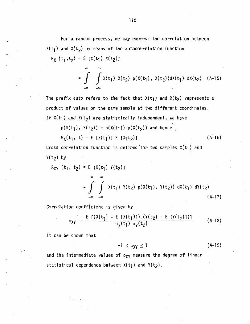
no
For a random process, we may express the correlation between
X(t-j) and X(t2) by means of the autocorrelation function
Rx (trt2) = E [X(t}) X(t2)]
oo • oo
= J f X(t!) X(t2) pttUT), X(t2))dX(t1) dX(t2) (A-15)
-00 -CO
The prefix auto refers to the fact that X(t-|) and X(t2) represents a
product of values on the same sample at two different coordinates.
If X(t^) and X(t2) are statistically independent, we have
p(X(t1), X(t2)) = p(X(t!)) p(X(t2)) and hence
RxU^ t) = E [X( t ! ) ] E [Xit2)] (A-16)
Cross correlation function is defined for two samples X( t - [ ) and
Y(t2) by
t2) = E [X( tT ) Y(t2)]
OO OO
= f f x(tl) Y(t2) P(X(t i) , Y(t2 ) ) dX(t ! ) .dY(t2 )
—OO —CO (A-17)
Correlation coefficient is given by
E [(X(t,) - E [X(t1)])_(Y(t2) - E [Y(t2)])]PYY = ! /. v /.i— (A-18)MXY ax(t-|) ay(t2)
It can be shown that
-1 < PXY £ 1 (A-19)
and the intermediate values of PXY measure the degree of linear
statistical dependence between X(t]) and

in
4. Stationary Random Process
A random process is said to be stationary if its probability
distributions are invariant under a shift of the co-ordinates. In
other words, the family of probability densities applicable at t-j also
applies at ^- In particular, the first order probability density
function p(X) becomes universal distribution independent of time.2
This implies that all the averages baseed on p(X) , say, E [X ] and 0 ,
are constants independent of time.
For a stationary process, the autocorrelation or cross cor-
relation functions become functions of the difference between t, and
t2 and independent of t, or t2.
Therefore, for a stationary process, Equation (A-15) becomes
RX(T) = E [X(t!) X(t!+T)]s T = t| - t2 (A-20)
and Equation (A-17) is
RXY(T) = E [X(t-,) Y(t! + T ) ] , T = t} - t2- (A-21)

APPENDIX B
Fast Fourier Transform
^ Restricting the limits to a finite time interval for the record
x(t), say in the range (o, T), the finite range Fourier Transform is
defined as
T
X(f, T) = J x(t)e'J'2Trftdt (B-l)
oAssume now that time x(t) is sampled at N equally spaced points a
distance h apart, then for arbitrary f, the discrete version of
Equation (B-l) becomes
N-lX(f , T) = h I xn Exp[-j 2ir fnh] (B-2)
n=0
Selecting the discrete frequency values as
fk = kf = T= Nh k = 0, 1, 2, ... N-l (B-3)
At these frequencies, the transformed values give the Fourier com-
ponents defined by
Y _ X(fk, T) N-- j xn exP I"
k = 0, 1, 2 ..., N-l (B-4)
where h has been included with X(f|<, T) to have a scale factor of
unity before the summation. Note that results are unique only out to
112

113
k = 2 since the Nyquist cutoff frequency occurs at this point. Fast
Fourier transform (FFT) methods are designed to compute these
quantities, X^, and can also be used to compute the co-efficients of
the regular Fourierseries Aq and Bq in the expression
N/2xn = x(nh) = Ao + 2 Aq cos(^-pL)
q=l
N T2 ~
+ S Df, f 4 M / tTTQn \ / n r \•* bq sirU .." ) • (B-5)q=l N
To simplify the notation further, let
w(u) = exp [-j p] . (B-6)
Observe that w(N) = 1 and for all u and v,
w(u + v) = w(u) w(v) • (B-7)
Also, let
X(k) = Xk and x(n) = xn (B-8)
Then Equation (B-4) becomesN-l
X(k) = £ x(n) w(kn), k = 0, 1, 2, ... N-l « (B-9)n=0
Equations (B-4) and (B-9) should be studied so as to be easily
recognized as the Fourier transform of x(n) when x(n) is expressed by
a series of N terms. Such equations require a total of approximately" O
fr complex multiply-add operations to compute all of the X(k) terms
involved.
Fast Fourier Transform procedures are now based upon decomposing
N into its composite (nonunity) factors, and carrying out Fourier
transform over the smaller number of terms in each of the composite

114
factors. In particular, if N is the product of p factors such that
N = irr.,- = r^2 ... rp (B-10)
i = 1
where the r's are all integers greater than unity, then it can be
proved [24] that X(k) in Equation (B-9) can be found by computing
in an iterative fashion the sum of p terms,
N 9— Fourier transform requiring 4r-j real operations each,
N 9— Fourier transform requiring 4r? real operations each,r2j (B-ll)
N 9— Fourier transform requiring 4rD real operations each.rP H
Hence the total number of real operations becomes
P4(N + Nr2 + Nr3 + + Nrp) = 4 Z r2 (B-12)
The resulting speed ratio of these FFT procedures to the standard
method is then2
speed ratio = — p = -^— (B-13)4N Z ri 4 E ^
speed ratio for powers of two:
If N = 2P, then z r,- = 2p = 2 logo Ni=l
In this case, the speed ratio by equation (B-13) appears to be
N Nspeed ratio =

115
However, a doubling of the speed can be achieved in practice by
noting that the values for w(kn), when N is a power of 2, all turn
out to be +1 or -1, so as to yield a higher speed ratio of the order
of
speed ratio = Jj- (B-14)
For example, if N = 2'^ = 8192, Equation (B-14) gives a speed ratio
of i^ 158.

APPENDIX C
Expanding Eq. (3-14), with H(W|<) being a lower triangular matrix, one
obtains
+ Hm"n + •••- Hmn"nn« for n < ra,
Gmm=
From Eqs. (3-22a), (3-22b), and (3-3) and (C-l) one can see that
m th component process is simulated from Hmp(w|<) (p = 1, . . . , m) and
the coherence between the m th component and n th component with
n < m is generated by (w ) and Hnp(w|<) (p = 1, 2 ..... n). When
a vanishing minor is due to a zero mean square density of, say, the
m th component process at a frequency w^, then the elements of cross-
spectral density associated with this component are also zero at this
particular frequency. It is easy to show that a sufficient condition
for this case is
Hmn(w|<) = 0, for n = 1, 2, ... m
Hnm(w|<) = 0, for n = m + 1, .... M
The remaining elements of Hmn(w|<) are then determined from the sub-
matrix obtained by deleting the m th row and m th column from the
matrix G(wk).
A coherence of unity between two component processes (the m th
and the (m + 1) th) at a frequency w^ will also give rise to vanishing
116

117
principal minors: This implies a complete linear dependence at this
frequency between the two processes and hence the existence of the
transfer function 3(wk) such that
G^, m+l(wk) = |3(w)|2Gmm(wk)
(C-2)GJJ, , m+1 (v,'k) = 3 (w} Gflim (wk)
Therefore, at this wk, it can be shown that G(wk) will take the
following form:
Gin G-i j G-i ,j+l G,..ii ij i ip/i
Gill GMj G>> 1+1 GMMMl Mj M, MM
G-i T G-i . 3G_- _• G-i MII Ij ij in •
G^i G.:,- 3G-;-; Gn*M_ _ .o _ (C-3)
1
GM1 GM.i 3GM.i GMM
In this case, H(wk) can be solved for a particular frequency in the
following fashion.
First, reduce the size of both matrices G(wk) and H(wk) by
deleting the (j + 1) th row and (j + 1) the column, then solve for
the reduced H(w. ) from the reduced GCw^), by the method mentioned in

118
Chapter I I I . Final ly , the deleted elements of H ( w k ) , as can be seen
by direct substitution in Eq. (C-l ) , are given by
Hj+ 1 ,p = FH.jp) for p = 1, 2, ... j
H j+1 ,j+l = 0 , (C-4)
H,,,j+l = 0, for p = j+2, M
If two component processes, again, say, the j th and (j + 1) th,
are completely correlated, then $(w) as defined for the previous case
will reduce to a real constant $0 independent of the frequency. This
will lead to Dpfw^) = 0, p = j + 1, ... M, for all frequencies. For
this case, it is necessary to simulate only m - 1 component processes
with the (j + 1) th removed from the system, since it can be obtained
by
fj+1(t) = 00fj(t)
With the proper combination of the above procedures, it is possible
to deal with the following situations:
(i) more than one component of GCw^) vanishes;
(ii) more than two components are completely coherent or
correlated;
(iii) the combination thereof.

APPENDIX D
COMPUTER PROGRAM
This section of the report deals with the listing of some of
the important input parameters in the computer programs included.
On the left-hand column is the computer language (FORTRAN) symbol and
on the right-hand side, just opposite, is the equivalent variable
used in the derivation of the equations in Chapter III and Chapter
IV.
Listing for Program for Simulation by Trigonometric Method:
K KA, frequency index
ornp(k) ALPHA(I,KK,KA), deterministic phase angles
Wu WU, upper cut-off frequency
M£ WL, lower cut-off frequency
Gmn S(I,J), element of spectral density function
Hjn- HHH(I,J), elements of lower triangular matrix
amp» kmp AA(I,KK,KA), BB(I,KK,KA), random Gaussian variables
Aw DW, discretized frequency interval
m KK,- number of time series
£p, TV VI , V2, random number generated by Gauss subroutine
At DT, time interval
fm(t) F(I,JJJ), representation of time series
119

120
Listing for Program for Simulation by FFT Method:
K KA, frequency index
G(I,J) S(I,J), input spectral density function
Hp k HHH(I.J), elements of lower triangular matrix
np|<, L^ Z1(K), Z2(K), independent Gaussian random numbers
Cp XI(K), complex random number
h DT, time interval
Xpk DDX(I,KA), elements of complex random vector
fpn F(I,J), time series representation
Listing for Program for Nonlinear Response
Analysis of String
Of SIGF, standard deviation of the forcing function
L TL, length of the string
a ALPHA, a constant
T0 TO, initial tension in the string
p ROE, density per unit length
w-] , w2, w3 Wl, W2, W3, natural frequency of vibration for
1st, 2nd and 3rd modes respectively
A AR, area of cross section
S0(w) SO(KA), spectral density function of actual force
Smn(w) S(I,J), spectral density of the generalized force
fm(t) F(I,J), generalized force representation
bn(t) AN(t), derivative of modal displacement
bn(t) BN(t), modal displacement

121
bn(t) ANPR(t), second derivative of the modal dis-
placement
Listing for Program for Nonlinear Panel
Response Problem:
3-i BET1, percentage of critical damping for 1st mode
of vibration
32 BET2, percentage of critical damping for 2nd mode
of vibration
cfp SIGP, r.m.s. pressure of boundary layer pressure
fluctuations
Uoo UINF, mean external flow velocity
a SA, plate length
b SB, plate width
v GNU, Poisson's ratio
Uc DC, convectional speed
M CM, mack number
p ROE, plate density per unit area
d SI, cavi ty depth
u SV, sound velocity
C ' XSI, boundary layer thickness
F ALP
D RIG, plate stiffness
Ac DEMC, constant
X DEM, constant

122
q SQ, dynamic pressure
C0 CONST, constant

123
'X^LU^JT"
' — (
OI— *
'-Xi —retou.,oo•
1U:
(J
CtXa.5.
OC;
2<i
aRP-<tT t1.1;
C£
acQu-*'_j^35;
u_O2;O*• «
h—<^_J
^>rV
w4
Vi
^ "
O
*Z
«•
o
«~
-»
•• »• -4-
•03 —
O
» v
C C
\i —
.vo ~
>~- oc,—
x -H
>r<
••
U, O
O-
•<)
^^ *k^
— J
*— '
--Ti ^
'<r >• <t~ u.».
c ••
—
f\j ~•O
^ • oo
«• •> -o
-o -* ~
o—
vO
U
- (V
c? »
^ ^^•• \o «~ m
— • •—
\o u_vO
X
~"
•>
«• x-x —
•-c x x o
•—
••
•• u~
cj — » »~
OxC
O
<NJ
•— —
Ii.- I
JS -
— X
- —
c; —
k coIT
1. ^ O
-t
OC
- ~
O
O
Q<N
-O
vO
f\l »
—
^
^ x
>
isJ vO \u
^J" >-
•">K
•<
-••. a
>
co
-. "
X
• rO
"•C ^
cO ^0
^
r^ 00
•• ~
03
>f
X
1
»V
J•i;
<;
•" O
•>
2"
•~
^ —
INJ x
x ^oa
-.Q o
— • x
~- -s.*"*
v.
. !">
fO
«.
(\
Xk^ ~g
<jo -o u.
c> r-
— o
2T •«
»
» ^O
U
>N
- _
J-^
CT sO
*•"•* fO
jS
^"
i— ~
»
or. x ^r c
i of
Q
CO
sO O
"^
UJ
»— 4 c-
^3
OO
2T
».
«-
O_
JO
»»
2o
O»
<X
ajs
O<
fMO
.orO
Q^
«—
||
•-. — »
^t- 5: —
< —
s .0
ii ii
ii ii 3: ii
ii ii
Uj>
-->
-rM
O(IZ
5_
)Z
3:Q
V-<
s.!:
s: O
»•
a. u
-z
^;j:x
CiQ
O3
.cx
^|^j
r-TLLX1——
J •—
•JS
00
• 3
LU
O O
QII
•"•
<t 0
<
S<C •
OC
. <l
*• »™
* k—
»ksC
>—
^
| ^_;
^-(
•
» 1
C S
i Li.'
II—
' •-!
•• X
Q-
1-1
II u «
-y>
3«i <C
*" H
- O
f*- !*• X
<T
O -^
Q. v: a
O O
_J ~
- Z. O
•ft C
C
J O
O
is)
• «
• -sQ
->-.~
5O
O
oc
inc
cm
o^
H ii
cc cr *j- -~t o
ex',«^ «^- 4- PW
ro v.
»ir\
•-)
->
• •
• ;sl c
.i «
O••
•• O
'O O
«-
II •-'
O>-< >
-i ,-ri ||
|| {)
^3
|| ,-i
— —
II
-D
OO
SIo
o
|i

124
CJ
0
in•it—Li.
-ftCT.invf"1d
•m•5tO•
Cvl
#»
O-o-—CM-*<t
3~LH~<
fT
,
rv.' -|»
\O#
• •
z; — <
oo
—
i o
* #
•
•— •
— *
-••• to
''JO
c\j z> -~ * •-«
<t sr
•••• o
•"• •*«,:*
U
. Z>
^
O M
u*> -*• I> X
• to
zi c? «•
cc m—
• o
n
--r ^
o«•
O
e —
t\|
«x
»Z
> <N
J r<
^
•— l
• rsjj
oc
-H —
» in
— n
II —
• »s -4 "••
H
O|l
— II
ID T
X
O
O
INI C
D U
-
§~LL(7-in,
7«^•irOf
r\j•H.Q
\•oU
"i
—M•M-
' <rs•Itin^
XJ
•+«
•!?• •
Z) i™
~*u *-
•if «•
*^ ^
M
(N) Z/
"•IS-
X
—
O* U
- Z
) i/-. •»• >
x
C
• O
I)
CO
C
O*
1—
1
« ••» »^ v
O
• u o
m •*• •
•O
C
C >
^ ^-* •* O
00
ITS l(
•«- X» >
t fA
l|
II II
~»
II Z>
**J X O
O
isi O
•«•w«IJ_4fITinjoro•ir0•r\j&
0
O•O—M*23:
oo -tt
enin
in
:n
in o
-H
m
oCO •«
• rsi +
n
«•
« -it
-tr »
•
«•
O «-•
Z>
fH
C —
|O
O—
1
0~
»
•* #
—
«^
oo
<
-»<-»
-it co
<r i—
l (\l
Z)
••»
*f i—
<—
«>
s
•ifX
'^O
—
""vO
f^J
*U
.Z>
1>x
O^
t ^*
CO
^t- >
X
•
•»••O
sJOG
-K-
30
* C
O-K
-_,
_1 _
4
^.
» Q
||
>}•_
<,_
(IT
tV
o
• 1k O
»
*~(M
1«s
. •
• M
C5
OZ
)f\)fO
C\4
"M
O
•O
—IIQ
CQ
<-
I—
• »• in
—
• ||
OU
II
Z>
•-«
II —
>v <M
-
II Z3
'-n0
3
s: n
n
— n
z> s: n
J>
2)IA
.M
XO
O
rNiO
OL
U's
l
IT-
»•it^^
u.•K-
oJ^vlo
ooVr
'.?•'\t
*cr•oin~-rv
l
*5^^f
in^INI +to
•
Z5
•—
IO
—•it
-it"
«««
rs; Z3 —
•!<•?
•"••)<•
u. Z>
t^ -it >Z
, C
- to
~
• o•i;-
-H
tZ
J O «
*>CC
—^
•—II
~- >
xII
.X 0
•K-
,— 1
rri
- — '
•X'
_^v.
r-J
^it'.JE—•itC
>lOr—
1
4-Ot
^^
^?~?#'S~.
^3_•ii-•0m
C
•^v
mx
* _
n u
— •
• — •
in c^ p 1-
•• c
-in
— 4 r°.
~" n —
**-} ^J
t—
)

125
or-4
Xo•roX
*
CJ•
IT;
«^
•it.#
.
—— •
Oin* Or-4t
r*,
Xfvi
* OtOXN
i vj
•» cr
CM
—I
*• 0
•M- —
<l>0
X
#" —N
C
O
TO
•• r**i
m x
•—
o—
•
M m
«••» «• -o #•
o
•• *IT-. N£> •—ii
— — «
M O
fl
X00"if
0o•Ko-r-l
I-H
OIMX(Vl
3itOrv
l •
•«• ^0
% O
CM •
r~t •— *
•ft* *-*'
— #
(M O
•if •
• •«
• OO
C
A rvj
O Z
3
— i
•— < «-•
1II
II II
M ^£
O
«>^O
r-l
X —
X i_
)M
II^*«
^^<
*>•-•
•»
» o
•-< cO m
—
•—
IIO
U
*^
J
•x.
x>O'
oinr-tCM
XJt•»•0
o +
» o0 •
1—4
1-4
* —
e—
•«• x
fNi C
7^ X*
• II•it
r*< >
-I/)
O <•£)
~^ •
^
»-.
1
-4-
II II —
X O
U
Xrvj
UJQ< IT
,*:
i—
IT
-O
N4
O U
J1
C
Q. —
X <
UJ
^
• to0 0
IT. w
o in
,•R-
•4*
O—
*•
— U
,U
_l
*• U
J—
o--t #
•ifCM
XLUO•« in
*C
N4
• _J
O u
_1
0
-' *
a. ~x <
UJ XL
# S
• '•£.
O I-H
in ~
o in
•if O
^Z
—•
u.0
_J
w
Ui
*O »
u^ ^ • m
, ••»
vC
sj-
^)
** m
u • o
I! O
•
••* m o
<f u
n•• M
U,
«O -J
_J
•-' U
J U
JU
O
Q
r-<
•«-
(f\o
m— ' *
li o
^^ i»
4r*- •*
•*•
» fi
0 rH
•II
— C
OU
J O
*^ *^
r-l *• 1
~
O 1
O *••
II II
-«^ '
•—
(
^J"
•-
P>
vj-
—4
^ —
0 0
t ,-tLn ••LTi
Oj^
i•O
II
•— * "^
-^ — ( in
i— i ••
••
>j~
r-4
CO •••
l|O
UJ
•t, 1
rxj_J
UJ
H* "-
<t
in.
» IT
iIB
in
•tf X
r^ uj
cr- •«•
• —J
O -J
J1
Cj
a —
x <
ruj jtC
in «—•• to
o a
• *o
tr\
if O
— *
~ #
in —
—
U-
<_; _)
•» ru
— 0
CM *
• IT
.00
C
M
•^ «- IT
.•i- u
mO
—
*•
II -£>
0 -»
'-i
n in
•*
U.
•• r-l
— 1 C
M
•uj
«•» rn
C;
0
*XUJ
Q•it<c--.J•
oa.x•»in•0«o•ftin•tt
m
»•• CM
CM
w-* uu
—n
it~~ ••-»CM
in.f
*.U>
r\l«
«~lo o
X_J
m
<r
IT,
—
^V
•&
"
# cr
_ i •
6
f—
Q
.<
X
X.
UJ
•s *
z
•
00
*
. i;
O
w•K-
-~*
•*
—
sO
U-
—_l
CJ
UJ •<*•
•>t in
r
U"',
»• ••
• r\i rnin, —
~-
in. -o
o
•it 1
^-
-
•£> M
1!f—
4 ^-
r-»>d-
CM
ofl
• »
• in
r!tr
~»
••*O
U

126
•M-
CM
1J_1o
'
m.
<t
!n
iC>•»
•»>u
m
_j •
uj
odi
t•«•
«——
D
.<r
x
"5T
•&•
y> •
c
o—
' in
ft '
in
o
o
•!<•
U-
— •
U.'
-if
Lf,
-O
••
ir\ co
•—10.
O
•* U
••*0
II 1!
vt" ro *£•
• --o
rn
u c
?
* <
s-
• t
!M
CvJ
M -^
rv
l-J
1
_l
•JLI •—
U
JQ
-if
Q
n
< m
<
in,
• ^
«
v:
••n
—
m
— in
m
3 in
jt
in
rvl »C
iv| O
"st_J
• _J
• -J
UJ
O
UJ
C U
JQ
•
: 1
0
( O
-~ a. . ~
c. —<
x <
x <
t>^
LLI *^ M
. 1 y
S
*
3;
•» 3
i—
O C
O
•-
—
if\ ~
ir\ ***
••
«•
»•
«•
IT.
O -»
O
«
— •«
- —
*
-^
. O
if.
sO
^
^«>
•• -*•
*> •«
«
u. —
u, —
u__J
O
~J
O _J
iJJ
•* U
J
«•
OJ
a -«
—
o
-« o
—^
O
m^
>~
rc
i*«
^»
^^
in c?
-4- <_i j
. — • U
in
O
~* »
#1
0
~- »
0
—
<r 1
0 V
.0
-lr-l^
. >
t m
.S
l-rH
v,
OO
UJ
O
OC
3
OO
C—
) -H
—
<
o<^^a^~o:U
J3ao<iLuLG
-C
.
IllXt—at—
- —
X
o1 _l
-• -3;-3
H
-O
O
•• O
•
• *"H
Jj
^rO
""' •*
•»»«i*BH
CLh-
J C
? "l
I) II
0
CJ U
O
1 II
II "i
-5
II II
II -Z
->
OrH
in
in
->
T5
^
inC\J
o*
c•h
Cj
oX
. \O
CL
f-H •—
l O
M II
II
X—
s•*Iw
4
Q*
(J>
•»
H-
^<
r~^ r~i T"
«_j U
J J-
X 0
C
X
o —• f-H
O
"». »
™4
O —
« <^oc —
— t—
0.
U'
^-
OoII—
II
""} —
« 7
T -*
X*T
"-1-
X X
t^
1— 1
X— 1
— <
l/l
1— 1
X C
NJ
II II
II-»
~~)
—4
—a>
f""»
^^
^ X
J
>
p- 1
—
»
X
~-
Ti —
-r-
*_•
-t-
i
C.-
X
OJ

127
UO
o~)z.ao
—
oO
•> t
<M
OII
—
3TX
Q
X O
—
I
TXX
o a
rg s:oO
0
•—I
COI
*~*
IT o2: o
o u
>o
itii
>Q
>
a >
QL
—_J
~—
X
X X
X >
»'
~) Q
2: I
o —O
-5
>-
'O
—
• V
: X>- -»
K
O
O- —
X
H-
«• C
O
••» <
Jo
r ~
O
^3
~Z
X
->o —
•• o x. x
"z.i
^X
—
iC
»»
~
OU
X O
2: O
^
OII
• II —
II II
I) —
• O
TX
CL
I|*-U
J—
.»-tU
J _
l_l
—••-•1
3N
- •• • f<
r-1 O
0.
+-3
-2
«M
»_
4-
I O
J2
CM
Q
»-ji-
iH
H~
—
>—
i-«
r^O
CM
O>
-«—
• H-
X
II II
-
II (M
II —
X
Zx
u-
ZT
So
ao
ax
xa
XX
^X
QO
QO
XX
O
aa:COa.<ra:LU
O
uu•
X.
O
OII
O C
2"
•-• •
•< o
o a:
^u
|t 01
3: -5C
: G
O O
* «
•^H
fM
o o
* *
O O
XXX
....
t ;\|
'»
It II
cc.. —<
*.«-
» —
. ~51
II
00
uO —
< <
<
.i;
^ bo tA
ii ^ ^
iC i£
Zi
^
—
•• «•
<
<r
>i ^
3t .r> o
o
m -^ \£
rM f~^ ^
*• ^ C
^ f*j ^J
**-4
^X
«-ii-iC
—4
—J
_J
—I t
-l
OO
—J
^c
o^
O^
^O
*^
1 O O
^
<I C
O a'. O
O" O
Ci
^
O!N
JMCM
OCM

128
O X
c_< X
iN X
<XO._J<•f
LUH-l
Cl
o ^
o
•>O
!-•
o •—•
XO
X
re
r\JO
-<
— <t
X. II
T —
x <
r
< S
iU
! ^
a. •>
C3
<3<r
X—
CLu
1f—
<t
!l O
=tHL
^
•• o
f\l •• U
J
O <
<*- r ^
<x —a j a
.O
<
—i
oO
oat—oo
ooo(M»> LU
UJ !-«
t—
V-
-• z:a: C3 o
00•LU(M
a: a
:O
O
a —
u <
* X
-» a<
_i
^ <
•• 4-
< m
•f 2:
-3 Z
—)
•-.-J V
?
UJ
oZ3
CO
X •-<
H
••••
X
" U
-O
U.
00
ooOUJ rH
• •»•
< <
tv: ^^-
uU
- <
ao oc
•4" <!•
o
a o
~
> (^
~j cc
fM
(\J O
*O
* *O
•-•<
-•*•• "O
t—I
»t-
^ »
••
«—
^t
l-<f\i
II O
II
«-" "•
U. ^
—
••-5
II
->
I! II
!l •>
U
--)-^
->
<ii—
i£
K
II-5 r>
~>
s^
~>
Q•—
•O
O
O
-J -5
•• + ~
>•
p •in™
7*or*"r s»™7>—
i H- ^
rH
M
II II
•-
—• C
C !!
—II x
>h
-o
— O
CO
~a
C'»
-a.
•~
iX
Vt-
QU
.O
QO
ll.
H-U
.
•-• —
I II
X
a\—
C
•• -C
U_
-C
rH
C --
1 III
IL
Hin -~
CC;
y o
••$• IT
o O
M C
M
1/1
1/5
< <
a.
m o
ro o o
fM o
oi-l
O'l
C\J
OoITi
ir.<NJ<M

129
X X
K U
.
t^J
Q_
I—
ul
O O
° ?
o
#•
N4
U.
t—
U-
-~CD
CM <
\i I
o(Ni
>
>- V
>-
V
V
xx
xX
XX
<!
WO
I—•-.
i—i
O
X X
-I
< <
a.
Oi
^ro
Io•
o-<
C
V fO
vt iT
i <j
Ou. a. U
- LU u. u- ~
O U
J-•o
c?
_J
t O
01
r-4 (\j
CO
U>
>
O
II II
II II
II
o o
o o
o o
o»
-<fH
>-*>
-'>-*'-i—
J.
CL.
LU U
J U
J U
J LL1 U
JfX
x >
*-• •—
a-r-

130
a
c-jX
"0
h~ •***
—4
OJ —
^
—Z~
-H
sj-
O-
* o
»•1—
.H
~
C
vJ
—U
_
•• O
—
-OLu
CO
IT.
— t
—•^
O
LL. '—
<>
O
C
\J ••
X
—
UL
flC
—
i/- <
LU
>j-
coLU
••
O
-4oo
•»•*
f\J *••*
o00
-ii •• O
>
CV
!JJ
•*
•» v
C-
' *•
(— ) vO
"~
•— C
vC
LL o
•• «• —
X
a. »
•£> -~
i Q
•^ «—
• -C
U
. O
s; -o x —
•• » <C
" 1 •• X
3
* « •»
*o o x :^r a
; «o x
z —
^ - -t — a
<J O
—
—• O
X
C
;IJL
vC) in
C
M o
••
» C
NJ
<—
f
XC
M
J o
in
. ~ o
(-
P. X
—
" —
M
o- — X
*
•— --NJ x
-JO
OO
fx! ••
LL. LOi
•• -
»• O
a. o
— >
o ~
o
Ct
f\i 'O
C
NJ
>O
*
C! —
*
~ ~.
>-
i\
r*J \^
^ t-H
>•
— i—
-»
U. M
>•
K-
» !D
»
t»
•>
— •
•«•
— J
««•
>*i «
~ X
•
•ID
'-C
*-
00
-^
X
CX
) i-i
— «
x » -»
sj- f-j x
-4
1 m
*Q *O
' O
Q
••
O
i£»
U-
•- »
fM
-H X
f\J
X
O
O O
vO
~
—
X
*
— •«
•Z
i—
rO
>»
t(M
N
,':
Z
*/J
UL
«£•
f\J O
»
•"• C
o
z • »
»
^_ito
~m
_
j ——
O
— •
•• K
_r
^3
:^
>-•-<
—
CD
— . x
cx>
r la
<L <
Si •£
>
^•P
'lUJ
OO
inc
^'"
^
Z>
O_J Z
•»
O
•—
~J
• •
<N
<-0
e
3t
OO
•
iDu.ivO
tM
>C
LO
ino
|imz
«—
n—
«X
5" —
—
s: S
1!
II ~*
X
II II
II "3
. II
— —
" >
r\|
•.O
X>
|IX
D2
TjtQ
H-
oo
o
••••uu
ox
>z
:*je
xa
oo
zaL^*
oz™^
LL>-
H-
1 >-^
3t 00•f
Z3= LUo c
,#•~*
_J
0 <
» a:1—
4 h-
1 O
^ U
Jx a
.***
(S)
II<f
••* >«••••
>^
r **
II n ^
a.
< ^
: *-> z
i£ X
i
«-«
rotOI r:
NO
>O
"if
1—
*
(NJ
•
»
N.
•«•
•-H ^
| O
O
,C
M
-*
II II
•
•
• #
00
i— ~3 O
O
O
D u~>
ac rn
CT
1 X
)I!
II 00
CT
•* -<
O
X
—
^-'r-t-^
.^^j-^
-iaiv
. »
m
•><•O
O
-3
~7
•
• •• <N
I O
• O
~>
<"•*•
•• "
OO
O—
II
<-i O
CC
•-* "- 1 ro u
it II
^>
n i-i
nQ
a —
— u 3
^3:5
5-0
0 nC
CO
OiN
io
>£
Ca
_^
is
jX
0

131
o*
LT,
••f
**-"<•—;
s:LU.
*0"in1-4
rO5}.o•
!\)
#•
o-tj_M•ir<^.3:•«*-ii-in•-4•+•«_
<
"—•fr*.
35"
LL•frO.
O<VJ—
»^IIO
o.IT',
#•«•— '
>* •»•—-•**
5: •U
_
•>,!•a>•j-\?•<••"!-ifO.>-N(
•M-<f•
Oin^M*<><;35
^,
#in—
> '
.>'<!
r-l•-O
M
4-
• *
•O
ID
ft1
0
0 -»
—
• tt
#-M-
CO
—
—
•-»
*• i—
I <\J
13 "
-« o —
• «x #
s: — o
ux
, O
M
*u,r)«
x> I
• #
00
•»!• >
X
4r 00
m
— ' O
- #O
II
«T
— 1
0
~~
.O
IIO
J•
— «
(M'V
•
*—•
•—•«
}•ef\
•-> »
MO
•I3
Or'1
-4-
•^.
»in
~-|io
cD
--«-^
»o
•x. -H
1-1
II ID
tn
II «
-X
v~
tfO—
it :D s:
u n
— u
OM
OQ
U-
MX
O
(Jf^
J
O•
in•8-«*™
*ID>#•«•
„ .
^>S'
U.
&(T-in•?•rr>•«•0•
CM•«•tO-O_^
'
•x.
M*•<i<:s««00
•» O
Cin
in
in
»> •
• —
. •
in O
rH
l/N
Oro •$
M
+ P~> <*
• <<•
-B-
• • -tt-
O -»
15
^
0 —
1 O
O
—
• 1
O
— •
• #
#
—
•
#
oo
— —
*
oo
* r-<
C
M 3
—
-»
• -4
— x.
•«•£: — o
~
x.C
IX)
•I»-U
LI3
'X
OM
» -~
<f, ft >
'X
. .
«—
vO
Cs
JO
D*
Z5
O*
OO
«O
Or-lr
-4
— (
^
• O
II ^- ^ f-
4
vo
in^
• •*o
• —
tM'x »
• •
MO
OZ
3«
MfO
CM
«
MO
co
o—
n
oc
Or-«
w.
»in
—u
n n
n D
-« it
— *x rg ^-4 n
r>^> 13 rs s:
n u
— u D
s:
i_)>
co
a.M
XO
O
IXIC
QU
.
o.
XV•M-
•a?•>r*^»^>5^O
.•>!•
o-.
inr~
1
ro-tj.
0
*>N
J
* O"*.ou\
M-Ir!-5'
^^
* in•r-l
(VI
+
•K
•13
i™
4
O —
•*»• -M-
* *•«(M
~'
--•fr
2T
-
C5
*
la- ID
"x
v^ *
> X
Z3
<? *
—
• 0
II
•fr rH
. —
» ^
O ro
inO
£
-« —
»
in
ii —
x^ inn
n —
M 'X
. O
O
o•
••-•X'.T-
^*
—t•
&O.
rM—x^
Mi.13*—.c-.01-4
4-
o1— 1
^rxi•{(.
-~ .
IM O
K
r\i•K
^^
OO
X
,.
— ' *"^
—
— •
•)r •-•
•O
OrT\
•• f<
lrn x^—
O^.
•U
in9
*-*
^O
rO
•«•
O
»• •*
i— *
>rO
^^
II *,
— .
M o

o-oin
132
r-l9
OOJ
rvj•ifitj.O
9
O,— 1
+9
i— j
•— •
•V— .
Nj
xf
* c
r*"*
9
C\j
!-t
•ii O
•ft —
<^ V
" ~*
^ ,
^-,
•ir »~>
\u orr,
•9
rftrn >x^- o«•*
9
II LO
««
.r
« >O
•ttO
f «
•in
>o —n
»* ~
M O
flCO
w'
O*t^ini— i
xt"9-49
*C'9
rsi^
r
"N,
rxj•ir
-~<£
^,
JE•fr
OIX
J
9
-!f O
in +
9 O
—
M
• rn
rH
1*
9>
* —
e -*
*-
& N
. —<M
C
X
U
* «
II 1!
9 -M- O
~-
-.o
i/) o
j m -H
O ~
"H
9- »
r- (
-^
| i—
1 C
O
II II
M *,
— •
M x
c; o
u
rooo•KCh
.
oin* G-IT.
1— 1
^J-1—
1
rn.0•
(NJ
• ^^
•x»fS
J
*—.
<I
_,
j£j.0
NJ
9
w
<;o
+9 O
-~
O
• H
Ufw
f rH
•>
•«• —
O
-4-
^« ^
^v
^f\j
o X
O
*
* " Jl
9 to O
•£>
•4"0
-D
9.
9.
in «-»
i N
J- »oII
II II —
~M I
C
i O
U
•ftOJ
"V-JG
. 6 9 3 * W ( K A ]0i«•«aXU
!
•H-in
9
O* in.9
O•frfr•"•••«*
sj-*>
»J-
M(J
* «-»
rH•>
vO
rH•O
—
fl O
• o
—O
•
1!
sn o
—•
II n
h- •*'
>w u_ 9
»_1 _
J 0
-H
LU LU
|| ~
O O
LU
(J inIT
.LOO
J•it-
LUC£.
*—<r*^s*^ooo0*•«j.in
9
O•fc4f.
«_••tu._
1
LUO£.
in•in.in#•i)v_<>$•_<9ro
rxi-1
" LUa<.3£
eroi*c.XLU•H-IT
i9
O•fcin9
O•ft•(i•-»•••%•o,4-«_(_>#•*«
*-+ t~
4»T
•>
» r-H
»4 —
*•* O
0 —
M
II•*•*
^^*H
"
^
^
^ «
H
—
>—
o a
in•inLULUG•.-.<3t.Ztw«
i/l•->LTi9
O•H-i{f^»_
»-,
U.i
UJ
Q —
# ^
u~ •>
• i— i
in —
LO
C3
•^ 1
>i) II
f— 4
•"•>«1" -H
in
x-l
9>
9
9
J-
,— 1
PT
•—•
IIO
LU
V.
M-JLU-iT —
< tn
„ to
3: in
r>"i u_
<
uU
1 C
.^^ •#•a
—
•x <
rLU
*:
•«• ^
LTl
—• (/i
o c
V
i )
in —• *O
iO
•if
9
•»!• O
-~ *
— •
*LT
t —
»•k
*M
»
in —
~ L
L.
O »J
«• U
J-~
CC
\I ->f
9>
LO
at (M
9
si- «•• m-<f o
in
o —
•«•9
II sO
O ^* ***
u m ^
U-
•• "H
_l
(\)
9
LU «
•• fl
O 0
9
!M•v•xj
UJa•ii-V
,'•~,*1<•«-a.XLL-
r-LOi9
O•itin9
C:
ft•M-
—^^
IT.*•
u"._O•M-—
»—
C
Mm
^
•• f\i(\i —
•^^ C
_J
O ••*
II M
^« «•%
f\J
LO
9>
*•
n rv
*—
~—C
- <-j!
inLi.-
rv;_J
d_0.$•
— .
-CT
^j.••«i.
1—4
i/>«^•M-
in9
O•M-#^»-«*»u.
_i
U.:
c;•M-if.9
UO
U'i
•«•<?1 —
t«?•1—
19
r^
-if9
OJ
*rWsD9
tJ1
«w
*
a.XOJ
-*IT.9
OIrir\9
Ofttt—,
^«
o»
<i.
o•«•^^ **.
IP
f1"l».
»•r\j re~-
— •
o o
1 —
II |i
^^ *•••si
»C
»
•«to
m-^ wO
o
inLO.
u.*•:_._>
C,
#~.
<J
*:*1/1r ;
VJ
^^
•M-;o.9
k_i
fr^f
_^
«.
—»
LL_l
UJ
O
.IT
'9
in.LO
.#.
<>^^j-^^9
.-f\

133
•if-1U
JO#
—~
~
—
in~f* '~C
•M- ^
fT,
UJ
CJ*' •${•
>O
NJ
• —
JO
'-
AJ
I Ga. —X
«3
Hi
^
>£ J£
if, ->
2.'O
«—
•W- </)
Lf\ »—
• *
o <
r•M-
*•Ji-
C3
— »
*•*-
#v£
— •
•. —»
•£
— *
—
0.
O -J
•* a.'
— a
~-
~^ ,-o -
^0\o
•• in •>
». en
• rO
<-o ~- in
~-— ' O
in G
" *3"
o —
* «
oII
II vD
II
•
ro >O -f
ro H
— . -«
r rn —
u.;
O
C?
C
? O
— )
*IS!
-H
-J
1O
J «-
<^.
^j
#
—
< in
~ in
2K IT.
tt .
ro at
0s -Jf-
\O f*-J
• _JO
ULi
1 0
— •*
Q. —
X <
UJ
ii
•R- Jt
to, —• l/l
C C
* O
in «-•• n
c_^ <—
if u^
•ii- •
~—
C~>
*~ #
•*&
"ft•>
«^
^}-
*»
~ U
.tj
— 1
•«• U
J«-. csro
-i
»• snr«4
•
— in
O u~>
•*• -itII
o^^ »^
o -J- <*•
r-t m
«
II — rn
UJ O
<-{
•(NJ
rv|_J
IUQ•M- -«
^^ *^
<r m
— m
3 in
•Jfr >»>
m LLJ
-T'
7*-
sO
M• _
JO
U1
C•M
* ^
Q.
-X
<
u^ j<:
^ 36
in —* ^
C3 *—
*•jt-
i/iin
~* ^c>*
•••-»•
Ul
-~
••^
*xC
•«•
«* ~*
~t
*-*
— U
-o
_ '
•»• LL!
^. o —
~+
~** CO
>4*
*•» «
^ -*^
\o«j
^ in
*• ^
^ ^
••». *~t
* ro ^
•» *• *~t ^om
-^ in —
• fi f-<
ffi »< »
— o
m
c3 —
•—«-• o
•— i
O"^
T^
ll-J
CjC
JI 1
1
II II
-O ||
II ||
II II —
r<i<
t''4' ns
o—
'O'-'^
^. —
ro —
.-• — —
— O
O O
O
O U
C
3 O
Q
O2a:a:UJ•5a««iOC
UJ
CLQ.
^j
UJ
XI—,_H
._,
»M
^
—
X—
» >_l
~) OL
•» t—i- <
»—
X'
O1 -J
» <
I••»
(X~7
^~O
O
•• O
• • "-i
UJ
Osl
(M —
D
.*
# O
l/>
«
«>
«M
"3 ~7
X U
J"0
••••—
IX
•• t-i i-i a. (—
r-»
»«• «
•• 5C
H O
C
J O
O
-5
II II
II ~Z*
"* ^^
|M^ ^
C^J ^
* *
^C
C
C
O
—»
-•—'
C£ <
tQ
U
O
</) C
O 3E
IT,
c\;
— .
—H»•
^-J
~»
—
••^
-»
X "^
~ 0 -»
X
-3O
•
"4
***•*•t
C.
••
«-»
<—
!
o *• *^
~^ -^^•• o «-
•• xO
• v
. -• X
a O
—
—
^- —
C
— »"
— «
*/) O
*~
X
H.
•>
— ~5
X _J C
3 -H
^
_; Q
. uo «* >o
j
%C
-O
CX
*-
OX
»
L
J••
* z: u
X
r\ir-t
•-• U
II
II II
II II
ti n
n -»
n ~
->
~
1-.-J—
-J^r-l
***.*
*
"^ ^ f*
^ O
™" 3 ••
CT* C
T'
»• *—
t ,
f?H
rH
* ™3
— X
—
X
— X
oo
xx
xx
ax
xC
DX
XX
XO
XXc
CT X
i
U

134
UJ
Qu •—
i
o-5;2Oo•frCM
O0
XX>sOOI —-. ~
-3
-7
o•c
•»
vU
!_>•.
t(M
O
II —_
Jo a.
—
K-
* o
xX C
a: —•
c? ~X.
IIaC
3
—i
tia a
a o
ii o
s: c
c o
oo n
II >-
a >
a >
oot»o•
oX_JCL
a. ~-XX
—
o•S
i X
s: xOo
t-13OOQooocaae!JLI
CCUJ
2:03z
—
Xx x
uu. ~Z
—
2
II ^
2: os: Q
t\) ar\J
ON
II
o a
o QCM<\J
II -»
U
J UJ
Z
-?
<M ro
o o
O O
o o
r- r-o c
i en <N
i 00 0
0
fsl
SJ
•• X
f-l _JII
^
X
o
•• I
•—
X
~5 C;
z z
s.
•—• i—
i O
k- h
- O
xx
c5
o<
o<
<X
XO
UQ
.U
OO
o —
<CM
(Nl
ii t\J
o a.
o a:
CMIT,
CM
Qa-
n u
o
~
o-orr.

135
Ooco
—
ITi
X C
Ma o
ii -H—•
t<
o
fMOO
rH
H H
XOaa •
u n
o —• c
I— <
x >-
n u_o •-«
r-l
r-4
+
O
< a
oXC
t- sC
u< o
a
+ i
a in
IT,
O
(N (V
,o o
c
*. o c
II It
II
oc.
r-4
i—I X
II C
' -5 a
DRIER TRANSFORM
0LJL
UJ
</}
Ct
Oi
> •"»
2 U
.I—
« U
J
UJ
UJ
U,
X —
*~
•»
r~t
y. *•
c£ C
L.C
'•>U
- >
a 2
UJ i—
CL •»
^> co(
1 3»
s^
1
K-
»• O
UJ
^
2 Z
: -i
*••* QL
M(- <t H
I
3 X
o
inQ
t -J
f\|
co _i <\iID
^ C
I/) CJ O
U.
OH-
ooXUJ
s:>_•h-
UJ
OX
2
x U
LJ:s
_iv»
ID
—
CC
-» cc
f-H
^j
•• H
-i—
i»
UJ
^!
X•—
H
-<
—_i —
a
•d U
, fH
UJ U
* |
OQ
i II
>-
2|| M
, || M
•~
t— 1 f+
t—
t— 1
»
1—
1
(_
««• ^ —
oU
). ^
f*sl
«J
U.
U.
H-
d.
X X
r- U
-»
••-r
-
**
*•"!
-«
5T
2r~
> —
M
U
_
^ ^^
^™*
CL
• X
«
»
»H
- X
O
CJ
•• a. t
•2
•>
o o
•-"2
• a-
•fi, """
•
*M
5- O
0
t— u,
(v •
•• U-
« -3-O
»
M
•• ~
• O
I (M
-H
O
• ••
»
»CM
>t IV!
U-
CC
•• •• 1—
U- ~
-}•
CO O
X
X
C
O O
•^
LT
* fNJ C
vJ I
(\)O
C
.1 »
...«
.«
.
(M (M
>• >
>
U
.»
•• > >
>• a
.O
IN
I U
. «
•<
••
»o
•^
-a
.xx
x'v
i•
>u
-.~
.xx
xi-
^H
| U
J LU
II M
_J
_J
00
00
1—
UJ
«»
.— ,<
!<
i— >
-iCJ
Z(T
OU
JO
XX
Ji-.
^-
(^
t/J ^^
^J ^J ^^ _J
o o
(N
JfM
_l_
l_J
_l_
l-J
—
•— —
1— I
_J
_J
_J
_ 1
U-U
-<^
<5 ^<
I<
I<
IL
LU
-O
OO
tJ
OO
Oo
CC\J
•!*v
j O
II M
X >-
X >-
ocr-CO
ooin

Iv»O
I
• >
O
'
»*
oo
O
o.nt- _j C
L^ _
j ac?- < •—
136
c-r-^06

137
,%,
cc
ot/1L..
11. '
.
to*—t
_J•Z.0CLi.u C
:.'.r
CX£~
h-
C_> u.
•;.j jr
"-/<i ~y
a: 5
a: I—O
<i
u, _
i^5
T rr
•e '-*2C.
OOOn
-
•:<r ii-
a. u..
•»O»•-
».
-o.-Nl•*
IT-. »•
cr, 0
O >
— X
••
i/> C
; r-i
*•
»>
».
ef^ ^^ ^Y
\1.0
!A
vf
CV
r—
( O
C.'
- C
M—
_|
l_
- .
!•• -»
f*-
N
un"
—
XC
»• <
fO
O
— •
••
» >
—••»
.,(• «kt-ir. o
••
;\J
.- xj-
o
•• *-^r-n co "r—
—
X
3 U
. m»•
«.Z:"
-
•*«»O
0 ^
t•—
i IT
, »
00 O
-4"
^ rj *
—
LU »— rc
s: LI. x!—
• LL
»•C
••
O O
IN) (M
u: a.rn ?oCC
Cii
«X5 X
-•f -t0 0
IX1
Al
if. U_
rg ;\i
co i-ti. »•
»•
CC
O
k,
<r <t
<r o
tM (M
•-X
U.
•i. T.
< H
i-«J
sc. cc-
t« ••
CO
'M<r vi-
-^\ C
C U
Lc c 5
:
•» <c <.tvj
•• »•
•• TO C
O— •
^ si
<t- o o
(M
Pvj (M
o •-• «*•
r-<
Cu
U
-
—
CL
5".C
L C
M O
-jf
<t <
t—
«»
-•
-rO
~^
^^— » co
co!>
*4* sf
, C
~ C
?••
(M C
M•»
«-• ~
O
Ct; U
-s^
Q_ 5~
h— 4
-«4
>-
x «
a i•>
'Mi*.,
CO
o-.IL0!\;or-j
or-l
CO*••
On£O<If>>
a.)<f-oCM<—
-atf\i<f*•
#M
»
CO•«4"OCM•»-c£or-l
<t4N
CC
st!N(^
CCS3'
Ccc-
^ovi"OCC
-•>
coo
cc oo
o .c
CM
(M
r<1 CM
O <
•> ••
— •
.^ot.'*
cosj-
vf
o o
CM
CM
— • ~
-C^J
*^C
O
<3C•»
•»
co-^o 2
;CM
C
_ 5
;
-*• X'J5
O4K
O
•>
CC
0acor^CM
C^~cs-
a;Of\!
Q.
p— 1
CD
<••»ooo —
CM
00
CL
On
(\j<
^^^^•• ro
— • u.QO
<•<t°
*^o a
oCM
<—
o
ex. CM(\i ~-<t C
M4K
\ t
«•« »
(X) "
^ c
cO
-4°
CM
O^* r\jC
L *
r-l <~t
<Z U
-
) ( •
a
^
H»*Cc<*km3:CMro<u_
!
3D»•CM<h—O
.:cc0
.
1—!
K-
UJ
ccmc?2:zou
X0•»
X0r.
hvtf>„1-4
X».
X<t
XUJ
O_J
•a. os: no x
u x
_o0r-
O•
ou"\
»»CM
^
C _J
r-H
Q-
m »
i:••
*— (
L-5^
II II
II <
—U
J >—
ii <
CM
13
5£o
• z cr- G
- »•
• r-* O
*-" fO
fO •—
'ro
n u
t— CM
CM —
II i
O
"2
X>- ^ >-« o
o c; o
>• XL ts> o
Q
a
o i— i
>cr— 1
aLi"\•H-J-t-H•fl
•ii».
CM•it-•n-oh-l
l/l
—li r-
U-
IT:
Co
CM
>-
II00
2
00•J-oCM-:;-u~r\i C~
0 1
/1• —
4* -4
-• I-H
CM
•—
• ^
H"
^or
o-~2
•(/) O
^
II —
iII
X
II^ X
~X
3:
/£
-~•r—
;
1
.zX f>
— U
".\
•—
1r—
, ^4
-J —
1
jt
•
I cn
'~j
C_' ~
-. -}r
••
3
C
IT-.O
•—
• fM
M
II -it-
n—
1 jC
II
—1
_s O
<; (—
Cr

138
Xo1:i.\
O
.
l.J X
lii U.)
til a;
i S
ix x
-J-
fOo
•it •«•
rg«•it-Q-in
a.XLU»
o
I *
tvl
* ,'<•trin
r- LU o
C\i
CM
•>$- *x-
•ir *
C?" CT
Lf-. IP
. ,-i
-t
7 X
r-l r-<
C
O
f »
—I
rn m rn
tt -Cr
!X)O
O
(N
C\j
-J <
:x ^XmQ
C
O•ifro
3+(M* •»
ml-•cH
CMa ^
• c1
o
•O
-—I
-< IIM
U
JO
C
O O
-^
—
—
O O
•"
••
ox o
:,C
' C?
'rj- <S
)
h n
a; r-<<
:s
ci a: u
C? C
: -H
</? t/> <rn
M i—c\j en ii;.5
Ji C
C
-o•«•i—)*oIIm<r <-*r-
IIU
-' <
iij ii
*
•(". m
«* <
- O
X
+ +•-«•
e.(M
(N
J ft
ft
ft
~-
r-4
x •* to
K x
~3
3t N
i- o —
+
x —
4-"ti
•i,-
ozrsu.
n x:
X 3
• •• X
X
fO
• ^*
Ci-
H—
^Q
-Q
L—
'-3
O*
llii_/-j-it
•t^ —
tn_
j—
-5
<<
r-3
C?
|l
»r-l<
m in
LT.
>—
• ->
| o
K||r
-(r-l
|| <
-.»
«* 1—
(_
>~3
II II
-3
— t—
—
U.J
~3 Q
O
-3
>-M
»—
U.
—
4;
C.'
Q.
-J
QO
^X
X1
—'L
O
O
WO
t/1
3<ra_in-3
~)
~!
—. -3
O
"-I —
< C
1
II II
II
-»• •—
' O
O"
••
* ^
OC
XO
C
. T.

139
xT-
*
C
C'
_J
C^ I
-Xa-)-?-5
xX
a. >
— o
_l
— •—
O—
o
t- »•
X
Q
aC
•-« -»
sx
i o »
- -5to
X
-3
-3-J
Q.
—
2: xs: x
M
II II
II—
II
X X
X X
IIQ.
II
• o o
r-H
•>
-3
CO
O
a r
O-t
IIa a
•I rM
O
C
-f
-3
.._*
_+
i
rsi • <
\j ci ••
•I -H
O
l| « -^
—
i-i 1-4
-+
O (M
C •--
t-4 1-1
II
>
«~
T
II M
|i r\j
i| —•
it c
G>
xx
u.z
:s
:a
Qo
ox
•i' c Q
>- x
x -i z
2- o
o o
o x
(M
(I */^
u*5LU v: - ;D2 a- e CD
M
II <M
I!
X tf?
x n
X oC
:
ZO C
_J -J
O c
j
a- c\j
C:
"••

140
X
X
XX:$<-*
—« rv!
U.
C
IXOj
LJ
'-I-'
a, <_)>-• ir» O
X*co.
..... i:
. r-J O
•-<
X
II —
II •«•
i—• X
~)
isj_J
Oc
a a- u
C
2T
Of! o
mu
CZ1 ^*
C3 ^*J
c c- a
Ci
o•j-ch-o
o•cc
Q.»
>2:
UU
fsj
X
f\l
UJ
!-<
ro.f\)O
II II
o o
-> -> o
a
a •-
•> uO
"- 1
r~
*n
u u —
<<x:a;
o(M
«• 0-
• •*
I (M
in IT, ». o o
-* u !io
o
«•• o
o h«--i-t. —
< i\i o <
II X
Q -•
U.'.
II<
U-
Oi
ii.a uii
—
ou".
">
I!I
—>-,
ij-II
>fr
.'o c x
x*3
iTi r\j
rj<"' ("j
•- -
O
f*^ LJ.
•• »•
- U
. X
Xlf\
— ~
- X
X
I ti.
IUII
_J _
J 00 I/";
O O
1/5 l/)
_
X -—
x c: u^c c
~-
OO
O
II II Q
CO
X>
>>
<«
—
au
L-—
'vJ
U-U
.<t-i O
<r -d:
C-'
'-!
Ov}
r^OO

f"! OI
--J
COoU->
a.
141
r> o o
o o
cc
UJ
LI! a-:ccc-
uu
r-l
—4 f-
1
1—
I
1—
' •-)
a. OL a
a. a. c.
r-H —i <•••: rv
m .-r,
< .xi <r o.:.- «c cc
•ii- v-
it •;$
* -M-
rj o o t,
O C
-
c\j ^v
Csi fM
(\J r-j
V U
V i-l.
x M
X.
t-
u_af\i •—
• — —•—
U
J-O
fM
C 1
O
^y
• O
Z(N
J
• t-H
I'M C
K
-ii
u -z.
x >
- oX
>
- O
u.-<
IIo —sc —
•
Q
a. LUII
»-
a
**~* ***
—
J t«J
-. — s:
r\j ro i—
iu. a. o
o
"T"
#O1/5
«.
*•»
(•C
O
*•>•!•
C^
O
^
ir\o
oc
-o
oo
<o
—
O O
f
J II II
II II
u
II >
u- rv
o o
o —
— —
— «
--
II H
U
II•
-- --
•(M
(M
<M
f\l
o _ I Q
ILJ <r u
n M f-t fvj r\i ro m
>-< <t Q -^
ST
i-S
:X
<£
r.
<C
D<
03
K- «->. —
<
I- (X
• '
OI—
<f
UL^
o' t.-;
CL
O.
(V C
M<
_c
a" C
i" o_CL
a —
ffi r-": C
1
< "c <
•?:

142
r-j
a.i-HCj
IIr>;
co
t— 4
ex.
<
. <\i
fMti.<•if
X•fcO'">•*•i— n
r-l
^f
C
fM M
C
\i CM
(M
a
CL a
o~
—
o
CX
<\J
fT
i (T
j h-
||
n n
it It
u. a P
O
f\' tM
m ro
M "^ U
P —
'<
C
D <i rjj 2
«J a
. < r_ r-,_
a. .x a.
r-l (M
C
M.c
<r. a;-rf
'.'(
-i'r
Q O
O
CN! fM
f\i
iNi
<"vl (X
a.
CL
a.
r-l <N
I fMCO
-5
CC
# -;;• «•
xx
x#
•«• •»o c
om
n <•"
+ +
+
r-l C
M
OJ
OL- <
03
# * fe
O C
' O
CJ 11 v^
O''
in IT. u
fNJ
(NJ
(NJ
r^<
i~4
•—
*
C; 0
C-
II II
IIfM
(N
J fM
cc a. a:0 U
0rH
(M
fMLQ <
cn
r-<
r-J
o. a
M rn
<l
33
•«• tf
O O
CM rg
(M
(\i
a. a.rq
rs<. cc
# •«•X
X
*• •»0
0
r^ n
+ •«•
pri rc\
< C
D^ &
O O
0
•
Cr
0'
1 IT
,fM
fM
—<
r-l
0 0
II II
fM M
a a
:o o
m m
< C
D
Oi-4
^^tx.o<1(MCC.c.»~l
•frflcr(N
J
a.l/)
OU
J
f-H
> (M
—J
— I
<[
1
o o- c
'
fM
CM
f'Ji—
1 i—
i r-l
v! >«.
"x.
<\j CM ;M
a; a
: oc
CJ U
O—
< CM CMOQ <i
ec1
1 1
fM
fM C
M
at. ac a'a a. a
.rH rM
CM<r. <
ac
•»• * •«•
O O
0•
•
0f> a- o-+
-f -fCM
CM
<M
a: oc a:c; i_>
or-l
CM
C
MCC
<
CE
II II
IICM
fM
C
M
•-<
CM
C\i
CD
<i C
D
O C
^
-1 1—
1N
»
V
CM rM
a. QC
0 O
rO
ff,<c
x-1
t
;M C
M
a. y.a. a.m
pr.<i or,•K-
*
o o
0
0
fj- O
•t- -f
fM fM
<x <xo
o<
C
O (~
II II
Z
fM
fM C
D
< a
: o
Xf">u.
r-ju.r-<
U.•M
•
3Lrr,
rj••
r-lCCi•H
s..vOp
.
NO
IAJ
CM
-T-n
a:s: 3:
>^ -v
_,
^H
a. a.^
H
i TfV
O
,
a o
-T
— 1
•—
1
< C
J
"
^^
C; O
tM (M
X X
~ O
O
I- II
IIu. o.i pi
_i or &
.'_1
CX
fX
o
•-• c;
<T
! r*
rOV
. >v "s
.
-. _
D
a. Q.
CM
IN
! ."
<
OC <
1 1
1r-j r\i r\!
a
.-i. .x<xi rvi m<r ap
<
o o
a
•g CM
CM
X
X. X
•if ->
C
-K
c- o o
<f ^J
-4-II
II H
(^ C*"P
m
a' C
r. reOL a,
af\j
fO ro
^x
-c*.i.
C.O1r-j
a.",
a:,
.0r-j
JTintitO.
CC
«•••ti
U.

143
.— .
<M(Mr->\
CM
cc*OCMM<rcou."*-
!~J
•"• <Z>
oj r\j f\j
rs! CM
'.-V.
—i •: j
r*j
1 1
1
oj
>r\ M
a: cc. cc
— * r\i <M
* * *
C 0
O
I— <
—4
i-H
f^ ^ ma: o: a:
CC <
CD
H II
II
m ro ro
u. a. ix.—
i OJ (M
<r> < CD
o o
rM M
^sj
C\J
1 1
<\l
CM
a. or.
ro ro
* *
O O
oj oa
ro ro
<
a;. 3T 5:
ri ro n n
a. u. ro m
ro ro
^4 -^
«K
CD
<t C
D
CS-1-4
(M•froa.*oOJ
c
M
rO ro
ro C
M
S
3" X
X
—
OfM
c\j rO fO
H
II
II II
II II
u. ro
-<T*.- fQ cn ro
> y
<M ro ro fO
II
-
^^
Q.
CL
•-I CO
%15 <i
CM
(M
Ou
Q-
ro ro
cx a.
CD <
XT
'
o o
ro ro4.
^
oj o
j
j-t OJ
0 0
OJ
OJ
c o
II II
fO fO
a: cc
•-4 O
JC
D <
a a
Q.
OJ
rO
"O.
CO <
03
OJ
OJ
OJ
•*••>-•+•
f*^ C** 1 C
O
a. a, a
CQ <
CO
•fr
-K
-#
1
IT
"
T"
O O
0
+^ X
fV
CM
INJ
CvJ C
O
ro
41* 4fr
*ic0
00
->.
/>k
r*.
OJ
OJ O
J
o o
oII
II II
CO
C
O
fO
ix a: a:oj m
roC
O <
O
i
nor.1roex.
<rroo
< ro»
4
~J •<
2U.
ro ro'
a: cc•^
H
f\J
1 1
fO
CO
a. a.
a. <
•4- 4*
ro m^
o <*>
rH.ra
n Hro ro
-« rsl
— <
1—
<
.-•-, ri
*v- ry
"
ro ro
a a.
O.I p
-CO
-C
<0 CO
u u
(M ro
II I!
ro n.
(M
roC
D
<t
*~J
inCt'iro1"-
O*"'
+n.v,-
uro (-
I' —r
G.
ro X
II
cu h- 2.
a.C-
-OJ
i.t— t*.
.-*.-_»—C;P.
h-
N
U.
•H-
-J
Cc
<T
CJ0,
.,^,"-~*1•MG.
<^
rO•*;-*•icVnxT<
LJ

144
o o
orr,
ro rr<
»V ^ V
,
rH -H
rH
— .
Q
ZX—
' (M
iMIT: <
:C-;;-
* *
o o
o
CNJ fM
C
Nj
II
Ir\i r\j
;\j
a. a
. a,
•— «
C-g -:M
OQ <
-.
1 1
!
fO
(t; ro
a. a
a
r-< i\)
f\i2C
<
a":
6 C
0.
CM CM rg
* •&
*•
o o
o•*
-3- «*-u
u u
xt
-r -4-
ci'. a of.
CL a n.
•-< r\j CMa; <
22
O O
rY.rO
•v -v.
rH r_•X
G
.0"! C
O<X
re-
0 O
>-\l (M
1 1
(V
rsi
O,
£_.
<7 -v;-
i i
;o M
a c..
ro (-0<
ac
o c
r%j CM
X ~
L.
O O
M II
<f -4-
oc Q:
o- a.
<r co
-»•r-4
U-1)^
I-H
t—<'•i
au.
or\;r>*4
Ol
^4
<
1
^a;-i<•«•O••NrHr-l
1
-*
a:CL
i— (
<rII<)-
a: UL
it <
•*:; c>
f\j <Mr->.
r-t
.0 rr,
G^ CL
0 O
r-H
r\i
1 l'
r-i r~.
cc cc.
a. D-
r-l f\J
CC
<
O 0
rvj c<j—
i i— t
-H —
<
1 1
xl- sto: a
'a c
xr-l C
M
CO
<M
II
*t <
UL
It.
T.
rH rs
j00
<
0 0
CM CNJ
.H r-l
r*"p c^1-
rx e:
tJ (-5
<M
rocc <r.
1 1
ro ro
cc a
a. a.CxJ
rr,cc
«i
o o
rg <Nl-l r-l
r-l —4
1 1
vf
4-
a: a
a a
cx roCO
<II
II-t <
J-
U.
U.
s: sr
cc <
cl-lfN
Jr—
1
0"!
OmCO1na:cxroOC\)
r-J1xj
o, >r sr <r ^ <
sj-
ro it a. x
u. u
. u.
cc s: -s x- z: •£ s:
ii i^ ^^ CNJ c^ ro
ro
•4- H
II
II II
|| II
ro — "-i fj C
M ro ro
- CM
arH1roC-
r-H
<L
•»•
0•
CM+-4-
Q-
rH<Xoror-t
.HJ.
rorH<#O!>tor\j~* rH
— O
—I
ct
II <
rH
<N1 (\J
o
a.
•H <\)
cc <i
1 1
roro
a cx
rH C
M
cc <
* #
o o
•
•
+ +
<>• •*cx
a.
ca <
•*'•» •?/•
x r
o c
ro co
rH rH
.H C
Mcc
<I
1
rom.
rH C
M
tc <•«•
•>0 C
Q-.
CN
4$* 4ft
to in
(N 1M
rH
— 1
C O
II II
•J •*oi oi0 0
rH C
MCO
<
MM
r^
cx a
arn
OT CM<
C
C
,£>
1 1
1m
ro -o
CX
C
L C
L.m
i-o rg<
C
J
OC
J*•»
•«•
o o
o•
• *
CM
CM CM
•+•
-r- ' •*•
<f
Sj'
SJ
c- a. a.
•a LD r:..
XX
X
* * *
O O
C
ro M co
rH
r-: —
t
ro ro CM
<
cc cc.1
1 1
rO
fO C
O
ro ro
iM<. to
a:-*
# *
o o
o
g~ cr o
%
•«••&
«in
IT, in
N
CM
(M
-H r-4
rH
CO
OII
>l
II
<f
Nt" -I"
Cf.
t£. Q
CO
O O
<£
23
!C
O,Hr, :
•N,
SI'
u;rH<r1aCLr-l
*:-oa-1a;o
00 rH
UJ
<^ II
> —
_l <I
rH
r-J ~<
CM
!M
'M
^
V.
>^
•J -J
~a
u o
Cr-^
cx rr-
Z3 <
<:
1 1
1
4
<
-4
a a .x
-H !\i /o
CO <
<
•K- *
K
O C
O
cr y- 0-i
i I
«^ ^ .
NT
Xj
N^
v a: a
o u
orH
CM
mcr <
<u
n H
m
o

145
O C
;- o
C- C
> O
c? o
• •
1—1
—4
(V C
M1—
i •—
( .
V X
.
—
— .
—
— •
••4'
xi-
-*• a:
o o
fi <M
CO
C
C
1 1
— .
•-•XT
xi
— —
o; a
:Q
. C
i.fi !N01
X
-
—
—•H-
-K-
C1
f"~'..•
CT1 ^
1 0
1 1
xt
T- —
O
xt"
X
T'
CM
•««•
»»
•»
.•'-' />
' «
"
Gu
nr> CM
i-3D
33I!
II 0-
xt
xt..r*
«•» — »
n
CM
C
co co a
•vCM12.
r-4
ftOCMr-41
S".
>a.i-H
<i1%'.
a.r— 1
«-J
* eCMn.j.o•+rr1s:r-4
•-»
<I
2: u1
1o +
u. s;_i a;
M -J a.
II <
r-4
S O
<l n
ro
vM
CM1
1
C. C
i-i—
1 r\j
'.C- <
* •»
O 0
CM
cvj
— i —
*1
1~
£- v^--
Q.
a.
—1
r\jX
.: <:
\ \
'£'.
Z.
a c
.r-4
T
-J
03 <
r it
0 0
rg IM
* *•
X
X* •!(•
O O
-4- x?
4- 4-
ro n
1 I
<t.
-*^
t-4
(Men
<H . II
iH
•— t
^ 4
^z s
:o:
ctCL
Q_—
4 C
MC
D <
CCM12-,'
a.
•j}O(M, — i
1.-:L
C.
(MOC1£.'
0.
(Ni
Cj
•if-oC\)
4r•%_#0>J-
*mis:CMCOII•Hi4j>
s:j;a.CMCO
rn£
CX
C
\l
J. !
a. a
.P
i fO<z en•»•
->:"5 0
M C
M
—4
rH
1
1
3£ 7T
c. a.
rn ro
< c
r-1
I
5T X
c. a.r<'i r<^<
cc-#
•J* 1
o o
CM
C
M
•if &
X.
X.
•«• •><•
O O
xf
xfr
•*• *
m fn
1. 1.
'S.. £1
n ro
< 3
3
II II
•-4
iH
4- 4>
Z.
Z
aC oi
a. a.C
O
CO
< 0
3
cCMv-2T '
z£!_>*H<
f1^,
c£D.
— l
<•Jr
O<NJ
f-H1s:Crl
a— <<nf-44.s:
a: iJ-U
J 5!
»"-4 r
U-
<1—
f
O 0
<M
M
>v
V.
S 5
"
a: &.
o o
•-4
(MC
C
<
1
1
3T
^—
•_
cc 1 cya. a.r-l
f\lart <
•«• ^
0 0
CM (M
-4
r-4
1
1
51 2:
OL
Q:
a. Q.
-H C
Mco •<II
IIr-<
<-<
4- +
s: ±U
-. U
,V
3;
r-4
(\J3C
<t
(_; O
<M CM
"*» "
21 2
.
a c
tU
oC
M
f.'j
CL^ <
1 1
x z;or ora. a.fsl C
O,23
<
•ft -fr
0 0
CM CMr-4
f— 4
1 1
z: sa o
cOu
Q,
(M cr
CD <
II II
r-l —I
4- +
z s
:
u. u.5: r
<M rO
03 <;
0fM"2.
a^U;X^
ani5*,
CCaCOcc#0(M_
l1X
r-l rH
r~
l r-l
i-H r-l
—
4-
+
4.
+
4- 4
-ac
s: as: :F. s: 2.
z
ro u. u. LL u- u. u.CO
5! S
L Z
S
" S!
2"II
•—( f-i
f\i C
M ro
rn
rH
|| ||
II ||
1)
||
Z
rM
r— 4
i—4
r-4
*•<
4
LL s: s:. 2: s: r 5:("^
^^
f«4 f
i
^ 17^ ff
fl*
i P
Q 1
ff*
^1
-"JH
a..1s:c_r-l•
CM4-
—4-~?r
—fi.r-4
••-J.
—-::•T;
•i.-)rO•f»^f\i
1
5.
~-
— i
<!1— «
>7—r-4<t
•it
O
*O
1-
•}(•L",
(X
j
r— 1•
—
O^ II
«— '
«<^
(—
r-4
U 4-
u- 3:
4- _j or
3T -J
0
II <
-4
C-1O-
r— 1
•r-j4.
—4-X—
•C
i.—
i:£~-
1'rTi'~'.
«.*
m-».•~rM1i '•i--!— '
a'1*«X—r-4X<>
C-•
o-u"<r\j—
4•OII—
*••»
r—
1
«^ +
—
ST
**•! *«^1
C£
•5- 0
«-
r-4CD
^-4
C,
TO1r\i
r :«r-j•4-
—"T—Cj_T
\,••i
—-;;•T•if- v
'•>'>4.
— -
CM1
•5-
—''•J<T1<•.•;
— •
rvi<r•ifC
'•c-•i"
ir,•r\jr-l•
OIIr-~
— ,
r-l —
-
"^
4 *^»
-» S
. —^^
^^
i"~
1
1 a
1
5! (J> ?T
«— ' ^
j —
'•c
1
.-H
• .1
D

146
CL(MQ:1as•w*1
CM1.yCi.
'+<N211OJ
CC•R-"""
•ifegOs:cct\)rO
- Q.cnrQ
.
(V4-
Q--
X•ft.11•5"
***
OII
1 CC
IT o—
ro
a.1
•- z:
n.CO
03V•— *
CX
XVr
$r^j
CO1••*»
en•»•oa*"**•>*C
M
c*n
l a
- 1^•^ rO
^^
en ,
O1-1>«.
.-i4->,-
vXU1-1<s1sra:a.<•KOcr-Is:ar.
•<
-J 4-
1 <^
u_
o o
f\| (M
— '
1-4
— 1
-^+
+
L> oi—
I MCO
*^
1 1
s: 5"ct eelQ
- G
.
CQ
<
•ii- *
C 0
0-
C-
1 1
5-
^~
«. a:<_)
o
OD <
u II
•f +
~4
(\|00
<
O 0
r-<
— 1
i.M (M
-H i-H
•=<
r-<
s: s;C
t
(-L.
U l^
(\J
ff,en <I
i
+ -f
s: s:
a: x
a a
.CM
roC
O
<
C 0
a> oI
i
•f +
a. xC3t
CC.<_>
(_)(M
fO
cc <rH
H<-< f— i
s: s:
tc <
o— is:&::
a:1r-l
s:a:aro30
Oo-1 —
4* ^j
fOi:
o cc-
t
*«4
*-H
CO
M ^
3C
»— *
^H
+^
. ^
. ^___.
^W
^^
F"T
3T
J—
r-t
^
ro o c
<CO
U O
r-!o-
of!
-•
coU-i
o5:KUJ
or.LUu.bu.U
J
a
O
LU
fM
Uu
•• X
»-" h-
II"-• II
•-0
—
1-
f\J
H-l
>-
^- nQ
M _J
O H
- O.
O
Xt—£1
1—oo(M•a
o
• •—•
I—I
^
1
UJ
II II
-1
<•
-4- co0 0
CM f\J
-1
<n CQ u
Xs:-. rv
j
X 0
CD
•«. o
-^ oX
•
-^ 0
30
(\i
O C
s)
• 1
CC 1~
Nd- x
•«•
XXU
J —
_j to
t^ <
-J -11
1
^^ ^ro <J
Xen-
»—*
ocro
•»
-4
x —
N!fvj rn O
'
V
>- -H
X X
t^
i—
X
I-
co t-
u:
<r a _j
•<v
i i
i >
i<
<
<
XO
<
-J O
X
Nl
oj
o
i; n
O M
II -J
-• c • —
• o
O
tM •—
' fM
>
i.. r>
J (M
>-
C
*- CO
cvO
o

147
Xa'.
—. fv! fM
• r-<
H- 00
X
•
Orj
X O
OC
O
«
•'•_»- o
c^- o
•
s: • o
CM O
.
rr.'i c^j -t•» • *
»W
^ (\i
Cxi
• I
*vf-
•• CM
»• t-j n.;
03 H I
-J- X
C
MfO
O
CM
•• >
f\! >
'• X
«- X
X
x •—
»• >•
1/5
Q~
tj
c->CM
_J
—
_J
(M
<t
•£, l-J
_> X
X
r-. < <f.
C-
a
-osT1-
(M
II II
X >
- Co
o•
•—I
It*— • f"~ii
>tf"—
o
**> CM^
»«»rvj
rrit-
CD
mr;;
O•
.— i
1||<•»oc.4-ofM*••(*)CO
l-l c-»0
t—
<
X
•1-
X• C
D2T
•
tvl
21
•• CO
O
*• o
o
•(M
>)-
~~Q GO
0 0
<N
CM
H C
O
—
— •
UJ
Hi
— 1
_j
<t
*I
<~> O
</J </">
_J _J
-J -J
^ <
t0 0
X X
h- CO
3t
X
t- CO
O O
O 0
o •>* o
O
»CM
-t
• en
M C
OK I
X C
MC
M
*
*• ^*
>-
*•-
XX
X
X —
.i-o tr1—
~-c
X X
<J <
J
_J _l
J _
J
o o
ro>-»•XX.—(-o_
JQ
.
_J
_J<U
t-H
0fM"^ O
fvi roH
' ^
— —
iU
J
II~2. *~*i_
i_J IT
.O
_l C
M-J<
0o c
UJ
• rsi—\fiUJXt—U-.
a.
UJ
tUJ
oLU
X(—Li.i
Oa.
u.j
ak-
U.
o<J3>—
i'"
II —>
•"• >—
. . i
^^ Ofsl _Jh- e-
LOO
u.Xti;
h-
C0Oo
t/; •
1_! r-4
O
ItO
*^*3f
r*-sT
f. O(X
1
UJ
««tf
X -<
t- <i
2:Ct
oCM>f
O H
-• *^
— H1
HI
II _•
— «
<<D
O
•-5" wO
OOJ
— f
— _J
—4
*3
<. O
X
• ••
X O
• o
~ o
s: •
O IN
)•
1
•• K
j
a I--
"** J
C^j
*•
.-( ><T
•—
XX
u- ——
J V~><.
>— •O
x
V! <
T
_J _
Ji
|<J <Tv-'U
X<rs.r^c-^OC
M•»f~>«Z
:
X -~
»• }
>
•>
>•
X
••X
X
—•
x•~'•y> >—•~. aX
_J
< C
i.
-J _J—
I -J
<t
<I
0 0
-t 1
c ••
!N;
O
— o
*• C
^*s
! •
)-• C
v
_
«— .
u^ t-2"
O•—
i _
j_J C
.
— .*
— J
__ J
J
</
<T
•_> «_•
o

148
Q-
'O O
J- 2!

149
u:
1—
1
<ri/i
i —V".-
t/o: LU
LL C
luX t-
(-• Zo:
LiJ
[j_
•
t~ U
_<
U,
:D b
u—l
C<i H
-UJ
K^
O
C LL
(/> S
^ oa.
-Jj
(/;
'Z.
U;
H"«
IX
t—C X
iX. \—
(f!
ID U
t/5 c;
oCM•Htrsi
r\.t'- v
P1 1
ornIK
coO
^ 0
0s -?—
o
(~- r\j
o —
!JL- *-~4
<I
UL!
2!
i— «h-
— \
*^—
' <
C—
2t
TCO
T~* Oi/l O
O0-Jor.'
•.-VCD
~CMCD
a;
O'MQ.
OfMCM<1*.
/— .
tr<•o2ia.
r-*<t
cCMna.coxj-o—CMU,t>
<»00CM—i—i
a.
u:
Otp^^>^Ja;K
-Lli
egh-
U!
u^^
>«-l<kh-
Ui
:X
2i.o?r^z~ol
iN•ita-i— »
•— i
rf.
1—•
">Ka.<r+o•<•5!-ccr-l
CV
^Ono•
f\!
1II:r»^c.-1<
5.'.
r-l
U.•t-cCr~l
a)ra-c#1roCD
r>•&o"i4*
'^CM
^•sr
^^«•
—1
~ <
s: u~->
s:cc
-^~- a.•ii-
»*HCD
C\)
—
-~ (M
-1 U
.
*~ *
•v ~
o> s;r-1
CS
J
-r O3
t — i
ril CM
~ i-
-^ -o
H-
O•ft
If.C
•
V.
#
Uj
—
~- s:
0
— o
1 •
re +
— (M
CM
&
K
~-
co s:rH
-
.
rr> CMx e
cfM
•}}•
vO
O
O >t
•ir +
O fM• ft
fNi #
I
_,,_
!l •£
.
s; M—
C
Ca. —<
M *
<i
CM
H-
aw~4
-r0
oo
•V.U. 1
•K-O
'<r•foi5T•«•
rHOC
(M-OO«
r ^T
ST 0
•—
«(M
(M«
1
II II
s: x•«— -a. C
LCM
roCE
<
(18. 349 54 **2 ) *B3 ( M ) +F 3 ( M )#•tt*mC
D
OcrCM
2:
CM
CD
H(-O^,
CM.£.
»~
z:— i
CQ— -jj-
^^s.,fO•cIIs: ot•—
!D
CX H
-m
LUco
a:
aLU

150
LUcc »
D
—00
(N
)VO
•>
UJ
tSJ
cc •—
a
XX*-
Xz
»• •
UJ
r-> ~*
_j C
M in
D
•• 0£C
<v
infy
" ^^
^^
D
X —
t-
X rv
»
«•
O
'•> -
0 O
0 ••
I-. -.
_
O O
O —
O C
M •• c
o
o
Q »
LJJ ?y C
5 ** ^^* O
ft rO
f
C?
*^Z
) UJ O
C
M G
~
— »
•• O O
Q>
rri — O
ctU
-oirO
O<
•> uo o
a s: u
— o
UJ^JC
NJ
»*rn
cx
i(\|f\j(\jfO(/>
«
-»*'»
'«'a
QC
CC
DC
D«
^z
>u
,fou
, •• •• •• • a
.O
ce
^»
u_
'^'"»
'^—
»<
va
. <t
*-fsj »
QO
OO
CD
uo
O
— is
l — O
OO
O »
•u
uz
oo
»-m
oo
oo
<—
ci.z
>^t —
— r
nro
mm
oa
on
x —
~ —
— o
«J OD
(\J ^^ O
*X
U. iX
»H
OLL!
vw* fH
•• (X
T£ O
00 C
OZ
O
2
r^J *•»
i—4 I—
I ^H
*• *-*<t<—
« »
»>
OC
Dc
QS
Q*
'»IX
Q
Z
«*^ <*> O
*
* * O
""^Q
{VJC
O>
— I ••*••*
»^ O
CO
ct;i/3 •••^
^"O
oo
o
»•JS
QC
NJO
<» O
o O
ro •• »tu
n
— r
g<
Mo
oo
~'O
Zo
OG
»'^
**fOrO
fOr>
jo«-
*.>
x —
-' — <
o_J O
t — Z
O
Q
C
U- oc
«» ro
ZD
fV'-
'Cc
x.s
ro
-*'-
OU
»
•• •*
•*fvjfN
Jfv
J O
Ou
Z
(\J -•*
•*•
l <t O
C
Moo •—
rH ro
». » »
o<
ia: 2
o
«. ••• *^ —
. -~ r^
«C
JQ
^
H>
OC
JO
«*«
-«
u.—
'Z
fcs
reo
o-io
t-C
JO
O
OO
<O
s." i <t *"•' o
» ft
rn fi
o<
l)v/^»
-4,«
» — «—
—
zrnoc -H
* z ^--rn- Q
: u- ac O —
L5
UU
.'*- — a
^(_
?2
Ea
OZ
D3
TX
'™''—
4r
Hf—
43
C»
»^
Q£
— J>—
"<
!X
«t<
t<
tO
<I
a. u
. o
o. jj
,_
_J __J _
_J _
_i
.^r*
^ ^^
^^
<^^ ^
^^
xo*to«4X»X4^«•
(/S
>^in
Q
C
OU
Q 2
»
»-O
\0 Q
r-<
->0 Q
1-O
•>
• >
• 3
Q >
a>fM
>- OJ
CJ
••*•
» X
O
CM ^
X
Z
h» *J" X
•"•U
j <j
•» 2
!CO
•* T* T*
*• ro x uj
r-i m
>K
U
Oij
pt
t f*
i
CO
^^* CM
» u
i•*• o
x x
O
»>
H
o -^ a
O c
\j Z
ft O
*••
*»»
*«
f\l eg
oo(J
U !-«
K
O
», O
Z
•—
.-... L
U
OO
—» </J <-> in I s-
oO
<-»
xo
•
• «^ if>
OU
LU
*~*O
'~|
II r~»~
ir>
» _i u. n
n H- ll
u•*»
oa
i,ut-'~
*cv
zo
.H'
"M r
HX
TL
Uf—
r~
*ID
O^
U_
<J
OO
UJ
LU
Oll-
tOO
O
C
Q
CO
•*!
<S
) S
t'M
r™4
(MfOin
*^CLO>—1/5* C»
>}*^~r-(&f-f
r~* •O•
o»-<>«•
—~
*^rH0^•—
o
o
#•
oO
o
»
(\JO
r-4
• -j>
C
T^
j.o
iT
' in
crO
—
<-<
i-4
•
•J- X
>T
^" C
OC
D
«J »—
4 pH
ic
CM a
• •
oCSICM
(\»
-x
ro
ro
•
»,«
•>
t— <
(_
}*
*
CD
«-*»
-iO
C;r1
||
|| O
O
(M
inII
ii •
«ii<
r—
«
»o
-<
fM
«--3
OO
'-<i<
:<e
o
.#
•II
II -S
£ C
O
O
O O
^i^
(^,^
,Os
Cj»
»
QO
•*
O
O" "™
5 *^ ff^
ro •— * *™
^ C\l
\Q
&&
^
•• * fV
CM
*^
t/
i >^~
*-<<
-<
X II II || II I
OO
" —
QO
OD
X»
_l<
r II
ao
ua
ca
aa
fz
sx
xx
a .
O>
i— <
roO
* 1 O
C
M
in•t^j
*crUA
r-H«J"i—
••C
A/f
•—I
XH-
oo

151
_
in• o
>
$•
o
»
•*
<\J
O
C^
•— 4
00
ur> o v.
ro•-i
• r- «v
*r o in
x
r-< O
~<
0 0
<r) #
» 00
• «
•
O
» r-4
C
T-
m M
o c o
' • o
• sfn
u. ii •-< M
in n
o
orvj
2: H
- n
n
n
rj
n C
MX
*-'i
/5
<c
a^
ZO
II
(~-Z
DX
(/5O
OO
OO
Od
2;
-S«M
, 44*
*•• o
CM
•—Vr
CC
*
-'
r> x>
Z
(Si
0
•»•
*H
m—
i/l
—
*
*O
O
<
O
• •
v/J
• •$
• «-l
«M
*
(M
*
| t-«
4>J
-< O
«•
Z
«-
##
•
-»
X
^
•«•
LL- IT>
IJ
1 w
•—
• >
Z<
7>
iCP
g»
\|i>
x,
mO
</5
•-"C"
rHttttc
o —
r
~*
«*
3X
>
T'»
>*0
_J
*#
«N
O#
O
rH
CL
I5O
O
*
#X
f«
"tO
u^
«t
f\
»_
jzo
» i
o^
#a
oo
-o
o»
ro
<io
«iA
i?
»
#c
^•
««
OO
— 'I
IH
OO
Z
O
UJ e
IIO
fO
OO
DII
||t/)C
/)||(
J>
Z«
»<~
<'*
1*IIO
CO
II II
II II
a
<J- Q
. D O
II
II II
II II
'-D II 5T
x>
-o
s:_
jt-«
_jz
o>
zs
<
H-cyu
jX
XID
O^
tX
^O
ao
OX
QitU
jQ
Co
oO
I/)a._i<+.r?zro«•o•
CN
J»»•»«•o•
rsi. -ftyOCLW
lJ
<^t
O«
f-4
—
*O
00
• a
>*• —
isf
- <
1—
1 -
N
^1
"l
•fr
>-»
•—
'
^
O
CL
Q.
•"••-•»
•«
• 00
CC "^ —
• Z3
»— fv
i f\j z
*»• *
# O
fSJ
*
*
1•«• ~
— o
«• O
L 0-
•CD J
_( -<
(/) "tf
<t —
^
*V X
« «—
•<
t O O
*
1/5
«
•<
tr i—
4 ^
•—
io
+ +
aoo a. a. *•H
- _J
_J LT
\C
? ^1
t
rx.
• «^ <i
0
fSJ ~
— O
II II
II II
r 0
0
r-4
UJ _
l f\J
-<o o
o u
1/5a.__i^t4fo•
f^CXi+<^
l/Jaj-ac0
+*
a^o•j-^^45-^^</V3fO10
«i-4
wV*
+(•
J-
»—a#»» u—
f*-oo
•a o
_i n<
rg^H(J

152
0+4- .0*ALPS)**2) + 2.G*l 5.0*GNU + ALPS +•a««•X
.00ai
<i+ex.£-^00
CL_ i<i
-»C6
^+O•
—4
^>
->v
PS*-16«0/ALPS)+2.0*(8,0*GNU-«-AL.PS*16.0_i<ta*
* ..•~00
Zeio•— i«— ••—•g.^J•
«•• fc-l
-. Q
.oo
tta
in.J
CM
f-<
l f—
1
0
x, o
OO
II
II•
-^ C
M-4" rg CM
0 u
*SQRT(RO)*12.0)*OEM
.14159**2)*3.136*UINF )
OEM,SD2,R1G ,DELT,WXX
,C20,C22,C33fC44,C55,C66
U.
PT|
0
r-4
z —
o
CM
-H
—
X
CJ
:D
— •> V.
— • U
J •>
* C
O C
M
O Q
fM
-. 03
00 Q
•
_l
— .
OO
#
OO
vO
O
-i * <
*
O>
«•
OO
X
00
t-1
O-
r-l«
O «-
00
-4
- *«
iH<r
«• x
. x
# O
u
r-lX
-f
•«
<»
#»
»*»
h-O
O»
^ 0
>C
LO
O«
*"O
— O
O
_
J
»^
OO
•— • x,
•>» — at C
M •
»u
jo
•!-»!-»
"X
vO
^X
-X
* OO
OO
tC
OO
LO
<t«
Ov
D»
"*
O#
OO
«
-• •
oO
\OvO
t5t~
*C
LO
O
•"•IL.-'^
CM
| t
^
^rf QC
O
i*"* CM
>O
C
O **0
*^
— » O
•
IX ~
- >-. —
—
sO
o(T
U.
*
*
O —
t-0
0x
,-x —
«tX
>^
O•~
iuZ
#r-C
C-'C
MC
MH
»
^1 »
>H
*^ S
I LU
ST
QC
O
O
Q
G
C ^O
*•* *C
«-*
OO
LU
OL
UO
OO
l|
VO
00 C
2 —
H
•— h
-Q
. Q
| Q
OO
i-4
|| II
00
LU
<
U
J <I
_J II
II H
1!
II 00
H- •-
|| H
3T.
H-
S<
tCO
s4
-v
OL
OC
MZ
JJ
X«
-iO
C«
-ia
X»
m^
->
OL
OO
OL
UL
UX
cC
OQ
CO
OO
UO
OO
OQ
QjtjE
U.jS
U,
IONS OF THE GENERALIZED FORCES
h-uzZJ
UL>_^_t— >
oozLUQ_j
cc.
uLUCL00
X r- <t
II O
*
O
CL II
k«l
7* xX
^^
<t- <
9b
00 r-l
X
u, —• ~-
z u. u
.—
Z
Z
^
|_4
»~4
r»»
x.
13
D v
T*->
X
. X
. OO
I/O --
"- Z.
x oo oo a•H-
X X
U
» •»• 1
_
<-* —
. ro<t <
< o
oit x
: ic z
— —
—
O_J JS
31
3:
U3 # * # +
+ o
r^ o CM
2
• >
^ «
O
OQ
C
M • O
O Z
*
1
IIC
o
a a a
. — •
• X
X
X &
r-l LU
LU LU
«-<I
* * •>
o"
^ r- o
o >
* zX
e
•
• O***
CO
O
CO
LJM
II II
II II
<C
OO
OO
OO
I/)
5*
Z Z
Z
Z
— C
O 0
.0JC
U U
U U
«»
u3X,
o•
U 0
Z) —
iV
, it-
0 —• <
lo
>:
i— i —^ !5
»-• ft
< r-4
5<C •
*- O
JC
1•t
«•*--i a
.»
X«-H
r-<
.-»
r-« O
U
JII
H
II II
II H
•-I C
M
i-» C
M O
OO
s: 2. z
z o
ui
vO

153
o13V
.~* oo
•Z
) 0
V
— i
o *•»
— .
o <
:*£ (j*
»- IT
l3E
«-l
* "4
"r-1
(-<•
to n
~— •#•0.
•— *
X Z
0! II:
II ~i
X C
DLU
<
Ot
Or-l
#"3.
O^
inp-«•4-•*m•»}•i— izM<NO<
(N•»•ftr-tO<+CM•ft#.
C30IIO<
rvj«#<MO<+fS
I
** aon0cc
<*, **.
r-l r-lO
LO
< <
I*w
%*•
Z 0
0.. f~
*
oo o
II II
r-l rM
O 0
^ <
tOO
(J
—IN;
O^— •
2;
r- (ooII(M0oo
<•*CMO<•»•«/>OuIICMO<O
U O
3 r>
X.
>v
-, -
. — . A
o O
rH fM
(\J
r-»
•
•
O O
O
O
O
O<
<
<
<
r-l r-«
rH
OU
UO
OO
*•*
-^C
D#
^*
*
<C
O^
r^
OO
Ir-tC
M,C
\l»M
<<
<
+
<
CC
cjO
OO
OO
iiiC
+
CO
<C
Q+
-f
<<
<<
<
— «
- <
O+
+<
co
' 1
1 +
+
S3,
JE
S
O*<
CO
I/)0
0^
r^rg
f\jr-4^
P:4
-| *
<_
>t-)**
^
O O
O
O
-
Cr>
0^
pH
rM
*#
rM
rH
uj<
<<
<L
um
m
< ca
-H -* <
coO
OO
OO
OO
O'-
*'-
' <
CO
<C
Q<
.C
O<
t#
*^
-U
-<
>«
-^
-—
— -»
— I
l<
co
+ +
0-O
'CT
OO
ra
-H
^^
i-lr-«
-H
<C
O|
I<
CC
OO
OO
«
»<
CO
<e
EtO
oO
<C
OO
OZ
1 I
( |Z
f*>
m<
co
<c
o#
#o
ot/>
*.&
O—
'•-
— —
O#
#«
- —
«-^
-C
3C
J*
#O
O#
*•«
•*
^fH
ZZ
OO
OO
OO
OrC
3»
OO
oo
uo
oo
oo
oo
oo
a:s
:»-*»
-'Oo
I 1 o
o
I i
»-
UJ L
U U
J L
U r-
l| II
tO t/)
O O
II
II II
II II
IIZ
II
II II
II Z
-H
-1
II H
II ||
M M
(M C
M -4
rH<
oo
oo
<<
co
<c
o<
co
oo
oo
uu
u.
KO
OU
JU
.K
<C
OU
1>
«/)O
OO
OU
OU
-IU
.oo
ooZ
Z
a
oo
o
ooi<oo«•rH<t<+<0Vaon-HOO3
O01aaoo•K-
rHCU
CO+COo•R-
OOIIfM(J5O
<NI«•
*r-*<<+fM* #OOII•r-4
0<r
CM <r«•
^•»•
«-rH
2
CC
fl-CC
o+
CO
CM
••»•
<•ft
•— I
0 —
O
I)II
"H-^
Oo o
3D <

154
oaox.
ogO
UJ O
*• <I
og4-eg -Hsz o—
u
o —
rg** •~in"->•r^•f)
•ft
eg5:•4-rg#•f-^o^jx^— .
<xzw^* oroirH•
+0.25*AG2/BC
o<£X
,
rHO<I
•K.U"i
rg•O-~*4-OCDx»OU•s-in••o4.o<X
.
Ou•«•in•ou— •
ego•_3«•••»
«•XLU•«•«-OcoX
,
(JQ«•inog•O4-O<x.
UO•H-ineg•O•4-.i— i
UCDX.
rHQO4.rH0X
,rH
rHOCCX,
rHU.
LL+rHO<X.
rHLUuu%^
* 00
LU-ty-•• »O<x».ineg•oioCDx.
ineg•o*-
G2/BC1)
o1rHU<X.
rH
Oo#XUJ
«~,
t_}03
NS,
OUJ
#ineg•o1o<tx.
(_jU
,tyineg
•fO•
0ccr"*og2•tteg2:<_* eg*—
•(T'inrH•4
"
rH•CO __.
4.o3X
.-»<x: _atcC<~l'•
2•»•
O•.
rH1«^
r-l
4.
egjr.—#•«•«•»C•
r-t1
«.
«•
*>^
<J)
X.
».
<•%?,
~3iIf0C
O•»$•rH1
33x,
-HLLU_4>
i— 1
O<X,
rHUJ
UJ
••M.ooUJ
•M-•••O03X
.egO<* IPeg•o+o
r- <
2 ri
C O
U <
*• +/•
— in
rH eg
•> •
rH O
<_• —
•
OII II
••• r~
G2/BC1)
o4-rHO<X
,
rHOO««•
XLU* MUCOVuof,ineg•o+<j
<x^u<_)•«•meg
«^rHO03X
,•HQa4-•—
1U<x.
rHUo%*«
•it-ooLU* *i«»0<x.
ineg•o1oCOVineg•of'
D2/BC1)
a4-rHO<X
,egaU#XU
J#«»0ccX
*uU
J#ineg0olu<x»OU
-
ineg
i-oo2QO#<«krH»rH*~OII*»
u u
o o
t •
o o
t-i eg egO
O C
U£Cx.
r-goc-•ff
4-o'-
r-tu; o
* <
**• X
,o
rsi
cc o
•x (Jrg —O
*<
xU
- LU
IT, fl-og —t O
O fQ
4- x.
i-;- u<
ox. *
-H ir>
O rg
•C
•*•
oIT
. 4-
eg o• <
O x
,~~ Uo* mrgO
1eg•tt
U O
rH O
OO
O<
<r
' rH eg
O O
< <
Ioo oo
* *
fj C
So
oI
I
00 00
o=ceg -Ho
o<-> o
o o
I I
II
rH
(_>
#
• «$• O
.
-• •• o
ai o
rH x
O
rH —
* O
»* —
• LU
U
—
4- 4
- + 4-
CD (_j
»
«• O
C
? O
••
rH rH
•—
O
"~ <
H
O O
O
inin. #*
-»-»
~—
LU
rH
|—Ir
HO
gi-
lrH
Og
eg
tO^
>j-tD
OO
OO
O<
I
t
•+
+*r«
,.—
.-.
roe
no
go
vi2
oo
2i/>
2#
•» *
*~
Or-<
OO
—
~
II
»--4
-fr*
OO
UC
OO
•»
•#Z
2
O O
II
II II
II oo o
n o
orH
-He
g-H
ii iio
o-H
i-teg
eg
r-uJ
Lu
II ||
l| |l
rH O
J (I
II O
O
O
O
2
II
IIrH
Og
rH
Og
'J
)O
O<
->
<<
<<
<O
OS
:Z
22
<<
<IC
O«
rO
Oo
OU
h-(_
)Q
DO
oo to
UJ LU
H
IIU
OUJ LL.
og o
•• o
U
OO

!M
155
S" O
*
— U
i-<
* <
z
o —
in
r-l
— .
-4-
I -*
-t
•f rs)
rri0
Z
#
•— *
&
3£—
•«• —
—i —
O
UU
—
« •
CO
— • C
D <_) r-l
— •
i-i x, o
1
X.
O
fM C
C >•»
CJ
ec- CD
x, +
ox* ^
•*•* »
*^
|—
' 1
C
M -4
—
U. -J
Z
•+•
— •
LU u #• C
M
cj*+
<
CM s:
mr-4
X
, 3r ,_
. _|
O
<"" i »•• •&
>J"
<
O •*•)*
• -H
X, O
C
M «
~
•-«
~- *
O
T
OU
J * -It
• •»
U.!
X
•— f-4
^-4
~ LU
0" |
Z# ^ m
-. +
IS> ~*
rH •«
»
O
a; o
-*• •!<•
in•ft
CO
rH
PH
-»
X.
» -»
>J-
u o
n u
F
-!<
LU
—
O
•x>
#
«— x.
h- fT
)in IT, -f -« oo #cv C
M u
< z
-^•
• zj
a s
:O
O x
. . o
•-
1 1
"~
3C
* •<>•
u u
<r #
-« u
co < :*: o
CM
<^;
^^ . . f{\
^ ^^
^^ ^V
** "J
* *^
in ^; S
• f-4
x.
CM a. •»• •* ~
at• *
o •*
u o
o in
m i
it u>«. (M
f—
• -^ —
•»• • <j- &
. f\i CM
O
O
r-4 X
•>
••
O •«
. -. 01
— 1 rH
"^ +
^
+ ^^ «•«
u a
i-HOCO•x,r-4
LULU•f —
. *-
i-«
^4
F-(
O
<_>
U<
C
O
,— C
QX
. x,
i-4 V
r-t C
M O
CM
U)
O
CO
DLU O
X
. O
— +
^ +
•«•
-4 C
-"
oo a c
uLU <
•*• <
*
X, i-
H X
»
— . --4
u C
M<
J O <
O
CO O
x.
oX
, M
. ^J —
CM #
O
*
O X
O
X<
LU
«~
LU
* *
•«•
#U
^l ~
00
— »
CM (_) LU
O
• C
O * C
DO
x>
— x
.+
U
O O
U O
< LU
<t
#
x.
•# K
-x, in
in in
oo
^
CM
C
M (M
Zo
• •
• o<
o o
o o
•it- +
1
1
#
—*
in o
o o
-» •* C
M.
f\| <
Q
D <
<M
C
M »
— O
O
IT
. O
<~l
»-<
—-»
«^
OfM
LL
,«- —
O0 +
•«• .
* O
O |
m.
in o
in
u ii
ni-i
CM
— ' CM
—• —
-•
^T • #
t
CM
r-4 -H
i-l
OQ
rO
»»
*»
(M
~4
• - - O
— -H
CM
CM
|l ||
rr\ 4
.^
+ ^
«-—
^rM
O U
O Z
Z
U O
13 O
x, x
.O
O•
•O
O1-4
1-4
~*
*
•»
r-4
C
D•-» —
• <
IcO
i— 4i—
tO
OC
?O
<<
<
+ <
co
oo
oo
y: ^c
+c
o<
cc
c^
+i
i^•*—
<
CO
4-+
<C
O<
IC(j
3!jS
C
J*<
SC
O(/)l/)o
Oo
O+
1
•»
O
O*
»-»
*O
C
T
f-Hi—
4^
#-
H>
-4
i—
4<— 1
10 in
^ co
"- »-* ^
co co
i-*-i «
cc
<c
Q<
eo
<c
o
^l»
4F
^fH
r^
>-l<
CQ
l I<
CC
<C
D
• t^
CQ
^C
Oo
Ol^
<[C
QO
C>
(_
>(J
c*^
rri<
tcc
^a
C'fr*
«/>
</';^
#<
i'-(j#
* •«
»*«
•*•««
» O
CP
<
}• #
O
iOO
C?
«-*>— <
ZZ
(/)o
OO
OO
O(_
>O
OO
ST
ST
I-I--O
OI
IU
OI
1<M
-4
II I)
00 0
0 U
U
II
II II
II II
II II
IIII
II -
-
II
II II
II •-<
<-l f\'
CM
!-•
— I -<
fMp
H (V
1<5G
D *
fO
Q<
CC
OO
OO
OL
UL
UC
?O
ZZ
<C
QO
OO
OL
JV
JO
OO
OL
UL
L,O
C^

156
G.25*AG1/AC+0.25*AG2/BC)*ES*
*—_
+OCC•v.ou•«••un•o+
r\J fM o
# -M
- <T^
J4
«w
-H
-H C
?<
C
O O
<
CC *
•
+ in
f^J <N
I •
* * 0
<!• •*
II0
0-^
u o
rg1!
II •>
r-* P
- 1 (\J
U 0
—<
co o
/AC^0.25*DC/BC)*EX*(CC2/ACH-DD2/BC1)El/ACH-FFi/BCl)
O L
UO
*-
* *
in oo
(NJ
UJ
t #
0 —
— U
+ <
— ,
*x
IH in
O C
NI
cc •
•v O
—
10 0
O C
D+
*x.
r-* in
o (N
J<
•
x, O
1— 1
«^o •$•o c*
«-» o^
— i —
i
<M2T4-rg -<s: o«- L
J« <
* x.
o -«
1 -•
— *
+ N
0 2
T• »
^
•H *
•— *
•«*
•}}• *-»
-H —
0
O rH
t
CD O
—
IV
U
1
M ca —
o v
+OI
CN
J r-4
-4 2
+
U #
C
N)
<J C
NI 2E
>V
2L
—
!-!»
-•»•
o
•«••«•S
J C
NJ —
— •»
• O•«•
*
•X
—
r-luj a
> i
•«• vn ——
. r-J
•—U
-t *
OC
-1
X.
• ~
o n
oU
J ~ O
44- —
X
,in
+ —
CNJ O
<t
• 13
O *x
«-•
1 —
3:O
< #
<I i<
t O
>s <v rnO
3
•u ft. -jt"•fr
O r-i
IT C
O |
fvj o «—
• *4
" C
LO
r- 1 X
*-
— '
UJ
^> 47
4>
l-H rH
—
1
2/BC)*ES*(eEl /ACl+FFl /BCl )
0<•M-inC
NI•
o+(_)r- <
toO
x.
Z r-4
O O
O ^
JC.
£.
—. in
CNJ CNJ
»
•
CNI O
« <M
*
lj
II
II
• •—
•
fNI C
NI
» »
(NJ
CN
I^^ ^«
U <
3
*(GG1/AC1+GG2/BC1)C1/AC1+D01/BC1)
x o
UJ
—•»•
*-. 0
0O
UJ
03 «
^^ ^^
o o
Q <
f
*
sin
mfN
) C
NJ
« *
o o
* 1
0 0
^ C
DX
, "N,
o m
O C
NJ
*
•in
oCNJ
•"f 4
tO
O'
•"• O+
^
-H —
4
*(CC2/ACl-i-D02/BCl)
xUJ
#^%uCOVoU-
* H
*in
ooCNI
2• o
o o
1 *
a -•
^ C
NI
X.
» C
Ni
O
CN
I •>U
»
«M
^
<—
4
* O
IIun
M *•«
(NJ
•».
• (NJ in
O
» fN
I—
- CN
J
4* ••*
Oo
or-l
ZED FORCES STARTS
•» *—
>—
• _l
"9 <I
» a
:*i^
1 1 1•~ zor uj1
O•>
•"• UJ
1 X
0.
p-
>—l
— u.
0 O
X U
OCNJ —
i Z
•> cx o
rH £
r-*
II O
K->
II
<t
*» —
1in
" o
CNJ •>
O
!_•
J
O
^
Q
OO
U
inCNI
~>ot
0»o•
of
-> -> x
-J -7
-J-) ->
a.
»
»• i.*H
r
(
II II
II
**—
)*-.
~)
f\| Q
\ Q
\ «.
II C
NI
CN
I M
"
•>*
-» o o
x-j a
Q x
* «•»
o —• •— i
o
»•• 1—
Io
—• (/)c
•— —
•••*
IrW
,._
t
x at ••
-J or r-«
CV 00
«~a: o
x0
Xu
n~
u —
•> .- •.
r-<
» r-4
— r-l •—
X —
XX
XX
XX
X
cr(V)
—.
i~4»
i— 1
*~ —
•X
—X
->
v^ •»
—•
i—l
-5 >
-•• X
r-< X
—
Voo
O-J
<- ->
~5 2;
-9 a
*
OCNJII
II II
-~
I— 1
O -J *
-4
» -i
i— 1 >
-l *_
•
—
Xa x
x0
X
Xo>-l
1—4
«—ot
-> o->
•
-j o0
t
CNJ O
II —
^^
vx_J
c a
eg 3Tr-« o-4
ua
oO
Q
s:»r- 1
II
Q.
_J
r-l rT
l
1
-<•—
i •—
I
II O
ST. C

157
0.
xx<J5
OoQ.
_J
—x
>>>
a (-
O 3
£
—•
00*- o
c\JC>-
— C
X ->
X -)
II •
••• ort-i
IU
ex •-.
-j —
—
XX
XX
>v•
••*O
Q-J O
Z
I —
o — —
O -5
-5•U-
* »
o-5
•-JO
-3 » r
•• O 3.
Z
• •
".2 O
r-t
II -»
II
-5X
0.
•> oo
Xa
— x
«~ o
XXouII—
UJ
m CM
o o
* *
o o
•• i>
h- h
-o.o
r- h-
o c
-» »
»
-) t~
C
O"»
>H C
M
•H IO
00
II 00
I/)
MTCMx:-5 —
i
QOIIQQ
i CM CO
II II
II •-«
V —
> X
>•
X
^, ^-, 4.
|<M
s;rM
Q
•>"
-}>-«
*-o^
^^
.•-••-i^-iO
tMQ
p—
t —
h-K
-^
—J
—lx
:^
X
, II
II f-i II
rst ||
-» X
Z
Z
-J-J«
- —X
U-Z
S:O
QO
OX
XO
OO
<<
CV
'Hx —
z2
:oc
eo
xx
u<
-)Q
uu
t>iM
•> X
r-4 -J
u a.o
CM
II
O •-
o x
^^ O'
"9 •
-> ot>
•rH
OII —** X
C- 0
-o s
:m
oI!O
OO
Q
-}*•*
»—•
X-J
.
[ "y
» x-H
X
II +-> oau
QoOC
x -a-o
oII
OvJ
Q <
O ^
II -
o —
, •—
c a
a o
CMru
O -<
(M
f\Jinrg
~-
X •—
X O
LL
C. O
—i
oom
* '—.
o o
o a
O Q

158
r--fotM•»rHII
21OOvOc0
—«««-3*l»
4
^^
XO•o«•*<o-?ZouII
Z Z
—+
1
;ȣcr tr
*.•4* ^
*••*o o
—M
O
J X
II II
0id
-5 DOo•£>
*•*a.U
Ju.u*•«••^»4•»Q
_•>-*•
>«- »
Z*•
»— <-^
»
vO «-
>
-3 0^ x: z:
•^ o o
»•
~? >r o
x••
* u <
f-H r-l
~»
u ii —
a:
•••—to
o*
O 0
-<
||
|| || X
O O
»;—
— —
00 f"
-
•— '
rH f\J
ff^
_l
~~
~—
-
—
fO
C X
> >
>
"5
O Q
< £ Z
3E
U
OCr-
Xx3j«v—
«— .
f>4»
i-lfr
N"f
O
— •
O X
0 <
~rf> •— > •— (» -j -^
•-< < u.
II U
J U_
LU U
-l•"•• O
J II ^>
O
li —
Z Z
UA ~
>— • >— I >—
'(\l
"— '
•• h- h
-(M
** "" > Z
Z
O U
. »»
CJ O
O U
. U- l_
> O
IA C
<M O
rsj co
OUJ
^=gu.M^
oo2:CDO*~lI-oLU_
t<t—
i(-ZLU
l
cc h-
LU a
^ -^
U, K
^^ (/^Q
OO
OZ
XH
-4
H*
Z U
Ja: x:
UJ
> (X
a a
O h~O
O
LU U
Jo
x a
. coo
i- a: z
(T\
— —
• O
O
•• >-»
f-< tL
O
*^
rH
*
•• O
h"
|| ^J (\J
Q
£ hH
—
Z C
Qa. u. a
K- z
-< ii u 1-1 u aO
•"• "•»
t~ «
"" OCO
t-> •-" ^
O
— ~-
_J LU
-J rM
D f-l
(VI
C O
C <
II
Q
U. U
. 00
G. >
-< JE
1-»«t-*
zo
—oc
U -H
U
o•n—
«
•— *
<,
CL.~J
<f
•»;•o•
r\jw
-•tfT
-.o
I/) •"»
•LU
Z
-J-
o c
o o
r> —
• •
• • _
J K-
IIO
o o o <
r cj — •
I- II
II II
II > u.
rsi_)
—• t
<r*
»~
•«
O
C
•—
OI,-l^(^-lr-I^J
_'O
(X
o^
.«,^
.^2
:_j»
_Q
Ln
^^
»f\irM
i-i<Q
-HX
«5
CD
^C
Q(
—
O"—
"<
la
a<C
LU
K-
CC
oo c.
!_)
O

159
0 G
CO
C
O>v >».
— ,
——
-»
Z! C,Q
- o.
r-4
CM
33 <
* >
0 0
•
•CM
(Ni
» «—
«• *
X X
ft *0 O
• 9
>*• <II
IIrg rg
afi
U.
•H C
MCO
<
OCOV»
*-+
— •
IJa.CMco#O
*rg~-*•Xft
—O
rg
• ^-*
-a- ctex
II -J
rg uj ii
a: u. CMC
M Q
r-4
CO O
<
z:o0
•»» — •«•
CM rg rg
•
•»—• «^ i*
a: at
QC
JE
a
Q- a
. —
r-t C
M C
M
H-
u u
n
u. a:
rg rg rg
• _j,i—
— i C
M C
M u, <
uuCO
<
CO
£
O C
CCC.aou
2)+2.0*AlP< 1M2)+2.0*81P(l) )
ar\UU
4f
Cf^
^ "fr
X X
* *
O*"~*VJ
m m
+ +
•H -H
<-> .
t— 4
r-l<
CO
o #
o o
•
•^ o
\
«• #
u*> tr>CM
CMr—
4 *H
•
•0 0
i "
CM CM
OL QL
t \ t \W
**J
r-l t-l
< co
r-l _4
a o
.CM rg<
CO
* #
0 0
• •
CM CM+
-fCM rga
f\QL
CM
CM
— —
^ -K
X X
* *
°
if>
rn4-
•»•<•. •*>
r-4 r-4
~- *-•
rg CM
< C
O
* <*
O 0
* •
cr cr
*" *Tin
inCM
CM
r-l r-<
*
•0 0
Jl "CM
rg
a a?CM
CM<
CD
0CMr-t
CM
DC1«•*rga.r-*<{..<>O••f(M«
Mt
QCU
) o
UU
•-!3
^fl
-J II>
CM
_J »
-*<I <
2Tb-i
U.
0
o o
or-t
r-l
r-l
CM CM
CMr-l
rH l-l
•v x. >
.
rg rg CM
a
ct or:^
^ j
15
r-« C
M C
M
1 1
1**^
~* *^
CM
CM
CM
— —
—a a. a
.t-l
CM
C
Mco <: co•
«•» «^
«•*•«
•
o o
oe
a
•
•+• *
+«
««
»•<
*CM rg CM«•» ^
«i
oe oc ao o
ur-l
CM
C
M
u n
itC
M
CM
C
M
•H
CM
CM
CC <
CO
X
O
CM
roU
- >•*
»• «•
Z
r-l
r-l Q
_
U.
r-lo.1rg**a
«• r-l
••
<sSL
*—
o
CM
•CO
CM
•• •—
•
—
ttE
X
—
#^^
DCt>i*.
— O
«O
JE
»O
—
-^» r- II
2
— u. m
O
1— _
) ct
II O
f < r-l
Q X
3C
(J
<
Ct
i— i
XO
0en•*•-4
O.
•HCQ1CM^CL,M|
CO
* C*rg•* X•M-
O•
si-ll
maeCO
0 C
en co-.
.r-4
>-4
a exCM
CM<
CC
1 1
og CM—
•*•a a
rg rg<
CO
•ft #
C 0
•
•rg
r\j>_
»-»
#X
X•ft •((•
O O
•
•-i* -«tM
iiro mO
cl <v
rg C
M<
CO
oCMi— 1
•s.
rgccor-l1CMCCa.r— 1
<#a•CMt-Hi-rt1CO _a.a.
r-4
<i
II
mct u.M
_*
u. <
•—I
Qcru
o o
t •
r-l
— '
r-4 —
4
CM rg
ct cto u
r-4
CM
CC <
1 1
CM CM
CC. C
to. a
r-l CM
cc <
•«• *
C C
•
0
rg CM
r-4
r-l
<-l •-<1
1co co
«—
—ct
cta. a
r-l CM
cc <n
II
CO
CO
a. *x
r-l <\i
CO
<t

160
o_U
Lj
CM— 1
•v _**,CMwC
L.OCM1—
*C
\i.M
*.
CL
(MCC•*Ot
CMi— 1
r- 11rocc ro
fn ro
co0. «
~ ^ *- *.
CM U
. U
. U
. U
.co z; a: a: s.||
r-4 r-l
(M C
M
co H
u u M
u. co
m rn
ro:£
•o' •—•—
-—CM
i-4
—t
CM
CM
CO <
C
O <
CO
a. CL a.
a.—
i i-4
CM
CM
<
CO ^ 0
01
1 1
1
fM
CM
fM
fM_
_
—
_
a. a
a a
.1-4 »-i
fM
fM<i
CD
<r co#
& #
&
c o
o o
•
« •
•CM
fM
CM
fM
•f •*• + •»•
rO
fO
CO
CO
r *
«v ««•
o- o. a
a
<
CO
<X
C
O
*> * # #
XX
IX
* * # #
O O
G
C_>
•
t •
•ro
ro ro
co+
4- +
+
CM CM CM CM^
«.» ••* •«*
•H
f«
CM
C
M<I
CC
<I C
D# * * +
>O
O
O O
• •
« •
CTs O
^* O*
0^
4> *•«
•<«
•
fM
CM
(\J fM
^^
_|
i— 1 r-l
i-4
£:
*•
••
•^ o o
o o
«- II
II II
IIl
*•* ^
*«*
<••»
-J
Ot Q
i Q
t Ot
fO J
O
O O
Ou
<
^ .-4
CM
CM
s; LJ <i co
<i CD
0 0
O 0
•
•
• 4
)r-4
l-t
i-l •-!
fM
CM
fM
fMrH
>-4
»-4 i—
1•v v. ->
. «^«
»»
-».—
.«••»
•
«»
«->
»*•
fT) ro ro ro
0£
Qi
<* Q
£o u
u a
r^
-^
CM
fM
<
CO
«l C
Dt
il
lro
ro ro
ro«—
»—»» «^
ac ct
cc a:a a
o. a
.i-t
.H CM
CM<t
CO
<I C
O«» •«
• w
»•
•**•••)••(»••»•
o o
o o
• •
• •
4- -f
*
4-
ro f") ro
ro*» ~- •—
•••oc ct
a: oco o
o u
VI i-l
i-l C
M C
M K
III ^j
pf^
-j
<y^ ^y
3
II II
II !l H
H
*5 ro ro ro ro d.3>
»*
•— • ««• —
-<t
r-( (M
fM
X-J
<
CO
<
C
O t-
<
at
z: ^>
•-• o
U-
U-
o o
o o
•
•
*
•ro
co ro
ro
X^
«^
Nfc
«-• —
*"• *^
i-<
i—4 >^
i-4•^
_
— —
a. a
. a a
i-« i-t
CM
fM
<
CO
<
03
o * * *o o
o o
•
t • •
77
77
CM
C
M fM
C
M•W
«M
^ ^^
*
a a. a
. a.
<t
CO
<
CC
1 1
l
1^>* ««
*•* —
>ro ro fO
ro^^
<*~ •** ••*•a a
a a
.i-4
-4
C
M
OvJ
<
CO
<
CC
*#
•«
•*
o o
o o
• •
• •
fM
fM
CM
CM
>—
w
_
r *—
ft #
ty ty
.
<;
I-—
_.•
,— -.
^^
-
_i.
JL. r~
*
*«•«
••»•
a-• o
o o
o -t
£•
!•
•»
»»
vf
vj- -
<f
IT*
H
II II
II II •-«
-J at o
t a: a
s:
ro _i a
a. a
. a c
t||
<
_4
~4
CM
fM
O3C
O
<t
CO
<
C
O U
.
-O
O O
O 0
i—4
— H
i-^
•— 4
i—l
«-4
»J 1—4
"V "V
.
*s.
. ^» »
. — •
«^ ^
~ **
*•
rO ro
ro
ro<» — * »•
»-ex: a
a: o:
o o
o o
— 4 •*
CM CM<£
^C
C
QI
II
!«•»
n—
• ««•
-P*
ro rO ro
rota» %-* ^^ «—t
; (X
O
C C
£
i-l •-*
CM
C
M<
to
< c
o^K
» —
* «^
<*. f
&
&
# 4i-
O O
O O
•
•
•
•rM
fM
C
M C
M_l
,_l
,_( ,-H
,-1 ^H
—
4 i-4
1 1
1 1
^7
77
a: a. QC
a0.
CL O
. CL
r-l -
C
M
CM
<
or. <
II n
II II
<r <r >r >*•
ct a. u_ a. a.LU 2:
T. -s. s:M
,-(
^4 C
M
CM
U. <
C
C <
CO
i— i*
aoac
•* >3- -4-
.»»
»—
•U
. U
. U-
z; a: s.1-4 -w
(M
II II
II
<r 4- j-
«—•_•««
i-4 •-! C
M<
C
C <
>£)

161
•—u.CM.3
0II,J--" -frCM
II
CD
£
•»s:r-
OU.
-J_)
<T
U
rg CM
a. exr-4
—
1
< cQ
1 1
fft no
Q. Q
_—
4
r-t
< C
O
0 0
CM CM
0. CX
—4
—4
< C
D
X X
0 O•
•
r-l i—
1<
CO
1 1
r-J 1-4
< E
C
# *
O 0
•+I*
*— '
* *
m in
CM CMi— i «— <
C}
f™t
II u
<r -4-a" oc0 O
r-4
r-4<
cc
a a
.CM CM<t ce1
1ro
fi
0-
0-
< C
Q
O 0
* •
CM CM
-* •$•a a
CM CM
< C
D
X T
.
0 0
m m
•0' +
CM
rM<
tD1
1CO
CO
CM
<M<
CD
•«• *
0 0
0 0
^
•!>
•»\e\
in(M
CM
I— 1 1—
1•
•II
II>t >*aC ocO
0
CM CM
< C
O
00UJ>_J<rz:i— i
U-
o
0 0
•—I
»-<
(M (M
a: a:o o
rH i-l
< C
O
1 1
a a
;a. a
.i-<
f-4
O O
1 1
-~- *~
OC QC
4—1
r- 1<
CD
II II
-*- >t
— —
r-4 4—
4
<t cc
O 0
r-4
r-4
CM
CMl-t 4-4
•s, -v
DC
OC
o o
CM
CM<
CC
1 I
a a
ta. a.CM CM*3.
'33
0 O
1 1
•_> ^»
Ct
Qt
CM CM
< C
OII
II
>*• >*•
-^ •—CM
CM<
CD
ZCOCMu.•-4U
-
vOsOUJ
H-oc
0s 3C
CM
O4>
O
H/v
1^M
4-4
»
r-
(7- O
f-l 1-4_
C U
.Q
r-4
0 0
O
• •
*
CM
CM CM
1 1
1S
i JL
3E
a. a a
.
<
CD <
O O
O
+ -f +
1 1
1X
S
; 3T
a. a. o.4-4 r-i C
M<
cc <
o. o. a.
<
CO <
* # *
00
0«
• •
CM
CM CM
XX
X
* *
*0
O
O*
• t
1 1
1
* r>
4 4
-4 C
M
*O
^* t
CD
t
-• z: ii
ii ii
<n h-
tH "
»— 4«_
j_j 4.
4. 4.r~
U
- Z i X
QC •—
» -J C
i. Q
_ O
-O
II
< -«
-* C
MU
, I U
<
C
O <
>0
0•
mCM1aCM O
O O
Oec
» •
• •
-4
3C
X
X S
"|
^ —
.
—z
a: a: oc or.•—
o u
o u
(\J <
cC
<
CO
CO
1 |
I 1
—
s: z x z.~
oc o
f o
ca
.a.
a o. a
. a
CO
<
CO
<
CO
# —
.
*(V
iVM^*
•#
0 0
O
O
t •
« •
X
CM
CM
CM
C
M
O
*™
4
fH
*"^ 4
-4
• 1
1 1 1
1 4-
4- 4-
CD
"ic
O^
ICD
XIE
S:
II 1!
II II'
II -«
4-4
C
M
+
+
+
+ +
~
* ~
~ *-.
x
ars
ars
:-^-*-*
a.U
J3
CZ
3r5
E***»
«^
CM
•"*
»™^ r-4
C
VJ (M
"H
*—
4 C
\JC
OU
-<
CC
<C
D<
CO
<pH
*
Do5:o
4-
5;.CM,—T
.
CNJC
O
<-»
ZJTou.
"+ _)
^ -I
II <
<z o

162
a.lx:a.oCM4-
-"•4.
Z;
_0.
1-4<z«^
•ftT.
O•
ft+CM1X^*.— t<51•3C»-•r—
1<I
#O•
a#entMrH•OM•-*
r-t
3T— aCrH<
a.i-H3D1z;Q.
,-4
coOfM4-~4-2:
»-
a^-4
CD-^•ft.
XttC
•',' '
rn+r\i1jr^^r- 1co1— «s:>—^co$•O
*cr#inCM<—>•c.. II
;:' •**•<-.
i— 1
^ s
:•H
•*•
I a
sr
i >
«c. w
^
cc
a.lz:a.oCM4-
* ' •
+2^«-«a.-fvi<;^«#X*
• o•
CO•ffM1z:•«»CM<1»««5!
>—fM<I
•)!•O
»u-.
•M-<nCMi— i•on*•"»
.
— •-*
• 3F
"
»^ •-»
t cc
f
C }
*—
^^
<t
Q.
CM
SG1a.
cc* oCM4-•"•4-S•_C
LfM03*»#X4;-0•
ft4-
fM12-
^«CM•X1*~*"£..*~CMcC'#o•
0>•ttinCM— i•0it*•«
— -i
— ar
rH
— •
1 Q
J
— C
MSC
O O
O O
•
•
•
*
(Nl
CM
CM
CN
I_l
,H -I ,-<
•V N
. >> 'N
.
.-. -
« -^
— .
,_< ^ ^(
)+
4-
+ 4-
z: z: z: z:—
. •»
<cc DC
cc. ct
U U
U O
•-H
r-<
fM C
M<I
SO
<t C
O1
1 1
1^4. f
^ ^4
^
+
4-4
-4
.x s
: z: x
a: a
: a' a
a. a
a. Q
.•
r.
r^ C
M
CM
<
CD
<
CC
~ »* ~
- »••
•K- -»•
TT •»> CMCT>
r-Ot—
o o
o o
o•
• •
• 0(
*
C7^
O^
1 1
t 1 .—
r-l -H
»-4
i-4
O
4- 4-
4-
4-
Oz, s; 2: z; o^
««» -~
—
* —
4•x ct a
oc •
o o
<_; o
Ki—
i »-4) CM
rvj o .
<j
QD
t
CO
•
— n
ii n
n — uj
~* r->
r-l r*
~4
«••
^Z.
r-» 4-
4-
4-
4-
-"
I"*i
s: s z: s: O
D f-^^
f—
< »— 4 (M
CM
* i
f**l<t
CO
<t
CO
•-«
(J
UJac.00
UJ
QC
UJ
X*-Q<vnUJUaou_QLL;
fvj
-1<SC.LU2*
•U
/O
UJ
O K
LU <
H. _
)<
d.
_J
O U
J
on z: x
t\i «» ac
>-> t—
o #
•*
-•
• u
.o
-* o x
o
uj a
O^
O'x
'--.
XX
rn •— in
x </> C
D
>— ot
•» r4 rH
13
• <••»
UJ
o co
i to
— -ft
inu.»
-o
+ o
ov
O«
— « *• »
mo
zm
ar • ^^ o^ u_
o
in
ujO
—tO
OH
- "C
M—
««
OU
IJ
oJ
i^
OO
— r^
K^
Su
jO
||
II m «
/y u
u <
<
U
J H
X
rjz:«
-«s
:ii iiH
-srz
Th
-KH
-M
^^ ^~
\ **-t iys
IBM
rv' rt'
^1^ ^^
__/ —
/ ^"^ V
J
^** LZ
. t*, ^^
L^
"-•loo
oo
"- src
eo
oc
e-J
r->
—3
DQ
CjX
cx
l3tU
_U
_jC
(X
<I
0oin•> **•
r-4 •—
•II
1—1-4
C
—
a- -H
^
-4*
-4 u_
c
o
r-- CM
n ii
• • rg
4- -~
— .
C
ro C
M »-• •—
i—M
il
II
•
.II
U *-»
•-*X
>•
O
»-« N
J r^4
x >- o
•- H
u.
<nin <M

163
X
•••>K
X
O•> oc
•i2
«. O
—
2
»•
S"
i-1 O
MS
: •
H-
-* O
•> CD
CMO
• »
• O
C
MO
t |
CM
<T
*••>
» is)
O C
M I-
c o
im ir\ CM»
•. »rs
l — «
>r-
CO
>
-v
O
X•—
O
•
Xi—
. «
(\J LU
Ui
— •
— • t\i
I _
J_
J«
/)rH
||
|| <
<
•—(53 —
*~
UO
X||
•-< f\J
00
(/) <
— o
o
•1-1 m
IT
_J _l
_J
Xco•
••zf—
«
21r-t
CO>
•>
O•O0**o•
•*•»C
Moc ••
x —
oCM
C
O O
>
•• •
> >
*->
••>(£
•X
«•
•>X
X
M—
X
t-
l/> H-
UJ
U-
(53 —
••
~U
OX
X_
Ji
—i
O<
Q
- _J
•<M
„ 1
J
_l
II
u,c
oc
oa
jo
oo
ou
ox
OOm
or-
• <Mo m
it> O
> O
oo00II»—
I •"*
II •-"-. o
M ~
4K
U
.
X X
K U
.
—.
X.
Zt-H
—• M
r-<
•« r-l
I- U
.X
•
>•
••
•K
X
O O
•> U.
• t
z ^
o o
S N
- O
"
M £
• O
r- fH
O
»*• u. CM
vto
•
» -
O
O
CM
C
M•
O I
•• —
O
• »
iH
~*
• •• H
- I —
OO
C
M X
C
M C
O O
O O
CM
•
I 1^
O M
r-4 >
»
> U
,• K
U. »
X
• .»O
«- —
X
X X
IMo
x —
x >
-ao uj
UJ —
' ~. —
I j j
t>o oo h
- UJ
II <
<*•«
-« O
2-•O
OX
X-J
fiO
CM
OO
oO
<t<
IQ._
J • O
O
CM
«iri_
j_j_
j_j_
i_!<
\jo—
_J
_1
_I_
J_
J_
JII
II^
-(
<<
J<
<<
t<
X>
U-
UO
UO
OO
XX
X
»t-
X
K C
M•• LL
O
••O
O
• O
o
•CM
<
^ >•
O C
MO
C(T
i (f\
X X
z: a:rsl C
MI—
U
.»
.».
O O
• •
•
o o
» c-O
•
• oO
•
fM
^*-
INI U
.t- Xx rg
CM •
ooITSC
is
; CM
x
•.O
• I—
U.
•• X• o
*~
"~
X X
O O
X
—O
C
D u
- LU
—aon
r- II
CM —
_i «J oo
tA^J
^f
MH
L «
O O
X
X
~t C
M
OO
O O
o fsi CM
CM <
a h
- u. a
. o
p-CMCM
h-fMCO
CMst

164
— o
tm
o*
I m
o»•
* »
>• «N O
>• u. ••
•• » O
X N
J •
X K
O
H> tu l~
O i£
C
-I -J-j -j<
<U
U
U (S
) O
i
0.
o a

165
o•
st"
4.
—•
«/i s.
LU -.'
• «•*
>
' i—
1•—
CD
1- .
-ft^?
'
' n.
>
CM
>"* -i!-
&•
HU
J ~»
O
X _
c C
M^
••
3C
c
—
*O
O
O
O
•• C
MU
J 2T
0
—
ITi r*
00 O
O O
*f
O•—
ro
O
O
*O
r- —
O
»•
CM
^ <t
CM
c/i <i >
<
3)
20
—
sO «•
C3 *. a.
o -~r-
LU
—
C
M
»• X
'V> O
C
Jj
O
~at
• o
••
CM
r-tr-i
LL. O
-«
O
CD
u- u. m
o
»• »• *i—
i »- O
fM
»-(
UJ O
I-H
O
1— -4" «-<
X
CC
fO
LU O
O
r- U
) •• —
00 » -4-
z
— a
•• m
oo
•"<
o
•— ' «~< fn
r-iH
2:
O C
O t-
0 0
— o:
o
» LU
*•*-U_
Lu
fO
— O
G
fM
I>
~
0
» C
M -»
Q
O
CM
O
—
U 3
Er-C
—
<O
O
•• —
3:
•• C
O O
r
r-l
Q
LU
— *«
»-
OC
M<
Lu
xt-o
a^
o*
l/)t—
OO
CM
—
••»-«
z> u- o
<
CM C
M H
-<J3
(O
»
U.
<— 1 U
JLU ^
uj — —
«• w
cc2 «- Z
-H
0
— » 1
— >
-i <
0
0
f-*
h- _j t- a o -H
uo
oo o o
— n
»3:
a^D
^foyi—
<>-<i— ICL
zia
z)O
'<iu
_U
'-<
»/) u. o
o o
<i
«ot
*fr•f*^s:vCMac#«•»CM•»*
iX*!•-•
CMOC»<MCMU•«•CM* #<^atta.
r-lC
D* rHCMU4-OCM
—
0-»
•*»
51
-Ir-4
s:02
—•«•
CM0
<*
ttv}- ^
C
M
~-
rf 4L. ^
*
**»
(T1
«—
LU
•—
rri r-i
CO
C
MO
< |
<+
II II —
IIar a
: z: z z
a:
f-i a.
cx CM
ex h-LU
r-l
CM
U.
CM
Ol
cc ^
cc c
t
Q2UJ

VITA
AjH Kumar Sinha was born OR in .
In 1960 he graduated from local government high school and entered
the St. Xavier's College, Ranchi, India, from where he obtained his
Intermediate Science degree. In 1962, he was admitted to Bihar
Institute of Technology, Sindri, India, where he received his B.S.
degree in Mechanical Engineering in 1966. After having worked as a
lecturer at the same institute for two and one-half years, Mr. Sinha
joined the University of Mississippi Graduate School in September of
1969 from where he transferred to Virginia Polytechnic Institute in
September 1970 to work towards the completion of Ph.D. requirements
in the Engineering Mechanics Department. Upon completion, Mr. Sinha
plans to work for the United Engineers and Constructors, a subsidiary
of Raytheon Corp., in Philadelphia.
166