Embed Size (px)
Citation preview
3F3 - Random Processes Optimal
Filtering and Model-based Signal
Processing
3F3 - Random Processes
February 3 2015
3F3 - Random Processes Optimal Filtering and Model-based Signal Processing3F3 - Random Processes
Overview of course
This course extends the theory of 3F1 Random processes to Discrete-
time random processes It will make use of the discrete-time theory
from 3F1 The main components of the course are
bull Section 1 (2 lectures) Discrete-time random processes
bull Section 2 (3 lectures) Optimal filtering
bull Section 3 (1 lectures) Signal Modelling and parameter
estimation
Discrete-time random processes form the basis of most modern
communications systems digital signal processing systems and
many other application areas including speech and audio modelling
for codingnoise-reductionrecognition radar and sonar stochastic
control systems As such the topics we will study form a very
vital core of knowledge for proceeding into any of these areas
1
Discrete-time Random Processes 3F3 - Random Processes
Section 1 Discrete-time Random Processes
bull We define a discrete-time random process in a similar way to a
continuous time random process ie an ensemble of functions
Xn(ω) n = minusinfinminus1 0 1 infin
bull ω is a random variable having a probability density function
f(ω)
bull Think of a generative model for the waveforms you might
observe (or measure) in practice
1 First draw a random value ω from the density f()
2 The observed waveform for this value ω = ω is given by
Xn(ω) n = minusinfinminus1 0 1 infin
3 The lsquoensemblersquo is built up by considering all possible values
ω (the lsquosample spacersquo) and their corresponding time
waveforms Xn(ω)
4 f(ω) determines the relative frequency (or probability) with
which each waveform Xn(ω) can occur
5 Where no ambiguity can occur ω is left out for notational
simplicity ie we refer to lsquorandom process Xnrsquo
2
Discrete-time Random Processes 3F3 - Random Processes
Figure 1 Ensemble representation of a discrete-time random process
Most of the results for continuous time random processes follow
through almost directly to the discrete-time domain A discrete-time
random process (or lsquotime seriesrsquo) Xn can often conveniently be
thought of as a continuous-time random process X(t) evaluated
at times t = nT where T is the sampling interval
3
Discrete-time Random Processes 3F3 - Random Processes
Example the harmonic process
bull The harmonic process is important in a number of applications
including radar sonar speech and audio modelling An example
of a real-valued harmonic process is the random phase sinusoid
bull Here the signals we wish to describe are in the form of
sine-waves with known amplitude A and frequency Ω0 The
phase however is unknown and random which could
correspond to an unknown delay in a system for example
bull We can express this as a random process in the following form
xn = A sin(nΩ0 + φ)
Here A and Ω0 are fixed constants and φ is a random variable
having a uniform probability distribution over the range minusπ to
+π
f(φ) =
1(2π) minusπ lt φ le +π
0 otherwise
A selection of members of the ensemble is shown in the figure
4
Discrete-time Random Processes 3F3 - Random Processes
Figure 2 A few members of the random phase sine ensemble
A = 1 Ω0 = 0025
5
Discrete-time Random Processes 3F3 - Random Processes
Correlation functions
bull The mean of a random process Xn is defined as E[Xn] and
the autocorrelation function as
rXX[nm] = E[XnXm]
Autocorrelation function of random process
bull The cross-correlation function between two processes Xnand Yn is
rXY [nm] = E[XnYm]
Cross-correlation function
6
Discrete-time Random Processes 3F3 - Random Processes
Stationarity
A stationary process has the same statistical characteristics
irrespective of shifts along the time axis To put it another
way an observer looking at the process from sampling time n1
would not be able to tell the difference in the statistical
characteristics of the process if he moved to a different time n2
This idea is formalised by considering the N th order density for
the process
fXn1 Xn2 XnN(xn1
xn2 xnN)
Nth order density function for a discrete-time random process
which is the joint probability density function for N arbitrarily
chosen time indices n1 n2 nN Since the probability
distribution of a random vector contains all the statistical
information about that random vector we should expect the
probability distribution to be unchanged if we shifted the time
axis any amount to the left or the right for a stationary signal
This is the idea behind strict-sense stationarity for a discrete
random process
7
Discrete-time Random Processes 3F3 - Random Processes
A random process is strict-sense stationary if for any finite c
N and n1 n2 nN
fXn1 Xn2 XnN(α1 α2 αN)
= fXn1+cXn2+c XnN+c(α1 α2 αN)
Strict-sense stationarity for a random process
Strict-sense stationarity is hard to prove for most systems In
this course we will typically use a less stringent condition which
is nevertheless very useful for practical analysis This is known
as wide-sense stationarity which only requires first and second
order moments (ie mean and autocorrelation function) to be
invariant to time shifts
8
Discrete-time Random Processes 3F3 - Random Processes
A random process is wide-sense stationary (WSS) if
1 micron = E[Xn] = micro (mean is constant)
2 rXX[nm] = rXX[mminus n] (autocorrelation function
depends only upon the difference between n and m)
3 The variance of the process is finite
E[(Xn minus micro)2] ltinfin
Wide-sense stationarity for a random process
Note that strict-sense stationarity plus finite variance
(condition 3) implies wide-sense stationarity but not vice
versa
9
Discrete-time Random Processes 3F3 - Random Processes
Example random phase sine-wave
Continuing with the same example we can calculate the mean
and autocorrelation functions and hence check for stationarity
The process was defined as
xn = A sin(nΩ0 + φ)
A and Ω0 are fixed constants and φ is a random variable
having a uniform probability distribution over the range minusπ to
+π
f(φ) =
1(2π) minusπ lt φ le +π
0 otherwise
10
Discrete-time Random Processes 3F3 - Random Processes
1 Mean
E[Xn] = E[A sin(nΩ0 + φ)]
= AE[sin(nΩ0 + φ)]
= A E[sin(nΩ0) cos(φ) + cos(nΩ0) sin(φ)]
= A sin(nΩ0)E[cos(φ)] + cos(nΩ0)E[sin(φ)]
= 0
since E[cos(φ)] = E[sin(φ)] = 0 under the assumed
uniform distribution f(φ)
11
Discrete-time Random Processes 3F3 - Random Processes
2 Autocorrelation
rXX[nm]
= E[Xn Xm]
= E[A sin(nΩ0 + φ)A sin(mΩ0 + φ)]
= 05A2 E [cos[(nminusm)Ω0]minus cos[(n+m)Ω0 + 2φ]]
= 05A2cos[(nminusm)Ω0]minus E [cos[(n+m)Ω0 + 2φ]]
= 05A2cos[(nminusm)Ω0]
Hence the process satisfies the three criteria for wide sense
stationarity
12
Discrete-time Random Processes 3F3 - Random Processes
13
Discrete-time Random Processes 3F3 - Random Processes
Power spectra
For a wide-sense stationary random process Xn the power
spectrum is defined as the discrete-time Fourier transform
(DTFT) of the discrete autocorrelation function
SX(ejΩ
) =
infinsumm=minusinfin
rXX[m] eminusjmΩ
(1)
Power spectrum for a random process
where Ω = ωT is used for convenience
The autocorrelation function can thus be found from the power
spectrum by inverting the transform using the inverse DTFT
rXX[m] =1
2π
int π
minusπSX(e
jΩ) e
jmΩdΩ (2)
Autocorrelation function from power spectrum
14
Discrete-time Random Processes 3F3 - Random Processes
The power spectrum is a real positive even and periodic
function of frequency
The power spectrum can be interpreted as a density spectrum in
the sense that the mean-squared signal value at the output of an
ideal band-pass filter with lower and upper cut-off frequencies of
ωl and ωu is given by
1
π
int ωuT
ωlT
SX(ejΩ
) dΩ
Here we have assumed that the signal and the filter are real and
hence we add together the powers at negative and positive
frequencies
15
Discrete-time Random Processes 3F3 - Random Processes
Example power spectrum
The autocorrelation function for the random phase sine-wave
was previously obtained as
rXX[m] = 05A2cos[mΩ0]
Hence the power spectrum is obtained as
SX(ejΩ
) =
infinsumm=minusinfin
rXX[m] eminusjmΩ
=
infinsumm=minusinfin
05A2cos[mΩ0] e
minusjmΩ
= 025A2
timesinfinsum
m=minusinfin(exp(jmΩ0) + exp(minusjmΩ0)) e
minusjmΩ
= 05πA2
timesinfinsum
m=minusinfinδ(Ωminus Ω0 minus 2mπ)
+ δ(Ω + Ω0 minus 2mπ)
where Ω = ωT is once again used for shorthand
16
Discrete-time Random Processes 3F3 - Random Processes
Figure 3 Power spectrum of harmonic process
17
Discrete-time Random Processes 3F3 - Random Processes
White noise
White noise is defined in terms of its auto-covariance function
A wide sense stationary process is termed white noise if
cXX[m] = E[(Xn minus micro)(Xn+m minus micro)] = σ2Xδ[m]
where δ[m] is the discrete impulse function
δ[m] =
1 m = 0
0 otherwise
σ2X = E[(Xn minus micro)2] is the variance of the process If micro = 0
then σ2X is the mean-squared value of the process which we
will sometimes refer to as the lsquopowerrsquo
The power spectrum of zero mean white noise is
SX(ejωT
) =infinsum
m=minusinfinrXX[m] e
minusjmΩ
= σ2X
ie flat across all frequencies
18
Discrete-time Random Processes 3F3 - Random Processes
Example white Gaussian noise (WGN)
There are many ways to generate white noise processes all
having the property
cXX[m] = E[(Xn minus micro)(Xn+m minus micro)] = σ2Xδ[m]
The ensemble illustrated earlier in Fig was the zero-mean
Gaussian white noise process In this process the values Xn
are drawn independently from a Gaussian distribution with
mean 0 and variance σ2X
The N th order pdf for the Gaussian white noise process is
fXn1 Xn2 XnN(α1 α2 αN)
=Nprodi=1
N (αi|0 σ2X)
where
N (α|micro σ2) =
1radic
2πσ2exp
(minus
1
2σ2(xminus micro)
2
)is the univariate normal pdf
19
Discrete-time Random Processes 3F3 - Random Processes
We can immediately see that the Gaussian white noise process
is Strict sense stationary since
fXn1 Xn2 XnN(α1 α2 αN)
=Nprodi=1
N (αi|0 σ2X)
= fXn1+cXn2+c XnN+c (α1 α2 αN)
20
Discrete-time Random Processes 3F3 - Random Processes
21
Discrete-time Random Processes 3F3 - Random Processes
Linear systems and random processes
Figure 4 Linear system
When a wide-sense stationary discrete random process Xn is
passed through a stable linear time invariant (LTI) system with
22
Discrete-time Random Processes 3F3 - Random Processes
digital impulse response hn the output process Yn ie
yn =+infinsum
k=minusinfin
hk xnminusk = xn lowast hn
is also wide-sense stationary
23
Discrete-time Random Processes 3F3 - Random Processes
We can express the output correlation functions and power
spectra in terms of the input statistics and the LTI system
rXY [k] =E[Xn Yn+k] =
infinsuml=minusinfin
hl rXX[k minus l] = hk lowast rXX[k] (3)
Cross-correlation function at the output of a LTI system
rY Y [l] = E[Yn Yn+l]
infinsumk=minusinfin
infinsumi=minusinfin
hk hi rXX[l + iminus k] = hl lowast hminusl lowast rXX[l]
(4)
Autocorrelation function at the output of a LTI system
24
Discrete-time Random Processes 3F3 - Random Processes
Note these are convolutions as in the continuous-time case
This is easily remembered through the following figure
25
Discrete-time Random Processes 3F3 - Random Processes
Figure 5 Linear system - correlation functions
Taking DTFT of both sides of (4)
SY (ejωT
) = |H(ejωT
)|2SX(ejωT
) (5)
26
Discrete-time Random Processes 3F3 - Random Processes
Power spectrum at the output of a LTI system
27
Discrete-time Random Processes 3F3 - Random Processes
Example Filtering white noise
Suppose we filter a zero mean white noise process Xn with a first
order finite impulse response (FIR) filter
yn =1sum
m=0
bm xnminusm or Y (z) = (b0 + b1zminus1
)X(z)
with b0 = 1 b1 = 09 This an example of a moving average
(MA) process
The impulse response of this causal filter is
hn = b0 b1 0 0
The autocorrelation function of Yn is obtained as
rY Y [l] = E[Yn Yn+l] = hl lowast hminusl lowast rXX[l] (6)
This convolution can be performed directly However it is more
straightforward in the frequency domain
The frequency response of the filter is
H(ejΩ
) = b0 + b1eminusjΩ
28
Discrete-time Random Processes 3F3 - Random Processes
The power spectrum of Xn (white noise) is
SX(ejΩ
) = σ2X
Hence the power spectrum of Yn is
SY (ejΩ
) = |H(ejΩ
)|2SX(ejΩ
)
= |b0 + b1eminusjΩ|2σ2
X
= (b0b1e+jΩ
+ (b20 + b
21) + b0b1e
minusjΩ)σ
2X
as shown in the figure overleaf Comparing this expression with the
DTFT of rY Y [m]
SY (ejΩ
) =
infinsumm=minusinfin
rY Y [m] eminusjmΩ
we can identify non-zero terms in the summation only when m =
minus1 0+1 as follows
rY Y [minus1] = σ2Xb0b1 rY Y [0] = σ
2X(b
20 + b
21)
rY Y [1] = σ2Xb0b1
29
Discrete-time Random Processes 3F3 - Random Processes
Figure 6 Power spectrum of filtered white noise
30
Discrete-time Random Processes 3F3 - Random Processes
Ergodic Random processes
bull For an Ergodic random process we can estimate expectations
by performing time-averaging on a single sample function eg
micro = E[Xn] = limNrarrinfin
1
N
Nminus1sumn=0
xn (Mean ergodic)
rXX[k] = limNrarrinfin
1
N
Nminus1sumn=0
xnxn+k (Correlation ergodic) (7)
bull As in the continuous-time case these formulae allow us to make
the following estimates for lsquosufficientlyrsquo large N
micro = E[Xn] asymp1
N
Nminus1sumn=0
xn (Mean ergodic)
rXX[k] asymp1
N
Nminus1sumn=0
xnxn+k (Correlation ergodic) (8)
Note however that this is implemented with a simple computer
code loop in discrete-time unlike the continuous-time case
which requires an approximate integrator circuit
Under what conditions is a random process ergodic
31
Discrete-time Random Processes 3F3 - Random Processes
bull It is hard in general to determine whether a given process is
ergodic
bull A necessary and sufficient condition for mean ergodicity is given
by
limNrarrinfin
1
N
Nminus1sumk=0
cXX[k] = 0
where cXX is the autocovariance function
cXX[k] = E[(Xn minus micro)(Xn+k minus micro)]
and micro = E[Xn]
bull A simpler sufficient condition for mean ergodiciy is that
cXX[0] ltinfin and
limNrarrinfin
cXX[N ] = 0
bull Correlation ergodicity can be studied by extensions of the above
theorems We will not require the details here
bull Unless otherwise stated we will always assume that the signals
we encounter are both wide-sense stationary and ergodic
Although neither of these will always be true it will usually be
acceptable to assume so in practice
32
Discrete-time Random Processes 3F3 - Random Processes
Example
Consider the very simple lsquodc levelrsquo random process
Xn = A
where A is a random variable having the standard (ie mean zero
variance=1) Gaussian distribution
f(A) = N (A|0 1)
The mean of the random process is
E[Xn] =
int infinminusinfin
xn(a)f(a)da =
int infinminusinfin
af(a)da = 0
Now consider a random sample function measured from the random
process say
xt = a0
The mean value of this particular sample function is E[a0] = a0
Since in general a0 6= 0 the process is clearly not mean ergodic
33
Check this using the mean ergodic theorem The autocovariance
function is
cXX[k] = E[(Xn minus micro)(Xn+k minus micro)]
= E[XnXn+k] = E[A2] = 1
Now
limNrarrinfin
1
N
Nminus1sumk=0
cXX[k] = (1timesN)N = 1 6= 0
Hence the theorem confirms our finding that the process is not
ergodic in the mean
While this example highlights a possible pitfall in assuming
ergodicity most of the processes we deal with will however be
ergodic see examples paper for the random phase sine-wave and
the white noise processes
Comment Complex-valued processes
The above theory is easily extended to complex valued processes
Xn = XRen +jXIm
n in which case the autocorrelation function
is defined as
rXX[k] = E[XlowastnXn+k]
Revision Continuous time random processes
Figure 7 Ensemble representation of a random process
bull A random process is an ensemble of functions X(t) ω representingthe set of all possible waveforms that we might observe for that process
[NB ω is identical to the random variable α in the 3F1 notes]
ω is a random variable with its own probability distribution Pω whichdetermines randomly which waveform X(t ω) is observed ω may becontinuous- or discrete-valued
As before we will often omit ω and refer simply to random processX(t)
bull The mean of a random process is defined as micro(t) = E[X(t)] and theautocorrelation function as rXX [t1 t2] = E[X(t1)X(t2)] Theproperties of expectation allow us to calculate these in (at least) twoways
micro(t) = E[X(t1)]
=
intxx fX(t)(x) dx
=
intωX(t ω) fω(ω)dω
rXX(t1 t2) = E[X(t1)X(t2)]
=
intx1
intx2
x1x2 fX(t1)X(t2)(x1 x2) dx1dx2
=
intωX(t1 ω)X(t2 ω)fω(ω)dω
ie directly in terms of the density functions for X(t) or indirectly interms of the density function for ω
bull A wide-sense stationary (WSS) process X(t) is defined such that itsmean is a constant and rXX(t1 t2) depends only upon the differenceτ = t2 minus t1 ie
E[X(t)] = micro rXX(τ) = E[X(t)X(t+ τ)] (9)
[Wide-sense stationarity is also referred to as lsquoweak stationarityrsquo]
bull The Power Spectrum or Spectral Density of a WSS random process isdefined as the Fourier Transform of rXX(τ)
SX(ω) =
int infinminusinfin
rXX(τ) eminusjωτ
dτ (10)
bull For an Ergodic random process we can estimate expectations byperforming time-averaging on a single sample function eg
micro = E[X(t)] = limDrarrinfin
1
2D
int +D
minusDx(t)dt
rXX(τ) = limDrarrinfin
1
2D
int +D
minusDx(t)x(t+ τ)dt
Therefore for ergodic random processes we can make estimates forthese quantities by integrating over some suitably large (but finite) timeinterval 2D eg
E[X(t)] asymp1
2D
int +D
minusDx(t)dt
rXX(τ) asymp1
2D
int +D
minusDx(t)x(t+ τ)dt
where x(t) is a waveform measured at random from the process
Section 2 Optimal Filtering
Parts of this section and Section 3 are adapted from material kindly
supplied by Prof Peter Rayner
bull Optimal filtering is an area in which we design filters that are
optimally adapted to the statistical characteristics of a random
process As such the area can be seen as a combination of
standard filter design for deterministic signals with the random
process theory of the previous section
bull This remarkable area was pioneered in the 1940rsquos by Norbert
Wiener who designed methods for optimal estimation of a
signal measured in noise Specifically consider the system in the
figure below
Figure 8 The general Wiener filtering problem
bull A desired signal dn is observed in noise vn
xn = dn + vn
bull Wiener showed how to design a linear filter which would
optimally estimate dn given just the noisy observations xn and
some assumptions about the statistics of the random signal and
noise processes This class of filters the Wiener filter forms
the basis of many fundamental signal processing applications
bull Typical applications include
Noise reduction eg for speech and music signals
Prediction of future values of a signal eg in finance
Noise cancellation eg for aircraft cockpit noise
Deconvolution eg removal of room acoustics
(dereverberation) or echo cancellation in telephony
bull The Wiener filter is a very powerful tool However it is only the
optimal linear estimator for stationary signals The Kalman
filter offers an extension for non-stationary signals via state
space models In cases where a linear filter is still not good
enough non-linear filtering techniques can be adopted See 4th
year Signal Processing and Control modules for more advanced
topics in these areas
The Discrete-time Wiener Filter
In a minor abuse of notation and following standard conventions
we will refer to both random variables and their possible values in
lower-case symbols as this should cause no ambiguity for this section
of work
Figure 9 Wiener Filter
bull In the most general case we can filter the observed signal xnwith an Infinite impulse response (IIR) filter having a
non-causal impulse response hp
hp p = minusinfin minus1 0 1 2 infin (11)
bull We filter the observed noisy signal using the filter hp to
obtain an estimate dn of the desired signal
dn =infinsum
p=minusinfinhp xnminusp (12)
bull Since both dn and xn are drawn from random processes dnand xn we can only measure performance of the filter in
terms of expectations The criterion adopted for Wiener
filtering is the mean-squared error (MSE) criterion First
form the error signal εn
εn = dn minus dn = dn minusinfinsum
p=minusinfinhp xnminusp
The mean-squared error (MSE) is then defined as
J = E[ε2n] (13)
bull The Wiener filter minimises J with respect to the filter
coefficients hp
Derivation of Wiener filter
The Wiener filter assumes that xn and dn are jointly wide-
sense stationary This means that the means of both processes
are constant and all autocorrelation functionscross-correlation
functions (eg rxd[nm]) depend only on the time differencemminusnbetween data points
The expected error (13) may be minimised with respect to the
impulse response values hq A sufficient condition for a minimum
is
partJ
parthq=partE[ε2
n]
parthq= E
[partε2
n
parthq
]= E
[2εn
partεn
parthq
]= 0
for each q isin minusinfin minus1 0 1 2 infin
The term partεnparthq
is then calculated as
partεn
parthq=
part
parthq
dn minusinfinsum
p=minusinfinhp xnminusp
= minusxnminusq
and hence the coefficients must satisfy
E [εn xnminusq] = 0 minusinfin lt q lt +infin (14)
This is known as the orthogonality principle since two random
variables X and Y are termed orthogonal if
E[XY ] = 0
Now substituting for εn in (14) gives
E [εn xnminusq] = E
dn minus infinsump=minusinfin
hp xnminusp
xnminusq
= E [dn xnminusq]minus
infinsump=minusinfin
hp E [xnminusq xnminusp]
= rxd[q]minusinfinsum
p=minusinfinhp rxx[q minus p]
= 0
Hence rearranging the solution must satisfy
infinsump=minusinfin
hp rxx[q minus p] = rxd[q] minusinfin lt q lt +infin (15)
This is known as the Wiener-Hopf equations
The Wiener-Hopf equations involve an infinite number of unknowns
hq The simplest way to solve this is in the frequency domain First
note that the Wiener-Hopf equations can be rewritten as a discrete-
time convolution
hq lowast rxx[q] = rxd[q] minusinfin lt q lt +infin (16)
Taking discrete-time Fourier transforms (DTFT) of both sides
H(ejΩ
)Sx(ejΩ) = Sxd(ejΩ)
where Sxd(ejΩ) the DTFT of rxd[q] is defined as the cross-power
spectrum of d and x
Hence rearranging
H(ejΩ
) =Sxd(ejΩ)
Sx(ejΩ)(17)
Frequency domain Wiener filter
Mean-squared error for the optimal filter
The previous equations show how to calculate the optimal filter for
a given problem They donrsquot however tell us how well that optimal
filter performs This can be assessed from the mean-squared error
value of the optimal filter
J = E[ε2n] = E[εn(dn minus
infinsump=minusinfin
hp xnminusp)]
= E[εn dn]minusinfinsum
p=minusinfinhpE[εn xnminusp]
The expectation on the right is zero however for the optimal filter
by the orthogonality condition (14) so the minimum error is
Jmin = E[εn dn]
= E[(dn minusinfinsum
p=minusinfinhp xnminusp) dn]
= rdd[0]minusinfinsum
p=minusinfinhp rxd[p]
Important Special Case Uncorrelated Signal and Noise Processes
An important sub-class of the Wiener filter which also gives
considerable insight into filter behaviour can be gained by
considering the case where the desired signal process dn is
uncorrelated with the noise process vn ie
rdv[k] = E[dnvn+k] = 0 minusinfin lt k lt +infin
Consider the implications of this fact on the correlation functions
required in the Wiener-Hopf equations
infinsump=minusinfin
hp rxx[q minus p] = rxd[q] minusinfin lt q lt +infin
1 rxd
rxd[q] = E[xndn+q] = E[(dn + vn)dn+q] (18)
= E[dndn+q] + E[vndn+q] = rdd[q] (19)
since dn and vn are uncorrelated
Hence taking DTFT of both sides
Sxd(ejΩ) = Sd(ejΩ)
2 rxx
rxx[q] = E[xnxn+q] = E[(dn + vn)(dn+q + vn+q)]
= E[dndn+q] + E[vnvn+q] + E[dnvn+q] + E[vndn+q]
= E[dndn+q] + E[vnvn+q] = rdd[q] + rvv[q]
Hence
Sx(ejΩ) = Sd(ejΩ) + Sv(ejΩ)
Thus the Wiener filter becomes
H(ejΩ
) =Sd(ejΩ)
Sd(ejΩ) + Sv(ejΩ)
From this it can be seen that the behaviour of the filter is intuitively
reasonable in that at those frequencies where the noise power
spectrum Sv(ejΩ) is small the gain of the filter tends to unity
whereas the gain tends to a small value at those frequencies where the
noise spectrum is significantly larger than the desired signal power
spectrum Sd(ejΩ)
Example AR Process
An autoregressive process Dn of order 1 (see section 3) has power
spectrum
SD(ejΩ
) =σ2e
(1minus a1eminusjΩ)(1minus a1ejΩ)
Suppose the process is observed in zero mean white noise with
variance σ2v which is uncorrelated with Dn
xn = dn + vn
Design the Wiener filter for estimation of dn
Since the noise and desired signal are uncorrelated we can use the
form of Wiener filter from the previous page Substituting in the
various terms and rearranging its frequency response is
H(ejΩ
) =σ2e
σ2e + σ2
v(1minus a1eminusjΩ)(1minus a1ejΩ)
The impulse response of the filter can be found by inverse Fourier
transforming the frequency response This is studied in the examples
paper
The FIR Wiener filter
Note that in general the Wiener filter given by equation (17) is
non-causal and hence physically unrealisable in that the impulse
response hp is defined for values of p less than 0 Here we consider a
practical alternative in which a causal FIR Wiener filter is developed
In the FIR case the signal estimate is formed as
dn =
Pminus1sump=0
hp xnminusp (20)
and we minimise as before the objective function
J = E[(dn minus dn)2]
The filter derivation proceeds as before leading to an orthogonality
principle
E [εn xnminusq] = 0 q = 0 P minus 1 (21)
and Wiener-Hopf equations as follows
Pminus1sump=0
hp rxx[q minus p] = rxd[q] q = 0 1 P minus 1
(22)
The above equations may be written in matrix form as
Rxh = rxd
where
h =
h0
h1
hPminus1
rxd =
rxd[0]
rxd[1]
rxd[P minus 1]
and
Rx =
rxx[0] rxx[1] middot middot middot rxx[P minus 1]
rxx[1] rxx[0] rxx[P minus 2]
rxx[P minus 1] rxx[P minus 2] middot middot middot rxx[0]
Rx is known as the correlation matrix
Note that rxx[k] = rxx[minusk] so that the correlation matrix Rx
is symmetric and has constant diagonals (a symmetric Toeplitz
matrix)
The coefficient vector can be found by matrix inversion
h = Rxminus1
rxd (23)
This is the FIR Wiener filter and as for the general Wiener filter it
requires a-priori knowledge of the autocorrelation matrix Rx of the
input process xn and the cross-correlation rxd between the input
xn and the desired signal process dn
As before the minimum mean-squared error is given by
Jmin = E[εn dn]
= E[(dn minusPminus1sump=0
hp xnminusp) dn]
= rdd[0]minusPminus1sump=0
hp rxd[p]
= rdd[0]minus rTxdh = rdd[0]minus r
TxdRx
minus1rxd
Case Study Audio Noise Reduction
bull Consider a section of acoustic waveform (music voice ) dnthat is corrupted by additive noise vn
xn = dn + vn
bull We could try and noise reduce the signal using the FIR Wiener
filter
bull Assume that the section of data is wide-sense stationary and
ergodic (approx true for a short segment around 140 s)
Assume also that the noise is white and uncorrelated with the
audio signal - with variance σ2v ie
rvv[k] = σ2vδ[k]
Discrete-time Random Processes 3F3 - Random Processes
Section 1 Discrete-time Random Processes
bull We define a discrete-time random process in a similar way to a
continuous time random process ie an ensemble of functions
Xn(ω) n = minusinfinminus1 0 1 infin
bull ω is a random variable having a probability density function
f(ω)
bull Think of a generative model for the waveforms you might
observe (or measure) in practice
1 First draw a random value ω from the density f()
2 The observed waveform for this value ω = ω is given by
Xn(ω) n = minusinfinminus1 0 1 infin
3 The lsquoensemblersquo is built up by considering all possible values
ω (the lsquosample spacersquo) and their corresponding time
waveforms Xn(ω)
4 f(ω) determines the relative frequency (or probability) with
which each waveform Xn(ω) can occur
5 Where no ambiguity can occur ω is left out for notational
simplicity ie we refer to lsquorandom process Xnrsquo
2
Discrete-time Random Processes 3F3 - Random Processes
Figure 1 Ensemble representation of a discrete-time random process
Most of the results for continuous time random processes follow
through almost directly to the discrete-time domain A discrete-time
random process (or lsquotime seriesrsquo) Xn can often conveniently be
thought of as a continuous-time random process X(t) evaluated
at times t = nT where T is the sampling interval
3
Discrete-time Random Processes 3F3 - Random Processes
Example the harmonic process
bull The harmonic process is important in a number of applications
including radar sonar speech and audio modelling An example
of a real-valued harmonic process is the random phase sinusoid
bull Here the signals we wish to describe are in the form of
sine-waves with known amplitude A and frequency Ω0 The
phase however is unknown and random which could
correspond to an unknown delay in a system for example
bull We can express this as a random process in the following form
xn = A sin(nΩ0 + φ)
Here A and Ω0 are fixed constants and φ is a random variable
having a uniform probability distribution over the range minusπ to
+π
f(φ) =
1(2π) minusπ lt φ le +π
0 otherwise
A selection of members of the ensemble is shown in the figure
4
Discrete-time Random Processes 3F3 - Random Processes
Figure 2 A few members of the random phase sine ensemble
A = 1 Ω0 = 0025
5
Discrete-time Random Processes 3F3 - Random Processes
Correlation functions
bull The mean of a random process Xn is defined as E[Xn] and
the autocorrelation function as
rXX[nm] = E[XnXm]
Autocorrelation function of random process
bull The cross-correlation function between two processes Xnand Yn is
rXY [nm] = E[XnYm]
Cross-correlation function
6
Discrete-time Random Processes 3F3 - Random Processes
Stationarity
A stationary process has the same statistical characteristics
irrespective of shifts along the time axis To put it another
way an observer looking at the process from sampling time n1
would not be able to tell the difference in the statistical
characteristics of the process if he moved to a different time n2
This idea is formalised by considering the N th order density for
the process
fXn1 Xn2 XnN(xn1
xn2 xnN)
Nth order density function for a discrete-time random process
which is the joint probability density function for N arbitrarily
chosen time indices n1 n2 nN Since the probability
distribution of a random vector contains all the statistical
information about that random vector we should expect the
probability distribution to be unchanged if we shifted the time
axis any amount to the left or the right for a stationary signal
This is the idea behind strict-sense stationarity for a discrete
random process
7
Discrete-time Random Processes 3F3 - Random Processes
A random process is strict-sense stationary if for any finite c
N and n1 n2 nN
fXn1 Xn2 XnN(α1 α2 αN)
= fXn1+cXn2+c XnN+c(α1 α2 αN)
Strict-sense stationarity for a random process
Strict-sense stationarity is hard to prove for most systems In
this course we will typically use a less stringent condition which
is nevertheless very useful for practical analysis This is known
as wide-sense stationarity which only requires first and second
order moments (ie mean and autocorrelation function) to be
invariant to time shifts
8
Discrete-time Random Processes 3F3 - Random Processes
A random process is wide-sense stationary (WSS) if
1 micron = E[Xn] = micro (mean is constant)
2 rXX[nm] = rXX[mminus n] (autocorrelation function
depends only upon the difference between n and m)
3 The variance of the process is finite
E[(Xn minus micro)2] ltinfin
Wide-sense stationarity for a random process
Note that strict-sense stationarity plus finite variance
(condition 3) implies wide-sense stationarity but not vice
versa
9
Discrete-time Random Processes 3F3 - Random Processes
Example random phase sine-wave
Continuing with the same example we can calculate the mean
and autocorrelation functions and hence check for stationarity
The process was defined as
xn = A sin(nΩ0 + φ)
A and Ω0 are fixed constants and φ is a random variable
having a uniform probability distribution over the range minusπ to
+π
f(φ) =
1(2π) minusπ lt φ le +π
0 otherwise
10
Discrete-time Random Processes 3F3 - Random Processes
1 Mean
E[Xn] = E[A sin(nΩ0 + φ)]
= AE[sin(nΩ0 + φ)]
= A E[sin(nΩ0) cos(φ) + cos(nΩ0) sin(φ)]
= A sin(nΩ0)E[cos(φ)] + cos(nΩ0)E[sin(φ)]
= 0
since E[cos(φ)] = E[sin(φ)] = 0 under the assumed
uniform distribution f(φ)
11
Discrete-time Random Processes 3F3 - Random Processes
2 Autocorrelation
rXX[nm]
= E[Xn Xm]
= E[A sin(nΩ0 + φ)A sin(mΩ0 + φ)]
= 05A2 E [cos[(nminusm)Ω0]minus cos[(n+m)Ω0 + 2φ]]
= 05A2cos[(nminusm)Ω0]minus E [cos[(n+m)Ω0 + 2φ]]
= 05A2cos[(nminusm)Ω0]
Hence the process satisfies the three criteria for wide sense
stationarity
12
Discrete-time Random Processes 3F3 - Random Processes
13
Discrete-time Random Processes 3F3 - Random Processes
Power spectra
For a wide-sense stationary random process Xn the power
spectrum is defined as the discrete-time Fourier transform
(DTFT) of the discrete autocorrelation function
SX(ejΩ
) =
infinsumm=minusinfin
rXX[m] eminusjmΩ
(1)
Power spectrum for a random process
where Ω = ωT is used for convenience
The autocorrelation function can thus be found from the power
spectrum by inverting the transform using the inverse DTFT
rXX[m] =1
2π
int π
minusπSX(e
jΩ) e
jmΩdΩ (2)
Autocorrelation function from power spectrum
14
Discrete-time Random Processes 3F3 - Random Processes
The power spectrum is a real positive even and periodic
function of frequency
The power spectrum can be interpreted as a density spectrum in
the sense that the mean-squared signal value at the output of an
ideal band-pass filter with lower and upper cut-off frequencies of
ωl and ωu is given by
1
π
int ωuT
ωlT
SX(ejΩ
) dΩ
Here we have assumed that the signal and the filter are real and
hence we add together the powers at negative and positive
frequencies
15
Discrete-time Random Processes 3F3 - Random Processes
Example power spectrum
The autocorrelation function for the random phase sine-wave
was previously obtained as
rXX[m] = 05A2cos[mΩ0]
Hence the power spectrum is obtained as
SX(ejΩ
) =
infinsumm=minusinfin
rXX[m] eminusjmΩ
=
infinsumm=minusinfin
05A2cos[mΩ0] e
minusjmΩ
= 025A2
timesinfinsum
m=minusinfin(exp(jmΩ0) + exp(minusjmΩ0)) e
minusjmΩ
= 05πA2
timesinfinsum
m=minusinfinδ(Ωminus Ω0 minus 2mπ)
+ δ(Ω + Ω0 minus 2mπ)
where Ω = ωT is once again used for shorthand
16
Discrete-time Random Processes 3F3 - Random Processes
Figure 3 Power spectrum of harmonic process
17
Discrete-time Random Processes 3F3 - Random Processes
White noise
White noise is defined in terms of its auto-covariance function
A wide sense stationary process is termed white noise if
cXX[m] = E[(Xn minus micro)(Xn+m minus micro)] = σ2Xδ[m]
where δ[m] is the discrete impulse function
δ[m] =
1 m = 0
0 otherwise
σ2X = E[(Xn minus micro)2] is the variance of the process If micro = 0
then σ2X is the mean-squared value of the process which we
will sometimes refer to as the lsquopowerrsquo
The power spectrum of zero mean white noise is
SX(ejωT
) =infinsum
m=minusinfinrXX[m] e
minusjmΩ
= σ2X
ie flat across all frequencies
18
Discrete-time Random Processes 3F3 - Random Processes
Example white Gaussian noise (WGN)
There are many ways to generate white noise processes all
having the property
cXX[m] = E[(Xn minus micro)(Xn+m minus micro)] = σ2Xδ[m]
The ensemble illustrated earlier in Fig was the zero-mean
Gaussian white noise process In this process the values Xn
are drawn independently from a Gaussian distribution with
mean 0 and variance σ2X
The N th order pdf for the Gaussian white noise process is
fXn1 Xn2 XnN(α1 α2 αN)
=Nprodi=1
N (αi|0 σ2X)
where
N (α|micro σ2) =
1radic
2πσ2exp
(minus
1
2σ2(xminus micro)
2
)is the univariate normal pdf
19
Discrete-time Random Processes 3F3 - Random Processes
We can immediately see that the Gaussian white noise process
is Strict sense stationary since
fXn1 Xn2 XnN(α1 α2 αN)
=Nprodi=1
N (αi|0 σ2X)
= fXn1+cXn2+c XnN+c (α1 α2 αN)
20
Discrete-time Random Processes 3F3 - Random Processes
21
Discrete-time Random Processes 3F3 - Random Processes
Linear systems and random processes
Figure 4 Linear system
When a wide-sense stationary discrete random process Xn is
passed through a stable linear time invariant (LTI) system with
22
Discrete-time Random Processes 3F3 - Random Processes
digital impulse response hn the output process Yn ie
yn =+infinsum
k=minusinfin
hk xnminusk = xn lowast hn
is also wide-sense stationary
23
Discrete-time Random Processes 3F3 - Random Processes
We can express the output correlation functions and power
spectra in terms of the input statistics and the LTI system
rXY [k] =E[Xn Yn+k] =
infinsuml=minusinfin
hl rXX[k minus l] = hk lowast rXX[k] (3)
Cross-correlation function at the output of a LTI system
rY Y [l] = E[Yn Yn+l]
infinsumk=minusinfin
infinsumi=minusinfin
hk hi rXX[l + iminus k] = hl lowast hminusl lowast rXX[l]
(4)
Autocorrelation function at the output of a LTI system
24
Discrete-time Random Processes 3F3 - Random Processes
Note these are convolutions as in the continuous-time case
This is easily remembered through the following figure
25
Discrete-time Random Processes 3F3 - Random Processes
Figure 5 Linear system - correlation functions
Taking DTFT of both sides of (4)
SY (ejωT
) = |H(ejωT
)|2SX(ejωT
) (5)
26
Discrete-time Random Processes 3F3 - Random Processes
Power spectrum at the output of a LTI system
27
Discrete-time Random Processes 3F3 - Random Processes
Example Filtering white noise
Suppose we filter a zero mean white noise process Xn with a first
order finite impulse response (FIR) filter
yn =1sum
m=0
bm xnminusm or Y (z) = (b0 + b1zminus1
)X(z)
with b0 = 1 b1 = 09 This an example of a moving average
(MA) process
The impulse response of this causal filter is
hn = b0 b1 0 0
The autocorrelation function of Yn is obtained as
rY Y [l] = E[Yn Yn+l] = hl lowast hminusl lowast rXX[l] (6)
This convolution can be performed directly However it is more
straightforward in the frequency domain
The frequency response of the filter is
H(ejΩ
) = b0 + b1eminusjΩ
28
Discrete-time Random Processes 3F3 - Random Processes
The power spectrum of Xn (white noise) is
SX(ejΩ
) = σ2X
Hence the power spectrum of Yn is
SY (ejΩ
) = |H(ejΩ
)|2SX(ejΩ
)
= |b0 + b1eminusjΩ|2σ2
X
= (b0b1e+jΩ
+ (b20 + b
21) + b0b1e
minusjΩ)σ
2X
as shown in the figure overleaf Comparing this expression with the
DTFT of rY Y [m]
SY (ejΩ
) =
infinsumm=minusinfin
rY Y [m] eminusjmΩ
we can identify non-zero terms in the summation only when m =
minus1 0+1 as follows
rY Y [minus1] = σ2Xb0b1 rY Y [0] = σ
2X(b
20 + b
21)
rY Y [1] = σ2Xb0b1
29
Discrete-time Random Processes 3F3 - Random Processes
Figure 6 Power spectrum of filtered white noise
30
Discrete-time Random Processes 3F3 - Random Processes
Ergodic Random processes
bull For an Ergodic random process we can estimate expectations
by performing time-averaging on a single sample function eg
micro = E[Xn] = limNrarrinfin
1
N
Nminus1sumn=0
xn (Mean ergodic)
rXX[k] = limNrarrinfin
1
N
Nminus1sumn=0
xnxn+k (Correlation ergodic) (7)
bull As in the continuous-time case these formulae allow us to make
the following estimates for lsquosufficientlyrsquo large N
micro = E[Xn] asymp1
N
Nminus1sumn=0
xn (Mean ergodic)
rXX[k] asymp1
N
Nminus1sumn=0
xnxn+k (Correlation ergodic) (8)
Note however that this is implemented with a simple computer
code loop in discrete-time unlike the continuous-time case
which requires an approximate integrator circuit
Under what conditions is a random process ergodic
31
Discrete-time Random Processes 3F3 - Random Processes
bull It is hard in general to determine whether a given process is
ergodic
bull A necessary and sufficient condition for mean ergodicity is given
by
limNrarrinfin
1
N
Nminus1sumk=0
cXX[k] = 0
where cXX is the autocovariance function
cXX[k] = E[(Xn minus micro)(Xn+k minus micro)]
and micro = E[Xn]
bull A simpler sufficient condition for mean ergodiciy is that
cXX[0] ltinfin and
limNrarrinfin
cXX[N ] = 0
bull Correlation ergodicity can be studied by extensions of the above
theorems We will not require the details here
bull Unless otherwise stated we will always assume that the signals
we encounter are both wide-sense stationary and ergodic
Although neither of these will always be true it will usually be
acceptable to assume so in practice
32
Discrete-time Random Processes 3F3 - Random Processes
Example
Consider the very simple lsquodc levelrsquo random process
Xn = A
where A is a random variable having the standard (ie mean zero
variance=1) Gaussian distribution
f(A) = N (A|0 1)
The mean of the random process is
E[Xn] =
int infinminusinfin
xn(a)f(a)da =
int infinminusinfin
af(a)da = 0
Now consider a random sample function measured from the random
process say
xt = a0
The mean value of this particular sample function is E[a0] = a0
Since in general a0 6= 0 the process is clearly not mean ergodic
33
Check this using the mean ergodic theorem The autocovariance
function is
cXX[k] = E[(Xn minus micro)(Xn+k minus micro)]
= E[XnXn+k] = E[A2] = 1
Now
limNrarrinfin
1
N
Nminus1sumk=0
cXX[k] = (1timesN)N = 1 6= 0
Hence the theorem confirms our finding that the process is not
ergodic in the mean
While this example highlights a possible pitfall in assuming
ergodicity most of the processes we deal with will however be
ergodic see examples paper for the random phase sine-wave and
the white noise processes
Comment Complex-valued processes
The above theory is easily extended to complex valued processes
Xn = XRen +jXIm
n in which case the autocorrelation function
is defined as
rXX[k] = E[XlowastnXn+k]
Revision Continuous time random processes
Figure 7 Ensemble representation of a random process
bull A random process is an ensemble of functions X(t) ω representingthe set of all possible waveforms that we might observe for that process
[NB ω is identical to the random variable α in the 3F1 notes]
ω is a random variable with its own probability distribution Pω whichdetermines randomly which waveform X(t ω) is observed ω may becontinuous- or discrete-valued
As before we will often omit ω and refer simply to random processX(t)
bull The mean of a random process is defined as micro(t) = E[X(t)] and theautocorrelation function as rXX [t1 t2] = E[X(t1)X(t2)] Theproperties of expectation allow us to calculate these in (at least) twoways
micro(t) = E[X(t1)]
=
intxx fX(t)(x) dx
=
intωX(t ω) fω(ω)dω
rXX(t1 t2) = E[X(t1)X(t2)]
=
intx1
intx2
x1x2 fX(t1)X(t2)(x1 x2) dx1dx2
=
intωX(t1 ω)X(t2 ω)fω(ω)dω
ie directly in terms of the density functions for X(t) or indirectly interms of the density function for ω
bull A wide-sense stationary (WSS) process X(t) is defined such that itsmean is a constant and rXX(t1 t2) depends only upon the differenceτ = t2 minus t1 ie
E[X(t)] = micro rXX(τ) = E[X(t)X(t+ τ)] (9)
[Wide-sense stationarity is also referred to as lsquoweak stationarityrsquo]
bull The Power Spectrum or Spectral Density of a WSS random process isdefined as the Fourier Transform of rXX(τ)
SX(ω) =
int infinminusinfin
rXX(τ) eminusjωτ
dτ (10)
bull For an Ergodic random process we can estimate expectations byperforming time-averaging on a single sample function eg
micro = E[X(t)] = limDrarrinfin
1
2D
int +D
minusDx(t)dt
rXX(τ) = limDrarrinfin
1
2D
int +D
minusDx(t)x(t+ τ)dt
Therefore for ergodic random processes we can make estimates forthese quantities by integrating over some suitably large (but finite) timeinterval 2D eg
E[X(t)] asymp1
2D
int +D
minusDx(t)dt
rXX(τ) asymp1
2D
int +D
minusDx(t)x(t+ τ)dt
where x(t) is a waveform measured at random from the process
Section 2 Optimal Filtering
Parts of this section and Section 3 are adapted from material kindly
supplied by Prof Peter Rayner
bull Optimal filtering is an area in which we design filters that are
optimally adapted to the statistical characteristics of a random
process As such the area can be seen as a combination of
standard filter design for deterministic signals with the random
process theory of the previous section
bull This remarkable area was pioneered in the 1940rsquos by Norbert
Wiener who designed methods for optimal estimation of a
signal measured in noise Specifically consider the system in the
figure below
Figure 8 The general Wiener filtering problem
bull A desired signal dn is observed in noise vn
xn = dn + vn
bull Wiener showed how to design a linear filter which would
optimally estimate dn given just the noisy observations xn and
some assumptions about the statistics of the random signal and
noise processes This class of filters the Wiener filter forms
the basis of many fundamental signal processing applications
bull Typical applications include
Noise reduction eg for speech and music signals
Prediction of future values of a signal eg in finance
Noise cancellation eg for aircraft cockpit noise
Deconvolution eg removal of room acoustics
(dereverberation) or echo cancellation in telephony
bull The Wiener filter is a very powerful tool However it is only the
optimal linear estimator for stationary signals The Kalman
filter offers an extension for non-stationary signals via state
space models In cases where a linear filter is still not good
enough non-linear filtering techniques can be adopted See 4th
year Signal Processing and Control modules for more advanced
topics in these areas
The Discrete-time Wiener Filter
In a minor abuse of notation and following standard conventions
we will refer to both random variables and their possible values in
lower-case symbols as this should cause no ambiguity for this section
of work
Figure 9 Wiener Filter
bull In the most general case we can filter the observed signal xnwith an Infinite impulse response (IIR) filter having a
non-causal impulse response hp
hp p = minusinfin minus1 0 1 2 infin (11)
bull We filter the observed noisy signal using the filter hp to
obtain an estimate dn of the desired signal
dn =infinsum
p=minusinfinhp xnminusp (12)
bull Since both dn and xn are drawn from random processes dnand xn we can only measure performance of the filter in
terms of expectations The criterion adopted for Wiener
filtering is the mean-squared error (MSE) criterion First
form the error signal εn
εn = dn minus dn = dn minusinfinsum
p=minusinfinhp xnminusp
The mean-squared error (MSE) is then defined as
J = E[ε2n] (13)
bull The Wiener filter minimises J with respect to the filter
coefficients hp
Derivation of Wiener filter
The Wiener filter assumes that xn and dn are jointly wide-
sense stationary This means that the means of both processes
are constant and all autocorrelation functionscross-correlation
functions (eg rxd[nm]) depend only on the time differencemminusnbetween data points
The expected error (13) may be minimised with respect to the
impulse response values hq A sufficient condition for a minimum
is
partJ
parthq=partE[ε2
n]
parthq= E
[partε2
n
parthq
]= E
[2εn
partεn
parthq
]= 0
for each q isin minusinfin minus1 0 1 2 infin
The term partεnparthq
is then calculated as
partεn
parthq=
part
parthq
dn minusinfinsum
p=minusinfinhp xnminusp
= minusxnminusq
and hence the coefficients must satisfy
E [εn xnminusq] = 0 minusinfin lt q lt +infin (14)
This is known as the orthogonality principle since two random
variables X and Y are termed orthogonal if
E[XY ] = 0
Now substituting for εn in (14) gives
E [εn xnminusq] = E
dn minus infinsump=minusinfin
hp xnminusp
xnminusq
= E [dn xnminusq]minus
infinsump=minusinfin
hp E [xnminusq xnminusp]
= rxd[q]minusinfinsum
p=minusinfinhp rxx[q minus p]
= 0
Hence rearranging the solution must satisfy
infinsump=minusinfin
hp rxx[q minus p] = rxd[q] minusinfin lt q lt +infin (15)
This is known as the Wiener-Hopf equations
The Wiener-Hopf equations involve an infinite number of unknowns
hq The simplest way to solve this is in the frequency domain First
note that the Wiener-Hopf equations can be rewritten as a discrete-
time convolution
hq lowast rxx[q] = rxd[q] minusinfin lt q lt +infin (16)
Taking discrete-time Fourier transforms (DTFT) of both sides
H(ejΩ
)Sx(ejΩ) = Sxd(ejΩ)
where Sxd(ejΩ) the DTFT of rxd[q] is defined as the cross-power
spectrum of d and x
Hence rearranging
H(ejΩ
) =Sxd(ejΩ)
Sx(ejΩ)(17)
Frequency domain Wiener filter
Mean-squared error for the optimal filter
The previous equations show how to calculate the optimal filter for
a given problem They donrsquot however tell us how well that optimal
filter performs This can be assessed from the mean-squared error
value of the optimal filter
J = E[ε2n] = E[εn(dn minus
infinsump=minusinfin
hp xnminusp)]
= E[εn dn]minusinfinsum
p=minusinfinhpE[εn xnminusp]
The expectation on the right is zero however for the optimal filter
by the orthogonality condition (14) so the minimum error is
Jmin = E[εn dn]
= E[(dn minusinfinsum
p=minusinfinhp xnminusp) dn]
= rdd[0]minusinfinsum
p=minusinfinhp rxd[p]
Important Special Case Uncorrelated Signal and Noise Processes
An important sub-class of the Wiener filter which also gives
considerable insight into filter behaviour can be gained by
considering the case where the desired signal process dn is
uncorrelated with the noise process vn ie
rdv[k] = E[dnvn+k] = 0 minusinfin lt k lt +infin
Consider the implications of this fact on the correlation functions
required in the Wiener-Hopf equations
infinsump=minusinfin
hp rxx[q minus p] = rxd[q] minusinfin lt q lt +infin
1 rxd
rxd[q] = E[xndn+q] = E[(dn + vn)dn+q] (18)
= E[dndn+q] + E[vndn+q] = rdd[q] (19)
since dn and vn are uncorrelated
Hence taking DTFT of both sides
Sxd(ejΩ) = Sd(ejΩ)
2 rxx
rxx[q] = E[xnxn+q] = E[(dn + vn)(dn+q + vn+q)]
= E[dndn+q] + E[vnvn+q] + E[dnvn+q] + E[vndn+q]
= E[dndn+q] + E[vnvn+q] = rdd[q] + rvv[q]
Hence
Sx(ejΩ) = Sd(ejΩ) + Sv(ejΩ)
Thus the Wiener filter becomes
H(ejΩ
) =Sd(ejΩ)
Sd(ejΩ) + Sv(ejΩ)
From this it can be seen that the behaviour of the filter is intuitively
reasonable in that at those frequencies where the noise power
spectrum Sv(ejΩ) is small the gain of the filter tends to unity
whereas the gain tends to a small value at those frequencies where the
noise spectrum is significantly larger than the desired signal power
spectrum Sd(ejΩ)
Example AR Process
An autoregressive process Dn of order 1 (see section 3) has power
spectrum
SD(ejΩ
) =σ2e
(1minus a1eminusjΩ)(1minus a1ejΩ)
Suppose the process is observed in zero mean white noise with
variance σ2v which is uncorrelated with Dn
xn = dn + vn
Design the Wiener filter for estimation of dn
Since the noise and desired signal are uncorrelated we can use the
form of Wiener filter from the previous page Substituting in the
various terms and rearranging its frequency response is
H(ejΩ
) =σ2e
σ2e + σ2
v(1minus a1eminusjΩ)(1minus a1ejΩ)
The impulse response of the filter can be found by inverse Fourier
transforming the frequency response This is studied in the examples
paper
The FIR Wiener filter
Note that in general the Wiener filter given by equation (17) is
non-causal and hence physically unrealisable in that the impulse
response hp is defined for values of p less than 0 Here we consider a
practical alternative in which a causal FIR Wiener filter is developed
In the FIR case the signal estimate is formed as
dn =
Pminus1sump=0
hp xnminusp (20)
and we minimise as before the objective function
J = E[(dn minus dn)2]
The filter derivation proceeds as before leading to an orthogonality
principle
E [εn xnminusq] = 0 q = 0 P minus 1 (21)
and Wiener-Hopf equations as follows
Pminus1sump=0
hp rxx[q minus p] = rxd[q] q = 0 1 P minus 1
(22)
The above equations may be written in matrix form as
Rxh = rxd
where
h =
h0
h1
hPminus1
rxd =
rxd[0]
rxd[1]
rxd[P minus 1]
and
Rx =
rxx[0] rxx[1] middot middot middot rxx[P minus 1]
rxx[1] rxx[0] rxx[P minus 2]
rxx[P minus 1] rxx[P minus 2] middot middot middot rxx[0]
Rx is known as the correlation matrix
Note that rxx[k] = rxx[minusk] so that the correlation matrix Rx
is symmetric and has constant diagonals (a symmetric Toeplitz
matrix)
The coefficient vector can be found by matrix inversion
h = Rxminus1
rxd (23)
This is the FIR Wiener filter and as for the general Wiener filter it
requires a-priori knowledge of the autocorrelation matrix Rx of the
input process xn and the cross-correlation rxd between the input
xn and the desired signal process dn
As before the minimum mean-squared error is given by
Jmin = E[εn dn]
= E[(dn minusPminus1sump=0
hp xnminusp) dn]
= rdd[0]minusPminus1sump=0
hp rxd[p]
= rdd[0]minus rTxdh = rdd[0]minus r
TxdRx
minus1rxd
Case Study Audio Noise Reduction
bull Consider a section of acoustic waveform (music voice ) dnthat is corrupted by additive noise vn
xn = dn + vn
bull We could try and noise reduce the signal using the FIR Wiener
filter
bull Assume that the section of data is wide-sense stationary and
ergodic (approx true for a short segment around 140 s)
Assume also that the noise is white and uncorrelated with the
audio signal - with variance σ2v ie
rvv[k] = σ2vδ[k]
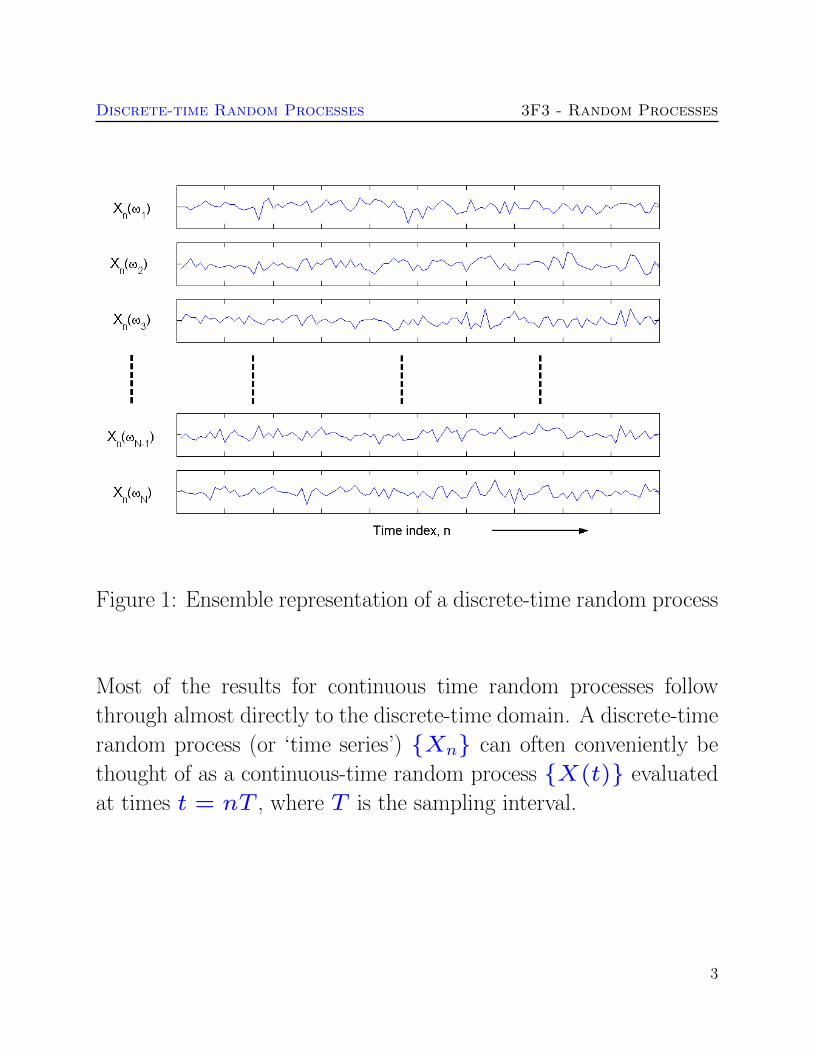
Discrete-time Random Processes 3F3 - Random Processes
Figure 1 Ensemble representation of a discrete-time random process
Most of the results for continuous time random processes follow
through almost directly to the discrete-time domain A discrete-time
random process (or lsquotime seriesrsquo) Xn can often conveniently be
thought of as a continuous-time random process X(t) evaluated
at times t = nT where T is the sampling interval
3
Discrete-time Random Processes 3F3 - Random Processes
Example the harmonic process
bull The harmonic process is important in a number of applications
including radar sonar speech and audio modelling An example
of a real-valued harmonic process is the random phase sinusoid
bull Here the signals we wish to describe are in the form of
sine-waves with known amplitude A and frequency Ω0 The
phase however is unknown and random which could
correspond to an unknown delay in a system for example
bull We can express this as a random process in the following form
xn = A sin(nΩ0 + φ)
Here A and Ω0 are fixed constants and φ is a random variable
having a uniform probability distribution over the range minusπ to
+π
f(φ) =
1(2π) minusπ lt φ le +π
0 otherwise
A selection of members of the ensemble is shown in the figure
4
Discrete-time Random Processes 3F3 - Random Processes
Figure 2 A few members of the random phase sine ensemble
A = 1 Ω0 = 0025
5
Discrete-time Random Processes 3F3 - Random Processes
Correlation functions
bull The mean of a random process Xn is defined as E[Xn] and
the autocorrelation function as
rXX[nm] = E[XnXm]
Autocorrelation function of random process
bull The cross-correlation function between two processes Xnand Yn is
rXY [nm] = E[XnYm]
Cross-correlation function
6
Discrete-time Random Processes 3F3 - Random Processes
Stationarity
A stationary process has the same statistical characteristics
irrespective of shifts along the time axis To put it another
way an observer looking at the process from sampling time n1
would not be able to tell the difference in the statistical
characteristics of the process if he moved to a different time n2
This idea is formalised by considering the N th order density for
the process
fXn1 Xn2 XnN(xn1
xn2 xnN)
Nth order density function for a discrete-time random process
which is the joint probability density function for N arbitrarily
chosen time indices n1 n2 nN Since the probability
distribution of a random vector contains all the statistical
information about that random vector we should expect the
probability distribution to be unchanged if we shifted the time
axis any amount to the left or the right for a stationary signal
This is the idea behind strict-sense stationarity for a discrete
random process
7
Discrete-time Random Processes 3F3 - Random Processes
A random process is strict-sense stationary if for any finite c
N and n1 n2 nN
fXn1 Xn2 XnN(α1 α2 αN)
= fXn1+cXn2+c XnN+c(α1 α2 αN)
Strict-sense stationarity for a random process
Strict-sense stationarity is hard to prove for most systems In
this course we will typically use a less stringent condition which
is nevertheless very useful for practical analysis This is known
as wide-sense stationarity which only requires first and second
order moments (ie mean and autocorrelation function) to be
invariant to time shifts
8
Discrete-time Random Processes 3F3 - Random Processes
A random process is wide-sense stationary (WSS) if
1 micron = E[Xn] = micro (mean is constant)
2 rXX[nm] = rXX[mminus n] (autocorrelation function
depends only upon the difference between n and m)
3 The variance of the process is finite
E[(Xn minus micro)2] ltinfin
Wide-sense stationarity for a random process
Note that strict-sense stationarity plus finite variance
(condition 3) implies wide-sense stationarity but not vice
versa
9
Discrete-time Random Processes 3F3 - Random Processes
Example random phase sine-wave
Continuing with the same example we can calculate the mean
and autocorrelation functions and hence check for stationarity
The process was defined as
xn = A sin(nΩ0 + φ)
A and Ω0 are fixed constants and φ is a random variable
having a uniform probability distribution over the range minusπ to
+π
f(φ) =
1(2π) minusπ lt φ le +π
0 otherwise
10
Discrete-time Random Processes 3F3 - Random Processes
1 Mean
E[Xn] = E[A sin(nΩ0 + φ)]
= AE[sin(nΩ0 + φ)]
= A E[sin(nΩ0) cos(φ) + cos(nΩ0) sin(φ)]
= A sin(nΩ0)E[cos(φ)] + cos(nΩ0)E[sin(φ)]
= 0
since E[cos(φ)] = E[sin(φ)] = 0 under the assumed
uniform distribution f(φ)
11
Discrete-time Random Processes 3F3 - Random Processes
2 Autocorrelation
rXX[nm]
= E[Xn Xm]
= E[A sin(nΩ0 + φ)A sin(mΩ0 + φ)]
= 05A2 E [cos[(nminusm)Ω0]minus cos[(n+m)Ω0 + 2φ]]
= 05A2cos[(nminusm)Ω0]minus E [cos[(n+m)Ω0 + 2φ]]
= 05A2cos[(nminusm)Ω0]
Hence the process satisfies the three criteria for wide sense
stationarity
12
Discrete-time Random Processes 3F3 - Random Processes
13
Discrete-time Random Processes 3F3 - Random Processes
Power spectra
For a wide-sense stationary random process Xn the power
spectrum is defined as the discrete-time Fourier transform
(DTFT) of the discrete autocorrelation function
SX(ejΩ
) =
infinsumm=minusinfin
rXX[m] eminusjmΩ
(1)
Power spectrum for a random process
where Ω = ωT is used for convenience
The autocorrelation function can thus be found from the power
spectrum by inverting the transform using the inverse DTFT
rXX[m] =1
2π
int π
minusπSX(e
jΩ) e
jmΩdΩ (2)
Autocorrelation function from power spectrum
14
Discrete-time Random Processes 3F3 - Random Processes
The power spectrum is a real positive even and periodic
function of frequency
The power spectrum can be interpreted as a density spectrum in
the sense that the mean-squared signal value at the output of an
ideal band-pass filter with lower and upper cut-off frequencies of
ωl and ωu is given by
1
π
int ωuT
ωlT
SX(ejΩ
) dΩ
Here we have assumed that the signal and the filter are real and
hence we add together the powers at negative and positive
frequencies
15
Discrete-time Random Processes 3F3 - Random Processes
Example power spectrum
The autocorrelation function for the random phase sine-wave
was previously obtained as
rXX[m] = 05A2cos[mΩ0]
Hence the power spectrum is obtained as
SX(ejΩ
) =
infinsumm=minusinfin
rXX[m] eminusjmΩ
=
infinsumm=minusinfin
05A2cos[mΩ0] e
minusjmΩ
= 025A2
timesinfinsum
m=minusinfin(exp(jmΩ0) + exp(minusjmΩ0)) e
minusjmΩ
= 05πA2
timesinfinsum
m=minusinfinδ(Ωminus Ω0 minus 2mπ)
+ δ(Ω + Ω0 minus 2mπ)
where Ω = ωT is once again used for shorthand
16
Discrete-time Random Processes 3F3 - Random Processes
Figure 3 Power spectrum of harmonic process
17
Discrete-time Random Processes 3F3 - Random Processes
White noise
White noise is defined in terms of its auto-covariance function
A wide sense stationary process is termed white noise if
cXX[m] = E[(Xn minus micro)(Xn+m minus micro)] = σ2Xδ[m]
where δ[m] is the discrete impulse function
δ[m] =
1 m = 0
0 otherwise
σ2X = E[(Xn minus micro)2] is the variance of the process If micro = 0
then σ2X is the mean-squared value of the process which we
will sometimes refer to as the lsquopowerrsquo
The power spectrum of zero mean white noise is
SX(ejωT
) =infinsum
m=minusinfinrXX[m] e
minusjmΩ
= σ2X
ie flat across all frequencies
18
Discrete-time Random Processes 3F3 - Random Processes
Example white Gaussian noise (WGN)
There are many ways to generate white noise processes all
having the property
cXX[m] = E[(Xn minus micro)(Xn+m minus micro)] = σ2Xδ[m]
The ensemble illustrated earlier in Fig was the zero-mean
Gaussian white noise process In this process the values Xn
are drawn independently from a Gaussian distribution with
mean 0 and variance σ2X
The N th order pdf for the Gaussian white noise process is
fXn1 Xn2 XnN(α1 α2 αN)
=Nprodi=1
N (αi|0 σ2X)
where
N (α|micro σ2) =
1radic
2πσ2exp
(minus
1
2σ2(xminus micro)
2
)is the univariate normal pdf
19
Discrete-time Random Processes 3F3 - Random Processes
We can immediately see that the Gaussian white noise process
is Strict sense stationary since
fXn1 Xn2 XnN(α1 α2 αN)
=Nprodi=1
N (αi|0 σ2X)
= fXn1+cXn2+c XnN+c (α1 α2 αN)
20
Discrete-time Random Processes 3F3 - Random Processes
21
Discrete-time Random Processes 3F3 - Random Processes
Linear systems and random processes
Figure 4 Linear system
When a wide-sense stationary discrete random process Xn is
passed through a stable linear time invariant (LTI) system with
22
Discrete-time Random Processes 3F3 - Random Processes
digital impulse response hn the output process Yn ie
yn =+infinsum
k=minusinfin
hk xnminusk = xn lowast hn
is also wide-sense stationary
23
Discrete-time Random Processes 3F3 - Random Processes
We can express the output correlation functions and power
spectra in terms of the input statistics and the LTI system
rXY [k] =E[Xn Yn+k] =
infinsuml=minusinfin
hl rXX[k minus l] = hk lowast rXX[k] (3)
Cross-correlation function at the output of a LTI system
rY Y [l] = E[Yn Yn+l]
infinsumk=minusinfin
infinsumi=minusinfin
hk hi rXX[l + iminus k] = hl lowast hminusl lowast rXX[l]
(4)
Autocorrelation function at the output of a LTI system
24
Discrete-time Random Processes 3F3 - Random Processes
Note these are convolutions as in the continuous-time case
This is easily remembered through the following figure
25
Discrete-time Random Processes 3F3 - Random Processes
Figure 5 Linear system - correlation functions
Taking DTFT of both sides of (4)
SY (ejωT
) = |H(ejωT
)|2SX(ejωT
) (5)
26
Discrete-time Random Processes 3F3 - Random Processes
Power spectrum at the output of a LTI system
27
Discrete-time Random Processes 3F3 - Random Processes
Example Filtering white noise
Suppose we filter a zero mean white noise process Xn with a first
order finite impulse response (FIR) filter
yn =1sum
m=0
bm xnminusm or Y (z) = (b0 + b1zminus1
)X(z)
with b0 = 1 b1 = 09 This an example of a moving average
(MA) process
The impulse response of this causal filter is
hn = b0 b1 0 0
The autocorrelation function of Yn is obtained as
rY Y [l] = E[Yn Yn+l] = hl lowast hminusl lowast rXX[l] (6)
This convolution can be performed directly However it is more
straightforward in the frequency domain
The frequency response of the filter is
H(ejΩ
) = b0 + b1eminusjΩ
28
Discrete-time Random Processes 3F3 - Random Processes
The power spectrum of Xn (white noise) is
SX(ejΩ
) = σ2X
Hence the power spectrum of Yn is
SY (ejΩ
) = |H(ejΩ
)|2SX(ejΩ
)
= |b0 + b1eminusjΩ|2σ2
X
= (b0b1e+jΩ
+ (b20 + b
21) + b0b1e
minusjΩ)σ
2X
as shown in the figure overleaf Comparing this expression with the
DTFT of rY Y [m]
SY (ejΩ
) =
infinsumm=minusinfin
rY Y [m] eminusjmΩ
we can identify non-zero terms in the summation only when m =
minus1 0+1 as follows
rY Y [minus1] = σ2Xb0b1 rY Y [0] = σ
2X(b
20 + b
21)
rY Y [1] = σ2Xb0b1
29
Discrete-time Random Processes 3F3 - Random Processes
Figure 6 Power spectrum of filtered white noise
30
Discrete-time Random Processes 3F3 - Random Processes
Ergodic Random processes
bull For an Ergodic random process we can estimate expectations
by performing time-averaging on a single sample function eg
micro = E[Xn] = limNrarrinfin
1
N
Nminus1sumn=0
xn (Mean ergodic)
rXX[k] = limNrarrinfin
1
N
Nminus1sumn=0
xnxn+k (Correlation ergodic) (7)
bull As in the continuous-time case these formulae allow us to make
the following estimates for lsquosufficientlyrsquo large N
micro = E[Xn] asymp1
N
Nminus1sumn=0
xn (Mean ergodic)
rXX[k] asymp1
N
Nminus1sumn=0
xnxn+k (Correlation ergodic) (8)
Note however that this is implemented with a simple computer
code loop in discrete-time unlike the continuous-time case
which requires an approximate integrator circuit
Under what conditions is a random process ergodic
31
Discrete-time Random Processes 3F3 - Random Processes
bull It is hard in general to determine whether a given process is
ergodic
bull A necessary and sufficient condition for mean ergodicity is given
by
limNrarrinfin
1
N
Nminus1sumk=0
cXX[k] = 0
where cXX is the autocovariance function
cXX[k] = E[(Xn minus micro)(Xn+k minus micro)]
and micro = E[Xn]
bull A simpler sufficient condition for mean ergodiciy is that
cXX[0] ltinfin and
limNrarrinfin
cXX[N ] = 0
bull Correlation ergodicity can be studied by extensions of the above
theorems We will not require the details here
bull Unless otherwise stated we will always assume that the signals
we encounter are both wide-sense stationary and ergodic
Although neither of these will always be true it will usually be
acceptable to assume so in practice
32
Discrete-time Random Processes 3F3 - Random Processes
Example
Consider the very simple lsquodc levelrsquo random process
Xn = A
where A is a random variable having the standard (ie mean zero
variance=1) Gaussian distribution
f(A) = N (A|0 1)
The mean of the random process is
E[Xn] =
int infinminusinfin
xn(a)f(a)da =
int infinminusinfin
af(a)da = 0
Now consider a random sample function measured from the random
process say
xt = a0
The mean value of this particular sample function is E[a0] = a0
Since in general a0 6= 0 the process is clearly not mean ergodic
33
Check this using the mean ergodic theorem The autocovariance
function is
cXX[k] = E[(Xn minus micro)(Xn+k minus micro)]
= E[XnXn+k] = E[A2] = 1
Now
limNrarrinfin
1
N
Nminus1sumk=0
cXX[k] = (1timesN)N = 1 6= 0
Hence the theorem confirms our finding that the process is not
ergodic in the mean
While this example highlights a possible pitfall in assuming
ergodicity most of the processes we deal with will however be
ergodic see examples paper for the random phase sine-wave and
the white noise processes
Comment Complex-valued processes
The above theory is easily extended to complex valued processes
Xn = XRen +jXIm
n in which case the autocorrelation function
is defined as
rXX[k] = E[XlowastnXn+k]
Revision Continuous time random processes
Figure 7 Ensemble representation of a random process
bull A random process is an ensemble of functions X(t) ω representingthe set of all possible waveforms that we might observe for that process
[NB ω is identical to the random variable α in the 3F1 notes]
ω is a random variable with its own probability distribution Pω whichdetermines randomly which waveform X(t ω) is observed ω may becontinuous- or discrete-valued
As before we will often omit ω and refer simply to random processX(t)
bull The mean of a random process is defined as micro(t) = E[X(t)] and theautocorrelation function as rXX [t1 t2] = E[X(t1)X(t2)] Theproperties of expectation allow us to calculate these in (at least) twoways
micro(t) = E[X(t1)]
=
intxx fX(t)(x) dx
=
intωX(t ω) fω(ω)dω
rXX(t1 t2) = E[X(t1)X(t2)]
=
intx1
intx2
x1x2 fX(t1)X(t2)(x1 x2) dx1dx2
=
intωX(t1 ω)X(t2 ω)fω(ω)dω
ie directly in terms of the density functions for X(t) or indirectly interms of the density function for ω
bull A wide-sense stationary (WSS) process X(t) is defined such that itsmean is a constant and rXX(t1 t2) depends only upon the differenceτ = t2 minus t1 ie
E[X(t)] = micro rXX(τ) = E[X(t)X(t+ τ)] (9)
[Wide-sense stationarity is also referred to as lsquoweak stationarityrsquo]
bull The Power Spectrum or Spectral Density of a WSS random process isdefined as the Fourier Transform of rXX(τ)
SX(ω) =
int infinminusinfin
rXX(τ) eminusjωτ
dτ (10)
bull For an Ergodic random process we can estimate expectations byperforming time-averaging on a single sample function eg
micro = E[X(t)] = limDrarrinfin
1
2D
int +D
minusDx(t)dt
rXX(τ) = limDrarrinfin
1
2D
int +D
minusDx(t)x(t+ τ)dt
Therefore for ergodic random processes we can make estimates forthese quantities by integrating over some suitably large (but finite) timeinterval 2D eg
E[X(t)] asymp1
2D
int +D
minusDx(t)dt
rXX(τ) asymp1
2D
int +D
minusDx(t)x(t+ τ)dt
where x(t) is a waveform measured at random from the process
Section 2 Optimal Filtering
Parts of this section and Section 3 are adapted from material kindly
supplied by Prof Peter Rayner
bull Optimal filtering is an area in which we design filters that are
optimally adapted to the statistical characteristics of a random
process As such the area can be seen as a combination of
standard filter design for deterministic signals with the random
process theory of the previous section
bull This remarkable area was pioneered in the 1940rsquos by Norbert
Wiener who designed methods for optimal estimation of a
signal measured in noise Specifically consider the system in the
figure below
Figure 8 The general Wiener filtering problem
bull A desired signal dn is observed in noise vn
xn = dn + vn
bull Wiener showed how to design a linear filter which would
optimally estimate dn given just the noisy observations xn and
some assumptions about the statistics of the random signal and
noise processes This class of filters the Wiener filter forms
the basis of many fundamental signal processing applications
bull Typical applications include
Noise reduction eg for speech and music signals
Prediction of future values of a signal eg in finance
Noise cancellation eg for aircraft cockpit noise
Deconvolution eg removal of room acoustics
(dereverberation) or echo cancellation in telephony
bull The Wiener filter is a very powerful tool However it is only the
optimal linear estimator for stationary signals The Kalman
filter offers an extension for non-stationary signals via state
space models In cases where a linear filter is still not good
enough non-linear filtering techniques can be adopted See 4th
year Signal Processing and Control modules for more advanced
topics in these areas
The Discrete-time Wiener Filter
In a minor abuse of notation and following standard conventions
we will refer to both random variables and their possible values in
lower-case symbols as this should cause no ambiguity for this section
of work
Figure 9 Wiener Filter
bull In the most general case we can filter the observed signal xnwith an Infinite impulse response (IIR) filter having a
non-causal impulse response hp
hp p = minusinfin minus1 0 1 2 infin (11)
bull We filter the observed noisy signal using the filter hp to
obtain an estimate dn of the desired signal
dn =infinsum
p=minusinfinhp xnminusp (12)
bull Since both dn and xn are drawn from random processes dnand xn we can only measure performance of the filter in
terms of expectations The criterion adopted for Wiener
filtering is the mean-squared error (MSE) criterion First
form the error signal εn
εn = dn minus dn = dn minusinfinsum
p=minusinfinhp xnminusp
The mean-squared error (MSE) is then defined as
J = E[ε2n] (13)
bull The Wiener filter minimises J with respect to the filter
coefficients hp
Derivation of Wiener filter
The Wiener filter assumes that xn and dn are jointly wide-
sense stationary This means that the means of both processes
are constant and all autocorrelation functionscross-correlation
functions (eg rxd[nm]) depend only on the time differencemminusnbetween data points
The expected error (13) may be minimised with respect to the
impulse response values hq A sufficient condition for a minimum
is
partJ
parthq=partE[ε2
n]
parthq= E
[partε2
n
parthq
]= E
[2εn
partεn
parthq
]= 0
for each q isin minusinfin minus1 0 1 2 infin
The term partεnparthq
is then calculated as
partεn
parthq=
part
parthq
dn minusinfinsum
p=minusinfinhp xnminusp
= minusxnminusq
and hence the coefficients must satisfy
E [εn xnminusq] = 0 minusinfin lt q lt +infin (14)
This is known as the orthogonality principle since two random
variables X and Y are termed orthogonal if
E[XY ] = 0
Now substituting for εn in (14) gives
E [εn xnminusq] = E
dn minus infinsump=minusinfin
hp xnminusp
xnminusq
= E [dn xnminusq]minus
infinsump=minusinfin
hp E [xnminusq xnminusp]
= rxd[q]minusinfinsum
p=minusinfinhp rxx[q minus p]
= 0
Hence rearranging the solution must satisfy
infinsump=minusinfin
hp rxx[q minus p] = rxd[q] minusinfin lt q lt +infin (15)
This is known as the Wiener-Hopf equations
The Wiener-Hopf equations involve an infinite number of unknowns
hq The simplest way to solve this is in the frequency domain First
note that the Wiener-Hopf equations can be rewritten as a discrete-
time convolution
hq lowast rxx[q] = rxd[q] minusinfin lt q lt +infin (16)
Taking discrete-time Fourier transforms (DTFT) of both sides
H(ejΩ
)Sx(ejΩ) = Sxd(ejΩ)
where Sxd(ejΩ) the DTFT of rxd[q] is defined as the cross-power
spectrum of d and x
Hence rearranging
H(ejΩ
) =Sxd(ejΩ)
Sx(ejΩ)(17)
Frequency domain Wiener filter
Mean-squared error for the optimal filter
The previous equations show how to calculate the optimal filter for
a given problem They donrsquot however tell us how well that optimal
filter performs This can be assessed from the mean-squared error
value of the optimal filter
J = E[ε2n] = E[εn(dn minus
infinsump=minusinfin
hp xnminusp)]
= E[εn dn]minusinfinsum
p=minusinfinhpE[εn xnminusp]
The expectation on the right is zero however for the optimal filter
by the orthogonality condition (14) so the minimum error is
Jmin = E[εn dn]
= E[(dn minusinfinsum
p=minusinfinhp xnminusp) dn]
= rdd[0]minusinfinsum
p=minusinfinhp rxd[p]
Important Special Case Uncorrelated Signal and Noise Processes
An important sub-class of the Wiener filter which also gives
considerable insight into filter behaviour can be gained by
considering the case where the desired signal process dn is
uncorrelated with the noise process vn ie
rdv[k] = E[dnvn+k] = 0 minusinfin lt k lt +infin
Consider the implications of this fact on the correlation functions
required in the Wiener-Hopf equations
infinsump=minusinfin
hp rxx[q minus p] = rxd[q] minusinfin lt q lt +infin
1 rxd
rxd[q] = E[xndn+q] = E[(dn + vn)dn+q] (18)
= E[dndn+q] + E[vndn+q] = rdd[q] (19)
since dn and vn are uncorrelated
Hence taking DTFT of both sides
Sxd(ejΩ) = Sd(ejΩ)
2 rxx
rxx[q] = E[xnxn+q] = E[(dn + vn)(dn+q + vn+q)]
= E[dndn+q] + E[vnvn+q] + E[dnvn+q] + E[vndn+q]
= E[dndn+q] + E[vnvn+q] = rdd[q] + rvv[q]
Hence
Sx(ejΩ) = Sd(ejΩ) + Sv(ejΩ)
Thus the Wiener filter becomes
H(ejΩ
) =Sd(ejΩ)
Sd(ejΩ) + Sv(ejΩ)
From this it can be seen that the behaviour of the filter is intuitively
reasonable in that at those frequencies where the noise power
spectrum Sv(ejΩ) is small the gain of the filter tends to unity
whereas the gain tends to a small value at those frequencies where the
noise spectrum is significantly larger than the desired signal power
spectrum Sd(ejΩ)
Example AR Process
An autoregressive process Dn of order 1 (see section 3) has power
spectrum
SD(ejΩ
) =σ2e
(1minus a1eminusjΩ)(1minus a1ejΩ)
Suppose the process is observed in zero mean white noise with
variance σ2v which is uncorrelated with Dn
xn = dn + vn
Design the Wiener filter for estimation of dn
Since the noise and desired signal are uncorrelated we can use the
form of Wiener filter from the previous page Substituting in the
various terms and rearranging its frequency response is
H(ejΩ
) =σ2e
σ2e + σ2
v(1minus a1eminusjΩ)(1minus a1ejΩ)
The impulse response of the filter can be found by inverse Fourier
transforming the frequency response This is studied in the examples
paper
The FIR Wiener filter
Note that in general the Wiener filter given by equation (17) is
non-causal and hence physically unrealisable in that the impulse
response hp is defined for values of p less than 0 Here we consider a
practical alternative in which a causal FIR Wiener filter is developed
In the FIR case the signal estimate is formed as
dn =
Pminus1sump=0
hp xnminusp (20)
and we minimise as before the objective function
J = E[(dn minus dn)2]
The filter derivation proceeds as before leading to an orthogonality
principle
E [εn xnminusq] = 0 q = 0 P minus 1 (21)
and Wiener-Hopf equations as follows
Pminus1sump=0
hp rxx[q minus p] = rxd[q] q = 0 1 P minus 1
(22)
The above equations may be written in matrix form as
Rxh = rxd
where
h =
h0
h1
hPminus1
rxd =
rxd[0]
rxd[1]
rxd[P minus 1]
and
Rx =
rxx[0] rxx[1] middot middot middot rxx[P minus 1]
rxx[1] rxx[0] rxx[P minus 2]
rxx[P minus 1] rxx[P minus 2] middot middot middot rxx[0]
Rx is known as the correlation matrix
Note that rxx[k] = rxx[minusk] so that the correlation matrix Rx
is symmetric and has constant diagonals (a symmetric Toeplitz
matrix)
The coefficient vector can be found by matrix inversion
h = Rxminus1
rxd (23)
This is the FIR Wiener filter and as for the general Wiener filter it
requires a-priori knowledge of the autocorrelation matrix Rx of the
input process xn and the cross-correlation rxd between the input
xn and the desired signal process dn
As before the minimum mean-squared error is given by
Jmin = E[εn dn]
= E[(dn minusPminus1sump=0
hp xnminusp) dn]
= rdd[0]minusPminus1sump=0
hp rxd[p]
= rdd[0]minus rTxdh = rdd[0]minus r
TxdRx
minus1rxd
Case Study Audio Noise Reduction
bull Consider a section of acoustic waveform (music voice ) dnthat is corrupted by additive noise vn
xn = dn + vn
bull We could try and noise reduce the signal using the FIR Wiener
filter
bull Assume that the section of data is wide-sense stationary and
ergodic (approx true for a short segment around 140 s)
Assume also that the noise is white and uncorrelated with the
audio signal - with variance σ2v ie
rvv[k] = σ2vδ[k]
Discrete-time Random Processes 3F3 - Random Processes
Example the harmonic process
bull The harmonic process is important in a number of applications
including radar sonar speech and audio modelling An example
of a real-valued harmonic process is the random phase sinusoid
bull Here the signals we wish to describe are in the form of
sine-waves with known amplitude A and frequency Ω0 The
phase however is unknown and random which could
correspond to an unknown delay in a system for example
bull We can express this as a random process in the following form
xn = A sin(nΩ0 + φ)
Here A and Ω0 are fixed constants and φ is a random variable
having a uniform probability distribution over the range minusπ to
+π
f(φ) =
1(2π) minusπ lt φ le +π
0 otherwise
A selection of members of the ensemble is shown in the figure
4
Discrete-time Random Processes 3F3 - Random Processes
Figure 2 A few members of the random phase sine ensemble
A = 1 Ω0 = 0025
5
Discrete-time Random Processes 3F3 - Random Processes
Correlation functions
bull The mean of a random process Xn is defined as E[Xn] and
the autocorrelation function as
rXX[nm] = E[XnXm]
Autocorrelation function of random process
bull The cross-correlation function between two processes Xnand Yn is
rXY [nm] = E[XnYm]
Cross-correlation function
6
Discrete-time Random Processes 3F3 - Random Processes
Stationarity
A stationary process has the same statistical characteristics
irrespective of shifts along the time axis To put it another
way an observer looking at the process from sampling time n1
would not be able to tell the difference in the statistical
characteristics of the process if he moved to a different time n2
This idea is formalised by considering the N th order density for
the process
fXn1 Xn2 XnN(xn1
xn2 xnN)
Nth order density function for a discrete-time random process
which is the joint probability density function for N arbitrarily
chosen time indices n1 n2 nN Since the probability
distribution of a random vector contains all the statistical
information about that random vector we should expect the
probability distribution to be unchanged if we shifted the time
axis any amount to the left or the right for a stationary signal
This is the idea behind strict-sense stationarity for a discrete
random process
7
Discrete-time Random Processes 3F3 - Random Processes
A random process is strict-sense stationary if for any finite c
N and n1 n2 nN
fXn1 Xn2 XnN(α1 α2 αN)
= fXn1+cXn2+c XnN+c(α1 α2 αN)
Strict-sense stationarity for a random process
Strict-sense stationarity is hard to prove for most systems In
this course we will typically use a less stringent condition which
is nevertheless very useful for practical analysis This is known
as wide-sense stationarity which only requires first and second
order moments (ie mean and autocorrelation function) to be
invariant to time shifts
8
Discrete-time Random Processes 3F3 - Random Processes
A random process is wide-sense stationary (WSS) if
1 micron = E[Xn] = micro (mean is constant)
2 rXX[nm] = rXX[mminus n] (autocorrelation function
depends only upon the difference between n and m)
3 The variance of the process is finite
E[(Xn minus micro)2] ltinfin
Wide-sense stationarity for a random process
Note that strict-sense stationarity plus finite variance
(condition 3) implies wide-sense stationarity but not vice
versa
9
Discrete-time Random Processes 3F3 - Random Processes
Example random phase sine-wave
Continuing with the same example we can calculate the mean
and autocorrelation functions and hence check for stationarity
The process was defined as
xn = A sin(nΩ0 + φ)
A and Ω0 are fixed constants and φ is a random variable
having a uniform probability distribution over the range minusπ to
+π
f(φ) =
1(2π) minusπ lt φ le +π
0 otherwise
10
Discrete-time Random Processes 3F3 - Random Processes
1 Mean
E[Xn] = E[A sin(nΩ0 + φ)]
= AE[sin(nΩ0 + φ)]
= A E[sin(nΩ0) cos(φ) + cos(nΩ0) sin(φ)]
= A sin(nΩ0)E[cos(φ)] + cos(nΩ0)E[sin(φ)]
= 0
since E[cos(φ)] = E[sin(φ)] = 0 under the assumed
uniform distribution f(φ)
11
Discrete-time Random Processes 3F3 - Random Processes
2 Autocorrelation
rXX[nm]
= E[Xn Xm]
= E[A sin(nΩ0 + φ)A sin(mΩ0 + φ)]
= 05A2 E [cos[(nminusm)Ω0]minus cos[(n+m)Ω0 + 2φ]]
= 05A2cos[(nminusm)Ω0]minus E [cos[(n+m)Ω0 + 2φ]]
= 05A2cos[(nminusm)Ω0]
Hence the process satisfies the three criteria for wide sense
stationarity
12
Discrete-time Random Processes 3F3 - Random Processes
13
Discrete-time Random Processes 3F3 - Random Processes
Power spectra
For a wide-sense stationary random process Xn the power
spectrum is defined as the discrete-time Fourier transform
(DTFT) of the discrete autocorrelation function
SX(ejΩ
) =
infinsumm=minusinfin
rXX[m] eminusjmΩ
(1)
Power spectrum for a random process
where Ω = ωT is used for convenience
The autocorrelation function can thus be found from the power
spectrum by inverting the transform using the inverse DTFT
rXX[m] =1
2π
int π
minusπSX(e
jΩ) e
jmΩdΩ (2)
Autocorrelation function from power spectrum
14
Discrete-time Random Processes 3F3 - Random Processes
The power spectrum is a real positive even and periodic
function of frequency
The power spectrum can be interpreted as a density spectrum in
the sense that the mean-squared signal value at the output of an
ideal band-pass filter with lower and upper cut-off frequencies of
ωl and ωu is given by
1
π
int ωuT
ωlT
SX(ejΩ
) dΩ
Here we have assumed that the signal and the filter are real and
hence we add together the powers at negative and positive
frequencies
15
Discrete-time Random Processes 3F3 - Random Processes
Example power spectrum
The autocorrelation function for the random phase sine-wave
was previously obtained as
rXX[m] = 05A2cos[mΩ0]
Hence the power spectrum is obtained as
SX(ejΩ
) =
infinsumm=minusinfin
rXX[m] eminusjmΩ
=
infinsumm=minusinfin
05A2cos[mΩ0] e
minusjmΩ
= 025A2
timesinfinsum
m=minusinfin(exp(jmΩ0) + exp(minusjmΩ0)) e
minusjmΩ
= 05πA2
timesinfinsum
m=minusinfinδ(Ωminus Ω0 minus 2mπ)
+ δ(Ω + Ω0 minus 2mπ)
where Ω = ωT is once again used for shorthand
16
Discrete-time Random Processes 3F3 - Random Processes
Figure 3 Power spectrum of harmonic process
17
Discrete-time Random Processes 3F3 - Random Processes
White noise
White noise is defined in terms of its auto-covariance function
A wide sense stationary process is termed white noise if
cXX[m] = E[(Xn minus micro)(Xn+m minus micro)] = σ2Xδ[m]
where δ[m] is the discrete impulse function
δ[m] =
1 m = 0
0 otherwise
σ2X = E[(Xn minus micro)2] is the variance of the process If micro = 0
then σ2X is the mean-squared value of the process which we
will sometimes refer to as the lsquopowerrsquo
The power spectrum of zero mean white noise is
SX(ejωT
) =infinsum
m=minusinfinrXX[m] e
minusjmΩ
= σ2X
ie flat across all frequencies
18
Discrete-time Random Processes 3F3 - Random Processes
Example white Gaussian noise (WGN)
There are many ways to generate white noise processes all
having the property
cXX[m] = E[(Xn minus micro)(Xn+m minus micro)] = σ2Xδ[m]
The ensemble illustrated earlier in Fig was the zero-mean
Gaussian white noise process In this process the values Xn
are drawn independently from a Gaussian distribution with
mean 0 and variance σ2X
The N th order pdf for the Gaussian white noise process is
fXn1 Xn2 XnN(α1 α2 αN)
=Nprodi=1
N (αi|0 σ2X)
where
N (α|micro σ2) =
1radic
2πσ2exp
(minus
1
2σ2(xminus micro)
2
)is the univariate normal pdf
19
Discrete-time Random Processes 3F3 - Random Processes
We can immediately see that the Gaussian white noise process
is Strict sense stationary since
fXn1 Xn2 XnN(α1 α2 αN)
=Nprodi=1
N (αi|0 σ2X)
= fXn1+cXn2+c XnN+c (α1 α2 αN)
20
Discrete-time Random Processes 3F3 - Random Processes
21
Discrete-time Random Processes 3F3 - Random Processes
Linear systems and random processes
Figure 4 Linear system
When a wide-sense stationary discrete random process Xn is
passed through a stable linear time invariant (LTI) system with
22
Discrete-time Random Processes 3F3 - Random Processes
digital impulse response hn the output process Yn ie
yn =+infinsum
k=minusinfin
hk xnminusk = xn lowast hn
is also wide-sense stationary
23
Discrete-time Random Processes 3F3 - Random Processes
We can express the output correlation functions and power
spectra in terms of the input statistics and the LTI system
rXY [k] =E[Xn Yn+k] =
infinsuml=minusinfin
hl rXX[k minus l] = hk lowast rXX[k] (3)
Cross-correlation function at the output of a LTI system
rY Y [l] = E[Yn Yn+l]
infinsumk=minusinfin
infinsumi=minusinfin
hk hi rXX[l + iminus k] = hl lowast hminusl lowast rXX[l]
(4)
Autocorrelation function at the output of a LTI system
24
Discrete-time Random Processes 3F3 - Random Processes
Note these are convolutions as in the continuous-time case
This is easily remembered through the following figure
25
Discrete-time Random Processes 3F3 - Random Processes
Figure 5 Linear system - correlation functions
Taking DTFT of both sides of (4)
SY (ejωT
) = |H(ejωT
)|2SX(ejωT
) (5)
26
Discrete-time Random Processes 3F3 - Random Processes
Power spectrum at the output of a LTI system
27
Discrete-time Random Processes 3F3 - Random Processes
Example Filtering white noise
Suppose we filter a zero mean white noise process Xn with a first
order finite impulse response (FIR) filter
yn =1sum
m=0
bm xnminusm or Y (z) = (b0 + b1zminus1
)X(z)
with b0 = 1 b1 = 09 This an example of a moving average
(MA) process
The impulse response of this causal filter is
hn = b0 b1 0 0
The autocorrelation function of Yn is obtained as
rY Y [l] = E[Yn Yn+l] = hl lowast hminusl lowast rXX[l] (6)
This convolution can be performed directly However it is more
straightforward in the frequency domain
The frequency response of the filter is
H(ejΩ
) = b0 + b1eminusjΩ
28
Discrete-time Random Processes 3F3 - Random Processes
The power spectrum of Xn (white noise) is
SX(ejΩ
) = σ2X
Hence the power spectrum of Yn is
SY (ejΩ
) = |H(ejΩ
)|2SX(ejΩ
)
= |b0 + b1eminusjΩ|2σ2
X
= (b0b1e+jΩ
+ (b20 + b
21) + b0b1e
minusjΩ)σ
2X
as shown in the figure overleaf Comparing this expression with the
DTFT of rY Y [m]
SY (ejΩ
) =
infinsumm=minusinfin
rY Y [m] eminusjmΩ
we can identify non-zero terms in the summation only when m =
minus1 0+1 as follows
rY Y [minus1] = σ2Xb0b1 rY Y [0] = σ
2X(b
20 + b
21)
rY Y [1] = σ2Xb0b1
29
Discrete-time Random Processes 3F3 - Random Processes
Figure 6 Power spectrum of filtered white noise
30
Discrete-time Random Processes 3F3 - Random Processes
Ergodic Random processes
bull For an Ergodic random process we can estimate expectations
by performing time-averaging on a single sample function eg
micro = E[Xn] = limNrarrinfin
1
N
Nminus1sumn=0
xn (Mean ergodic)
rXX[k] = limNrarrinfin
1
N
Nminus1sumn=0
xnxn+k (Correlation ergodic) (7)
bull As in the continuous-time case these formulae allow us to make
the following estimates for lsquosufficientlyrsquo large N
micro = E[Xn] asymp1
N
Nminus1sumn=0
xn (Mean ergodic)
rXX[k] asymp1
N
Nminus1sumn=0
xnxn+k (Correlation ergodic) (8)
Note however that this is implemented with a simple computer
code loop in discrete-time unlike the continuous-time case
which requires an approximate integrator circuit
Under what conditions is a random process ergodic
31
Discrete-time Random Processes 3F3 - Random Processes
bull It is hard in general to determine whether a given process is
ergodic
bull A necessary and sufficient condition for mean ergodicity is given
by
limNrarrinfin
1
N
Nminus1sumk=0
cXX[k] = 0
where cXX is the autocovariance function
cXX[k] = E[(Xn minus micro)(Xn+k minus micro)]
and micro = E[Xn]
bull A simpler sufficient condition for mean ergodiciy is that
cXX[0] ltinfin and
limNrarrinfin
cXX[N ] = 0
bull Correlation ergodicity can be studied by extensions of the above
theorems We will not require the details here
bull Unless otherwise stated we will always assume that the signals
we encounter are both wide-sense stationary and ergodic
Although neither of these will always be true it will usually be
acceptable to assume so in practice
32
Discrete-time Random Processes 3F3 - Random Processes
Example
Consider the very simple lsquodc levelrsquo random process
Xn = A
where A is a random variable having the standard (ie mean zero
variance=1) Gaussian distribution
f(A) = N (A|0 1)
The mean of the random process is
E[Xn] =
int infinminusinfin
xn(a)f(a)da =
int infinminusinfin
af(a)da = 0
Now consider a random sample function measured from the random
process say
xt = a0
The mean value of this particular sample function is E[a0] = a0
Since in general a0 6= 0 the process is clearly not mean ergodic
33
Check this using the mean ergodic theorem The autocovariance
function is
cXX[k] = E[(Xn minus micro)(Xn+k minus micro)]
= E[XnXn+k] = E[A2] = 1
Now
limNrarrinfin
1
N
Nminus1sumk=0
cXX[k] = (1timesN)N = 1 6= 0
Hence the theorem confirms our finding that the process is not
ergodic in the mean
While this example highlights a possible pitfall in assuming
ergodicity most of the processes we deal with will however be
ergodic see examples paper for the random phase sine-wave and
the white noise processes
Comment Complex-valued processes
The above theory is easily extended to complex valued processes
Xn = XRen +jXIm
n in which case the autocorrelation function
is defined as
rXX[k] = E[XlowastnXn+k]
Revision Continuous time random processes
Figure 7 Ensemble representation of a random process
bull A random process is an ensemble of functions X(t) ω representingthe set of all possible waveforms that we might observe for that process
[NB ω is identical to the random variable α in the 3F1 notes]
ω is a random variable with its own probability distribution Pω whichdetermines randomly which waveform X(t ω) is observed ω may becontinuous- or discrete-valued
As before we will often omit ω and refer simply to random processX(t)
bull The mean of a random process is defined as micro(t) = E[X(t)] and theautocorrelation function as rXX [t1 t2] = E[X(t1)X(t2)] Theproperties of expectation allow us to calculate these in (at least) twoways
micro(t) = E[X(t1)]
=
intxx fX(t)(x) dx
=
intωX(t ω) fω(ω)dω
rXX(t1 t2) = E[X(t1)X(t2)]
=
intx1
intx2
x1x2 fX(t1)X(t2)(x1 x2) dx1dx2
=
intωX(t1 ω)X(t2 ω)fω(ω)dω
ie directly in terms of the density functions for X(t) or indirectly interms of the density function for ω
bull A wide-sense stationary (WSS) process X(t) is defined such that itsmean is a constant and rXX(t1 t2) depends only upon the differenceτ = t2 minus t1 ie
E[X(t)] = micro rXX(τ) = E[X(t)X(t+ τ)] (9)
[Wide-sense stationarity is also referred to as lsquoweak stationarityrsquo]
bull The Power Spectrum or Spectral Density of a WSS random process isdefined as the Fourier Transform of rXX(τ)
SX(ω) =
int infinminusinfin
rXX(τ) eminusjωτ
dτ (10)
bull For an Ergodic random process we can estimate expectations byperforming time-averaging on a single sample function eg
micro = E[X(t)] = limDrarrinfin
1
2D
int +D
minusDx(t)dt
rXX(τ) = limDrarrinfin
1
2D
int +D
minusDx(t)x(t+ τ)dt
Therefore for ergodic random processes we can make estimates forthese quantities by integrating over some suitably large (but finite) timeinterval 2D eg
E[X(t)] asymp1
2D
int +D
minusDx(t)dt
rXX(τ) asymp1
2D
int +D
minusDx(t)x(t+ τ)dt
where x(t) is a waveform measured at random from the process
Section 2 Optimal Filtering
Parts of this section and Section 3 are adapted from material kindly
supplied by Prof Peter Rayner
bull Optimal filtering is an area in which we design filters that are
optimally adapted to the statistical characteristics of a random
process As such the area can be seen as a combination of
standard filter design for deterministic signals with the random
process theory of the previous section
bull This remarkable area was pioneered in the 1940rsquos by Norbert
Wiener who designed methods for optimal estimation of a
signal measured in noise Specifically consider the system in the
figure below
Figure 8 The general Wiener filtering problem
bull A desired signal dn is observed in noise vn
xn = dn + vn
bull Wiener showed how to design a linear filter which would
optimally estimate dn given just the noisy observations xn and
some assumptions about the statistics of the random signal and
noise processes This class of filters the Wiener filter forms
the basis of many fundamental signal processing applications
bull Typical applications include
Noise reduction eg for speech and music signals
Prediction of future values of a signal eg in finance
Noise cancellation eg for aircraft cockpit noise
Deconvolution eg removal of room acoustics
(dereverberation) or echo cancellation in telephony
bull The Wiener filter is a very powerful tool However it is only the
optimal linear estimator for stationary signals The Kalman
filter offers an extension for non-stationary signals via state
space models In cases where a linear filter is still not good
enough non-linear filtering techniques can be adopted See 4th
year Signal Processing and Control modules for more advanced
topics in these areas
The Discrete-time Wiener Filter
In a minor abuse of notation and following standard conventions
we will refer to both random variables and their possible values in
lower-case symbols as this should cause no ambiguity for this section
of work
Figure 9 Wiener Filter
bull In the most general case we can filter the observed signal xnwith an Infinite impulse response (IIR) filter having a
non-causal impulse response hp
hp p = minusinfin minus1 0 1 2 infin (11)
bull We filter the observed noisy signal using the filter hp to
obtain an estimate dn of the desired signal
dn =infinsum
p=minusinfinhp xnminusp (12)
bull Since both dn and xn are drawn from random processes dnand xn we can only measure performance of the filter in
terms of expectations The criterion adopted for Wiener
filtering is the mean-squared error (MSE) criterion First
form the error signal εn
εn = dn minus dn = dn minusinfinsum
p=minusinfinhp xnminusp
The mean-squared error (MSE) is then defined as
J = E[ε2n] (13)
bull The Wiener filter minimises J with respect to the filter
coefficients hp
Derivation of Wiener filter
The Wiener filter assumes that xn and dn are jointly wide-
sense stationary This means that the means of both processes
are constant and all autocorrelation functionscross-correlation
functions (eg rxd[nm]) depend only on the time differencemminusnbetween data points
The expected error (13) may be minimised with respect to the
impulse response values hq A sufficient condition for a minimum
is
partJ
parthq=partE[ε2
n]
parthq= E
[partε2
n
parthq
]= E
[2εn
partεn
parthq
]= 0
for each q isin minusinfin minus1 0 1 2 infin
The term partεnparthq
is then calculated as
partεn
parthq=
part
parthq
dn minusinfinsum
p=minusinfinhp xnminusp
= minusxnminusq
and hence the coefficients must satisfy
E [εn xnminusq] = 0 minusinfin lt q lt +infin (14)
This is known as the orthogonality principle since two random
variables X and Y are termed orthogonal if
E[XY ] = 0
Now substituting for εn in (14) gives
E [εn xnminusq] = E
dn minus infinsump=minusinfin
hp xnminusp
xnminusq
= E [dn xnminusq]minus
infinsump=minusinfin
hp E [xnminusq xnminusp]
= rxd[q]minusinfinsum
p=minusinfinhp rxx[q minus p]
= 0
Hence rearranging the solution must satisfy
infinsump=minusinfin
hp rxx[q minus p] = rxd[q] minusinfin lt q lt +infin (15)
This is known as the Wiener-Hopf equations
The Wiener-Hopf equations involve an infinite number of unknowns
hq The simplest way to solve this is in the frequency domain First
note that the Wiener-Hopf equations can be rewritten as a discrete-
time convolution
hq lowast rxx[q] = rxd[q] minusinfin lt q lt +infin (16)
Taking discrete-time Fourier transforms (DTFT) of both sides
H(ejΩ
)Sx(ejΩ) = Sxd(ejΩ)
where Sxd(ejΩ) the DTFT of rxd[q] is defined as the cross-power
spectrum of d and x
Hence rearranging
H(ejΩ
) =Sxd(ejΩ)
Sx(ejΩ)(17)
Frequency domain Wiener filter
Mean-squared error for the optimal filter
The previous equations show how to calculate the optimal filter for
a given problem They donrsquot however tell us how well that optimal
filter performs This can be assessed from the mean-squared error
value of the optimal filter
J = E[ε2n] = E[εn(dn minus
infinsump=minusinfin
hp xnminusp)]
= E[εn dn]minusinfinsum
p=minusinfinhpE[εn xnminusp]
The expectation on the right is zero however for the optimal filter
by the orthogonality condition (14) so the minimum error is
Jmin = E[εn dn]
= E[(dn minusinfinsum
p=minusinfinhp xnminusp) dn]
= rdd[0]minusinfinsum
p=minusinfinhp rxd[p]
Important Special Case Uncorrelated Signal and Noise Processes
An important sub-class of the Wiener filter which also gives
considerable insight into filter behaviour can be gained by
considering the case where the desired signal process dn is
uncorrelated with the noise process vn ie
rdv[k] = E[dnvn+k] = 0 minusinfin lt k lt +infin
Consider the implications of this fact on the correlation functions
required in the Wiener-Hopf equations
infinsump=minusinfin
hp rxx[q minus p] = rxd[q] minusinfin lt q lt +infin
1 rxd
rxd[q] = E[xndn+q] = E[(dn + vn)dn+q] (18)
= E[dndn+q] + E[vndn+q] = rdd[q] (19)
since dn and vn are uncorrelated
Hence taking DTFT of both sides
Sxd(ejΩ) = Sd(ejΩ)
2 rxx
rxx[q] = E[xnxn+q] = E[(dn + vn)(dn+q + vn+q)]
= E[dndn+q] + E[vnvn+q] + E[dnvn+q] + E[vndn+q]
= E[dndn+q] + E[vnvn+q] = rdd[q] + rvv[q]
Hence
Sx(ejΩ) = Sd(ejΩ) + Sv(ejΩ)
Thus the Wiener filter becomes
H(ejΩ
) =Sd(ejΩ)
Sd(ejΩ) + Sv(ejΩ)
From this it can be seen that the behaviour of the filter is intuitively
reasonable in that at those frequencies where the noise power
spectrum Sv(ejΩ) is small the gain of the filter tends to unity
whereas the gain tends to a small value at those frequencies where the
noise spectrum is significantly larger than the desired signal power
spectrum Sd(ejΩ)
Example AR Process
An autoregressive process Dn of order 1 (see section 3) has power
spectrum
SD(ejΩ
) =σ2e
(1minus a1eminusjΩ)(1minus a1ejΩ)
Suppose the process is observed in zero mean white noise with
variance σ2v which is uncorrelated with Dn
xn = dn + vn
Design the Wiener filter for estimation of dn
Since the noise and desired signal are uncorrelated we can use the
form of Wiener filter from the previous page Substituting in the
various terms and rearranging its frequency response is
H(ejΩ
) =σ2e
σ2e + σ2
v(1minus a1eminusjΩ)(1minus a1ejΩ)
The impulse response of the filter can be found by inverse Fourier
transforming the frequency response This is studied in the examples
paper
The FIR Wiener filter
Note that in general the Wiener filter given by equation (17) is
non-causal and hence physically unrealisable in that the impulse
response hp is defined for values of p less than 0 Here we consider a
practical alternative in which a causal FIR Wiener filter is developed
In the FIR case the signal estimate is formed as
dn =
Pminus1sump=0
hp xnminusp (20)
and we minimise as before the objective function
J = E[(dn minus dn)2]
The filter derivation proceeds as before leading to an orthogonality
principle
E [εn xnminusq] = 0 q = 0 P minus 1 (21)
and Wiener-Hopf equations as follows
Pminus1sump=0
hp rxx[q minus p] = rxd[q] q = 0 1 P minus 1
(22)
The above equations may be written in matrix form as
Rxh = rxd
where
h =
h0
h1
hPminus1
rxd =
rxd[0]
rxd[1]
rxd[P minus 1]
and
Rx =
rxx[0] rxx[1] middot middot middot rxx[P minus 1]
rxx[1] rxx[0] rxx[P minus 2]
rxx[P minus 1] rxx[P minus 2] middot middot middot rxx[0]
Rx is known as the correlation matrix
Note that rxx[k] = rxx[minusk] so that the correlation matrix Rx
is symmetric and has constant diagonals (a symmetric Toeplitz
matrix)
The coefficient vector can be found by matrix inversion
h = Rxminus1
rxd (23)
This is the FIR Wiener filter and as for the general Wiener filter it
requires a-priori knowledge of the autocorrelation matrix Rx of the
input process xn and the cross-correlation rxd between the input
xn and the desired signal process dn
As before the minimum mean-squared error is given by
Jmin = E[εn dn]
= E[(dn minusPminus1sump=0
hp xnminusp) dn]
= rdd[0]minusPminus1sump=0
hp rxd[p]
= rdd[0]minus rTxdh = rdd[0]minus r
TxdRx
minus1rxd
Case Study Audio Noise Reduction
bull Consider a section of acoustic waveform (music voice ) dnthat is corrupted by additive noise vn
xn = dn + vn
bull We could try and noise reduce the signal using the FIR Wiener
filter
bull Assume that the section of data is wide-sense stationary and
ergodic (approx true for a short segment around 140 s)
Assume also that the noise is white and uncorrelated with the
audio signal - with variance σ2v ie
rvv[k] = σ2vδ[k]

Discrete-time Random Processes 3F3 - Random Processes
Figure 2 A few members of the random phase sine ensemble
A = 1 Ω0 = 0025
5
Discrete-time Random Processes 3F3 - Random Processes
Correlation functions
bull The mean of a random process Xn is defined as E[Xn] and
the autocorrelation function as
rXX[nm] = E[XnXm]
Autocorrelation function of random process
bull The cross-correlation function between two processes Xnand Yn is
rXY [nm] = E[XnYm]
Cross-correlation function
6
Discrete-time Random Processes 3F3 - Random Processes
Stationarity
A stationary process has the same statistical characteristics
irrespective of shifts along the time axis To put it another
way an observer looking at the process from sampling time n1
would not be able to tell the difference in the statistical
characteristics of the process if he moved to a different time n2
This idea is formalised by considering the N th order density for
the process
fXn1 Xn2 XnN(xn1
xn2 xnN)
Nth order density function for a discrete-time random process
which is the joint probability density function for N arbitrarily
chosen time indices n1 n2 nN Since the probability
distribution of a random vector contains all the statistical
information about that random vector we should expect the
probability distribution to be unchanged if we shifted the time
axis any amount to the left or the right for a stationary signal
This is the idea behind strict-sense stationarity for a discrete
random process
7
Discrete-time Random Processes 3F3 - Random Processes
A random process is strict-sense stationary if for any finite c
N and n1 n2 nN
fXn1 Xn2 XnN(α1 α2 αN)
= fXn1+cXn2+c XnN+c(α1 α2 αN)
Strict-sense stationarity for a random process
Strict-sense stationarity is hard to prove for most systems In
this course we will typically use a less stringent condition which
is nevertheless very useful for practical analysis This is known
as wide-sense stationarity which only requires first and second
order moments (ie mean and autocorrelation function) to be
invariant to time shifts
8
Discrete-time Random Processes 3F3 - Random Processes
A random process is wide-sense stationary (WSS) if
1 micron = E[Xn] = micro (mean is constant)
2 rXX[nm] = rXX[mminus n] (autocorrelation function
depends only upon the difference between n and m)
3 The variance of the process is finite
E[(Xn minus micro)2] ltinfin
Wide-sense stationarity for a random process
Note that strict-sense stationarity plus finite variance
(condition 3) implies wide-sense stationarity but not vice
versa
9
Discrete-time Random Processes 3F3 - Random Processes
Example random phase sine-wave
Continuing with the same example we can calculate the mean
and autocorrelation functions and hence check for stationarity
The process was defined as
xn = A sin(nΩ0 + φ)
A and Ω0 are fixed constants and φ is a random variable
having a uniform probability distribution over the range minusπ to
+π
f(φ) =
1(2π) minusπ lt φ le +π
0 otherwise
10
Discrete-time Random Processes 3F3 - Random Processes
1 Mean
E[Xn] = E[A sin(nΩ0 + φ)]
= AE[sin(nΩ0 + φ)]
= A E[sin(nΩ0) cos(φ) + cos(nΩ0) sin(φ)]
= A sin(nΩ0)E[cos(φ)] + cos(nΩ0)E[sin(φ)]
= 0
since E[cos(φ)] = E[sin(φ)] = 0 under the assumed
uniform distribution f(φ)
11
Discrete-time Random Processes 3F3 - Random Processes
2 Autocorrelation
rXX[nm]
= E[Xn Xm]
= E[A sin(nΩ0 + φ)A sin(mΩ0 + φ)]
= 05A2 E [cos[(nminusm)Ω0]minus cos[(n+m)Ω0 + 2φ]]
= 05A2cos[(nminusm)Ω0]minus E [cos[(n+m)Ω0 + 2φ]]
= 05A2cos[(nminusm)Ω0]
Hence the process satisfies the three criteria for wide sense
stationarity
12
Discrete-time Random Processes 3F3 - Random Processes
13
Discrete-time Random Processes 3F3 - Random Processes
Power spectra
For a wide-sense stationary random process Xn the power
spectrum is defined as the discrete-time Fourier transform
(DTFT) of the discrete autocorrelation function
SX(ejΩ
) =
infinsumm=minusinfin
rXX[m] eminusjmΩ
(1)
Power spectrum for a random process
where Ω = ωT is used for convenience
The autocorrelation function can thus be found from the power
spectrum by inverting the transform using the inverse DTFT
rXX[m] =1
2π
int π
minusπSX(e
jΩ) e
jmΩdΩ (2)
Autocorrelation function from power spectrum
14
Discrete-time Random Processes 3F3 - Random Processes
The power spectrum is a real positive even and periodic
function of frequency
The power spectrum can be interpreted as a density spectrum in
the sense that the mean-squared signal value at the output of an
ideal band-pass filter with lower and upper cut-off frequencies of
ωl and ωu is given by
1
π
int ωuT
ωlT
SX(ejΩ
) dΩ
Here we have assumed that the signal and the filter are real and
hence we add together the powers at negative and positive
frequencies
15
Discrete-time Random Processes 3F3 - Random Processes
Example power spectrum
The autocorrelation function for the random phase sine-wave
was previously obtained as
rXX[m] = 05A2cos[mΩ0]
Hence the power spectrum is obtained as
SX(ejΩ
) =
infinsumm=minusinfin
rXX[m] eminusjmΩ
=
infinsumm=minusinfin
05A2cos[mΩ0] e
minusjmΩ
= 025A2
timesinfinsum
m=minusinfin(exp(jmΩ0) + exp(minusjmΩ0)) e
minusjmΩ
= 05πA2
timesinfinsum
m=minusinfinδ(Ωminus Ω0 minus 2mπ)
+ δ(Ω + Ω0 minus 2mπ)
where Ω = ωT is once again used for shorthand
16
Discrete-time Random Processes 3F3 - Random Processes
Figure 3 Power spectrum of harmonic process
17
Discrete-time Random Processes 3F3 - Random Processes
White noise
White noise is defined in terms of its auto-covariance function
A wide sense stationary process is termed white noise if
cXX[m] = E[(Xn minus micro)(Xn+m minus micro)] = σ2Xδ[m]
where δ[m] is the discrete impulse function
δ[m] =
1 m = 0
0 otherwise
σ2X = E[(Xn minus micro)2] is the variance of the process If micro = 0
then σ2X is the mean-squared value of the process which we
will sometimes refer to as the lsquopowerrsquo
The power spectrum of zero mean white noise is
SX(ejωT
) =infinsum
m=minusinfinrXX[m] e
minusjmΩ
= σ2X
ie flat across all frequencies
18
Discrete-time Random Processes 3F3 - Random Processes
Example white Gaussian noise (WGN)
There are many ways to generate white noise processes all
having the property
cXX[m] = E[(Xn minus micro)(Xn+m minus micro)] = σ2Xδ[m]
The ensemble illustrated earlier in Fig was the zero-mean
Gaussian white noise process In this process the values Xn
are drawn independently from a Gaussian distribution with
mean 0 and variance σ2X
The N th order pdf for the Gaussian white noise process is
fXn1 Xn2 XnN(α1 α2 αN)
=Nprodi=1
N (αi|0 σ2X)
where
N (α|micro σ2) =
1radic
2πσ2exp
(minus
1
2σ2(xminus micro)
2
)is the univariate normal pdf
19
Discrete-time Random Processes 3F3 - Random Processes
We can immediately see that the Gaussian white noise process
is Strict sense stationary since
fXn1 Xn2 XnN(α1 α2 αN)
=Nprodi=1
N (αi|0 σ2X)
= fXn1+cXn2+c XnN+c (α1 α2 αN)
20
Discrete-time Random Processes 3F3 - Random Processes
21
Discrete-time Random Processes 3F3 - Random Processes
Linear systems and random processes
Figure 4 Linear system
When a wide-sense stationary discrete random process Xn is
passed through a stable linear time invariant (LTI) system with
22
Discrete-time Random Processes 3F3 - Random Processes
digital impulse response hn the output process Yn ie
yn =+infinsum
k=minusinfin
hk xnminusk = xn lowast hn
is also wide-sense stationary
23
Discrete-time Random Processes 3F3 - Random Processes
We can express the output correlation functions and power
spectra in terms of the input statistics and the LTI system
rXY [k] =E[Xn Yn+k] =
infinsuml=minusinfin
hl rXX[k minus l] = hk lowast rXX[k] (3)
Cross-correlation function at the output of a LTI system
rY Y [l] = E[Yn Yn+l]
infinsumk=minusinfin
infinsumi=minusinfin
hk hi rXX[l + iminus k] = hl lowast hminusl lowast rXX[l]
(4)
Autocorrelation function at the output of a LTI system
24
Discrete-time Random Processes 3F3 - Random Processes
Note these are convolutions as in the continuous-time case
This is easily remembered through the following figure
25
Discrete-time Random Processes 3F3 - Random Processes
Figure 5 Linear system - correlation functions
Taking DTFT of both sides of (4)
SY (ejωT
) = |H(ejωT
)|2SX(ejωT
) (5)
26
Discrete-time Random Processes 3F3 - Random Processes
Power spectrum at the output of a LTI system
27
Discrete-time Random Processes 3F3 - Random Processes
Example Filtering white noise
Suppose we filter a zero mean white noise process Xn with a first
order finite impulse response (FIR) filter
yn =1sum
m=0
bm xnminusm or Y (z) = (b0 + b1zminus1
)X(z)
with b0 = 1 b1 = 09 This an example of a moving average
(MA) process
The impulse response of this causal filter is
hn = b0 b1 0 0
The autocorrelation function of Yn is obtained as
rY Y [l] = E[Yn Yn+l] = hl lowast hminusl lowast rXX[l] (6)
This convolution can be performed directly However it is more
straightforward in the frequency domain
The frequency response of the filter is
H(ejΩ
) = b0 + b1eminusjΩ
28
Discrete-time Random Processes 3F3 - Random Processes
The power spectrum of Xn (white noise) is
SX(ejΩ
) = σ2X
Hence the power spectrum of Yn is
SY (ejΩ
) = |H(ejΩ
)|2SX(ejΩ
)
= |b0 + b1eminusjΩ|2σ2
X
= (b0b1e+jΩ
+ (b20 + b
21) + b0b1e
minusjΩ)σ
2X
as shown in the figure overleaf Comparing this expression with the
DTFT of rY Y [m]
SY (ejΩ
) =
infinsumm=minusinfin
rY Y [m] eminusjmΩ
we can identify non-zero terms in the summation only when m =
minus1 0+1 as follows
rY Y [minus1] = σ2Xb0b1 rY Y [0] = σ
2X(b
20 + b
21)
rY Y [1] = σ2Xb0b1
29
Discrete-time Random Processes 3F3 - Random Processes
Figure 6 Power spectrum of filtered white noise
30
Discrete-time Random Processes 3F3 - Random Processes
Ergodic Random processes
bull For an Ergodic random process we can estimate expectations
by performing time-averaging on a single sample function eg
micro = E[Xn] = limNrarrinfin
1
N
Nminus1sumn=0
xn (Mean ergodic)
rXX[k] = limNrarrinfin
1
N
Nminus1sumn=0
xnxn+k (Correlation ergodic) (7)
bull As in the continuous-time case these formulae allow us to make
the following estimates for lsquosufficientlyrsquo large N
micro = E[Xn] asymp1
N
Nminus1sumn=0
xn (Mean ergodic)
rXX[k] asymp1
N
Nminus1sumn=0
xnxn+k (Correlation ergodic) (8)
Note however that this is implemented with a simple computer
code loop in discrete-time unlike the continuous-time case
which requires an approximate integrator circuit
Under what conditions is a random process ergodic
31
Discrete-time Random Processes 3F3 - Random Processes
bull It is hard in general to determine whether a given process is
ergodic
bull A necessary and sufficient condition for mean ergodicity is given
by
limNrarrinfin
1
N
Nminus1sumk=0
cXX[k] = 0
where cXX is the autocovariance function
cXX[k] = E[(Xn minus micro)(Xn+k minus micro)]
and micro = E[Xn]
bull A simpler sufficient condition for mean ergodiciy is that
cXX[0] ltinfin and
limNrarrinfin
cXX[N ] = 0
bull Correlation ergodicity can be studied by extensions of the above
theorems We will not require the details here
bull Unless otherwise stated we will always assume that the signals
we encounter are both wide-sense stationary and ergodic
Although neither of these will always be true it will usually be
acceptable to assume so in practice
32
Discrete-time Random Processes 3F3 - Random Processes
Example
Consider the very simple lsquodc levelrsquo random process
Xn = A
where A is a random variable having the standard (ie mean zero
variance=1) Gaussian distribution
f(A) = N (A|0 1)
The mean of the random process is
E[Xn] =
int infinminusinfin
xn(a)f(a)da =
int infinminusinfin
af(a)da = 0
Now consider a random sample function measured from the random
process say
xt = a0
The mean value of this particular sample function is E[a0] = a0
Since in general a0 6= 0 the process is clearly not mean ergodic
33
Check this using the mean ergodic theorem The autocovariance
function is
cXX[k] = E[(Xn minus micro)(Xn+k minus micro)]
= E[XnXn+k] = E[A2] = 1
Now
limNrarrinfin
1
N
Nminus1sumk=0
cXX[k] = (1timesN)N = 1 6= 0
Hence the theorem confirms our finding that the process is not
ergodic in the mean
While this example highlights a possible pitfall in assuming
ergodicity most of the processes we deal with will however be
ergodic see examples paper for the random phase sine-wave and
the white noise processes
Comment Complex-valued processes
The above theory is easily extended to complex valued processes
Xn = XRen +jXIm
n in which case the autocorrelation function
is defined as
rXX[k] = E[XlowastnXn+k]
Revision Continuous time random processes
Figure 7 Ensemble representation of a random process
bull A random process is an ensemble of functions X(t) ω representingthe set of all possible waveforms that we might observe for that process
[NB ω is identical to the random variable α in the 3F1 notes]
ω is a random variable with its own probability distribution Pω whichdetermines randomly which waveform X(t ω) is observed ω may becontinuous- or discrete-valued
As before we will often omit ω and refer simply to random processX(t)
bull The mean of a random process is defined as micro(t) = E[X(t)] and theautocorrelation function as rXX [t1 t2] = E[X(t1)X(t2)] Theproperties of expectation allow us to calculate these in (at least) twoways
micro(t) = E[X(t1)]
=
intxx fX(t)(x) dx
=
intωX(t ω) fω(ω)dω
rXX(t1 t2) = E[X(t1)X(t2)]
=
intx1
intx2
x1x2 fX(t1)X(t2)(x1 x2) dx1dx2
=
intωX(t1 ω)X(t2 ω)fω(ω)dω
ie directly in terms of the density functions for X(t) or indirectly interms of the density function for ω
bull A wide-sense stationary (WSS) process X(t) is defined such that itsmean is a constant and rXX(t1 t2) depends only upon the differenceτ = t2 minus t1 ie
E[X(t)] = micro rXX(τ) = E[X(t)X(t+ τ)] (9)
[Wide-sense stationarity is also referred to as lsquoweak stationarityrsquo]
bull The Power Spectrum or Spectral Density of a WSS random process isdefined as the Fourier Transform of rXX(τ)
SX(ω) =
int infinminusinfin
rXX(τ) eminusjωτ
dτ (10)
bull For an Ergodic random process we can estimate expectations byperforming time-averaging on a single sample function eg
micro = E[X(t)] = limDrarrinfin
1
2D
int +D
minusDx(t)dt
rXX(τ) = limDrarrinfin
1
2D
int +D
minusDx(t)x(t+ τ)dt
Therefore for ergodic random processes we can make estimates forthese quantities by integrating over some suitably large (but finite) timeinterval 2D eg
E[X(t)] asymp1
2D
int +D
minusDx(t)dt
rXX(τ) asymp1
2D
int +D
minusDx(t)x(t+ τ)dt
where x(t) is a waveform measured at random from the process
Section 2 Optimal Filtering
Parts of this section and Section 3 are adapted from material kindly
supplied by Prof Peter Rayner
bull Optimal filtering is an area in which we design filters that are
optimally adapted to the statistical characteristics of a random
process As such the area can be seen as a combination of
standard filter design for deterministic signals with the random
process theory of the previous section
bull This remarkable area was pioneered in the 1940rsquos by Norbert
Wiener who designed methods for optimal estimation of a
signal measured in noise Specifically consider the system in the
figure below
Figure 8 The general Wiener filtering problem
bull A desired signal dn is observed in noise vn
xn = dn + vn
bull Wiener showed how to design a linear filter which would
optimally estimate dn given just the noisy observations xn and
some assumptions about the statistics of the random signal and
noise processes This class of filters the Wiener filter forms
the basis of many fundamental signal processing applications
bull Typical applications include
Noise reduction eg for speech and music signals
Prediction of future values of a signal eg in finance
Noise cancellation eg for aircraft cockpit noise
Deconvolution eg removal of room acoustics
(dereverberation) or echo cancellation in telephony
bull The Wiener filter is a very powerful tool However it is only the
optimal linear estimator for stationary signals The Kalman
filter offers an extension for non-stationary signals via state
space models In cases where a linear filter is still not good
enough non-linear filtering techniques can be adopted See 4th
year Signal Processing and Control modules for more advanced
topics in these areas
The Discrete-time Wiener Filter
In a minor abuse of notation and following standard conventions
we will refer to both random variables and their possible values in
lower-case symbols as this should cause no ambiguity for this section
of work
Figure 9 Wiener Filter
bull In the most general case we can filter the observed signal xnwith an Infinite impulse response (IIR) filter having a
non-causal impulse response hp
hp p = minusinfin minus1 0 1 2 infin (11)
bull We filter the observed noisy signal using the filter hp to
obtain an estimate dn of the desired signal
dn =infinsum
p=minusinfinhp xnminusp (12)
bull Since both dn and xn are drawn from random processes dnand xn we can only measure performance of the filter in
terms of expectations The criterion adopted for Wiener
filtering is the mean-squared error (MSE) criterion First
form the error signal εn
εn = dn minus dn = dn minusinfinsum
p=minusinfinhp xnminusp
The mean-squared error (MSE) is then defined as
J = E[ε2n] (13)
bull The Wiener filter minimises J with respect to the filter
coefficients hp
Derivation of Wiener filter
The Wiener filter assumes that xn and dn are jointly wide-
sense stationary This means that the means of both processes
are constant and all autocorrelation functionscross-correlation
functions (eg rxd[nm]) depend only on the time differencemminusnbetween data points
The expected error (13) may be minimised with respect to the
impulse response values hq A sufficient condition for a minimum
is
partJ
parthq=partE[ε2
n]
parthq= E
[partε2
n
parthq
]= E
[2εn
partεn
parthq
]= 0
for each q isin minusinfin minus1 0 1 2 infin
The term partεnparthq
is then calculated as
partεn
parthq=
part
parthq
dn minusinfinsum
p=minusinfinhp xnminusp
= minusxnminusq
and hence the coefficients must satisfy
E [εn xnminusq] = 0 minusinfin lt q lt +infin (14)
This is known as the orthogonality principle since two random
variables X and Y are termed orthogonal if
E[XY ] = 0
Now substituting for εn in (14) gives
E [εn xnminusq] = E
dn minus infinsump=minusinfin
hp xnminusp
xnminusq
= E [dn xnminusq]minus
infinsump=minusinfin
hp E [xnminusq xnminusp]
= rxd[q]minusinfinsum
p=minusinfinhp rxx[q minus p]
= 0
Hence rearranging the solution must satisfy
infinsump=minusinfin
hp rxx[q minus p] = rxd[q] minusinfin lt q lt +infin (15)
This is known as the Wiener-Hopf equations
The Wiener-Hopf equations involve an infinite number of unknowns
hq The simplest way to solve this is in the frequency domain First
note that the Wiener-Hopf equations can be rewritten as a discrete-
time convolution
hq lowast rxx[q] = rxd[q] minusinfin lt q lt +infin (16)
Taking discrete-time Fourier transforms (DTFT) of both sides
H(ejΩ
)Sx(ejΩ) = Sxd(ejΩ)
where Sxd(ejΩ) the DTFT of rxd[q] is defined as the cross-power
spectrum of d and x
Hence rearranging
H(ejΩ
) =Sxd(ejΩ)
Sx(ejΩ)(17)
Frequency domain Wiener filter
Mean-squared error for the optimal filter
The previous equations show how to calculate the optimal filter for
a given problem They donrsquot however tell us how well that optimal
filter performs This can be assessed from the mean-squared error
value of the optimal filter
J = E[ε2n] = E[εn(dn minus
infinsump=minusinfin
hp xnminusp)]
= E[εn dn]minusinfinsum
p=minusinfinhpE[εn xnminusp]
The expectation on the right is zero however for the optimal filter
by the orthogonality condition (14) so the minimum error is
Jmin = E[εn dn]
= E[(dn minusinfinsum
p=minusinfinhp xnminusp) dn]
= rdd[0]minusinfinsum
p=minusinfinhp rxd[p]
Important Special Case Uncorrelated Signal and Noise Processes
An important sub-class of the Wiener filter which also gives
considerable insight into filter behaviour can be gained by
considering the case where the desired signal process dn is
uncorrelated with the noise process vn ie
rdv[k] = E[dnvn+k] = 0 minusinfin lt k lt +infin
Consider the implications of this fact on the correlation functions
required in the Wiener-Hopf equations
infinsump=minusinfin
hp rxx[q minus p] = rxd[q] minusinfin lt q lt +infin
1 rxd
rxd[q] = E[xndn+q] = E[(dn + vn)dn+q] (18)
= E[dndn+q] + E[vndn+q] = rdd[q] (19)
since dn and vn are uncorrelated
Hence taking DTFT of both sides
Sxd(ejΩ) = Sd(ejΩ)
2 rxx
rxx[q] = E[xnxn+q] = E[(dn + vn)(dn+q + vn+q)]
= E[dndn+q] + E[vnvn+q] + E[dnvn+q] + E[vndn+q]
= E[dndn+q] + E[vnvn+q] = rdd[q] + rvv[q]
Hence
Sx(ejΩ) = Sd(ejΩ) + Sv(ejΩ)
Thus the Wiener filter becomes
H(ejΩ
) =Sd(ejΩ)
Sd(ejΩ) + Sv(ejΩ)
From this it can be seen that the behaviour of the filter is intuitively
reasonable in that at those frequencies where the noise power
spectrum Sv(ejΩ) is small the gain of the filter tends to unity
whereas the gain tends to a small value at those frequencies where the
noise spectrum is significantly larger than the desired signal power
spectrum Sd(ejΩ)
Example AR Process
An autoregressive process Dn of order 1 (see section 3) has power
spectrum
SD(ejΩ
) =σ2e
(1minus a1eminusjΩ)(1minus a1ejΩ)
Suppose the process is observed in zero mean white noise with
variance σ2v which is uncorrelated with Dn
xn = dn + vn
Design the Wiener filter for estimation of dn
Since the noise and desired signal are uncorrelated we can use the
form of Wiener filter from the previous page Substituting in the
various terms and rearranging its frequency response is
H(ejΩ
) =σ2e
σ2e + σ2
v(1minus a1eminusjΩ)(1minus a1ejΩ)
The impulse response of the filter can be found by inverse Fourier
transforming the frequency response This is studied in the examples
paper
The FIR Wiener filter
Note that in general the Wiener filter given by equation (17) is
non-causal and hence physically unrealisable in that the impulse
response hp is defined for values of p less than 0 Here we consider a
practical alternative in which a causal FIR Wiener filter is developed
In the FIR case the signal estimate is formed as
dn =
Pminus1sump=0
hp xnminusp (20)
and we minimise as before the objective function
J = E[(dn minus dn)2]
The filter derivation proceeds as before leading to an orthogonality
principle
E [εn xnminusq] = 0 q = 0 P minus 1 (21)
and Wiener-Hopf equations as follows
Pminus1sump=0
hp rxx[q minus p] = rxd[q] q = 0 1 P minus 1
(22)
The above equations may be written in matrix form as
Rxh = rxd
where
h =
h0
h1
hPminus1
rxd =
rxd[0]
rxd[1]
rxd[P minus 1]
and
Rx =
rxx[0] rxx[1] middot middot middot rxx[P minus 1]
rxx[1] rxx[0] rxx[P minus 2]
rxx[P minus 1] rxx[P minus 2] middot middot middot rxx[0]
Rx is known as the correlation matrix
Note that rxx[k] = rxx[minusk] so that the correlation matrix Rx
is symmetric and has constant diagonals (a symmetric Toeplitz
matrix)
The coefficient vector can be found by matrix inversion
h = Rxminus1
rxd (23)
This is the FIR Wiener filter and as for the general Wiener filter it
requires a-priori knowledge of the autocorrelation matrix Rx of the
input process xn and the cross-correlation rxd between the input
xn and the desired signal process dn
As before the minimum mean-squared error is given by
Jmin = E[εn dn]
= E[(dn minusPminus1sump=0
hp xnminusp) dn]
= rdd[0]minusPminus1sump=0
hp rxd[p]
= rdd[0]minus rTxdh = rdd[0]minus r
TxdRx
minus1rxd
Case Study Audio Noise Reduction
bull Consider a section of acoustic waveform (music voice ) dnthat is corrupted by additive noise vn
xn = dn + vn
bull We could try and noise reduce the signal using the FIR Wiener
filter
bull Assume that the section of data is wide-sense stationary and
ergodic (approx true for a short segment around 140 s)
Assume also that the noise is white and uncorrelated with the
audio signal - with variance σ2v ie
rvv[k] = σ2vδ[k]
Discrete-time Random Processes 3F3 - Random Processes
1 Mean
E[Xn] = E[A sin(nΩ0 + φ)]
= AE[sin(nΩ0 + φ)]
= A E[sin(nΩ0) cos(φ) + cos(nΩ0) sin(φ)]
= A sin(nΩ0)E[cos(φ)] + cos(nΩ0)E[sin(φ)]
= 0
since E[cos(φ)] = E[sin(φ)] = 0 under the assumed
uniform distribution f(φ)
11
Discrete-time Random Processes 3F3 - Random Processes
2 Autocorrelation
rXX[nm]
= E[Xn Xm]
= E[A sin(nΩ0 + φ)A sin(mΩ0 + φ)]
= 05A2 E [cos[(nminusm)Ω0]minus cos[(n+m)Ω0 + 2φ]]
= 05A2cos[(nminusm)Ω0]minus E [cos[(n+m)Ω0 + 2φ]]
= 05A2cos[(nminusm)Ω0]
Hence the process satisfies the three criteria for wide sense
stationarity
12
Discrete-time Random Processes 3F3 - Random Processes
13
Discrete-time Random Processes 3F3 - Random Processes
Power spectra
For a wide-sense stationary random process Xn the power
spectrum is defined as the discrete-time Fourier transform
(DTFT) of the discrete autocorrelation function
SX(ejΩ
) =
infinsumm=minusinfin
rXX[m] eminusjmΩ
(1)
Power spectrum for a random process
where Ω = ωT is used for convenience
The autocorrelation function can thus be found from the power
spectrum by inverting the transform using the inverse DTFT
rXX[m] =1
2π
int π
minusπSX(e
jΩ) e
jmΩdΩ (2)
Autocorrelation function from power spectrum
14
Discrete-time Random Processes 3F3 - Random Processes
The power spectrum is a real positive even and periodic
function of frequency
The power spectrum can be interpreted as a density spectrum in
the sense that the mean-squared signal value at the output of an
ideal band-pass filter with lower and upper cut-off frequencies of
ωl and ωu is given by
1
π
int ωuT
ωlT
SX(ejΩ
) dΩ
Here we have assumed that the signal and the filter are real and
hence we add together the powers at negative and positive
frequencies
15
Discrete-time Random Processes 3F3 - Random Processes
Example power spectrum
The autocorrelation function for the random phase sine-wave
was previously obtained as
rXX[m] = 05A2cos[mΩ0]
Hence the power spectrum is obtained as
SX(ejΩ
) =
infinsumm=minusinfin
rXX[m] eminusjmΩ
=
infinsumm=minusinfin
05A2cos[mΩ0] e
minusjmΩ
= 025A2
timesinfinsum
m=minusinfin(exp(jmΩ0) + exp(minusjmΩ0)) e
minusjmΩ
= 05πA2
timesinfinsum
m=minusinfinδ(Ωminus Ω0 minus 2mπ)
+ δ(Ω + Ω0 minus 2mπ)
where Ω = ωT is once again used for shorthand
16
Discrete-time Random Processes 3F3 - Random Processes
Figure 3 Power spectrum of harmonic process
17
Discrete-time Random Processes 3F3 - Random Processes
White noise
White noise is defined in terms of its auto-covariance function
A wide sense stationary process is termed white noise if
cXX[m] = E[(Xn minus micro)(Xn+m minus micro)] = σ2Xδ[m]
where δ[m] is the discrete impulse function
δ[m] =
1 m = 0
0 otherwise
σ2X = E[(Xn minus micro)2] is the variance of the process If micro = 0
then σ2X is the mean-squared value of the process which we
will sometimes refer to as the lsquopowerrsquo
The power spectrum of zero mean white noise is
SX(ejωT
) =infinsum
m=minusinfinrXX[m] e
minusjmΩ
= σ2X
ie flat across all frequencies
18
Discrete-time Random Processes 3F3 - Random Processes
Example white Gaussian noise (WGN)
There are many ways to generate white noise processes all
having the property
cXX[m] = E[(Xn minus micro)(Xn+m minus micro)] = σ2Xδ[m]
The ensemble illustrated earlier in Fig was the zero-mean
Gaussian white noise process In this process the values Xn
are drawn independently from a Gaussian distribution with
mean 0 and variance σ2X
The N th order pdf for the Gaussian white noise process is
fXn1 Xn2 XnN(α1 α2 αN)
=Nprodi=1
N (αi|0 σ2X)
where
N (α|micro σ2) =
1radic
2πσ2exp
(minus
1
2σ2(xminus micro)
2
)is the univariate normal pdf
19
Discrete-time Random Processes 3F3 - Random Processes
We can immediately see that the Gaussian white noise process
is Strict sense stationary since
fXn1 Xn2 XnN(α1 α2 αN)
=Nprodi=1
N (αi|0 σ2X)
= fXn1+cXn2+c XnN+c (α1 α2 αN)
20
Discrete-time Random Processes 3F3 - Random Processes
21
Discrete-time Random Processes 3F3 - Random Processes
Linear systems and random processes
Figure 4 Linear system
When a wide-sense stationary discrete random process Xn is
passed through a stable linear time invariant (LTI) system with
22
Discrete-time Random Processes 3F3 - Random Processes
digital impulse response hn the output process Yn ie
yn =+infinsum
k=minusinfin
hk xnminusk = xn lowast hn
is also wide-sense stationary
23
Discrete-time Random Processes 3F3 - Random Processes
We can express the output correlation functions and power
spectra in terms of the input statistics and the LTI system
rXY [k] =E[Xn Yn+k] =
infinsuml=minusinfin
hl rXX[k minus l] = hk lowast rXX[k] (3)
Cross-correlation function at the output of a LTI system
rY Y [l] = E[Yn Yn+l]
infinsumk=minusinfin
infinsumi=minusinfin
hk hi rXX[l + iminus k] = hl lowast hminusl lowast rXX[l]
(4)
Autocorrelation function at the output of a LTI system
24
Discrete-time Random Processes 3F3 - Random Processes
Note these are convolutions as in the continuous-time case
This is easily remembered through the following figure
25
Discrete-time Random Processes 3F3 - Random Processes
Figure 5 Linear system - correlation functions
Taking DTFT of both sides of (4)
SY (ejωT
) = |H(ejωT
)|2SX(ejωT
) (5)
26
Discrete-time Random Processes 3F3 - Random Processes
Power spectrum at the output of a LTI system
27
Discrete-time Random Processes 3F3 - Random Processes
Example Filtering white noise
Suppose we filter a zero mean white noise process Xn with a first
order finite impulse response (FIR) filter
yn =1sum
m=0
bm xnminusm or Y (z) = (b0 + b1zminus1
)X(z)
with b0 = 1 b1 = 09 This an example of a moving average
(MA) process
The impulse response of this causal filter is
hn = b0 b1 0 0
The autocorrelation function of Yn is obtained as
rY Y [l] = E[Yn Yn+l] = hl lowast hminusl lowast rXX[l] (6)
This convolution can be performed directly However it is more
straightforward in the frequency domain
The frequency response of the filter is
H(ejΩ
) = b0 + b1eminusjΩ
28
Discrete-time Random Processes 3F3 - Random Processes
The power spectrum of Xn (white noise) is
SX(ejΩ
) = σ2X
Hence the power spectrum of Yn is
SY (ejΩ
) = |H(ejΩ
)|2SX(ejΩ
)
= |b0 + b1eminusjΩ|2σ2
X
= (b0b1e+jΩ
+ (b20 + b
21) + b0b1e
minusjΩ)σ
2X
as shown in the figure overleaf Comparing this expression with the
DTFT of rY Y [m]
SY (ejΩ
) =
infinsumm=minusinfin
rY Y [m] eminusjmΩ
we can identify non-zero terms in the summation only when m =
minus1 0+1 as follows
rY Y [minus1] = σ2Xb0b1 rY Y [0] = σ
2X(b
20 + b
21)
rY Y [1] = σ2Xb0b1
29
Discrete-time Random Processes 3F3 - Random Processes
Figure 6 Power spectrum of filtered white noise
30
Discrete-time Random Processes 3F3 - Random Processes
Ergodic Random processes
bull For an Ergodic random process we can estimate expectations
by performing time-averaging on a single sample function eg
micro = E[Xn] = limNrarrinfin
1
N
Nminus1sumn=0
xn (Mean ergodic)
rXX[k] = limNrarrinfin
1
N
Nminus1sumn=0
xnxn+k (Correlation ergodic) (7)
bull As in the continuous-time case these formulae allow us to make
the following estimates for lsquosufficientlyrsquo large N
micro = E[Xn] asymp1
N
Nminus1sumn=0
xn (Mean ergodic)
rXX[k] asymp1
N
Nminus1sumn=0
xnxn+k (Correlation ergodic) (8)
Note however that this is implemented with a simple computer
code loop in discrete-time unlike the continuous-time case
which requires an approximate integrator circuit
Under what conditions is a random process ergodic
31
Discrete-time Random Processes 3F3 - Random Processes
bull It is hard in general to determine whether a given process is
ergodic
bull A necessary and sufficient condition for mean ergodicity is given
by
limNrarrinfin
1
N
Nminus1sumk=0
cXX[k] = 0
where cXX is the autocovariance function
cXX[k] = E[(Xn minus micro)(Xn+k minus micro)]
and micro = E[Xn]
bull A simpler sufficient condition for mean ergodiciy is that
cXX[0] ltinfin and
limNrarrinfin
cXX[N ] = 0
bull Correlation ergodicity can be studied by extensions of the above
theorems We will not require the details here
bull Unless otherwise stated we will always assume that the signals
we encounter are both wide-sense stationary and ergodic
Although neither of these will always be true it will usually be
acceptable to assume so in practice
32
Discrete-time Random Processes 3F3 - Random Processes
Example
Consider the very simple lsquodc levelrsquo random process
Xn = A
where A is a random variable having the standard (ie mean zero
variance=1) Gaussian distribution
f(A) = N (A|0 1)
The mean of the random process is
E[Xn] =
int infinminusinfin
xn(a)f(a)da =
int infinminusinfin
af(a)da = 0
Now consider a random sample function measured from the random
process say
xt = a0
The mean value of this particular sample function is E[a0] = a0
Since in general a0 6= 0 the process is clearly not mean ergodic
33
Check this using the mean ergodic theorem The autocovariance
function is
cXX[k] = E[(Xn minus micro)(Xn+k minus micro)]
= E[XnXn+k] = E[A2] = 1
Now
limNrarrinfin
1
N
Nminus1sumk=0
cXX[k] = (1timesN)N = 1 6= 0
Hence the theorem confirms our finding that the process is not
ergodic in the mean
While this example highlights a possible pitfall in assuming
ergodicity most of the processes we deal with will however be
ergodic see examples paper for the random phase sine-wave and
the white noise processes
Comment Complex-valued processes
The above theory is easily extended to complex valued processes
Xn = XRen +jXIm
n in which case the autocorrelation function
is defined as
rXX[k] = E[XlowastnXn+k]
Revision Continuous time random processes
Figure 7 Ensemble representation of a random process
bull A random process is an ensemble of functions X(t) ω representingthe set of all possible waveforms that we might observe for that process
[NB ω is identical to the random variable α in the 3F1 notes]
ω is a random variable with its own probability distribution Pω whichdetermines randomly which waveform X(t ω) is observed ω may becontinuous- or discrete-valued
As before we will often omit ω and refer simply to random processX(t)
bull The mean of a random process is defined as micro(t) = E[X(t)] and theautocorrelation function as rXX [t1 t2] = E[X(t1)X(t2)] Theproperties of expectation allow us to calculate these in (at least) twoways
micro(t) = E[X(t1)]
=
intxx fX(t)(x) dx
=
intωX(t ω) fω(ω)dω
rXX(t1 t2) = E[X(t1)X(t2)]
=
intx1
intx2
x1x2 fX(t1)X(t2)(x1 x2) dx1dx2
=
intωX(t1 ω)X(t2 ω)fω(ω)dω
ie directly in terms of the density functions for X(t) or indirectly interms of the density function for ω
bull A wide-sense stationary (WSS) process X(t) is defined such that itsmean is a constant and rXX(t1 t2) depends only upon the differenceτ = t2 minus t1 ie
E[X(t)] = micro rXX(τ) = E[X(t)X(t+ τ)] (9)
[Wide-sense stationarity is also referred to as lsquoweak stationarityrsquo]
bull The Power Spectrum or Spectral Density of a WSS random process isdefined as the Fourier Transform of rXX(τ)
SX(ω) =
int infinminusinfin
rXX(τ) eminusjωτ
dτ (10)
bull For an Ergodic random process we can estimate expectations byperforming time-averaging on a single sample function eg
micro = E[X(t)] = limDrarrinfin
1
2D
int +D
minusDx(t)dt
rXX(τ) = limDrarrinfin
1
2D
int +D
minusDx(t)x(t+ τ)dt
Therefore for ergodic random processes we can make estimates forthese quantities by integrating over some suitably large (but finite) timeinterval 2D eg
E[X(t)] asymp1
2D
int +D
minusDx(t)dt
rXX(τ) asymp1
2D
int +D
minusDx(t)x(t+ τ)dt
where x(t) is a waveform measured at random from the process
Section 2 Optimal Filtering
Parts of this section and Section 3 are adapted from material kindly
supplied by Prof Peter Rayner
bull Optimal filtering is an area in which we design filters that are
optimally adapted to the statistical characteristics of a random
process As such the area can be seen as a combination of
standard filter design for deterministic signals with the random
process theory of the previous section
bull This remarkable area was pioneered in the 1940rsquos by Norbert
Wiener who designed methods for optimal estimation of a
signal measured in noise Specifically consider the system in the
figure below
Figure 8 The general Wiener filtering problem
bull A desired signal dn is observed in noise vn
xn = dn + vn
bull Wiener showed how to design a linear filter which would
optimally estimate dn given just the noisy observations xn and
some assumptions about the statistics of the random signal and
noise processes This class of filters the Wiener filter forms
the basis of many fundamental signal processing applications
bull Typical applications include
Noise reduction eg for speech and music signals
Prediction of future values of a signal eg in finance
Noise cancellation eg for aircraft cockpit noise
Deconvolution eg removal of room acoustics
(dereverberation) or echo cancellation in telephony
bull The Wiener filter is a very powerful tool However it is only the
optimal linear estimator for stationary signals The Kalman
filter offers an extension for non-stationary signals via state
space models In cases where a linear filter is still not good
enough non-linear filtering techniques can be adopted See 4th
year Signal Processing and Control modules for more advanced
topics in these areas
The Discrete-time Wiener Filter
In a minor abuse of notation and following standard conventions
we will refer to both random variables and their possible values in
lower-case symbols as this should cause no ambiguity for this section
of work
Figure 9 Wiener Filter
bull In the most general case we can filter the observed signal xnwith an Infinite impulse response (IIR) filter having a
non-causal impulse response hp
hp p = minusinfin minus1 0 1 2 infin (11)
bull We filter the observed noisy signal using the filter hp to
obtain an estimate dn of the desired signal
dn =infinsum
p=minusinfinhp xnminusp (12)
bull Since both dn and xn are drawn from random processes dnand xn we can only measure performance of the filter in
terms of expectations The criterion adopted for Wiener
filtering is the mean-squared error (MSE) criterion First
form the error signal εn
εn = dn minus dn = dn minusinfinsum
p=minusinfinhp xnminusp
The mean-squared error (MSE) is then defined as
J = E[ε2n] (13)
bull The Wiener filter minimises J with respect to the filter
coefficients hp
Derivation of Wiener filter
The Wiener filter assumes that xn and dn are jointly wide-
sense stationary This means that the means of both processes
are constant and all autocorrelation functionscross-correlation
functions (eg rxd[nm]) depend only on the time differencemminusnbetween data points
The expected error (13) may be minimised with respect to the
impulse response values hq A sufficient condition for a minimum
is
partJ
parthq=partE[ε2
n]
parthq= E
[partε2
n
parthq
]= E
[2εn
partεn
parthq
]= 0
for each q isin minusinfin minus1 0 1 2 infin
The term partεnparthq
is then calculated as
partεn
parthq=
part
parthq
dn minusinfinsum
p=minusinfinhp xnminusp
= minusxnminusq
and hence the coefficients must satisfy
E [εn xnminusq] = 0 minusinfin lt q lt +infin (14)
This is known as the orthogonality principle since two random
variables X and Y are termed orthogonal if
E[XY ] = 0
Now substituting for εn in (14) gives
E [εn xnminusq] = E
dn minus infinsump=minusinfin
hp xnminusp
xnminusq
= E [dn xnminusq]minus
infinsump=minusinfin
hp E [xnminusq xnminusp]
= rxd[q]minusinfinsum
p=minusinfinhp rxx[q minus p]
= 0
Hence rearranging the solution must satisfy
infinsump=minusinfin
hp rxx[q minus p] = rxd[q] minusinfin lt q lt +infin (15)
This is known as the Wiener-Hopf equations
The Wiener-Hopf equations involve an infinite number of unknowns
hq The simplest way to solve this is in the frequency domain First
note that the Wiener-Hopf equations can be rewritten as a discrete-
time convolution
hq lowast rxx[q] = rxd[q] minusinfin lt q lt +infin (16)
Taking discrete-time Fourier transforms (DTFT) of both sides
H(ejΩ
)Sx(ejΩ) = Sxd(ejΩ)
where Sxd(ejΩ) the DTFT of rxd[q] is defined as the cross-power
spectrum of d and x
Hence rearranging
H(ejΩ
) =Sxd(ejΩ)
Sx(ejΩ)(17)
Frequency domain Wiener filter
Mean-squared error for the optimal filter
The previous equations show how to calculate the optimal filter for
a given problem They donrsquot however tell us how well that optimal
filter performs This can be assessed from the mean-squared error
value of the optimal filter
J = E[ε2n] = E[εn(dn minus
infinsump=minusinfin
hp xnminusp)]
= E[εn dn]minusinfinsum
p=minusinfinhpE[εn xnminusp]
The expectation on the right is zero however for the optimal filter
by the orthogonality condition (14) so the minimum error is
Jmin = E[εn dn]
= E[(dn minusinfinsum
p=minusinfinhp xnminusp) dn]
= rdd[0]minusinfinsum
p=minusinfinhp rxd[p]
Important Special Case Uncorrelated Signal and Noise Processes
An important sub-class of the Wiener filter which also gives
considerable insight into filter behaviour can be gained by
considering the case where the desired signal process dn is
uncorrelated with the noise process vn ie
rdv[k] = E[dnvn+k] = 0 minusinfin lt k lt +infin
Consider the implications of this fact on the correlation functions
required in the Wiener-Hopf equations
infinsump=minusinfin
hp rxx[q minus p] = rxd[q] minusinfin lt q lt +infin
1 rxd
rxd[q] = E[xndn+q] = E[(dn + vn)dn+q] (18)
= E[dndn+q] + E[vndn+q] = rdd[q] (19)
since dn and vn are uncorrelated
Hence taking DTFT of both sides
Sxd(ejΩ) = Sd(ejΩ)
2 rxx
rxx[q] = E[xnxn+q] = E[(dn + vn)(dn+q + vn+q)]
= E[dndn+q] + E[vnvn+q] + E[dnvn+q] + E[vndn+q]
= E[dndn+q] + E[vnvn+q] = rdd[q] + rvv[q]
Hence
Sx(ejΩ) = Sd(ejΩ) + Sv(ejΩ)
Thus the Wiener filter becomes
H(ejΩ
) =Sd(ejΩ)
Sd(ejΩ) + Sv(ejΩ)
From this it can be seen that the behaviour of the filter is intuitively
reasonable in that at those frequencies where the noise power
spectrum Sv(ejΩ) is small the gain of the filter tends to unity
whereas the gain tends to a small value at those frequencies where the
noise spectrum is significantly larger than the desired signal power
spectrum Sd(ejΩ)
Example AR Process
An autoregressive process Dn of order 1 (see section 3) has power
spectrum
SD(ejΩ
) =σ2e
(1minus a1eminusjΩ)(1minus a1ejΩ)
Suppose the process is observed in zero mean white noise with
variance σ2v which is uncorrelated with Dn
xn = dn + vn
Design the Wiener filter for estimation of dn
Since the noise and desired signal are uncorrelated we can use the
form of Wiener filter from the previous page Substituting in the
various terms and rearranging its frequency response is
H(ejΩ
) =σ2e
σ2e + σ2
v(1minus a1eminusjΩ)(1minus a1ejΩ)
The impulse response of the filter can be found by inverse Fourier
transforming the frequency response This is studied in the examples
paper
The FIR Wiener filter
Note that in general the Wiener filter given by equation (17) is
non-causal and hence physically unrealisable in that the impulse
response hp is defined for values of p less than 0 Here we consider a
practical alternative in which a causal FIR Wiener filter is developed
In the FIR case the signal estimate is formed as
dn =
Pminus1sump=0
hp xnminusp (20)
and we minimise as before the objective function
J = E[(dn minus dn)2]
The filter derivation proceeds as before leading to an orthogonality
principle
E [εn xnminusq] = 0 q = 0 P minus 1 (21)
and Wiener-Hopf equations as follows
Pminus1sump=0
hp rxx[q minus p] = rxd[q] q = 0 1 P minus 1
(22)
The above equations may be written in matrix form as
Rxh = rxd
where
h =
h0
h1
hPminus1
rxd =
rxd[0]
rxd[1]
rxd[P minus 1]
and
Rx =
rxx[0] rxx[1] middot middot middot rxx[P minus 1]
rxx[1] rxx[0] rxx[P minus 2]
rxx[P minus 1] rxx[P minus 2] middot middot middot rxx[0]
Rx is known as the correlation matrix
Note that rxx[k] = rxx[minusk] so that the correlation matrix Rx
is symmetric and has constant diagonals (a symmetric Toeplitz
matrix)
The coefficient vector can be found by matrix inversion
h = Rxminus1
rxd (23)
This is the FIR Wiener filter and as for the general Wiener filter it
requires a-priori knowledge of the autocorrelation matrix Rx of the
input process xn and the cross-correlation rxd between the input
xn and the desired signal process dn
As before the minimum mean-squared error is given by
Jmin = E[εn dn]
= E[(dn minusPminus1sump=0
hp xnminusp) dn]
= rdd[0]minusPminus1sump=0
hp rxd[p]
= rdd[0]minus rTxdh = rdd[0]minus r
TxdRx
minus1rxd
Case Study Audio Noise Reduction
bull Consider a section of acoustic waveform (music voice ) dnthat is corrupted by additive noise vn
xn = dn + vn
bull We could try and noise reduce the signal using the FIR Wiener
filter
bull Assume that the section of data is wide-sense stationary and
ergodic (approx true for a short segment around 140 s)
Assume also that the noise is white and uncorrelated with the
audio signal - with variance σ2v ie
rvv[k] = σ2vδ[k]

Discrete-time Random Processes 3F3 - Random Processes
13
Discrete-time Random Processes 3F3 - Random Processes
Power spectra
For a wide-sense stationary random process Xn the power
spectrum is defined as the discrete-time Fourier transform
(DTFT) of the discrete autocorrelation function
SX(ejΩ
) =
infinsumm=minusinfin
rXX[m] eminusjmΩ
(1)
Power spectrum for a random process
where Ω = ωT is used for convenience
The autocorrelation function can thus be found from the power
spectrum by inverting the transform using the inverse DTFT
rXX[m] =1
2π
int π
minusπSX(e
jΩ) e
jmΩdΩ (2)
Autocorrelation function from power spectrum
14
Discrete-time Random Processes 3F3 - Random Processes
The power spectrum is a real positive even and periodic
function of frequency
The power spectrum can be interpreted as a density spectrum in
the sense that the mean-squared signal value at the output of an
ideal band-pass filter with lower and upper cut-off frequencies of
ωl and ωu is given by
1
π
int ωuT
ωlT
SX(ejΩ
) dΩ
Here we have assumed that the signal and the filter are real and
hence we add together the powers at negative and positive
frequencies
15
Discrete-time Random Processes 3F3 - Random Processes
Example power spectrum
The autocorrelation function for the random phase sine-wave
was previously obtained as
rXX[m] = 05A2cos[mΩ0]
Hence the power spectrum is obtained as
SX(ejΩ
) =
infinsumm=minusinfin
rXX[m] eminusjmΩ
=
infinsumm=minusinfin
05A2cos[mΩ0] e
minusjmΩ
= 025A2
timesinfinsum
m=minusinfin(exp(jmΩ0) + exp(minusjmΩ0)) e
minusjmΩ
= 05πA2
timesinfinsum
m=minusinfinδ(Ωminus Ω0 minus 2mπ)
+ δ(Ω + Ω0 minus 2mπ)
where Ω = ωT is once again used for shorthand
16
Discrete-time Random Processes 3F3 - Random Processes
Figure 3 Power spectrum of harmonic process
17
Discrete-time Random Processes 3F3 - Random Processes
White noise
White noise is defined in terms of its auto-covariance function
A wide sense stationary process is termed white noise if
cXX[m] = E[(Xn minus micro)(Xn+m minus micro)] = σ2Xδ[m]
where δ[m] is the discrete impulse function
δ[m] =
1 m = 0
0 otherwise
σ2X = E[(Xn minus micro)2] is the variance of the process If micro = 0
then σ2X is the mean-squared value of the process which we
will sometimes refer to as the lsquopowerrsquo
The power spectrum of zero mean white noise is
SX(ejωT
) =infinsum
m=minusinfinrXX[m] e
minusjmΩ
= σ2X
ie flat across all frequencies
18
Discrete-time Random Processes 3F3 - Random Processes
Example white Gaussian noise (WGN)
There are many ways to generate white noise processes all
having the property
cXX[m] = E[(Xn minus micro)(Xn+m minus micro)] = σ2Xδ[m]
The ensemble illustrated earlier in Fig was the zero-mean
Gaussian white noise process In this process the values Xn
are drawn independently from a Gaussian distribution with
mean 0 and variance σ2X
The N th order pdf for the Gaussian white noise process is
fXn1 Xn2 XnN(α1 α2 αN)
=Nprodi=1
N (αi|0 σ2X)
where
N (α|micro σ2) =
1radic
2πσ2exp
(minus
1
2σ2(xminus micro)
2
)is the univariate normal pdf
19
Discrete-time Random Processes 3F3 - Random Processes
We can immediately see that the Gaussian white noise process
is Strict sense stationary since
fXn1 Xn2 XnN(α1 α2 αN)
=Nprodi=1
N (αi|0 σ2X)
= fXn1+cXn2+c XnN+c (α1 α2 αN)
20
Discrete-time Random Processes 3F3 - Random Processes
21
Discrete-time Random Processes 3F3 - Random Processes
Linear systems and random processes
Figure 4 Linear system
When a wide-sense stationary discrete random process Xn is
passed through a stable linear time invariant (LTI) system with
22
Discrete-time Random Processes 3F3 - Random Processes
digital impulse response hn the output process Yn ie
yn =+infinsum
k=minusinfin
hk xnminusk = xn lowast hn
is also wide-sense stationary
23
Discrete-time Random Processes 3F3 - Random Processes
We can express the output correlation functions and power
spectra in terms of the input statistics and the LTI system
rXY [k] =E[Xn Yn+k] =
infinsuml=minusinfin
hl rXX[k minus l] = hk lowast rXX[k] (3)
Cross-correlation function at the output of a LTI system
rY Y [l] = E[Yn Yn+l]
infinsumk=minusinfin
infinsumi=minusinfin
hk hi rXX[l + iminus k] = hl lowast hminusl lowast rXX[l]
(4)
Autocorrelation function at the output of a LTI system
24
Discrete-time Random Processes 3F3 - Random Processes
Note these are convolutions as in the continuous-time case
This is easily remembered through the following figure
25
Discrete-time Random Processes 3F3 - Random Processes
Figure 5 Linear system - correlation functions
Taking DTFT of both sides of (4)
SY (ejωT
) = |H(ejωT
)|2SX(ejωT
) (5)
26
Discrete-time Random Processes 3F3 - Random Processes
Power spectrum at the output of a LTI system
27
Discrete-time Random Processes 3F3 - Random Processes
Example Filtering white noise
Suppose we filter a zero mean white noise process Xn with a first
order finite impulse response (FIR) filter
yn =1sum
m=0
bm xnminusm or Y (z) = (b0 + b1zminus1
)X(z)
with b0 = 1 b1 = 09 This an example of a moving average
(MA) process
The impulse response of this causal filter is
hn = b0 b1 0 0
The autocorrelation function of Yn is obtained as
rY Y [l] = E[Yn Yn+l] = hl lowast hminusl lowast rXX[l] (6)
This convolution can be performed directly However it is more
straightforward in the frequency domain
The frequency response of the filter is
H(ejΩ
) = b0 + b1eminusjΩ
28
Discrete-time Random Processes 3F3 - Random Processes
The power spectrum of Xn (white noise) is
SX(ejΩ
) = σ2X
Hence the power spectrum of Yn is
SY (ejΩ
) = |H(ejΩ
)|2SX(ejΩ
)
= |b0 + b1eminusjΩ|2σ2
X
= (b0b1e+jΩ
+ (b20 + b
21) + b0b1e
minusjΩ)σ
2X
as shown in the figure overleaf Comparing this expression with the
DTFT of rY Y [m]
SY (ejΩ
) =
infinsumm=minusinfin
rY Y [m] eminusjmΩ
we can identify non-zero terms in the summation only when m =
minus1 0+1 as follows
rY Y [minus1] = σ2Xb0b1 rY Y [0] = σ
2X(b
20 + b
21)
rY Y [1] = σ2Xb0b1
29
Discrete-time Random Processes 3F3 - Random Processes
Figure 6 Power spectrum of filtered white noise
30
Discrete-time Random Processes 3F3 - Random Processes
Ergodic Random processes
bull For an Ergodic random process we can estimate expectations
by performing time-averaging on a single sample function eg
micro = E[Xn] = limNrarrinfin
1
N
Nminus1sumn=0
xn (Mean ergodic)
rXX[k] = limNrarrinfin
1
N
Nminus1sumn=0
xnxn+k (Correlation ergodic) (7)
bull As in the continuous-time case these formulae allow us to make
the following estimates for lsquosufficientlyrsquo large N
micro = E[Xn] asymp1
N
Nminus1sumn=0
xn (Mean ergodic)
rXX[k] asymp1
N
Nminus1sumn=0
xnxn+k (Correlation ergodic) (8)
Note however that this is implemented with a simple computer
code loop in discrete-time unlike the continuous-time case
which requires an approximate integrator circuit
Under what conditions is a random process ergodic
31
Discrete-time Random Processes 3F3 - Random Processes
bull It is hard in general to determine whether a given process is
ergodic
bull A necessary and sufficient condition for mean ergodicity is given
by
limNrarrinfin
1
N
Nminus1sumk=0
cXX[k] = 0
where cXX is the autocovariance function
cXX[k] = E[(Xn minus micro)(Xn+k minus micro)]
and micro = E[Xn]
bull A simpler sufficient condition for mean ergodiciy is that
cXX[0] ltinfin and
limNrarrinfin
cXX[N ] = 0
bull Correlation ergodicity can be studied by extensions of the above
theorems We will not require the details here
bull Unless otherwise stated we will always assume that the signals
we encounter are both wide-sense stationary and ergodic
Although neither of these will always be true it will usually be
acceptable to assume so in practice
32
Discrete-time Random Processes 3F3 - Random Processes
Example
Consider the very simple lsquodc levelrsquo random process
Xn = A
where A is a random variable having the standard (ie mean zero
variance=1) Gaussian distribution
f(A) = N (A|0 1)
The mean of the random process is
E[Xn] =
int infinminusinfin
xn(a)f(a)da =
int infinminusinfin
af(a)da = 0
Now consider a random sample function measured from the random
process say
xt = a0
The mean value of this particular sample function is E[a0] = a0
Since in general a0 6= 0 the process is clearly not mean ergodic
33
Check this using the mean ergodic theorem The autocovariance
function is
cXX[k] = E[(Xn minus micro)(Xn+k minus micro)]
= E[XnXn+k] = E[A2] = 1
Now
limNrarrinfin
1
N
Nminus1sumk=0
cXX[k] = (1timesN)N = 1 6= 0
Hence the theorem confirms our finding that the process is not
ergodic in the mean
While this example highlights a possible pitfall in assuming
ergodicity most of the processes we deal with will however be
ergodic see examples paper for the random phase sine-wave and
the white noise processes
Comment Complex-valued processes
The above theory is easily extended to complex valued processes
Xn = XRen +jXIm
n in which case the autocorrelation function
is defined as
rXX[k] = E[XlowastnXn+k]
Revision Continuous time random processes
Figure 7 Ensemble representation of a random process
bull A random process is an ensemble of functions X(t) ω representingthe set of all possible waveforms that we might observe for that process
[NB ω is identical to the random variable α in the 3F1 notes]
ω is a random variable with its own probability distribution Pω whichdetermines randomly which waveform X(t ω) is observed ω may becontinuous- or discrete-valued
As before we will often omit ω and refer simply to random processX(t)
bull The mean of a random process is defined as micro(t) = E[X(t)] and theautocorrelation function as rXX [t1 t2] = E[X(t1)X(t2)] Theproperties of expectation allow us to calculate these in (at least) twoways
micro(t) = E[X(t1)]
=
intxx fX(t)(x) dx
=
intωX(t ω) fω(ω)dω
rXX(t1 t2) = E[X(t1)X(t2)]
=
intx1
intx2
x1x2 fX(t1)X(t2)(x1 x2) dx1dx2
=
intωX(t1 ω)X(t2 ω)fω(ω)dω
ie directly in terms of the density functions for X(t) or indirectly interms of the density function for ω
bull A wide-sense stationary (WSS) process X(t) is defined such that itsmean is a constant and rXX(t1 t2) depends only upon the differenceτ = t2 minus t1 ie
E[X(t)] = micro rXX(τ) = E[X(t)X(t+ τ)] (9)
[Wide-sense stationarity is also referred to as lsquoweak stationarityrsquo]
bull The Power Spectrum or Spectral Density of a WSS random process isdefined as the Fourier Transform of rXX(τ)
SX(ω) =
int infinminusinfin
rXX(τ) eminusjωτ
dτ (10)
bull For an Ergodic random process we can estimate expectations byperforming time-averaging on a single sample function eg
micro = E[X(t)] = limDrarrinfin
1
2D
int +D
minusDx(t)dt
rXX(τ) = limDrarrinfin
1
2D
int +D
minusDx(t)x(t+ τ)dt
Therefore for ergodic random processes we can make estimates forthese quantities by integrating over some suitably large (but finite) timeinterval 2D eg
E[X(t)] asymp1
2D
int +D
minusDx(t)dt
rXX(τ) asymp1
2D
int +D
minusDx(t)x(t+ τ)dt
where x(t) is a waveform measured at random from the process
Section 2 Optimal Filtering
Parts of this section and Section 3 are adapted from material kindly
supplied by Prof Peter Rayner
bull Optimal filtering is an area in which we design filters that are
optimally adapted to the statistical characteristics of a random
process As such the area can be seen as a combination of
standard filter design for deterministic signals with the random
process theory of the previous section
bull This remarkable area was pioneered in the 1940rsquos by Norbert
Wiener who designed methods for optimal estimation of a
signal measured in noise Specifically consider the system in the
figure below
Figure 8 The general Wiener filtering problem
bull A desired signal dn is observed in noise vn
xn = dn + vn
bull Wiener showed how to design a linear filter which would
optimally estimate dn given just the noisy observations xn and
some assumptions about the statistics of the random signal and
noise processes This class of filters the Wiener filter forms
the basis of many fundamental signal processing applications
bull Typical applications include
Noise reduction eg for speech and music signals
Prediction of future values of a signal eg in finance
Noise cancellation eg for aircraft cockpit noise
Deconvolution eg removal of room acoustics
(dereverberation) or echo cancellation in telephony
bull The Wiener filter is a very powerful tool However it is only the
optimal linear estimator for stationary signals The Kalman
filter offers an extension for non-stationary signals via state
space models In cases where a linear filter is still not good
enough non-linear filtering techniques can be adopted See 4th
year Signal Processing and Control modules for more advanced
topics in these areas
The Discrete-time Wiener Filter
In a minor abuse of notation and following standard conventions
we will refer to both random variables and their possible values in
lower-case symbols as this should cause no ambiguity for this section
of work
Figure 9 Wiener Filter
bull In the most general case we can filter the observed signal xnwith an Infinite impulse response (IIR) filter having a
non-causal impulse response hp
hp p = minusinfin minus1 0 1 2 infin (11)
bull We filter the observed noisy signal using the filter hp to
obtain an estimate dn of the desired signal
dn =infinsum
p=minusinfinhp xnminusp (12)
bull Since both dn and xn are drawn from random processes dnand xn we can only measure performance of the filter in
terms of expectations The criterion adopted for Wiener
filtering is the mean-squared error (MSE) criterion First
form the error signal εn
εn = dn minus dn = dn minusinfinsum
p=minusinfinhp xnminusp
The mean-squared error (MSE) is then defined as
J = E[ε2n] (13)
bull The Wiener filter minimises J with respect to the filter
coefficients hp
Derivation of Wiener filter
The Wiener filter assumes that xn and dn are jointly wide-
sense stationary This means that the means of both processes
are constant and all autocorrelation functionscross-correlation
functions (eg rxd[nm]) depend only on the time differencemminusnbetween data points
The expected error (13) may be minimised with respect to the
impulse response values hq A sufficient condition for a minimum
is
partJ
parthq=partE[ε2
n]
parthq= E
[partε2
n
parthq
]= E
[2εn
partεn
parthq
]= 0
for each q isin minusinfin minus1 0 1 2 infin
The term partεnparthq
is then calculated as
partεn
parthq=
part
parthq
dn minusinfinsum
p=minusinfinhp xnminusp
= minusxnminusq
and hence the coefficients must satisfy
E [εn xnminusq] = 0 minusinfin lt q lt +infin (14)
This is known as the orthogonality principle since two random
variables X and Y are termed orthogonal if
E[XY ] = 0
Now substituting for εn in (14) gives
E [εn xnminusq] = E
dn minus infinsump=minusinfin
hp xnminusp
xnminusq
= E [dn xnminusq]minus
infinsump=minusinfin
hp E [xnminusq xnminusp]
= rxd[q]minusinfinsum
p=minusinfinhp rxx[q minus p]
= 0
Hence rearranging the solution must satisfy
infinsump=minusinfin
hp rxx[q minus p] = rxd[q] minusinfin lt q lt +infin (15)
This is known as the Wiener-Hopf equations
The Wiener-Hopf equations involve an infinite number of unknowns
hq The simplest way to solve this is in the frequency domain First
note that the Wiener-Hopf equations can be rewritten as a discrete-
time convolution
hq lowast rxx[q] = rxd[q] minusinfin lt q lt +infin (16)
Taking discrete-time Fourier transforms (DTFT) of both sides
H(ejΩ
)Sx(ejΩ) = Sxd(ejΩ)
where Sxd(ejΩ) the DTFT of rxd[q] is defined as the cross-power
spectrum of d and x
Hence rearranging
H(ejΩ
) =Sxd(ejΩ)
Sx(ejΩ)(17)
Frequency domain Wiener filter
Mean-squared error for the optimal filter
The previous equations show how to calculate the optimal filter for
a given problem They donrsquot however tell us how well that optimal
filter performs This can be assessed from the mean-squared error
value of the optimal filter
J = E[ε2n] = E[εn(dn minus
infinsump=minusinfin
hp xnminusp)]
= E[εn dn]minusinfinsum
p=minusinfinhpE[εn xnminusp]
The expectation on the right is zero however for the optimal filter
by the orthogonality condition (14) so the minimum error is
Jmin = E[εn dn]
= E[(dn minusinfinsum
p=minusinfinhp xnminusp) dn]
= rdd[0]minusinfinsum
p=minusinfinhp rxd[p]
Important Special Case Uncorrelated Signal and Noise Processes
An important sub-class of the Wiener filter which also gives
considerable insight into filter behaviour can be gained by
considering the case where the desired signal process dn is
uncorrelated with the noise process vn ie
rdv[k] = E[dnvn+k] = 0 minusinfin lt k lt +infin
Consider the implications of this fact on the correlation functions
required in the Wiener-Hopf equations
infinsump=minusinfin
hp rxx[q minus p] = rxd[q] minusinfin lt q lt +infin
1 rxd
rxd[q] = E[xndn+q] = E[(dn + vn)dn+q] (18)
= E[dndn+q] + E[vndn+q] = rdd[q] (19)
since dn and vn are uncorrelated
Hence taking DTFT of both sides
Sxd(ejΩ) = Sd(ejΩ)
2 rxx
rxx[q] = E[xnxn+q] = E[(dn + vn)(dn+q + vn+q)]
= E[dndn+q] + E[vnvn+q] + E[dnvn+q] + E[vndn+q]
= E[dndn+q] + E[vnvn+q] = rdd[q] + rvv[q]
Hence
Sx(ejΩ) = Sd(ejΩ) + Sv(ejΩ)
Thus the Wiener filter becomes
H(ejΩ
) =Sd(ejΩ)
Sd(ejΩ) + Sv(ejΩ)
From this it can be seen that the behaviour of the filter is intuitively
reasonable in that at those frequencies where the noise power
spectrum Sv(ejΩ) is small the gain of the filter tends to unity
whereas the gain tends to a small value at those frequencies where the
noise spectrum is significantly larger than the desired signal power
spectrum Sd(ejΩ)
Example AR Process
An autoregressive process Dn of order 1 (see section 3) has power
spectrum
SD(ejΩ
) =σ2e
(1minus a1eminusjΩ)(1minus a1ejΩ)
Suppose the process is observed in zero mean white noise with
variance σ2v which is uncorrelated with Dn
xn = dn + vn
Design the Wiener filter for estimation of dn
Since the noise and desired signal are uncorrelated we can use the
form of Wiener filter from the previous page Substituting in the
various terms and rearranging its frequency response is
H(ejΩ
) =σ2e
σ2e + σ2
v(1minus a1eminusjΩ)(1minus a1ejΩ)
The impulse response of the filter can be found by inverse Fourier
transforming the frequency response This is studied in the examples
paper
The FIR Wiener filter
Note that in general the Wiener filter given by equation (17) is
non-causal and hence physically unrealisable in that the impulse
response hp is defined for values of p less than 0 Here we consider a
practical alternative in which a causal FIR Wiener filter is developed
In the FIR case the signal estimate is formed as
dn =
Pminus1sump=0
hp xnminusp (20)
and we minimise as before the objective function
J = E[(dn minus dn)2]
The filter derivation proceeds as before leading to an orthogonality
principle
E [εn xnminusq] = 0 q = 0 P minus 1 (21)
and Wiener-Hopf equations as follows
Pminus1sump=0
hp rxx[q minus p] = rxd[q] q = 0 1 P minus 1
(22)
The above equations may be written in matrix form as
Rxh = rxd
where
h =
h0
h1
hPminus1
rxd =
rxd[0]
rxd[1]
rxd[P minus 1]
and
Rx =
rxx[0] rxx[1] middot middot middot rxx[P minus 1]
rxx[1] rxx[0] rxx[P minus 2]
rxx[P minus 1] rxx[P minus 2] middot middot middot rxx[0]
Rx is known as the correlation matrix
Note that rxx[k] = rxx[minusk] so that the correlation matrix Rx
is symmetric and has constant diagonals (a symmetric Toeplitz
matrix)
The coefficient vector can be found by matrix inversion
h = Rxminus1
rxd (23)
This is the FIR Wiener filter and as for the general Wiener filter it
requires a-priori knowledge of the autocorrelation matrix Rx of the
input process xn and the cross-correlation rxd between the input
xn and the desired signal process dn
As before the minimum mean-squared error is given by
Jmin = E[εn dn]
= E[(dn minusPminus1sump=0
hp xnminusp) dn]
= rdd[0]minusPminus1sump=0
hp rxd[p]
= rdd[0]minus rTxdh = rdd[0]minus r
TxdRx
minus1rxd
Case Study Audio Noise Reduction
bull Consider a section of acoustic waveform (music voice ) dnthat is corrupted by additive noise vn
xn = dn + vn
bull We could try and noise reduce the signal using the FIR Wiener
filter
bull Assume that the section of data is wide-sense stationary and
ergodic (approx true for a short segment around 140 s)
Assume also that the noise is white and uncorrelated with the
audio signal - with variance σ2v ie
rvv[k] = σ2vδ[k]
Discrete-time Random Processes 3F3 - Random Processes
The power spectrum is a real positive even and periodic
function of frequency
The power spectrum can be interpreted as a density spectrum in
the sense that the mean-squared signal value at the output of an
ideal band-pass filter with lower and upper cut-off frequencies of
ωl and ωu is given by
1
π
int ωuT
ωlT
SX(ejΩ
) dΩ
Here we have assumed that the signal and the filter are real and
hence we add together the powers at negative and positive
frequencies
15
Discrete-time Random Processes 3F3 - Random Processes
Example power spectrum
The autocorrelation function for the random phase sine-wave
was previously obtained as
rXX[m] = 05A2cos[mΩ0]
Hence the power spectrum is obtained as
SX(ejΩ
) =
infinsumm=minusinfin
rXX[m] eminusjmΩ
=
infinsumm=minusinfin
05A2cos[mΩ0] e
minusjmΩ
= 025A2
timesinfinsum
m=minusinfin(exp(jmΩ0) + exp(minusjmΩ0)) e
minusjmΩ
= 05πA2
timesinfinsum
m=minusinfinδ(Ωminus Ω0 minus 2mπ)
+ δ(Ω + Ω0 minus 2mπ)
where Ω = ωT is once again used for shorthand
16
Discrete-time Random Processes 3F3 - Random Processes
Figure 3 Power spectrum of harmonic process
17
Discrete-time Random Processes 3F3 - Random Processes
White noise
White noise is defined in terms of its auto-covariance function
A wide sense stationary process is termed white noise if
cXX[m] = E[(Xn minus micro)(Xn+m minus micro)] = σ2Xδ[m]
where δ[m] is the discrete impulse function
δ[m] =
1 m = 0
0 otherwise
σ2X = E[(Xn minus micro)2] is the variance of the process If micro = 0
then σ2X is the mean-squared value of the process which we
will sometimes refer to as the lsquopowerrsquo
The power spectrum of zero mean white noise is
SX(ejωT
) =infinsum
m=minusinfinrXX[m] e
minusjmΩ
= σ2X
ie flat across all frequencies
18
Discrete-time Random Processes 3F3 - Random Processes
Example white Gaussian noise (WGN)
There are many ways to generate white noise processes all
having the property
cXX[m] = E[(Xn minus micro)(Xn+m minus micro)] = σ2Xδ[m]
The ensemble illustrated earlier in Fig was the zero-mean
Gaussian white noise process In this process the values Xn
are drawn independently from a Gaussian distribution with
mean 0 and variance σ2X
The N th order pdf for the Gaussian white noise process is
fXn1 Xn2 XnN(α1 α2 αN)
=Nprodi=1
N (αi|0 σ2X)
where
N (α|micro σ2) =
1radic
2πσ2exp
(minus
1
2σ2(xminus micro)
2
)is the univariate normal pdf
19
Discrete-time Random Processes 3F3 - Random Processes
We can immediately see that the Gaussian white noise process
is Strict sense stationary since
fXn1 Xn2 XnN(α1 α2 αN)
=Nprodi=1
N (αi|0 σ2X)
= fXn1+cXn2+c XnN+c (α1 α2 αN)
20
Discrete-time Random Processes 3F3 - Random Processes
21
Discrete-time Random Processes 3F3 - Random Processes
Linear systems and random processes
Figure 4 Linear system
When a wide-sense stationary discrete random process Xn is
passed through a stable linear time invariant (LTI) system with
22
Discrete-time Random Processes 3F3 - Random Processes
digital impulse response hn the output process Yn ie
yn =+infinsum
k=minusinfin
hk xnminusk = xn lowast hn
is also wide-sense stationary
23
Discrete-time Random Processes 3F3 - Random Processes
We can express the output correlation functions and power
spectra in terms of the input statistics and the LTI system
rXY [k] =E[Xn Yn+k] =
infinsuml=minusinfin
hl rXX[k minus l] = hk lowast rXX[k] (3)
Cross-correlation function at the output of a LTI system
rY Y [l] = E[Yn Yn+l]
infinsumk=minusinfin
infinsumi=minusinfin
hk hi rXX[l + iminus k] = hl lowast hminusl lowast rXX[l]
(4)
Autocorrelation function at the output of a LTI system
24
Discrete-time Random Processes 3F3 - Random Processes
Note these are convolutions as in the continuous-time case
This is easily remembered through the following figure
25
Discrete-time Random Processes 3F3 - Random Processes
Figure 5 Linear system - correlation functions
Taking DTFT of both sides of (4)
SY (ejωT
) = |H(ejωT
)|2SX(ejωT
) (5)
26
Discrete-time Random Processes 3F3 - Random Processes
Power spectrum at the output of a LTI system
27
Discrete-time Random Processes 3F3 - Random Processes
Example Filtering white noise
Suppose we filter a zero mean white noise process Xn with a first
order finite impulse response (FIR) filter
yn =1sum
m=0
bm xnminusm or Y (z) = (b0 + b1zminus1
)X(z)
with b0 = 1 b1 = 09 This an example of a moving average
(MA) process
The impulse response of this causal filter is
hn = b0 b1 0 0
The autocorrelation function of Yn is obtained as
rY Y [l] = E[Yn Yn+l] = hl lowast hminusl lowast rXX[l] (6)
This convolution can be performed directly However it is more
straightforward in the frequency domain
The frequency response of the filter is
H(ejΩ
) = b0 + b1eminusjΩ
28
Discrete-time Random Processes 3F3 - Random Processes
The power spectrum of Xn (white noise) is
SX(ejΩ
) = σ2X
Hence the power spectrum of Yn is
SY (ejΩ
) = |H(ejΩ
)|2SX(ejΩ
)
= |b0 + b1eminusjΩ|2σ2
X
= (b0b1e+jΩ
+ (b20 + b
21) + b0b1e
minusjΩ)σ
2X
as shown in the figure overleaf Comparing this expression with the
DTFT of rY Y [m]
SY (ejΩ
) =
infinsumm=minusinfin
rY Y [m] eminusjmΩ
we can identify non-zero terms in the summation only when m =
minus1 0+1 as follows
rY Y [minus1] = σ2Xb0b1 rY Y [0] = σ
2X(b
20 + b
21)
rY Y [1] = σ2Xb0b1
29
Discrete-time Random Processes 3F3 - Random Processes
Figure 6 Power spectrum of filtered white noise
30
Discrete-time Random Processes 3F3 - Random Processes
Ergodic Random processes
bull For an Ergodic random process we can estimate expectations
by performing time-averaging on a single sample function eg
micro = E[Xn] = limNrarrinfin
1
N
Nminus1sumn=0
xn (Mean ergodic)
rXX[k] = limNrarrinfin
1
N
Nminus1sumn=0
xnxn+k (Correlation ergodic) (7)
bull As in the continuous-time case these formulae allow us to make
the following estimates for lsquosufficientlyrsquo large N
micro = E[Xn] asymp1
N
Nminus1sumn=0
xn (Mean ergodic)
rXX[k] asymp1
N
Nminus1sumn=0
xnxn+k (Correlation ergodic) (8)
Note however that this is implemented with a simple computer
code loop in discrete-time unlike the continuous-time case
which requires an approximate integrator circuit
Under what conditions is a random process ergodic
31
Discrete-time Random Processes 3F3 - Random Processes
bull It is hard in general to determine whether a given process is
ergodic
bull A necessary and sufficient condition for mean ergodicity is given
by
limNrarrinfin
1
N
Nminus1sumk=0
cXX[k] = 0
where cXX is the autocovariance function
cXX[k] = E[(Xn minus micro)(Xn+k minus micro)]
and micro = E[Xn]
bull A simpler sufficient condition for mean ergodiciy is that
cXX[0] ltinfin and
limNrarrinfin
cXX[N ] = 0
bull Correlation ergodicity can be studied by extensions of the above
theorems We will not require the details here
bull Unless otherwise stated we will always assume that the signals
we encounter are both wide-sense stationary and ergodic
Although neither of these will always be true it will usually be
acceptable to assume so in practice
32
Discrete-time Random Processes 3F3 - Random Processes
Example
Consider the very simple lsquodc levelrsquo random process
Xn = A
where A is a random variable having the standard (ie mean zero
variance=1) Gaussian distribution
f(A) = N (A|0 1)
The mean of the random process is
E[Xn] =
int infinminusinfin
xn(a)f(a)da =
int infinminusinfin
af(a)da = 0
Now consider a random sample function measured from the random
process say
xt = a0
The mean value of this particular sample function is E[a0] = a0
Since in general a0 6= 0 the process is clearly not mean ergodic
33
Check this using the mean ergodic theorem The autocovariance
function is
cXX[k] = E[(Xn minus micro)(Xn+k minus micro)]
= E[XnXn+k] = E[A2] = 1
Now
limNrarrinfin
1
N
Nminus1sumk=0
cXX[k] = (1timesN)N = 1 6= 0
Hence the theorem confirms our finding that the process is not
ergodic in the mean
While this example highlights a possible pitfall in assuming
ergodicity most of the processes we deal with will however be
ergodic see examples paper for the random phase sine-wave and
the white noise processes
Comment Complex-valued processes
The above theory is easily extended to complex valued processes
Xn = XRen +jXIm
n in which case the autocorrelation function
is defined as
rXX[k] = E[XlowastnXn+k]
Revision Continuous time random processes
Figure 7 Ensemble representation of a random process
bull A random process is an ensemble of functions X(t) ω representingthe set of all possible waveforms that we might observe for that process
[NB ω is identical to the random variable α in the 3F1 notes]
ω is a random variable with its own probability distribution Pω whichdetermines randomly which waveform X(t ω) is observed ω may becontinuous- or discrete-valued
As before we will often omit ω and refer simply to random processX(t)
bull The mean of a random process is defined as micro(t) = E[X(t)] and theautocorrelation function as rXX [t1 t2] = E[X(t1)X(t2)] Theproperties of expectation allow us to calculate these in (at least) twoways
micro(t) = E[X(t1)]
=
intxx fX(t)(x) dx
=
intωX(t ω) fω(ω)dω
rXX(t1 t2) = E[X(t1)X(t2)]
=
intx1
intx2
x1x2 fX(t1)X(t2)(x1 x2) dx1dx2
=
intωX(t1 ω)X(t2 ω)fω(ω)dω
ie directly in terms of the density functions for X(t) or indirectly interms of the density function for ω
bull A wide-sense stationary (WSS) process X(t) is defined such that itsmean is a constant and rXX(t1 t2) depends only upon the differenceτ = t2 minus t1 ie
E[X(t)] = micro rXX(τ) = E[X(t)X(t+ τ)] (9)
[Wide-sense stationarity is also referred to as lsquoweak stationarityrsquo]
bull The Power Spectrum or Spectral Density of a WSS random process isdefined as the Fourier Transform of rXX(τ)
SX(ω) =
int infinminusinfin
rXX(τ) eminusjωτ
dτ (10)
bull For an Ergodic random process we can estimate expectations byperforming time-averaging on a single sample function eg
micro = E[X(t)] = limDrarrinfin
1
2D
int +D
minusDx(t)dt
rXX(τ) = limDrarrinfin
1
2D
int +D
minusDx(t)x(t+ τ)dt
Therefore for ergodic random processes we can make estimates forthese quantities by integrating over some suitably large (but finite) timeinterval 2D eg
E[X(t)] asymp1
2D
int +D
minusDx(t)dt
rXX(τ) asymp1
2D
int +D
minusDx(t)x(t+ τ)dt
where x(t) is a waveform measured at random from the process
Section 2 Optimal Filtering
Parts of this section and Section 3 are adapted from material kindly
supplied by Prof Peter Rayner
bull Optimal filtering is an area in which we design filters that are
optimally adapted to the statistical characteristics of a random
process As such the area can be seen as a combination of
standard filter design for deterministic signals with the random
process theory of the previous section
bull This remarkable area was pioneered in the 1940rsquos by Norbert
Wiener who designed methods for optimal estimation of a
signal measured in noise Specifically consider the system in the
figure below
Figure 8 The general Wiener filtering problem
bull A desired signal dn is observed in noise vn
xn = dn + vn
bull Wiener showed how to design a linear filter which would
optimally estimate dn given just the noisy observations xn and
some assumptions about the statistics of the random signal and
noise processes This class of filters the Wiener filter forms
the basis of many fundamental signal processing applications
bull Typical applications include
Noise reduction eg for speech and music signals
Prediction of future values of a signal eg in finance
Noise cancellation eg for aircraft cockpit noise
Deconvolution eg removal of room acoustics
(dereverberation) or echo cancellation in telephony
bull The Wiener filter is a very powerful tool However it is only the
optimal linear estimator for stationary signals The Kalman
filter offers an extension for non-stationary signals via state
space models In cases where a linear filter is still not good
enough non-linear filtering techniques can be adopted See 4th
year Signal Processing and Control modules for more advanced
topics in these areas
The Discrete-time Wiener Filter
In a minor abuse of notation and following standard conventions
we will refer to both random variables and their possible values in
lower-case symbols as this should cause no ambiguity for this section
of work
Figure 9 Wiener Filter
bull In the most general case we can filter the observed signal xnwith an Infinite impulse response (IIR) filter having a
non-causal impulse response hp
hp p = minusinfin minus1 0 1 2 infin (11)
bull We filter the observed noisy signal using the filter hp to
obtain an estimate dn of the desired signal
dn =infinsum
p=minusinfinhp xnminusp (12)
bull Since both dn and xn are drawn from random processes dnand xn we can only measure performance of the filter in
terms of expectations The criterion adopted for Wiener
filtering is the mean-squared error (MSE) criterion First
form the error signal εn
εn = dn minus dn = dn minusinfinsum
p=minusinfinhp xnminusp
The mean-squared error (MSE) is then defined as
J = E[ε2n] (13)
bull The Wiener filter minimises J with respect to the filter
coefficients hp
Derivation of Wiener filter
The Wiener filter assumes that xn and dn are jointly wide-
sense stationary This means that the means of both processes
are constant and all autocorrelation functionscross-correlation
functions (eg rxd[nm]) depend only on the time differencemminusnbetween data points
The expected error (13) may be minimised with respect to the
impulse response values hq A sufficient condition for a minimum
is
partJ
parthq=partE[ε2
n]
parthq= E
[partε2
n
parthq
]= E
[2εn
partεn
parthq
]= 0
for each q isin minusinfin minus1 0 1 2 infin
The term partεnparthq
is then calculated as
partεn
parthq=
part
parthq
dn minusinfinsum
p=minusinfinhp xnminusp
= minusxnminusq
and hence the coefficients must satisfy
E [εn xnminusq] = 0 minusinfin lt q lt +infin (14)
This is known as the orthogonality principle since two random
variables X and Y are termed orthogonal if
E[XY ] = 0
Now substituting for εn in (14) gives
E [εn xnminusq] = E
dn minus infinsump=minusinfin
hp xnminusp
xnminusq
= E [dn xnminusq]minus
infinsump=minusinfin
hp E [xnminusq xnminusp]
= rxd[q]minusinfinsum
p=minusinfinhp rxx[q minus p]
= 0
Hence rearranging the solution must satisfy
infinsump=minusinfin
hp rxx[q minus p] = rxd[q] minusinfin lt q lt +infin (15)
This is known as the Wiener-Hopf equations
The Wiener-Hopf equations involve an infinite number of unknowns
hq The simplest way to solve this is in the frequency domain First
note that the Wiener-Hopf equations can be rewritten as a discrete-
time convolution
hq lowast rxx[q] = rxd[q] minusinfin lt q lt +infin (16)
Taking discrete-time Fourier transforms (DTFT) of both sides
H(ejΩ
)Sx(ejΩ) = Sxd(ejΩ)
where Sxd(ejΩ) the DTFT of rxd[q] is defined as the cross-power
spectrum of d and x
Hence rearranging
H(ejΩ
) =Sxd(ejΩ)
Sx(ejΩ)(17)
Frequency domain Wiener filter
Mean-squared error for the optimal filter
The previous equations show how to calculate the optimal filter for
a given problem They donrsquot however tell us how well that optimal
filter performs This can be assessed from the mean-squared error
value of the optimal filter
J = E[ε2n] = E[εn(dn minus
infinsump=minusinfin
hp xnminusp)]
= E[εn dn]minusinfinsum
p=minusinfinhpE[εn xnminusp]
The expectation on the right is zero however for the optimal filter
by the orthogonality condition (14) so the minimum error is
Jmin = E[εn dn]
= E[(dn minusinfinsum
p=minusinfinhp xnminusp) dn]
= rdd[0]minusinfinsum
p=minusinfinhp rxd[p]
Important Special Case Uncorrelated Signal and Noise Processes
An important sub-class of the Wiener filter which also gives
considerable insight into filter behaviour can be gained by
considering the case where the desired signal process dn is
uncorrelated with the noise process vn ie
rdv[k] = E[dnvn+k] = 0 minusinfin lt k lt +infin
Consider the implications of this fact on the correlation functions
required in the Wiener-Hopf equations
infinsump=minusinfin
hp rxx[q minus p] = rxd[q] minusinfin lt q lt +infin
1 rxd
rxd[q] = E[xndn+q] = E[(dn + vn)dn+q] (18)
= E[dndn+q] + E[vndn+q] = rdd[q] (19)
since dn and vn are uncorrelated
Hence taking DTFT of both sides
Sxd(ejΩ) = Sd(ejΩ)
2 rxx
rxx[q] = E[xnxn+q] = E[(dn + vn)(dn+q + vn+q)]
= E[dndn+q] + E[vnvn+q] + E[dnvn+q] + E[vndn+q]
= E[dndn+q] + E[vnvn+q] = rdd[q] + rvv[q]
Hence
Sx(ejΩ) = Sd(ejΩ) + Sv(ejΩ)
Thus the Wiener filter becomes
H(ejΩ
) =Sd(ejΩ)
Sd(ejΩ) + Sv(ejΩ)
From this it can be seen that the behaviour of the filter is intuitively
reasonable in that at those frequencies where the noise power
spectrum Sv(ejΩ) is small the gain of the filter tends to unity
whereas the gain tends to a small value at those frequencies where the
noise spectrum is significantly larger than the desired signal power
spectrum Sd(ejΩ)
Example AR Process
An autoregressive process Dn of order 1 (see section 3) has power
spectrum
SD(ejΩ
) =σ2e
(1minus a1eminusjΩ)(1minus a1ejΩ)
Suppose the process is observed in zero mean white noise with
variance σ2v which is uncorrelated with Dn
xn = dn + vn
Design the Wiener filter for estimation of dn
Since the noise and desired signal are uncorrelated we can use the
form of Wiener filter from the previous page Substituting in the
various terms and rearranging its frequency response is
H(ejΩ
) =σ2e
σ2e + σ2
v(1minus a1eminusjΩ)(1minus a1ejΩ)
The impulse response of the filter can be found by inverse Fourier
transforming the frequency response This is studied in the examples
paper
The FIR Wiener filter
Note that in general the Wiener filter given by equation (17) is
non-causal and hence physically unrealisable in that the impulse
response hp is defined for values of p less than 0 Here we consider a
practical alternative in which a causal FIR Wiener filter is developed
In the FIR case the signal estimate is formed as
dn =
Pminus1sump=0
hp xnminusp (20)
and we minimise as before the objective function
J = E[(dn minus dn)2]
The filter derivation proceeds as before leading to an orthogonality
principle
E [εn xnminusq] = 0 q = 0 P minus 1 (21)
and Wiener-Hopf equations as follows
Pminus1sump=0
hp rxx[q minus p] = rxd[q] q = 0 1 P minus 1
(22)
The above equations may be written in matrix form as
Rxh = rxd
where
h =
h0
h1
hPminus1
rxd =
rxd[0]
rxd[1]
rxd[P minus 1]
and
Rx =
rxx[0] rxx[1] middot middot middot rxx[P minus 1]
rxx[1] rxx[0] rxx[P minus 2]
rxx[P minus 1] rxx[P minus 2] middot middot middot rxx[0]
Rx is known as the correlation matrix
Note that rxx[k] = rxx[minusk] so that the correlation matrix Rx
is symmetric and has constant diagonals (a symmetric Toeplitz
matrix)
The coefficient vector can be found by matrix inversion
h = Rxminus1
rxd (23)
This is the FIR Wiener filter and as for the general Wiener filter it
requires a-priori knowledge of the autocorrelation matrix Rx of the
input process xn and the cross-correlation rxd between the input
xn and the desired signal process dn
As before the minimum mean-squared error is given by
Jmin = E[εn dn]
= E[(dn minusPminus1sump=0
hp xnminusp) dn]
= rdd[0]minusPminus1sump=0
hp rxd[p]
= rdd[0]minus rTxdh = rdd[0]minus r
TxdRx
minus1rxd
Case Study Audio Noise Reduction
bull Consider a section of acoustic waveform (music voice ) dnthat is corrupted by additive noise vn
xn = dn + vn
bull We could try and noise reduce the signal using the FIR Wiener
filter
bull Assume that the section of data is wide-sense stationary and
ergodic (approx true for a short segment around 140 s)
Assume also that the noise is white and uncorrelated with the
audio signal - with variance σ2v ie
rvv[k] = σ2vδ[k]
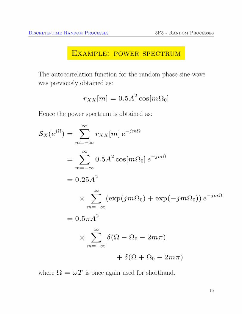
Discrete-time Random Processes 3F3 - Random Processes
Example power spectrum
The autocorrelation function for the random phase sine-wave
was previously obtained as
rXX[m] = 05A2cos[mΩ0]
Hence the power spectrum is obtained as
SX(ejΩ
) =
infinsumm=minusinfin
rXX[m] eminusjmΩ
=
infinsumm=minusinfin
05A2cos[mΩ0] e
minusjmΩ
= 025A2
timesinfinsum
m=minusinfin(exp(jmΩ0) + exp(minusjmΩ0)) e
minusjmΩ
= 05πA2
timesinfinsum
m=minusinfinδ(Ωminus Ω0 minus 2mπ)
+ δ(Ω + Ω0 minus 2mπ)
where Ω = ωT is once again used for shorthand
16
Discrete-time Random Processes 3F3 - Random Processes
Figure 3 Power spectrum of harmonic process
17
Discrete-time Random Processes 3F3 - Random Processes
White noise
White noise is defined in terms of its auto-covariance function
A wide sense stationary process is termed white noise if
cXX[m] = E[(Xn minus micro)(Xn+m minus micro)] = σ2Xδ[m]
where δ[m] is the discrete impulse function
δ[m] =
1 m = 0
0 otherwise
σ2X = E[(Xn minus micro)2] is the variance of the process If micro = 0
then σ2X is the mean-squared value of the process which we
will sometimes refer to as the lsquopowerrsquo
The power spectrum of zero mean white noise is
SX(ejωT
) =infinsum
m=minusinfinrXX[m] e
minusjmΩ
= σ2X
ie flat across all frequencies
18
Discrete-time Random Processes 3F3 - Random Processes
Example white Gaussian noise (WGN)
There are many ways to generate white noise processes all
having the property
cXX[m] = E[(Xn minus micro)(Xn+m minus micro)] = σ2Xδ[m]
The ensemble illustrated earlier in Fig was the zero-mean
Gaussian white noise process In this process the values Xn
are drawn independently from a Gaussian distribution with
mean 0 and variance σ2X
The N th order pdf for the Gaussian white noise process is
fXn1 Xn2 XnN(α1 α2 αN)
=Nprodi=1
N (αi|0 σ2X)
where
N (α|micro σ2) =
1radic
2πσ2exp
(minus
1
2σ2(xminus micro)
2
)is the univariate normal pdf
19
Discrete-time Random Processes 3F3 - Random Processes
We can immediately see that the Gaussian white noise process
is Strict sense stationary since
fXn1 Xn2 XnN(α1 α2 αN)
=Nprodi=1
N (αi|0 σ2X)
= fXn1+cXn2+c XnN+c (α1 α2 αN)
20
Discrete-time Random Processes 3F3 - Random Processes
21
Discrete-time Random Processes 3F3 - Random Processes
Linear systems and random processes
Figure 4 Linear system
When a wide-sense stationary discrete random process Xn is
passed through a stable linear time invariant (LTI) system with
22
Discrete-time Random Processes 3F3 - Random Processes
digital impulse response hn the output process Yn ie
yn =+infinsum
k=minusinfin
hk xnminusk = xn lowast hn
is also wide-sense stationary
23
Discrete-time Random Processes 3F3 - Random Processes
We can express the output correlation functions and power
spectra in terms of the input statistics and the LTI system
rXY [k] =E[Xn Yn+k] =
infinsuml=minusinfin
hl rXX[k minus l] = hk lowast rXX[k] (3)
Cross-correlation function at the output of a LTI system
rY Y [l] = E[Yn Yn+l]
infinsumk=minusinfin
infinsumi=minusinfin
hk hi rXX[l + iminus k] = hl lowast hminusl lowast rXX[l]
(4)
Autocorrelation function at the output of a LTI system
24
Discrete-time Random Processes 3F3 - Random Processes
Note these are convolutions as in the continuous-time case
This is easily remembered through the following figure
25
Discrete-time Random Processes 3F3 - Random Processes
Figure 5 Linear system - correlation functions
Taking DTFT of both sides of (4)
SY (ejωT
) = |H(ejωT
)|2SX(ejωT
) (5)
26
Discrete-time Random Processes 3F3 - Random Processes
Power spectrum at the output of a LTI system
27
Discrete-time Random Processes 3F3 - Random Processes
Example Filtering white noise
Suppose we filter a zero mean white noise process Xn with a first
order finite impulse response (FIR) filter
yn =1sum
m=0
bm xnminusm or Y (z) = (b0 + b1zminus1
)X(z)
with b0 = 1 b1 = 09 This an example of a moving average
(MA) process
The impulse response of this causal filter is
hn = b0 b1 0 0
The autocorrelation function of Yn is obtained as
rY Y [l] = E[Yn Yn+l] = hl lowast hminusl lowast rXX[l] (6)
This convolution can be performed directly However it is more
straightforward in the frequency domain
The frequency response of the filter is
H(ejΩ
) = b0 + b1eminusjΩ
28
Discrete-time Random Processes 3F3 - Random Processes
The power spectrum of Xn (white noise) is
SX(ejΩ
) = σ2X
Hence the power spectrum of Yn is
SY (ejΩ
) = |H(ejΩ
)|2SX(ejΩ
)
= |b0 + b1eminusjΩ|2σ2
X
= (b0b1e+jΩ
+ (b20 + b
21) + b0b1e
minusjΩ)σ
2X
as shown in the figure overleaf Comparing this expression with the
DTFT of rY Y [m]
SY (ejΩ
) =
infinsumm=minusinfin
rY Y [m] eminusjmΩ
we can identify non-zero terms in the summation only when m =
minus1 0+1 as follows
rY Y [minus1] = σ2Xb0b1 rY Y [0] = σ
2X(b
20 + b
21)
rY Y [1] = σ2Xb0b1
29
Discrete-time Random Processes 3F3 - Random Processes
Figure 6 Power spectrum of filtered white noise
30
Discrete-time Random Processes 3F3 - Random Processes
Ergodic Random processes
bull For an Ergodic random process we can estimate expectations
by performing time-averaging on a single sample function eg
micro = E[Xn] = limNrarrinfin
1
N
Nminus1sumn=0
xn (Mean ergodic)
rXX[k] = limNrarrinfin
1
N
Nminus1sumn=0
xnxn+k (Correlation ergodic) (7)
bull As in the continuous-time case these formulae allow us to make
the following estimates for lsquosufficientlyrsquo large N
micro = E[Xn] asymp1
N
Nminus1sumn=0
xn (Mean ergodic)
rXX[k] asymp1
N
Nminus1sumn=0
xnxn+k (Correlation ergodic) (8)
Note however that this is implemented with a simple computer
code loop in discrete-time unlike the continuous-time case
which requires an approximate integrator circuit
Under what conditions is a random process ergodic
31
Discrete-time Random Processes 3F3 - Random Processes
bull It is hard in general to determine whether a given process is
ergodic
bull A necessary and sufficient condition for mean ergodicity is given
by
limNrarrinfin
1
N
Nminus1sumk=0
cXX[k] = 0
where cXX is the autocovariance function
cXX[k] = E[(Xn minus micro)(Xn+k minus micro)]
and micro = E[Xn]
bull A simpler sufficient condition for mean ergodiciy is that
cXX[0] ltinfin and
limNrarrinfin
cXX[N ] = 0
bull Correlation ergodicity can be studied by extensions of the above
theorems We will not require the details here
bull Unless otherwise stated we will always assume that the signals
we encounter are both wide-sense stationary and ergodic
Although neither of these will always be true it will usually be
acceptable to assume so in practice
32
Discrete-time Random Processes 3F3 - Random Processes
Example
Consider the very simple lsquodc levelrsquo random process
Xn = A
where A is a random variable having the standard (ie mean zero
variance=1) Gaussian distribution
f(A) = N (A|0 1)
The mean of the random process is
E[Xn] =
int infinminusinfin
xn(a)f(a)da =
int infinminusinfin
af(a)da = 0
Now consider a random sample function measured from the random
process say
xt = a0
The mean value of this particular sample function is E[a0] = a0
Since in general a0 6= 0 the process is clearly not mean ergodic
33
Check this using the mean ergodic theorem The autocovariance
function is
cXX[k] = E[(Xn minus micro)(Xn+k minus micro)]
= E[XnXn+k] = E[A2] = 1
Now
limNrarrinfin
1
N
Nminus1sumk=0
cXX[k] = (1timesN)N = 1 6= 0
Hence the theorem confirms our finding that the process is not
ergodic in the mean
While this example highlights a possible pitfall in assuming
ergodicity most of the processes we deal with will however be
ergodic see examples paper for the random phase sine-wave and
the white noise processes
Comment Complex-valued processes
The above theory is easily extended to complex valued processes
Xn = XRen +jXIm
n in which case the autocorrelation function
is defined as
rXX[k] = E[XlowastnXn+k]
Revision Continuous time random processes
Figure 7 Ensemble representation of a random process
bull A random process is an ensemble of functions X(t) ω representingthe set of all possible waveforms that we might observe for that process
[NB ω is identical to the random variable α in the 3F1 notes]
ω is a random variable with its own probability distribution Pω whichdetermines randomly which waveform X(t ω) is observed ω may becontinuous- or discrete-valued
As before we will often omit ω and refer simply to random processX(t)
bull The mean of a random process is defined as micro(t) = E[X(t)] and theautocorrelation function as rXX [t1 t2] = E[X(t1)X(t2)] Theproperties of expectation allow us to calculate these in (at least) twoways
micro(t) = E[X(t1)]
=
intxx fX(t)(x) dx
=
intωX(t ω) fω(ω)dω
rXX(t1 t2) = E[X(t1)X(t2)]
=
intx1
intx2
x1x2 fX(t1)X(t2)(x1 x2) dx1dx2
=
intωX(t1 ω)X(t2 ω)fω(ω)dω
ie directly in terms of the density functions for X(t) or indirectly interms of the density function for ω
bull A wide-sense stationary (WSS) process X(t) is defined such that itsmean is a constant and rXX(t1 t2) depends only upon the differenceτ = t2 minus t1 ie
E[X(t)] = micro rXX(τ) = E[X(t)X(t+ τ)] (9)
[Wide-sense stationarity is also referred to as lsquoweak stationarityrsquo]
bull The Power Spectrum or Spectral Density of a WSS random process isdefined as the Fourier Transform of rXX(τ)
SX(ω) =
int infinminusinfin
rXX(τ) eminusjωτ
dτ (10)
bull For an Ergodic random process we can estimate expectations byperforming time-averaging on a single sample function eg
micro = E[X(t)] = limDrarrinfin
1
2D
int +D
minusDx(t)dt
rXX(τ) = limDrarrinfin
1
2D
int +D
minusDx(t)x(t+ τ)dt
Therefore for ergodic random processes we can make estimates forthese quantities by integrating over some suitably large (but finite) timeinterval 2D eg
E[X(t)] asymp1
2D
int +D
minusDx(t)dt
rXX(τ) asymp1
2D
int +D
minusDx(t)x(t+ τ)dt
where x(t) is a waveform measured at random from the process
Section 2 Optimal Filtering
Parts of this section and Section 3 are adapted from material kindly
supplied by Prof Peter Rayner
bull Optimal filtering is an area in which we design filters that are
optimally adapted to the statistical characteristics of a random
process As such the area can be seen as a combination of
standard filter design for deterministic signals with the random
process theory of the previous section
bull This remarkable area was pioneered in the 1940rsquos by Norbert
Wiener who designed methods for optimal estimation of a
signal measured in noise Specifically consider the system in the
figure below
Figure 8 The general Wiener filtering problem
bull A desired signal dn is observed in noise vn
xn = dn + vn
bull Wiener showed how to design a linear filter which would
optimally estimate dn given just the noisy observations xn and
some assumptions about the statistics of the random signal and
noise processes This class of filters the Wiener filter forms
the basis of many fundamental signal processing applications
bull Typical applications include
Noise reduction eg for speech and music signals
Prediction of future values of a signal eg in finance
Noise cancellation eg for aircraft cockpit noise
Deconvolution eg removal of room acoustics
(dereverberation) or echo cancellation in telephony
bull The Wiener filter is a very powerful tool However it is only the
optimal linear estimator for stationary signals The Kalman
filter offers an extension for non-stationary signals via state
space models In cases where a linear filter is still not good
enough non-linear filtering techniques can be adopted See 4th
year Signal Processing and Control modules for more advanced
topics in these areas
The Discrete-time Wiener Filter
In a minor abuse of notation and following standard conventions
we will refer to both random variables and their possible values in
lower-case symbols as this should cause no ambiguity for this section
of work
Figure 9 Wiener Filter
bull In the most general case we can filter the observed signal xnwith an Infinite impulse response (IIR) filter having a
non-causal impulse response hp
hp p = minusinfin minus1 0 1 2 infin (11)
bull We filter the observed noisy signal using the filter hp to
obtain an estimate dn of the desired signal
dn =infinsum
p=minusinfinhp xnminusp (12)
bull Since both dn and xn are drawn from random processes dnand xn we can only measure performance of the filter in
terms of expectations The criterion adopted for Wiener
filtering is the mean-squared error (MSE) criterion First
form the error signal εn
εn = dn minus dn = dn minusinfinsum
p=minusinfinhp xnminusp
The mean-squared error (MSE) is then defined as
J = E[ε2n] (13)
bull The Wiener filter minimises J with respect to the filter
coefficients hp
Derivation of Wiener filter
The Wiener filter assumes that xn and dn are jointly wide-
sense stationary This means that the means of both processes
are constant and all autocorrelation functionscross-correlation
functions (eg rxd[nm]) depend only on the time differencemminusnbetween data points
The expected error (13) may be minimised with respect to the
impulse response values hq A sufficient condition for a minimum
is
partJ
parthq=partE[ε2
n]
parthq= E
[partε2
n
parthq
]= E
[2εn
partεn
parthq
]= 0
for each q isin minusinfin minus1 0 1 2 infin
The term partεnparthq
is then calculated as
partεn
parthq=
part
parthq
dn minusinfinsum
p=minusinfinhp xnminusp
= minusxnminusq
and hence the coefficients must satisfy
E [εn xnminusq] = 0 minusinfin lt q lt +infin (14)
This is known as the orthogonality principle since two random
variables X and Y are termed orthogonal if
E[XY ] = 0
Now substituting for εn in (14) gives
E [εn xnminusq] = E
dn minus infinsump=minusinfin
hp xnminusp
xnminusq
= E [dn xnminusq]minus
infinsump=minusinfin
hp E [xnminusq xnminusp]
= rxd[q]minusinfinsum
p=minusinfinhp rxx[q minus p]
= 0
Hence rearranging the solution must satisfy
infinsump=minusinfin
hp rxx[q minus p] = rxd[q] minusinfin lt q lt +infin (15)
This is known as the Wiener-Hopf equations
The Wiener-Hopf equations involve an infinite number of unknowns
hq The simplest way to solve this is in the frequency domain First
note that the Wiener-Hopf equations can be rewritten as a discrete-
time convolution
hq lowast rxx[q] = rxd[q] minusinfin lt q lt +infin (16)
Taking discrete-time Fourier transforms (DTFT) of both sides
H(ejΩ
)Sx(ejΩ) = Sxd(ejΩ)
where Sxd(ejΩ) the DTFT of rxd[q] is defined as the cross-power
spectrum of d and x
Hence rearranging
H(ejΩ
) =Sxd(ejΩ)
Sx(ejΩ)(17)
Frequency domain Wiener filter
Mean-squared error for the optimal filter
The previous equations show how to calculate the optimal filter for
a given problem They donrsquot however tell us how well that optimal
filter performs This can be assessed from the mean-squared error
value of the optimal filter
J = E[ε2n] = E[εn(dn minus
infinsump=minusinfin
hp xnminusp)]
= E[εn dn]minusinfinsum
p=minusinfinhpE[εn xnminusp]
The expectation on the right is zero however for the optimal filter
by the orthogonality condition (14) so the minimum error is
Jmin = E[εn dn]
= E[(dn minusinfinsum
p=minusinfinhp xnminusp) dn]
= rdd[0]minusinfinsum
p=minusinfinhp rxd[p]
Important Special Case Uncorrelated Signal and Noise Processes
An important sub-class of the Wiener filter which also gives
considerable insight into filter behaviour can be gained by
considering the case where the desired signal process dn is
uncorrelated with the noise process vn ie
rdv[k] = E[dnvn+k] = 0 minusinfin lt k lt +infin
Consider the implications of this fact on the correlation functions
required in the Wiener-Hopf equations
infinsump=minusinfin
hp rxx[q minus p] = rxd[q] minusinfin lt q lt +infin
1 rxd
rxd[q] = E[xndn+q] = E[(dn + vn)dn+q] (18)
= E[dndn+q] + E[vndn+q] = rdd[q] (19)
since dn and vn are uncorrelated
Hence taking DTFT of both sides
Sxd(ejΩ) = Sd(ejΩ)
2 rxx
rxx[q] = E[xnxn+q] = E[(dn + vn)(dn+q + vn+q)]
= E[dndn+q] + E[vnvn+q] + E[dnvn+q] + E[vndn+q]
= E[dndn+q] + E[vnvn+q] = rdd[q] + rvv[q]
Hence
Sx(ejΩ) = Sd(ejΩ) + Sv(ejΩ)
Thus the Wiener filter becomes
H(ejΩ
) =Sd(ejΩ)
Sd(ejΩ) + Sv(ejΩ)
From this it can be seen that the behaviour of the filter is intuitively
reasonable in that at those frequencies where the noise power
spectrum Sv(ejΩ) is small the gain of the filter tends to unity
whereas the gain tends to a small value at those frequencies where the
noise spectrum is significantly larger than the desired signal power
spectrum Sd(ejΩ)
Example AR Process
An autoregressive process Dn of order 1 (see section 3) has power
spectrum
SD(ejΩ
) =σ2e
(1minus a1eminusjΩ)(1minus a1ejΩ)
Suppose the process is observed in zero mean white noise with
variance σ2v which is uncorrelated with Dn
xn = dn + vn
Design the Wiener filter for estimation of dn
Since the noise and desired signal are uncorrelated we can use the
form of Wiener filter from the previous page Substituting in the
various terms and rearranging its frequency response is
H(ejΩ
) =σ2e
σ2e + σ2
v(1minus a1eminusjΩ)(1minus a1ejΩ)
The impulse response of the filter can be found by inverse Fourier
transforming the frequency response This is studied in the examples
paper
The FIR Wiener filter
Note that in general the Wiener filter given by equation (17) is
non-causal and hence physically unrealisable in that the impulse
response hp is defined for values of p less than 0 Here we consider a
practical alternative in which a causal FIR Wiener filter is developed
In the FIR case the signal estimate is formed as
dn =
Pminus1sump=0
hp xnminusp (20)
and we minimise as before the objective function
J = E[(dn minus dn)2]
The filter derivation proceeds as before leading to an orthogonality
principle
E [εn xnminusq] = 0 q = 0 P minus 1 (21)
and Wiener-Hopf equations as follows
Pminus1sump=0
hp rxx[q minus p] = rxd[q] q = 0 1 P minus 1
(22)
The above equations may be written in matrix form as
Rxh = rxd
where
h =
h0
h1
hPminus1
rxd =
rxd[0]
rxd[1]
rxd[P minus 1]
and
Rx =
rxx[0] rxx[1] middot middot middot rxx[P minus 1]
rxx[1] rxx[0] rxx[P minus 2]
rxx[P minus 1] rxx[P minus 2] middot middot middot rxx[0]
Rx is known as the correlation matrix
Note that rxx[k] = rxx[minusk] so that the correlation matrix Rx
is symmetric and has constant diagonals (a symmetric Toeplitz
matrix)
The coefficient vector can be found by matrix inversion
h = Rxminus1
rxd (23)
This is the FIR Wiener filter and as for the general Wiener filter it
requires a-priori knowledge of the autocorrelation matrix Rx of the
input process xn and the cross-correlation rxd between the input
xn and the desired signal process dn
As before the minimum mean-squared error is given by
Jmin = E[εn dn]
= E[(dn minusPminus1sump=0
hp xnminusp) dn]
= rdd[0]minusPminus1sump=0
hp rxd[p]
= rdd[0]minus rTxdh = rdd[0]minus r
TxdRx
minus1rxd
Case Study Audio Noise Reduction
bull Consider a section of acoustic waveform (music voice ) dnthat is corrupted by additive noise vn
xn = dn + vn
bull We could try and noise reduce the signal using the FIR Wiener
filter
bull Assume that the section of data is wide-sense stationary and
ergodic (approx true for a short segment around 140 s)
Assume also that the noise is white and uncorrelated with the
audio signal - with variance σ2v ie
rvv[k] = σ2vδ[k]
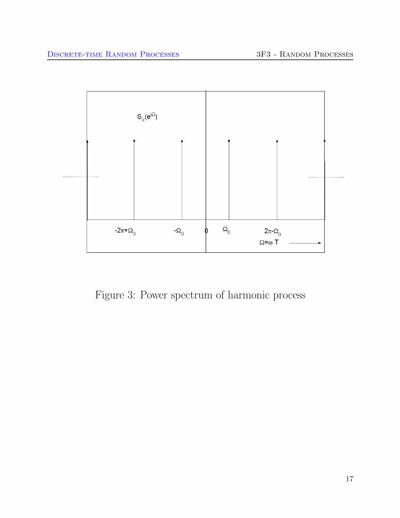
Discrete-time Random Processes 3F3 - Random Processes
Figure 3 Power spectrum of harmonic process
17
Discrete-time Random Processes 3F3 - Random Processes
White noise
White noise is defined in terms of its auto-covariance function
A wide sense stationary process is termed white noise if
cXX[m] = E[(Xn minus micro)(Xn+m minus micro)] = σ2Xδ[m]
where δ[m] is the discrete impulse function
δ[m] =
1 m = 0
0 otherwise
σ2X = E[(Xn minus micro)2] is the variance of the process If micro = 0
then σ2X is the mean-squared value of the process which we
will sometimes refer to as the lsquopowerrsquo
The power spectrum of zero mean white noise is
SX(ejωT
) =infinsum
m=minusinfinrXX[m] e
minusjmΩ
= σ2X
ie flat across all frequencies
18
Discrete-time Random Processes 3F3 - Random Processes
Example white Gaussian noise (WGN)
There are many ways to generate white noise processes all
having the property
cXX[m] = E[(Xn minus micro)(Xn+m minus micro)] = σ2Xδ[m]
The ensemble illustrated earlier in Fig was the zero-mean
Gaussian white noise process In this process the values Xn
are drawn independently from a Gaussian distribution with
mean 0 and variance σ2X
The N th order pdf for the Gaussian white noise process is
fXn1 Xn2 XnN(α1 α2 αN)
=Nprodi=1
N (αi|0 σ2X)
where
N (α|micro σ2) =
1radic
2πσ2exp
(minus
1
2σ2(xminus micro)
2
)is the univariate normal pdf
19
Discrete-time Random Processes 3F3 - Random Processes
We can immediately see that the Gaussian white noise process
is Strict sense stationary since
fXn1 Xn2 XnN(α1 α2 αN)
=Nprodi=1
N (αi|0 σ2X)
= fXn1+cXn2+c XnN+c (α1 α2 αN)
20
Discrete-time Random Processes 3F3 - Random Processes
21
Discrete-time Random Processes 3F3 - Random Processes
Linear systems and random processes
Figure 4 Linear system
When a wide-sense stationary discrete random process Xn is
passed through a stable linear time invariant (LTI) system with
22
Discrete-time Random Processes 3F3 - Random Processes
digital impulse response hn the output process Yn ie
yn =+infinsum
k=minusinfin
hk xnminusk = xn lowast hn
is also wide-sense stationary
23
Discrete-time Random Processes 3F3 - Random Processes
We can express the output correlation functions and power
spectra in terms of the input statistics and the LTI system
rXY [k] =E[Xn Yn+k] =
infinsuml=minusinfin
hl rXX[k minus l] = hk lowast rXX[k] (3)
Cross-correlation function at the output of a LTI system
rY Y [l] = E[Yn Yn+l]
infinsumk=minusinfin
infinsumi=minusinfin
hk hi rXX[l + iminus k] = hl lowast hminusl lowast rXX[l]
(4)
Autocorrelation function at the output of a LTI system
24
Discrete-time Random Processes 3F3 - Random Processes
Note these are convolutions as in the continuous-time case
This is easily remembered through the following figure
25
Discrete-time Random Processes 3F3 - Random Processes
Figure 5 Linear system - correlation functions
Taking DTFT of both sides of (4)
SY (ejωT
) = |H(ejωT
)|2SX(ejωT
) (5)
26
Discrete-time Random Processes 3F3 - Random Processes
Power spectrum at the output of a LTI system
27
Discrete-time Random Processes 3F3 - Random Processes
Example Filtering white noise
Suppose we filter a zero mean white noise process Xn with a first
order finite impulse response (FIR) filter
yn =1sum
m=0
bm xnminusm or Y (z) = (b0 + b1zminus1
)X(z)
with b0 = 1 b1 = 09 This an example of a moving average
(MA) process
The impulse response of this causal filter is
hn = b0 b1 0 0
The autocorrelation function of Yn is obtained as
rY Y [l] = E[Yn Yn+l] = hl lowast hminusl lowast rXX[l] (6)
This convolution can be performed directly However it is more
straightforward in the frequency domain
The frequency response of the filter is
H(ejΩ
) = b0 + b1eminusjΩ
28
Discrete-time Random Processes 3F3 - Random Processes
The power spectrum of Xn (white noise) is
SX(ejΩ
) = σ2X
Hence the power spectrum of Yn is
SY (ejΩ
) = |H(ejΩ
)|2SX(ejΩ
)
= |b0 + b1eminusjΩ|2σ2
X
= (b0b1e+jΩ
+ (b20 + b
21) + b0b1e
minusjΩ)σ
2X
as shown in the figure overleaf Comparing this expression with the
DTFT of rY Y [m]
SY (ejΩ
) =
infinsumm=minusinfin
rY Y [m] eminusjmΩ
we can identify non-zero terms in the summation only when m =
minus1 0+1 as follows
rY Y [minus1] = σ2Xb0b1 rY Y [0] = σ
2X(b
20 + b
21)
rY Y [1] = σ2Xb0b1
29
Discrete-time Random Processes 3F3 - Random Processes
Figure 6 Power spectrum of filtered white noise
30
Discrete-time Random Processes 3F3 - Random Processes
Ergodic Random processes
bull For an Ergodic random process we can estimate expectations
by performing time-averaging on a single sample function eg
micro = E[Xn] = limNrarrinfin
1
N
Nminus1sumn=0
xn (Mean ergodic)
rXX[k] = limNrarrinfin
1
N
Nminus1sumn=0
xnxn+k (Correlation ergodic) (7)
bull As in the continuous-time case these formulae allow us to make
the following estimates for lsquosufficientlyrsquo large N
micro = E[Xn] asymp1
N
Nminus1sumn=0
xn (Mean ergodic)
rXX[k] asymp1
N
Nminus1sumn=0
xnxn+k (Correlation ergodic) (8)
Note however that this is implemented with a simple computer
code loop in discrete-time unlike the continuous-time case
which requires an approximate integrator circuit
Under what conditions is a random process ergodic
31
Discrete-time Random Processes 3F3 - Random Processes
bull It is hard in general to determine whether a given process is
ergodic
bull A necessary and sufficient condition for mean ergodicity is given
by
limNrarrinfin
1
N
Nminus1sumk=0
cXX[k] = 0
where cXX is the autocovariance function
cXX[k] = E[(Xn minus micro)(Xn+k minus micro)]
and micro = E[Xn]
bull A simpler sufficient condition for mean ergodiciy is that
cXX[0] ltinfin and
limNrarrinfin
cXX[N ] = 0
bull Correlation ergodicity can be studied by extensions of the above
theorems We will not require the details here
bull Unless otherwise stated we will always assume that the signals
we encounter are both wide-sense stationary and ergodic
Although neither of these will always be true it will usually be
acceptable to assume so in practice
32
Discrete-time Random Processes 3F3 - Random Processes
Example
Consider the very simple lsquodc levelrsquo random process
Xn = A
where A is a random variable having the standard (ie mean zero
variance=1) Gaussian distribution
f(A) = N (A|0 1)
The mean of the random process is
E[Xn] =
int infinminusinfin
xn(a)f(a)da =
int infinminusinfin
af(a)da = 0
Now consider a random sample function measured from the random
process say
xt = a0
The mean value of this particular sample function is E[a0] = a0
Since in general a0 6= 0 the process is clearly not mean ergodic
33
Check this using the mean ergodic theorem The autocovariance
function is
cXX[k] = E[(Xn minus micro)(Xn+k minus micro)]
= E[XnXn+k] = E[A2] = 1
Now
limNrarrinfin
1
N
Nminus1sumk=0
cXX[k] = (1timesN)N = 1 6= 0
Hence the theorem confirms our finding that the process is not
ergodic in the mean
While this example highlights a possible pitfall in assuming
ergodicity most of the processes we deal with will however be
ergodic see examples paper for the random phase sine-wave and
the white noise processes
Comment Complex-valued processes
The above theory is easily extended to complex valued processes
Xn = XRen +jXIm
n in which case the autocorrelation function
is defined as
rXX[k] = E[XlowastnXn+k]
Revision Continuous time random processes
Figure 7 Ensemble representation of a random process
bull A random process is an ensemble of functions X(t) ω representingthe set of all possible waveforms that we might observe for that process
[NB ω is identical to the random variable α in the 3F1 notes]
ω is a random variable with its own probability distribution Pω whichdetermines randomly which waveform X(t ω) is observed ω may becontinuous- or discrete-valued
As before we will often omit ω and refer simply to random processX(t)
bull The mean of a random process is defined as micro(t) = E[X(t)] and theautocorrelation function as rXX [t1 t2] = E[X(t1)X(t2)] Theproperties of expectation allow us to calculate these in (at least) twoways
micro(t) = E[X(t1)]
=
intxx fX(t)(x) dx
=
intωX(t ω) fω(ω)dω
rXX(t1 t2) = E[X(t1)X(t2)]
=
intx1
intx2
x1x2 fX(t1)X(t2)(x1 x2) dx1dx2
=
intωX(t1 ω)X(t2 ω)fω(ω)dω
ie directly in terms of the density functions for X(t) or indirectly interms of the density function for ω
bull A wide-sense stationary (WSS) process X(t) is defined such that itsmean is a constant and rXX(t1 t2) depends only upon the differenceτ = t2 minus t1 ie
E[X(t)] = micro rXX(τ) = E[X(t)X(t+ τ)] (9)
[Wide-sense stationarity is also referred to as lsquoweak stationarityrsquo]
bull The Power Spectrum or Spectral Density of a WSS random process isdefined as the Fourier Transform of rXX(τ)
SX(ω) =
int infinminusinfin
rXX(τ) eminusjωτ
dτ (10)
bull For an Ergodic random process we can estimate expectations byperforming time-averaging on a single sample function eg
micro = E[X(t)] = limDrarrinfin
1
2D
int +D
minusDx(t)dt
rXX(τ) = limDrarrinfin
1
2D
int +D
minusDx(t)x(t+ τ)dt
Therefore for ergodic random processes we can make estimates forthese quantities by integrating over some suitably large (but finite) timeinterval 2D eg
E[X(t)] asymp1
2D
int +D
minusDx(t)dt
rXX(τ) asymp1
2D
int +D
minusDx(t)x(t+ τ)dt
where x(t) is a waveform measured at random from the process
Section 2 Optimal Filtering
Parts of this section and Section 3 are adapted from material kindly
supplied by Prof Peter Rayner
bull Optimal filtering is an area in which we design filters that are
optimally adapted to the statistical characteristics of a random
process As such the area can be seen as a combination of
standard filter design for deterministic signals with the random
process theory of the previous section
bull This remarkable area was pioneered in the 1940rsquos by Norbert
Wiener who designed methods for optimal estimation of a
signal measured in noise Specifically consider the system in the
figure below
Figure 8 The general Wiener filtering problem
bull A desired signal dn is observed in noise vn
xn = dn + vn
bull Wiener showed how to design a linear filter which would
optimally estimate dn given just the noisy observations xn and
some assumptions about the statistics of the random signal and
noise processes This class of filters the Wiener filter forms
the basis of many fundamental signal processing applications
bull Typical applications include
Noise reduction eg for speech and music signals
Prediction of future values of a signal eg in finance
Noise cancellation eg for aircraft cockpit noise
Deconvolution eg removal of room acoustics
(dereverberation) or echo cancellation in telephony
bull The Wiener filter is a very powerful tool However it is only the
optimal linear estimator for stationary signals The Kalman
filter offers an extension for non-stationary signals via state
space models In cases where a linear filter is still not good
enough non-linear filtering techniques can be adopted See 4th
year Signal Processing and Control modules for more advanced
topics in these areas
The Discrete-time Wiener Filter
In a minor abuse of notation and following standard conventions
we will refer to both random variables and their possible values in
lower-case symbols as this should cause no ambiguity for this section
of work
Figure 9 Wiener Filter
bull In the most general case we can filter the observed signal xnwith an Infinite impulse response (IIR) filter having a
non-causal impulse response hp
hp p = minusinfin minus1 0 1 2 infin (11)
bull We filter the observed noisy signal using the filter hp to
obtain an estimate dn of the desired signal
dn =infinsum
p=minusinfinhp xnminusp (12)
bull Since both dn and xn are drawn from random processes dnand xn we can only measure performance of the filter in
terms of expectations The criterion adopted for Wiener
filtering is the mean-squared error (MSE) criterion First
form the error signal εn
εn = dn minus dn = dn minusinfinsum
p=minusinfinhp xnminusp
The mean-squared error (MSE) is then defined as
J = E[ε2n] (13)
bull The Wiener filter minimises J with respect to the filter
coefficients hp
Derivation of Wiener filter
The Wiener filter assumes that xn and dn are jointly wide-
sense stationary This means that the means of both processes
are constant and all autocorrelation functionscross-correlation
functions (eg rxd[nm]) depend only on the time differencemminusnbetween data points
The expected error (13) may be minimised with respect to the
impulse response values hq A sufficient condition for a minimum
is
partJ
parthq=partE[ε2
n]
parthq= E
[partε2
n
parthq
]= E
[2εn
partεn
parthq
]= 0
for each q isin minusinfin minus1 0 1 2 infin
The term partεnparthq
is then calculated as
partεn
parthq=
part
parthq
dn minusinfinsum
p=minusinfinhp xnminusp
= minusxnminusq
and hence the coefficients must satisfy
E [εn xnminusq] = 0 minusinfin lt q lt +infin (14)
This is known as the orthogonality principle since two random
variables X and Y are termed orthogonal if
E[XY ] = 0
Now substituting for εn in (14) gives
E [εn xnminusq] = E
dn minus infinsump=minusinfin
hp xnminusp
xnminusq
= E [dn xnminusq]minus
infinsump=minusinfin
hp E [xnminusq xnminusp]
= rxd[q]minusinfinsum
p=minusinfinhp rxx[q minus p]
= 0
Hence rearranging the solution must satisfy
infinsump=minusinfin
hp rxx[q minus p] = rxd[q] minusinfin lt q lt +infin (15)
This is known as the Wiener-Hopf equations
The Wiener-Hopf equations involve an infinite number of unknowns
hq The simplest way to solve this is in the frequency domain First
note that the Wiener-Hopf equations can be rewritten as a discrete-
time convolution
hq lowast rxx[q] = rxd[q] minusinfin lt q lt +infin (16)
Taking discrete-time Fourier transforms (DTFT) of both sides
H(ejΩ
)Sx(ejΩ) = Sxd(ejΩ)
where Sxd(ejΩ) the DTFT of rxd[q] is defined as the cross-power
spectrum of d and x
Hence rearranging
H(ejΩ
) =Sxd(ejΩ)
Sx(ejΩ)(17)
Frequency domain Wiener filter
Mean-squared error for the optimal filter
The previous equations show how to calculate the optimal filter for
a given problem They donrsquot however tell us how well that optimal
filter performs This can be assessed from the mean-squared error
value of the optimal filter
J = E[ε2n] = E[εn(dn minus
infinsump=minusinfin
hp xnminusp)]
= E[εn dn]minusinfinsum
p=minusinfinhpE[εn xnminusp]
The expectation on the right is zero however for the optimal filter
by the orthogonality condition (14) so the minimum error is
Jmin = E[εn dn]
= E[(dn minusinfinsum
p=minusinfinhp xnminusp) dn]
= rdd[0]minusinfinsum
p=minusinfinhp rxd[p]
Important Special Case Uncorrelated Signal and Noise Processes
An important sub-class of the Wiener filter which also gives
considerable insight into filter behaviour can be gained by
considering the case where the desired signal process dn is
uncorrelated with the noise process vn ie
rdv[k] = E[dnvn+k] = 0 minusinfin lt k lt +infin
Consider the implications of this fact on the correlation functions
required in the Wiener-Hopf equations
infinsump=minusinfin
hp rxx[q minus p] = rxd[q] minusinfin lt q lt +infin
1 rxd
rxd[q] = E[xndn+q] = E[(dn + vn)dn+q] (18)
= E[dndn+q] + E[vndn+q] = rdd[q] (19)
since dn and vn are uncorrelated
Hence taking DTFT of both sides
Sxd(ejΩ) = Sd(ejΩ)
2 rxx
rxx[q] = E[xnxn+q] = E[(dn + vn)(dn+q + vn+q)]
= E[dndn+q] + E[vnvn+q] + E[dnvn+q] + E[vndn+q]
= E[dndn+q] + E[vnvn+q] = rdd[q] + rvv[q]
Hence
Sx(ejΩ) = Sd(ejΩ) + Sv(ejΩ)
Thus the Wiener filter becomes
H(ejΩ
) =Sd(ejΩ)
Sd(ejΩ) + Sv(ejΩ)
From this it can be seen that the behaviour of the filter is intuitively
reasonable in that at those frequencies where the noise power
spectrum Sv(ejΩ) is small the gain of the filter tends to unity
whereas the gain tends to a small value at those frequencies where the
noise spectrum is significantly larger than the desired signal power
spectrum Sd(ejΩ)
Example AR Process
An autoregressive process Dn of order 1 (see section 3) has power
spectrum
SD(ejΩ
) =σ2e
(1minus a1eminusjΩ)(1minus a1ejΩ)
Suppose the process is observed in zero mean white noise with
variance σ2v which is uncorrelated with Dn
xn = dn + vn
Design the Wiener filter for estimation of dn
Since the noise and desired signal are uncorrelated we can use the
form of Wiener filter from the previous page Substituting in the
various terms and rearranging its frequency response is
H(ejΩ
) =σ2e
σ2e + σ2
v(1minus a1eminusjΩ)(1minus a1ejΩ)
The impulse response of the filter can be found by inverse Fourier
transforming the frequency response This is studied in the examples
paper
The FIR Wiener filter
Note that in general the Wiener filter given by equation (17) is
non-causal and hence physically unrealisable in that the impulse
response hp is defined for values of p less than 0 Here we consider a
practical alternative in which a causal FIR Wiener filter is developed
In the FIR case the signal estimate is formed as
dn =
Pminus1sump=0
hp xnminusp (20)
and we minimise as before the objective function
J = E[(dn minus dn)2]
The filter derivation proceeds as before leading to an orthogonality
principle
E [εn xnminusq] = 0 q = 0 P minus 1 (21)
and Wiener-Hopf equations as follows
Pminus1sump=0
hp rxx[q minus p] = rxd[q] q = 0 1 P minus 1
(22)
The above equations may be written in matrix form as
Rxh = rxd
where
h =
h0
h1
hPminus1
rxd =
rxd[0]
rxd[1]
rxd[P minus 1]
and
Rx =
rxx[0] rxx[1] middot middot middot rxx[P minus 1]
rxx[1] rxx[0] rxx[P minus 2]
rxx[P minus 1] rxx[P minus 2] middot middot middot rxx[0]
Rx is known as the correlation matrix
Note that rxx[k] = rxx[minusk] so that the correlation matrix Rx
is symmetric and has constant diagonals (a symmetric Toeplitz
matrix)
The coefficient vector can be found by matrix inversion
h = Rxminus1
rxd (23)
This is the FIR Wiener filter and as for the general Wiener filter it
requires a-priori knowledge of the autocorrelation matrix Rx of the
input process xn and the cross-correlation rxd between the input
xn and the desired signal process dn
As before the minimum mean-squared error is given by
Jmin = E[εn dn]
= E[(dn minusPminus1sump=0
hp xnminusp) dn]
= rdd[0]minusPminus1sump=0
hp rxd[p]
= rdd[0]minus rTxdh = rdd[0]minus r
TxdRx
minus1rxd
Case Study Audio Noise Reduction
bull Consider a section of acoustic waveform (music voice ) dnthat is corrupted by additive noise vn
xn = dn + vn
bull We could try and noise reduce the signal using the FIR Wiener
filter
bull Assume that the section of data is wide-sense stationary and
ergodic (approx true for a short segment around 140 s)
Assume also that the noise is white and uncorrelated with the
audio signal - with variance σ2v ie
rvv[k] = σ2vδ[k]
Discrete-time Random Processes 3F3 - Random Processes
We can immediately see that the Gaussian white noise process
is Strict sense stationary since
fXn1 Xn2 XnN(α1 α2 αN)
=Nprodi=1
N (αi|0 σ2X)
= fXn1+cXn2+c XnN+c (α1 α2 αN)
20
Discrete-time Random Processes 3F3 - Random Processes
21
Discrete-time Random Processes 3F3 - Random Processes
Linear systems and random processes
Figure 4 Linear system
When a wide-sense stationary discrete random process Xn is
passed through a stable linear time invariant (LTI) system with
22
Discrete-time Random Processes 3F3 - Random Processes
digital impulse response hn the output process Yn ie
yn =+infinsum
k=minusinfin
hk xnminusk = xn lowast hn
is also wide-sense stationary
23
Discrete-time Random Processes 3F3 - Random Processes
We can express the output correlation functions and power
spectra in terms of the input statistics and the LTI system
rXY [k] =E[Xn Yn+k] =
infinsuml=minusinfin
hl rXX[k minus l] = hk lowast rXX[k] (3)
Cross-correlation function at the output of a LTI system
rY Y [l] = E[Yn Yn+l]
infinsumk=minusinfin
infinsumi=minusinfin
hk hi rXX[l + iminus k] = hl lowast hminusl lowast rXX[l]
(4)
Autocorrelation function at the output of a LTI system
24
Discrete-time Random Processes 3F3 - Random Processes
Note these are convolutions as in the continuous-time case
This is easily remembered through the following figure
25
Discrete-time Random Processes 3F3 - Random Processes
Figure 5 Linear system - correlation functions
Taking DTFT of both sides of (4)
SY (ejωT
) = |H(ejωT
)|2SX(ejωT
) (5)
26
Discrete-time Random Processes 3F3 - Random Processes
Power spectrum at the output of a LTI system
27
Discrete-time Random Processes 3F3 - Random Processes
Example Filtering white noise
Suppose we filter a zero mean white noise process Xn with a first
order finite impulse response (FIR) filter
yn =1sum
m=0
bm xnminusm or Y (z) = (b0 + b1zminus1
)X(z)
with b0 = 1 b1 = 09 This an example of a moving average
(MA) process
The impulse response of this causal filter is
hn = b0 b1 0 0
The autocorrelation function of Yn is obtained as
rY Y [l] = E[Yn Yn+l] = hl lowast hminusl lowast rXX[l] (6)
This convolution can be performed directly However it is more
straightforward in the frequency domain
The frequency response of the filter is
H(ejΩ
) = b0 + b1eminusjΩ
28
Discrete-time Random Processes 3F3 - Random Processes
The power spectrum of Xn (white noise) is
SX(ejΩ
) = σ2X
Hence the power spectrum of Yn is
SY (ejΩ
) = |H(ejΩ
)|2SX(ejΩ
)
= |b0 + b1eminusjΩ|2σ2
X
= (b0b1e+jΩ
+ (b20 + b
21) + b0b1e
minusjΩ)σ
2X
as shown in the figure overleaf Comparing this expression with the
DTFT of rY Y [m]
SY (ejΩ
) =
infinsumm=minusinfin
rY Y [m] eminusjmΩ
we can identify non-zero terms in the summation only when m =
minus1 0+1 as follows
rY Y [minus1] = σ2Xb0b1 rY Y [0] = σ
2X(b
20 + b
21)
rY Y [1] = σ2Xb0b1
29
Discrete-time Random Processes 3F3 - Random Processes
Figure 6 Power spectrum of filtered white noise
30
Discrete-time Random Processes 3F3 - Random Processes
Ergodic Random processes
bull For an Ergodic random process we can estimate expectations
by performing time-averaging on a single sample function eg
micro = E[Xn] = limNrarrinfin
1
N
Nminus1sumn=0
xn (Mean ergodic)
rXX[k] = limNrarrinfin
1
N
Nminus1sumn=0
xnxn+k (Correlation ergodic) (7)
bull As in the continuous-time case these formulae allow us to make
the following estimates for lsquosufficientlyrsquo large N
micro = E[Xn] asymp1
N
Nminus1sumn=0
xn (Mean ergodic)
rXX[k] asymp1
N
Nminus1sumn=0
xnxn+k (Correlation ergodic) (8)
Note however that this is implemented with a simple computer
code loop in discrete-time unlike the continuous-time case
which requires an approximate integrator circuit
Under what conditions is a random process ergodic
31
Discrete-time Random Processes 3F3 - Random Processes
bull It is hard in general to determine whether a given process is
ergodic
bull A necessary and sufficient condition for mean ergodicity is given
by
limNrarrinfin
1
N
Nminus1sumk=0
cXX[k] = 0
where cXX is the autocovariance function
cXX[k] = E[(Xn minus micro)(Xn+k minus micro)]
and micro = E[Xn]
bull A simpler sufficient condition for mean ergodiciy is that
cXX[0] ltinfin and
limNrarrinfin
cXX[N ] = 0
bull Correlation ergodicity can be studied by extensions of the above
theorems We will not require the details here
bull Unless otherwise stated we will always assume that the signals
we encounter are both wide-sense stationary and ergodic
Although neither of these will always be true it will usually be
acceptable to assume so in practice
32
Discrete-time Random Processes 3F3 - Random Processes
Example
Consider the very simple lsquodc levelrsquo random process
Xn = A
where A is a random variable having the standard (ie mean zero
variance=1) Gaussian distribution
f(A) = N (A|0 1)
The mean of the random process is
E[Xn] =
int infinminusinfin
xn(a)f(a)da =
int infinminusinfin
af(a)da = 0
Now consider a random sample function measured from the random
process say
xt = a0
The mean value of this particular sample function is E[a0] = a0
Since in general a0 6= 0 the process is clearly not mean ergodic
33
Check this using the mean ergodic theorem The autocovariance
function is
cXX[k] = E[(Xn minus micro)(Xn+k minus micro)]
= E[XnXn+k] = E[A2] = 1
Now
limNrarrinfin
1
N
Nminus1sumk=0
cXX[k] = (1timesN)N = 1 6= 0
Hence the theorem confirms our finding that the process is not
ergodic in the mean
While this example highlights a possible pitfall in assuming
ergodicity most of the processes we deal with will however be
ergodic see examples paper for the random phase sine-wave and
the white noise processes
Comment Complex-valued processes
The above theory is easily extended to complex valued processes
Xn = XRen +jXIm
n in which case the autocorrelation function
is defined as
rXX[k] = E[XlowastnXn+k]
Revision Continuous time random processes
Figure 7 Ensemble representation of a random process
bull A random process is an ensemble of functions X(t) ω representingthe set of all possible waveforms that we might observe for that process
[NB ω is identical to the random variable α in the 3F1 notes]
ω is a random variable with its own probability distribution Pω whichdetermines randomly which waveform X(t ω) is observed ω may becontinuous- or discrete-valued
As before we will often omit ω and refer simply to random processX(t)
bull The mean of a random process is defined as micro(t) = E[X(t)] and theautocorrelation function as rXX [t1 t2] = E[X(t1)X(t2)] Theproperties of expectation allow us to calculate these in (at least) twoways
micro(t) = E[X(t1)]
=
intxx fX(t)(x) dx
=
intωX(t ω) fω(ω)dω
rXX(t1 t2) = E[X(t1)X(t2)]
=
intx1
intx2
x1x2 fX(t1)X(t2)(x1 x2) dx1dx2
=
intωX(t1 ω)X(t2 ω)fω(ω)dω
ie directly in terms of the density functions for X(t) or indirectly interms of the density function for ω
bull A wide-sense stationary (WSS) process X(t) is defined such that itsmean is a constant and rXX(t1 t2) depends only upon the differenceτ = t2 minus t1 ie
E[X(t)] = micro rXX(τ) = E[X(t)X(t+ τ)] (9)
[Wide-sense stationarity is also referred to as lsquoweak stationarityrsquo]
bull The Power Spectrum or Spectral Density of a WSS random process isdefined as the Fourier Transform of rXX(τ)
SX(ω) =
int infinminusinfin
rXX(τ) eminusjωτ
dτ (10)
bull For an Ergodic random process we can estimate expectations byperforming time-averaging on a single sample function eg
micro = E[X(t)] = limDrarrinfin
1
2D
int +D
minusDx(t)dt
rXX(τ) = limDrarrinfin
1
2D
int +D
minusDx(t)x(t+ τ)dt
Therefore for ergodic random processes we can make estimates forthese quantities by integrating over some suitably large (but finite) timeinterval 2D eg
E[X(t)] asymp1
2D
int +D
minusDx(t)dt
rXX(τ) asymp1
2D
int +D
minusDx(t)x(t+ τ)dt
where x(t) is a waveform measured at random from the process
Section 2 Optimal Filtering
Parts of this section and Section 3 are adapted from material kindly
supplied by Prof Peter Rayner
bull Optimal filtering is an area in which we design filters that are
optimally adapted to the statistical characteristics of a random
process As such the area can be seen as a combination of
standard filter design for deterministic signals with the random
process theory of the previous section
bull This remarkable area was pioneered in the 1940rsquos by Norbert
Wiener who designed methods for optimal estimation of a
signal measured in noise Specifically consider the system in the
figure below
Figure 8 The general Wiener filtering problem
bull A desired signal dn is observed in noise vn
xn = dn + vn
bull Wiener showed how to design a linear filter which would
optimally estimate dn given just the noisy observations xn and
some assumptions about the statistics of the random signal and
noise processes This class of filters the Wiener filter forms
the basis of many fundamental signal processing applications
bull Typical applications include
Noise reduction eg for speech and music signals
Prediction of future values of a signal eg in finance
Noise cancellation eg for aircraft cockpit noise
Deconvolution eg removal of room acoustics
(dereverberation) or echo cancellation in telephony
bull The Wiener filter is a very powerful tool However it is only the
optimal linear estimator for stationary signals The Kalman
filter offers an extension for non-stationary signals via state
space models In cases where a linear filter is still not good
enough non-linear filtering techniques can be adopted See 4th
year Signal Processing and Control modules for more advanced
topics in these areas
The Discrete-time Wiener Filter
In a minor abuse of notation and following standard conventions
we will refer to both random variables and their possible values in
lower-case symbols as this should cause no ambiguity for this section
of work
Figure 9 Wiener Filter
bull In the most general case we can filter the observed signal xnwith an Infinite impulse response (IIR) filter having a
non-causal impulse response hp
hp p = minusinfin minus1 0 1 2 infin (11)
bull We filter the observed noisy signal using the filter hp to
obtain an estimate dn of the desired signal
dn =infinsum
p=minusinfinhp xnminusp (12)
bull Since both dn and xn are drawn from random processes dnand xn we can only measure performance of the filter in
terms of expectations The criterion adopted for Wiener
filtering is the mean-squared error (MSE) criterion First
form the error signal εn
εn = dn minus dn = dn minusinfinsum
p=minusinfinhp xnminusp
The mean-squared error (MSE) is then defined as
J = E[ε2n] (13)
bull The Wiener filter minimises J with respect to the filter
coefficients hp
Derivation of Wiener filter
The Wiener filter assumes that xn and dn are jointly wide-
sense stationary This means that the means of both processes
are constant and all autocorrelation functionscross-correlation
functions (eg rxd[nm]) depend only on the time differencemminusnbetween data points
The expected error (13) may be minimised with respect to the
impulse response values hq A sufficient condition for a minimum
is
partJ
parthq=partE[ε2
n]
parthq= E
[partε2
n
parthq
]= E
[2εn
partεn
parthq
]= 0
for each q isin minusinfin minus1 0 1 2 infin
The term partεnparthq
is then calculated as
partεn
parthq=
part
parthq
dn minusinfinsum
p=minusinfinhp xnminusp
= minusxnminusq
and hence the coefficients must satisfy
E [εn xnminusq] = 0 minusinfin lt q lt +infin (14)
This is known as the orthogonality principle since two random
variables X and Y are termed orthogonal if
E[XY ] = 0
Now substituting for εn in (14) gives
E [εn xnminusq] = E
dn minus infinsump=minusinfin
hp xnminusp
xnminusq
= E [dn xnminusq]minus
infinsump=minusinfin
hp E [xnminusq xnminusp]
= rxd[q]minusinfinsum
p=minusinfinhp rxx[q minus p]
= 0
Hence rearranging the solution must satisfy
infinsump=minusinfin
hp rxx[q minus p] = rxd[q] minusinfin lt q lt +infin (15)
This is known as the Wiener-Hopf equations
The Wiener-Hopf equations involve an infinite number of unknowns
hq The simplest way to solve this is in the frequency domain First
note that the Wiener-Hopf equations can be rewritten as a discrete-
time convolution
hq lowast rxx[q] = rxd[q] minusinfin lt q lt +infin (16)
Taking discrete-time Fourier transforms (DTFT) of both sides
H(ejΩ
)Sx(ejΩ) = Sxd(ejΩ)
where Sxd(ejΩ) the DTFT of rxd[q] is defined as the cross-power
spectrum of d and x
Hence rearranging
H(ejΩ
) =Sxd(ejΩ)
Sx(ejΩ)(17)
Frequency domain Wiener filter
Mean-squared error for the optimal filter
The previous equations show how to calculate the optimal filter for
a given problem They donrsquot however tell us how well that optimal
filter performs This can be assessed from the mean-squared error
value of the optimal filter
J = E[ε2n] = E[εn(dn minus
infinsump=minusinfin
hp xnminusp)]
= E[εn dn]minusinfinsum
p=minusinfinhpE[εn xnminusp]
The expectation on the right is zero however for the optimal filter
by the orthogonality condition (14) so the minimum error is
Jmin = E[εn dn]
= E[(dn minusinfinsum
p=minusinfinhp xnminusp) dn]
= rdd[0]minusinfinsum
p=minusinfinhp rxd[p]
Important Special Case Uncorrelated Signal and Noise Processes
An important sub-class of the Wiener filter which also gives
considerable insight into filter behaviour can be gained by
considering the case where the desired signal process dn is
uncorrelated with the noise process vn ie
rdv[k] = E[dnvn+k] = 0 minusinfin lt k lt +infin
Consider the implications of this fact on the correlation functions
required in the Wiener-Hopf equations
infinsump=minusinfin
hp rxx[q minus p] = rxd[q] minusinfin lt q lt +infin
1 rxd
rxd[q] = E[xndn+q] = E[(dn + vn)dn+q] (18)
= E[dndn+q] + E[vndn+q] = rdd[q] (19)
since dn and vn are uncorrelated
Hence taking DTFT of both sides
Sxd(ejΩ) = Sd(ejΩ)
2 rxx
rxx[q] = E[xnxn+q] = E[(dn + vn)(dn+q + vn+q)]
= E[dndn+q] + E[vnvn+q] + E[dnvn+q] + E[vndn+q]
= E[dndn+q] + E[vnvn+q] = rdd[q] + rvv[q]
Hence
Sx(ejΩ) = Sd(ejΩ) + Sv(ejΩ)
Thus the Wiener filter becomes
H(ejΩ
) =Sd(ejΩ)
Sd(ejΩ) + Sv(ejΩ)
From this it can be seen that the behaviour of the filter is intuitively
reasonable in that at those frequencies where the noise power
spectrum Sv(ejΩ) is small the gain of the filter tends to unity
whereas the gain tends to a small value at those frequencies where the
noise spectrum is significantly larger than the desired signal power
spectrum Sd(ejΩ)
Example AR Process
An autoregressive process Dn of order 1 (see section 3) has power
spectrum
SD(ejΩ
) =σ2e
(1minus a1eminusjΩ)(1minus a1ejΩ)
Suppose the process is observed in zero mean white noise with
variance σ2v which is uncorrelated with Dn
xn = dn + vn
Design the Wiener filter for estimation of dn
Since the noise and desired signal are uncorrelated we can use the
form of Wiener filter from the previous page Substituting in the
various terms and rearranging its frequency response is
H(ejΩ
) =σ2e
σ2e + σ2
v(1minus a1eminusjΩ)(1minus a1ejΩ)
The impulse response of the filter can be found by inverse Fourier
transforming the frequency response This is studied in the examples
paper
The FIR Wiener filter
Note that in general the Wiener filter given by equation (17) is
non-causal and hence physically unrealisable in that the impulse
response hp is defined for values of p less than 0 Here we consider a
practical alternative in which a causal FIR Wiener filter is developed
In the FIR case the signal estimate is formed as
dn =
Pminus1sump=0
hp xnminusp (20)
and we minimise as before the objective function
J = E[(dn minus dn)2]
The filter derivation proceeds as before leading to an orthogonality
principle
E [εn xnminusq] = 0 q = 0 P minus 1 (21)
and Wiener-Hopf equations as follows
Pminus1sump=0
hp rxx[q minus p] = rxd[q] q = 0 1 P minus 1
(22)
The above equations may be written in matrix form as
Rxh = rxd
where
h =
h0
h1
hPminus1
rxd =
rxd[0]
rxd[1]
rxd[P minus 1]
and
Rx =
rxx[0] rxx[1] middot middot middot rxx[P minus 1]
rxx[1] rxx[0] rxx[P minus 2]
rxx[P minus 1] rxx[P minus 2] middot middot middot rxx[0]
Rx is known as the correlation matrix
Note that rxx[k] = rxx[minusk] so that the correlation matrix Rx
is symmetric and has constant diagonals (a symmetric Toeplitz
matrix)
The coefficient vector can be found by matrix inversion
h = Rxminus1
rxd (23)
This is the FIR Wiener filter and as for the general Wiener filter it
requires a-priori knowledge of the autocorrelation matrix Rx of the
input process xn and the cross-correlation rxd between the input
xn and the desired signal process dn
As before the minimum mean-squared error is given by
Jmin = E[εn dn]
= E[(dn minusPminus1sump=0
hp xnminusp) dn]
= rdd[0]minusPminus1sump=0
hp rxd[p]
= rdd[0]minus rTxdh = rdd[0]minus r
TxdRx
minus1rxd
Case Study Audio Noise Reduction
bull Consider a section of acoustic waveform (music voice ) dnthat is corrupted by additive noise vn
xn = dn + vn
bull We could try and noise reduce the signal using the FIR Wiener
filter
bull Assume that the section of data is wide-sense stationary and
ergodic (approx true for a short segment around 140 s)
Assume also that the noise is white and uncorrelated with the
audio signal - with variance σ2v ie
rvv[k] = σ2vδ[k]

Discrete-time Random Processes 3F3 - Random Processes
21
Discrete-time Random Processes 3F3 - Random Processes
Linear systems and random processes
Figure 4 Linear system
When a wide-sense stationary discrete random process Xn is
passed through a stable linear time invariant (LTI) system with
22
Discrete-time Random Processes 3F3 - Random Processes
digital impulse response hn the output process Yn ie
yn =+infinsum
k=minusinfin
hk xnminusk = xn lowast hn
is also wide-sense stationary
23
Discrete-time Random Processes 3F3 - Random Processes
We can express the output correlation functions and power
spectra in terms of the input statistics and the LTI system
rXY [k] =E[Xn Yn+k] =
infinsuml=minusinfin
hl rXX[k minus l] = hk lowast rXX[k] (3)
Cross-correlation function at the output of a LTI system
rY Y [l] = E[Yn Yn+l]
infinsumk=minusinfin
infinsumi=minusinfin
hk hi rXX[l + iminus k] = hl lowast hminusl lowast rXX[l]
(4)
Autocorrelation function at the output of a LTI system
24
Discrete-time Random Processes 3F3 - Random Processes
Note these are convolutions as in the continuous-time case
This is easily remembered through the following figure
25
Discrete-time Random Processes 3F3 - Random Processes
Figure 5 Linear system - correlation functions
Taking DTFT of both sides of (4)
SY (ejωT
) = |H(ejωT
)|2SX(ejωT
) (5)
26
Discrete-time Random Processes 3F3 - Random Processes
Power spectrum at the output of a LTI system
27
Discrete-time Random Processes 3F3 - Random Processes
Example Filtering white noise
Suppose we filter a zero mean white noise process Xn with a first
order finite impulse response (FIR) filter
yn =1sum
m=0
bm xnminusm or Y (z) = (b0 + b1zminus1
)X(z)
with b0 = 1 b1 = 09 This an example of a moving average
(MA) process
The impulse response of this causal filter is
hn = b0 b1 0 0
The autocorrelation function of Yn is obtained as
rY Y [l] = E[Yn Yn+l] = hl lowast hminusl lowast rXX[l] (6)
This convolution can be performed directly However it is more
straightforward in the frequency domain
The frequency response of the filter is
H(ejΩ
) = b0 + b1eminusjΩ
28
Discrete-time Random Processes 3F3 - Random Processes
The power spectrum of Xn (white noise) is
SX(ejΩ
) = σ2X
Hence the power spectrum of Yn is
SY (ejΩ
) = |H(ejΩ
)|2SX(ejΩ
)
= |b0 + b1eminusjΩ|2σ2
X
= (b0b1e+jΩ
+ (b20 + b
21) + b0b1e
minusjΩ)σ
2X
as shown in the figure overleaf Comparing this expression with the
DTFT of rY Y [m]
SY (ejΩ
) =
infinsumm=minusinfin
rY Y [m] eminusjmΩ
we can identify non-zero terms in the summation only when m =
minus1 0+1 as follows
rY Y [minus1] = σ2Xb0b1 rY Y [0] = σ
2X(b
20 + b
21)
rY Y [1] = σ2Xb0b1
29
Discrete-time Random Processes 3F3 - Random Processes
Figure 6 Power spectrum of filtered white noise
30
Discrete-time Random Processes 3F3 - Random Processes
Ergodic Random processes
bull For an Ergodic random process we can estimate expectations
by performing time-averaging on a single sample function eg
micro = E[Xn] = limNrarrinfin
1
N
Nminus1sumn=0
xn (Mean ergodic)
rXX[k] = limNrarrinfin
1
N
Nminus1sumn=0
xnxn+k (Correlation ergodic) (7)
bull As in the continuous-time case these formulae allow us to make
the following estimates for lsquosufficientlyrsquo large N
micro = E[Xn] asymp1
N
Nminus1sumn=0
xn (Mean ergodic)
rXX[k] asymp1
N
Nminus1sumn=0
xnxn+k (Correlation ergodic) (8)
Note however that this is implemented with a simple computer
code loop in discrete-time unlike the continuous-time case
which requires an approximate integrator circuit
Under what conditions is a random process ergodic
31
Discrete-time Random Processes 3F3 - Random Processes
bull It is hard in general to determine whether a given process is
ergodic
bull A necessary and sufficient condition for mean ergodicity is given
by
limNrarrinfin
1
N
Nminus1sumk=0
cXX[k] = 0
where cXX is the autocovariance function
cXX[k] = E[(Xn minus micro)(Xn+k minus micro)]
and micro = E[Xn]
bull A simpler sufficient condition for mean ergodiciy is that
cXX[0] ltinfin and
limNrarrinfin
cXX[N ] = 0
bull Correlation ergodicity can be studied by extensions of the above
theorems We will not require the details here
bull Unless otherwise stated we will always assume that the signals
we encounter are both wide-sense stationary and ergodic
Although neither of these will always be true it will usually be
acceptable to assume so in practice
32
Discrete-time Random Processes 3F3 - Random Processes
Example
Consider the very simple lsquodc levelrsquo random process
Xn = A
where A is a random variable having the standard (ie mean zero
variance=1) Gaussian distribution
f(A) = N (A|0 1)
The mean of the random process is
E[Xn] =
int infinminusinfin
xn(a)f(a)da =
int infinminusinfin
af(a)da = 0
Now consider a random sample function measured from the random
process say
xt = a0
The mean value of this particular sample function is E[a0] = a0
Since in general a0 6= 0 the process is clearly not mean ergodic
33
Check this using the mean ergodic theorem The autocovariance
function is
cXX[k] = E[(Xn minus micro)(Xn+k minus micro)]
= E[XnXn+k] = E[A2] = 1
Now
limNrarrinfin
1
N
Nminus1sumk=0
cXX[k] = (1timesN)N = 1 6= 0
Hence the theorem confirms our finding that the process is not
ergodic in the mean
While this example highlights a possible pitfall in assuming
ergodicity most of the processes we deal with will however be
ergodic see examples paper for the random phase sine-wave and
the white noise processes
Comment Complex-valued processes
The above theory is easily extended to complex valued processes
Xn = XRen +jXIm
n in which case the autocorrelation function
is defined as
rXX[k] = E[XlowastnXn+k]
Revision Continuous time random processes
Figure 7 Ensemble representation of a random process
bull A random process is an ensemble of functions X(t) ω representingthe set of all possible waveforms that we might observe for that process
[NB ω is identical to the random variable α in the 3F1 notes]
ω is a random variable with its own probability distribution Pω whichdetermines randomly which waveform X(t ω) is observed ω may becontinuous- or discrete-valued
As before we will often omit ω and refer simply to random processX(t)
bull The mean of a random process is defined as micro(t) = E[X(t)] and theautocorrelation function as rXX [t1 t2] = E[X(t1)X(t2)] Theproperties of expectation allow us to calculate these in (at least) twoways
micro(t) = E[X(t1)]
=
intxx fX(t)(x) dx
=
intωX(t ω) fω(ω)dω
rXX(t1 t2) = E[X(t1)X(t2)]
=
intx1
intx2
x1x2 fX(t1)X(t2)(x1 x2) dx1dx2
=
intωX(t1 ω)X(t2 ω)fω(ω)dω
ie directly in terms of the density functions for X(t) or indirectly interms of the density function for ω
bull A wide-sense stationary (WSS) process X(t) is defined such that itsmean is a constant and rXX(t1 t2) depends only upon the differenceτ = t2 minus t1 ie
E[X(t)] = micro rXX(τ) = E[X(t)X(t+ τ)] (9)
[Wide-sense stationarity is also referred to as lsquoweak stationarityrsquo]
bull The Power Spectrum or Spectral Density of a WSS random process isdefined as the Fourier Transform of rXX(τ)
SX(ω) =
int infinminusinfin
rXX(τ) eminusjωτ
dτ (10)
bull For an Ergodic random process we can estimate expectations byperforming time-averaging on a single sample function eg
micro = E[X(t)] = limDrarrinfin
1
2D
int +D
minusDx(t)dt
rXX(τ) = limDrarrinfin
1
2D
int +D
minusDx(t)x(t+ τ)dt
Therefore for ergodic random processes we can make estimates forthese quantities by integrating over some suitably large (but finite) timeinterval 2D eg
E[X(t)] asymp1
2D
int +D
minusDx(t)dt
rXX(τ) asymp1
2D
int +D
minusDx(t)x(t+ τ)dt
where x(t) is a waveform measured at random from the process
Section 2 Optimal Filtering
Parts of this section and Section 3 are adapted from material kindly
supplied by Prof Peter Rayner
bull Optimal filtering is an area in which we design filters that are
optimally adapted to the statistical characteristics of a random
process As such the area can be seen as a combination of
standard filter design for deterministic signals with the random
process theory of the previous section
bull This remarkable area was pioneered in the 1940rsquos by Norbert
Wiener who designed methods for optimal estimation of a
signal measured in noise Specifically consider the system in the
figure below
Figure 8 The general Wiener filtering problem
bull A desired signal dn is observed in noise vn
xn = dn + vn
bull Wiener showed how to design a linear filter which would
optimally estimate dn given just the noisy observations xn and
some assumptions about the statistics of the random signal and
noise processes This class of filters the Wiener filter forms
the basis of many fundamental signal processing applications
bull Typical applications include
Noise reduction eg for speech and music signals
Prediction of future values of a signal eg in finance
Noise cancellation eg for aircraft cockpit noise
Deconvolution eg removal of room acoustics
(dereverberation) or echo cancellation in telephony
bull The Wiener filter is a very powerful tool However it is only the
optimal linear estimator for stationary signals The Kalman
filter offers an extension for non-stationary signals via state
space models In cases where a linear filter is still not good
enough non-linear filtering techniques can be adopted See 4th
year Signal Processing and Control modules for more advanced
topics in these areas
The Discrete-time Wiener Filter
In a minor abuse of notation and following standard conventions
we will refer to both random variables and their possible values in
lower-case symbols as this should cause no ambiguity for this section
of work
Figure 9 Wiener Filter
bull In the most general case we can filter the observed signal xnwith an Infinite impulse response (IIR) filter having a
non-causal impulse response hp
hp p = minusinfin minus1 0 1 2 infin (11)
bull We filter the observed noisy signal using the filter hp to
obtain an estimate dn of the desired signal
dn =infinsum
p=minusinfinhp xnminusp (12)
bull Since both dn and xn are drawn from random processes dnand xn we can only measure performance of the filter in
terms of expectations The criterion adopted for Wiener
filtering is the mean-squared error (MSE) criterion First
form the error signal εn
εn = dn minus dn = dn minusinfinsum
p=minusinfinhp xnminusp
The mean-squared error (MSE) is then defined as
J = E[ε2n] (13)
bull The Wiener filter minimises J with respect to the filter
coefficients hp
Derivation of Wiener filter
The Wiener filter assumes that xn and dn are jointly wide-
sense stationary This means that the means of both processes
are constant and all autocorrelation functionscross-correlation
functions (eg rxd[nm]) depend only on the time differencemminusnbetween data points
The expected error (13) may be minimised with respect to the
impulse response values hq A sufficient condition for a minimum
is
partJ
parthq=partE[ε2
n]
parthq= E
[partε2
n
parthq
]= E
[2εn
partεn
parthq
]= 0
for each q isin minusinfin minus1 0 1 2 infin
The term partεnparthq
is then calculated as
partεn
parthq=
part
parthq
dn minusinfinsum
p=minusinfinhp xnminusp
= minusxnminusq
and hence the coefficients must satisfy
E [εn xnminusq] = 0 minusinfin lt q lt +infin (14)
This is known as the orthogonality principle since two random
variables X and Y are termed orthogonal if
E[XY ] = 0
Now substituting for εn in (14) gives
E [εn xnminusq] = E
dn minus infinsump=minusinfin
hp xnminusp
xnminusq
= E [dn xnminusq]minus
infinsump=minusinfin
hp E [xnminusq xnminusp]
= rxd[q]minusinfinsum
p=minusinfinhp rxx[q minus p]
= 0
Hence rearranging the solution must satisfy
infinsump=minusinfin
hp rxx[q minus p] = rxd[q] minusinfin lt q lt +infin (15)
This is known as the Wiener-Hopf equations
The Wiener-Hopf equations involve an infinite number of unknowns
hq The simplest way to solve this is in the frequency domain First
note that the Wiener-Hopf equations can be rewritten as a discrete-
time convolution
hq lowast rxx[q] = rxd[q] minusinfin lt q lt +infin (16)
Taking discrete-time Fourier transforms (DTFT) of both sides
H(ejΩ
)Sx(ejΩ) = Sxd(ejΩ)
where Sxd(ejΩ) the DTFT of rxd[q] is defined as the cross-power
spectrum of d and x
Hence rearranging
H(ejΩ
) =Sxd(ejΩ)
Sx(ejΩ)(17)
Frequency domain Wiener filter
Mean-squared error for the optimal filter
The previous equations show how to calculate the optimal filter for
a given problem They donrsquot however tell us how well that optimal
filter performs This can be assessed from the mean-squared error
value of the optimal filter
J = E[ε2n] = E[εn(dn minus
infinsump=minusinfin
hp xnminusp)]
= E[εn dn]minusinfinsum
p=minusinfinhpE[εn xnminusp]
The expectation on the right is zero however for the optimal filter
by the orthogonality condition (14) so the minimum error is
Jmin = E[εn dn]
= E[(dn minusinfinsum
p=minusinfinhp xnminusp) dn]
= rdd[0]minusinfinsum
p=minusinfinhp rxd[p]
Important Special Case Uncorrelated Signal and Noise Processes
An important sub-class of the Wiener filter which also gives
considerable insight into filter behaviour can be gained by
considering the case where the desired signal process dn is
uncorrelated with the noise process vn ie
rdv[k] = E[dnvn+k] = 0 minusinfin lt k lt +infin
Consider the implications of this fact on the correlation functions
required in the Wiener-Hopf equations
infinsump=minusinfin
hp rxx[q minus p] = rxd[q] minusinfin lt q lt +infin
1 rxd
rxd[q] = E[xndn+q] = E[(dn + vn)dn+q] (18)
= E[dndn+q] + E[vndn+q] = rdd[q] (19)
since dn and vn are uncorrelated
Hence taking DTFT of both sides
Sxd(ejΩ) = Sd(ejΩ)
2 rxx
rxx[q] = E[xnxn+q] = E[(dn + vn)(dn+q + vn+q)]
= E[dndn+q] + E[vnvn+q] + E[dnvn+q] + E[vndn+q]
= E[dndn+q] + E[vnvn+q] = rdd[q] + rvv[q]
Hence
Sx(ejΩ) = Sd(ejΩ) + Sv(ejΩ)
Thus the Wiener filter becomes
H(ejΩ
) =Sd(ejΩ)
Sd(ejΩ) + Sv(ejΩ)
From this it can be seen that the behaviour of the filter is intuitively
reasonable in that at those frequencies where the noise power
spectrum Sv(ejΩ) is small the gain of the filter tends to unity
whereas the gain tends to a small value at those frequencies where the
noise spectrum is significantly larger than the desired signal power
spectrum Sd(ejΩ)
Example AR Process
An autoregressive process Dn of order 1 (see section 3) has power
spectrum
SD(ejΩ
) =σ2e
(1minus a1eminusjΩ)(1minus a1ejΩ)
Suppose the process is observed in zero mean white noise with
variance σ2v which is uncorrelated with Dn
xn = dn + vn
Design the Wiener filter for estimation of dn
Since the noise and desired signal are uncorrelated we can use the
form of Wiener filter from the previous page Substituting in the
various terms and rearranging its frequency response is
H(ejΩ
) =σ2e
σ2e + σ2
v(1minus a1eminusjΩ)(1minus a1ejΩ)
The impulse response of the filter can be found by inverse Fourier
transforming the frequency response This is studied in the examples
paper
The FIR Wiener filter
Note that in general the Wiener filter given by equation (17) is
non-causal and hence physically unrealisable in that the impulse
response hp is defined for values of p less than 0 Here we consider a
practical alternative in which a causal FIR Wiener filter is developed
In the FIR case the signal estimate is formed as
dn =
Pminus1sump=0
hp xnminusp (20)
and we minimise as before the objective function
J = E[(dn minus dn)2]
The filter derivation proceeds as before leading to an orthogonality
principle
E [εn xnminusq] = 0 q = 0 P minus 1 (21)
and Wiener-Hopf equations as follows
Pminus1sump=0
hp rxx[q minus p] = rxd[q] q = 0 1 P minus 1
(22)
The above equations may be written in matrix form as
Rxh = rxd
where
h =
h0
h1
hPminus1
rxd =
rxd[0]
rxd[1]
rxd[P minus 1]
and
Rx =
rxx[0] rxx[1] middot middot middot rxx[P minus 1]
rxx[1] rxx[0] rxx[P minus 2]
rxx[P minus 1] rxx[P minus 2] middot middot middot rxx[0]
Rx is known as the correlation matrix
Note that rxx[k] = rxx[minusk] so that the correlation matrix Rx
is symmetric and has constant diagonals (a symmetric Toeplitz
matrix)
The coefficient vector can be found by matrix inversion
h = Rxminus1
rxd (23)
This is the FIR Wiener filter and as for the general Wiener filter it
requires a-priori knowledge of the autocorrelation matrix Rx of the
input process xn and the cross-correlation rxd between the input
xn and the desired signal process dn
As before the minimum mean-squared error is given by
Jmin = E[εn dn]
= E[(dn minusPminus1sump=0
hp xnminusp) dn]
= rdd[0]minusPminus1sump=0
hp rxd[p]
= rdd[0]minus rTxdh = rdd[0]minus r
TxdRx
minus1rxd
Case Study Audio Noise Reduction
bull Consider a section of acoustic waveform (music voice ) dnthat is corrupted by additive noise vn
xn = dn + vn
bull We could try and noise reduce the signal using the FIR Wiener
filter
bull Assume that the section of data is wide-sense stationary and
ergodic (approx true for a short segment around 140 s)
Assume also that the noise is white and uncorrelated with the
audio signal - with variance σ2v ie
rvv[k] = σ2vδ[k]
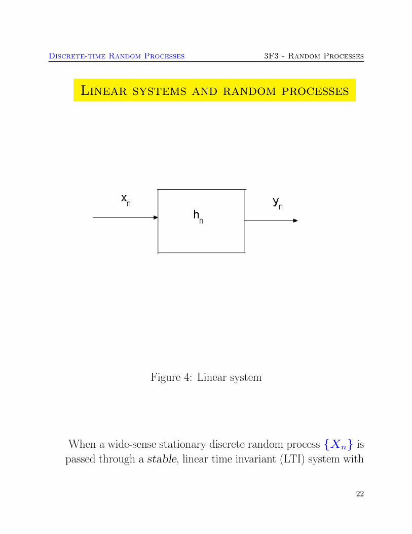
Discrete-time Random Processes 3F3 - Random Processes
Linear systems and random processes
Figure 4 Linear system
When a wide-sense stationary discrete random process Xn is
passed through a stable linear time invariant (LTI) system with
22
Discrete-time Random Processes 3F3 - Random Processes
digital impulse response hn the output process Yn ie
yn =+infinsum
k=minusinfin
hk xnminusk = xn lowast hn
is also wide-sense stationary
23
Discrete-time Random Processes 3F3 - Random Processes
We can express the output correlation functions and power
spectra in terms of the input statistics and the LTI system
rXY [k] =E[Xn Yn+k] =
infinsuml=minusinfin
hl rXX[k minus l] = hk lowast rXX[k] (3)
Cross-correlation function at the output of a LTI system
rY Y [l] = E[Yn Yn+l]
infinsumk=minusinfin
infinsumi=minusinfin
hk hi rXX[l + iminus k] = hl lowast hminusl lowast rXX[l]
(4)
Autocorrelation function at the output of a LTI system
24
Discrete-time Random Processes 3F3 - Random Processes
Note these are convolutions as in the continuous-time case
This is easily remembered through the following figure
25
Discrete-time Random Processes 3F3 - Random Processes
Figure 5 Linear system - correlation functions
Taking DTFT of both sides of (4)
SY (ejωT
) = |H(ejωT
)|2SX(ejωT
) (5)
26
Discrete-time Random Processes 3F3 - Random Processes
Power spectrum at the output of a LTI system
27
Discrete-time Random Processes 3F3 - Random Processes
Example Filtering white noise
Suppose we filter a zero mean white noise process Xn with a first
order finite impulse response (FIR) filter
yn =1sum
m=0
bm xnminusm or Y (z) = (b0 + b1zminus1
)X(z)
with b0 = 1 b1 = 09 This an example of a moving average
(MA) process
The impulse response of this causal filter is
hn = b0 b1 0 0
The autocorrelation function of Yn is obtained as
rY Y [l] = E[Yn Yn+l] = hl lowast hminusl lowast rXX[l] (6)
This convolution can be performed directly However it is more
straightforward in the frequency domain
The frequency response of the filter is
H(ejΩ
) = b0 + b1eminusjΩ
28
Discrete-time Random Processes 3F3 - Random Processes
The power spectrum of Xn (white noise) is
SX(ejΩ
) = σ2X
Hence the power spectrum of Yn is
SY (ejΩ
) = |H(ejΩ
)|2SX(ejΩ
)
= |b0 + b1eminusjΩ|2σ2
X
= (b0b1e+jΩ
+ (b20 + b
21) + b0b1e
minusjΩ)σ
2X
as shown in the figure overleaf Comparing this expression with the
DTFT of rY Y [m]
SY (ejΩ
) =
infinsumm=minusinfin
rY Y [m] eminusjmΩ
we can identify non-zero terms in the summation only when m =
minus1 0+1 as follows
rY Y [minus1] = σ2Xb0b1 rY Y [0] = σ
2X(b
20 + b
21)
rY Y [1] = σ2Xb0b1
29
Discrete-time Random Processes 3F3 - Random Processes
Figure 6 Power spectrum of filtered white noise
30
Discrete-time Random Processes 3F3 - Random Processes
Ergodic Random processes
bull For an Ergodic random process we can estimate expectations
by performing time-averaging on a single sample function eg
micro = E[Xn] = limNrarrinfin
1
N
Nminus1sumn=0
xn (Mean ergodic)
rXX[k] = limNrarrinfin
1
N
Nminus1sumn=0
xnxn+k (Correlation ergodic) (7)
bull As in the continuous-time case these formulae allow us to make
the following estimates for lsquosufficientlyrsquo large N
micro = E[Xn] asymp1
N
Nminus1sumn=0
xn (Mean ergodic)
rXX[k] asymp1
N
Nminus1sumn=0
xnxn+k (Correlation ergodic) (8)
Note however that this is implemented with a simple computer
code loop in discrete-time unlike the continuous-time case
which requires an approximate integrator circuit
Under what conditions is a random process ergodic
31
Discrete-time Random Processes 3F3 - Random Processes
bull It is hard in general to determine whether a given process is
ergodic
bull A necessary and sufficient condition for mean ergodicity is given
by
limNrarrinfin
1
N
Nminus1sumk=0
cXX[k] = 0
where cXX is the autocovariance function
cXX[k] = E[(Xn minus micro)(Xn+k minus micro)]
and micro = E[Xn]
bull A simpler sufficient condition for mean ergodiciy is that
cXX[0] ltinfin and
limNrarrinfin
cXX[N ] = 0
bull Correlation ergodicity can be studied by extensions of the above
theorems We will not require the details here
bull Unless otherwise stated we will always assume that the signals
we encounter are both wide-sense stationary and ergodic
Although neither of these will always be true it will usually be
acceptable to assume so in practice
32
Discrete-time Random Processes 3F3 - Random Processes
Example
Consider the very simple lsquodc levelrsquo random process
Xn = A
where A is a random variable having the standard (ie mean zero
variance=1) Gaussian distribution
f(A) = N (A|0 1)
The mean of the random process is
E[Xn] =
int infinminusinfin
xn(a)f(a)da =
int infinminusinfin
af(a)da = 0
Now consider a random sample function measured from the random
process say
xt = a0
The mean value of this particular sample function is E[a0] = a0
Since in general a0 6= 0 the process is clearly not mean ergodic
33
Check this using the mean ergodic theorem The autocovariance
function is
cXX[k] = E[(Xn minus micro)(Xn+k minus micro)]
= E[XnXn+k] = E[A2] = 1
Now
limNrarrinfin
1
N
Nminus1sumk=0
cXX[k] = (1timesN)N = 1 6= 0
Hence the theorem confirms our finding that the process is not
ergodic in the mean
While this example highlights a possible pitfall in assuming
ergodicity most of the processes we deal with will however be
ergodic see examples paper for the random phase sine-wave and
the white noise processes
Comment Complex-valued processes
The above theory is easily extended to complex valued processes
Xn = XRen +jXIm
n in which case the autocorrelation function
is defined as
rXX[k] = E[XlowastnXn+k]
Revision Continuous time random processes
Figure 7 Ensemble representation of a random process
bull A random process is an ensemble of functions X(t) ω representingthe set of all possible waveforms that we might observe for that process
[NB ω is identical to the random variable α in the 3F1 notes]
ω is a random variable with its own probability distribution Pω whichdetermines randomly which waveform X(t ω) is observed ω may becontinuous- or discrete-valued
As before we will often omit ω and refer simply to random processX(t)
bull The mean of a random process is defined as micro(t) = E[X(t)] and theautocorrelation function as rXX [t1 t2] = E[X(t1)X(t2)] Theproperties of expectation allow us to calculate these in (at least) twoways
micro(t) = E[X(t1)]
=
intxx fX(t)(x) dx
=
intωX(t ω) fω(ω)dω
rXX(t1 t2) = E[X(t1)X(t2)]
=
intx1
intx2
x1x2 fX(t1)X(t2)(x1 x2) dx1dx2
=
intωX(t1 ω)X(t2 ω)fω(ω)dω
ie directly in terms of the density functions for X(t) or indirectly interms of the density function for ω
bull A wide-sense stationary (WSS) process X(t) is defined such that itsmean is a constant and rXX(t1 t2) depends only upon the differenceτ = t2 minus t1 ie
E[X(t)] = micro rXX(τ) = E[X(t)X(t+ τ)] (9)
[Wide-sense stationarity is also referred to as lsquoweak stationarityrsquo]
bull The Power Spectrum or Spectral Density of a WSS random process isdefined as the Fourier Transform of rXX(τ)
SX(ω) =
int infinminusinfin
rXX(τ) eminusjωτ
dτ (10)
bull For an Ergodic random process we can estimate expectations byperforming time-averaging on a single sample function eg
micro = E[X(t)] = limDrarrinfin
1
2D
int +D
minusDx(t)dt
rXX(τ) = limDrarrinfin
1
2D
int +D
minusDx(t)x(t+ τ)dt
Therefore for ergodic random processes we can make estimates forthese quantities by integrating over some suitably large (but finite) timeinterval 2D eg
E[X(t)] asymp1
2D
int +D
minusDx(t)dt
rXX(τ) asymp1
2D
int +D
minusDx(t)x(t+ τ)dt
where x(t) is a waveform measured at random from the process
Section 2 Optimal Filtering
Parts of this section and Section 3 are adapted from material kindly
supplied by Prof Peter Rayner
bull Optimal filtering is an area in which we design filters that are
optimally adapted to the statistical characteristics of a random
process As such the area can be seen as a combination of
standard filter design for deterministic signals with the random
process theory of the previous section
bull This remarkable area was pioneered in the 1940rsquos by Norbert
Wiener who designed methods for optimal estimation of a
signal measured in noise Specifically consider the system in the
figure below
Figure 8 The general Wiener filtering problem
bull A desired signal dn is observed in noise vn
xn = dn + vn
bull Wiener showed how to design a linear filter which would
optimally estimate dn given just the noisy observations xn and
some assumptions about the statistics of the random signal and
noise processes This class of filters the Wiener filter forms
the basis of many fundamental signal processing applications
bull Typical applications include
Noise reduction eg for speech and music signals
Prediction of future values of a signal eg in finance
Noise cancellation eg for aircraft cockpit noise
Deconvolution eg removal of room acoustics
(dereverberation) or echo cancellation in telephony
bull The Wiener filter is a very powerful tool However it is only the
optimal linear estimator for stationary signals The Kalman
filter offers an extension for non-stationary signals via state
space models In cases where a linear filter is still not good
enough non-linear filtering techniques can be adopted See 4th
year Signal Processing and Control modules for more advanced
topics in these areas
The Discrete-time Wiener Filter
In a minor abuse of notation and following standard conventions
we will refer to both random variables and their possible values in
lower-case symbols as this should cause no ambiguity for this section
of work
Figure 9 Wiener Filter
bull In the most general case we can filter the observed signal xnwith an Infinite impulse response (IIR) filter having a
non-causal impulse response hp
hp p = minusinfin minus1 0 1 2 infin (11)
bull We filter the observed noisy signal using the filter hp to
obtain an estimate dn of the desired signal
dn =infinsum
p=minusinfinhp xnminusp (12)
bull Since both dn and xn are drawn from random processes dnand xn we can only measure performance of the filter in
terms of expectations The criterion adopted for Wiener
filtering is the mean-squared error (MSE) criterion First
form the error signal εn
εn = dn minus dn = dn minusinfinsum
p=minusinfinhp xnminusp
The mean-squared error (MSE) is then defined as
J = E[ε2n] (13)
bull The Wiener filter minimises J with respect to the filter
coefficients hp
Derivation of Wiener filter
The Wiener filter assumes that xn and dn are jointly wide-
sense stationary This means that the means of both processes
are constant and all autocorrelation functionscross-correlation
functions (eg rxd[nm]) depend only on the time differencemminusnbetween data points
The expected error (13) may be minimised with respect to the
impulse response values hq A sufficient condition for a minimum
is
partJ
parthq=partE[ε2
n]
parthq= E
[partε2
n
parthq
]= E
[2εn
partεn
parthq
]= 0
for each q isin minusinfin minus1 0 1 2 infin
The term partεnparthq
is then calculated as
partεn
parthq=
part
parthq
dn minusinfinsum
p=minusinfinhp xnminusp
= minusxnminusq
and hence the coefficients must satisfy
E [εn xnminusq] = 0 minusinfin lt q lt +infin (14)
This is known as the orthogonality principle since two random
variables X and Y are termed orthogonal if
E[XY ] = 0
Now substituting for εn in (14) gives
E [εn xnminusq] = E
dn minus infinsump=minusinfin
hp xnminusp
xnminusq
= E [dn xnminusq]minus
infinsump=minusinfin
hp E [xnminusq xnminusp]
= rxd[q]minusinfinsum
p=minusinfinhp rxx[q minus p]
= 0
Hence rearranging the solution must satisfy
infinsump=minusinfin
hp rxx[q minus p] = rxd[q] minusinfin lt q lt +infin (15)
This is known as the Wiener-Hopf equations
The Wiener-Hopf equations involve an infinite number of unknowns
hq The simplest way to solve this is in the frequency domain First
note that the Wiener-Hopf equations can be rewritten as a discrete-
time convolution
hq lowast rxx[q] = rxd[q] minusinfin lt q lt +infin (16)
Taking discrete-time Fourier transforms (DTFT) of both sides
H(ejΩ
)Sx(ejΩ) = Sxd(ejΩ)
where Sxd(ejΩ) the DTFT of rxd[q] is defined as the cross-power
spectrum of d and x
Hence rearranging
H(ejΩ
) =Sxd(ejΩ)
Sx(ejΩ)(17)
Frequency domain Wiener filter
Mean-squared error for the optimal filter
The previous equations show how to calculate the optimal filter for
a given problem They donrsquot however tell us how well that optimal
filter performs This can be assessed from the mean-squared error
value of the optimal filter
J = E[ε2n] = E[εn(dn minus
infinsump=minusinfin
hp xnminusp)]
= E[εn dn]minusinfinsum
p=minusinfinhpE[εn xnminusp]
The expectation on the right is zero however for the optimal filter
by the orthogonality condition (14) so the minimum error is
Jmin = E[εn dn]
= E[(dn minusinfinsum
p=minusinfinhp xnminusp) dn]
= rdd[0]minusinfinsum
p=minusinfinhp rxd[p]
Important Special Case Uncorrelated Signal and Noise Processes
An important sub-class of the Wiener filter which also gives
considerable insight into filter behaviour can be gained by
considering the case where the desired signal process dn is
uncorrelated with the noise process vn ie
rdv[k] = E[dnvn+k] = 0 minusinfin lt k lt +infin
Consider the implications of this fact on the correlation functions
required in the Wiener-Hopf equations
infinsump=minusinfin
hp rxx[q minus p] = rxd[q] minusinfin lt q lt +infin
1 rxd
rxd[q] = E[xndn+q] = E[(dn + vn)dn+q] (18)
= E[dndn+q] + E[vndn+q] = rdd[q] (19)
since dn and vn are uncorrelated
Hence taking DTFT of both sides
Sxd(ejΩ) = Sd(ejΩ)
2 rxx
rxx[q] = E[xnxn+q] = E[(dn + vn)(dn+q + vn+q)]
= E[dndn+q] + E[vnvn+q] + E[dnvn+q] + E[vndn+q]
= E[dndn+q] + E[vnvn+q] = rdd[q] + rvv[q]
Hence
Sx(ejΩ) = Sd(ejΩ) + Sv(ejΩ)
Thus the Wiener filter becomes
H(ejΩ
) =Sd(ejΩ)
Sd(ejΩ) + Sv(ejΩ)
From this it can be seen that the behaviour of the filter is intuitively
reasonable in that at those frequencies where the noise power
spectrum Sv(ejΩ) is small the gain of the filter tends to unity
whereas the gain tends to a small value at those frequencies where the
noise spectrum is significantly larger than the desired signal power
spectrum Sd(ejΩ)
Example AR Process
An autoregressive process Dn of order 1 (see section 3) has power
spectrum
SD(ejΩ
) =σ2e
(1minus a1eminusjΩ)(1minus a1ejΩ)
Suppose the process is observed in zero mean white noise with
variance σ2v which is uncorrelated with Dn
xn = dn + vn
Design the Wiener filter for estimation of dn
Since the noise and desired signal are uncorrelated we can use the
form of Wiener filter from the previous page Substituting in the
various terms and rearranging its frequency response is
H(ejΩ
) =σ2e
σ2e + σ2
v(1minus a1eminusjΩ)(1minus a1ejΩ)
The impulse response of the filter can be found by inverse Fourier
transforming the frequency response This is studied in the examples
paper
The FIR Wiener filter
Note that in general the Wiener filter given by equation (17) is
non-causal and hence physically unrealisable in that the impulse
response hp is defined for values of p less than 0 Here we consider a
practical alternative in which a causal FIR Wiener filter is developed
In the FIR case the signal estimate is formed as
dn =
Pminus1sump=0
hp xnminusp (20)
and we minimise as before the objective function
J = E[(dn minus dn)2]
The filter derivation proceeds as before leading to an orthogonality
principle
E [εn xnminusq] = 0 q = 0 P minus 1 (21)
and Wiener-Hopf equations as follows
Pminus1sump=0
hp rxx[q minus p] = rxd[q] q = 0 1 P minus 1
(22)
The above equations may be written in matrix form as
Rxh = rxd
where
h =
h0
h1
hPminus1
rxd =
rxd[0]
rxd[1]
rxd[P minus 1]
and
Rx =
rxx[0] rxx[1] middot middot middot rxx[P minus 1]
rxx[1] rxx[0] rxx[P minus 2]
rxx[P minus 1] rxx[P minus 2] middot middot middot rxx[0]
Rx is known as the correlation matrix
Note that rxx[k] = rxx[minusk] so that the correlation matrix Rx
is symmetric and has constant diagonals (a symmetric Toeplitz
matrix)
The coefficient vector can be found by matrix inversion
h = Rxminus1
rxd (23)
This is the FIR Wiener filter and as for the general Wiener filter it
requires a-priori knowledge of the autocorrelation matrix Rx of the
input process xn and the cross-correlation rxd between the input
xn and the desired signal process dn
As before the minimum mean-squared error is given by
Jmin = E[εn dn]
= E[(dn minusPminus1sump=0
hp xnminusp) dn]
= rdd[0]minusPminus1sump=0
hp rxd[p]
= rdd[0]minus rTxdh = rdd[0]minus r
TxdRx
minus1rxd
Case Study Audio Noise Reduction
bull Consider a section of acoustic waveform (music voice ) dnthat is corrupted by additive noise vn
xn = dn + vn
bull We could try and noise reduce the signal using the FIR Wiener
filter
bull Assume that the section of data is wide-sense stationary and
ergodic (approx true for a short segment around 140 s)
Assume also that the noise is white and uncorrelated with the
audio signal - with variance σ2v ie
rvv[k] = σ2vδ[k]
Discrete-time Random Processes 3F3 - Random Processes
digital impulse response hn the output process Yn ie
yn =+infinsum
k=minusinfin
hk xnminusk = xn lowast hn
is also wide-sense stationary
23
Discrete-time Random Processes 3F3 - Random Processes
We can express the output correlation functions and power
spectra in terms of the input statistics and the LTI system
rXY [k] =E[Xn Yn+k] =
infinsuml=minusinfin
hl rXX[k minus l] = hk lowast rXX[k] (3)
Cross-correlation function at the output of a LTI system
rY Y [l] = E[Yn Yn+l]
infinsumk=minusinfin
infinsumi=minusinfin
hk hi rXX[l + iminus k] = hl lowast hminusl lowast rXX[l]
(4)
Autocorrelation function at the output of a LTI system
24
Discrete-time Random Processes 3F3 - Random Processes
Note these are convolutions as in the continuous-time case
This is easily remembered through the following figure
25
Discrete-time Random Processes 3F3 - Random Processes
Figure 5 Linear system - correlation functions
Taking DTFT of both sides of (4)
SY (ejωT
) = |H(ejωT
)|2SX(ejωT
) (5)
26
Discrete-time Random Processes 3F3 - Random Processes
Power spectrum at the output of a LTI system
27
Discrete-time Random Processes 3F3 - Random Processes
Example Filtering white noise
Suppose we filter a zero mean white noise process Xn with a first
order finite impulse response (FIR) filter
yn =1sum
m=0
bm xnminusm or Y (z) = (b0 + b1zminus1
)X(z)
with b0 = 1 b1 = 09 This an example of a moving average
(MA) process
The impulse response of this causal filter is
hn = b0 b1 0 0
The autocorrelation function of Yn is obtained as
rY Y [l] = E[Yn Yn+l] = hl lowast hminusl lowast rXX[l] (6)
This convolution can be performed directly However it is more
straightforward in the frequency domain
The frequency response of the filter is
H(ejΩ
) = b0 + b1eminusjΩ
28
Discrete-time Random Processes 3F3 - Random Processes
The power spectrum of Xn (white noise) is
SX(ejΩ
) = σ2X
Hence the power spectrum of Yn is
SY (ejΩ
) = |H(ejΩ
)|2SX(ejΩ
)
= |b0 + b1eminusjΩ|2σ2
X
= (b0b1e+jΩ
+ (b20 + b
21) + b0b1e
minusjΩ)σ
2X
as shown in the figure overleaf Comparing this expression with the
DTFT of rY Y [m]
SY (ejΩ
) =
infinsumm=minusinfin
rY Y [m] eminusjmΩ
we can identify non-zero terms in the summation only when m =
minus1 0+1 as follows
rY Y [minus1] = σ2Xb0b1 rY Y [0] = σ
2X(b
20 + b
21)
rY Y [1] = σ2Xb0b1
29
Discrete-time Random Processes 3F3 - Random Processes
Figure 6 Power spectrum of filtered white noise
30
Discrete-time Random Processes 3F3 - Random Processes
Ergodic Random processes
bull For an Ergodic random process we can estimate expectations
by performing time-averaging on a single sample function eg
micro = E[Xn] = limNrarrinfin
1
N
Nminus1sumn=0
xn (Mean ergodic)
rXX[k] = limNrarrinfin
1
N
Nminus1sumn=0
xnxn+k (Correlation ergodic) (7)
bull As in the continuous-time case these formulae allow us to make
the following estimates for lsquosufficientlyrsquo large N
micro = E[Xn] asymp1
N
Nminus1sumn=0
xn (Mean ergodic)
rXX[k] asymp1
N
Nminus1sumn=0
xnxn+k (Correlation ergodic) (8)
Note however that this is implemented with a simple computer
code loop in discrete-time unlike the continuous-time case
which requires an approximate integrator circuit
Under what conditions is a random process ergodic
31
Discrete-time Random Processes 3F3 - Random Processes
bull It is hard in general to determine whether a given process is
ergodic
bull A necessary and sufficient condition for mean ergodicity is given
by
limNrarrinfin
1
N
Nminus1sumk=0
cXX[k] = 0
where cXX is the autocovariance function
cXX[k] = E[(Xn minus micro)(Xn+k minus micro)]
and micro = E[Xn]
bull A simpler sufficient condition for mean ergodiciy is that
cXX[0] ltinfin and
limNrarrinfin
cXX[N ] = 0
bull Correlation ergodicity can be studied by extensions of the above
theorems We will not require the details here
bull Unless otherwise stated we will always assume that the signals
we encounter are both wide-sense stationary and ergodic
Although neither of these will always be true it will usually be
acceptable to assume so in practice
32
Discrete-time Random Processes 3F3 - Random Processes
Example
Consider the very simple lsquodc levelrsquo random process
Xn = A
where A is a random variable having the standard (ie mean zero
variance=1) Gaussian distribution
f(A) = N (A|0 1)
The mean of the random process is
E[Xn] =
int infinminusinfin
xn(a)f(a)da =
int infinminusinfin
af(a)da = 0
Now consider a random sample function measured from the random
process say
xt = a0
The mean value of this particular sample function is E[a0] = a0
Since in general a0 6= 0 the process is clearly not mean ergodic
33
Check this using the mean ergodic theorem The autocovariance
function is
cXX[k] = E[(Xn minus micro)(Xn+k minus micro)]
= E[XnXn+k] = E[A2] = 1
Now
limNrarrinfin
1
N
Nminus1sumk=0
cXX[k] = (1timesN)N = 1 6= 0
Hence the theorem confirms our finding that the process is not
ergodic in the mean
While this example highlights a possible pitfall in assuming
ergodicity most of the processes we deal with will however be
ergodic see examples paper for the random phase sine-wave and
the white noise processes
Comment Complex-valued processes
The above theory is easily extended to complex valued processes
Xn = XRen +jXIm
n in which case the autocorrelation function
is defined as
rXX[k] = E[XlowastnXn+k]
Revision Continuous time random processes
Figure 7 Ensemble representation of a random process
bull A random process is an ensemble of functions X(t) ω representingthe set of all possible waveforms that we might observe for that process
[NB ω is identical to the random variable α in the 3F1 notes]
ω is a random variable with its own probability distribution Pω whichdetermines randomly which waveform X(t ω) is observed ω may becontinuous- or discrete-valued
As before we will often omit ω and refer simply to random processX(t)
bull The mean of a random process is defined as micro(t) = E[X(t)] and theautocorrelation function as rXX [t1 t2] = E[X(t1)X(t2)] Theproperties of expectation allow us to calculate these in (at least) twoways
micro(t) = E[X(t1)]
=
intxx fX(t)(x) dx
=
intωX(t ω) fω(ω)dω
rXX(t1 t2) = E[X(t1)X(t2)]
=
intx1
intx2
x1x2 fX(t1)X(t2)(x1 x2) dx1dx2
=
intωX(t1 ω)X(t2 ω)fω(ω)dω
ie directly in terms of the density functions for X(t) or indirectly interms of the density function for ω
bull A wide-sense stationary (WSS) process X(t) is defined such that itsmean is a constant and rXX(t1 t2) depends only upon the differenceτ = t2 minus t1 ie
E[X(t)] = micro rXX(τ) = E[X(t)X(t+ τ)] (9)
[Wide-sense stationarity is also referred to as lsquoweak stationarityrsquo]
bull The Power Spectrum or Spectral Density of a WSS random process isdefined as the Fourier Transform of rXX(τ)
SX(ω) =
int infinminusinfin
rXX(τ) eminusjωτ
dτ (10)
bull For an Ergodic random process we can estimate expectations byperforming time-averaging on a single sample function eg
micro = E[X(t)] = limDrarrinfin
1
2D
int +D
minusDx(t)dt
rXX(τ) = limDrarrinfin
1
2D
int +D
minusDx(t)x(t+ τ)dt
Therefore for ergodic random processes we can make estimates forthese quantities by integrating over some suitably large (but finite) timeinterval 2D eg
E[X(t)] asymp1
2D
int +D
minusDx(t)dt
rXX(τ) asymp1
2D
int +D
minusDx(t)x(t+ τ)dt
where x(t) is a waveform measured at random from the process
Section 2 Optimal Filtering
Parts of this section and Section 3 are adapted from material kindly
supplied by Prof Peter Rayner
bull Optimal filtering is an area in which we design filters that are
optimally adapted to the statistical characteristics of a random
process As such the area can be seen as a combination of
standard filter design for deterministic signals with the random
process theory of the previous section
bull This remarkable area was pioneered in the 1940rsquos by Norbert
Wiener who designed methods for optimal estimation of a
signal measured in noise Specifically consider the system in the
figure below
Figure 8 The general Wiener filtering problem
bull A desired signal dn is observed in noise vn
xn = dn + vn
bull Wiener showed how to design a linear filter which would
optimally estimate dn given just the noisy observations xn and
some assumptions about the statistics of the random signal and
noise processes This class of filters the Wiener filter forms
the basis of many fundamental signal processing applications
bull Typical applications include
Noise reduction eg for speech and music signals
Prediction of future values of a signal eg in finance
Noise cancellation eg for aircraft cockpit noise
Deconvolution eg removal of room acoustics
(dereverberation) or echo cancellation in telephony
bull The Wiener filter is a very powerful tool However it is only the
optimal linear estimator for stationary signals The Kalman
filter offers an extension for non-stationary signals via state
space models In cases where a linear filter is still not good
enough non-linear filtering techniques can be adopted See 4th
year Signal Processing and Control modules for more advanced
topics in these areas
The Discrete-time Wiener Filter
In a minor abuse of notation and following standard conventions
we will refer to both random variables and their possible values in
lower-case symbols as this should cause no ambiguity for this section
of work
Figure 9 Wiener Filter
bull In the most general case we can filter the observed signal xnwith an Infinite impulse response (IIR) filter having a
non-causal impulse response hp
hp p = minusinfin minus1 0 1 2 infin (11)
bull We filter the observed noisy signal using the filter hp to
obtain an estimate dn of the desired signal
dn =infinsum
p=minusinfinhp xnminusp (12)
bull Since both dn and xn are drawn from random processes dnand xn we can only measure performance of the filter in
terms of expectations The criterion adopted for Wiener
filtering is the mean-squared error (MSE) criterion First
form the error signal εn
εn = dn minus dn = dn minusinfinsum
p=minusinfinhp xnminusp
The mean-squared error (MSE) is then defined as
J = E[ε2n] (13)
bull The Wiener filter minimises J with respect to the filter
coefficients hp
Derivation of Wiener filter
The Wiener filter assumes that xn and dn are jointly wide-
sense stationary This means that the means of both processes
are constant and all autocorrelation functionscross-correlation
functions (eg rxd[nm]) depend only on the time differencemminusnbetween data points
The expected error (13) may be minimised with respect to the
impulse response values hq A sufficient condition for a minimum
is
partJ
parthq=partE[ε2
n]
parthq= E
[partε2
n
parthq
]= E
[2εn
partεn
parthq
]= 0
for each q isin minusinfin minus1 0 1 2 infin
The term partεnparthq
is then calculated as
partεn
parthq=
part
parthq
dn minusinfinsum
p=minusinfinhp xnminusp
= minusxnminusq
and hence the coefficients must satisfy
E [εn xnminusq] = 0 minusinfin lt q lt +infin (14)
This is known as the orthogonality principle since two random
variables X and Y are termed orthogonal if
E[XY ] = 0
Now substituting for εn in (14) gives
E [εn xnminusq] = E
dn minus infinsump=minusinfin
hp xnminusp
xnminusq
= E [dn xnminusq]minus
infinsump=minusinfin
hp E [xnminusq xnminusp]
= rxd[q]minusinfinsum
p=minusinfinhp rxx[q minus p]
= 0
Hence rearranging the solution must satisfy
infinsump=minusinfin
hp rxx[q minus p] = rxd[q] minusinfin lt q lt +infin (15)
This is known as the Wiener-Hopf equations
The Wiener-Hopf equations involve an infinite number of unknowns
hq The simplest way to solve this is in the frequency domain First
note that the Wiener-Hopf equations can be rewritten as a discrete-
time convolution
hq lowast rxx[q] = rxd[q] minusinfin lt q lt +infin (16)
Taking discrete-time Fourier transforms (DTFT) of both sides
H(ejΩ
)Sx(ejΩ) = Sxd(ejΩ)
where Sxd(ejΩ) the DTFT of rxd[q] is defined as the cross-power
spectrum of d and x
Hence rearranging
H(ejΩ
) =Sxd(ejΩ)
Sx(ejΩ)(17)
Frequency domain Wiener filter
Mean-squared error for the optimal filter
The previous equations show how to calculate the optimal filter for
a given problem They donrsquot however tell us how well that optimal
filter performs This can be assessed from the mean-squared error
value of the optimal filter
J = E[ε2n] = E[εn(dn minus
infinsump=minusinfin
hp xnminusp)]
= E[εn dn]minusinfinsum
p=minusinfinhpE[εn xnminusp]
The expectation on the right is zero however for the optimal filter
by the orthogonality condition (14) so the minimum error is
Jmin = E[εn dn]
= E[(dn minusinfinsum
p=minusinfinhp xnminusp) dn]
= rdd[0]minusinfinsum
p=minusinfinhp rxd[p]
Important Special Case Uncorrelated Signal and Noise Processes
An important sub-class of the Wiener filter which also gives
considerable insight into filter behaviour can be gained by
considering the case where the desired signal process dn is
uncorrelated with the noise process vn ie
rdv[k] = E[dnvn+k] = 0 minusinfin lt k lt +infin
Consider the implications of this fact on the correlation functions
required in the Wiener-Hopf equations
infinsump=minusinfin
hp rxx[q minus p] = rxd[q] minusinfin lt q lt +infin
1 rxd
rxd[q] = E[xndn+q] = E[(dn + vn)dn+q] (18)
= E[dndn+q] + E[vndn+q] = rdd[q] (19)
since dn and vn are uncorrelated
Hence taking DTFT of both sides
Sxd(ejΩ) = Sd(ejΩ)
2 rxx
rxx[q] = E[xnxn+q] = E[(dn + vn)(dn+q + vn+q)]
= E[dndn+q] + E[vnvn+q] + E[dnvn+q] + E[vndn+q]
= E[dndn+q] + E[vnvn+q] = rdd[q] + rvv[q]
Hence
Sx(ejΩ) = Sd(ejΩ) + Sv(ejΩ)
Thus the Wiener filter becomes
H(ejΩ
) =Sd(ejΩ)
Sd(ejΩ) + Sv(ejΩ)
From this it can be seen that the behaviour of the filter is intuitively
reasonable in that at those frequencies where the noise power
spectrum Sv(ejΩ) is small the gain of the filter tends to unity
whereas the gain tends to a small value at those frequencies where the
noise spectrum is significantly larger than the desired signal power
spectrum Sd(ejΩ)
Example AR Process
An autoregressive process Dn of order 1 (see section 3) has power
spectrum
SD(ejΩ
) =σ2e
(1minus a1eminusjΩ)(1minus a1ejΩ)
Suppose the process is observed in zero mean white noise with
variance σ2v which is uncorrelated with Dn
xn = dn + vn
Design the Wiener filter for estimation of dn
Since the noise and desired signal are uncorrelated we can use the
form of Wiener filter from the previous page Substituting in the
various terms and rearranging its frequency response is
H(ejΩ
) =σ2e
σ2e + σ2
v(1minus a1eminusjΩ)(1minus a1ejΩ)
The impulse response of the filter can be found by inverse Fourier
transforming the frequency response This is studied in the examples
paper
The FIR Wiener filter
Note that in general the Wiener filter given by equation (17) is
non-causal and hence physically unrealisable in that the impulse
response hp is defined for values of p less than 0 Here we consider a
practical alternative in which a causal FIR Wiener filter is developed
In the FIR case the signal estimate is formed as
dn =
Pminus1sump=0
hp xnminusp (20)
and we minimise as before the objective function
J = E[(dn minus dn)2]
The filter derivation proceeds as before leading to an orthogonality
principle
E [εn xnminusq] = 0 q = 0 P minus 1 (21)
and Wiener-Hopf equations as follows
Pminus1sump=0
hp rxx[q minus p] = rxd[q] q = 0 1 P minus 1
(22)
The above equations may be written in matrix form as
Rxh = rxd
where
h =
h0
h1
hPminus1
rxd =
rxd[0]
rxd[1]
rxd[P minus 1]
and
Rx =
rxx[0] rxx[1] middot middot middot rxx[P minus 1]
rxx[1] rxx[0] rxx[P minus 2]
rxx[P minus 1] rxx[P minus 2] middot middot middot rxx[0]
Rx is known as the correlation matrix
Note that rxx[k] = rxx[minusk] so that the correlation matrix Rx
is symmetric and has constant diagonals (a symmetric Toeplitz
matrix)
The coefficient vector can be found by matrix inversion
h = Rxminus1
rxd (23)
This is the FIR Wiener filter and as for the general Wiener filter it
requires a-priori knowledge of the autocorrelation matrix Rx of the
input process xn and the cross-correlation rxd between the input
xn and the desired signal process dn
As before the minimum mean-squared error is given by
Jmin = E[εn dn]
= E[(dn minusPminus1sump=0
hp xnminusp) dn]
= rdd[0]minusPminus1sump=0
hp rxd[p]
= rdd[0]minus rTxdh = rdd[0]minus r
TxdRx
minus1rxd
Case Study Audio Noise Reduction
bull Consider a section of acoustic waveform (music voice ) dnthat is corrupted by additive noise vn
xn = dn + vn
bull We could try and noise reduce the signal using the FIR Wiener
filter
bull Assume that the section of data is wide-sense stationary and
ergodic (approx true for a short segment around 140 s)
Assume also that the noise is white and uncorrelated with the
audio signal - with variance σ2v ie
rvv[k] = σ2vδ[k]

Discrete-time Random Processes 3F3 - Random Processes
We can express the output correlation functions and power
spectra in terms of the input statistics and the LTI system
rXY [k] =E[Xn Yn+k] =
infinsuml=minusinfin
hl rXX[k minus l] = hk lowast rXX[k] (3)
Cross-correlation function at the output of a LTI system
rY Y [l] = E[Yn Yn+l]
infinsumk=minusinfin
infinsumi=minusinfin
hk hi rXX[l + iminus k] = hl lowast hminusl lowast rXX[l]
(4)
Autocorrelation function at the output of a LTI system
24
Discrete-time Random Processes 3F3 - Random Processes
Note these are convolutions as in the continuous-time case
This is easily remembered through the following figure
25
Discrete-time Random Processes 3F3 - Random Processes
Figure 5 Linear system - correlation functions
Taking DTFT of both sides of (4)
SY (ejωT
) = |H(ejωT
)|2SX(ejωT
) (5)
26
Discrete-time Random Processes 3F3 - Random Processes
Power spectrum at the output of a LTI system
27
Discrete-time Random Processes 3F3 - Random Processes
Example Filtering white noise
Suppose we filter a zero mean white noise process Xn with a first
order finite impulse response (FIR) filter
yn =1sum
m=0
bm xnminusm or Y (z) = (b0 + b1zminus1
)X(z)
with b0 = 1 b1 = 09 This an example of a moving average
(MA) process
The impulse response of this causal filter is
hn = b0 b1 0 0
The autocorrelation function of Yn is obtained as
rY Y [l] = E[Yn Yn+l] = hl lowast hminusl lowast rXX[l] (6)
This convolution can be performed directly However it is more
straightforward in the frequency domain
The frequency response of the filter is
H(ejΩ
) = b0 + b1eminusjΩ
28
Discrete-time Random Processes 3F3 - Random Processes
The power spectrum of Xn (white noise) is
SX(ejΩ
) = σ2X
Hence the power spectrum of Yn is
SY (ejΩ
) = |H(ejΩ
)|2SX(ejΩ
)
= |b0 + b1eminusjΩ|2σ2
X
= (b0b1e+jΩ
+ (b20 + b
21) + b0b1e
minusjΩ)σ
2X
as shown in the figure overleaf Comparing this expression with the
DTFT of rY Y [m]
SY (ejΩ
) =
infinsumm=minusinfin
rY Y [m] eminusjmΩ
we can identify non-zero terms in the summation only when m =
minus1 0+1 as follows
rY Y [minus1] = σ2Xb0b1 rY Y [0] = σ
2X(b
20 + b
21)
rY Y [1] = σ2Xb0b1
29
Discrete-time Random Processes 3F3 - Random Processes
Figure 6 Power spectrum of filtered white noise
30
Discrete-time Random Processes 3F3 - Random Processes
Ergodic Random processes
bull For an Ergodic random process we can estimate expectations
by performing time-averaging on a single sample function eg
micro = E[Xn] = limNrarrinfin
1
N
Nminus1sumn=0
xn (Mean ergodic)
rXX[k] = limNrarrinfin
1
N
Nminus1sumn=0
xnxn+k (Correlation ergodic) (7)
bull As in the continuous-time case these formulae allow us to make
the following estimates for lsquosufficientlyrsquo large N
micro = E[Xn] asymp1
N
Nminus1sumn=0
xn (Mean ergodic)
rXX[k] asymp1
N
Nminus1sumn=0
xnxn+k (Correlation ergodic) (8)
Note however that this is implemented with a simple computer
code loop in discrete-time unlike the continuous-time case
which requires an approximate integrator circuit
Under what conditions is a random process ergodic
31
Discrete-time Random Processes 3F3 - Random Processes
bull It is hard in general to determine whether a given process is
ergodic
bull A necessary and sufficient condition for mean ergodicity is given
by
limNrarrinfin
1
N
Nminus1sumk=0
cXX[k] = 0
where cXX is the autocovariance function
cXX[k] = E[(Xn minus micro)(Xn+k minus micro)]
and micro = E[Xn]
bull A simpler sufficient condition for mean ergodiciy is that
cXX[0] ltinfin and
limNrarrinfin
cXX[N ] = 0
bull Correlation ergodicity can be studied by extensions of the above
theorems We will not require the details here
bull Unless otherwise stated we will always assume that the signals
we encounter are both wide-sense stationary and ergodic
Although neither of these will always be true it will usually be
acceptable to assume so in practice
32
Discrete-time Random Processes 3F3 - Random Processes
Example
Consider the very simple lsquodc levelrsquo random process
Xn = A
where A is a random variable having the standard (ie mean zero
variance=1) Gaussian distribution
f(A) = N (A|0 1)
The mean of the random process is
E[Xn] =
int infinminusinfin
xn(a)f(a)da =
int infinminusinfin
af(a)da = 0
Now consider a random sample function measured from the random
process say
xt = a0
The mean value of this particular sample function is E[a0] = a0
Since in general a0 6= 0 the process is clearly not mean ergodic
33
Check this using the mean ergodic theorem The autocovariance
function is
cXX[k] = E[(Xn minus micro)(Xn+k minus micro)]
= E[XnXn+k] = E[A2] = 1
Now
limNrarrinfin
1
N
Nminus1sumk=0
cXX[k] = (1timesN)N = 1 6= 0
Hence the theorem confirms our finding that the process is not
ergodic in the mean
While this example highlights a possible pitfall in assuming
ergodicity most of the processes we deal with will however be
ergodic see examples paper for the random phase sine-wave and
the white noise processes
Comment Complex-valued processes
The above theory is easily extended to complex valued processes
Xn = XRen +jXIm
n in which case the autocorrelation function
is defined as
rXX[k] = E[XlowastnXn+k]
Revision Continuous time random processes
Figure 7 Ensemble representation of a random process
bull A random process is an ensemble of functions X(t) ω representingthe set of all possible waveforms that we might observe for that process
[NB ω is identical to the random variable α in the 3F1 notes]
ω is a random variable with its own probability distribution Pω whichdetermines randomly which waveform X(t ω) is observed ω may becontinuous- or discrete-valued
As before we will often omit ω and refer simply to random processX(t)
bull The mean of a random process is defined as micro(t) = E[X(t)] and theautocorrelation function as rXX [t1 t2] = E[X(t1)X(t2)] Theproperties of expectation allow us to calculate these in (at least) twoways
micro(t) = E[X(t1)]
=
intxx fX(t)(x) dx
=
intωX(t ω) fω(ω)dω
rXX(t1 t2) = E[X(t1)X(t2)]
=
intx1
intx2
x1x2 fX(t1)X(t2)(x1 x2) dx1dx2
=
intωX(t1 ω)X(t2 ω)fω(ω)dω
ie directly in terms of the density functions for X(t) or indirectly interms of the density function for ω
bull A wide-sense stationary (WSS) process X(t) is defined such that itsmean is a constant and rXX(t1 t2) depends only upon the differenceτ = t2 minus t1 ie
E[X(t)] = micro rXX(τ) = E[X(t)X(t+ τ)] (9)
[Wide-sense stationarity is also referred to as lsquoweak stationarityrsquo]
bull The Power Spectrum or Spectral Density of a WSS random process isdefined as the Fourier Transform of rXX(τ)
SX(ω) =
int infinminusinfin
rXX(τ) eminusjωτ
dτ (10)
bull For an Ergodic random process we can estimate expectations byperforming time-averaging on a single sample function eg
micro = E[X(t)] = limDrarrinfin
1
2D
int +D
minusDx(t)dt
rXX(τ) = limDrarrinfin
1
2D
int +D
minusDx(t)x(t+ τ)dt
Therefore for ergodic random processes we can make estimates forthese quantities by integrating over some suitably large (but finite) timeinterval 2D eg
E[X(t)] asymp1
2D
int +D
minusDx(t)dt
rXX(τ) asymp1
2D
int +D
minusDx(t)x(t+ τ)dt
where x(t) is a waveform measured at random from the process
Section 2 Optimal Filtering
Parts of this section and Section 3 are adapted from material kindly
supplied by Prof Peter Rayner
bull Optimal filtering is an area in which we design filters that are
optimally adapted to the statistical characteristics of a random
process As such the area can be seen as a combination of
standard filter design for deterministic signals with the random
process theory of the previous section
bull This remarkable area was pioneered in the 1940rsquos by Norbert
Wiener who designed methods for optimal estimation of a
signal measured in noise Specifically consider the system in the
figure below
Figure 8 The general Wiener filtering problem
bull A desired signal dn is observed in noise vn
xn = dn + vn
bull Wiener showed how to design a linear filter which would
optimally estimate dn given just the noisy observations xn and
some assumptions about the statistics of the random signal and
noise processes This class of filters the Wiener filter forms
the basis of many fundamental signal processing applications
bull Typical applications include
Noise reduction eg for speech and music signals
Prediction of future values of a signal eg in finance
Noise cancellation eg for aircraft cockpit noise
Deconvolution eg removal of room acoustics
(dereverberation) or echo cancellation in telephony
bull The Wiener filter is a very powerful tool However it is only the
optimal linear estimator for stationary signals The Kalman
filter offers an extension for non-stationary signals via state
space models In cases where a linear filter is still not good
enough non-linear filtering techniques can be adopted See 4th
year Signal Processing and Control modules for more advanced
topics in these areas
The Discrete-time Wiener Filter
In a minor abuse of notation and following standard conventions
we will refer to both random variables and their possible values in
lower-case symbols as this should cause no ambiguity for this section
of work
Figure 9 Wiener Filter
bull In the most general case we can filter the observed signal xnwith an Infinite impulse response (IIR) filter having a
non-causal impulse response hp
hp p = minusinfin minus1 0 1 2 infin (11)
bull We filter the observed noisy signal using the filter hp to
obtain an estimate dn of the desired signal
dn =infinsum
p=minusinfinhp xnminusp (12)
bull Since both dn and xn are drawn from random processes dnand xn we can only measure performance of the filter in
terms of expectations The criterion adopted for Wiener
filtering is the mean-squared error (MSE) criterion First
form the error signal εn
εn = dn minus dn = dn minusinfinsum
p=minusinfinhp xnminusp
The mean-squared error (MSE) is then defined as
J = E[ε2n] (13)
bull The Wiener filter minimises J with respect to the filter
coefficients hp
Derivation of Wiener filter
The Wiener filter assumes that xn and dn are jointly wide-
sense stationary This means that the means of both processes
are constant and all autocorrelation functionscross-correlation
functions (eg rxd[nm]) depend only on the time differencemminusnbetween data points
The expected error (13) may be minimised with respect to the
impulse response values hq A sufficient condition for a minimum
is
partJ
parthq=partE[ε2
n]
parthq= E
[partε2
n
parthq
]= E
[2εn
partεn
parthq
]= 0
for each q isin minusinfin minus1 0 1 2 infin
The term partεnparthq
is then calculated as
partεn
parthq=
part
parthq
dn minusinfinsum
p=minusinfinhp xnminusp
= minusxnminusq
and hence the coefficients must satisfy
E [εn xnminusq] = 0 minusinfin lt q lt +infin (14)
This is known as the orthogonality principle since two random
variables X and Y are termed orthogonal if
E[XY ] = 0
Now substituting for εn in (14) gives
E [εn xnminusq] = E
dn minus infinsump=minusinfin
hp xnminusp
xnminusq
= E [dn xnminusq]minus
infinsump=minusinfin
hp E [xnminusq xnminusp]
= rxd[q]minusinfinsum
p=minusinfinhp rxx[q minus p]
= 0
Hence rearranging the solution must satisfy
infinsump=minusinfin
hp rxx[q minus p] = rxd[q] minusinfin lt q lt +infin (15)
This is known as the Wiener-Hopf equations
The Wiener-Hopf equations involve an infinite number of unknowns
hq The simplest way to solve this is in the frequency domain First
note that the Wiener-Hopf equations can be rewritten as a discrete-
time convolution
hq lowast rxx[q] = rxd[q] minusinfin lt q lt +infin (16)
Taking discrete-time Fourier transforms (DTFT) of both sides
H(ejΩ
)Sx(ejΩ) = Sxd(ejΩ)
where Sxd(ejΩ) the DTFT of rxd[q] is defined as the cross-power
spectrum of d and x
Hence rearranging
H(ejΩ
) =Sxd(ejΩ)
Sx(ejΩ)(17)
Frequency domain Wiener filter
Mean-squared error for the optimal filter
The previous equations show how to calculate the optimal filter for
a given problem They donrsquot however tell us how well that optimal
filter performs This can be assessed from the mean-squared error
value of the optimal filter
J = E[ε2n] = E[εn(dn minus
infinsump=minusinfin
hp xnminusp)]
= E[εn dn]minusinfinsum
p=minusinfinhpE[εn xnminusp]
The expectation on the right is zero however for the optimal filter
by the orthogonality condition (14) so the minimum error is
Jmin = E[εn dn]
= E[(dn minusinfinsum
p=minusinfinhp xnminusp) dn]
= rdd[0]minusinfinsum
p=minusinfinhp rxd[p]
Important Special Case Uncorrelated Signal and Noise Processes
An important sub-class of the Wiener filter which also gives
considerable insight into filter behaviour can be gained by
considering the case where the desired signal process dn is
uncorrelated with the noise process vn ie
rdv[k] = E[dnvn+k] = 0 minusinfin lt k lt +infin
Consider the implications of this fact on the correlation functions
required in the Wiener-Hopf equations
infinsump=minusinfin
hp rxx[q minus p] = rxd[q] minusinfin lt q lt +infin
1 rxd
rxd[q] = E[xndn+q] = E[(dn + vn)dn+q] (18)
= E[dndn+q] + E[vndn+q] = rdd[q] (19)
since dn and vn are uncorrelated
Hence taking DTFT of both sides
Sxd(ejΩ) = Sd(ejΩ)
2 rxx
rxx[q] = E[xnxn+q] = E[(dn + vn)(dn+q + vn+q)]
= E[dndn+q] + E[vnvn+q] + E[dnvn+q] + E[vndn+q]
= E[dndn+q] + E[vnvn+q] = rdd[q] + rvv[q]
Hence
Sx(ejΩ) = Sd(ejΩ) + Sv(ejΩ)
Thus the Wiener filter becomes
H(ejΩ
) =Sd(ejΩ)
Sd(ejΩ) + Sv(ejΩ)
From this it can be seen that the behaviour of the filter is intuitively
reasonable in that at those frequencies where the noise power
spectrum Sv(ejΩ) is small the gain of the filter tends to unity
whereas the gain tends to a small value at those frequencies where the
noise spectrum is significantly larger than the desired signal power
spectrum Sd(ejΩ)
Example AR Process
An autoregressive process Dn of order 1 (see section 3) has power
spectrum
SD(ejΩ
) =σ2e
(1minus a1eminusjΩ)(1minus a1ejΩ)
Suppose the process is observed in zero mean white noise with
variance σ2v which is uncorrelated with Dn
xn = dn + vn
Design the Wiener filter for estimation of dn
Since the noise and desired signal are uncorrelated we can use the
form of Wiener filter from the previous page Substituting in the
various terms and rearranging its frequency response is
H(ejΩ
) =σ2e
σ2e + σ2
v(1minus a1eminusjΩ)(1minus a1ejΩ)
The impulse response of the filter can be found by inverse Fourier
transforming the frequency response This is studied in the examples
paper
The FIR Wiener filter
Note that in general the Wiener filter given by equation (17) is
non-causal and hence physically unrealisable in that the impulse
response hp is defined for values of p less than 0 Here we consider a
practical alternative in which a causal FIR Wiener filter is developed
In the FIR case the signal estimate is formed as
dn =
Pminus1sump=0
hp xnminusp (20)
and we minimise as before the objective function
J = E[(dn minus dn)2]
The filter derivation proceeds as before leading to an orthogonality
principle
E [εn xnminusq] = 0 q = 0 P minus 1 (21)
and Wiener-Hopf equations as follows
Pminus1sump=0
hp rxx[q minus p] = rxd[q] q = 0 1 P minus 1
(22)
The above equations may be written in matrix form as
Rxh = rxd
where
h =
h0
h1
hPminus1
rxd =
rxd[0]
rxd[1]
rxd[P minus 1]
and
Rx =
rxx[0] rxx[1] middot middot middot rxx[P minus 1]
rxx[1] rxx[0] rxx[P minus 2]
rxx[P minus 1] rxx[P minus 2] middot middot middot rxx[0]
Rx is known as the correlation matrix
Note that rxx[k] = rxx[minusk] so that the correlation matrix Rx
is symmetric and has constant diagonals (a symmetric Toeplitz
matrix)
The coefficient vector can be found by matrix inversion
h = Rxminus1
rxd (23)
This is the FIR Wiener filter and as for the general Wiener filter it
requires a-priori knowledge of the autocorrelation matrix Rx of the
input process xn and the cross-correlation rxd between the input
xn and the desired signal process dn
As before the minimum mean-squared error is given by
Jmin = E[εn dn]
= E[(dn minusPminus1sump=0
hp xnminusp) dn]
= rdd[0]minusPminus1sump=0
hp rxd[p]
= rdd[0]minus rTxdh = rdd[0]minus r
TxdRx
minus1rxd
Case Study Audio Noise Reduction
bull Consider a section of acoustic waveform (music voice ) dnthat is corrupted by additive noise vn
xn = dn + vn
bull We could try and noise reduce the signal using the FIR Wiener
filter
bull Assume that the section of data is wide-sense stationary and
ergodic (approx true for a short segment around 140 s)
Assume also that the noise is white and uncorrelated with the
audio signal - with variance σ2v ie
rvv[k] = σ2vδ[k]
Discrete-time Random Processes 3F3 - Random Processes
Note these are convolutions as in the continuous-time case
This is easily remembered through the following figure
25
Discrete-time Random Processes 3F3 - Random Processes
Figure 5 Linear system - correlation functions
Taking DTFT of both sides of (4)
SY (ejωT
) = |H(ejωT
)|2SX(ejωT
) (5)
26
Discrete-time Random Processes 3F3 - Random Processes
Power spectrum at the output of a LTI system
27
Discrete-time Random Processes 3F3 - Random Processes
Example Filtering white noise
Suppose we filter a zero mean white noise process Xn with a first
order finite impulse response (FIR) filter
yn =1sum
m=0
bm xnminusm or Y (z) = (b0 + b1zminus1
)X(z)
with b0 = 1 b1 = 09 This an example of a moving average
(MA) process
The impulse response of this causal filter is
hn = b0 b1 0 0
The autocorrelation function of Yn is obtained as
rY Y [l] = E[Yn Yn+l] = hl lowast hminusl lowast rXX[l] (6)
This convolution can be performed directly However it is more
straightforward in the frequency domain
The frequency response of the filter is
H(ejΩ
) = b0 + b1eminusjΩ
28
Discrete-time Random Processes 3F3 - Random Processes
The power spectrum of Xn (white noise) is
SX(ejΩ
) = σ2X
Hence the power spectrum of Yn is
SY (ejΩ
) = |H(ejΩ
)|2SX(ejΩ
)
= |b0 + b1eminusjΩ|2σ2
X
= (b0b1e+jΩ
+ (b20 + b
21) + b0b1e
minusjΩ)σ
2X
as shown in the figure overleaf Comparing this expression with the
DTFT of rY Y [m]
SY (ejΩ
) =
infinsumm=minusinfin
rY Y [m] eminusjmΩ
we can identify non-zero terms in the summation only when m =
minus1 0+1 as follows
rY Y [minus1] = σ2Xb0b1 rY Y [0] = σ
2X(b
20 + b
21)
rY Y [1] = σ2Xb0b1
29
Discrete-time Random Processes 3F3 - Random Processes
Figure 6 Power spectrum of filtered white noise
30
Discrete-time Random Processes 3F3 - Random Processes
Ergodic Random processes
bull For an Ergodic random process we can estimate expectations
by performing time-averaging on a single sample function eg
micro = E[Xn] = limNrarrinfin
1
N
Nminus1sumn=0
xn (Mean ergodic)
rXX[k] = limNrarrinfin
1
N
Nminus1sumn=0
xnxn+k (Correlation ergodic) (7)
bull As in the continuous-time case these formulae allow us to make
the following estimates for lsquosufficientlyrsquo large N
micro = E[Xn] asymp1
N
Nminus1sumn=0
xn (Mean ergodic)
rXX[k] asymp1
N
Nminus1sumn=0
xnxn+k (Correlation ergodic) (8)
Note however that this is implemented with a simple computer
code loop in discrete-time unlike the continuous-time case
which requires an approximate integrator circuit
Under what conditions is a random process ergodic
31
Discrete-time Random Processes 3F3 - Random Processes
bull It is hard in general to determine whether a given process is
ergodic
bull A necessary and sufficient condition for mean ergodicity is given
by
limNrarrinfin
1
N
Nminus1sumk=0
cXX[k] = 0
where cXX is the autocovariance function
cXX[k] = E[(Xn minus micro)(Xn+k minus micro)]
and micro = E[Xn]
bull A simpler sufficient condition for mean ergodiciy is that
cXX[0] ltinfin and
limNrarrinfin
cXX[N ] = 0
bull Correlation ergodicity can be studied by extensions of the above
theorems We will not require the details here
bull Unless otherwise stated we will always assume that the signals
we encounter are both wide-sense stationary and ergodic
Although neither of these will always be true it will usually be
acceptable to assume so in practice
32
Discrete-time Random Processes 3F3 - Random Processes
Example
Consider the very simple lsquodc levelrsquo random process
Xn = A
where A is a random variable having the standard (ie mean zero
variance=1) Gaussian distribution
f(A) = N (A|0 1)
The mean of the random process is
E[Xn] =
int infinminusinfin
xn(a)f(a)da =
int infinminusinfin
af(a)da = 0
Now consider a random sample function measured from the random
process say
xt = a0
The mean value of this particular sample function is E[a0] = a0
Since in general a0 6= 0 the process is clearly not mean ergodic
33
Check this using the mean ergodic theorem The autocovariance
function is
cXX[k] = E[(Xn minus micro)(Xn+k minus micro)]
= E[XnXn+k] = E[A2] = 1
Now
limNrarrinfin
1
N
Nminus1sumk=0
cXX[k] = (1timesN)N = 1 6= 0
Hence the theorem confirms our finding that the process is not
ergodic in the mean
While this example highlights a possible pitfall in assuming
ergodicity most of the processes we deal with will however be
ergodic see examples paper for the random phase sine-wave and
the white noise processes
Comment Complex-valued processes
The above theory is easily extended to complex valued processes
Xn = XRen +jXIm
n in which case the autocorrelation function
is defined as
rXX[k] = E[XlowastnXn+k]
Revision Continuous time random processes
Figure 7 Ensemble representation of a random process
bull A random process is an ensemble of functions X(t) ω representingthe set of all possible waveforms that we might observe for that process
[NB ω is identical to the random variable α in the 3F1 notes]
ω is a random variable with its own probability distribution Pω whichdetermines randomly which waveform X(t ω) is observed ω may becontinuous- or discrete-valued
As before we will often omit ω and refer simply to random processX(t)
bull The mean of a random process is defined as micro(t) = E[X(t)] and theautocorrelation function as rXX [t1 t2] = E[X(t1)X(t2)] Theproperties of expectation allow us to calculate these in (at least) twoways
micro(t) = E[X(t1)]
=
intxx fX(t)(x) dx
=
intωX(t ω) fω(ω)dω
rXX(t1 t2) = E[X(t1)X(t2)]
=
intx1
intx2
x1x2 fX(t1)X(t2)(x1 x2) dx1dx2
=
intωX(t1 ω)X(t2 ω)fω(ω)dω
ie directly in terms of the density functions for X(t) or indirectly interms of the density function for ω
bull A wide-sense stationary (WSS) process X(t) is defined such that itsmean is a constant and rXX(t1 t2) depends only upon the differenceτ = t2 minus t1 ie
E[X(t)] = micro rXX(τ) = E[X(t)X(t+ τ)] (9)
[Wide-sense stationarity is also referred to as lsquoweak stationarityrsquo]
bull The Power Spectrum or Spectral Density of a WSS random process isdefined as the Fourier Transform of rXX(τ)
SX(ω) =
int infinminusinfin
rXX(τ) eminusjωτ
dτ (10)
bull For an Ergodic random process we can estimate expectations byperforming time-averaging on a single sample function eg
micro = E[X(t)] = limDrarrinfin
1
2D
int +D
minusDx(t)dt
rXX(τ) = limDrarrinfin
1
2D
int +D
minusDx(t)x(t+ τ)dt
Therefore for ergodic random processes we can make estimates forthese quantities by integrating over some suitably large (but finite) timeinterval 2D eg
E[X(t)] asymp1
2D
int +D
minusDx(t)dt
rXX(τ) asymp1
2D
int +D
minusDx(t)x(t+ τ)dt
where x(t) is a waveform measured at random from the process
Section 2 Optimal Filtering
Parts of this section and Section 3 are adapted from material kindly
supplied by Prof Peter Rayner
bull Optimal filtering is an area in which we design filters that are
optimally adapted to the statistical characteristics of a random
process As such the area can be seen as a combination of
standard filter design for deterministic signals with the random
process theory of the previous section
bull This remarkable area was pioneered in the 1940rsquos by Norbert
Wiener who designed methods for optimal estimation of a
signal measured in noise Specifically consider the system in the
figure below
Figure 8 The general Wiener filtering problem
bull A desired signal dn is observed in noise vn
xn = dn + vn
bull Wiener showed how to design a linear filter which would
optimally estimate dn given just the noisy observations xn and
some assumptions about the statistics of the random signal and
noise processes This class of filters the Wiener filter forms
the basis of many fundamental signal processing applications
bull Typical applications include
Noise reduction eg for speech and music signals
Prediction of future values of a signal eg in finance
Noise cancellation eg for aircraft cockpit noise
Deconvolution eg removal of room acoustics
(dereverberation) or echo cancellation in telephony
bull The Wiener filter is a very powerful tool However it is only the
optimal linear estimator for stationary signals The Kalman
filter offers an extension for non-stationary signals via state
space models In cases where a linear filter is still not good
enough non-linear filtering techniques can be adopted See 4th
year Signal Processing and Control modules for more advanced
topics in these areas
The Discrete-time Wiener Filter
In a minor abuse of notation and following standard conventions
we will refer to both random variables and their possible values in
lower-case symbols as this should cause no ambiguity for this section
of work
Figure 9 Wiener Filter
bull In the most general case we can filter the observed signal xnwith an Infinite impulse response (IIR) filter having a
non-causal impulse response hp
hp p = minusinfin minus1 0 1 2 infin (11)
bull We filter the observed noisy signal using the filter hp to
obtain an estimate dn of the desired signal
dn =infinsum
p=minusinfinhp xnminusp (12)
bull Since both dn and xn are drawn from random processes dnand xn we can only measure performance of the filter in
terms of expectations The criterion adopted for Wiener
filtering is the mean-squared error (MSE) criterion First
form the error signal εn
εn = dn minus dn = dn minusinfinsum
p=minusinfinhp xnminusp
The mean-squared error (MSE) is then defined as
J = E[ε2n] (13)
bull The Wiener filter minimises J with respect to the filter
coefficients hp
Derivation of Wiener filter
The Wiener filter assumes that xn and dn are jointly wide-
sense stationary This means that the means of both processes
are constant and all autocorrelation functionscross-correlation
functions (eg rxd[nm]) depend only on the time differencemminusnbetween data points
The expected error (13) may be minimised with respect to the
impulse response values hq A sufficient condition for a minimum
is
partJ
parthq=partE[ε2
n]
parthq= E
[partε2
n
parthq
]= E
[2εn
partεn
parthq
]= 0
for each q isin minusinfin minus1 0 1 2 infin
The term partεnparthq
is then calculated as
partεn
parthq=
part
parthq
dn minusinfinsum
p=minusinfinhp xnminusp
= minusxnminusq
and hence the coefficients must satisfy
E [εn xnminusq] = 0 minusinfin lt q lt +infin (14)
This is known as the orthogonality principle since two random
variables X and Y are termed orthogonal if
E[XY ] = 0
Now substituting for εn in (14) gives
E [εn xnminusq] = E
dn minus infinsump=minusinfin
hp xnminusp
xnminusq
= E [dn xnminusq]minus
infinsump=minusinfin
hp E [xnminusq xnminusp]
= rxd[q]minusinfinsum
p=minusinfinhp rxx[q minus p]
= 0
Hence rearranging the solution must satisfy
infinsump=minusinfin
hp rxx[q minus p] = rxd[q] minusinfin lt q lt +infin (15)
This is known as the Wiener-Hopf equations
The Wiener-Hopf equations involve an infinite number of unknowns
hq The simplest way to solve this is in the frequency domain First
note that the Wiener-Hopf equations can be rewritten as a discrete-
time convolution
hq lowast rxx[q] = rxd[q] minusinfin lt q lt +infin (16)
Taking discrete-time Fourier transforms (DTFT) of both sides
H(ejΩ
)Sx(ejΩ) = Sxd(ejΩ)
where Sxd(ejΩ) the DTFT of rxd[q] is defined as the cross-power
spectrum of d and x
Hence rearranging
H(ejΩ
) =Sxd(ejΩ)
Sx(ejΩ)(17)
Frequency domain Wiener filter
Mean-squared error for the optimal filter
The previous equations show how to calculate the optimal filter for
a given problem They donrsquot however tell us how well that optimal
filter performs This can be assessed from the mean-squared error
value of the optimal filter
J = E[ε2n] = E[εn(dn minus
infinsump=minusinfin
hp xnminusp)]
= E[εn dn]minusinfinsum
p=minusinfinhpE[εn xnminusp]
The expectation on the right is zero however for the optimal filter
by the orthogonality condition (14) so the minimum error is
Jmin = E[εn dn]
= E[(dn minusinfinsum
p=minusinfinhp xnminusp) dn]
= rdd[0]minusinfinsum
p=minusinfinhp rxd[p]
Important Special Case Uncorrelated Signal and Noise Processes
An important sub-class of the Wiener filter which also gives
considerable insight into filter behaviour can be gained by
considering the case where the desired signal process dn is
uncorrelated with the noise process vn ie
rdv[k] = E[dnvn+k] = 0 minusinfin lt k lt +infin
Consider the implications of this fact on the correlation functions
required in the Wiener-Hopf equations
infinsump=minusinfin
hp rxx[q minus p] = rxd[q] minusinfin lt q lt +infin
1 rxd
rxd[q] = E[xndn+q] = E[(dn + vn)dn+q] (18)
= E[dndn+q] + E[vndn+q] = rdd[q] (19)
since dn and vn are uncorrelated
Hence taking DTFT of both sides
Sxd(ejΩ) = Sd(ejΩ)
2 rxx
rxx[q] = E[xnxn+q] = E[(dn + vn)(dn+q + vn+q)]
= E[dndn+q] + E[vnvn+q] + E[dnvn+q] + E[vndn+q]
= E[dndn+q] + E[vnvn+q] = rdd[q] + rvv[q]
Hence
Sx(ejΩ) = Sd(ejΩ) + Sv(ejΩ)
Thus the Wiener filter becomes
H(ejΩ
) =Sd(ejΩ)
Sd(ejΩ) + Sv(ejΩ)
From this it can be seen that the behaviour of the filter is intuitively
reasonable in that at those frequencies where the noise power
spectrum Sv(ejΩ) is small the gain of the filter tends to unity
whereas the gain tends to a small value at those frequencies where the
noise spectrum is significantly larger than the desired signal power
spectrum Sd(ejΩ)
Example AR Process
An autoregressive process Dn of order 1 (see section 3) has power
spectrum
SD(ejΩ
) =σ2e
(1minus a1eminusjΩ)(1minus a1ejΩ)
Suppose the process is observed in zero mean white noise with
variance σ2v which is uncorrelated with Dn
xn = dn + vn
Design the Wiener filter for estimation of dn
Since the noise and desired signal are uncorrelated we can use the
form of Wiener filter from the previous page Substituting in the
various terms and rearranging its frequency response is
H(ejΩ
) =σ2e
σ2e + σ2
v(1minus a1eminusjΩ)(1minus a1ejΩ)
The impulse response of the filter can be found by inverse Fourier
transforming the frequency response This is studied in the examples
paper
The FIR Wiener filter
Note that in general the Wiener filter given by equation (17) is
non-causal and hence physically unrealisable in that the impulse
response hp is defined for values of p less than 0 Here we consider a
practical alternative in which a causal FIR Wiener filter is developed
In the FIR case the signal estimate is formed as
dn =
Pminus1sump=0
hp xnminusp (20)
and we minimise as before the objective function
J = E[(dn minus dn)2]
The filter derivation proceeds as before leading to an orthogonality
principle
E [εn xnminusq] = 0 q = 0 P minus 1 (21)
and Wiener-Hopf equations as follows
Pminus1sump=0
hp rxx[q minus p] = rxd[q] q = 0 1 P minus 1
(22)
The above equations may be written in matrix form as
Rxh = rxd
where
h =
h0
h1
hPminus1
rxd =
rxd[0]
rxd[1]
rxd[P minus 1]
and
Rx =
rxx[0] rxx[1] middot middot middot rxx[P minus 1]
rxx[1] rxx[0] rxx[P minus 2]
rxx[P minus 1] rxx[P minus 2] middot middot middot rxx[0]
Rx is known as the correlation matrix
Note that rxx[k] = rxx[minusk] so that the correlation matrix Rx
is symmetric and has constant diagonals (a symmetric Toeplitz
matrix)
The coefficient vector can be found by matrix inversion
h = Rxminus1
rxd (23)
This is the FIR Wiener filter and as for the general Wiener filter it
requires a-priori knowledge of the autocorrelation matrix Rx of the
input process xn and the cross-correlation rxd between the input
xn and the desired signal process dn
As before the minimum mean-squared error is given by
Jmin = E[εn dn]
= E[(dn minusPminus1sump=0
hp xnminusp) dn]
= rdd[0]minusPminus1sump=0
hp rxd[p]
= rdd[0]minus rTxdh = rdd[0]minus r
TxdRx
minus1rxd
Case Study Audio Noise Reduction
bull Consider a section of acoustic waveform (music voice ) dnthat is corrupted by additive noise vn
xn = dn + vn
bull We could try and noise reduce the signal using the FIR Wiener
filter
bull Assume that the section of data is wide-sense stationary and
ergodic (approx true for a short segment around 140 s)
Assume also that the noise is white and uncorrelated with the
audio signal - with variance σ2v ie
rvv[k] = σ2vδ[k]
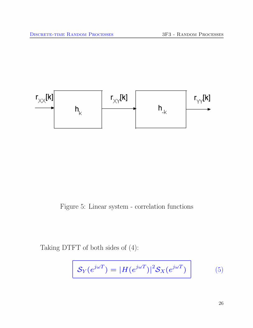
Discrete-time Random Processes 3F3 - Random Processes
Figure 5 Linear system - correlation functions
Taking DTFT of both sides of (4)
SY (ejωT
) = |H(ejωT
)|2SX(ejωT
) (5)
26
Discrete-time Random Processes 3F3 - Random Processes
Power spectrum at the output of a LTI system
27
Discrete-time Random Processes 3F3 - Random Processes
Example Filtering white noise
Suppose we filter a zero mean white noise process Xn with a first
order finite impulse response (FIR) filter
yn =1sum
m=0
bm xnminusm or Y (z) = (b0 + b1zminus1
)X(z)
with b0 = 1 b1 = 09 This an example of a moving average
(MA) process
The impulse response of this causal filter is
hn = b0 b1 0 0
The autocorrelation function of Yn is obtained as
rY Y [l] = E[Yn Yn+l] = hl lowast hminusl lowast rXX[l] (6)
This convolution can be performed directly However it is more
straightforward in the frequency domain
The frequency response of the filter is
H(ejΩ
) = b0 + b1eminusjΩ
28
Discrete-time Random Processes 3F3 - Random Processes
The power spectrum of Xn (white noise) is
SX(ejΩ
) = σ2X
Hence the power spectrum of Yn is
SY (ejΩ
) = |H(ejΩ
)|2SX(ejΩ
)
= |b0 + b1eminusjΩ|2σ2
X
= (b0b1e+jΩ
+ (b20 + b
21) + b0b1e
minusjΩ)σ
2X
as shown in the figure overleaf Comparing this expression with the
DTFT of rY Y [m]
SY (ejΩ
) =
infinsumm=minusinfin
rY Y [m] eminusjmΩ
we can identify non-zero terms in the summation only when m =
minus1 0+1 as follows
rY Y [minus1] = σ2Xb0b1 rY Y [0] = σ
2X(b
20 + b
21)
rY Y [1] = σ2Xb0b1
29
Discrete-time Random Processes 3F3 - Random Processes
Figure 6 Power spectrum of filtered white noise
30
Discrete-time Random Processes 3F3 - Random Processes
Ergodic Random processes
bull For an Ergodic random process we can estimate expectations
by performing time-averaging on a single sample function eg
micro = E[Xn] = limNrarrinfin
1
N
Nminus1sumn=0
xn (Mean ergodic)
rXX[k] = limNrarrinfin
1
N
Nminus1sumn=0
xnxn+k (Correlation ergodic) (7)
bull As in the continuous-time case these formulae allow us to make
the following estimates for lsquosufficientlyrsquo large N
micro = E[Xn] asymp1
N
Nminus1sumn=0
xn (Mean ergodic)
rXX[k] asymp1
N
Nminus1sumn=0
xnxn+k (Correlation ergodic) (8)
Note however that this is implemented with a simple computer
code loop in discrete-time unlike the continuous-time case
which requires an approximate integrator circuit
Under what conditions is a random process ergodic
31
Discrete-time Random Processes 3F3 - Random Processes
bull It is hard in general to determine whether a given process is
ergodic
bull A necessary and sufficient condition for mean ergodicity is given
by
limNrarrinfin
1
N
Nminus1sumk=0
cXX[k] = 0
where cXX is the autocovariance function
cXX[k] = E[(Xn minus micro)(Xn+k minus micro)]
and micro = E[Xn]
bull A simpler sufficient condition for mean ergodiciy is that
cXX[0] ltinfin and
limNrarrinfin
cXX[N ] = 0
bull Correlation ergodicity can be studied by extensions of the above
theorems We will not require the details here
bull Unless otherwise stated we will always assume that the signals
we encounter are both wide-sense stationary and ergodic
Although neither of these will always be true it will usually be
acceptable to assume so in practice
32
Discrete-time Random Processes 3F3 - Random Processes
Example
Consider the very simple lsquodc levelrsquo random process
Xn = A
where A is a random variable having the standard (ie mean zero
variance=1) Gaussian distribution
f(A) = N (A|0 1)
The mean of the random process is
E[Xn] =
int infinminusinfin
xn(a)f(a)da =
int infinminusinfin
af(a)da = 0
Now consider a random sample function measured from the random
process say
xt = a0
The mean value of this particular sample function is E[a0] = a0
Since in general a0 6= 0 the process is clearly not mean ergodic
33
Check this using the mean ergodic theorem The autocovariance
function is
cXX[k] = E[(Xn minus micro)(Xn+k minus micro)]
= E[XnXn+k] = E[A2] = 1
Now
limNrarrinfin
1
N
Nminus1sumk=0
cXX[k] = (1timesN)N = 1 6= 0
Hence the theorem confirms our finding that the process is not
ergodic in the mean
While this example highlights a possible pitfall in assuming
ergodicity most of the processes we deal with will however be
ergodic see examples paper for the random phase sine-wave and
the white noise processes
Comment Complex-valued processes
The above theory is easily extended to complex valued processes
Xn = XRen +jXIm
n in which case the autocorrelation function
is defined as
rXX[k] = E[XlowastnXn+k]
Revision Continuous time random processes
Figure 7 Ensemble representation of a random process
bull A random process is an ensemble of functions X(t) ω representingthe set of all possible waveforms that we might observe for that process
[NB ω is identical to the random variable α in the 3F1 notes]
ω is a random variable with its own probability distribution Pω whichdetermines randomly which waveform X(t ω) is observed ω may becontinuous- or discrete-valued
As before we will often omit ω and refer simply to random processX(t)
bull The mean of a random process is defined as micro(t) = E[X(t)] and theautocorrelation function as rXX [t1 t2] = E[X(t1)X(t2)] Theproperties of expectation allow us to calculate these in (at least) twoways
micro(t) = E[X(t1)]
=
intxx fX(t)(x) dx
=
intωX(t ω) fω(ω)dω
rXX(t1 t2) = E[X(t1)X(t2)]
=
intx1
intx2
x1x2 fX(t1)X(t2)(x1 x2) dx1dx2
=
intωX(t1 ω)X(t2 ω)fω(ω)dω
ie directly in terms of the density functions for X(t) or indirectly interms of the density function for ω
bull A wide-sense stationary (WSS) process X(t) is defined such that itsmean is a constant and rXX(t1 t2) depends only upon the differenceτ = t2 minus t1 ie
E[X(t)] = micro rXX(τ) = E[X(t)X(t+ τ)] (9)
[Wide-sense stationarity is also referred to as lsquoweak stationarityrsquo]
bull The Power Spectrum or Spectral Density of a WSS random process isdefined as the Fourier Transform of rXX(τ)
SX(ω) =
int infinminusinfin
rXX(τ) eminusjωτ
dτ (10)
bull For an Ergodic random process we can estimate expectations byperforming time-averaging on a single sample function eg
micro = E[X(t)] = limDrarrinfin
1
2D
int +D
minusDx(t)dt
rXX(τ) = limDrarrinfin
1
2D
int +D
minusDx(t)x(t+ τ)dt
Therefore for ergodic random processes we can make estimates forthese quantities by integrating over some suitably large (but finite) timeinterval 2D eg
E[X(t)] asymp1
2D
int +D
minusDx(t)dt
rXX(τ) asymp1
2D
int +D
minusDx(t)x(t+ τ)dt
where x(t) is a waveform measured at random from the process
Section 2 Optimal Filtering
Parts of this section and Section 3 are adapted from material kindly
supplied by Prof Peter Rayner
bull Optimal filtering is an area in which we design filters that are
optimally adapted to the statistical characteristics of a random
process As such the area can be seen as a combination of
standard filter design for deterministic signals with the random
process theory of the previous section
bull This remarkable area was pioneered in the 1940rsquos by Norbert
Wiener who designed methods for optimal estimation of a
signal measured in noise Specifically consider the system in the
figure below
Figure 8 The general Wiener filtering problem
bull A desired signal dn is observed in noise vn
xn = dn + vn
bull Wiener showed how to design a linear filter which would
optimally estimate dn given just the noisy observations xn and
some assumptions about the statistics of the random signal and
noise processes This class of filters the Wiener filter forms
the basis of many fundamental signal processing applications
bull Typical applications include
Noise reduction eg for speech and music signals
Prediction of future values of a signal eg in finance
Noise cancellation eg for aircraft cockpit noise
Deconvolution eg removal of room acoustics
(dereverberation) or echo cancellation in telephony
bull The Wiener filter is a very powerful tool However it is only the
optimal linear estimator for stationary signals The Kalman
filter offers an extension for non-stationary signals via state
space models In cases where a linear filter is still not good
enough non-linear filtering techniques can be adopted See 4th
year Signal Processing and Control modules for more advanced
topics in these areas
The Discrete-time Wiener Filter
In a minor abuse of notation and following standard conventions
we will refer to both random variables and their possible values in
lower-case symbols as this should cause no ambiguity for this section
of work
Figure 9 Wiener Filter
bull In the most general case we can filter the observed signal xnwith an Infinite impulse response (IIR) filter having a
non-causal impulse response hp
hp p = minusinfin minus1 0 1 2 infin (11)
bull We filter the observed noisy signal using the filter hp to
obtain an estimate dn of the desired signal
dn =infinsum
p=minusinfinhp xnminusp (12)
bull Since both dn and xn are drawn from random processes dnand xn we can only measure performance of the filter in
terms of expectations The criterion adopted for Wiener
filtering is the mean-squared error (MSE) criterion First
form the error signal εn
εn = dn minus dn = dn minusinfinsum
p=minusinfinhp xnminusp
The mean-squared error (MSE) is then defined as
J = E[ε2n] (13)
bull The Wiener filter minimises J with respect to the filter
coefficients hp
Derivation of Wiener filter
The Wiener filter assumes that xn and dn are jointly wide-
sense stationary This means that the means of both processes
are constant and all autocorrelation functionscross-correlation
functions (eg rxd[nm]) depend only on the time differencemminusnbetween data points
The expected error (13) may be minimised with respect to the
impulse response values hq A sufficient condition for a minimum
is
partJ
parthq=partE[ε2
n]
parthq= E
[partε2
n
parthq
]= E
[2εn
partεn
parthq
]= 0
for each q isin minusinfin minus1 0 1 2 infin
The term partεnparthq
is then calculated as
partεn
parthq=
part
parthq
dn minusinfinsum
p=minusinfinhp xnminusp
= minusxnminusq
and hence the coefficients must satisfy
E [εn xnminusq] = 0 minusinfin lt q lt +infin (14)
This is known as the orthogonality principle since two random
variables X and Y are termed orthogonal if
E[XY ] = 0
Now substituting for εn in (14) gives
E [εn xnminusq] = E
dn minus infinsump=minusinfin
hp xnminusp
xnminusq
= E [dn xnminusq]minus
infinsump=minusinfin
hp E [xnminusq xnminusp]
= rxd[q]minusinfinsum
p=minusinfinhp rxx[q minus p]
= 0
Hence rearranging the solution must satisfy
infinsump=minusinfin
hp rxx[q minus p] = rxd[q] minusinfin lt q lt +infin (15)
This is known as the Wiener-Hopf equations
The Wiener-Hopf equations involve an infinite number of unknowns
hq The simplest way to solve this is in the frequency domain First
note that the Wiener-Hopf equations can be rewritten as a discrete-
time convolution
hq lowast rxx[q] = rxd[q] minusinfin lt q lt +infin (16)
Taking discrete-time Fourier transforms (DTFT) of both sides
H(ejΩ
)Sx(ejΩ) = Sxd(ejΩ)
where Sxd(ejΩ) the DTFT of rxd[q] is defined as the cross-power
spectrum of d and x
Hence rearranging
H(ejΩ
) =Sxd(ejΩ)
Sx(ejΩ)(17)
Frequency domain Wiener filter
Mean-squared error for the optimal filter
The previous equations show how to calculate the optimal filter for
a given problem They donrsquot however tell us how well that optimal
filter performs This can be assessed from the mean-squared error
value of the optimal filter
J = E[ε2n] = E[εn(dn minus
infinsump=minusinfin
hp xnminusp)]
= E[εn dn]minusinfinsum
p=minusinfinhpE[εn xnminusp]
The expectation on the right is zero however for the optimal filter
by the orthogonality condition (14) so the minimum error is
Jmin = E[εn dn]
= E[(dn minusinfinsum
p=minusinfinhp xnminusp) dn]
= rdd[0]minusinfinsum
p=minusinfinhp rxd[p]
Important Special Case Uncorrelated Signal and Noise Processes
An important sub-class of the Wiener filter which also gives
considerable insight into filter behaviour can be gained by
considering the case where the desired signal process dn is
uncorrelated with the noise process vn ie
rdv[k] = E[dnvn+k] = 0 minusinfin lt k lt +infin
Consider the implications of this fact on the correlation functions
required in the Wiener-Hopf equations
infinsump=minusinfin
hp rxx[q minus p] = rxd[q] minusinfin lt q lt +infin
1 rxd
rxd[q] = E[xndn+q] = E[(dn + vn)dn+q] (18)
= E[dndn+q] + E[vndn+q] = rdd[q] (19)
since dn and vn are uncorrelated
Hence taking DTFT of both sides
Sxd(ejΩ) = Sd(ejΩ)
2 rxx
rxx[q] = E[xnxn+q] = E[(dn + vn)(dn+q + vn+q)]
= E[dndn+q] + E[vnvn+q] + E[dnvn+q] + E[vndn+q]
= E[dndn+q] + E[vnvn+q] = rdd[q] + rvv[q]
Hence
Sx(ejΩ) = Sd(ejΩ) + Sv(ejΩ)
Thus the Wiener filter becomes
H(ejΩ
) =Sd(ejΩ)
Sd(ejΩ) + Sv(ejΩ)
From this it can be seen that the behaviour of the filter is intuitively
reasonable in that at those frequencies where the noise power
spectrum Sv(ejΩ) is small the gain of the filter tends to unity
whereas the gain tends to a small value at those frequencies where the
noise spectrum is significantly larger than the desired signal power
spectrum Sd(ejΩ)
Example AR Process
An autoregressive process Dn of order 1 (see section 3) has power
spectrum
SD(ejΩ
) =σ2e
(1minus a1eminusjΩ)(1minus a1ejΩ)
Suppose the process is observed in zero mean white noise with
variance σ2v which is uncorrelated with Dn
xn = dn + vn
Design the Wiener filter for estimation of dn
Since the noise and desired signal are uncorrelated we can use the
form of Wiener filter from the previous page Substituting in the
various terms and rearranging its frequency response is
H(ejΩ
) =σ2e
σ2e + σ2
v(1minus a1eminusjΩ)(1minus a1ejΩ)
The impulse response of the filter can be found by inverse Fourier
transforming the frequency response This is studied in the examples
paper
The FIR Wiener filter
Note that in general the Wiener filter given by equation (17) is
non-causal and hence physically unrealisable in that the impulse
response hp is defined for values of p less than 0 Here we consider a
practical alternative in which a causal FIR Wiener filter is developed
In the FIR case the signal estimate is formed as
dn =
Pminus1sump=0
hp xnminusp (20)
and we minimise as before the objective function
J = E[(dn minus dn)2]
The filter derivation proceeds as before leading to an orthogonality
principle
E [εn xnminusq] = 0 q = 0 P minus 1 (21)
and Wiener-Hopf equations as follows
Pminus1sump=0
hp rxx[q minus p] = rxd[q] q = 0 1 P minus 1
(22)
The above equations may be written in matrix form as
Rxh = rxd
where
h =
h0
h1
hPminus1
rxd =
rxd[0]
rxd[1]
rxd[P minus 1]
and
Rx =
rxx[0] rxx[1] middot middot middot rxx[P minus 1]
rxx[1] rxx[0] rxx[P minus 2]
rxx[P minus 1] rxx[P minus 2] middot middot middot rxx[0]
Rx is known as the correlation matrix
Note that rxx[k] = rxx[minusk] so that the correlation matrix Rx
is symmetric and has constant diagonals (a symmetric Toeplitz
matrix)
The coefficient vector can be found by matrix inversion
h = Rxminus1
rxd (23)
This is the FIR Wiener filter and as for the general Wiener filter it
requires a-priori knowledge of the autocorrelation matrix Rx of the
input process xn and the cross-correlation rxd between the input
xn and the desired signal process dn
As before the minimum mean-squared error is given by
Jmin = E[εn dn]
= E[(dn minusPminus1sump=0
hp xnminusp) dn]
= rdd[0]minusPminus1sump=0
hp rxd[p]
= rdd[0]minus rTxdh = rdd[0]minus r
TxdRx
minus1rxd
Case Study Audio Noise Reduction
bull Consider a section of acoustic waveform (music voice ) dnthat is corrupted by additive noise vn
xn = dn + vn
bull We could try and noise reduce the signal using the FIR Wiener
filter
bull Assume that the section of data is wide-sense stationary and
ergodic (approx true for a short segment around 140 s)
Assume also that the noise is white and uncorrelated with the
audio signal - with variance σ2v ie
rvv[k] = σ2vδ[k]
Discrete-time Random Processes 3F3 - Random Processes
The power spectrum of Xn (white noise) is
SX(ejΩ
) = σ2X
Hence the power spectrum of Yn is
SY (ejΩ
) = |H(ejΩ
)|2SX(ejΩ
)
= |b0 + b1eminusjΩ|2σ2
X
= (b0b1e+jΩ
+ (b20 + b
21) + b0b1e
minusjΩ)σ
2X
as shown in the figure overleaf Comparing this expression with the
DTFT of rY Y [m]
SY (ejΩ
) =
infinsumm=minusinfin
rY Y [m] eminusjmΩ
we can identify non-zero terms in the summation only when m =
minus1 0+1 as follows
rY Y [minus1] = σ2Xb0b1 rY Y [0] = σ
2X(b
20 + b
21)
rY Y [1] = σ2Xb0b1
29
Discrete-time Random Processes 3F3 - Random Processes
Figure 6 Power spectrum of filtered white noise
30
Discrete-time Random Processes 3F3 - Random Processes
Ergodic Random processes
bull For an Ergodic random process we can estimate expectations
by performing time-averaging on a single sample function eg
micro = E[Xn] = limNrarrinfin
1
N
Nminus1sumn=0
xn (Mean ergodic)
rXX[k] = limNrarrinfin
1
N
Nminus1sumn=0
xnxn+k (Correlation ergodic) (7)
bull As in the continuous-time case these formulae allow us to make
the following estimates for lsquosufficientlyrsquo large N
micro = E[Xn] asymp1
N
Nminus1sumn=0
xn (Mean ergodic)
rXX[k] asymp1
N
Nminus1sumn=0
xnxn+k (Correlation ergodic) (8)
Note however that this is implemented with a simple computer
code loop in discrete-time unlike the continuous-time case
which requires an approximate integrator circuit
Under what conditions is a random process ergodic
31
Discrete-time Random Processes 3F3 - Random Processes
bull It is hard in general to determine whether a given process is
ergodic
bull A necessary and sufficient condition for mean ergodicity is given
by
limNrarrinfin
1
N
Nminus1sumk=0
cXX[k] = 0
where cXX is the autocovariance function
cXX[k] = E[(Xn minus micro)(Xn+k minus micro)]
and micro = E[Xn]
bull A simpler sufficient condition for mean ergodiciy is that
cXX[0] ltinfin and
limNrarrinfin
cXX[N ] = 0
bull Correlation ergodicity can be studied by extensions of the above
theorems We will not require the details here
bull Unless otherwise stated we will always assume that the signals
we encounter are both wide-sense stationary and ergodic
Although neither of these will always be true it will usually be
acceptable to assume so in practice
32
Discrete-time Random Processes 3F3 - Random Processes
Example
Consider the very simple lsquodc levelrsquo random process
Xn = A
where A is a random variable having the standard (ie mean zero
variance=1) Gaussian distribution
f(A) = N (A|0 1)
The mean of the random process is
E[Xn] =
int infinminusinfin
xn(a)f(a)da =
int infinminusinfin
af(a)da = 0
Now consider a random sample function measured from the random
process say
xt = a0
The mean value of this particular sample function is E[a0] = a0
Since in general a0 6= 0 the process is clearly not mean ergodic
33
Check this using the mean ergodic theorem The autocovariance
function is
cXX[k] = E[(Xn minus micro)(Xn+k minus micro)]
= E[XnXn+k] = E[A2] = 1
Now
limNrarrinfin
1
N
Nminus1sumk=0
cXX[k] = (1timesN)N = 1 6= 0
Hence the theorem confirms our finding that the process is not
ergodic in the mean
While this example highlights a possible pitfall in assuming
ergodicity most of the processes we deal with will however be
ergodic see examples paper for the random phase sine-wave and
the white noise processes
Comment Complex-valued processes
The above theory is easily extended to complex valued processes
Xn = XRen +jXIm
n in which case the autocorrelation function
is defined as
rXX[k] = E[XlowastnXn+k]
Revision Continuous time random processes
Figure 7 Ensemble representation of a random process
bull A random process is an ensemble of functions X(t) ω representingthe set of all possible waveforms that we might observe for that process
[NB ω is identical to the random variable α in the 3F1 notes]
ω is a random variable with its own probability distribution Pω whichdetermines randomly which waveform X(t ω) is observed ω may becontinuous- or discrete-valued
As before we will often omit ω and refer simply to random processX(t)
bull The mean of a random process is defined as micro(t) = E[X(t)] and theautocorrelation function as rXX [t1 t2] = E[X(t1)X(t2)] Theproperties of expectation allow us to calculate these in (at least) twoways
micro(t) = E[X(t1)]
=
intxx fX(t)(x) dx
=
intωX(t ω) fω(ω)dω
rXX(t1 t2) = E[X(t1)X(t2)]
=
intx1
intx2
x1x2 fX(t1)X(t2)(x1 x2) dx1dx2
=
intωX(t1 ω)X(t2 ω)fω(ω)dω
ie directly in terms of the density functions for X(t) or indirectly interms of the density function for ω
bull A wide-sense stationary (WSS) process X(t) is defined such that itsmean is a constant and rXX(t1 t2) depends only upon the differenceτ = t2 minus t1 ie
E[X(t)] = micro rXX(τ) = E[X(t)X(t+ τ)] (9)
[Wide-sense stationarity is also referred to as lsquoweak stationarityrsquo]
bull The Power Spectrum or Spectral Density of a WSS random process isdefined as the Fourier Transform of rXX(τ)
SX(ω) =
int infinminusinfin
rXX(τ) eminusjωτ
dτ (10)
bull For an Ergodic random process we can estimate expectations byperforming time-averaging on a single sample function eg
micro = E[X(t)] = limDrarrinfin
1
2D
int +D
minusDx(t)dt
rXX(τ) = limDrarrinfin
1
2D
int +D
minusDx(t)x(t+ τ)dt
Therefore for ergodic random processes we can make estimates forthese quantities by integrating over some suitably large (but finite) timeinterval 2D eg
E[X(t)] asymp1
2D
int +D
minusDx(t)dt
rXX(τ) asymp1
2D
int +D
minusDx(t)x(t+ τ)dt
where x(t) is a waveform measured at random from the process
Section 2 Optimal Filtering
Parts of this section and Section 3 are adapted from material kindly
supplied by Prof Peter Rayner
bull Optimal filtering is an area in which we design filters that are
optimally adapted to the statistical characteristics of a random
process As such the area can be seen as a combination of
standard filter design for deterministic signals with the random
process theory of the previous section
bull This remarkable area was pioneered in the 1940rsquos by Norbert
Wiener who designed methods for optimal estimation of a
signal measured in noise Specifically consider the system in the
figure below
Figure 8 The general Wiener filtering problem
bull A desired signal dn is observed in noise vn
xn = dn + vn
bull Wiener showed how to design a linear filter which would
optimally estimate dn given just the noisy observations xn and
some assumptions about the statistics of the random signal and
noise processes This class of filters the Wiener filter forms
the basis of many fundamental signal processing applications
bull Typical applications include
Noise reduction eg for speech and music signals
Prediction of future values of a signal eg in finance
Noise cancellation eg for aircraft cockpit noise
Deconvolution eg removal of room acoustics
(dereverberation) or echo cancellation in telephony
bull The Wiener filter is a very powerful tool However it is only the
optimal linear estimator for stationary signals The Kalman
filter offers an extension for non-stationary signals via state
space models In cases where a linear filter is still not good
enough non-linear filtering techniques can be adopted See 4th
year Signal Processing and Control modules for more advanced
topics in these areas
The Discrete-time Wiener Filter
In a minor abuse of notation and following standard conventions
we will refer to both random variables and their possible values in
lower-case symbols as this should cause no ambiguity for this section
of work
Figure 9 Wiener Filter
bull In the most general case we can filter the observed signal xnwith an Infinite impulse response (IIR) filter having a
non-causal impulse response hp
hp p = minusinfin minus1 0 1 2 infin (11)
bull We filter the observed noisy signal using the filter hp to
obtain an estimate dn of the desired signal
dn =infinsum
p=minusinfinhp xnminusp (12)
bull Since both dn and xn are drawn from random processes dnand xn we can only measure performance of the filter in
terms of expectations The criterion adopted for Wiener
filtering is the mean-squared error (MSE) criterion First
form the error signal εn
εn = dn minus dn = dn minusinfinsum
p=minusinfinhp xnminusp
The mean-squared error (MSE) is then defined as
J = E[ε2n] (13)
bull The Wiener filter minimises J with respect to the filter
coefficients hp
Derivation of Wiener filter
The Wiener filter assumes that xn and dn are jointly wide-
sense stationary This means that the means of both processes
are constant and all autocorrelation functionscross-correlation
functions (eg rxd[nm]) depend only on the time differencemminusnbetween data points
The expected error (13) may be minimised with respect to the
impulse response values hq A sufficient condition for a minimum
is
partJ
parthq=partE[ε2
n]
parthq= E
[partε2
n
parthq
]= E
[2εn
partεn
parthq
]= 0
for each q isin minusinfin minus1 0 1 2 infin
The term partεnparthq
is then calculated as
partεn
parthq=
part
parthq
dn minusinfinsum
p=minusinfinhp xnminusp
= minusxnminusq
and hence the coefficients must satisfy
E [εn xnminusq] = 0 minusinfin lt q lt +infin (14)
This is known as the orthogonality principle since two random
variables X and Y are termed orthogonal if
E[XY ] = 0
Now substituting for εn in (14) gives
E [εn xnminusq] = E
dn minus infinsump=minusinfin
hp xnminusp
xnminusq
= E [dn xnminusq]minus
infinsump=minusinfin
hp E [xnminusq xnminusp]
= rxd[q]minusinfinsum
p=minusinfinhp rxx[q minus p]
= 0
Hence rearranging the solution must satisfy
infinsump=minusinfin
hp rxx[q minus p] = rxd[q] minusinfin lt q lt +infin (15)
This is known as the Wiener-Hopf equations
The Wiener-Hopf equations involve an infinite number of unknowns
hq The simplest way to solve this is in the frequency domain First
note that the Wiener-Hopf equations can be rewritten as a discrete-
time convolution
hq lowast rxx[q] = rxd[q] minusinfin lt q lt +infin (16)
Taking discrete-time Fourier transforms (DTFT) of both sides
H(ejΩ
)Sx(ejΩ) = Sxd(ejΩ)
where Sxd(ejΩ) the DTFT of rxd[q] is defined as the cross-power
spectrum of d and x
Hence rearranging
H(ejΩ
) =Sxd(ejΩ)
Sx(ejΩ)(17)
Frequency domain Wiener filter
Mean-squared error for the optimal filter
The previous equations show how to calculate the optimal filter for
a given problem They donrsquot however tell us how well that optimal
filter performs This can be assessed from the mean-squared error
value of the optimal filter
J = E[ε2n] = E[εn(dn minus
infinsump=minusinfin
hp xnminusp)]
= E[εn dn]minusinfinsum
p=minusinfinhpE[εn xnminusp]
The expectation on the right is zero however for the optimal filter
by the orthogonality condition (14) so the minimum error is
Jmin = E[εn dn]
= E[(dn minusinfinsum
p=minusinfinhp xnminusp) dn]
= rdd[0]minusinfinsum
p=minusinfinhp rxd[p]
Important Special Case Uncorrelated Signal and Noise Processes
An important sub-class of the Wiener filter which also gives
considerable insight into filter behaviour can be gained by
considering the case where the desired signal process dn is
uncorrelated with the noise process vn ie
rdv[k] = E[dnvn+k] = 0 minusinfin lt k lt +infin
Consider the implications of this fact on the correlation functions
required in the Wiener-Hopf equations
infinsump=minusinfin
hp rxx[q minus p] = rxd[q] minusinfin lt q lt +infin
1 rxd
rxd[q] = E[xndn+q] = E[(dn + vn)dn+q] (18)
= E[dndn+q] + E[vndn+q] = rdd[q] (19)
since dn and vn are uncorrelated
Hence taking DTFT of both sides
Sxd(ejΩ) = Sd(ejΩ)
2 rxx
rxx[q] = E[xnxn+q] = E[(dn + vn)(dn+q + vn+q)]
= E[dndn+q] + E[vnvn+q] + E[dnvn+q] + E[vndn+q]
= E[dndn+q] + E[vnvn+q] = rdd[q] + rvv[q]
Hence
Sx(ejΩ) = Sd(ejΩ) + Sv(ejΩ)
Thus the Wiener filter becomes
H(ejΩ
) =Sd(ejΩ)
Sd(ejΩ) + Sv(ejΩ)
From this it can be seen that the behaviour of the filter is intuitively
reasonable in that at those frequencies where the noise power
spectrum Sv(ejΩ) is small the gain of the filter tends to unity
whereas the gain tends to a small value at those frequencies where the
noise spectrum is significantly larger than the desired signal power
spectrum Sd(ejΩ)
Example AR Process
An autoregressive process Dn of order 1 (see section 3) has power
spectrum
SD(ejΩ
) =σ2e
(1minus a1eminusjΩ)(1minus a1ejΩ)
Suppose the process is observed in zero mean white noise with
variance σ2v which is uncorrelated with Dn
xn = dn + vn
Design the Wiener filter for estimation of dn
Since the noise and desired signal are uncorrelated we can use the
form of Wiener filter from the previous page Substituting in the
various terms and rearranging its frequency response is
H(ejΩ
) =σ2e
σ2e + σ2
v(1minus a1eminusjΩ)(1minus a1ejΩ)
The impulse response of the filter can be found by inverse Fourier
transforming the frequency response This is studied in the examples
paper
The FIR Wiener filter
Note that in general the Wiener filter given by equation (17) is
non-causal and hence physically unrealisable in that the impulse
response hp is defined for values of p less than 0 Here we consider a
practical alternative in which a causal FIR Wiener filter is developed
In the FIR case the signal estimate is formed as
dn =
Pminus1sump=0
hp xnminusp (20)
and we minimise as before the objective function
J = E[(dn minus dn)2]
The filter derivation proceeds as before leading to an orthogonality
principle
E [εn xnminusq] = 0 q = 0 P minus 1 (21)
and Wiener-Hopf equations as follows
Pminus1sump=0
hp rxx[q minus p] = rxd[q] q = 0 1 P minus 1
(22)
The above equations may be written in matrix form as
Rxh = rxd
where
h =
h0
h1
hPminus1
rxd =
rxd[0]
rxd[1]
rxd[P minus 1]
and
Rx =
rxx[0] rxx[1] middot middot middot rxx[P minus 1]
rxx[1] rxx[0] rxx[P minus 2]
rxx[P minus 1] rxx[P minus 2] middot middot middot rxx[0]
Rx is known as the correlation matrix
Note that rxx[k] = rxx[minusk] so that the correlation matrix Rx
is symmetric and has constant diagonals (a symmetric Toeplitz
matrix)
The coefficient vector can be found by matrix inversion
h = Rxminus1
rxd (23)
This is the FIR Wiener filter and as for the general Wiener filter it
requires a-priori knowledge of the autocorrelation matrix Rx of the
input process xn and the cross-correlation rxd between the input
xn and the desired signal process dn
As before the minimum mean-squared error is given by
Jmin = E[εn dn]
= E[(dn minusPminus1sump=0
hp xnminusp) dn]
= rdd[0]minusPminus1sump=0
hp rxd[p]
= rdd[0]minus rTxdh = rdd[0]minus r
TxdRx
minus1rxd
Case Study Audio Noise Reduction
bull Consider a section of acoustic waveform (music voice ) dnthat is corrupted by additive noise vn
xn = dn + vn
bull We could try and noise reduce the signal using the FIR Wiener
filter
bull Assume that the section of data is wide-sense stationary and
ergodic (approx true for a short segment around 140 s)
Assume also that the noise is white and uncorrelated with the
audio signal - with variance σ2v ie
rvv[k] = σ2vδ[k]
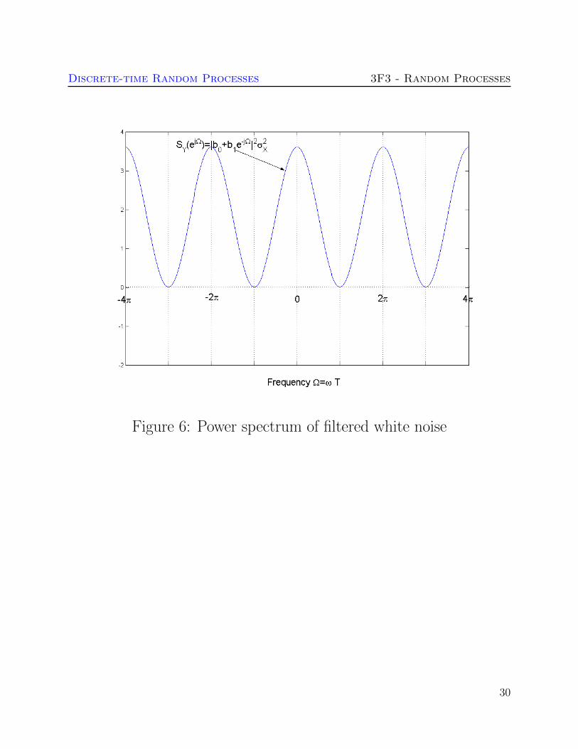
Discrete-time Random Processes 3F3 - Random Processes
Figure 6 Power spectrum of filtered white noise
30
Discrete-time Random Processes 3F3 - Random Processes
Ergodic Random processes
bull For an Ergodic random process we can estimate expectations
by performing time-averaging on a single sample function eg
micro = E[Xn] = limNrarrinfin
1
N
Nminus1sumn=0
xn (Mean ergodic)
rXX[k] = limNrarrinfin
1
N
Nminus1sumn=0
xnxn+k (Correlation ergodic) (7)
bull As in the continuous-time case these formulae allow us to make
the following estimates for lsquosufficientlyrsquo large N
micro = E[Xn] asymp1
N
Nminus1sumn=0
xn (Mean ergodic)
rXX[k] asymp1
N
Nminus1sumn=0
xnxn+k (Correlation ergodic) (8)
Note however that this is implemented with a simple computer
code loop in discrete-time unlike the continuous-time case
which requires an approximate integrator circuit
Under what conditions is a random process ergodic
31
Discrete-time Random Processes 3F3 - Random Processes
bull It is hard in general to determine whether a given process is
ergodic
bull A necessary and sufficient condition for mean ergodicity is given
by
limNrarrinfin
1
N
Nminus1sumk=0
cXX[k] = 0
where cXX is the autocovariance function
cXX[k] = E[(Xn minus micro)(Xn+k minus micro)]
and micro = E[Xn]
bull A simpler sufficient condition for mean ergodiciy is that
cXX[0] ltinfin and
limNrarrinfin
cXX[N ] = 0
bull Correlation ergodicity can be studied by extensions of the above
theorems We will not require the details here
bull Unless otherwise stated we will always assume that the signals
we encounter are both wide-sense stationary and ergodic
Although neither of these will always be true it will usually be
acceptable to assume so in practice
32
Discrete-time Random Processes 3F3 - Random Processes
Example
Consider the very simple lsquodc levelrsquo random process
Xn = A
where A is a random variable having the standard (ie mean zero
variance=1) Gaussian distribution
f(A) = N (A|0 1)
The mean of the random process is
E[Xn] =
int infinminusinfin
xn(a)f(a)da =
int infinminusinfin
af(a)da = 0
Now consider a random sample function measured from the random
process say
xt = a0
The mean value of this particular sample function is E[a0] = a0
Since in general a0 6= 0 the process is clearly not mean ergodic
33
Check this using the mean ergodic theorem The autocovariance
function is
cXX[k] = E[(Xn minus micro)(Xn+k minus micro)]
= E[XnXn+k] = E[A2] = 1
Now
limNrarrinfin
1
N
Nminus1sumk=0
cXX[k] = (1timesN)N = 1 6= 0
Hence the theorem confirms our finding that the process is not
ergodic in the mean
While this example highlights a possible pitfall in assuming
ergodicity most of the processes we deal with will however be
ergodic see examples paper for the random phase sine-wave and
the white noise processes
Comment Complex-valued processes
The above theory is easily extended to complex valued processes
Xn = XRen +jXIm
n in which case the autocorrelation function
is defined as
rXX[k] = E[XlowastnXn+k]
Revision Continuous time random processes
Figure 7 Ensemble representation of a random process
bull A random process is an ensemble of functions X(t) ω representingthe set of all possible waveforms that we might observe for that process
[NB ω is identical to the random variable α in the 3F1 notes]
ω is a random variable with its own probability distribution Pω whichdetermines randomly which waveform X(t ω) is observed ω may becontinuous- or discrete-valued
As before we will often omit ω and refer simply to random processX(t)
bull The mean of a random process is defined as micro(t) = E[X(t)] and theautocorrelation function as rXX [t1 t2] = E[X(t1)X(t2)] Theproperties of expectation allow us to calculate these in (at least) twoways
micro(t) = E[X(t1)]
=
intxx fX(t)(x) dx
=
intωX(t ω) fω(ω)dω
rXX(t1 t2) = E[X(t1)X(t2)]
=
intx1
intx2
x1x2 fX(t1)X(t2)(x1 x2) dx1dx2
=
intωX(t1 ω)X(t2 ω)fω(ω)dω
ie directly in terms of the density functions for X(t) or indirectly interms of the density function for ω
bull A wide-sense stationary (WSS) process X(t) is defined such that itsmean is a constant and rXX(t1 t2) depends only upon the differenceτ = t2 minus t1 ie
E[X(t)] = micro rXX(τ) = E[X(t)X(t+ τ)] (9)
[Wide-sense stationarity is also referred to as lsquoweak stationarityrsquo]
bull The Power Spectrum or Spectral Density of a WSS random process isdefined as the Fourier Transform of rXX(τ)
SX(ω) =
int infinminusinfin
rXX(τ) eminusjωτ
dτ (10)
bull For an Ergodic random process we can estimate expectations byperforming time-averaging on a single sample function eg
micro = E[X(t)] = limDrarrinfin
1
2D
int +D
minusDx(t)dt
rXX(τ) = limDrarrinfin
1
2D
int +D
minusDx(t)x(t+ τ)dt
Therefore for ergodic random processes we can make estimates forthese quantities by integrating over some suitably large (but finite) timeinterval 2D eg
E[X(t)] asymp1
2D
int +D
minusDx(t)dt
rXX(τ) asymp1
2D
int +D
minusDx(t)x(t+ τ)dt
where x(t) is a waveform measured at random from the process
Section 2 Optimal Filtering
Parts of this section and Section 3 are adapted from material kindly
supplied by Prof Peter Rayner
bull Optimal filtering is an area in which we design filters that are
optimally adapted to the statistical characteristics of a random
process As such the area can be seen as a combination of
standard filter design for deterministic signals with the random
process theory of the previous section
bull This remarkable area was pioneered in the 1940rsquos by Norbert
Wiener who designed methods for optimal estimation of a
signal measured in noise Specifically consider the system in the
figure below
Figure 8 The general Wiener filtering problem
bull A desired signal dn is observed in noise vn
xn = dn + vn
bull Wiener showed how to design a linear filter which would
optimally estimate dn given just the noisy observations xn and
some assumptions about the statistics of the random signal and
noise processes This class of filters the Wiener filter forms
the basis of many fundamental signal processing applications
bull Typical applications include
Noise reduction eg for speech and music signals
Prediction of future values of a signal eg in finance
Noise cancellation eg for aircraft cockpit noise
Deconvolution eg removal of room acoustics
(dereverberation) or echo cancellation in telephony
bull The Wiener filter is a very powerful tool However it is only the
optimal linear estimator for stationary signals The Kalman
filter offers an extension for non-stationary signals via state
space models In cases where a linear filter is still not good
enough non-linear filtering techniques can be adopted See 4th
year Signal Processing and Control modules for more advanced
topics in these areas
The Discrete-time Wiener Filter
In a minor abuse of notation and following standard conventions
we will refer to both random variables and their possible values in
lower-case symbols as this should cause no ambiguity for this section
of work
Figure 9 Wiener Filter
bull In the most general case we can filter the observed signal xnwith an Infinite impulse response (IIR) filter having a
non-causal impulse response hp
hp p = minusinfin minus1 0 1 2 infin (11)
bull We filter the observed noisy signal using the filter hp to
obtain an estimate dn of the desired signal
dn =infinsum
p=minusinfinhp xnminusp (12)
bull Since both dn and xn are drawn from random processes dnand xn we can only measure performance of the filter in
terms of expectations The criterion adopted for Wiener
filtering is the mean-squared error (MSE) criterion First
form the error signal εn
εn = dn minus dn = dn minusinfinsum
p=minusinfinhp xnminusp
The mean-squared error (MSE) is then defined as
J = E[ε2n] (13)
bull The Wiener filter minimises J with respect to the filter
coefficients hp
Derivation of Wiener filter
The Wiener filter assumes that xn and dn are jointly wide-
sense stationary This means that the means of both processes
are constant and all autocorrelation functionscross-correlation
functions (eg rxd[nm]) depend only on the time differencemminusnbetween data points
The expected error (13) may be minimised with respect to the
impulse response values hq A sufficient condition for a minimum
is
partJ
parthq=partE[ε2
n]
parthq= E
[partε2
n
parthq
]= E
[2εn
partεn
parthq
]= 0
for each q isin minusinfin minus1 0 1 2 infin
The term partεnparthq
is then calculated as
partεn
parthq=
part
parthq
dn minusinfinsum
p=minusinfinhp xnminusp
= minusxnminusq
and hence the coefficients must satisfy
E [εn xnminusq] = 0 minusinfin lt q lt +infin (14)
This is known as the orthogonality principle since two random
variables X and Y are termed orthogonal if
E[XY ] = 0
Now substituting for εn in (14) gives
E [εn xnminusq] = E
dn minus infinsump=minusinfin
hp xnminusp
xnminusq
= E [dn xnminusq]minus
infinsump=minusinfin
hp E [xnminusq xnminusp]
= rxd[q]minusinfinsum
p=minusinfinhp rxx[q minus p]
= 0
Hence rearranging the solution must satisfy
infinsump=minusinfin
hp rxx[q minus p] = rxd[q] minusinfin lt q lt +infin (15)
This is known as the Wiener-Hopf equations
The Wiener-Hopf equations involve an infinite number of unknowns
hq The simplest way to solve this is in the frequency domain First
note that the Wiener-Hopf equations can be rewritten as a discrete-
time convolution
hq lowast rxx[q] = rxd[q] minusinfin lt q lt +infin (16)
Taking discrete-time Fourier transforms (DTFT) of both sides
H(ejΩ
)Sx(ejΩ) = Sxd(ejΩ)
where Sxd(ejΩ) the DTFT of rxd[q] is defined as the cross-power
spectrum of d and x
Hence rearranging
H(ejΩ
) =Sxd(ejΩ)
Sx(ejΩ)(17)
Frequency domain Wiener filter
Mean-squared error for the optimal filter
The previous equations show how to calculate the optimal filter for
a given problem They donrsquot however tell us how well that optimal
filter performs This can be assessed from the mean-squared error
value of the optimal filter
J = E[ε2n] = E[εn(dn minus
infinsump=minusinfin
hp xnminusp)]
= E[εn dn]minusinfinsum
p=minusinfinhpE[εn xnminusp]
The expectation on the right is zero however for the optimal filter
by the orthogonality condition (14) so the minimum error is
Jmin = E[εn dn]
= E[(dn minusinfinsum
p=minusinfinhp xnminusp) dn]
= rdd[0]minusinfinsum
p=minusinfinhp rxd[p]
Important Special Case Uncorrelated Signal and Noise Processes
An important sub-class of the Wiener filter which also gives
considerable insight into filter behaviour can be gained by
considering the case where the desired signal process dn is
uncorrelated with the noise process vn ie
rdv[k] = E[dnvn+k] = 0 minusinfin lt k lt +infin
Consider the implications of this fact on the correlation functions
required in the Wiener-Hopf equations
infinsump=minusinfin
hp rxx[q minus p] = rxd[q] minusinfin lt q lt +infin
1 rxd
rxd[q] = E[xndn+q] = E[(dn + vn)dn+q] (18)
= E[dndn+q] + E[vndn+q] = rdd[q] (19)
since dn and vn are uncorrelated
Hence taking DTFT of both sides
Sxd(ejΩ) = Sd(ejΩ)
2 rxx
rxx[q] = E[xnxn+q] = E[(dn + vn)(dn+q + vn+q)]
= E[dndn+q] + E[vnvn+q] + E[dnvn+q] + E[vndn+q]
= E[dndn+q] + E[vnvn+q] = rdd[q] + rvv[q]
Hence
Sx(ejΩ) = Sd(ejΩ) + Sv(ejΩ)
Thus the Wiener filter becomes
H(ejΩ
) =Sd(ejΩ)
Sd(ejΩ) + Sv(ejΩ)
From this it can be seen that the behaviour of the filter is intuitively
reasonable in that at those frequencies where the noise power
spectrum Sv(ejΩ) is small the gain of the filter tends to unity
whereas the gain tends to a small value at those frequencies where the
noise spectrum is significantly larger than the desired signal power
spectrum Sd(ejΩ)
Example AR Process
An autoregressive process Dn of order 1 (see section 3) has power
spectrum
SD(ejΩ
) =σ2e
(1minus a1eminusjΩ)(1minus a1ejΩ)
Suppose the process is observed in zero mean white noise with
variance σ2v which is uncorrelated with Dn
xn = dn + vn
Design the Wiener filter for estimation of dn
Since the noise and desired signal are uncorrelated we can use the
form of Wiener filter from the previous page Substituting in the
various terms and rearranging its frequency response is
H(ejΩ
) =σ2e
σ2e + σ2
v(1minus a1eminusjΩ)(1minus a1ejΩ)
The impulse response of the filter can be found by inverse Fourier
transforming the frequency response This is studied in the examples
paper
The FIR Wiener filter
Note that in general the Wiener filter given by equation (17) is
non-causal and hence physically unrealisable in that the impulse
response hp is defined for values of p less than 0 Here we consider a
practical alternative in which a causal FIR Wiener filter is developed
In the FIR case the signal estimate is formed as
dn =
Pminus1sump=0
hp xnminusp (20)
and we minimise as before the objective function
J = E[(dn minus dn)2]
The filter derivation proceeds as before leading to an orthogonality
principle
E [εn xnminusq] = 0 q = 0 P minus 1 (21)
and Wiener-Hopf equations as follows
Pminus1sump=0
hp rxx[q minus p] = rxd[q] q = 0 1 P minus 1
(22)
The above equations may be written in matrix form as
Rxh = rxd
where
h =
h0
h1
hPminus1
rxd =
rxd[0]
rxd[1]
rxd[P minus 1]
and
Rx =
rxx[0] rxx[1] middot middot middot rxx[P minus 1]
rxx[1] rxx[0] rxx[P minus 2]
rxx[P minus 1] rxx[P minus 2] middot middot middot rxx[0]
Rx is known as the correlation matrix
Note that rxx[k] = rxx[minusk] so that the correlation matrix Rx
is symmetric and has constant diagonals (a symmetric Toeplitz
matrix)
The coefficient vector can be found by matrix inversion
h = Rxminus1
rxd (23)
This is the FIR Wiener filter and as for the general Wiener filter it
requires a-priori knowledge of the autocorrelation matrix Rx of the
input process xn and the cross-correlation rxd between the input
xn and the desired signal process dn
As before the minimum mean-squared error is given by
Jmin = E[εn dn]
= E[(dn minusPminus1sump=0
hp xnminusp) dn]
= rdd[0]minusPminus1sump=0
hp rxd[p]
= rdd[0]minus rTxdh = rdd[0]minus r
TxdRx
minus1rxd
Case Study Audio Noise Reduction
bull Consider a section of acoustic waveform (music voice ) dnthat is corrupted by additive noise vn
xn = dn + vn
bull We could try and noise reduce the signal using the FIR Wiener
filter
bull Assume that the section of data is wide-sense stationary and
ergodic (approx true for a short segment around 140 s)
Assume also that the noise is white and uncorrelated with the
audio signal - with variance σ2v ie
rvv[k] = σ2vδ[k]
Discrete-time Random Processes 3F3 - Random Processes
Example
Consider the very simple lsquodc levelrsquo random process
Xn = A
where A is a random variable having the standard (ie mean zero
variance=1) Gaussian distribution
f(A) = N (A|0 1)
The mean of the random process is
E[Xn] =
int infinminusinfin
xn(a)f(a)da =
int infinminusinfin
af(a)da = 0
Now consider a random sample function measured from the random
process say
xt = a0
The mean value of this particular sample function is E[a0] = a0
Since in general a0 6= 0 the process is clearly not mean ergodic
33
Check this using the mean ergodic theorem The autocovariance
function is
cXX[k] = E[(Xn minus micro)(Xn+k minus micro)]
= E[XnXn+k] = E[A2] = 1
Now
limNrarrinfin
1
N
Nminus1sumk=0
cXX[k] = (1timesN)N = 1 6= 0
Hence the theorem confirms our finding that the process is not
ergodic in the mean
While this example highlights a possible pitfall in assuming
ergodicity most of the processes we deal with will however be
ergodic see examples paper for the random phase sine-wave and
the white noise processes
Comment Complex-valued processes
The above theory is easily extended to complex valued processes
Xn = XRen +jXIm
n in which case the autocorrelation function
is defined as
rXX[k] = E[XlowastnXn+k]
Revision Continuous time random processes
Figure 7 Ensemble representation of a random process
bull A random process is an ensemble of functions X(t) ω representingthe set of all possible waveforms that we might observe for that process
[NB ω is identical to the random variable α in the 3F1 notes]
ω is a random variable with its own probability distribution Pω whichdetermines randomly which waveform X(t ω) is observed ω may becontinuous- or discrete-valued
As before we will often omit ω and refer simply to random processX(t)
bull The mean of a random process is defined as micro(t) = E[X(t)] and theautocorrelation function as rXX [t1 t2] = E[X(t1)X(t2)] Theproperties of expectation allow us to calculate these in (at least) twoways
micro(t) = E[X(t1)]
=
intxx fX(t)(x) dx
=
intωX(t ω) fω(ω)dω
rXX(t1 t2) = E[X(t1)X(t2)]
=
intx1
intx2
x1x2 fX(t1)X(t2)(x1 x2) dx1dx2
=
intωX(t1 ω)X(t2 ω)fω(ω)dω
ie directly in terms of the density functions for X(t) or indirectly interms of the density function for ω
bull A wide-sense stationary (WSS) process X(t) is defined such that itsmean is a constant and rXX(t1 t2) depends only upon the differenceτ = t2 minus t1 ie
E[X(t)] = micro rXX(τ) = E[X(t)X(t+ τ)] (9)
[Wide-sense stationarity is also referred to as lsquoweak stationarityrsquo]
bull The Power Spectrum or Spectral Density of a WSS random process isdefined as the Fourier Transform of rXX(τ)
SX(ω) =
int infinminusinfin
rXX(τ) eminusjωτ
dτ (10)
bull For an Ergodic random process we can estimate expectations byperforming time-averaging on a single sample function eg
micro = E[X(t)] = limDrarrinfin
1
2D
int +D
minusDx(t)dt
rXX(τ) = limDrarrinfin
1
2D
int +D
minusDx(t)x(t+ τ)dt
Therefore for ergodic random processes we can make estimates forthese quantities by integrating over some suitably large (but finite) timeinterval 2D eg
E[X(t)] asymp1
2D
int +D
minusDx(t)dt
rXX(τ) asymp1
2D
int +D
minusDx(t)x(t+ τ)dt
where x(t) is a waveform measured at random from the process
Section 2 Optimal Filtering
Parts of this section and Section 3 are adapted from material kindly
supplied by Prof Peter Rayner
bull Optimal filtering is an area in which we design filters that are
optimally adapted to the statistical characteristics of a random
process As such the area can be seen as a combination of
standard filter design for deterministic signals with the random
process theory of the previous section
bull This remarkable area was pioneered in the 1940rsquos by Norbert
Wiener who designed methods for optimal estimation of a
signal measured in noise Specifically consider the system in the
figure below
Figure 8 The general Wiener filtering problem
bull A desired signal dn is observed in noise vn
xn = dn + vn
bull Wiener showed how to design a linear filter which would
optimally estimate dn given just the noisy observations xn and
some assumptions about the statistics of the random signal and
noise processes This class of filters the Wiener filter forms
the basis of many fundamental signal processing applications
bull Typical applications include
Noise reduction eg for speech and music signals
Prediction of future values of a signal eg in finance
Noise cancellation eg for aircraft cockpit noise
Deconvolution eg removal of room acoustics
(dereverberation) or echo cancellation in telephony
bull The Wiener filter is a very powerful tool However it is only the
optimal linear estimator for stationary signals The Kalman
filter offers an extension for non-stationary signals via state
space models In cases where a linear filter is still not good
enough non-linear filtering techniques can be adopted See 4th
year Signal Processing and Control modules for more advanced
topics in these areas
The Discrete-time Wiener Filter
In a minor abuse of notation and following standard conventions
we will refer to both random variables and their possible values in
lower-case symbols as this should cause no ambiguity for this section
of work
Figure 9 Wiener Filter
bull In the most general case we can filter the observed signal xnwith an Infinite impulse response (IIR) filter having a
non-causal impulse response hp
hp p = minusinfin minus1 0 1 2 infin (11)
bull We filter the observed noisy signal using the filter hp to
obtain an estimate dn of the desired signal
dn =infinsum
p=minusinfinhp xnminusp (12)
bull Since both dn and xn are drawn from random processes dnand xn we can only measure performance of the filter in
terms of expectations The criterion adopted for Wiener
filtering is the mean-squared error (MSE) criterion First
form the error signal εn
εn = dn minus dn = dn minusinfinsum
p=minusinfinhp xnminusp
The mean-squared error (MSE) is then defined as
J = E[ε2n] (13)
bull The Wiener filter minimises J with respect to the filter
coefficients hp
Derivation of Wiener filter
The Wiener filter assumes that xn and dn are jointly wide-
sense stationary This means that the means of both processes
are constant and all autocorrelation functionscross-correlation
functions (eg rxd[nm]) depend only on the time differencemminusnbetween data points
The expected error (13) may be minimised with respect to the
impulse response values hq A sufficient condition for a minimum
is
partJ
parthq=partE[ε2
n]
parthq= E
[partε2
n
parthq
]= E
[2εn
partεn
parthq
]= 0
for each q isin minusinfin minus1 0 1 2 infin
The term partεnparthq
is then calculated as
partεn
parthq=
part
parthq
dn minusinfinsum
p=minusinfinhp xnminusp
= minusxnminusq
and hence the coefficients must satisfy
E [εn xnminusq] = 0 minusinfin lt q lt +infin (14)
This is known as the orthogonality principle since two random
variables X and Y are termed orthogonal if
E[XY ] = 0
Now substituting for εn in (14) gives
E [εn xnminusq] = E
dn minus infinsump=minusinfin
hp xnminusp
xnminusq
= E [dn xnminusq]minus
infinsump=minusinfin
hp E [xnminusq xnminusp]
= rxd[q]minusinfinsum
p=minusinfinhp rxx[q minus p]
= 0
Hence rearranging the solution must satisfy
infinsump=minusinfin
hp rxx[q minus p] = rxd[q] minusinfin lt q lt +infin (15)
This is known as the Wiener-Hopf equations
The Wiener-Hopf equations involve an infinite number of unknowns
hq The simplest way to solve this is in the frequency domain First
note that the Wiener-Hopf equations can be rewritten as a discrete-
time convolution
hq lowast rxx[q] = rxd[q] minusinfin lt q lt +infin (16)
Taking discrete-time Fourier transforms (DTFT) of both sides
H(ejΩ
)Sx(ejΩ) = Sxd(ejΩ)
where Sxd(ejΩ) the DTFT of rxd[q] is defined as the cross-power
spectrum of d and x
Hence rearranging
H(ejΩ
) =Sxd(ejΩ)
Sx(ejΩ)(17)
Frequency domain Wiener filter
Mean-squared error for the optimal filter
The previous equations show how to calculate the optimal filter for
a given problem They donrsquot however tell us how well that optimal
filter performs This can be assessed from the mean-squared error
value of the optimal filter
J = E[ε2n] = E[εn(dn minus
infinsump=minusinfin
hp xnminusp)]
= E[εn dn]minusinfinsum
p=minusinfinhpE[εn xnminusp]
The expectation on the right is zero however for the optimal filter
by the orthogonality condition (14) so the minimum error is
Jmin = E[εn dn]
= E[(dn minusinfinsum
p=minusinfinhp xnminusp) dn]
= rdd[0]minusinfinsum
p=minusinfinhp rxd[p]
Important Special Case Uncorrelated Signal and Noise Processes
An important sub-class of the Wiener filter which also gives
considerable insight into filter behaviour can be gained by
considering the case where the desired signal process dn is
uncorrelated with the noise process vn ie
rdv[k] = E[dnvn+k] = 0 minusinfin lt k lt +infin
Consider the implications of this fact on the correlation functions
required in the Wiener-Hopf equations
infinsump=minusinfin
hp rxx[q minus p] = rxd[q] minusinfin lt q lt +infin
1 rxd
rxd[q] = E[xndn+q] = E[(dn + vn)dn+q] (18)
= E[dndn+q] + E[vndn+q] = rdd[q] (19)
since dn and vn are uncorrelated
Hence taking DTFT of both sides
Sxd(ejΩ) = Sd(ejΩ)
2 rxx
rxx[q] = E[xnxn+q] = E[(dn + vn)(dn+q + vn+q)]
= E[dndn+q] + E[vnvn+q] + E[dnvn+q] + E[vndn+q]
= E[dndn+q] + E[vnvn+q] = rdd[q] + rvv[q]
Hence
Sx(ejΩ) = Sd(ejΩ) + Sv(ejΩ)
Thus the Wiener filter becomes
H(ejΩ
) =Sd(ejΩ)
Sd(ejΩ) + Sv(ejΩ)
From this it can be seen that the behaviour of the filter is intuitively
reasonable in that at those frequencies where the noise power
spectrum Sv(ejΩ) is small the gain of the filter tends to unity
whereas the gain tends to a small value at those frequencies where the
noise spectrum is significantly larger than the desired signal power
spectrum Sd(ejΩ)
Example AR Process
An autoregressive process Dn of order 1 (see section 3) has power
spectrum
SD(ejΩ
) =σ2e
(1minus a1eminusjΩ)(1minus a1ejΩ)
Suppose the process is observed in zero mean white noise with
variance σ2v which is uncorrelated with Dn
xn = dn + vn
Design the Wiener filter for estimation of dn
Since the noise and desired signal are uncorrelated we can use the
form of Wiener filter from the previous page Substituting in the
various terms and rearranging its frequency response is
H(ejΩ
) =σ2e
σ2e + σ2
v(1minus a1eminusjΩ)(1minus a1ejΩ)
The impulse response of the filter can be found by inverse Fourier
transforming the frequency response This is studied in the examples
paper
The FIR Wiener filter
Note that in general the Wiener filter given by equation (17) is
non-causal and hence physically unrealisable in that the impulse
response hp is defined for values of p less than 0 Here we consider a
practical alternative in which a causal FIR Wiener filter is developed
In the FIR case the signal estimate is formed as
dn =
Pminus1sump=0
hp xnminusp (20)
and we minimise as before the objective function
J = E[(dn minus dn)2]
The filter derivation proceeds as before leading to an orthogonality
principle
E [εn xnminusq] = 0 q = 0 P minus 1 (21)
and Wiener-Hopf equations as follows
Pminus1sump=0
hp rxx[q minus p] = rxd[q] q = 0 1 P minus 1
(22)
The above equations may be written in matrix form as
Rxh = rxd
where
h =
h0
h1
hPminus1
rxd =
rxd[0]
rxd[1]
rxd[P minus 1]
and
Rx =
rxx[0] rxx[1] middot middot middot rxx[P minus 1]
rxx[1] rxx[0] rxx[P minus 2]
rxx[P minus 1] rxx[P minus 2] middot middot middot rxx[0]
Rx is known as the correlation matrix
Note that rxx[k] = rxx[minusk] so that the correlation matrix Rx
is symmetric and has constant diagonals (a symmetric Toeplitz
matrix)
The coefficient vector can be found by matrix inversion
h = Rxminus1
rxd (23)
This is the FIR Wiener filter and as for the general Wiener filter it
requires a-priori knowledge of the autocorrelation matrix Rx of the
input process xn and the cross-correlation rxd between the input
xn and the desired signal process dn
As before the minimum mean-squared error is given by
Jmin = E[εn dn]
= E[(dn minusPminus1sump=0
hp xnminusp) dn]
= rdd[0]minusPminus1sump=0
hp rxd[p]
= rdd[0]minus rTxdh = rdd[0]minus r
TxdRx
minus1rxd
Case Study Audio Noise Reduction
bull Consider a section of acoustic waveform (music voice ) dnthat is corrupted by additive noise vn
xn = dn + vn
bull We could try and noise reduce the signal using the FIR Wiener
filter
bull Assume that the section of data is wide-sense stationary and
ergodic (approx true for a short segment around 140 s)
Assume also that the noise is white and uncorrelated with the
audio signal - with variance σ2v ie
rvv[k] = σ2vδ[k]
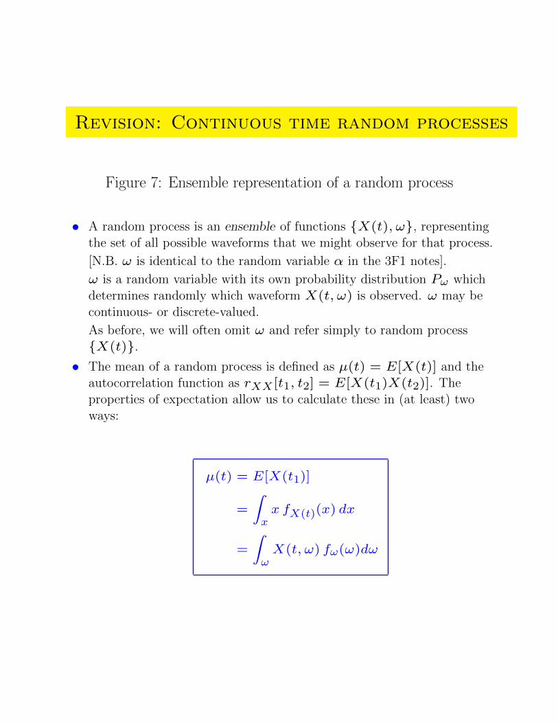
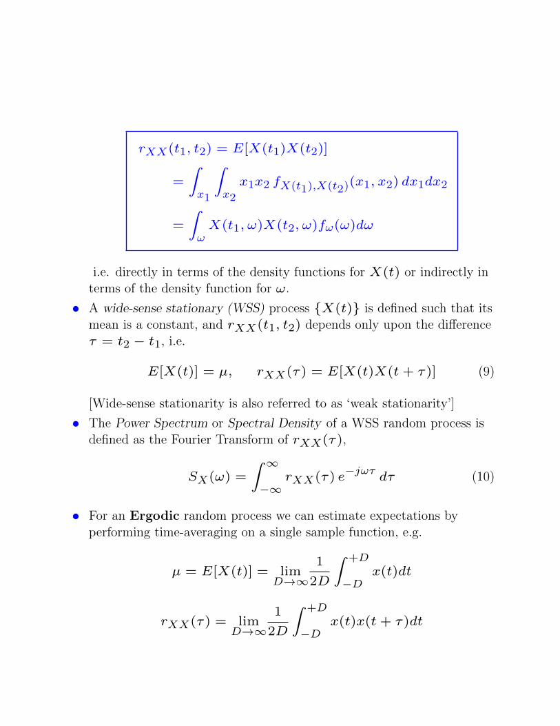
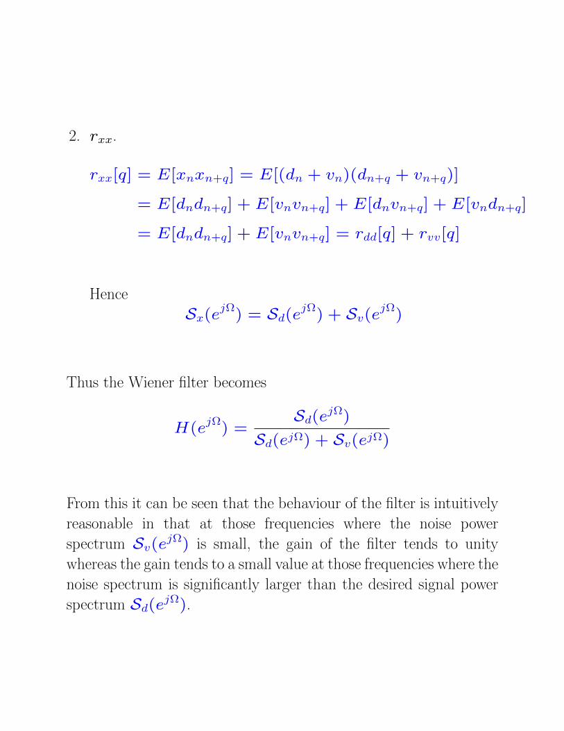
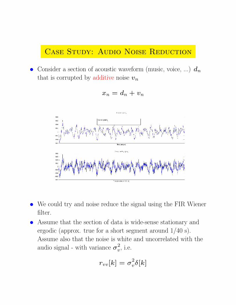
bull The Wiener filter in this case needs (see eq (23))
rxx[k] Autocorrelation of noisy signal
rxd[k] = rdd[k] Autocorrelation of desired signal
[since noise uncorrelated with signal as in eq (19)]
bull Since signal is assumed ergodic we can estimate these
quantities
rxx[k] asymp1
N
Nminus1sumn=0
xnxn+k
rdd[k] = rxx[k]minus rvv[k] =
rxx[k] k 6= 0
rxx[0]minus σ2v k = 0
[Note have to be careful that rdd[k] is still a valid
autocorrelation sequence since rxx is just an estimate]
bull Choose the filter length P form the autocorrelation matrix and
cross-correlation vector and solve in eg Matlab
h = Rxminus1
rxd
bull The output looks like this with P = 350
bull The theoretical mean-squared error is calculated as
Jmin = rdd[0]minus rTxdh
bull We can compute this for various filter lengths and in this
artificial scenario we can compare the theoretical error
performance with the actual mean-squared error since we have
access to the true dn itself
Jtrue =1
N
Nminus1sumn=0
(dn minus dn)2
Not necessarily equal to the theoretical value since we estimated
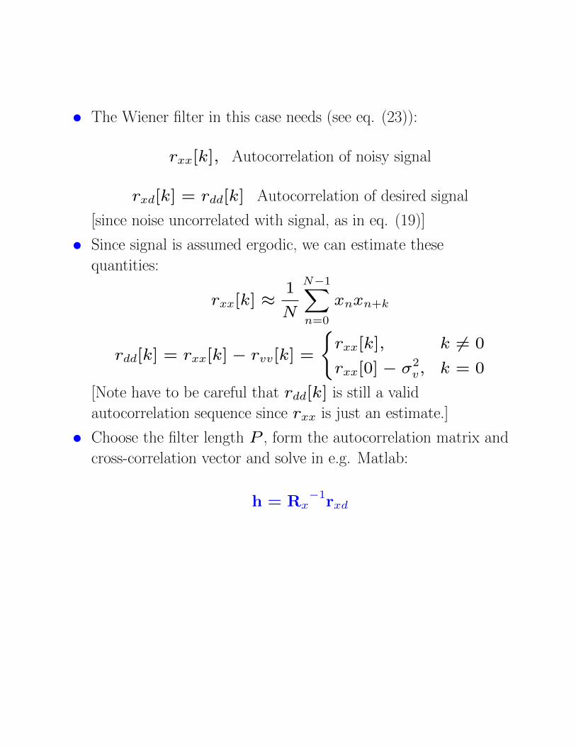
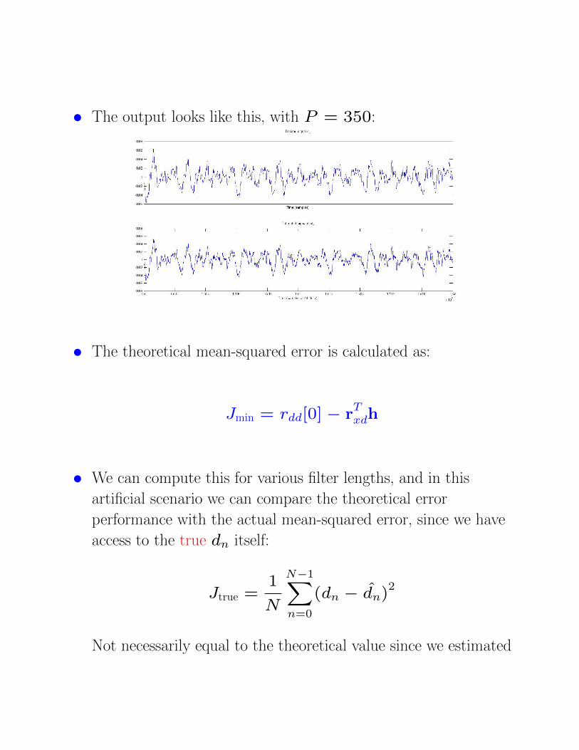
the autocorrelation functions from finite pieces of data and
assumed stationarity of the processes
Example AR process
Now take as a numerical example the exact same setup but we
specify
Example Noise cancellation
Matched Filtering
bull The Wiener filter shows how to extract a random signal from a
random noise environment
bull How about the (apparently) simpler task of detecting a known
deterministic signal sn n = 0 N minus 1 buried in random
noise vn
xn = sn + vn
bull The technical method for doing this is known as the matched
filter
bull It finds extensive application in detection of pulses in
communications data radar and sonar data
bull To formulate the problem first lsquovectorisersquo the equation
x = s + v
s = [s0 s1 sNminus1]T x = [x0 x1 xNminus1]
T
bull Once again we will design an optimal FIR filter for performing
the detection task Suppose the filter has coefficients hm for
m = 0 1 N minus 1 then the output of the filter at time
N minus 1 is
yNminus1 =
Nminus1summ=0
hmxNminus1minusm = hTx = h
T(s + v) = h
Ts+h
Tv
where x = [xNminus1 xNminus2 x0]T etc (lsquotime-reversedrsquo
vector)
bull This time instead of minimising the mean-squared error as in
the Wiener Filter we attempt to maximise the signal-to-noise
ratio (SNR) at the output of the filter hence giving best
possible chance of detecting the signal sn
bull Define output SNR as
E[|hT s|2]E[|hT v|2]
=|hT s|2
E[|hT v|2]
[since numerator is not a random quantity]
Signal output energy
bull The signal component at the output is hT s with energy
|hT s|2 = hTssTh
bull To analyse this consider the matrix M = ssT What are its
eigenvectorseigenvalues
bull Recall the definition of eigenvectors (e) and eigenvalues (λ)
Me = λe
bull Try e = s
Ms = ssTs = (s
Ts)s
Hence the unit length vector e0 = s|s| is an eigenvector and
λ = (sT s) is the corresponding eigenvalue
bull Now consider any vector eprime which is orthogonal to e0 (ie
sTeprime = 0)
Meprime= ss
Teprime= 0
Hence eprime is also an eigenvector but with eigenvalue λprime = 0
Since we can construct a set of N minus 1 orthonormal (unit length
and orthogonal to each other) vectors which are orthogonal to
s call these e1 e2 eNminus1 we have now discovered all N
eigenvectorseigenvalues of M
bull Since the N eigenvectors form an orthonormal basis we may
represent any filter coefficient vector h as a linear combination
of these
h = αe0 + βe1 + γe2 + + eNminus1
bull Now consider the signal output energy again
hTssTh = h
TssT(αe0 + βe1 + γe2 + + eNminus1)
= hT(αs
Ts)e0 because Me0 = (s
Ts)e0
= (αe0 + βe1 + γe2 + + eNminus1)T(αs
Ts)e0
= α2sTs
since eTi ej = δ[iminus j]
Noise output energy
bull Now consider the expected noise output energy which may be
simplified as follows
E[|hT v|2] = E[hTvv
Th] = h
TE[vv
T]h
bull We will here consider the case where the noise is white with
variance σ2v Then for any time indexes i = 0 N minus 1 and
j = 0 N minus 1
E[vivj] =
σ2v i = j
0 i 6= j
and hence
E[vvT] = σ
2vI
where I is the N timesN identity matrix
[diagonal elements correspond to i = j terms and off-diagonal
to i 6= j terms]
bull So we have finally the expression for the noise output energy
E[|hT v|2] = hTσ
2vIh = σ
2vh
Th
and once again we can expand h in terms of the eigenvectors of
M
σ2vh
Th = σ
2v(α
2+ β
2+ γ
2+ )
again since eTi ej = δ[iminus j]
SNR maximisation
bull The SNR may now be expressed as
|hT s|2
E[|hT v|2]=
α2sT s
σ2v(α
2 + β2 + γ2 + )
bull Clearly scaling h by some factor ρ will not change the SNR
since numerator and denominator will both then scale by ρ2
So we can arbitrarily fix |h| = 1 (any other value except zero
would do but 1 is a convenient choice) and then maximise
bull With |h| = 1 we have (α2 + β2 + γ2 + ) = 1 and the
SNR becomes just equal to α2sT s(σ2v times 1)
bull The largest possible value of α given that |h| = 1 corresponds
to α = 1 which implies then that β = γ = = 0 and
finally we have the solution as
hopt
= 1times e0 =s
|s| since e0 =
s
|s|
ie the optimal filter coefficients are just the (normalised)
time-reversed signal
bull The SNR at the optimal filter setting is given by
SNRopt
=sT s
σ2v
and clearly the performance depends (as expected) very much
on the energy of the signal s and the noise v
Practical Implementation of the matched filter
bull We chose a batch of data of same length as the signal s and
optimised a filter h of the same length
bull In practice we would now run this filter over a much longer
length of data x which contains s at some unknown position
and find the time at which maximum energy occurs This is the
point at which s can be detected and optimal thresholds can be
devised to make the decision on whether a detection of s should
be declared at that time
bull Example (like a simple square pulse radar detection problem)
sn = Rectangle pulse =
1 n = 0 1 T minus 1
0 otherwise
bull Optimal filter is the (normalised) time reversed version of sn
hoptn =
1radicT n = 0 1 T minus 1
0 otherwise
bull SNR achievable at detection point
SNRopt
=sT s
σ2v
=T
σ2v
Compare with best SNR attainable before matched filtering
SNR =Max signal value2
Average noise energy=
1
σ2v
ie a factor of T improvemment which could be substantial for
long pulses T gtgt 1
bull See below for example inputs and outputs
bull See below for a different case where the signal is a saw-tooth
pulse
sn = Sawtooth pulse =
n+ 1 n = 0 1 T minus 1
0 otherwise
Section 3 Model-based signal processing
In this section some commonly used signal models for random
processes are described and methods for their parameter estimation
are presented
bull If the physical process which generated a set of data is known or
can be well approximated then a parametric model can be
constructed
bull Careful estimation of the parameters in the model can lead to
very accurate estimates of quantities such as power spectrum
bull We will consider the autoregressive moving-average (ARMA)
class of models in which a LTI system (digital filter) is driven by
a white noise input sequence
bull If a random process Xn can be modelled as white noise
exciting a filter with frequency response H(ejΩ) then the
spectral density of the process is
SX(ejΩ
) = σ2w |H(e
jΩ)|2
where σ2w is the variance of the white noise process In its
general form this is known as the innovations representation of
a random process It can be shown that any regular (ie not
predictable with zero error) stationary random process can be
expressed in this form
bull We will study models in which the frequency response H(ejΩ)
is that of an IIR digital filter in particular the all-pole case
(known as an AR model)
bull Parametric models need to be chosen carefully - an
inappropriate model for the data can give misleading results
bull We will also study parameter estimation techniques for signal
models
ARMA Models
A quite general representation of a stationary random process is the
autoregressive moving-average (ARMA) model
bull The ARMA(PQ) model difference equation representation is
xn = minusPsump=1
ap xnminusp +
Qsumq=0
bq wnminusq (24)
where
ap are the AR parameters
bq are the MA parameters
and Wn is a zero-mean stationary white noise process with
variance σ2w Typically b0 = 1 as otherwise the model is
redundantly parameterised (any arbitrary value of b0 could be
equivalently modelled by changing the value of σv)
bull Clearly the ARMA model is a pole-zero IIR filter-based model
with transfer function
H(z) =B(z)
A(z)
where
A(z) = 1 +Psump=1
apzminusp B(z) =
Qsumq=0
bqzminusq
bull Unless otherwise stated we will always assume that the filter is
stable ie the poles (solutions of A(z) = 0) all lie within the
unit circle (we say in this case that A(z) is minimum phase)
Otherwise the autocorrelation function is undefined and the
process is technically non-stationary
bull Hence the power spectrum of the ARMA process is
SX(ejωT
) = σ2w
|B(ejωT )|2
|A(ejωT )|2
bull Note that as for standard digital filters A(z) and B(z) may
be factorised into the poles dq and zeros cq of the system In
which case the power spectrum can be given a geometric
interpretation (see eg 3F3 laboratory)
|H(ejΩ
)| = G
prodQq=1 Distance from ejΩ to cqprodPp=1 Distance from ejΩ to dp
bull The ARMA model and in particular its special case the AR
model (Q = 0) are used extensively in applications such as
speech and audio processing time series analysis econometrics
computer vision (tracking)
The ARMA model is quite a flexible and general way to model a
stationary random process
bull The poles model well the peaks in the spectrum (sharper peaks
implies poles closer to the unit circle)
bull The zeros model troughs or nulls in the power spectrum
bull Highly complex power spectra can be approximated well by
large model orders P and Q
AR models
The AR model despite being less general than the ARMA model
is used in practice far more often owing to the simplicity of its
mathematics and the efficient ways in which its parameters may be
estimated from data Hence we focus on AR models from here on
ARMA model parameter estimation in contrast requires the solution
of troublesome nonlinear equations and is prone to local maxima in
the parameter search space It should be noted that an AR model
of sufficiently high order P can approximate any particular ARMA
model
The AR model is obtained in the all-pole filter case of the ARMA
model for which Q = 0 Hence the model equations are
xn = minusPsump=1
ap xnminusp + wn (25)
Autocorrelation function for AR Models
The autocorrelation function rXX[r] for the AR process is
rXX[r] = E[xnxn+r]
Substituting for xn+r from Eq (25) gives
rXX[r] = E
xnminus
Psump=1
ap xn+rminusp + wn+r
= minusPsump=1
apE[xnxn+rminusp] + E[xnwn+r]
= minusPsump=1
ap rXX[r minus p] + rXW [r]
Note that the auto-correlation and cross-correlation satisfy the same
AR system difference equation as xn and wn (Eq 25)
Now let the impulse response of the system H(z) = 1A(z) be hn
then
xn =infinsum
m=minusinfinhmwnminusm
Then from the linear system results of Eq (3)
rXW [k] = rWX[minusk]
= hminusk lowast rWW [minusk] =infinsum
m=minusinfinhminusm rWW [mminus k]
[ Note that we have used the results that rXY [k] = rY X[minusk] and
rXX[k] = rXX[minusk] for stationary processes]
Wn is however a zero-mean white noise process whose
autocorrelation function is
rWW [m] = σ2Wδ[m]
and hence
rXW [k] = σ2Whminusk
Substituting this expression for rXW [k] into equation gives the
so-called Yule-Walker Equations for an AR process
rXX[r] = minusPsump=1
ap rXX[r minus p] + σ2Whminusr (26)
Since the AR system is causal all terms hk are zero for k lt 0
Now consider inputing the unit impulse δ[k] in to the AR difference
equation It is then clear that
h0 = minusPsumi=1
ai(hminusi = 0) + 1 = 1
Hence the Yule-Walker equations simplify to
rXX[r] +
Psump=1
ap rXX[r minus p] =
σ2W r = 0
0 Otherwise(27)
or in matrix formrXX[0] rXX[minus1] rXX[minusP ]
rXX[1] rXX[0] rXX[1minus P ]
rXX[P ] rXX[P minus 1] rXX[0]
1
a1
aP
=
σ2W
0
0
This may be conveniently partitioned as followsrXX[0] rXX[minus1] rXX[minusP ]
rXX[1] rXX[0] rXX[1minus P ]
rXX[P ] rXX[P minus 1] rXX[0]
1
a1
aP
=
σ2W
0
0
Taking the bottom P elements of the right and left hand sidesrXX[0] rXX[minus1] rXX[1minus P ]
rXX[1] rXX[0] rXX[2minus P ]
rXX[P minus 1] rXX[P minus 2] rXX[0]
a1
a2
aP
= minus
rXX[1]
rXX[2]
rXX[P ]
or
Ra = minusr (28)
and
σ2W =
[rXX[0] rXX[minus1] rXX[minusP ]
]
1
a1
a2
aP
This gives a relationship between the AR coefficients the
autocorrelation function and the noise variance terms If we can
form an estimate of the autocorrelation function using the observed
data then (28) above may be used to solve for the AR coefficients as
a = minusRminus1r (29)
Example AR coefficient estimation
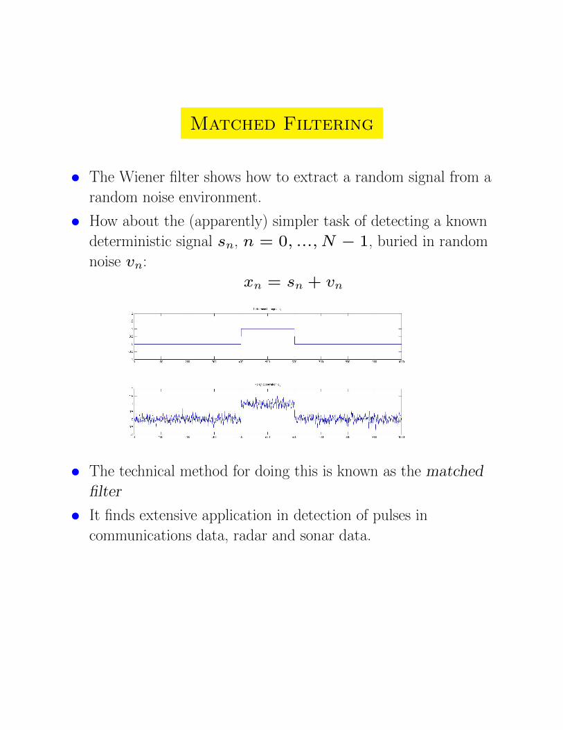
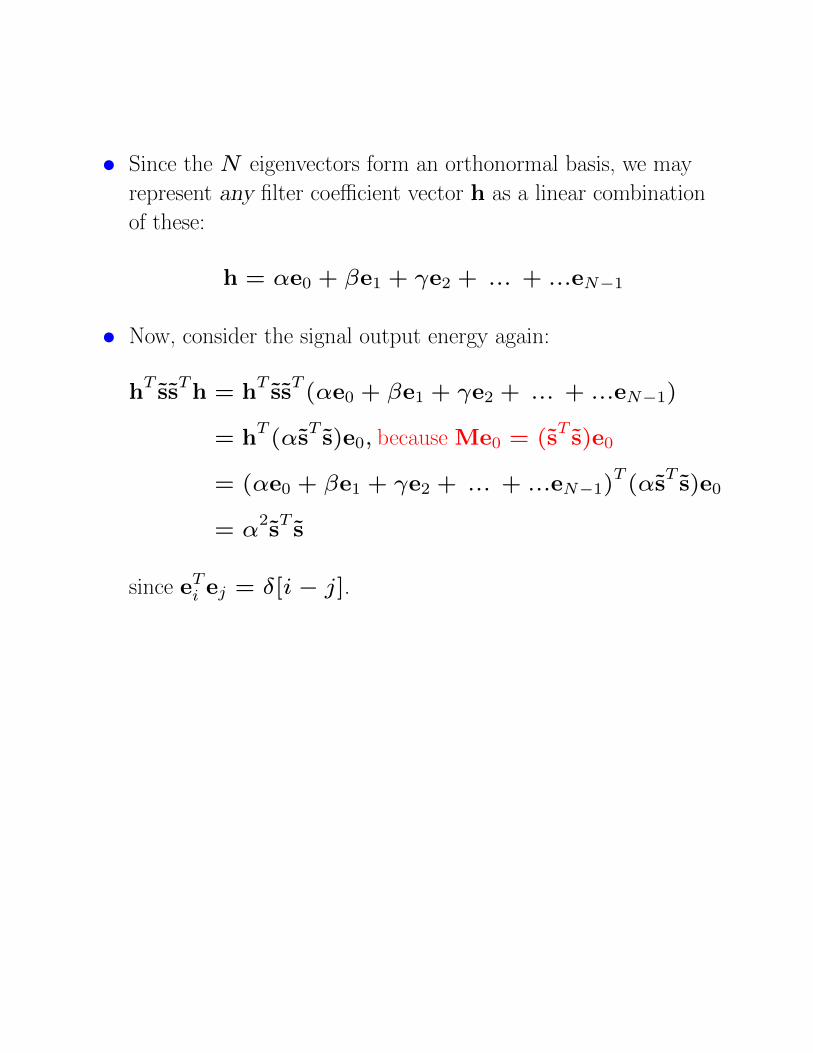
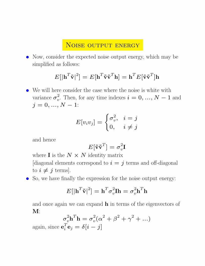
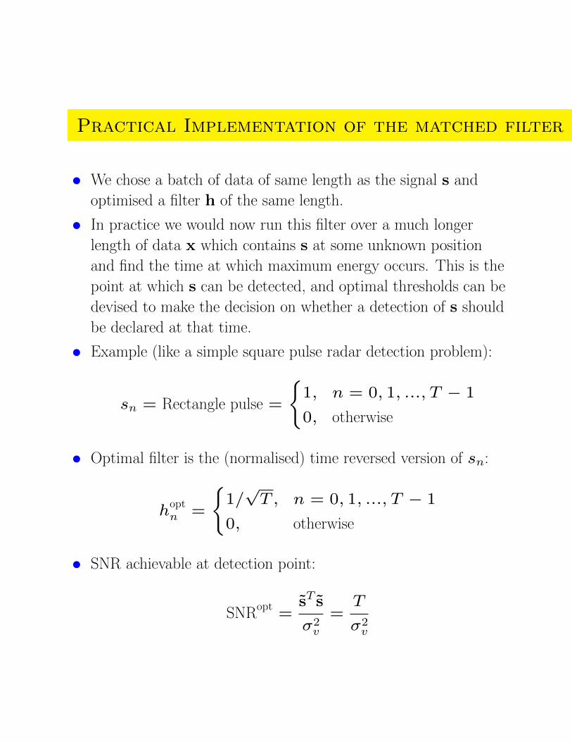
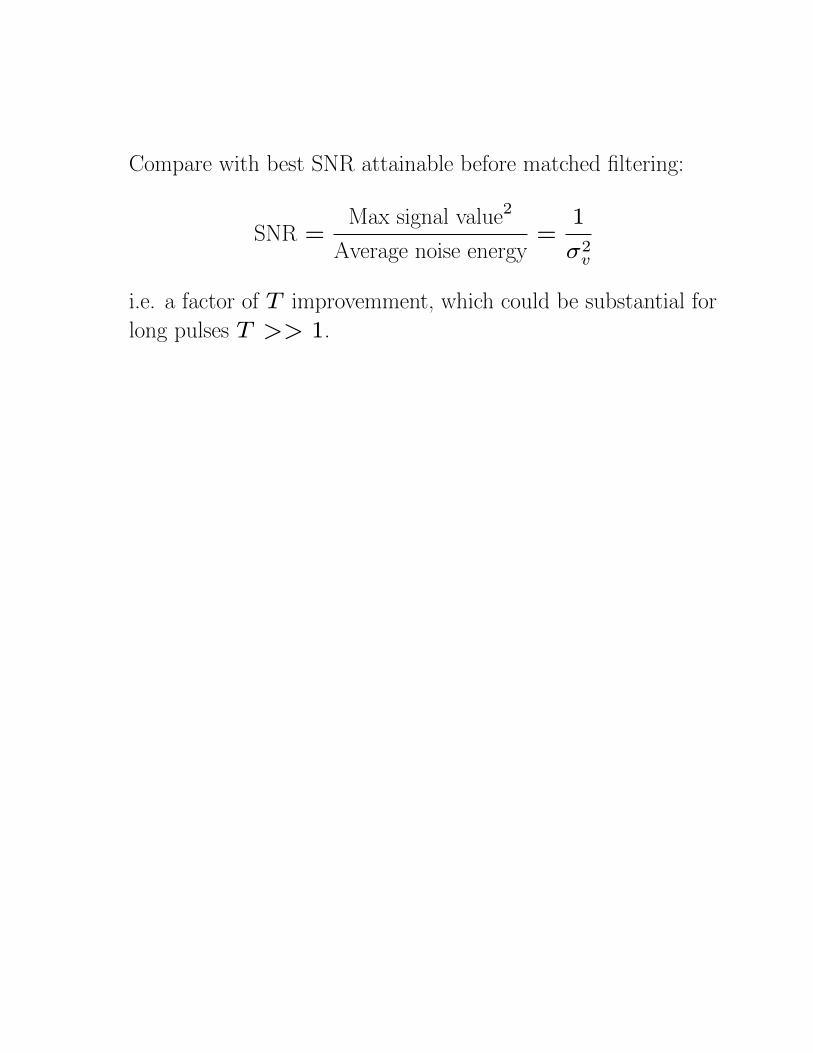
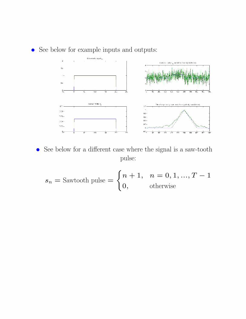
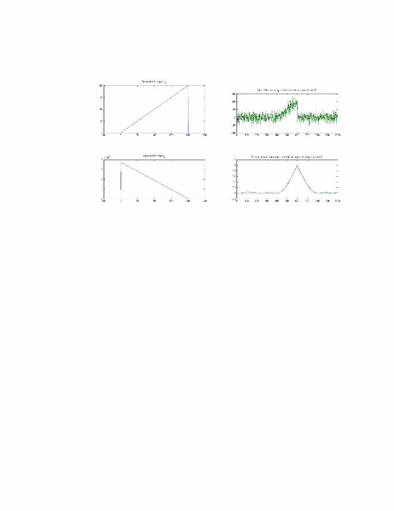
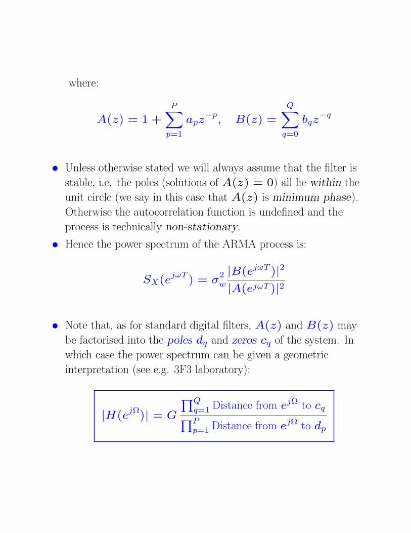
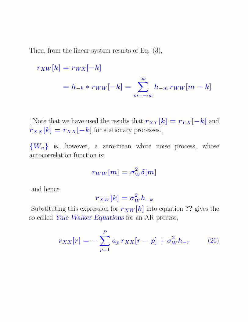
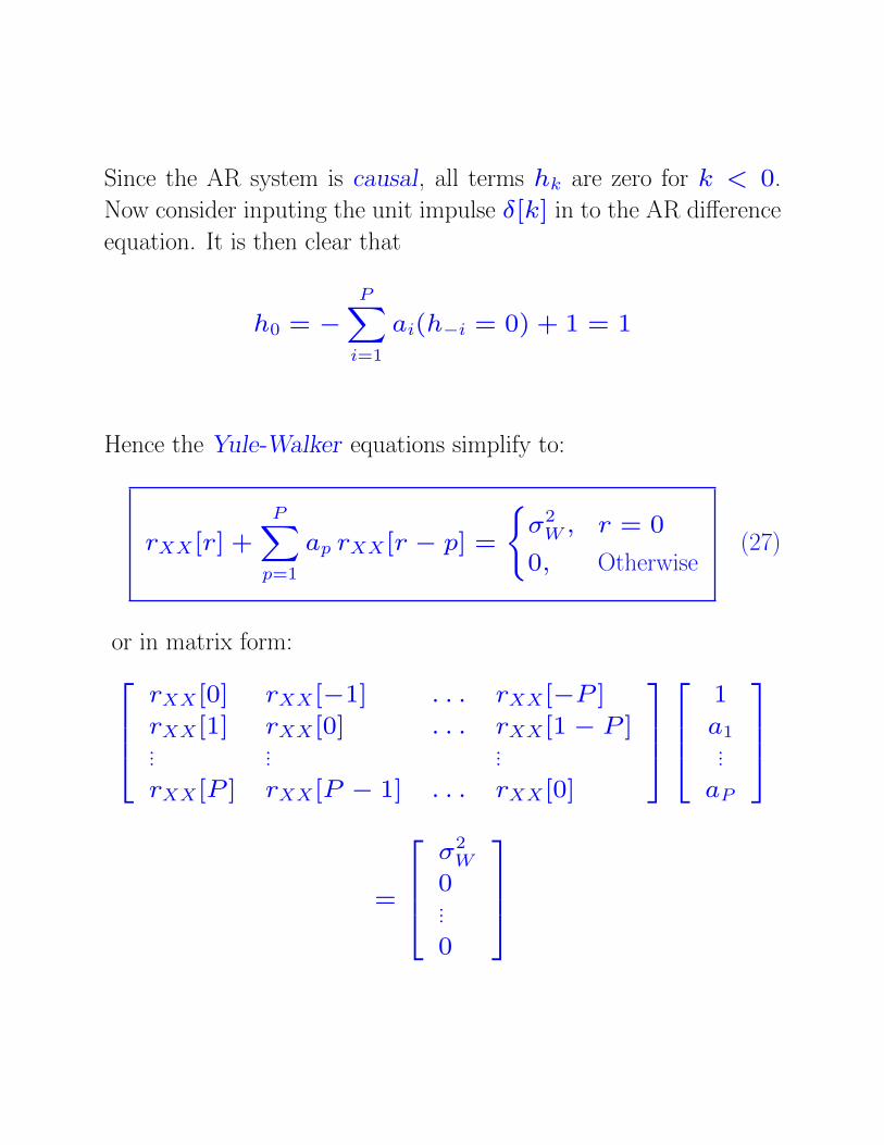
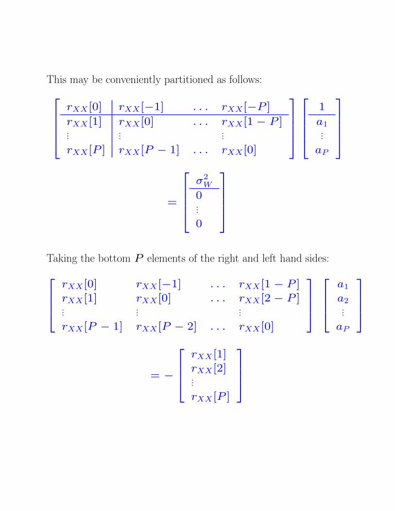
Example AR coefficient estimation