1

UNIT - III

RANDOM PROCESSES

Introduction

In chapter 1, we discussed about random variables. Random variable is a function of the

possible outcomes of a experiment. But, it does not include the concept of time. In the

real situations, we come across so many time varying functions which are random in

nature. In electrical and electronics engineering, we studied about signals.

Generally, signals are classified into two types.

(i) Deterministic

(ii) Random

Here both deterministic and random signals are functions of time. Hence it is

possible for us to determine the value of a signal at any given time. But this is not

possible in the case of a random signal, since uncertainty of some element is always

associated with it. The probability model used for characterizing a random signal is called

a random process or stochastic process.

RANDOM PROCESS CONCEPT

A random process is a collection (ensemble) of real variable {X(s, t)} that are functions

of a real variable t where s S, S is the sample space and

t T. (T is an index set).

REMARK

i) If t is fixed, then {X(s, t)} is a random variable.

ii) If S and t are fixed {X(s, t)} is a number.

iii) If S is fixed, {X(s, t)} is a signal time function.

NOTATION

Here after we denote the random process {X(s, t)} by {X(t)} where the index set T is assumed to

be continuous process is denoted by {X(n)} or {Xn}.

A comparison between random variable and random process

Random Variable Random Process

A function of the possible outcomes of

an experiment is X(s)

A function of the possible outcomes of

an experiment and also time i.e, X(s, t)

Outcome is mapped into a number x. Outcomes are mapped into wave from

which is a fun of time 't'.

CLASSIFICATION OF RANDOM PROCESSES

We can classify the random process according to the characteristics of time t and the

random variable X = X(t) t & x have values in the ranges

–< t < and –< x <.

CONTINUOUS RANDOM PROCESS

If 'S' is continuous and t takes any value, then X(t) is a continuous random variable.

Example

Let X(t) = Maximum temperature of a particular place in (0, t). Here 'S' is a continuous

set and t 0 (takes all values), {X(t)} is a continuous random process.

DISCRETE RANDOM PROCESS

If 'S' assumes only discrete values and t is continuous then we call such random process {X(t) as Discrete Random Process.

Example

Let X(t) be the number of telephone calls received in the interval (0, t).

Here, S = {1, 2, 3, …}

T = {t, t 0}

{X(t)} is a discrete random process.

CONTINUOUS RANDOM SEQUENCE If 'S' is a continuous but time 't' takes only discrete is called discrete random sequence.

Example: Let Xn denote the outcome of the nth

toss of a fair die.

Here S = {1, 2, 3, 4, 5, 6} T = {1, 2, 3, …}

(Xn, n = 1, 2, 3, …} is a discrete random sequence.

Random Process is a function of

Random Variables Time t

Discrete Continuous Discrete Continuous

CLASSIFICATION OF RANDOM PROCESSES BASED ON ITS SAMPLE

FUNCTIONS

Non-Deterministic Process

A Process is called non-deterministic process if the future values of any sample function

cannot be predicted exactly from observed values.

Deterministic Process

A process is called deterministic if future value of any sample function can be predicted

from past values.

STATIONARY PROCESS

A random process is said to be stationary if its mean, variance, moments etc are constant.

Other processes are called non stationary.

1. 1st Order Distribution Function of {X(t)}

For a specific t, X(t) is a random variable as it was observed earlier.

F(x, t) = P{X(t) x} is called the first order distribution of the process {X(t)}.

1st

Order Density Function of {X(t)}

f x, t

Fx, t is called the first order density of {X, t}

x

2nd

Order distribution function of {X(t)}

Fx1, x2; t1, t2 PX t1 x1; X t2 x2 is the point distribution of the random

variables X(t1) and X(t2) and is called the second order distribution of the process {X(t)}.

2nd

order density function of {X(T)}

f x ,x ; t ,t Fx1, x2; t1, t2 is called the second order density of {X(t)}.

1 2 1 2 x, x2

First - Order Stationary Process

Definition

A random process is called stationary to order, one or first order stationary if its 1st

order

density function does not change with a shift in time origin. In other words,

fX x1, t1 fX x1, t1 Cmust be true for any t1 and any real number C if {X(t1)} is to

be a first order stationary process.

Example :1

Show that a first order stationary process has a constant mean.

Solution

Let us consider a random process {X(t1)} at two different times t1 and t2.

2

E X t1

xf x, t1 dx

[f(x,t1) is the density form of the random process X(t1)]

E X t2 xf x, t2 dx

Let t2 = t1 + C [f(x,t2) is the density form of the random process X(t2)]

E X t2 xf x, t1 Cdx xf x, t1 dx

= E X t1 Thus E X t2 E X t1

Mean process {X(t1)} = mean of the random process {X(t2)}. Definition 2:

If the process is first order stationary, then

Mean = E(X(t)] = constant

Second Order Stationary Process

A random process is said to be second order stationary, if the second order density

function stationary.

f x1, x2; t1, t2 f x1, x2; t1 C, t2 Cx1, x2 and C. 2 2 E X1 ,E X2 ,E X1, X2 denote change with time, where

X = X(t1); X2 = X(t2).

Strongly Stationary Process

A random process is called a strongly stationary process or Strict Sense Stationary

Process (SSS Process) if all its finite dimensional distribution are invariance under translation of

time 't'.

fX(x1, x2; t1, t2) = fX(x1, x2; t1+C, t2+C)

fX(x1, x2, x3; t1, t2, t3) = fX(x1, x2, x3; t1+C, t2+C, t3+C) In general

fX(x1, x2..xn; t1, t2…tn) = fX(x1, x2..xn; t1+C, t2+C..tn+C) for any t1 and any real number C.

Jointly - Stationary in the Strict Sense

{X(t)} and Y{(t)} are said to be jointly stationary in the strict sense, if the joint

distribution of X(t) and Y(t) are invariant under translation of time.

Definition Mean:

X t E X t1 , t

X t is also called mean function or ensemble average of the random process.

Auto Correlation of a Random Process

2

Let X(t1) and X(t2) be the two given numbers of the random process {X(t)}. The auto

correlation is

R XX t1, t2 EX t1 xX t2 Mean Square Value

Putting t1 = t2 = t in (1), we get

RXX (t,t) = E[X(t) X(t)]

R XX t, t E X t is the mean square value of the random process.

Auto Covariance of A Random Process

CXX t1, t2 EX t1 E X t1 X t2 E X t2

= R XX t1, t2 E X t1 E X t2 Correlation Coefficient

The correlation coefficient of the random process {X(t)} is defined as

t ,t CXX t1,t2 XX 1 2

Var X t1 xVar X t2 Where CXX (t1, t2) denotes the auto covariance.

CROSS CORRELATION

The cross correlation of the two random process {X(t)} and {Y(t)} is defined by

RXY (t1, t2) = E[X(t1) Y (t2)]

WIDE - SENSE STATIONARY (WSS)

A random process {X(t)} is called a weakly stationary process or covariance stationary

process or wide-sense stationary process if i) E{X(t)} = Constant

ii) E[X(t) X(t+] = RXX() depend only on when = t2 - t1.

REMARKS :

SSS Process of order two is a WSS Process and not conversely.

EVOLUTIONARY PROCESS

A random process that is not stationary in any sense is called as evolutionary process.

SOLVED PROBLEMS ON WIDE SENSE STATIONARY PROCESS

Example:1

Given an example of stationary random process and justify your claim.

Solution:

Let us consider a random process X(t) = A as (wt + ) where A & are custom and '' is

uniformlydistribution random Variable in the interval

(0, 2).

Since '' is uniformly distributed in (0, 2), we have

1 n 1

2

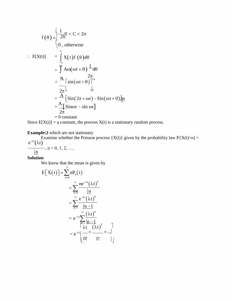
1 ,0 C 2

f 20 , otherwise

E[X(t)] =

=

X tf d

At 1

d

0 2

= A

sin t 2

2 0

= A

Sin 2 t Sin t 0 2

= A Sint sin t

2= 0 constant

Since E[X(t)] = a constant, the process X(t) is a stationary random process.

Example:2 which are not stationary Examine whether the Poisson process {X(t)} given by the probability law P{X(t)=n] =

et t

, n = 0, 1, 2, ….

Solution

We know that the mean is given by

E X t nPn t n0

= n0

= n

net t

n

et t

n

= ett

n

n1 n 1 t t

2

= et ...

0! 1!

n

n

2T

t t 2

= t et 1 ... 1 2

= t etet

= t , depends on t

Hence Poisson process is not a stationary process.

ERGODIC RANDOM PROCESS

Time Average

The time average of a random process {X(t)} is defined as

1 T

XT Xtdt T

Ensemble Average

The ensemble average of a random process {X(t)} is the expected value of the random

variable X at time t

Ensemble Average = E[X(t)]

Ergodic Random Process

{X(t)} is said to be mean Ergodic

If lim X T T

T

lim 1

Xtdt T 2T

T

Mean Ergodic Theorem

Let {X(t)} be a random process with constant mean and let XT

Then {X(t)} is mean ergodic if

be its time average.

lim Var X T 0 T

Correlation Ergodic Process

The stationary process {X(t)} is said to be correlation ergodic if the process {Y(t)} is

mean ergodic where

Y(t) = X(t) X(t+)

TUTORIAL QUESTIONS

1.. The t.p.m of a Marko cain with three states 0,1,2 is P=

and the initial state distribution is

Find (i)P[X2=3] ii)P[X3=2, X2=3, X1=3, X0=2] 2. Three boys A, B, C are throwing a ball each other. A always throws the ball to B and B

always throws the ball to C, but C is just as likely to throw the ball to B as to A. S.T. the process

is Markovian. Find the transition matrix and classify the states

3. A housewife buys 3 kinds of cereals A, B, C. She never buys the same cereal in successive

weeks. If she buys cereal A, the next week she buys cereal B. However if she buys P or C the

next week she is 3 times as likely to buy A as the other cereal. How often she buys each of the

cereals?

4. A man either drives a car or catches a train to go to office each day. He never goes 2 days in a row by train but if he drives one day, then the next day he is just as likely to drive again as he is to travel by train. Now suppose that on the first day of week, the man tossed a fair die and drove

to work if a 6 appeared. Find 1) the probability that he takes a train on the 3rd

day. 2). The probability that he drives to work in the long run.

WORKED OUT EXAMPLES

Example:1.Let Xn denote the outcome of the nth

toss of a fair die.

Here S = {1, 2, 3, 4, 5, 6}

T = {1, 2, 3, …}

(Xn, n = 1, 2, 3, …} is a discrete random sequence.

Example:2 Given an example of stationary random process and justify your claim.

Solution:

Let us consider a random process X(t) = A as (wt + ) where A & are custom and '' is

uniformly distribution random Variable in the interval

(0, 2).

Since '' is uniformly distributed in (0, 2), we have

1 ,0 C 2

f 20 , otherwise

E[X(t)] =

X tf d

n

1 n 1

2

= At 1

d

0 2

= A

sin t 2

2 0

= A

Sin 2 t Sin t 0 2

= A Sint sin t

2= 0 constant

Since E[X(t)] = a constant, the process X(t) is a stationary random process.

Example:3.which are not stationary .Examine whether the Poisson process {X(t)} given by the et t

probability law P{X(t)=n] = , n = 0, 1, 2, ….

Solution

We know that the mean is given by

E X t nPn t n0

= n0

= n

net t

n

et t

n

= ett

n

n1 n 1 t t

2

= et ...

0! 1! 2 t t= t et 1 ... 1 2

= t etet

= t , depends on t

Hence Poisson process is not a stationary process.

n

60

CORRELATION AND SPECTRAL DENSITY

Introduction

The power spectrum of a time series x(t) describes how the variance of the data x(t) is

distributed over the frequency components into which x(t) may be decomposed. This

distribution of the variance may be described either by a measure or by a statistical

cumulative distribution function S(f) = the power contributed by frequencies from 0 upto

f. Given a band of frequencies [a, b) the amount of variance contributed to x(t) by

frequencies lying within the interval [a,b) is given by S(b) - S(a). Then S is called the

spectral distribution function of x.

The spectral density at a frequency f gives the rate of variance contributed by

frequencies in the immediate neighbourhood of f to the variance of x per unit frequency.

Auto Correlation of a Random Process

Let X(t1) and X(t2) be the two given random variables. Then auto correlation is

RXX (t1, t2) = E[X(t1) X(t2)]

Mean Square Value

Putting t1 = t2 = t in (1) RXX (t, t) = E[X(t) X(t)]

RXX (t, t) = E[X2(t)]

Which is called the mean square value of the random process.

Auto Correlation Function

Definition: Auto Correlation Function of the random process {X(t)} is

RXX = () = E{(t) X(t+)}

Note: RXX () = R() = RX ()

PROPERTY: 1

The mean square value of the Random process may be obtained from the auto correlation

function.

RXX(), by putting = 0. is known as Average power of the random process {X(t)}.

PROPERTY: 2

RXX() is an even function of .

RXX () = RXX (-)

PROPERTY: 3

If the process X(t) contains a periodic component of the same period.

PROPERTY: 4

If a random process {X(t)} has no periodic components, and

E[X(t)] = X then

2

2

2

lim R XX X (or)X |T|

lim R XX |T|

i.e., when , the auto correlation function represents the square of the mean of the random

process.

PROPERTY: 5

The auto correlation function of a random process cannot have an arbitrary shape.

SOLVED PROBLEMS ON AUTO CORRELATION

Example : 1

Check whether the following function are valid auto correlation function (i) 5 sin n (ii)

1

1 92

Solution:

(i) Given RXX() = 5 Sin n

RXX (–) = 5 Sin n(–) = –5 Sin n

RXX() RXX(–), the given function is not an auto correlation function.

1 (ii) Given RXX () =

1 92

1 RXX (–) =

1 92

R XX

The given function is an auto correlation function.

Example : 2

Find the mean and variance of a stationary random process whose auto correlation

function is given by

R XX 18 2

6

Solution

Given R XX 18 2

6 X

2 lim R

| | XX

= lim 18

2

| |

= 18 lim

6 2

2

| | 6 2

2

1

= 18 2

6

= 18 + 0

= 18

X = 18

E X t = 18

Var {X(t)} = E[X2(t)] - {E[X(t)]}

2

We know that

E X2 t = RXX(0)

2 55 = 18

6 0 3 1

= 3

Example : 3

Express the autocorrelation function of the process {X'(t)} in terms of the auto correlation

function of process {X(t)}

Solution

Consider, RXX'(t1, t2) = E{X(t1)X'(t2)}

= E X t lim

X t2 h X t2 1

n0

h

X t1 X t2 h X t1 X t2

= lim E

h0 h

RXX t1,t2 h RX t1,t2 = lim

RXX' (t1, t2) =

Similarly RXX' (t1, t2) =

h0 h

R t , t

t XX 1 2

R ' t, t

t XX 2

(1)

RX'X (t1, t2) =

t, t2

R XX t1, t2 by (1)

Auto Covariance

The auto covariance of the process {X(t)} denoted by CXX(t1, t2) or C(t1, t2) is defined as

R XX 0R YY 0

CXX t1, t2 EX t1 E X t1 X t2 E X t2 CORRELATION COEFFICIENT

XX t1,t2 CXX t1,t2

Where CXX(t1, t2) denotes the auto covariance.

CROSS CORRELATION

Cross correlation between the two random process {X(t)} and {Y(t)} is defined as

RXY (t1, t2) = E[X(t1) Y(t2)] where X(t1) Y(t2) are random variables.

CROSS COVARIANCE

Let {X(t)} and {Y(t)} be any two random process. Then the cross covariance is defined as

CXY t1, t2 EX t1 E Y t1 X t2 E Y t2 The relation between Mean Cross Correlation and cross covariance is as follows:

CXY t1,t2 Definition

R XY t1, t2 E X t1 E Y t2

Two random process {X(t)} and {Y(t)} are said to be uncorrelated if

CXY t1,t2 0, t1,t2

Hence from the above remark we have,

RXY (t1, t2) = E[X(t1) Y(t2)]

CROSS CORRELATION COEFFICIENT

XY t1,t2 cXY t1,t2

CROSS CORRELATION AND ITS PROPERTIES

Let {X(t)} and {Y(t)} be two random. Then the cross correlation between them is also

defined as

RXY(t, t+) = E X t Y t = RXY ()

PROPERTY : 1

RXY () = RYX (–)

PROPERTY : 2

If {X(t)} and {Y(t)} are two random process then R XY , where

RXX() and RYY() are their respective auto correlation functions.

Var X t1 x Var X t2

Var X t1 Var X t2

1 2

2

PROPERTY : 3

If {X(t)} and {Y(t)} are two random process then,

R XY R XX 0 R YY 0

SOLVED PROBLEMS ON CROSS CORRELATION

Example:

Two random process {X(t)} and {Y(t)} are given by

X(t) = A cos (t+), Y(t) = A sin (t + ) where A and are constants and '' is a uniform

random variable over 0 to 2. Find the cross correlation function.

Solution

By def. we have

RXY() = RXY (t, t+)

Now, RXY (t, t+) = E[X(t). Y(t+)]

= E [A cos (t + ). A sin ( (t+) + )]

= A2E sin t cos t

Since '' is a uniformly distributed random variable we have 1

f(0) = , 0 22

Now E sin t cos t

= sin t .coswt f d2

= sin t t .cost 1

d

0 2 2

= 1

sin t cost d0

1 2

1 sin t t

= 2 0 2

sint t d

1 2 sin2t 2 sin

= d

2 0

2

2

1

1 cos2t 2 2

= sin 4 2 0

1 cos2t cos2t 0 = sin 2 0

4 2 2

1 cos2t cos2t = 2sin

4 2 2

= 1 0 2sin

41

= sin (3) 2

Substituting (3) in (1) we get

A2

R XY t, t sin 2

SPECTRAL DENSITIES (POWER SPECTRAL DENSITY)

INTRODUCTION

(i) Fourier Transformation (ii) Inverse Fourier Transform

(iii) Properties of Auto Correlation Function

(iv) Basic Trigonometric Formula

(v) Basic Integration

SPECIAL REPRESENTATION

Let x(t) be a deterministic signal. The Fourier transform of x(t) is defined as

F x t x w x t eitdt

Here X() is called "spectrum of x(t)".

Hence x(t) = Inverse Fourier Transform of X()

= 1

X eitd .

Definition

The average power P(T) of x(t) over the interval (-T, T) is given by T

PT x2 t dt

2T T

X T

2

2

1

= 1 d

(1)

Definition

2

2T

The average power PXX for the random process {X(t)} is given by T P lim

1 E X

2 t dt XX

T T

E X T

2 = lim d (2)

2

T 2T

POWER SPECTRAL DENSITY FUNCTION

Definition

If {X(t)} is a stationary process (either in the strict sense or wide sense) with auto

correlation function RXX(), then the Fourier transform of RXX() is called the power spectral

density function of {X(t)} and is denoted by SXX() or S() or SX().

SXX()= Fourier Transform of RXX ()

Thus,

= R XX

eid

SXX f R

XX

ei 2fd

WIENER KHINCHINE RELATION

SXX R

XX

eid

SXX f R

XX

ei 2fd

To find RXX() if SXX() or SXX(f) is given

R XX

1

SXX

eid [inverse Fourier transform of S XX()]

(or) R XX 1

SXX

f ei 2fd

[inverse Fourier transform of SXX(f)]

PROPERTIES OF POWER SPECTRAL DENSITY FUNCTION

Property 1:

2

2

The value of the spectral density function at zero frequency is equal to the total area

under the group of the auto correlation function. i 2fc

SXX f R XX

e d

Taking f = 0, we get

Sxx(0) = R XX d

TUTORIAL QUESTIONS

1. Find the ACF of {Y(t)} = AX(t)cos (w0+ ) where X(t) is a zero mean stationary random process with ACF A and w0 are constants and is uniformly distributed over (0, 2 ) and independent of X(t).

2. Find the ACF of the periodic time function X(t) = A sinwt

3. If X(t) is a WSS process and if Y(t) = X(t + a) – X(t – a), prove that

4. If X(t) = A sin( ), where A and are constants and is a random variable, uniformly

distributed over (- ), Find the A.C.F of {Y(t)} where Y(t) = X2(t).

5.. Let X(t) and Y(t) be defined by X(t) = Acos t + Bsin t and Y(t) = B cos t – Asin t

Where is a constant and A nd B are independent random variables both having zero mean and

varaince . Find the cross correlation of X(t) and Y(t). Are X(t) and Y(t) jointly W.S.S

processes?

6. Two random processes X(t) and Y(t) are given by X(t) = A cos ( ), Y(t) = A sin(

), where A and are constants and is uniformly distributed over (0, 2 ). Find the cross

correlation of X(t) and Y(t) and verify that .

7..If U(t) = X cos t + Y sin t and V(t) = Y cost + X sint t where X and Y are independent random

varables such that E(X) = 0 = E(Y), E[X2] = E[Y

2] = 1, show that U(t) and V(t) are not jointly

W.S.S but they are individually stationary in the wide sense.

8. Random Prosesses X(t) and Y(t) are defined by X(t) = A cos ( ), Y(t) = B cos ( )

where A, B and are constants and is uniformly distributed over (0, 2 ). Find the cross

correlation and show that X(t) and Y(t) are jointly W.S.S

WORKEDOUT EXAMPLES

Example 1.Check whether the following function are valid auto correlation function (i) 5 sin n1

(ii) 1 9

2

Solution:

(i) Given RXX() = 5 Sin n

RXX (–) = 5 Sin n(–) = –5 Sin n

2

2

RXX() RXX(–), the given function is not an auto correlation function.

1 (ii) Given RXX () =

1 92

1 RXX (–) =

1 92

R XX

The given function is an auto correlation function.

Example : 2

Find the mean and variance of a stationary random process whose auto correlation

function is given by

R XX 18 2

6 Solution

Given R XX 18 2

6 X

2 lim R

| | XX

= lim 18

2

| |

= 18 lim

6 2

2

= 18

| | 6 2

2

6 = 18 + 0 = 18

X = 18

E X t = 18

Var {X(t)} = E[X2(t)] - {E[X(t)]}

2

We know that

E X2 t = RXX(0)

2 55 = 18

6 0 3 1

= 3

Example : 3

2

1

Express the autocorrelation function of the process {X'(t)} in terms of the auto correlation

function of process {X(t)}

Solution

Consider, RXX'(t1, t2) = E{X(t1)X'(t2)}

= E X t lim

X t2 h X t2 1

n0

h

X t1 X t2 h X t1 X t2

= lim E

h0 h

RXX t1,t2 h RX t1,t2 = lim

RXX' (t1, t2) =

Similarly RXX' (t1, t2) =

h0 h

R t , t

t XX 1 2

R ' t, t

t XX 2

(1)

RX'X (t1, t2) =

Example :4

t, t2

R XX t1, t2 by (1)

Two random process {X(t)} and {Y(t)} are given by

X(t) = A cos (t+), Y(t) = A sin (t + ) where A and are constants and '' is a uniform

random variable over 0 to 2. Find the cross correlation function.

Solution

By def. we have

RXY() = RXY (t, t+)

Now, RXY (t, t+) = E[X(t). Y(t+)]

= E [A cos (t + ). A sin ( (t+) + )]

= A2E sin t cos t

Since '' is a uniformly distributed random variable we have 1

f(0) = , 0 22

Now E sin t cos t

= sin t .coswt f d

2

2

= sin t t .cost

1 d

0 2 2

= 1

sin t cost d0

1 2

1 sin t t

= 2 0 2

sint t d

1 2 sin2t 2 sin

= d

2 0

2

1 cos2t 2 2

= sin 4 2 0

1 cos2t cos2t 0 = sin 2 0

4 2 2

1 cos2t cos2t = 2sin

4 2 2

= 1 0 2sin

41

= sin (3) 2

Substituting (3) in (1) we get

A2

R XY t, t sin 2

It is true that if X and Y are independent, then Cov(X, Y ) = 0. If Cov(X, Y ) = 0 then immediately

X and Y cannot be concluded that they are independent. Graphically it can be written as

X&Y independent => Cov(X,Y ) = 0

Cov(X, Y ) = 0 ≠ X&Y independent

Proof : With X=Z 2

Recognize that this last integral is (up to a scalar constant) the same integral is calculated to find E [Z],

which is 0. Therefore E [Z3] = 0. Hence Cov(X,Z) = 0 - 0 = 0. Another way to find E[Z

3] = 0 is by noticing

that x3 is an odd function, and e

-x2/2 is an even function. Hence, x3e-x2/2

is an odd function. We know that the

integral of an odd function from -∞ to ∞ is zero. Thus,

Exercise 2. Let X and Y be jointly continuous random variables with joint density

Discrete time processes and sequences A discrete-time random process x(n) is a collection, or ensemble, of discrete-time signals, xk (n)

where k is an integer. A discrete-time random process x(n) is an indexed sequence of random

variables if we look at the process at a certain ‘fixed’ time instant n (e.g., n = n0 ). The term

'discrete-time signal' is different from 'discrete-time random signal' in the present case. A discrete-

time random signal x(n) is associated with an ensemble of discrete-time signals x k(n) .

Example 1. A random process is of the form of sinusoid x(n ) = Acos( n) = A n where

A1,2,…,6 the amplitude is a random variable that assumes any integer number between

one and six, each with equal probability Pr(A=k)=1/6 (k=1, 2, …, 6). This random process consists

of an ensemble of six different discrete-time signals x k (n) , cos( nwo) ,x6(n)= 6cos(nwo),each of

which shows up with equal probability.

V+ TEAM

x1 ( n) =cos(nωo) ,x2 ( n) =2cos(nωo) ,…x6 (n ) =6cos(nωo ) ,each of which shows up with equal

probability.

The discrete-time version of a continuous-time signal x(t) is here denoted by x[n],which

corresponds to x(t) sampled at the time instant t = nT . The sampling rate is Fs =1/T in Hz, and T

is the sampling interval in seconds. The index n can be interpreted as normalized (to the sampling

rate) time. Similar to the deterministic case, it is in principle possible to reconstruct bandlimited

continuous-time stochastic process x(t) from its samples {x[n]}∞n=­∞. In the random case, the

reconstruction must be given a more precise statistical meaning, like convergence in the

mean square sense.To simplify matters, it will throughout be assumed that all processes are (

wide-sense) stationary, real valued and zero mean, i.e. E{x[n]}=0. The autocorrelation

function is defined as

The cross-correlation measures how related the two processes are. This is useful, for

example for de- termining who well one can predict a desired but unmeasurable signal y[n] from

the observed x[n]. If rxy [k] = 0 for all k, we say that x[n] and y[n] are uncorrelated. It should be

noted that the cross- correlation function is not necessarily symmetric, and it does not necessarily

have its maximum at k = 0. For example, if y[n] is a time-delayed version of x[n], y[n] = x[n − l],

then rxy [k] peaks at lag k = l. Thus, the cross-correlation can be used to estimate the time-delay

between two measurements of the same signal, perhaps taken at different spatial locations. This

can be used, for example for synchronization in a communication system.