Embed Size (px)
Citation preview
Radiative Forcing of Climate Change
Co-ordinating Lead AuthorV. Ramaswamy
Lead AuthorsO. Boucher, J. Haigh, D. Hauglustaine, J. Haywood, G. Myhre, T. Nakajima, G.Y. Shi, S. Solomon
Contributing AuthorsR. Betts, R. Charlson, C. Chuang, J.S. Daniel, A. Del Genio, R. van Dorland, J. Feichter, J. Fuglestvedt,P.M. de F. Forster, S.J. Ghan, A. Jones, J.T. Kiehl, D. Koch, C. Land, J. Lean, U. Lohmann,K. Minschwaner, J.E. Penner, D.L. Roberts, H. Rodhe, G.J. Roelofs, L.D. Rotstayn, T.L. Schneider,U. Schumann, S.E. Schwartz, M.D. Schwarzkopf, K.P. Shine, S. Smith, D.S. Stevenson, F. Stordal,I. Tegen, Y. Zhang
Review EditorsF. Joos, J. Srinivasan
6
Contents
Executive Summary 351
6.1 Radiative Forcing 3536.1.1 Definition 3536.1.2 Evolution of Knowledge on Forcing Agents 353
6.2 Forcing-Response Relationship 3536.2.1 Characteristics 3536.2.2 Strengths and Limitations of the Forcing
Concept 355
6.3 Well-Mixed Greenhouse Gases 3566.3.1 Carbon Dioxide 3566.3.2 Methane and Nitrous Oxide 3576.3.3 Halocarbons 3576.3.4 Total Well-Mixed Greenhouse Gas Forcing
Estimate 3586.3.5 Simplified Expressions 358
6.4 Stratospheric Ozone 3596.4.1 Introduction 3596.4.2 Forcing Estimates 360
6.5 Radiative Forcing By Tropospheric Ozone 3616.5.1 Introduction 3616.5.2 Estimates of Tropospheric Ozone Radiative
Forcing since Pre-Industrial Times 3626.5.2.1 Ozone radiative forcing: process
studies 3626.5.2.2 Model estimates 363
6.5.3 Future Tropospheric Ozone Forcing 364
6.6 Indirect Forcings due to Chemistry 3656.6.1 Effects of Stratospheric Ozone Changes on
Radiatively Active Species 3656.6.2 Indirect Forcings of Methane, Carbon
Monoxide and Non-Methane Hydrocarbons 3656.6.3 Indirect Forcing by NOx Emissions 3666.6.4 Stratospheric Water Vapour 366
6.7 The Direct Radiative Forcing of Tropospheric Aerosols 3676.7.1 Summary of IPCC WGI Second Assessment
Report and Areas of Development 3676.7.2 Sulphate Aerosol 3676.7.3 Fossil Fuel Black Carbon Aerosol 3696.7.4 Fossil Fuel Organic Carbon Aerosol 3706.7.5 Biomass Burning Aerosol 3726.7.6 Mineral Dust Aerosol 3726.7.7 Nitrate Aerosol 3736.7.8 Discussion of Uncertainties 374
6.8 The Indirect Radiative Forcing of Tropospheric Aerosols 3756.8.1 Introduction 3756.8.2 Indirect Radiative Forcing by Sulphate
Aerosols 3756.8.2.1 Estimates of the first indirect effect 3756.8.2.2 Estimates of the second indirect
effect and of the combined effect 3756.8.2.3 Further discussion of uncertainties 377
6.8.3 Indirect Radiative Forcing by Other Species 377
6.8.3.1 Carbonaceous aerosols 3776.8.3.2 Combination of sulphate and
carbonaceous aerosols 3786.8.3.3 Mineral dust aerosols 3786.8.3.4 Effect of gas-phase nitric acid 378
6.8.4 Indirect Methods for Estimating the Indirect Aerosol Effect 3786.8.4.1 The “missing” climate forcing 3786.8.4.2 Remote sensing of the indirect
effect of aerosols 3786.8.5 Forcing Estimates for This Report 3796.8.6 Aerosol Indirect Effect on Ice Clouds 379
6.8.6.1 Contrails and contrail-induced cloudiness 379
6.8.6.2 Impact of anthropogenic aerosols on cirrus cloud microphysics 379
6.9 Stratospheric Aerosols 379
6.10 Land-use Change (Surface Albedo Effect) 380
6.11 Solar Forcing of Climate 3806.11.1 Total Solar Irradiance 380
6.11.1.1 The observational record 3806.11.1.2 Reconstructions of past variations
of total solar irradiance 3816.11.2 Mechanisms for Amplification of Solar
Forcing 3826.11.2.1 Solar ultraviolet variation 3826.11.2.2 Cosmic rays and clouds 384
6.12 Global Warming Potentials 3856.12.1 Introduction 3856.12.2 Direct GWPs 3866.12.3 Indirect GWPs 387
6.12.3.1 Methane 3876.12.3.2 Carbon monoxide 3876.12.3.3 Halocarbons 3906.12.3.4 NOx and non-methane
hydrocarbons 391
6.13 Global Mean Radiative Forcings 3916.13.1 Estimates 3916.13.2 Limitations 396
6.14 The Geographical Distribution of the Radiative Forcings 3966.14.1 Gaseous Species 3976.14.2 Aerosol Species 3976.14.3 Other Radiative Forcing Mechanisms 399
6.15 Time Evolution of Radiative Forcings 4006.15.1 Past to Present 4006.15.2 SRES Scenarios 402
6.15.2.1 Well-mixed greenhouse gases 4026.15.2.2 Tropospheric ozone 4026.15.2.3 Aerosol direct effect 4026.15.2.4 Aerosol indirect effect 404
Appendix 6.1 Elements of Radiative Forcing Concept 405
References 406
351Radiative Forcing of Climate Change
Executive Summary
• Radiative forcing continues to be a useful tool to estimate, to afirst order, the relative climate impacts (viz., relative globalmean surface temperature responses) due to radiatively inducedperturbations. The practical appeal of the radiative forcingconcept is due, in the main, to the assumption that there existsa general relationship between the global mean forcing and theglobal mean equilibrium surface temperature response (i.e., theglobal mean climate sensitivity parameter, λ) which is similarfor all the different types of forcings. Model investigations ofresponses to many of the relevant forcings indicate an approx-imate near invariance of λ (to about 25%). There is someevidence from model studies, however, that λ can be substan-tially different for certain forcing types. Reiterating the IPCCWGI Second Assessment Report (IPCC, 1996a) (hereafterSAR), the global mean forcing estimates are not necessarilyindicators of the detailed aspects of the potential climateresponses (e.g., regional climate change).
• The simple formulae used by the IPCC to calculate theradiative forcing due to well-mixed greenhouse gases havebeen improved, leading to a slight change in the forcingestimates. Compared to the use of the earlier expressions, theimproved formulae, for fixed changes in gas concentrations,decrease the carbon dioxide (CO2) and nitrous oxide (N2O)radiative forcing by 15%, increase the CFC-11 and CFC-12radiative forcing by 10 to 15%, while yielding no change in thecase of methane (CH4). Using the new expressions, theradiative forcing due to the increases in the well-mixedgreenhouse gases from the pre-industrial (1750) to present time(1998) is now estimated to be +2.43 Wm−2 (comprising CO2
(1.46 Wm−2), CH4 (0.48 Wm−2), N2O (0.15 Wm−2) and halocar-bons (halogen-containing compounds) (0.34 Wm−2)), with anuncertainty1 of 10% and a high level of scientific understanding(LOSU).
• The forcing due to the loss of stratospheric ozone (O3)between 1979 and 1997 is estimated to be −0.15 Wm−2
(range: −0.05 to −0.25 Wm−2). The magnitude is slightlylarger than in the SAR owing to the longer period now consid-ered. Incomplete knowledge of the O3 losses near thetropopause continues to be the main source of uncertainty.The LOSU of this forcing is assigned a medium rank.
• The global average radiative forcing due to increases intropospheric O3 since pre-industrial times is estimated to be+0.35 ± 0.15 Wm−2. This estimate is consistent with theSAR estimate, but is based on a much wider range of modelstudies and a single analysis that is constrained by observa-tions; there are uncertainties because of the inter-model
differences, the limited information on pre-industrial O3
distributions, and the limited data that are available toevaluate the model trends for modern (post-1960)conditions. A rank of medium is assigned for the LOSU ofthis forcing.
• The changes in tropospheric O3 are mainly driven byincreased emissions of CH4, carbon monoxide (CO), non-methane hydrocarbons (NMHCs) and nitrogen oxides (NOx),but the specific contributions of each are not yet well quanti-fied. Tropospheric and stratospheric photochemical processeslead to other indirect radiative forcings through, for instance,changes in the hydroxyl radical (OH) distribution andincrease in stratospheric water vapour concentrations.
• Models have been used to estimate the direct radiative forcing forfive distinct aerosol species of anthropogenic origin. The global,annual mean radiative forcing is estimated as −0.4 Wm−2 (–0.2to –0.8 Wm−2) for sulphate aerosols; −0.2 Wm−2 (–0.07 to –0.6Wm−2) for biomass burning aerosols; −0.10 Wm−2 (–0.03 to–0.30 Wm−2) for fossil fuel organic carbon aerosols; +0.2 Wm−2
(+0.1 to +0.4 Wm−2) for fossil fuel black carbon aerosols; andin the range −0.6 to +0.4 Wm−2 for mineral dust aerosols. TheLOSU for sulphate aerosols is low while for biomass burning,fossil fuel organic carbon, fossil fuel black carbon, and mineraldust aerosols the LOSU is very low.
• Models have been used to estimate the “first” indirect effect ofanthropogenic sulphate and carbonaceous aerosols (namely, areduction in the cloud droplet size at constant liquid watercontent) as applicable in the context of liquid clouds, yieldingglobal mean radiative forcings ranging from −0.3 to −1.8 Wm−2.Because of the large uncertainties in aerosol and cloudprocesses and their parametrizations in general circulationmodels (GCMs), the potentially incomplete knowledge of theradiative effect of black carbon in clouds, and the possibilitythat the forcings for individual aerosol types may not beadditive, a range of radiative forcing from 0 to −2 Wm−2 isadopted considering all aerosol types, with no best estimate.The LOSU for this forcing is very low.
• The “second” indirect effect of aerosols (a decrease in theprecipitation efficiency, increase in cloud water content andcloud lifetime) is another potentially important mechanism forclimate change. It is difficult to define and quantify in thecontext of current radiative forcing of climate change evalua-tions and current model simulations. No estimate is thereforegiven. Nevertheless, present GCM calculations suggest that theradiative flux perturbation associated with the second aerosolindirect effect is of the same sign and could be of similarmagnitude compared to the first effect.
• Aerosol levels in the stratosphere have now fallen to well belowthe peak values seen in 1991 to 1993 in the wake of the Mt.Pinatubo eruption, and are comparable to the low values seen inabout 1979, a quiescent period for volcanic activity. Althoughepisodic in nature and transient in duration, stratospheric
1 The “uncertainty range” for the global mean estimates of the variousforcings in this chapter is guided, for the most part, by the spread in thepublished estimates. It is not statistically based and differs in this respectfrom the manner “uncertainty range” is treated elsewhere in thisdocument.

352 Radiative Forcing of Climate Change
aerosols from explosive volcanic eruptions can exert a signifi-cant influence on the time history of radiative forcing of climate.
• Owing to an increase in land-surface albedo during snow coverin deforested mid-latitude areas, changes in land use areestimated to yield a forcing of −0.2 Wm−2 (range: 0 to −0.4Wm−2). However, the LOSU is very low and there have beenmuch less intensive investigations compared with other anthro-pogenic forcings.
• Radiative forcing due to changes in total solar irradiance (TSI)is estimated to be +0.3 ± 0.2 Wm−2 for the period 1750 to thepresent. The wide range given, and the very low LOSU, arelargely due to uncertainties in past values of TSI. Satelliteobservations, which now extend for two decades, are ofsufficient precision to show variations in TSI over the solar 11-year activity cycle of about 0.08%. Variations over longerperiods may have been larger but the techniques used toreconstruct historical values of TSI from proxy observations(e.g., sunspots) have not been adequately verified. Solarradiation varies more substantially in the ultraviolet region andGCM studies suggest that inclusion of spectrally resolved solarirradiance variations and solar-induced stratospheric O3
changes may improve the realism of model simulations of theimpact of solar variability on climate. Other mechanisms forthe amplification of solar effects on climate, such as enhance-ment of the Earth’s electric field causing electrofreezing ofcloud particles, may exist but do not yet have a rigoroustheoretical or observational basis.
• Radiative forcings and Global Warming Potentials (GWPs) arepresented for an expanded set of gases. New categories of gasesin the radiative forcing set include fluorinated organic molecules,many of which are ethers that may be considered as halocarbonsubstitutes. Some of the GWPs have larger uncertainties thanothers, particularly for those gases where detailed laboratory dataon lifetimes are not yet available. The direct GWPs have beencalculated relative to CO2 using an improved calculation of theCO2 radiative forcing, the SAR response function for a CO2
pulse, and new estimates for the radiative forcing and lifetimesfor a number of gases. As a consequence of changes in theradiative forcing for CO2 and CFC-11, the revised GWPs aretypically 20% higher than listed in the SAR. Indirect GWPs arealso discussed for some new gases, including CO. The directGWPs for those species whose lifetimes are well characterisedare estimated to be accurate (relative to one another) to within±35%, but the indirect GWPs are less certain.
• The geographical distributions of each of the forcingmechanisms vary considerably. While well-mixed
greenhouse gases exert a significant radiative forcingeverywhere on the globe, the forcings due to the short-livedspecies (e.g., direct and indirect aerosol effects, troposphericand stratospheric O3) are not global in extent and can be highlyspatially inhomogeneous. Furthermore, different radiativeforcing mechanisms lead to differences in the partitioning ofthe perturbation between the atmosphere and surface. Whilethe Northern to Southern Hemisphere ratio of the solar andwell-mixed greenhouse gas forcings is very nearly 1, that forthe fossil fuel generated sulphate and carbonaceous aerosolsand tropospheric O3 is substantially greater than 1 (i.e.,primarily in the Northern Hemisphere), and that for stratos-pheric O3 and biomass burning aerosol is less than 1 (i.e.,primarily in the Southern Hemisphere).
• The global mean radiative forcing evolution comprises of asteadily increasing contribution due to the well-mixedgreenhouse gases. Other greenhouse gas contributions aredue to stratospheric O3 from the late 1970s to the present,and tropospheric O3 whose precise evolution over the pastcentury is uncertain. The evolution of the direct aerosolforcing due to sulphates parallels approximately the secularchanges in the sulphur emissions, but it is more difficult toestimate the temporal evolution due to the other aerosolcomponents, while estimates for the indirect forcings areeven more problematic. The temporal evolution estimatesindicate that the net natural forcing (solar plus stratosphericaerosols from volcanic eruptions) has been negative over thepast two and possibly even the past four decades. Incontrast, the positive forcing by well-mixed greenhousegases has increased rapidly over the past four decades.
• Estimates of the global mean radiative forcing due todifferent future scenarios (up to 2100) of the emissions oftrace gases and aerosols have been performed (Nakicenovicet al., 2000; see also Chapters 3, 4 and 5). Although there isa large variation in the estimates from the differentscenarios, the results indicate that the forcing (evaluatedrelative to pre-industrial times, 1750) due to the trace gasestaken together is projected to increase, with the fraction ofthe total due to CO2 becoming even greater than for thepresent day. The direct aerosol (sulphate, black and organiccarbon components taken together) radiative forcing(evaluated relative to the present day, 2000) varies in signfor the different scenarios. The direct aerosol effects areestimated to be substantially smaller in magnitude than thatof CO2. No estimates are made for the spatial aspects of thefuture forcings. Relative to 2000, the change in the directplus indirect aerosol radiative forcing is projected to besmaller in magnitude than that of CO2.
353Radiative Forcing of Climate Change
6.1 Radiative Forcing
6.1.1 Definition
The term “radiative forcing” has been employed in the IPCCAssessments to denote an externally imposed perturbation in theradiative energy budget of the Earth’s climate system. Such aperturbation can be brought about by secular changes in theconcentrations of radiatively active species (e.g., CO2, aerosols),changes in the solar irradiance incident upon the planet, or otherchanges that affect the radiative energy absorbed by the surface(e.g., changes in surface reflection properties). This imbalance inthe radiation budget has the potential to lead to changes inclimate parameters and thus result in a new equilibrium state ofthe climate system. In particular, IPCC (1990, 1992, 1994) andthe Second Assessment Report (IPCC, 1996) (hereafter SAR)used the following definition for the radiative forcing of theclimate system: “The radiative forcing of the surface-tropospheresystem due to the perturbation in or the introduction of an agent(say, a change in greenhouse gas concentrations) is the change innet (down minus up) irradiance (solar plus long-wave; in Wm−2)at the tropopause AFTER allowing for stratospheric temperaturesto readjust to radiative equilibrium, but with surface and tropo-spheric temperatures and state held fixed at the unperturbedvalues”. In the context of climate change, the term forcing isrestricted to changes in the radiation balance of the surface-troposphere system imposed by external factors, with no changesin stratospheric dynamics, without any surface and troposphericfeedbacks in operation (i.e., no secondary effects inducedbecause of changes in tropospheric motions or its thermodynamicstate), and with no dynamically-induced changes in the amountand distribution of atmospheric water (vapour, liquid, and solidforms). Note that one potential forcing type, the second indirecteffect of aerosols (Chapter 5 and Section 6.8), comprisesmicrophysically-induced changes in the water substance. TheIPCC usage of the “global mean” forcing refers to the globallyand annually averaged estimate of the forcing.
The prior IPCC Assessments as well as other recent studies(notably the SAR; see also Hansen et al. (1997a) and Shine andForster (1999)) have discussed the rationale for this definitionand its application to the issue of forcing of climate change. Thesalient elements of the radiative forcing concept that characteriseits eventual applicability as a tool are summarised in Appendix6.1 (see also WMO, 1986; SAR). Defined in the above manner,radiative forcing of climate change is a modelling concept thatconstitutes a simple but important means of estimating therelative impacts due to different natural and anthropogenicradiative causes upon the surface-troposphere system (seeSection 6.2.1). The IPCC Assessments have, in particular,focused on the forcings between pre-industrial times (taken hereto be 1750) and the present (1990s, and approaching 2000).Another period of interest in recent literature has been the 1980to 2000 period, which corresponds to a time frame when a globalcoverage of the climate system from satellites has becomepossible.
We find no reason to alter our view of any aspect of the basis,concept, formulation, and application of radiative forcing, as laid
down in the IPCC Assessments to date and as applicable to theforcing of climate change. Indeed, we reiterate the view ofprevious IPCC reports and recommend a continued usage of theforcing concept to gauge the relative strengths of various pertur-bation agents, but, as discussed below in Section 6.2, urge that theconstraints on the interpretation of the forcing estimates and thelimitations in its utility be noted.
6.1.2 Evolution of Knowledge on Forcing Agents
The first IPCC Assessment (IPCC, 1990) recognised theexistence of a host of agents that can cause climate changeincluding greenhouse gases, tropospheric aerosols, land-usechange, solar irradiance and stratospheric aerosols from volcaniceruptions, and provided firm quantitative estimates of the well-mixed greenhouse gas forcing since pre-industrial times. Sincethat Assessment, the number of agents identified as potentialclimate changing entities has increased, along with knowledge onthe space-time aspects of their operation and magnitudes. Thishas prompted the radiative forcing concept to be extended, andthe evaluation to be performed for spatial scales less than global,and for seasonal time-scales.
IPCC (1992) recognised the importance of the forcing due toanthropogenic sulphate aerosols and assessed quantitativeestimates for the first time. IPCC (1992) also recognised theforcing due to the observed loss of stratospheric O3 and that dueto an increase in tropospheric O3. Subsequent assessments(IPCC, 1994; SAR) have performed better evaluations of theestimates of the forcings due to agents having a space-timedependence such as aerosols and O3, besides strengtheningfurther the confidence in the well-mixed greenhouse gas forcingestimates. More information on changes in solar irradiance havealso become available since 1990. The status of knowledge onforcing arising due to changes in land use has remainedsomewhat shallow.
For the well-mixed greenhouse gases (CO2, CH4, N2O andhalocarbons), their long lifetimes and near uniform spatial distri-butions imply that a few observations coupled with a goodknowledge of their radiative properties will suffice to yield areasonably accurate estimate of the radiative forcing, accompa-nied by a high degree of confidence (SAR; Shine and Forster,1999). But, in the case of short-lived species, notably aerosols,observations of the concentrations over wide spatial regions andover long time periods are needed. Such global observations arenot yet in place. Thus, estimates are drawn from model simula-tions of their three-dimensional distributions. This poses anuncertainty in the computation of forcing which is sensitive to thespace-time distribution of the atmospheric concentrations andchemical composition of the species.
6.2 Forcing-Response Relationship
6.2.1 Characteristics
As discussed in the SAR, the change in the net irradiance at thetropopause, as defined in Section 6.1.1, is, to a first order, a goodindicator of the equilibrium global mean (understood to be
354 Radiative Forcing of Climate Change
globally and annually averaged) surface temperature change. Theclimate sensitivity parameter (global mean surface temperatureresponse ∆Ts to the radiative forcing ∆F) is defined as:
∆Ts / ∆F = λ (6.1)
(Dickinson, 1982; WMO, 1986; Cess et al., 1993). Equation (6.1)is defined for the transition of the surface-troposphere system fromone equilibrium state to another in response to an externallyimposed radiative perturbation. In the one-dimensional radiative-convective models, wherein the concept was first initiated, λ is anearly invariant parameter (typically, about 0.5 K/(Wm−2);Ramanathan et al., 1985) for a variety of radiative forcings, thusintroducing the notion of a possible universality of the relationshipbetween forcing and response. It is this feature which has enabledthe radiative forcing to be perceived as a useful tool for obtainingfirst-order estimates of the relative climate impacts of differentimposed radiative perturbations. Although the value of theparameter “λ” can vary from one model to another, within eachmodel it is found to be remarkably constant for a wide range ofradiative perturbations (WMO, 1986). The invariance of λ hasmade the radiative forcing concept appealing as a convenientmeasure to estimate the global, annual mean surface temperatureresponse, without taking the recourse to actually run and analyse,say, a three-dimensional atmosphere-ocean general circulationmodel (AOGCM) simulation.
In the context of the three-dimensional AOGCMs, too, theapplicability of a general global mean climate sensitivityparameter (i.e., global mean surface temperature response toglobal mean radiative forcing) has been explored. The GCMinvestigations include studies of (i) the responses to short-waveforcing such as a change in the solar constant or cloud albedo ordoubling of CO2, both forcing types being approximately spatiallyhomogeneous (e.g., Manabe and Wetherald, 1980; Hansen et al.,1984, 1997a; Chen and Ramaswamy, 1996a; Le Treut et al.,1998), (ii) responses due to different considered mixtures ofgreenhouse gases, with the forcings again being globally homo-geneous (Wang et al., 1991, 1992), (iii) responses to the spatiallyhomogeneous greenhouse gas and the spatially inhomogeneoussulphate aerosol direct forcings (Cox et al., 1995), (iv) responsesto different assumed profiles of spatially inhomogeneous species,e.g., aerosols and O3 (Hansen et al., 1997a), and (v) present-dayversus palaeoclimate (e.g., last glacial maximum) simulations(Manabe and Broccoli, 1985; Rind et al., 1989; Berger et al.,1993; Hewitt and Mitchell, 1997).
Overall, the three-dimensional AOGCM experimentsperformed thus far show that the radiative forcing continues toserve as a good estimator for the global mean surface temperatureresponse but not to a quantitatively rigorous extent as in the caseof the one-dimensional radiative-convective models. Several GCMstudies suggest a similar global mean climate sensitivity for thespatially homogeneous and for many but not all of the spatiallyinhomogeneous forcings of relevance for climate change in theindustrial era (Wang et al., 1992; Roeckner et al., 1994; Taylor andPenner, 1994; Cox et al., 1995; Hansen et al., 1997a).Paleoclimate simulations (Manabe and Broccoli, 1985; Rind et al.,1989) also suggest the idea of similarities in climate sensitivity for
a spatially homogeneous and an inhomogeneous forcing (arisingdue to the presence of continental ice sheets at mid- to highnorthern latitudes during the last glacial maximum). However,different values of climate sensitivity can result from the differentGCMs which, in turn, are different from the λ values obtained withthe radiative-convective models. Hansen et al. (1997a) show thatthe variation in λ for most of the globally distributed forcingssuspected of influencing climate over the past century is typicallywithin about 20%. Extending considerations to some of thespatially confined forcings yields a range of about 25 to 30%around a central estimate (see also Forster et al., 2001). This is tobe contrasted with the variation of 15% obtained in a smallernumber of experiments (all with fixed clouds) by Ramaswamy andChen (1997b). However, in a general sense and consideringarbitrary forcing types, the variation in λ could be substantiallyhigher (50% or more) and the climate response much morecomplex (Hansen et al., 1997a). It is noted that the climatesensitivity for some of the forcings that have potentially occurredin the industrial era have yet to be comprehensively investigated.
While the total climate feedback for the spatially homo-geneous and the considered inhomogeneous forcings does notdiffer significantly, leading to a near-invariant climate sensitivity,the individual feedback mechanisms (water vapour, ice albedo,lapse rate, clouds) can have different strengths (Chen andRamaswamy, 1996a,b). The feedback effects can be of consider-ably larger magnitude than the initial forcing and govern themagnitude of the global mean response (Ramanathan, 1981;Wetherald and Manabe, 1988; Hansen et al., 1997a). For differenttypes of perturbations, the relative magnitudes of the feedbackscan vary substantially.
For spatially homogeneous forcings of opposite signs, theresponses are somewhat similar in magnitude, although the icealbedo feedback mechanism can yield an asymmetry in the highlatitude response with respect to the sign of the forcing (Chen andRamaswamy, 1996a). Even if the forcings are spatially homo-geneous, there could be changes in land surface energy budgetsthat depend on the manner of the perturbation (Chen andRamaswamy, 1996a). Furthermore, for the same global meanforcing, dynamic feedbacks involving changes in convectiveheating and precipitation can be initiated in the spatially inhomo-geneous perturbation cases that differ from those in the spatiallyhomogeneous perturbation cases.
The nature of the response and the forcing-response relation(Equation 6.1) could depend critically on the vertical structure ofthe forcing (see WMO, 1999). A case in point is O3 changes, sincethis initiates a vertically inhomogeneous forcing owing to differingcharacteristics of the solar and long-wave components (WMO,1992). Another type of forcing is that due to absorbing aerosols inthe troposphere (Kondratyev, 1999). In this instance, the surfaceexperiences a deficit while the atmosphere gains short-waveradiative energy. Hansen et al. (1997a) show that, for both thesespecial types of forcing, if the perturbation occurs close to thesurface, complex feedbacks involving lapse rate and cloudinesscould alter the climate sensitivity substantially from that prevailingfor a similar magnitude of perturbation imposed at other altitudes.A different kind of example is illustrated by model experimentsindicating that the climate sensitivity is considerably different for
O3 losses occurring in the upper rather than lower stratosphere(Hansen et al., 1997a; Christiansen, 1999). Yet another example isstratospheric aerosols in the aftermath of volcanic eruptions. Inthis case, the lower stratosphere is radiatively warmed while thesurface-troposphere cools (Stenchikov et al., 1998) so that theclimate sensitivity parameter does not convey a complete pictureof the climatic perturbations. Note that this contrasts with theeffects due to CO2 increases, wherein the surface-troposphereexperiences a radiative heating and the stratosphere a cooling. Thevertical partitioning of forcing between atmosphere and surfacecould also affect the manner of changes of parameters other thansurface temperature, e.g., evaporation, soil moisture.
Zonal mean and regional scale responses for spatiallyinhomogeneous forcings can differ considerably from those forhomogeneous forcings. Cox et al. (1995) and Taylor and Penner(1994) conclude that the spatially inhomogeneous sulphate aerosoldirect forcing in the northern mid-latitudes tends to yield a signif-icant response there that is absent in the spatially homogeneouscase. Using a series of idealised perturbations, Ramaswamy andChen (1997b) show that the gradient of the equator-to-pole surfacetemperature response to spatially homogeneous and inhomo-geneous forcings is significantly different when scaled withrespect to the global mean forcing, indicating that the morespatially confined the forcing, the greater the meridional gradientof the temperature response. In the context of the additive natureof the regional temperature change signature, Penner et al. (1997)suggest that there may be some limit to the magnitude of theforcings that yield a linear signal.
A related issue is whether responses to individual forcingscan be linearly added to obtain the total response to the sum ofthe forcings. Indications from experiments that have attempted avery limited number of combinations are that the forcings canindeed be added (Cox et al., 1995; Roeckner et al., 1994; Taylorand Penner, 1994). These investigations have been carried out inthe context of equilibrium simulations and have essentially dealtwith the CO2 and sulphate aerosol direct forcing. There tends tobe a linear additivity not only for the global mean temperature,but also for the zonal mean temperature and precipitation(Ramaswamy and Chen, 1997a). Haywood et al. (1997c) haveextended the study to transient simulations involving greenhousegases and sulphate aerosol forcings in a GCM. They find thelinear additivity to approximately hold for both the surfacetemperature and precipitation, even on regional scales.Parameters other than surface temperature and precipitation havenot been tested extensively. Owing to the limited sets of forcingsexamined thus far, it is not possible as yet to generalise to allnatural and anthropogenic forcings discussed in subsequentsections of this chapter.
One caveat that needs to be reiterated (see IPCC, 1994 andSAR) regarding forcing-response relationships is that, even ifthere is a cancellation in the global mean forcing due to forcingsthat are of opposite signs and distributed spatially in a differentmanner, and even if the responses are linearly additive, there couldbe spatial aspects of the responses that are not necessarily null. Inparticular, circulation changes could result in a distinct regionalresponse even under conditions of a null global mean forcing anda null global mean surface temperature response (Ramaswamy
and Chen, 1997a). Sinha and Harries (1997) suggest that there canbe characteristic vertical responses even if the net radiative forcingis zero.
6.2.2 Strengths and Limitations of the Forcing Concept
Radiative forcing continues to be a useful concept, providing aconvenient first-order measure of the relative climatic importanceof different agents (SAR; Shine and Forster, 1999). It is computa-tionally much more efficient than a GCM calculation of theclimate response to a specific forcing; the simplicity of the calcula-tion allows for sophisticated, highly accurate radiation schemes,yielding accurate forcing estimates; the simplicity also allows fora relative ease in conducting model intercomparisons; it yields afirst-order perspective that can then be used as a basis for moreelaborate GCM investigations; it potentially bypasses the complextasks of running and analysing equilibrium-response GCMintegrations; it is useful for isolating errors and uncertainties due toradiative aspects of the problem.
In gauging the relative climatic significance of differentforcings, an important question is whether they have similarclimate sensitivities. As discussed in Section 6.2.1, while modelsindicate a reasonable similarity of climate sensitivities for spatiallyhomogeneous forcings (e.g., CO2 changes, solar irradiancechanges), it is not possible as yet to make a generalisationapplicable to all the spatially inhomogeneous forcing types. Insome cases, the climate sensitivity differs significantly from thatfor CO2 changes while, for some other cases, detailed studies haveyet to be conducted. A related question is whether the linearadditivity concept mentioned above can be extended to include allof the relevant forcings, such that the sum of the responses to theindividual forcings yields the correct total climate response. Asstated above, such tests have been conducted only for limitedsubsets of the relevant forcings.
Another important limitation of the concept is that there areparameters other than global mean surface temperature that needto be determined, and that are as important from a climate andsocietal impacts perspective; the forcing concept cannot provideestimates for such climate parameters as directly as for the globalmean surface temperature response. There has been considerablyless research on the relationship of the equilibrium response insuch parameters as precipitation, ice extent, sea level, etc., to theimposed radiative forcing.
Although the radiative forcing concept was originallyformulated for the global, annual mean climate system, over thepast decade, it has been extended to smaller spatial domains (zonalmean), and smaller time-averaging periods (seasons) in order todeal with short-lived species that have a distinct geographical andseasonal character, e.g., aerosols and O3 (see also the SAR). Theglobal, annual average forcing estimate for these species masks theinhomogeneity in the problem such that the anticipated globalmean response (via Equation 6.1) may not be adequate for gaugingthe spatial pattern of the actual climate change. For these classesof radiative perturbations, it is incorrect to assume that the charac-teristics of the responses would be necessarily co-located with theforcing, or that the magnitudes would follow the forcing patternsexactly (e.g., Cox et al., 1995; Ramaswamy and Chen, 1997b).
355Radiative Forcing of Climate Change
6.3 Well-mixed Greenhouse Gases
The well-mixed greenhouse gases have lifetimes long enough tobe relatively homogeneously mixed in the troposphere. Incontrast, O3 (Section 6.5) and the NMHCs (Section 6.6) are gaseswith relatively short lifetimes and are therefore not homo-geneously distributed in the troposphere.
Spectroscopic data on the gaseous species have beenimproved with successive versions of the HITRAN (Rothman etal., 1992, 1998) and GEISA databases (Jacquinet-Husson et al.,1999). Pinnock and Shine (1998) investigated the effect of theadditional hundred thousands of new lines in the 1996 edition ofthe HITRAN database (relative to the 1986 and the 1992editions) on the infrared radiative forcing due to CO2, CH4, N2Oand O3. They found a rather small effect due to the additionallines, less than a 5% effect for the radiative forcing of the citedgases and less than 1.5% for a doubling of CO2. For the chloro-fluorocarbons (CFCs) and their replacements, the uncertainties inthe spectroscopic data are much larger than for CO2, CH4, N2Oand O3, and differ more among the various laboratory studies.Christidis et al. (1997) found a range of 20% between tendifferent spectroscopic studies of CFC-11. Ballard et al. (2000)performed an intercomparison of laboratory data from fivegroups and found the range in the measured absorption cross-section of HCFC-22 to be about 10%.
Several previous studies of radiative forcing due to well-mixed greenhouse gases have been performed using single,mostly global mean, vertical profiles. Myhre and Stordal (1997)investigated the effects of spatial and temporal averaging on theglobally and annually averaged radiative forcing due to the well-mixed greenhouse gases. The use of a single global mean verticalprofile to represent the global domain, instead of the morerigorous latitudinally varying profiles, can lead to errors of about5 to 10%; errors arising due to the temporal averaging process aremuch less (~1%). Freckleton et al. (1998) found similar effectsand suggested three vertical profiles which could represent globalatmospheric conditions satisfactorily in radiative transfer calcula-tions. In the above two studies as well as in Forster et al. (1997),it is the dependence of the radiative forcing on the tropopauseheight and thereby also the vertical temperature profile, thatconstitutes the main reason for the need of a latitudinal resolutionin radiative forcing calculations. The radiative forcing due tohalocarbons depends on the tropopause height more than is thecase for CO2 (Forster et al., 1997; Myhre and Stordal, 1997).
Not all greenhouse gases are well mixed vertically andhorizontally in the troposphere. Freckleton et al. (1998) haveinvestigated the effects of inhomogeneities in the concentrationsof the greenhouse gases on the radiative forcing. For CH4 (a well-mixed greenhouse gas), the assumption that it is well-mixedhorizontally in the troposphere introduces an error much less than1% relative to a calculation in which a chemistry-transport modelpredicted distribution of CH4 was used. For most halocarbons,and to a lesser extent for CH4 and N2O, the mixing ratio decayswith altitude in the stratosphere. For CH4 and N2O, this implies areduction in the radiative forcing of up to about 3% (Freckletonet al., 1998; Myhre et al., 1998b). For most halocarbons, thisimplies a reduction in the radiative forcing up to about 10%
(Christidis et al., 1997; Hansen et al., 1997a; Minschwaner et al.,1998; Myhre et al., 1998b) while it is found to be up to 40% fora short-lived component found in Jain et al. (2000).
Trapping of the long-wave radiation due to the presence ofclouds reduces the radiative forcing of the greenhouse gasescompared to the clear-sky forcing. However, the magnitude of theeffect due to clouds varies for different greenhouse gases.Relative to clear skies, clouds reduce the global mean radiativeforcing due to CO2 by about 15% (Pinnock et al., 1995; Myhreand Stordal, 1997), that due to CH4 and N2O is reduced by about20% (derived from Myhre et al., 1998b), and that due to thehalocarbons is reduced by up to 30% (Pinnock et al., 1995;Christidis et al., 1997; Myhre et al., 1998b).
The effect of stratospheric temperature adjustment alsodiffers between the various well-mixed greenhouse gases, owingto different gas optical depths, spectral overlap with other gases,and the vertical profiles in the stratosphere. The stratospherictemperature adjustment reduces the radiative forcing due to CO2
by about 15% (Hansen et al., 1997a). CH4 and N2O estimates areslightly modified by the stratospheric temperature adjustment,whereas the radiative forcing due to halocarbons can increase byup to 10% depending on the spectral overlap with O3 (IPCC,1994).
Radiative transfer calculations are performed with differenttypes of radiative transfer schemes ranging from line-by-linemodels to band models (IPCC, 1994). Evans and Puckrin (1999)have performed surface measurements of downward spectralradiances which reveal the optical characteristics of individualgreenhouse gases. These measurements are compared with line-by-line calculations. The agreement between the surfacemeasurements and the line-by-line model is within 10% for themost important of the greenhouse gases: CO2, CH4, N2O, CFC-11 and CFC-12. This is not a direct test of the irradiance changeat the tropopause and thus of the radiative forcing, but the goodagreement does offer verification of fundamental radiativetransfer knowledge as represented by the line-by-line (LBL)model. This aspect concerning the LBL calculation is reassuringas several radiative forcing determinations which employ coarserspectral resolution models use the LBL as a benchmark tool(Freckleton et al., 1996; Christidis et al., 1997; Minschwaner etal., 1998; Myhre et al., 1998b; Shira et al., 2001). Satelliteobservations can also be useful in estimates of radiative forcingand in the intercomparison of radiative transfer codes (Chazetteet al., 1998).
6.3.1 Carbon Dioxide
IPCC (1990) and the SAR used a radiative forcing of 4.37 Wm−2
for a doubling of CO2 calculated with a simplified expression.Since then several studies, including some using GCMs (Mitchelland Johns, 1997; Ramaswamy and Chen, 1997b; Hansen et al.,1998), have calculated a lower radiative forcing due to CO2
(Pinnock et al., 1995; Roehl et al., 1995; Myhre and Stordal,1997; Myhre et al., 1998b; Jain et al., 2000). The newer estimatesof radiative forcing due to a doubling of CO2 are between 3.5 and4.1 Wm−2 with the relevant species and various overlaps betweengreenhouse gases included. The lower forcing in the cited newer
356 Radiative Forcing of Climate Change
studies is due to an accounting of the stratospheric temperatureadjustment which was not properly taken into account in thesimplified expression used in IPCC (1990) and the SAR (Myhreet al., 1998b). In Myhre et al. (1998b) and Jain et al. (2000), theshort-wave forcing due to CO2 is also included, an effect nottaken into account in the SAR. The short-wave effect results in anegative forcing contribution for the surface-troposphere systemowing to the extra absorption due to CO2 in the stratosphere;however, this effect is relatively small compared to the totalradiative forcing (< 5%).
The new best estimate based on the published results for theradiative forcing due to a doubling of CO2 is 3.7 Wm−2, which isa reduction of 15% compared to the SAR. The forcing since pre-industrial times in the SAR was estimated to be 1.56 Wm−2; thisis now altered to 1.46 Wm−2 in accordance with the discussionabove. The overall decrease of about 6% (from 1.56 to 1.46)accounts for the above effect and also accounts for the increasein CO2 concentration since the time period considered in theSAR (the latter effect, by itself, yields an increase in the forcingof about 10%).
While an updating of the simplified expressions to accountfor the stratospheric adjustment becomes necessary for radiativeforcing estimates, it is noted that GCM simulations of CO2-induced climate effects already account for this physical effectimplicitly (see also Chapter 9). In some climate studies, the sumof the non-CO2 well-mixed greenhouse gases forcing isrepresented by that due to an equivalent amount of CO2. Becausethe CO2 forcing in the SAR was higher than the new estimate, theuse of the equivalent CO2 concept would underestimate theimpact of the non-CO2 well-mixed gases, if the IPCC values ofradiative forcing were used in the scaling operation.
6.3.2 Methane and Nitrous Oxide
The SAR reported that several studies found a higher forcing dueto CH4 than IPCC (1990), up to 20%; however the recommenda-tion was to use the same value as in IPCC (1990). The higherradiative forcing estimates were obtained using band models.Recent calculations using LBL and band models confirm theseresults (Lelieveld et al., 1998; Minschwaner et al., 1998; Jain etal., 2000). Using two band models, Myhre et al. (1998b) foundthe computed radiative forcing to differ by almost 10%. This wasattributed to difficulties in the treatment of CH4 in band modelssince, given its present abundance, the CH4 absorption liesbetween the weak line and the strong line limits (Ramanathan etal., 1987). After updating for a small increase in concentrationsince the SAR, the radiative forcing due to CH4 is 0.48 Wm−2
since pre-industrial times. This estimate for forcing due to CH4 isonly for the direct effect of CH4; for radiative forcing of theindirect effect of CH4, see Sections 6.5 and 6.6.
The problem mentioned above with the band models forCH4 does not occur to the same degree in the case of N2O, giventhe latter’s present concentrations. Three recent studies, Myhre etal. (1998b) (two models), Minschwaner et al. (1998) (onemodel), and Jain et al. (2000) (one model), calculated lowerradiative forcing for N2O than reported in previous IPCC assess-ments, viz., 0.13, 0.12, 0.11, and 0.12 Wm−2, respectively,
compared to 0.14 Wm−2 in the SAR. For N2O, effects of changein spectroscopic data, stratospheric adjustment, and decay of themixing ratio in the stratosphere are all found to be small effects.However, effects of clouds and different radiation schemes arepotential sources for the difference between the newer estimatesand the SAR. A value of 0.15 Wm−2 is now suggested for theradiative forcing due to N2O, taking into account an increase inthe concentration since the SAR, together with a smaller pre-industrial concentration than assumed in IPCC (1996a; Table 2.2)(see Chapter 4).
6.3.3 Halocarbons
The SAR referred to Pinnock et al. (1995), who obtained a higherradiative forcing for CFC-11 than used in previous IPCC reports,but refrained from changing the recommended value pendingfurther investigations. Since then several papers have investigatedCFC-11, confirming the higher forcing value (Christidis et al.,1997; Hansen et al., 1997a; Myhre and Stordal, 1997; Good etal., 1998; Myhre et al., 1998b; Jain et al., 2000) with a rangefrom 0.24 to 0.29 Wm−2 ppbv−1. As mentioned above, Christidiset al. (1997) found a large discrepancy in the absorption data forCFC-11 in the literature. Other causes for the difference in theradiative forcing are different treatments of the decrease inmixing ratio in the stratosphere and the fact that some estimatesare performed with a single global mean column atmosphericprofile. Taking these effects into account, a radiative efficiencydue to CFC-11 of 0.25 Wm−2 ppbv−1 is used, the same value as inWMO (1999). For the present concentration of CFC-11, thisyields a forcing of 0.07 Wm−2 since pre-industrial times. Inprevious IPCC reports, radiative forcing due to CFCs and theirreplacements have been given relative to CFC-11. CFC-11 is nowrevised and this introduces a complicating factor since theradiative forcing for the CFCs and CFC replacements are givenas absolute values in some studies, but relative to CFC-11 inothers. WMO (1999) updated several of the halocarbons givingradiative forcing in absolute values (in Wm−2 ppbv−1).
CFC-12 is investigated in Hansen et al. (1997a), Myhre et al.(1998b), Minschwaner et al. (1998), Good et al. (1998) and Jain etal. (2000). The difference in the results is up to 20% which is dueto differing impact of clouds, absorption cross-section data, and thevertical profile of decay of the mixing ratio in the stratosphere.The radiative forcing due to CFC-12 of 0.32 Wm−2 ppbv−1 used inWMO (1999) is retained, which is slightly higher than the SARvalue. The present radiative forcing due to CFC-12 is therefore0.17 Wm−2, which is the third highest forcing among the well-mixed greenhouse gases.
Radiative forcing values for well-mixed greenhouse gaseswith non-negligible contributions at present are included in Table6.1. Several recent studies have investigated various CFC replace-ments (Imasu et al., 1995; Gierczak et al., 1996; Barry et al.,1997; Christidis et al., 1997; Grossman et al., 1997; Papasavva etal., 1997; Good et al., 1998; Heathfield et al., 1998b; Highwoodand Shine, 2000; Ko et al., 1999; Myhre et al., 1999; Jain et al.,2000; Li et al., 2000; Naik et al., 2000; Shira et al., 2001). Forsome CFC replacements not included in Table 6.1, the radiativeforcings are shown in Tables 6.7 and 6.8 (Section 6.12).
357Radiative Forcing of Climate Change
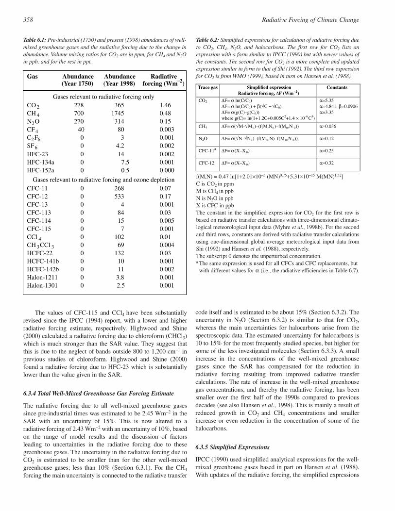
The values of CFC-115 and CCl4 have been substantiallyrevised since the IPCC (1994) report, with a lower and higherradiative forcing estimate, respectively. Highwood and Shine(2000) calculated a radiative forcing due to chloroform (CHCl3)which is much stronger than the SAR value. They suggest thatthis is due to the neglect of bands outside 800 to 1,200 cm−1 inprevious studies of chloroform. Highwood and Shine (2000)found a radiative forcing due to HFC-23 which is substantiallylower than the value given in the SAR.
6.3.4 Total Well-Mixed Greenhouse Gas Forcing Estimate
The radiative forcing due to all well-mixed greenhouse gasessince pre-industrial times was estimated to be 2.45 Wm−2 in theSAR with an uncertainty of 15%. This is now altered to aradiative forcing of 2.43 Wm−2 with an uncertainty of 10%, basedon the range of model results and the discussion of factorsleading to uncertainties in the radiative forcing due to thesegreenhouse gases. The uncertainty in the radiative forcing due toCO2 is estimated to be smaller than for the other well-mixedgreenhouse gases; less than 10% (Section 6.3.1). For the CH4
forcing the main uncertainty is connected to the radiative transfer
code itself and is estimated to be about 15% (Section 6.3.2). Theuncertainty in N2O (Section 6.3.2) is similar to that for CO2,whereas the main uncertainties for halocarbons arise from thespectroscopic data. The estimated uncertainty for halocarbons is10 to 15% for the most frequently studied species, but higher forsome of the less investigated molecules (Section 6.3.3). A smallincrease in the concentrations of the well-mixed greenhousegases since the SAR has compensated for the reduction inradiative forcing resulting from improved radiative transfercalculations. The rate of increase in the well-mixed greenhousegas concentrations, and thereby the radiative forcing, has beensmaller over the first half of the 1990s compared to previousdecades (see also Hansen et al., 1998). This is mainly a result ofreduced growth in CO2 and CH4 concentrations and smallerincrease or even reduction in the concentration of some of thehalocarbons.
6.3.5 Simplified Expressions
IPCC (1990) used simplified analytical expressions for the well-mixed greenhouse gases based in part on Hansen et al. (1988).With updates of the radiative forcing, the simplified expressions
358 Radiative Forcing of Climate Change
Gas Abundance(Year 1750)
Abundance(Year 1998)
Radiativeforcing (Wm−2)
Gases relevant to radiative forcing onlyCO 2 278 365 1.46CH 4 700 1745 0.48N2O 270 314 0.15CF4 40 80 0.003C2F6 0 3 0.001SF6 0 4.2 0.002HFC-23 0 14 0.002HFC-134a 0 7.5 0.001HFC-152a 0 0.5 0.000
Gases relevant to radiative forcing and ozone depletionCFC-11 0 268 0.07CFC-12 0 533 0.17CFC-13 0 4 0.001CFC-113 0 84 0.03CFC-114 0 15 0.005CFC-115 0 7 0.001CCl 4 0 102 0.01CH 3CCl 3 0 69 0.004HCFC-22 0 132 0.03HCFC-141b 0 10 0.001HCFC-142b 0 11 0.002Halon-1211 0 3.8 0.001Halon-1301 0 2.5 0.001
Table 6.1: Pre-industrial (1750) and present (1998) abundances of well-mixed greenhouse gases and the radiative forcing due to the change inabundance. Volume mixing ratios for CO2 are in ppm, for CH4 and N2Oin ppb, and for the rest in ppt.
Trace gas Simplified expressionRadiative forcing, ∆F (Wm−2)
Constants
CO2 ∆F= α ln(C/C0)∆F= α ln(C/C0) + β(√C − √C0)∆F= α(g(C)–g(C0))where g(C)= ln(1+1.2C+0.005C2+1.4 × 10⁻⁶ C3)
α=5.35α=4.841, β=0.0906α=3.35
CH4 ∆F= α(√M–√M0)–(f(M,N0)–f(M0,N 0)) α=0.036
N2O ∆F= α(√N–√N0)–(f(M 0,N)–f(M 0,N 0)) α=0.12
CFC-11a ∆F= α(X–X 0) α=0.25
CFC-12 ∆F= α(X–X 0) α=0.32
Table 6.2: Simplified expressions for calculation of radiative forcing dueto CO2, CH4, N2O, and halocarbons. The first row for CO2 lists anexpression with a form similar to IPCC (1990) but with newer values ofthe constants. The second row for CO2 is a more complete and updatedexpression similar in form to that of Shi (1992). The third row expressionfor CO2 is from WMO (1999), based in turn on Hansen et al. (1988).
f(M,N) = 0.47 ln[1+2.01×10⁻⁵ (MN)0.75+5.31×10⁻¹⁵ M(MN)1.52]C is CO2 in ppmM is CH4 in ppbN is N2O in ppbX is CFC in ppbThe constant in the simplified expression for CO2 for the first row isbased on radiative transfer calculations with three-dimensional climato-logical meteorological input data (Myhre et al., 1998b). For the secondand third rows, constants are derived with radiative transfer calculationsusing one-dimensional global average meteorological input data fromShi (1992) and Hansen et al. (1988), respectively.The subscript 0 denotes the unperturbed concentration.a The same expression is used for all CFCs and CFC replacements, but
with different values for α (i.e., the radiative efficiencies in Table 6.7).
need to be reconsidered, especially for CO2 and N2O. Shi (1992)investigated simplified expressions for the well-mixedgreenhouse gases and Hansen et al. (1988, 1998) presented asimplified expression for CO2. Myhre et al. (1998b) used theprevious IPCC expressions with new constants, finding goodagreement (within 5%) with high spectral resolution radiativetransfer calculations. The already well established and simplefunctional forms of the expressions used in IPCC (1990), andtheir excellent agreement with explicit radiative transfer calcula-tions, are strong bases for their continued usage, albeit withrevised values of the constants, as listed in Table 6.2. Shi (1992)has suggested more physically based and accurate expressionswhich account for (i) additional absorption bands that could yielda separate functional form besides the one in IPCC (1990), and(ii) a better treatment of the overlap between gases. WMO (1999)used a simplified expression for CO2 based on Hansen et al.(1988) and this simplified expression is used in the calculationsof GWP in Section 6.12. For CO2 the simplified expressions fromShi (1992) and Hansen et al. (1988) are also listed alongside theIPCC (1990)-like expression for CO2 in Table 6.2. Compared toIPCC (1990) and the SAR and for similar changes in the concen-trations of well-mixed greenhouse gases, the improved simplifiedexpressions result in a 15% decrease in the estimate of theradiative forcing by CO2 (first row in Table 6.2), a 15% decreasein the case of N2O, an increase of 10 to 15% in the case of CFC-11 and CFC-12, and no change in the case of CH4.
6.4 Stratospheric Ozone
6.4.1 Introduction
The observed stratospheric O3 losses over the past two decadeshave caused a negative forcing of the surface-troposphere system(IPCC, 1992, 1994; SAR). In general, the sign and magnitude ofthe forcing due to stratospheric O3 loss are governed by thevertical profile of the O3 loss from the lower through to the upperstratosphere (WMO, 1999). Ozone depletion in the lower strato-sphere, which occurs mainly in the mid- to high latitudes is theprincipal component of the forcing. It causes an increase in thesolar forcing of the surface-troposphere system. However, thelong-wave effects consist of a reduction of the emission from thestratosphere to the troposphere. This comes about due to the O3
loss, coupled with a cooling of the stratospheric temperatures inthe stratospheric adjustment process, with a colder stratosphereemitting less radiation. The long-wave effects, after adjustment ofthe stratospheric temperatures to the imposed perturbation,overwhelm the solar effect i.e., the negative long-wave forcingprevails over the positive solar to lead to a net negative radiativeforcing of the surface-troposphere system (IPCC, 1992). Themagnitude of the forcing is dependent on the loss in the lowerstratosphere, with the estimates subject to some uncertainties inview of the fact that detailed observations on the vertical profilein this region of the atmosphere are difficult to obtain.
Typically, model-based estimates involve a local (i.e., overthe grid box of the model) adjustment of the stratosphere (Section6.1) assuming the dynamical heating to be fixed (FDH approxi-mation; see also Appendix 6.1). An improved version of this
scheme is the so-called seasonally evolving fixed dynamicalheating (SEFDH; Forster et al., 1997; Kiehl et al., 1999). Theadjustment of the stratosphere to a new thermal equilibrium stateis a critical element for estimating the sign and magnitude of theforcing due to stratospheric O3 loss (WMO, 1992, 1995). Whilethe computational procedures are well established for the FDHand SEFDH approximations in the context of the surface-troposphere forcing, one test of the approximations lies in thecomparison of the computed with observed temperature changes,since it is this factor that plays a large role in the estimate of theforcing. While the temperature changes going into the determi-nation of the forcing are broadly consistent with the observations,there are challenges in comparing quantitatively the actualtemperature changes (which undoubtedly are affected by otherinfluences and may even contain feedbacks due to O3 and otherforcings) with the FDH or SEFDH model simulations (whichnecessarily do not contain feedback effects other than the strato-spheric temperature response due to the essentially radiativeadjustment process).
We reiterate both the concept of the forcing for stratosphericO3 changes and the fact that this has led to a negative radiativeforcing since the late 1970s. Further, the model-based estimatesthat necessarily rely on satellite observations of O3 losses arelikely the most reliable means to derive the forcing, notwith-standing the uncertainty in the vertical profile of loss in thevicinity of the tropopause. Since several model estimates haveemployed the Total Ozone Mapping Spectrometer (TOMS)observations as one of the inputs for the calculations, there is thelikelihood of a small tropospheric O3 change component contam-inating the stratospheric O3 loss amounts, especially for thelowermost regions of the lower stratosphere (Hansen et al.,1997a; Shine and Forster, 1999). Both the estimates derived inthe earlier IPCC assessments and the studies since the SAR showthat the forcing pattern increases from the mid- to high latitudesconsistent with the O3 loss amounts. Seasonally, thewinter/springtime forcings are the largest, again consistent withthe temporal nature of the observed O3 depletion.
It is logical to enquire into the realism of the computedcoolings with the available observations using models morerealistic than FDH/SEFDH, namely GCMs. Furthermore,comparison of the FDH and SEFDH derived temperaturechanges with those from a GCM constitutes another test of theapproximations. WMO (1999) concluded, on the basis ofintercomparisons of the temperature records as measured bydifferent instruments, that there has been a distinct cooling of theglobal mean temperature of the lower stratosphere over the pasttwo decades, with a value of about 0.5°C/decade. Model simula-tions from GCMs using the observed O3 losses yield global meantemperature changes that are approximately consistent with theobservations. Such a cooling is also much larger than that due tothe well-mixed greenhouse gases taken together over the sametime period. Although the possibility of other trace species alsocontributing to this cooling cannot be ruled out, the consistencybetween observations and model simulations enhances thegeneral principle of an O3-induced cooling of the lower strato-sphere, and thus the negativity of the radiative forcing due to theO3 loss. Going from global, annual mean to zonal, seasonal mean
359Radiative Forcing of Climate Change
changes in the lower stratosphere, the agreement between modelsand observations tends to be less strong than for the global meanvalues, but the suggestion of an O3-induced signal exists. Notethough that water vapour changes could also be contributing (seeSection 6.6.4; Forster and Shine, 1999), complicating the quanti-tative attribution of the cooling solely due to O3. As far as theFDH models that have been employed to derive the forcing areconcerned, their temperature changes are broadly consistent withthe GCMs and the observed cooling. However, the mid- to highlatitude cooling in FDH tends to be stronger than in the GCMsand is more than that observed. The SEFDH approximation tendsto do better than the FDH calculation when compared againstobservations (Forster et al., 1997).
6.4.2 Forcing Estimates
Earlier IPCC reports had quoted a value of about −0.1 Wm−2/decade with a factor of two uncertainty. There have beenrevisions in this estimate based on new data available on the O3
trends (Harris et al., 1998; WMO, 1999), and an extension ofthe period over which the forcing is computed. Models usingobserved O3 changes but with varied methods to derive thetemperature changes in the stratosphere have obtained −0.05 to−0.19 Wm−2/decade (WMO, 1999).
Hansen et al. (1997a) have extended the calculations toinclude the O3 loss up to the mid-1990s and performed a varietyof O3 loss experiments to investigate the forcing and response. Inparticular, they obtained forcings of −0.2 and −0.28 Wm−2 for theperiod 1979 to 1994 using SAGE/TOMS and SAGE/SBUVsatellite data, respectively. Hansen et al. (1998) updated theirforcing to −0.2 Wm−2 with an uncertainty of 0.1 Wm−2 for theperiod 1970 to present. Forster and Shine (1997) obtainedforcings of −0.17 Wm−2 and –0.22 Wm−2 for the period 1979 to1996 using SAGE and SBUV observations, respectively. TheWMO (1999) assessment gave a value of −0.2 Wm−2 with anuncertainty of ± 0.15 Wm−2 for the period from late 1970s to mid-1990s. Forster and Shine (1997) have also extended the computa-tions back to 1964 using O3 changes deduced from surface-basedobservations; combining these with an assumption that thedecadal rate of change of forcing from 1979 to 1991 wassustained to the mid-1990s yielded a total stratospheric O3
forcing of about −0.23 Wm−2. Shine and Forster (1999) haverevised this value to −0.15 Wm−2 for the period 1979 to 1997,choosing not to include the values prior to 1979 in view of the lackof knowledge on the vertical profile which makes the sign of thechange also uncertain. They also revised the uncertainty to ± 0.12Wm−2 around the central estimate. A more recent estimate byForster (1999) yields −0.10 ± 0.02 Wm−2 for the 1979 to 1997period using the SPARC O3 profile (Harris et al., 1998).
There have been attempts to use satellite-observed O3 andtemperature changes to gauge the forcing. Thus, Zhong et al.(1996, 1998) obtained a small value of −0.02 Wm−2/decade; andwith inclusion of the 14 micron band, a value of −0.05 Wm−2/decade. It has been noted that the poor vertical resolution of thesatellite temperature retrievals makes it difficult to estimate theforcing; in fact, a similar calculation using radiosonde-basedtemperatures yields a value of −0.1 Wm−2/decade (Shine et al.,
1998). The main difficulty is that the temperature change in thevicinity of the lower stratosphere critically affects the emissionfrom the stratosphere into the troposphere. Thus any uncertaintyin the MSU satellite retrieval induced by the broad altitudeweighting function (see WMO, 1999) becomes an importantfactor in the estimation of the forcing. Further, the degree ofresponse of the climate system, embedded in the observedtemperature change (i.e., feedbacks), is not resolved in an easymanner. This makes it difficult to distinguish quantitatively thepart of temperature change that is a consequence of the strato-spheric adjustment process (which would be, by definition, alegitimate component of the forcing estimate) and that which isdue to mechanisms other than O3 loss. Thus, using observedtemperatures to estimate the forcing may be more uncertain thanthe model-based estimates. It must be noted though that bothmethods share the difficulty of quantifying the vertical andgeographical distributions of the O3 changes near the tropopause,and the rigorous association of this to the observed temperaturechanges. In an overall sense, it is a difficult task to verify theradiative forcing in cases where the stratospheric adjustmentyields a dramatically different result than the instantaneousforcing i.e., where the species changes affect stratospherictemperatures and alter substantially the long-wave radiativeeffects at the tropopause. A related point is the possible upwardmovement of the tropopause which could explain in part theobserved negative trends in O3 and temperature (Fortuin andKelder, 1996).
Kiehl et al. (1999) obtained a radiative forcing of −0.187Wm−2 using the O3 profile data set describing changes since thelate 1970s due to stratospheric depletion alone, consistent withthe range of other models (see Shine et al., 1995). Kiehl et al.(1999) also present results using a very different set of O3 changeprofiles deduced from satellite-derived total column O3 andsatellite-inferred tropospheric O3 measurements to arrive at animplied O3 forcing, considering changes at and above thetropopause, of –0.01 Wm−2. The reason for the considerablyweaker estimate reflects the increased O3 in the tropopauseregion that is believed to have occurred since pre-industrial times(largely before 1970) in many polluted areas. How the changes inO3 at the tropopause are prescribed is hence an important factorfor the difference between this calculation and those from theother estimates.
Clearly, since WMO (1992), this forcing has been investi-gated in an intensive manner using different approaches, and theobservational evidence of the O3 losses, including the spatial andseasonal characteristics, are now on a firmer footing. In arrivingat a best estimate for the forcing, we rely essentially on thestudies that have made use of stratospheric O3 observationsdirectly. Based on this consideration, we adopt here a forcing of−0.15 ± 0.1 Wm−2 for the 1979 to 1997 period. However, it iscautioned that the small values obtained by the two specificstudies mentioned above inhibit the placement of a highconfidence in the estimate quoted.
In general, the reliability of the estimates above is affectedby the fact that the O3 changes in the lower stratosphere,tropopause, and upper troposphere are all poorly quantified,around the globe in general, such that the entire global domain
360 Radiative Forcing of Climate Change
from 200 to 50 hPa becomes crucial for the temperature changeand the adjusted forcing. Forster and Shine (1997) note that thesensitivity of forcing to percentage of O3 loss near the tropopauseis more than when the changes occur lower in the atmosphere.
Myhre et al. (1998a) derived O3 changes using a chemicalmodel in contrast to observations. As the loss of O3 in the upperstratosphere in the simulations was large, a positive forcing of0.02 Wm−2/decade was obtained (see Ramanathan and Dickinson(1979) for an explanation of the change of sign for a O3 loss inthe lower stratosphere versus the upper stratosphere). While thereare difficulties in modelling the O3 depletion in the global strato-sphere (WMO, 1999), this study reiterates the need to becognisant of the role played by the vertical profile of O3 lossamounts in the entire stratosphere, i.e., middle and upper strato-sphere as well, besides the lower stratosphere.
An important issue is whether the actual surface temperatureresponses to the forcing by stratospheric O3 has the samerelationship with forcing as obtained for, say, CO2 or solarconstant changes. Hansen et al. (1997a) and Christiansen (1999)have performed a host of GCM experiments to test this concept.The forcing by lower stratospheric O3 is an unusual one in that ithas a positive short-wave and a negative long-wave radiativeforcing. Moreover, it has a unique vertical structure owing to thefact that the short-wave effects are felt at the surface while thelong-wave is felt only initially at the upper troposphere(Ramanathan and Dickinson, 1979; WMO, 1992). Compared to,say, CO2 change, the stratospheric O3 forcing is not global inextent, being very small in the tropics and increasing from mid-to high latitudes; the O3 forcing also differs in its verticalstructure, since the radiative forcings for CO2 change in both thetroposphere and surface are of the same sign (WMO, 1986). Therelationship between the global mean forcing and responsediffers by less than 20% for O3 profiles, resembling somewhat theactual losses (Hansen et al., 1997a). However, serious departuresoccur if the O3 changes are introduced near surface layers whenthe lapse rate change, together with cloud feedbacks, make theclimate sensitivity quite different from the nominal values. Therealso occur substantial differences in the climate sensitivityparameter for O3 losses in the upper stratosphere. This is furthersubstantiated by Christiansen (1999) who shows that the higherclimate sensitivity for upper stratospheric O3 losses relative tolower stratospheric depletion is related to the vertical partitioningof the forcing, in particular the relative roles of short-wave andlong-wave radiation in the surface-troposphere system. It isencouraging that the global mean climate sensitivity parameterfor cases involving lower stratospheric O3 changes and that forCO2 changes (viz., doubling) are reasonably similar inChristiansen (1999) while being within about 25% of a centralvalue in Hansen et al. (1997a). An energy balance model study(Bintanja et al., 1997) suggests a stronger albedo feedback for O3
changes than for CO2 perturbations (see also WMO, 1999).The evolution of the forcing due to stratospheric O3 loss
hinges on the rate of recovery of the ozone layer, with specialregards to the spatial structure of such a recovery in the mid- tohigh latitudes. If the O3 losses are at their maximum or will reacha maximum within the next decade, then the forcing may notbecome much more negative (i.e., it was −0.1 Wm−2 for just the
1980s; inclusion of the 1990s increases the magnitude by about50%). And, as the O3 layer recovers, the forcing may remainstatic, eventually tending to become less negative. At this time,there will be a lesser offset of the positive greenhouse effects ofthe halocarbons and the other well-mixed greenhouse gases(WMO, 1999). Solomon and Daniel (1996) point out that theglobal mean stratospheric O3 forcing can be expected to scaledown substantially in importance relative to the well-mixedgreenhouse gases, in view of the former’s decline and the latter’ssustained increase in concentrations. Note, however, that theevolution of the negativity of the stratospheric O3 forcing mayvary considerably with latitude and season i.e., the recovery maynot occur at all locations and seasons at the same rate. Thus, thespatial and seasonal evolution of forcing in the future requires asmuch scrutiny as the global mean estimate.
6.5 Radiative Forcing by Tropospheric Ozone
6.5.1 Introduction
Human activities have long been known to influence troposphericO3, not only in urban areas where O3 is a major component of‘smog’, but also in the remote atmosphere (e.g., IPCC, l990,l994; the SAR and references therein). The current state ofscientific understanding of tropospheric O3 chemistry and trendsis reviewed in Chapter 4 of this report, where it is emphasised thattropospheric O3 has an average lifetime of the order of weeks.This relatively short lifetime implies that the distribution oftropospheric O3, as well as the trends in that distribution (whichin turn lead to radiative forcing) are highly variable in space andtime. Studies relating to the evaluation of radiative forcing due toestimated tropospheric O3 increases since pre-industrial times arediscussed here. While there are a number of sites where highquality surface measurements of O3 have been obtained for a fewdecades, there are fewer locations where ozonesonde data allowstudy of the vertical distribution of the trends, and fewer still withrecords prior to about l970. A limited number of surface measure-ments in Europe date back to the late l9th century. These suggestthat O3 has more than tripled in the 20th century there (Marencoet al., l994). The lack of global information on pre-industrialtropospheric O3 distributions is, however, a major uncertainty inthe evaluation of the forcing of this key gas (see Chapter 4).
Biomass burning plays a significant role in tropospheric O3
production and hence in tropical radiative forcing over largespatial scales, particularly in the tropical Atlantic west of thecoast of Africa (e.g., Fishman, l99l; Fishman and Brackett, l997;Portmann et al., l997; Hudson and Thompson, l998) and inIndonesia (Hauglustaine et al., l999). Export of industrialpollution to the Arctic can lead to increased O3 over a highlyreflective snow or ice surface, and correspondingly large localradiative forcings (Hauglustaine et al., 1998; Mickley et al.,1999).
Chapter 4 and Sections 6.6.2 and 6.6.3 discuss the chemistryresponsible for the tropospheric O3 forcing; here we emphasisethat the tropospheric O3 forcing is driven by and broadly attribut-able to emissions of other gases. The observed regionalvariability of O3 trends is related to the transport of key precur-
361Radiative Forcing of Climate Change
sors, particularly reactive nitrogen, CO, and NMHCs (seeChapter 4). However, the chemistry of O3 production can be non-linear, so that increased emissions of, for example, the nitricoxide precursor do not necessarily lead to linear responses in O3
concentrations over all ranges of likely values (e.g, Kleinman,l994; Klonecki and Levy, l997). Further, the relationship ofprecursor emissions to O3 trends may also vary in time. Onestudy suggests that the O3 production efficiency per mole ofnitrogen oxide emitted has decreased globally by a factor of twosince pre-industrial times (Wang and Jacob, l998). Because ofthese complex and poorly understood interactions, the forcingdue to tropospheric O3 trends cannot be reliably and uniquelyattributed in a quantitative fashion to the emissions of specificprecursors.
For the purposes of this report, several evaluations of theglobal radiative forcing due to tropospheric O3 changes sincepre-industrial times have been intercompared. It will be shownthat the uncertainties in radiative forcing can be betterunderstood when both the absolute radiative forcing (Wm−2)and normalised forcing (Wm−2 per Dobson Unit of troposphericO3 change) are considered. The results of this intercomparisonand the availability of numerous models using differentapproaches suggest reduced uncertainties in the radiativeforcing estimates compared to those of the SAR. Furthermore,recent work has shown that the dependence of the forcing on thealtitude where the O3 changes occur within the troposphere isless pronounced than previously thought, providing improvedscientific understanding. Finally, some estimates of the likelymagnitude of future tropospheric O3 radiative forcing arepresented and discussed.
6.5.2 Estimates of Tropospheric Ozone Radiative Forcing since Pre-Industrial Times
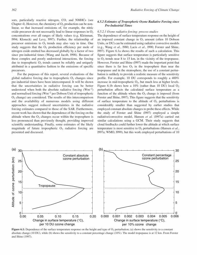
6.5.2.1 Ozone radiative forcing: process studiesThe dependence of surface temperature response on the height ofan imposed constant change in O3 amount (often 10 DobsonUnits, or DU) can be estimated using radiative convective models(e.g., Wang et al., l980; Lacis et al., l990; Forster and Shine,l997). Figure 6.1a shows the results of such a calculation. Thisfigure suggests that surface temperature is particularly sensitiveto O3 trends near 8 to 15 km, in the vicinity of the tropopause.However, Forster and Shine (l997) made the important point thatsince there is far less O3 in the troposphere than near thetropopause and in the stratosphere, the use of a constant pertur-bation is unlikely to provide a realistic measure of the sensitivityprofile. For example, 10 DU corresponds to roughly a 400%increase in mid-tropospheric O3, but much less at higher levels.Figure 6.1b shows how a 10% (rather than 10 DU) local O3
perturbation affects the calculated surface temperature as afunction of the altitude where the O3 change is imposed (fromForster and Shine, l997). This figure suggests that the sensitivityof surface temperature to the altitude of O3 perturbations isconsiderably smaller than suggested by earlier studies thatemployed constant absolute changes to probe these effects. Whilethe study of Forster and Shine (l997) employed a simpleradiative/convective model, Hansen et al. (l997a) carried outsimilar calculations using a GCM. Their study suggests thatcloud feedbacks could further lower the altitude at which surfacetemperature is most sensitive to O3 perturbations (Hansen et al.,l997a; WMO, l999), but this work employed perturbations of 10
362 Radiative Forcing of Climate Change
0.200.150.100.050
5
10
15
20
25
30
0.00
(a) (b)
Change in surface temperature (°C), Change in surface temperature (°C), per 10 DU ozone change
Alti
tude
of
ozon
e pe
rtur
batio
n (k
m) Constant absolute
ozone perturbation
Tropopause
0.0060.0050.0040.0030.0020.0010.0000
5
10
15
20
25
30
per 10% ozone change
Constant percentageozone perturbation
Figure 6.1: Dependence of the surface temperature response on the height and type of O3 perturbation; (a) shows the sensitivity to a constantabsolute change (10 DU), while (b) shows the sensitivity to a constant percentage change (10%). The model tropopause is at 12 km. From Forsterand Shine (1997).

DU in each layer (which is necessary to obtain a significantsignal in the GCM but is, as noted above, an unrealistically largevalue for the tropospheric levels in particular).
Portmann et al. (l997) and Kiehl et al. (l999) combined anO3 climatology based upon satellite measurements of the tropo-spheric column content (from Fishman and Brackett, l997) witha model calculation to derive estimates of the O3 radiative forcingfor the tropics and for the globe, respectively. They showed thatthe dependence of the normalised O3 forcing (Wm−2 per DU ofintegrated O3 column change) upon uncertainties in the verticaldistribution of the perturbation was less than previously thought,about 0.03 to 0.06 Wm−2 per DU based upon their radiative codeand considering a range of profile shapes. This rather limitedsensitivity to the altitude distribution of the imposed perturbationis broadly consistent with the work of Forster and Shine (l997)highlighted above and in Figure 6.1.
6.5.2.2 Model estimatesTable 6.3 presents a comparison of estimates of globally averagedO3 change since pre-industrial times and its correspondingradiative forcing based on published literature and includingstratospheric temperature adjustment. Results from severalstudies are presented, one constrained by the climatology derivedfrom observations discussed in the previous section, and ten fromglobal chemistry/transport models. Results are presented for bothclear sky and for total sky conditions, providing an indication ofthe role of clouds, and long-wave and short-wave contributionsare shown separately. In addition, the globally averagedintegrated tropospheric O3 change (DU) is also indicated, to givea sense of the range in published model estimates of this key
factor. Finally, the normalised O3 forcings are also presented(Wm−2 per DU).
Table 6.3 summarises the ranges obtained in these modelstudies. For total sky conditions, the range in globally and annualaveraged tropospheric O3 forcing from all of these models is from0.28 to 0.43 Wm−2, while the normalised forcing is 0.033 to0.056 Wm−2 per DU. The tropospheric O3 forcing constrained bythe observational climatology is 0.32 Wm−2 for globallyaveraged, total sky conditions. These estimates are comparable inmagnitude (and qualitatively similar in pattern, see Section 6.14)but opposite in sign to that believed to be due to the direct effectof sulphate aerosols.
Figure 6.2 presents the latitudinal distributions of absoluteand normalised forcings for both January and July, from severalchemistry/transport models and from the observationallyconstrained evaluation. The figure shows that the tropics andnorthern mid-latitude regions account for the bulk of the globalforcing. The contribution from northern mid-latitudes is particu-larly large in summer, when it can reach as much as 1 Wm−2
locally near 40 to 50°N. These latitudinal gradients and seasonalchanges in the zonally-averaged forcing are likely to be reflectedat least in part in patterns of response (Hansen et al., l997a) andhence are a needed element in the detection and attribution ofclimate change.
Figure 6.2 shows that the large seasonal and inter-modelranges in absolute forcings compress somewhat when normalisedforcings are considered. At 40°N for example, the absoluteforcing differs over all models and seasons by more than a factorof 5 (Figure 6.2a), while the differences in normalised forcingsare about a factor of 2.5 (Figure 6.2b). Mickley et al. (1999)
363Radiative Forcing of Climate Change
Clear sky conditions Total sky conditions
Reference ∆O3 LW SW SW(norm.)
Net Net(norm.)
LW SW Net Net(norm.)
Berntsen et al. (1997) –[Reading model]
7.600 0.260 0.050 0.007 0.310 0.041 0.210 0.070 0.280 0.037
Stevenson et al. (1998) 8.700 0.326 0.065 0.007 0.391 0.045 0.201 0.088 0.289 0.033Berntsen et al. (1997) –
[Oslo model]7.600 0.330 0.060 0.008 0.390 0.051 0.230 0.080 0.310 0.041
Haywood et al. (1998a) 7.900 0.330 0.050 0.006 0.380 0.048 0.230 0.080 0.310 0.039Kiehl et al. (1999) 8.400 0.316 0.063 0.008 0.379 0.045 0.251 0.069 0.320 0.038Berntsen et al. (2000) 9.600 0.357 0.071 0.007 0.428 0.045 0.246 0.096 0.342 0.036Brasseur et al. (1998) – – – – – – – – 0.370 –van Dorland et al. (1997) 8.070 0.390 0.054 0.007 0.443 0.055 0.304 0.076 0.380 0.047Roelofs et al. (1997) 7.200 0.350 0.047 0.007 0.397 0.055 0.287 0.117 0.404 0.056Lelieveld and Dentener (2000) – – – – – – – – 0.420 –Hauglustaine et al. (1998) 8.940 0.448 0.063 0.007 0.511 0.057 0.338 0.088 0.426 0.048
Mean 8.224 0.345 0.058 0.007 0.403 0.049 0.255 0.085 0.343 0.042
Table 6.3: Tropospheric O3 change (∆O3) in Dobson Units (DU) since pre-industrial times, and the accompanying short-wave (SW), long-wave (LW),and net (SW plus LW) radiative forcings (Wm−2), after accounting for stratospheric temperature adjustment (using the Fixed Dynamical Heatingmethod). Estimates are taken from the published literature. Normalised forcings (norm.) refer to radiative forcing per O3 change (Wm−2 per DU).
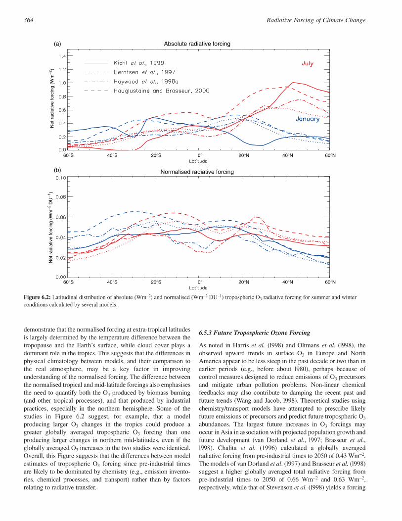
demonstrate that the normalised forcing at extra-tropical latitudesis largely determined by the temperature difference between thetropopause and the Earth’s surface, while cloud cover plays adominant role in the tropics. This suggests that the differences inphysical climatology between models, and their comparison tothe real atmosphere, may be a key factor in improvingunderstanding of the normalised forcing. The difference betweenthe normalised tropical and mid-latitude forcings also emphasisesthe need to quantify both the O3 produced by biomass burning(and other tropical processes), and that produced by industrialpractices, especially in the northern hemisphere. Some of thestudies in Figure 6.2 suggest, for example, that a modelproducing larger O3 changes in the tropics could produce agreater globally averaged tropospheric O3 forcing than oneproducing larger changes in northern mid-latitudes, even if theglobally averaged O3 increases in the two studies were identical.Overall, this Figure suggests that the differences between modelestimates of tropospheric O3 forcing since pre-industrial timesare likely to be dominated by chemistry (e.g., emission invento-ries, chemical processes, and transport) rather than by factorsrelating to radiative transfer.
6.5.3 Future Tropospheric Ozone Forcing
As noted in Harris et al. (l998) and Oltmans et al. (l998), theobserved upward trends in surface O3 in Europe and NorthAmerica appear to be less steep in the past decade or two than inearlier periods (e.g., before about l980), perhaps because ofcontrol measures designed to reduce emissions of O3 precursorsand mitigate urban pollution problems. Non-linear chemicalfeedbacks may also contribute to damping the recent past andfuture trends (Wang and Jacob, l998). Theoretical studies usingchemistry/transport models have attempted to prescribe likelyfuture emissions of precursors and predict future tropospheric O3
abundances. The largest future increases in O3 forcings mayoccur in Asia in association with projected population growth andfuture development (van Dorland et al., l997; Brasseur et al.,l998). Chalita et al. (1996) calculated a globally averagedradiative forcing from pre-industrial times to 2050 of 0.43 Wm−2.The models of van Dorland et al. (l997) and Brasseur et al. (l998)suggest a higher globally averaged total radiative forcing frompre-industrial times to 2050 of 0.66 Wm−2 and 0.63 Wm−2,respectively, while that of Stevenson et al. (l998) yields a forcing
364 Radiative Forcing of Climate Change
Absolute radiative forcingN
et r
adia
tive
forc
ing
(Wm
−2)
Net
rad
iativ
e fo
rcin
g (W
m−2
DU
−1)
60°S 40°S 20°S 0° 20°N 40°N 60°N
60°S 40°S 20°S 0° 20°N 40°N 60°N
(a)
(b) Normalised radiative forcing
Figure 6.2: Latitudinal distribution of absolute (Wm−2) and normalised (Wm−2 DU−1) tropospheric O3 radiative forcing for summer and winterconditions calculated by several models.
of 0.48 Wm−2 in 2100. As the analysis presented above shows,these differences are likely to be due to modelled differences inthe latitudinal distributions or magnitudes of the projected O3
change due for example to different emission inventories ormodel processes such as transport, and much less likely to be dueto differences in radiative codes.
6.6 Indirect Forcings due to Chemistry
In addition to the direct forcings caused by injection ofradiatively active gases to the atmosphere, some compounds orprocesses can also modify the radiative balance through indirecteffects relating to chemical transformation or change in the distri-bution of radiatively active species. As previously indicated(IPCC, 1992, 1994; SAR), the tropospheric chemical processesdetermining the indirect greenhouse effects are highly complexand not fully understood. The uncertainties connected withestimates of the indirect effects are larger than the uncertaintiesof those connected to estimates of the direct effects. Because ofthe central role that O3 and OH play in tropospheric chemistry,the chemistry of CH4, CO, NMHC, and NOx is stronglyintertwined, making the interpretation of the effects associatedwith emission changes rather complex. It should be noted thatindirect effects involving OH feedback on the lifetime of well-mixed greenhouse gases, and tropospheric O3 concentrationchanges since the pre-industrial are implicitly accounted for inSections 6.3 and 6.5.
6.6.1 Effects of Stratospheric Ozone Changes on Radiatively Active Species
Increased penetration of ultraviolet radiation into the troposphereas a result of stratospheric ozone depletion leads to changes in thephotodissociation rates of some key chemical species. One of theprimary species affected by possible changes in photodissocia-tion rates is the hydroxyl radical OH, which regulates the tropos-pheric lifetime of a large number of trace gases such as CH4, CO,hydrochlorofluorocarbons (HCFCs), hydrofluorocarbons (HFCs),NOx, and to a lesser extent, sulphur dioxide (SO2) (see Chapter4). The impact of stratospheric O3 changes on the fate of tropo-spheric species has been discussed by Ma and van Weele (2000),Fuglestvedt et al. (1994), Bekki et al. (1994); and Fuglestvedt etal. (1995); on the basis of two-dimensional model simulations,and by Madronich and Granier (1994), Granier et al. (1996), VanDop and Krol (1996) and Krol et al. (1998) using three-dimensional models. These studies and the updated calculationspresented by WMO (1999) estimated that a 1% decrease inglobal total O3 leads to a global increase in O3 photolysis rateof 1.4%, resulting in a 0.7 to 0.8% increase in global OH.Changes in photolysis rates from reduced stratospheric O3
also have the potential to alter tropospheric O3 production anddestruction rates. Based on stratospheric O3 evolution over theperiod 1980 to 1996, Myhre et al. (2000) have calculated areduction in tropospheric O3 associated with increased ultra-violet penetration and a corresponding negative radiativeforcing reaching −0.01 Wm−2 over that period of time.Another indirect impact of stratospheric O3 depletion on
climate forcing has been proposed by Toumi et al. (1994,1995). The hydroxyl radical oxidises SO2 to gaseous sulphuricacid, which is a source of H2SO4 particles. Changes in H2SO4
formation resulting from OH changes might affect the numberof particles which act as condensation nuclei. Rodhe andCrutzen (1995) challenged whether this mechanism was ofimportance.
6.6.2 Indirect Forcings of Methane, Carbon Monoxide and Non-Methane Hydrocarbons
CH4 is oxidised primarily (>90%) in the troposphere throughreaction with OH. Since the CH4 oxidation cycle provides asubstantial fraction of the OH loss in the troposphere, there isstrong interaction between OH and CH4. This causes the OH todecrease when CH4 increases, leading to a further increase inCH4. This chemical feedback is examined in Chapter 4. Lelieveldand Crutzen (1992), Brühl (1993), Lelieveld et al. (1993, 1998),Hauglustaine et al. (1994) and Fuglestvedt et al. (1996) estimatedthat this feedback added 25 to 35% to the direct CH4 forcingdepending on the initial CH4 perturbation and the model used.These values are in line with the 30% contribution estimated byIPCC (1992) and the SAR. The tropospheric O3 increaseassociated with photochemical production from the CH4
oxidation cycle also contributes to enhancing the total CH4
radiative forcing. The forcing from enhanced levels of tropo-spheric O3 estimated by Lelieveld and Crutzen (1992),Lelieveld et al. (1993, 1998), Hauglustaine et al. (1994) andFuglestvedt et al. (1996) contributes a further 30 to 40% on topof the CH4 forcing, due directly to CH4 emissions. IPCC (1992)estimated a lower contribution of O3 of approximately 20%.Lelieveld et al. (1998) have estimated a direct radiative forcingassociated with CH4 increase since the pre-industrial era (1850 to1992) of 0.33 Wm−2 and an additional forcing of 0.11 Wm−2
associated with OH feedback. The increased tropospheric O3
contributes an additional 0.11 Wm−2 and stratospheric H2Oanother 0.02 Wm−2. These authors found that the total CH4
forcing (0.57 Wm−2) is higher by 73% than the direct forcing.The CH4 radiative forcing given in Section 6.3 (0.5 Wm−2) andbased on recorded CH4 concentration increase includes both thedirect and OH indirect contributions. This updated forcing ishigher by 14% than the 0.44 Wm−2 obtained by Lelieveld et al.(1998) on the basis of calculated present day and pre-industrialCH4 distributions. In addition to that, oxidation of CH4 also leadsto the formation of CO2, providing a further indirect effect.
In contrast to CH4, the direct radiative forcing of CO isrelatively small (Evans and Puckrin, 1995; Sinha and Toumi,1996). Sinha and Toumi (1996) have estimated a clear skyradiative forcing of 0.024 Wm−2 for a uniform increase in COfrom 25 ppbv to 100 ppbv. However, CO plays a primary role ingoverning OH abundances in the troposphere. As indicated byPrather (1994, 1996) and Daniel and Solomon (1998), COemissions into the atmosphere may have a significant impact onclimate forcing due to chemical impact on CH4 lifetime, andtropospheric O3 and CO2 photochemical production (see Chapter4). The contribution of these indirect effects to the GWPs basedon box model calculations are presented in Section 6.12.
365Radiative Forcing of Climate Change
Similarly, NMHCs have a small direct radiative forcing.Highwood et al. (1999) estimated an upper limit of 0.015 Wm−2
(1% of the present day forcing due to other greenhouse gases) onthe globally averaged direct forcing of sixteen NMHCs. Asindicated by Johnson and Derwent (1996), the indirect forcingthrough changes in OH and tropospheric O3 is also small for eachNMHC taken individually but can be significant taken as afamily. The indirect forcings of NMHCs are still poorly quanti-fied and require the use of global three-dimensional chemicaltransport models. Accurate calculations of these effects are anotoriously difficult problem in atmospheric chemistry.
6.6.3 Indirect Forcing by NOx Emissions
Through production of tropospheric O3, emissions of nitrogenoxides (NOx = NO + NO2) lead to a positive radiative forcing ofclimate (warming), but by affecting the concentration of OH theyreduce the levels of CH4, providing a negative forcing (cooling)which partly offsets the O3 forcing. Due to non-linearities in O3
photochemical production together with differences in mixingregimes and removal processes, the O3 and OH changes stronglydepend on the localisation of the NOx surface emission perturba-tion, as calculated by Hauglustaine and Granier (1995), Johnsonand Derwent (1996), Berntsen et al. (1996), Fuglestvedt et al.(1996, 1999) and Gupta et al. (1998). The CH4 and O3 forcingsare similar in magnitude, but opposite in sign, as calculated byFuglestvedt et al. (1999). Due to differences in CH4 and O3
lifetimes, the NOx perturbation on the CH4 forcing acts on aglobal scale over a period of approximately a decade, while theO3 forcing is of regional character and occurs over a period ofweeks. Based on three-dimensional model results, Fuglestvedt etal. (1999) have calculated that the O3 radiative forcing perchange in NOx emission (10−2 Wm−2 per TgN/yr) is 0.35 and0.29 for the USA and Scandinavia, respectively, and reaches 2.4for Southeast Asia. The CH4 forcing per change in NOx emissionranges from −0.37 (Scandinavia) and −0.5 (USA) to −2.3(Southeast Asia) in the same units. Additional work is required toassess the impact of NOx on the radiative forcing of climate.
Deep convection can remove pollutants from the loweratmosphere and inject them rapidly into the middle and uppertroposphere and, occasionally, into the stratosphere. Changes inconvective regimes associated with climate changes havetherefore the potential to significantly modify the distribution andthe photochemistry of O3 in a region where its impact on theradiative forcing is the largest. Based on the tropospheric O3
column derived from satellite during the 1997 to 1998 El Niño,Chandra et al. (1998) reported a decrease in O3 column of 4 to 8Dobson Units (DU) in the eastern Pacific and an increase of 10to 20 DU in the western Pacific, largely as a result of theeastward shift of the tropical convective activity. Lelieveld andCrutzen (1994) showed that convective transport can change thebudget of O3 in the troposphere. Berntsen and Isaksen (1999)have also indicated that changes in convection can modify thesensitivity of the atmosphere to anthropogenic perturbations asaircraft emissions. Their study indicates that reduced convectiveactivity leads to a 40% increase in the O3 response to aircraftNOx emissions due to modified background atmospheric
concentrations. In addition to that, lightning is a major sourceof NOx in the troposphere and thus contributes to thephotochemical production of O3 (Huntrieser et al., 1998; Wanget al., 1998; Hauglustaine et al., 2001; Lelieveld and Dentener,2000). In the tropical mid- and upper troposphere, modellingstudies by Lamarque et al. (1996), Levy et al. (1996), Penner etal. (1998a), and Allen et al. (2000) have calculated a contribu-tion of lightning to the NOx levels of 60 to 90% during summer.Direct observations by Solomon et al. (1999) of absorption ofvisible radiation indicate that nitrogen dioxide can lead to localinstantaneous radiative forcing exceeding 1 Wm−2. Theseenhancements of NO2 absorption are likely to be due both topollution and to production by lightning in convective clouds.Further measurements are required to bracket the direct radiativeforcing by NO2 under a variety of storm and pollution conditions.On the basis of two-dimensional model calculations, Toumi et al.(1996) calculated that for a 20% increase of lightning the globalmean radiative forcing by enhanced tropospheric O3 productionis about 0.1 Wm−2. Based on an apparent correlation betweenlightning strike rates and surface temperatures, Sinha andToumi (1997) have suggested a positive climate feedbackthrough O3 production from lightning NOx in a warmer climate.Improved modelling and observations are required to confirmthis hypothesis.
Aircraft emissions also have the potential to alter thecomposition of the atmosphere and induce a radiative forcing ofclimate. According to IPCC (1999), in 1992 the NOx emissionsfrom subsonic aircraft are estimated to have increased O3
concentrations at cruise altitudes in the Northern Hemispheremid-latitude summer by about 6% compared with an atmospherewithout aircraft. The associated global mean radiative forcing is0.023 Wm−2. In addition to increasing tropospheric O3, aircraftNOx are expected to decrease the concentration of CH4 inducinga negative radiative forcing of −0.014 Wm−2 for the 1992 aircraftfleet. Again, due to different O3 and CH4 lifetimes, the twoforcings show very different spatial distribution and seasonalevolution (IPCC, 1999). The O3 forcing shows a markedmaximum at northern mid-latitudes, reaching 0.06 Wm−2, whilstthe CH4 forcing exhibits a more uniform distribution, with amaximum of about −0.02 Wm−2 in the tropical regions. Based onIPCC (1999), the O3 forcing calculated for 2050 conditions is0.060 Wm−2 and the CH4 forcing is −0.045 Wm−2.
6.6.4 Stratospheric Water Vapour
The oxidation of CH4 produces water vapour that can contributesignificantly to the levels of H2O in the stratosphere. Watervapour is also directly emitted by aircraft in the lower strato-sphere. Lelieveld and Crutzen (1992), Lelieveld et al. (1993,1998), Hauglustaine et al. (1994) and Fuglestvedt et al. (1996)have estimated a contribution of stratospheric water vapour of 2to 5% of the total CH4 forcing. Oltmans and Hofmann (1995)have reported an increase in lower stratospheric H2O (18 to 20km) measured at Boulder of 0.8% per year for the period 1981 to1994. Measurements of stratospheric H2O from the HALOEinstrument on board the UARS satellite also show an increase instratospheric H2O between 30 and 60 km of 40 to 100 ppbv/year
366 Radiative Forcing of Climate Change
for the period 1992 to 1997 (Evans et al., 1998; Nedoluha et al.,1998). A similar trend has also been reported by Randel et al.(1999) based on HALOE data for the period 1993 to 1997. Inthis study, a time variation and a flattening of the trend has beendetermined after 1996. This stratospheric H2O increase is wellabove that expected from the rising CH4 levels in theatmosphere. Based on these observed stratospheric H2O trends,Forster and Shine (1999) have estimated a radiative forcing of0.2 Wm−2 since 1980. Note that, just as for stratospheric O3,there exists considerable uncertainty concerning the trend nearthe tropopause region globally. It should also be noted that if thechanges in water vapour were a result of CH4 oxidation, thechanges in H2O would be a forcing. However, if they resultfrom changes in tropical tropopause temperature change or indynamics, then they should be viewed as a feedback (as definedin Section 6.2). Additional measurements and analyses areclearly needed to explain the observed trends.
6.7 The Direct Radiative Forcing of Tropospheric Aerosols
Anthropogenic aerosols scatter and absorb short-wave and long-wave radiation, thereby perturbing the energy budget of theEarth/atmosphere system and exerting a direct radiative forcing.This section concentrates on estimates of the global mean directeffect of anthropogenic tropospheric aerosols and is necessarilydependent upon global models. Field campaigns which provideessential input parameters for the models, and satellite observa-tional studies of the direct effect of tropospheric aerosols, whichprovide useful validation data for the models, are considered indetail in Chapter 5.
6.7.1 Summary of the IPCC WGI Second Assessment Report and Areas of Development
The SAR considered three anthropogenic aerosol species;sulphate, biomass burning aerosols, and fossil fuel black carbon(or soot). The SAR suggested a radiative forcing of −0.4 Wm−2
with a factor of two uncertainty for sulphate aerosols, −0.2 Wm−2
with a factor of three uncertainty for biomass burning, and +0.1Wm−2 with a factor of three uncertainty for fossil fuel blackcarbon aerosols. The level of scientific understanding (referred toas a confidence level in the SAR, see Section 6.13) was classifiedas “low” for sulphate aerosol and “very low” for both fossil fuelblack carbon and biomass burning aerosols. Since the SAR, therehave been advances in both modelling and observational studiesof the direct effect of tropospheric aerosols (see reviews by Shineand Forster (1999) and Haywood and Boucher (2000)). Globalchemical transport modelling studies encompass a greaternumber of aerosol species and continue to improve the represen-tation of the physical and chemical processes (see Chapters 4 and5). Global models are more numerous and include moreaccurate radiative transfer codes, more sophisticated treatmentsof the effects of relative humidity for hygroscopic aerosols,better treatment of clouds, and better spatial and temporalresolution than some earlier studies. The present day directradiative forcing due to aircraft emissions of sulphate and blackcarbon aerosol have been calculated to be insignificant (IPCC,
1999) and are not considered further. Spatial patterns of thecalculated radiative forcings are not discussed in detail here butare presented in Section 6.14.
6.7.2 Sulphate Aerosol
Early one-dimensional box-model estimates of the radiativeforcing (e.g., Charlson et al., 1992) using simplified expres-sions for radiative forcing have been superseded by globalcalculations using prescribed aerosol concentrations fromchemical transport models (CTMs). These studies use eitherthree-dimensional observed fields of for example, clouds,relative humidity and surface reflectance (e.g., Kiehl andBriegleb, 1993; Myhre et al., 1998c), or GCM generated fields(e.g., Boucher and Anderson, 1995; Haywood et al., 1997a)together with the prescribed aerosol distributions from CTMsand detailed radiative transfer codes in calculating the radiativeforcing. A growing number of studies perform both thechemical production, transformation, and transportation ofaerosols and the radiative forcing calculations (see Chapter 5)with the advantage of correlating predicted aerosol distributionsprecisely with fields determining aerosol production anddeposition such as clouds (e.g., Penner et al., 1998b). Table 6.4summarises estimates of the radiative forcing from globalmodelling studies.
The calculated global mean radiative forcing ranges from−0.26 to −0.82 Wm−2, although most lie in the range −0.26 to−0.4 Wm−2. The spatial distribution of the forcings is similar inthe studies showing strongest radiative forcings over industrialregions of the Northern Hemisphere although the ratio of theannual mean Northern Hemisphere/Southern Hemisphereradiative forcing varies from 2.0 (Graf et al., 1997) to 6.9 (Myhreet al., 1998c) (see Section 6.14.2 for further details). The ratio ofthe annual mean radiative forcing over land to that over oceanalso varies considerably, ranging from 1.3 (Kiehl et al., 2000) to3.4 (Boucher and Anderson, 1995). The direct radiative forcing(DRF) is strongest in the Northern Hemisphere summer when theinsolation is the highest although different seasonal cycles of thesulphate burden from the chemical transport models result inmaximum global mean radiative forcings ranging from May toAugust (e.g., Haywood and Ramaswamy, 1998), the ratio of theJune-July-August/December-January-February radiative forcingbeing estimated to lie in the range less than 2 (e.g., van Dorlandet al., 1997) to > 5 (e.g., Penner et al., 1998b; Grant et al., 1999)with a mean of approximately 3.3. The range of uncertainty inthe radiative forcings can be isolated from the uncertainties inthe simulated sulphate loadings by considering the range in thenormalised radiative forcing i.e., the radiative forcing per unitmass of sulphate aerosol (e.g., Nemesure et al., 1995; Pilinis etal., 1995). Table 6.4 shows that this is substantial, indicatingthat differences in the radiative forcing are not due solely todifferent mass loading.
The optical parameters for sulphate aerosol in each of theglobal studies vary. Although the single scattering albedo of puresulphate and sulphate mixed with water is close to unitythroughout most of the solar spectrum, some of the studies (e.g.,Feichter et al., 1997; van Dorland et al., 1997; Hansen et al.,
367Radiative Forcing of Climate Change
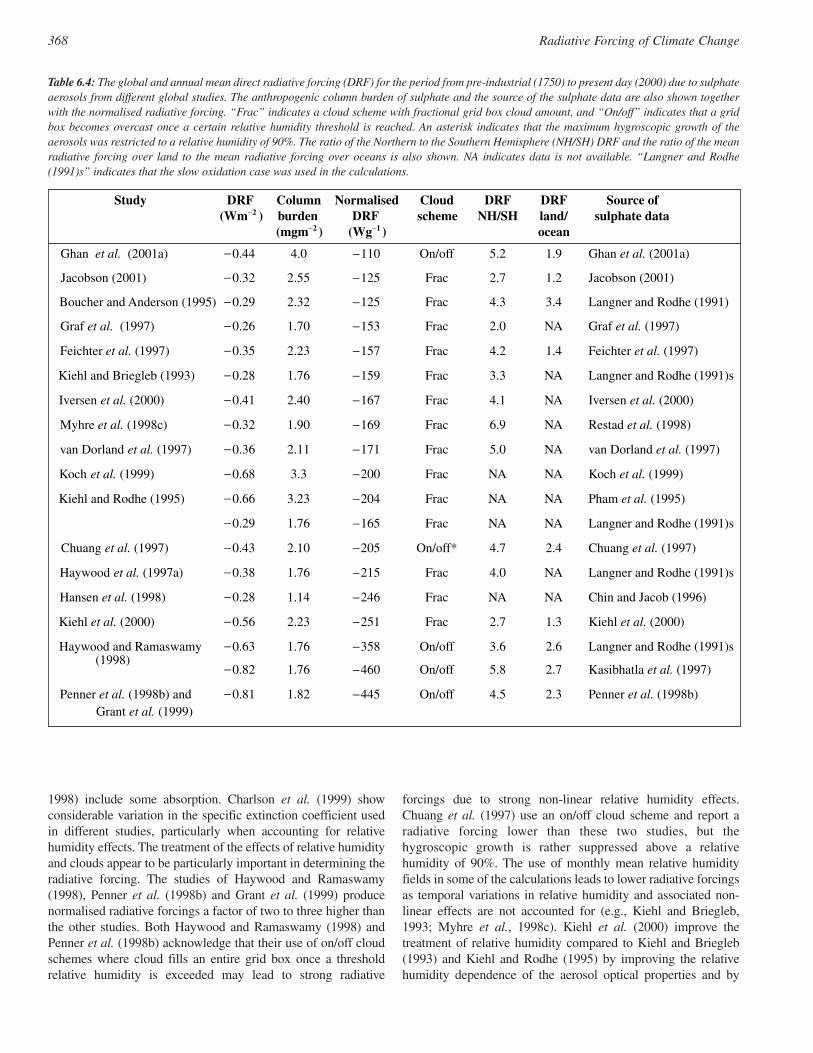
1998) include some absorption. Charlson et al. (1999) showconsiderable variation in the specific extinction coefficient usedin different studies, particularly when accounting for relativehumidity effects. The treatment of the effects of relative humidityand clouds appear to be particularly important in determining theradiative forcing. The studies of Haywood and Ramaswamy(1998), Penner et al. (1998b) and Grant et al. (1999) producenormalised radiative forcings a factor of two to three higher thanthe other studies. Both Haywood and Ramaswamy (1998) andPenner et al. (1998b) acknowledge that their use of on/off cloudschemes where cloud fills an entire grid box once a thresholdrelative humidity is exceeded may lead to strong radiative
forcings due to strong non-linear relative humidity effects.Chuang et al. (1997) use an on/off cloud scheme and report aradiative forcing lower than these two studies, but thehygroscopic growth is rather suppressed above a relativehumidity of 90%. The use of monthly mean relative humidityfields in some of the calculations leads to lower radiative forcingsas temporal variations in relative humidity and associated non-linear effects are not accounted for (e.g., Kiehl and Briegleb,1993; Myhre et al., 1998c). Kiehl et al. (2000) improve thetreatment of relative humidity compared to Kiehl and Briegleb(1993) and Kiehl and Rodhe (1995) by improving the relativehumidity dependence of the aerosol optical properties and by
368 Radiative Forcing of Climate Change
Study DRF(Wm−2 )
Columnburden(mgm−2 )
NormalisedDRF
(Wg−1 )
Cloudscheme
DRFNH/SH
DRFland/ocean
Source ofsulphate data
Ghan et al. (2001a) −0.44 4.0 −110 On/off 5.2 1.9 Ghan et al. (2001a)
Jacobson (2001) −0.32 2.55 −125 Frac 2.7 1.2 Jacobson (2001)
Boucher and Anderson (1995) −0.29 2.32 −125 Frac 4.3 3.4 Langner and Rodhe (1991)
Graf et al. (1997) −0.26 1.70 −153 Frac 2.0 NA Graf et al. (1997)
Feichter et al. (1997) −0.35 2.23 −157 Frac 4.2 1.4 Feichter et al. (1997)
Kiehl and Briegleb (1993) −0.28 1.76 −159 Frac 3.3 NA Langner and Rodhe (1991)s
Iversen et al. (2000) −0.41 2.40 −167 Frac 4.1 NA Iversen et al. (2000)
Myhre et al. (1998c) −0.32 1.90 −169 Frac 6.9 NA Restad et al. (1998)
van Dorland et al. (1997) −0.36 2.11 −171 Frac 5.0 NA van Dorland et al. (1997)
Koch et al. (1999) −0.68 3.3 −200 Frac NA NA Koch et al. (1999)
Kiehl and Rodhe (1995) −0.66 3.23 −204 Frac NA NA Pham et al. (1995)
−0.29 1.76 −165 Frac NA NA Langner and Rodhe (1991)s
Chuang et al. (1997) −0.43 2.10 −205 On/off* 4.7 2.4 Chuang et al. (1997)
Haywood et al. (1997a) −0.38 1.76 −215 Frac 4.0 NA Langner and Rodhe (1991)s
Hansen et al. (1998) −0.28 1.14 −246 Frac NA NA Chin and Jacob (1996)
Kiehl et al. (2000) −0.56 2.23 −251 Frac 2.7 1.3 Kiehl et al. (2000)
Haywood and Ramaswamy(1998)
−0.63 1.76 −358 On/off 3.6 2.6 Langner and Rodhe (1991)s
−0.82 1.76 −460 On/off 5.8 2.7 Kasibhatla et al. (1997)
Penner et al. (1998b) andGrant et al. (1999)
−0.81 1.82 −445 On/off 4.5 2.3 Penner et al. (1998b)
Table 6.4: The global and annual mean direct radiative forcing (DRF) for the period from pre-industrial (1750) to present day (2000) due to sulphateaerosols from different global studies. The anthropogenic column burden of sulphate and the source of the sulphate data are also shown togetherwith the normalised radiative forcing. “Frac” indicates a cloud scheme with fractional grid box cloud amount, and “On/off” indicates that a gridbox becomes overcast once a certain relative humidity threshold is reached. An asterisk indicates that the maximum hygroscopic growth of theaerosols was restricted to a relative humidity of 90%. The ratio of the Northern to the Southern Hemisphere (NH/SH) DRF and the ratio of the meanradiative forcing over land to the mean radiative forcing over oceans is also shown. NA indicates data is not available. “Langner and Rodhe(1991)s” indicates that the slow oxidation case was used in the calculations.
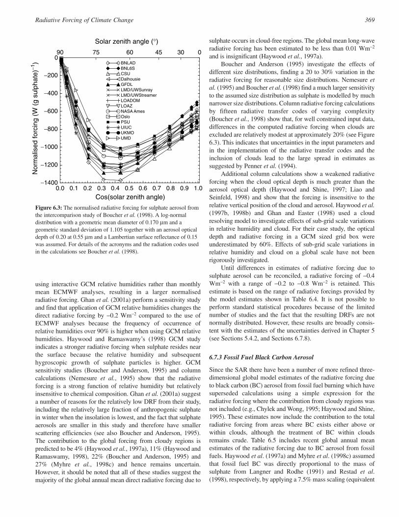
using interactive GCM relative humidities rather than monthlymean ECMWF analyses, resulting in a larger normalisedradiative forcing. Ghan et al. (2001a) perform a sensitivity studyand find that application of GCM relative humidities changes thedirect radiative forcing by −0.2 Wm−2 compared to the use ofECMWF analyses because the frequency of occurrence ofrelative humidities over 90% is higher when using GCM relativehumidities. Haywood and Ramaswamy’s (1998) GCM studyindicates a stronger radiative forcing when sulphate resides nearthe surface because the relative humidity and subsequenthygroscopic growth of sulphate particles is higher. GCMsensitivity studies (Boucher and Anderson, 1995) and columncalculations (Nemesure et al., 1995) show that the radiativeforcing is a strong function of relative humidity but relativelyinsensitive to chemical composition. Ghan et al. (2001a) suggesta number of reasons for the relatively low DRF from their study,including the relatively large fraction of anthropogenic sulphatein winter when the insolation is lowest, and the fact that sulphateaerosols are smaller in this study and therefore have smallerscattering efficiencies (see also Boucher and Anderson, 1995).The contribution to the global forcing from cloudy regions ispredicted to be 4% (Haywood et al., 1997a), 11% (Haywood andRamaswamy, 1998), 22% (Boucher and Anderson, 1995) and27% (Myhre et al., 1998c) and hence remains uncertain.However, it should be noted that all of these studies suggest themajority of the global annual mean direct radiative forcing due to
sulphate occurs in cloud-free regions. The global mean long-waveradiative forcing has been estimated to be less than 0.01 Wm−2
and is insignificant (Haywood et al., 1997a).Boucher and Anderson (1995) investigate the effects of
different size distributions, finding a 20 to 30% variation in theradiative forcing for reasonable size distributions. Nemesure etal. (1995) and Boucher et al. (1998) find a much larger sensitivityto the assumed size distribution as sulphate is modelled by muchnarrower size distributions. Column radiative forcing calculationsby fifteen radiative transfer codes of varying complexity(Boucher et al., 1998) show that, for well constrained input data,differences in the computed radiative forcing when clouds areexcluded are relatively modest at approximately 20% (see Figure6.3). This indicates that uncertainties in the input parameters andin the implementation of the radiative transfer codes and theinclusion of clouds lead to the large spread in estimates assuggested by Penner et al. (1994).
Additional column calculations show a weakened radiativeforcing when the cloud optical depth is much greater than theaerosol optical depth (Haywood and Shine, 1997; Liao andSeinfeld, 1998) and show that the forcing is insensitive to therelative vertical position of the cloud and aerosol. Haywood et al.(1997b, 1998b) and Ghan and Easter (1998) used a cloudresolving model to investigate effects of sub-grid scale variationsin relative humidity and cloud. For their case study, the opticaldepth and radiative forcing in a GCM sized grid box wereunderestimated by 60%. Effects of sub-grid scale variations inrelative humidity and cloud on a global scale have not beenrigorously investigated.
Until differences in estimates of radiative forcing due tosulphate aerosol can be reconciled, a radiative forcing of −0.4Wm−2 with a range of −0.2 to −0.8 Wm−2 is retained. Thisestimate is based on the range of radiative forcings provided bythe model estimates shown in Table 6.4. It is not possible toperform standard statistical procedures because of the limitednumber of studies and the fact that the resulting DRFs are notnormally distributed. However, these results are broadly consis-tent with the estimates of the uncertainties derived in Chapter 5(see Sections 5.4.2, and Sections 6.7.8).
6.7.3 Fossil Fuel Black Carbon Aerosol
Since the SAR there have been a number of more refined three-dimensional global model estimates of the radiative forcing dueto black carbon (BC) aerosol from fossil fuel burning which havesuperseded calculations using a simple expression for theradiative forcing where the contribution from cloudy regions wasnot included (e.g., Chylek and Wong, 1995; Haywood and Shine,1995). These estimates now include the contribution to the totalradiative forcing from areas where BC exists either above orwithin clouds, although the treatment of BC within cloudsremains crude. Table 6.5 includes recent global annual meanestimates of the radiative forcing due to BC aerosol from fossilfuels. Haywood et al. (1997a) and Myhre et al. (1998c) assumedthat fossil fuel BC was directly proportional to the mass ofsulphate from Langner and Rodhe (1991) and Restad et al.(1998), respectively, by applying a 7.5% mass scaling (equivalent
369Radiative Forcing of Climate Change
0.0 0.1 0.2 0.3 0.4 0.5 0.6 0.7 0.8 0.9 1.0
Cos(solar zenith angle)
−1400
−1200
−1000
−800
−600
−400
−200
0
Nor
mal
ised
forc
ing
(W (
g su
lpha
te)−1
) BNLADBNL6SCSUDalhousieGFDLLMD/UWSunrayLMD/UWStreamerLOADOMLOAZNASA AmesOsloPSUUIUCUKMOUMD
90 75 60 45 30 0
Solar zenith angle (°)
Figure 6.3: The normalised radiative forcing for sulphate aerosol fromthe intercomparison study of Boucher et al. (1998). A log-normaldistribution with a geometric mean diameter of 0.170 µm and ageometric standard deviation of 1.105 together with an aerosol opticaldepth of 0.20 at 0.55 µm and a Lambertian surface reflectance of 0.15was assumed. For details of the acronyms and the radiation codes usedin the calculations see Boucher et al. (1998).
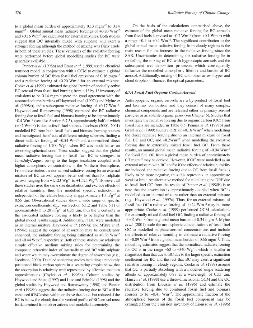
to a global mean burden of approximately 0.13 mgm−2 to 0.14mgm−2). Global annual mean radiative forcings of +0.20 Wm−2
and +0.16 Wm−2 are calculated for external mixtures. Both studiessuggest that BC internally mixed with sulphate will exert astronger forcing although the method of mixing was fairly crudein both of these studies. These estimates of the radiative forcingwere performed before global modelling studies for BC weregenerally available.
Penner et al. (1998b) and Grant et al. (1999) used a chemicaltransport model in conjunction with a GCM to estimate a globalcolumn burden of BC from fossil fuel emissions of 0.16 mgm−2
and a radiative forcing of +0.20 Wm−2 for an external mixture.Cooke et al. (1999) estimated the global burden of optically activeBC aerosol from fossil fuel burning from a 1° by 1° inventory ofemissions to be 0.14 mgm−2 (note the good agreement with theassumed column burdens of Haywood et al. (1997a) and Myhre etal. (1998c)) and a subsequent radiative forcing of +0.17 Wm−2.Haywood and Ramaswamy (1998) estimated the BC radiativeforcing due to fossil fuel and biomass burning to be approximately+0.4 Wm−2 (see also Section 6.7.5), approximately half of which(+0.2 Wm−2) is due to fossil fuel sources. Jacobson (2000, 2001)modelled BC from both fossil fuels and biomass burning sourcesand investigated the effects of different mixing schemes, finding adirect radiative forcing of +0.54 Wm−2 and a normalised directradiative forcing of 1,200 Wg−1 when BC was modelled as anabsorbing spherical core. These studies suggest that the globalmean radiative forcing due to fossil fuel BC is strongest inJune/July/August owing to the larger insolation coupled withhigher atmospheric concentrations in the Northern Hemisphere.From these studies the normalised radiative forcing for an externalmixture of BC aerosol appears better defined than for sulphateaerosol ranging from +1,123 Wg−1 to +1,525 Wg−1. However, allthese studies used the same size distribution and exclude effects ofrelative humidity, thus the modelled specific extinction isindependent of the relative humidity at approximately 10 m2g−1 at0.55 µm. Observational studies show a wide range of specificextinction coefficients, αsp, (see Section 5.1.2 and Table 5.1) ofapproximately 5 to 20 m2g−1 at 0.55 µm, thus the uncertainty inthe associated radiative forcing is likely to be higher than theglobal model results suggest. Additionally, if BC were modelledas an internal mixture, Haywood et al. (1997a) and Myhre et al.(1998c) suggest the degree of absorption may be considerablyenhanced, the radiative forcing being estimated as +0.36 Wm−2
and +0.44 Wm−2, respectively. Both of these studies use relativelysimple effective medium mixing rules for determining thecomposite refractive index of internally mixed BC with sulphateand water which may overestimate the degree of absorption (e.g.,Jacobson, 2000). Detailed scattering studies including a randomlypositioned black carbon sphere in a scattering droplet show thatthe absorption is relatively well represented by effective mediumapproximations (Chylek et al., 1996b). Column studies byHaywood and Shine (1997) and Liao and Seinfeld (1998) and theglobal studies by Haywood and Ramaswamy (1998) and Penneret al. (1998b) suggest that the radiative forcing due to BC will beenhanced if BC exists within or above the cloud, but reduced if theBC is below the cloud; thus the vertical profile of BC aerosol mustbe determined from observations and modelled accurately.
On the basis of the calculations summarised above, theestimate of the global mean radiative forcing for BC aerosolsfrom fossil fuels is revised to +0.2 Wm−2 (from +0.1 Wm−2) witha range +0.1 to +0.4 Wm−2. The significant contribution to theglobal annual mean radiative forcing from cloudy regions is themain reason for the increase in the radiative forcing since theSAR. Uncertainties in determining the radiative forcing lie inmodelling the mixing of BC with hygroscopic aerosols and thesubsequent wet deposition processes which consequentlyinfluence the modelled atmospheric lifetime and burden of BCaerosol. Additionally, mixing of BC with other aerosol types andcloud droplets influences the optical parameters.
6.7.4 Fossil Fuel Organic Carbon Aerosol
Anthropogenic organic aerosols are a by-product of fossil fueland biomass combustion and they consist of many complexchemical compounds and are released either as primary aerosolparticles or as volatile organic gases (see Chapter 5). Studies thatinvestigate the radiative forcing due to organic carbon (OC) fromfossil fuels are included in Table 6.5. Penner et al. (1998b) andGrant et al. (1999) found a DRF of +0.16 Wm−2 when modellingthe direct radiative forcing due to an internal mixture of fossilfuel BC and OC, and +0.2Wm−2 when modelling the radiativeforcing due to externally mixed fossil fuel BC. From theseresults, an annual global mean radiative forcing of −0.04 Wm−2
for fossil fuel OC from a global mean burden of approximately0.7 mgm−2 may be derived. However, if OC were modelled as anexternal mixture with BC and/or if the effects of relative humidityare included, the radiative forcing due to OC from fossil fuels islikely to be more negative, thus this represents an approximateweakest limit. An alternative method for calculating the DRF dueto fossil fuel OC from the results of Penner et al. (1998b) is tonote that the absorption is approximately doubled when BC ismodelled as an internal mixture rather than an external mixture(e.g., Haywood et al., 1997a). Thus, for an external mixture offossil fuel OC a radiative forcing of –0.24 Wm−2 may be moreappropriate. Cooke et al. (1999) performed GCM calculationsfor externally mixed fossil fuel OC, finding a radiative forcing of−0.02 Wm−2 from a global mean burden of 0.34 mgm−2. Myhreet al. (2001) scale the atmospheric concentrations of fossil fuelOC to modelled sulphate aerosol concentrations and includethe effects of relative humidity to estimate a radiative forcingof −0.09 Wm−2 from a global mean burden of 0.66 mgm−2. Thus,modelling estimates suggest that the normalised radiative forcingfor OC is in the range −60 to −340 Wg−1, which is smaller inmagnitude than that due to BC due to the larger specific extinctioncoefficient for BC and the fact that BC may exert a significantradiative forcing in cloudy regions. Cooke et al. (1999) assumethat OC is partially absorbing with a modelled single scatteringalbedo of approximately 0.97 at a wavelength of 0.55 µm.Hansen et al. (1998) use a three-dimensional GCM and the OCdistribution from Liousse et al. (1996) and estimate theradiative forcing due to combined fossil fuel and biomasssources to be −0.41 Wm−2. The approximate fraction of theatmospheric burden of the fossil fuel component may beestimated from the emission inventory of Liousse et al. (1996)
370 Radiative Forcing of Climate Change
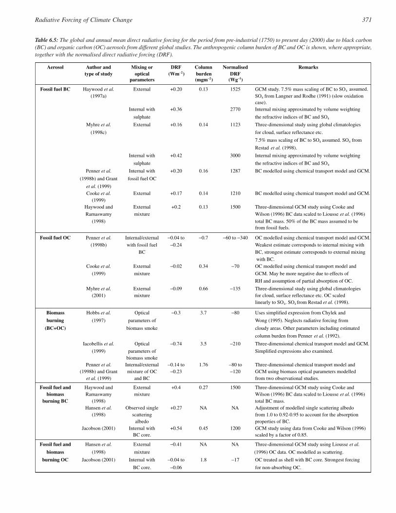
371Radiative Forcing of Climate Change
Aerosol Author andtype of study
Mixing oroptical
parameters
DRF(Wm−2)
Columnburden(mgm−2)
NormalisedDRF
(Wg−1)
Remarks
Fossil fuel BC Haywood et al.(1997a)
External +0.20 0.13 1525 GCM study. 7.5% mass scaling of BC to SO4
SO4 from Langner and Rodhe (1991) (slow oxidation case).
Internal with
sulphate
+0.36 2770 Internal mixing approximated by volume weighting
the refractive indices of BC and SO4
Myhre et al.
(1998c)
External +0.16 0.14 1123 Three-dimensional study using global climatologies
for cloud, surface reflectance etc.
7.5% mass scaling of BC to SO4 assumed. SO4
Restad et al. (1998).
Internal with
sulphate
+0.42 3000 Internal mixing approximated by volume weighting
the refractive indices of BC and SO4
Penner et al.
(1998b) and Grant
et al. (1999)
Internal with
fossil fuel OC
+0.20 0.16 1287 BC modelled using chemical transport model and GCM.
Cooke et al.(1999)
External +0.17 0.14 1210 BC modelled using chemical transport model and GCM.
Haywood and
Ramaswamy
(1998)
External
mixture
+0.2 0.13 1500 Three-dimensional GCM study using Cooke and
Wilson (1996) BC data scaled to Liousse et al. (1996)
total BC mass. 50% of the BC mass assumed to be from fossil fuels.
Fossil fuel OC Penner et al.
(1998b)
Internal/external
with fossil fuel
BC
−0.04 to
−0.24
−0.7 −60 to −340 OC modelled using chemical transport model and GCM.
Weakest estimate corresponds to internal mixing with
BC, strongest estimate corresponds to external mixing
with BC.Cooke et al.
(1999)
External
mixture
−0.02 0.34 −70 OC modelled using chemical transport model and
GCM. May be more negative due to effects of
RH and assumption of partial absorption of OC.
Myhre et al.(2001)
Externalmixture
−0.09 0.66 −135 Three-dimensional study using global climatologies for cloud, surface reflectance etc. OC scaled linearly to SO4. SO4 from Restad et al. (1998).
Biomass
burning
(BC+OC)
Hobbs et al.
(1997)
Optical
parameters of
biomass smoke
−0.3 3.7 −80 Uses simplified expression from Chylek and
Wong (1995). Neglects radiative forcing from
cloudy areas. Other parameters including estimated
column burden from Penner et al. (1992).
Iacobellis et al.
(1999)
Optical
parameters ofbiomass smoke
−0.74 3.5 −210 Three-dimensional chemical transport model and GCM.
Simplified expressions also examined.
Penner et al.(1998b) and Grant
et al. (1999)
Internal/externalmixture of OC
and BC
−0.14 to−0.23
1.76 −80 to−120
Three-dimensional chemical transport model andGCM using biomass optical parameters modelledfrom two observational studies.
Fossil fuel andbiomass
burning BC
Haywood andRamaswamy
(1998)
Externalmixture
+0.4 0.27 1500 Three-dimensional GCM study using Cooke andWilson (1996) BC data scaled to Liousse et al. (1996) total BC mass.
Hansen et al.(1998)
Observed singlescattering
albedo
+0.27 NA NA Adjustment of modelled single scattering albedofrom 1.0 to 0.92-0.95 to account for the absorption properties of BC.
Jacobson (2001) Internal withBC core.
+0.54 0.45 1200 GCM study using data from Cooke and Wilson (1996) scaled by a factor of 0.85.
Fossil fuel and
biomass
burning OC
Hansen et al.
(1998)
External
mixture
−0.41 NA NA Three-dimensional GCM study using Liousse et al.
(1996) OC data. OC modelled as scattering.
Jacobson (2001) Internal with
BC core.
−0.04 to
−0.06
1.8 −17 OC treated as shell with BC core. Strongest forcing
for non-absorbing OC.
from
assumed.
Table 6.5: The global and annual mean direct radiative forcing for the period from pre-industrial (1750) to present day (2000) due to black carbon(BC) and organic carbon (OC) aerosols from different global studies. The anthropogenic column burden of BC and OC is shown, where appropriate,together with the normalised direct radiative forcing (DRF).
who estimate that fossil fuels contribute 38% to the total OCemissions. Thus the radiative forcing due to fossil fuel OC maybe inferred to be approximately −0.16 Wm−2. This may constitutean approximate upper estimate as the majority of fossil fuel OCoccurs over mid-latitude land areas where the surface reflectanceis generally higher and insolation is lower than in the equatorialregions where biomass burning is the major source of OC. Fromthese calculations, the radiative forcing due to fossil fuel OC isestimated to be −0.10 Wm−2. The uncertainty associated with thisestimate is necessarily high due to the limited number of detailedstudies and is estimated to be at least a factor of three.
6.7.5 Biomass Burning Aerosol
Biomass burning aerosol consists of two major chemicalcomponents: black carbon (BC), which primarily absorbs solarradiation, and organic carbon (OC), which primarily scatterssolar radiation. Sources of biomass burning aerosol includeburning of forests and savanna for colonisation and agriculture,burning of agricultural waste, and substances burned for fuelsuch as wood, dung and peat. Not all biomass aerosol comesfrom anthropogenic activities, as naturally occurring vegetationfires regularly occur. The fraction of anthropogenic biomassaerosol remains difficult to deduce. As for sulphate and fossilfuel BC aerosol, three-dimensional GCM estimates (e.g., Penneret al., 1998b) have superseded earlier simple box-model calcula-tions (e.g., Penner et al., 1992) (see Table 6.5). Penner et al.(1998b) and Grant et al. (1999) used a GCM to model theradiative forcing from biomass aerosol, finding a combined totalradiative forcing of −0.14 to −0.23 Wm−2 depending upon themixing assumptions and size distributions used. The radiativeforcing is calculated to be negative over the majority of theglobe, but some limited areas of positive forcing exist over areaswith a high surface reflectance (see Section 6.14.2). Theseasonal cycle is strongly influenced by the seasonal cycle ofbiomass burning emissions (Grant et al., 1999; Iacobellis et al.,1999), the global mean being estimated to be a maximum duringJune/July/August. Hobbs et al. (1997) performed aircraftmeasurements of smoke from biomass burning during theSmoke Cloud and Radiation-Brazil (SCAR-B) experiment andused the model of Penner et al. (1992) to estimate a global meanradiative forcing of −0.3 Wm−2 as an approximate upper limitdue to modified optical parameters. Ross et al. (1998) performeda similar measurement and modelling study estimating a localannual mean radiative forcing of −2 to −3 Wm−2 in intensivebiomass burning regions, indicating that the global meanradiative forcing is likely to be significantly smaller than inPenner et al. (1992). Iacobellis et al. (1999) model the globalradiative forcing as −0.7 Wm−2 but use an emission factor forbiomass aerosols that Liousse et al. (1996) suggest is a factor ofthree too high, thus a radiative forcing of −0.25 Wm−2 is morelikely. These estimates neglect any long-wave radiative forcingalthough Christopher et al. (1996) found a discernible signal inAVHRR data from Brazilian forest fires that opposes the short-wave radiative forcing; the magnitude of the long-wave signalwill depend upon the size, optical parameters, and altitude of theaerosol.
The radiative effects of the individual BC and OCcomponents from biomass burning have also received attention.Haywood and Ramaswamy (1998) re-scaled the global columnburden of BC from Cooke and Wilson (1996) to that of Liousseet al. (1996) which is thought to be more representative ofoptically active BC and estimated the radiative forcing due tofossil fuel and biomass burning to be approximately +0.4 Wm−2,approximately half of which, or +0.2 Wm−2, is due to biomasssources. Hansen et al. (1998) adjusted the single scatteringalbedo of background aerosols from unity to 0.92 to 0.95 toaccount for the absorbing properties of BC from combined fossilfuel and biomass emissions and found a radiative forcing of+0.27 Wm−2.
The radiative forcing due to the purely scattering OCcomponent from combined fossil fuel and biomass emissions isestimated by Hansen et al. (1998) to be −0.41 Wm−2 with aapproximate upper limit for the radiative forcing due to fossil fuelOC from this study of approximately −0.16 Wm−2 (see Section6.7.4). Thus an approximate weakest limit for the radiativeforcing due to biomass burning OC is −0.25 Wm−2. Jacobson(2001) used a multi-component aerosol model to investigate theradiative forcing due to OC from combined fossil fuel andbiomass aerosols using emissions from Liousse et al. (1996)finding a resultant radiative forcing of between –0.04 and –0.06Wm−2, the strongest forcing being for purely scattering aerosol.The small radiative forcings of Jacobson (2001) may be due tothe aerosol being modelled as tri-modal with less aerosol in theoptically active region of the spectrum, or due to the fact thatabsorption by BC may be enhanced in the modelled multi-component mixture.
On the basis of these studies, the estimate of the radiativeforcing due to biomass burning aerosols remains the same at −0.2Wm−2. The uncertainty associated with the radiative forcing isvery difficult to estimate due to the limited number of studiesavailable and is estimated as at least a factor of three, leading toa range of –0.07 to –0.6 Wm−2.
6.7.6 Mineral Dust Aerosol
Recent studies have suggested that 20% (Sokolik and Toon,1996) and up to 30 to 50% (Tegen and Fung, 1995) of the totalmineral dust in the atmosphere originates from anthropogenicactivities, the precise fraction of mineral dust of anthropogenicorigin being extremely difficult to determine. Only the radiativeforcing from this anthropogenic component is considered as thereis no evidence that the naturally occurring component haschanged since 1750, although ice core measurements suggest thatatmospheric concentrations of dust have varied substantially overlonger time-scales (e.g., Petit, 1990). Because mineral dustparticles are of a relatively large size and because it becomeslofted to high altitudes in the troposphere, in addition to the short-wave radiative forcing, it may exert a significant long-waveradiative forcing. The global mean short-wave radiative forcingwill be negative due to the predominantly scattering nature in thesolar spectrum (although partial absorption may lead to a localpositive radiative forcing over high surface albedos and clouds)and the global mean long-wave forcing will be positive.
372 Radiative Forcing of Climate Change
Sokolik and Toon (1996) used a simple box model andneglected forcing in cloudy regions to estimate a short-waveradiative forcing of −0.25 Wm−2 over ocean and −0.6 Wm−2 overland, leading to a global forcing of approximately −0.46 Wm−2.They point out that this is offset to some extent by a positive long-wave forcing. Tegen and Fung (1995) performed a more detailedthree-dimensional GCM modelling study of dust aerosol andestimated that approximately 30 to 50% of the total dust burdenis due to changes in land use associated with anthropogenicactivity. The radiative forcing using this data was estimated byTegen et al. (1996) to be −0.25 Wm−2 in the short-wave and +0.34Wm−2 in the long-wave, resulting in a net radiative forcing of+0.09 Wm−2. Updated calculations of the net radiative forcingbased on Miller and Tegen (1998) estimate the radiative forcingto be −0.22 Wm−2 in the short-wave and +0.16 Wm−2 in the long-wave, resulting in a net radiative forcing of −0.06 Wm−2. Hansenet al. (1998) perform similar calculations and calculate a netradiative forcing of −0.12 Wm−2 by assuming a different verticaldistribution, different optical parameters and using a differentglobal model. Jacobson (2001) used a multi-component globalaerosol model to estimate the direct radiative forcing to be –0.062Wm−2 in the short-wave and +0.05 Wm−2 in the long-wave,resulting in a net radiative forcing of –0.012 Wm−2. The effectsof non-sphericity of the mineral dust are not accounted for inthese calculations. Mishchenko et al. (1997) suggest that differ-ences in the optical parameters between model spheroids andactual dust particles do not exceed 10 to 15%, although changesof this magnitude may have a large effect on the radiative forcing(Miller and Tegen, 1998). An example of the geographical distri-bution of the radiative forcing is shown in Figure 6.7g (data fromTegen et al., 1996) which shows regions of positive and negativeforcing. Positive forcing tends to exist over regions of highsurface reflectance and negative radiative forcings tend to existover areas of low surface reflectance. This is due to the depend-ency of the forcing on surface reflectance and the additionaleffects of the long-wave radiative forcing.
One problem that needs to be solved is uncertainty inrepresentative refractive indices (Claquin et al., 1998), and howthey vary geographically due to different mineral compositionof different source regions (e.g., Lindberg et al., 1976). Sokoliket al. (1993) summarise the imaginary part of the refractiveindex for different geographic regions finding a range (−0.003ito approximately −0.02i) at a wavelength of 0.55 µm, anddifferences in refractive index in the long-wave from differentgeographical sources are also reported by Sokolik et al. (1998).Kaufman et al. (2001) use observations from the Landsatsatellite coupled with ground-based sun photometer measure-ments and suggest that Saharan dust has a smaller imaginaryrefractive index (−0.001i) at 0.55 µm and absorbs less solarradiation than that used in the above modelling studies leadingto a much enhanced shortwave radiative forcing. However, theincrease is much less in the modelling study of Hansen et al.(1998) who find the net radiative forcing changes from −0.12Wm−2 to −0.53 Wm−2 when dust is treated as conservativelyscattering. von Hoyningen-Huene et al. (1999) determine theimaginary part of the refractive index from surface basedabsorption and scattering measurements and find that a refrac-
tive index of −0.005i best fits the observations for Saharan dust,which is in agreement with the values reported by Sokolik et al.(1993). The refractive indices together with the assumed sizedistributions determine the optical parameters. The radiativeforcing is particularly sensitive to the single scattering albedo(Miller and Tegen, 1999). Additional uncertainties lie inmodelling the size distributions (Tegen and Lacis, 1996;Claquin et al., 1998) which, together with the refractive indices,determine the optical parameters. Measurements made by theAdvanced Very High Resolution Radiometer (AVHRR) byAckerman and Chung (1992), showed a local short-waveradiative perturbation off the west coast of Africa of −40 to−90 Wm−2 and a corresponding long-wave perturbation of +5to +20 Wm−2 at the top of the atmosphere. Relating instanta-neous observational measurements that do not account for theeffects of clouds, diurnal averaging of the radiation, theseasonal signal associated with emissions and the fraction ofmineral dust that is anthropogenic to the global mean radiativeforcing is very difficult. Because the resultant global mean netradiative forcing is a residual obtained by summing the short-wave and the long-wave radiative forcings which are of roughlycomparable magnitudes, the uncertainty in the radiative forcingis large and even the sign is in doubt due to the competing natureof the short-wave and long-wave effects. The studies abovesuggest, on balance, that the shortwave radiative forcing is likelyto be of a larger magnitude than the long-wave radiative forcing,which indicates that the net radiative forcing is likely to benegative, although a net positive radiative forcing cannot beruled out. Therefore a tentative range of −0.6 to +0.4 Wm−2 isadopted; a best estimate cannot be assigned as yet.
6.7.7 Nitrate Aerosol
Although IPCC (1994) identified nitrate aerosol as a significantanthropogenic source of aerosol, only three estimates of theradiative forcing are available. Van Dorland et al. (1997) hasproduced a very speculative radiative forcing estimate ofapproximately −0.03 Wm−2 for ammonium nitrate, whileAdams et al. (2001) derived a radiative forcing of −0.22 Wm−2
from an anthropogenic burden of 0.62 mg(NO3)m−2, andJacobson (2001) derived a radiative forcing of approximately–0.02 Wm−2 for a column burden of 0.7 mg(NO3)m−2. Itappears that the large discrepancy between the results ofJacobson (2001) and Adams et al. (2001) is that 90% of thenitrate is in the coarse mode in Jacobson (2001), which reducesthe scattering efficiency. Recent measurement studies byVeefkind et al. (1996) and ten Brink et al. (1997) in theNetherlands have shown that nitrate aerosol in the form ofammonium nitrate is a locally important aerosol species interms of aerosol mass in the optically active sub-micron sizerange and hence the associated radiative forcing. They alsoemphasise the problems in measuring the concentrations andsize distributions of nitrate which is a semi-volatile substance.The contradictory nature of the global studies means that no“best estimate” or range for the radiative forcing due to anthro-pogenic nitrate aerosol is presented in this report, though futurestudies may prove that it exerts a significant radiative forcing.
373Radiative Forcing of Climate Change
6.7.8 Discussion of Uncertainties
While the radiative forcing due to greenhouse gases may bedetermined to a reasonably high degree of accuracy (Section 6.3),the uncertainties relating to aerosol radiative forcings remain large,and rely to a large extent on the estimates from global modellingstudies that are difficult to verify at the present time. The range ofestimates presented in this section represents mainly the structuraluncertainties (i.e., differences in the model structures and assump-tions) rather than the parametric uncertainties (i.e., the uncertaintiesin the key parameters) (see Pan et al., 1997). This is because manyof the model calculations for sulphate aerosol use identical sizedistributions and refractive indices which lead to identical opticalparameters. Thus the model results are not necessarilyindependent, and certainly do not include the full range ofparametric uncertainties. The response of the direct radiativeforcing to parametric uncertainties is investigated in sensitivitystudies for different aerosol species (e.g., Boucher and Anderson,1995; Haywood and Ramaswamy, 1998). Three major areas ofuncertainty exist; uncertainties in the atmospheric burden and theanthropogenic contribution to it, uncertainties in the opticalparameters, and uncertainties in implementation of the opticalparameters and burden to give a radiative forcing. The atmosphericburden of an anthropogenic aerosol species is determined byfactors such as emission, aging, convective transport, scavengingand deposition processes, each of which have an associateduncertainty (see Chapter 5). The optical parameters have uncertain-ties associated with uncertainties in size distribution, chemicalcomposition, state of mixing, method of mixing, and asphericity.The problem of the degree of external/internal mixing in theatmosphere deserves highlighting, as global modelling studies tendto assume external mixtures which make modelling the sources,atmospheric transport and radiative properties simpler (e.g., Tegenet al., 1997). However, single particle analysis of particlescontaining mineral dust (e.g., Levin et al., 1996) and sea salt(Murphy et al., 1998) have often shown them to be internallymixed with sulphate and other aerosols of anthropogenic origin.Thus, heterogeneous conversion of SO2 to sulphate aerosol on dustor sea salt particles may effectively lead to sulphate becominginternally mixed with larger super-micron particles (e.g., Denteneret al., 1996) leading to a reduction in extinction efficiency, an effectthat has not yet been accounted for in global modelling studies.Studies that model internal mixtures of absorbing and scatteringaerosols necessarily apply simplifying assumptions such as volumeweighting the refractive indices (e.g., Haywood et al., 1997a;Myhre et al., 1998c) which may overestimate the degree of absorp-tion (e.g., Jacobson, 2000). Modelling studies that examine theeffects of internal mixing of multi-component aerosols are onlyjust becoming available (Jacobson, 2001). Uncertainties incalculating the radiative forcing from specified burdens and opticalparameters arise from uncertainties in the parametrization ofrelative humidity effects, the horizontal and vertical distributions ofthe aerosol, the uncertainties and sub-grid scale effects in othermodel fields such as clouds, humidity, temperature and surfacereflectance, the representation of the diurnal cycle, and theaccuracy of the radiation code used in the calculations. The shortatmospheric lifetime of aerosols and the resultant large spatial
variability imply a strong requirement for global observationaldata. Until a reliable global observational method for verifying theradiative effects of anthropogenic aerosols is available, it is likelythat the radiative forcing of any aerosol species will remain difficultto quantify. Although satellite retrievals of aerosol optical proper-ties have advanced substantially since the SAR, the difficultproblem of separating anthropogenic from natural aerosol stillremains (Chapter 5). Nevertheless, new analyses reiterate thatglobal satellite measurements contain tropospheric aerosolsignatures that include those due to anthropogenic aerosols(Haywood et al., 1999; Boucher and Tanré, 2000). While thegeneral spatial distribution of the radiative forcing for sulphateaerosol appears to be similar among the studies listed in Table 6.4,some important features, such as the seasonal cycle in the radiativeforcing, remain highly uncertain which may have importantconsequences in terms of the detection and attribution of climatechange (Chapter 12).
Here we examine the consistency of the ranges derived in thissection with the ranges obtained using the approach of Chapter 5,Section 5.4.2. For the industrial sulphate, fossil fuel BC, and fossilfuel OC aerosols, the “best estimates” of the direct radiative forcingare –0.4 Wm−2 with a factor of 2 uncertainty, +0.2 Wm−2 with afactor of 2 uncertainty and –0.1 Wm−2 with a factor of 3uncertainty, respectively. An estimate of the total direct radiativeforcing from industrial aerosols (using RMS errors) leads to arange –0.07 to –1.24 Wm−2 which is reasonably consistent with–0.1 to –1.0 Wm−2 (one standard deviation) from Chapter 5,Section 5.4.2. For biomass burning aerosols the “best estimate” ofthe direct radiative forcing is –0.2 Wm−2 with a range –0.07 to –0.6Wm−2, which is reasonably consistent with –0.1 to –0.5 Wm−2 (onestandard deviation) obtained from Section 5.4.2.
Additionally, while this section has concentrated upon theradiative forcing at the top of the atmosphere, the effects of anthro-pogenic aerosols upon the radiative budget at the surface of theEarth has not been considered in detail. For purely scatteringaerosols in cloud-free conditions, the radiative effect at the surfaceis within a few per cent of that at the top of the atmosphere (e.g.,Haywood and Shine, 1997). However, for partially absorbingaerosols, the radiative effect at the surface may be many times thatat the top of the atmosphere, as evidenced by modelling andmeasurement studies (e.g., Haywood and Shine, 1997; Haywood etal., 1999; Chapter 5). This is because, for partially absorbingaerosols, energy is transferred directly to the atmospheric column.Ackerman et al. (2000) point out that this can warm theatmosphere and “burn off” clouds. They conclude that during thenortheast monsoon (dry season over India) daytime trade cumuluscloud cover over the northern Indian Ocean can be reduced bynearly half, although these results depend strongly upon themeteorological conditions and modelling assumptions. Thisprocess may also be important over the global domain as indicatedby Hansen et al. (1997a), as the climate sensitivity parameter(Section 6.2) may differ significantly for absorbing aerosols due todiabatic heating in the aerosol layer modifying the temperaturestructure of the atmosphere, which affects the formation of clouds.The vertical partitioning of the forcing by absorbing aerosols isalso a potentially important factor in determining climatic changesat the surface (e.g., evaporation, soil moisture).
374 Radiative Forcing of Climate Change
6.8 The Indirect Radiative Forcing of Tropospheric Aerosols
6.8.1 Introduction
Aerosols serve as cloud condensation and ice nuclei, therebymodifying the microphysics, the radiative properties, and thelifetime of clouds. The physics and chemistry of the indirecteffect of aerosols is discussed in detail in Chapter 5. Onlyaspects directly relevant to quantifying the indirect radiativeforcing by aerosols are presented here. The aerosol indirecteffect is usually split into two effects: the first indirect effect,whereby an increase in aerosols causes an increase in dropletconcentration and a decrease in droplet size for fixed liquidwater content (Twomey, 1974), and the second indirect effect,whereby the reduction in cloud droplet size affects the precip-itation efficiency, tending to increase the liquid water content,the cloud lifetime (Albrecht, 1989), and the cloud thickness(Pincus and Baker, 1994). Until recently, the first indirecteffect has received much more attention than the second. IPCC(1994) and the SAR only considered the first indirect effect.Shine et al. (1996) retained a range of radiative forcing from 0to −1.5 Wm−2 with no best estimate, although a value of −0.8Wm−2 was used for the year 1990 in the IS92a scenario(Kattenberg et al., 1996). Here we review and discuss thevarious estimates for the globally averaged aerosol indirectforcing available in the literature. Because of the inherentcomplexity of the aerosol indirect effect, GCM studies dealingwith its quantification necessarily include an important level ofsimplification. While this represents a legitimate approach, itshould be clear that the GCM estimates of the aerosol indirecteffect are very uncertain. Section 6.8.2 investigates the indirectradiative forcing due to sulphate aerosols, on which mostefforts have concentrated, while other aerosol types are treatedin Section 6.8.3. Section 6.8.4 is devoted to alternativeapproaches, while Section 6.8.6 describes the aerosol indirecteffects on ice clouds.
6.8.2 Indirect Radiative Forcing by Sulphate Aerosols
6.8.2.1 Estimates of the first indirect effect The studies reported in Table 6.6 use different GCMs andmethods for computing the droplet number concentration(i.e., empirical relationships between the sulphate mass andthe cloud droplet number concentration, empirical relation-ships between the sulphate aerosol number concentration andthe cloud droplet number concentration, or parametrization ofcloud nucleation processes). The forcing estimates for thefirst indirect effect from sulphate aerosols range from −0.3 to−1.8 Wm−2, which is close to the range of 0 to −1.5 Wm−2
given in the SAR when only a few estimates were available.There is a tendency for more and more studies to use
interactive (on-line) rather than prescribed (monthly orannual mean) sulphate concentrations. Feichter et al. (1997)pointed out that the first indirect effect calculated frommonthly mean sulphate concentrations is 20% larger thancalculated from interactive sulphate concentrations. Jones etal. (1999) found that the total indirect effect was overesti-
mated by about 60% when they used seasonal or annual meansulphate concentrations.
The various GCM studies show some disagreement on thespatial distribution of the forcing, an example of which is shownin Figure 6.7h. The Northern to Southern Hemisphere ratio variesfrom 1.4 to 4 depending on the models. It is generally smallerthan the Northern to Southern Hemisphere ratio of anthropogenicsulphate aerosol concentrations because of the higher suscepti-bility of the clouds in the Southern Hemisphere (Platnick andTwomey, 1994; Taylor and McHaffie, 1994). The ocean to landratio depends very much on the method used to relate theconcentration of sulphate mass to the cloud droplet numberconcentration and on the natural background aerosol concentra-tions. It was generally found to be smaller than unity (Boucherand Lohmann, 1995; Jones and Slingo, 1997; Kiehl et al., 2000).Larger ratios, such as 1.6 (Chuang et al., 1997) and 5 (Jones andSlingo, 1997), are reported in some of the sensitivity experi-ments. Using a detailed inventory of ship sulphur emissions anda simple calculation of the aerosol indirect effect, Capaldo et al.(1999) suggested that a significant fraction of the effect over theoceans (−0.11 Wm−2, averaged globally) could be due to ship-emitted particulate matter (sulphate plus organic material). So farthis source of aerosols has not been included in the GCM studies.
Kogan et al. (1996, 1997) used the Warren et al. (1988)cloud climatology over the oceans rather than a GCM to predictthe indirect effect by sulphate aerosols on cloud albedo. Thecloud albedo susceptibility was evaluated from a large eddysimulation model applied to stratocumulus clouds. They found anindirect short-wave forcing of −1.1 Wm−2 over the oceans with asmall hemispheric difference of 0.4 Wm−2 (i.e., a Northern toSouthern Hemisphere ratio of about 1.4). In their study, theforcing had a strong seasonal cycle, with the SouthernHemisphere forcing prevailing in some seasons.
6.8.2.2 Estimates of the second indirect effect and of the combined effect
Whereas the first indirect effect can be computed diagnostically,assessment of the second indirect effect implies that twoindependent (i.e., with the same fixed sea surface temperatures,but with different meteorologies) GCM simulations be made, afirst one with pre-industrial and a second one with present dayaerosols. The difference in top of the atmosphere fluxes or cloudradiative forcings between two such simulations is used as aproxy for the forcings due to the second indirect and thecombined effects. The simulations need to be sufficiently long(usually 5 years) so that the effects of natural variability areexpected to average out. However, as a consequence, theestimates of the aerosol indirect effect may include some undesir-able feedbacks involving climate parameters which would violatethe definition adopted for radiative forcing of climate change byIPCC (see also Section 6.1.1). Rotstayn and Penner (2001)showed that, at least in their model, the difference in top of theatmosphere fluxes between two simulations did not differ bymore than 10% from the radiative forcing for the first indirecteffect computed diagnostically. Caution should nevertheless beexercised before this result can be generalised to other modelsand to the second indirect effect.
375Radiative Forcing of Climate Change
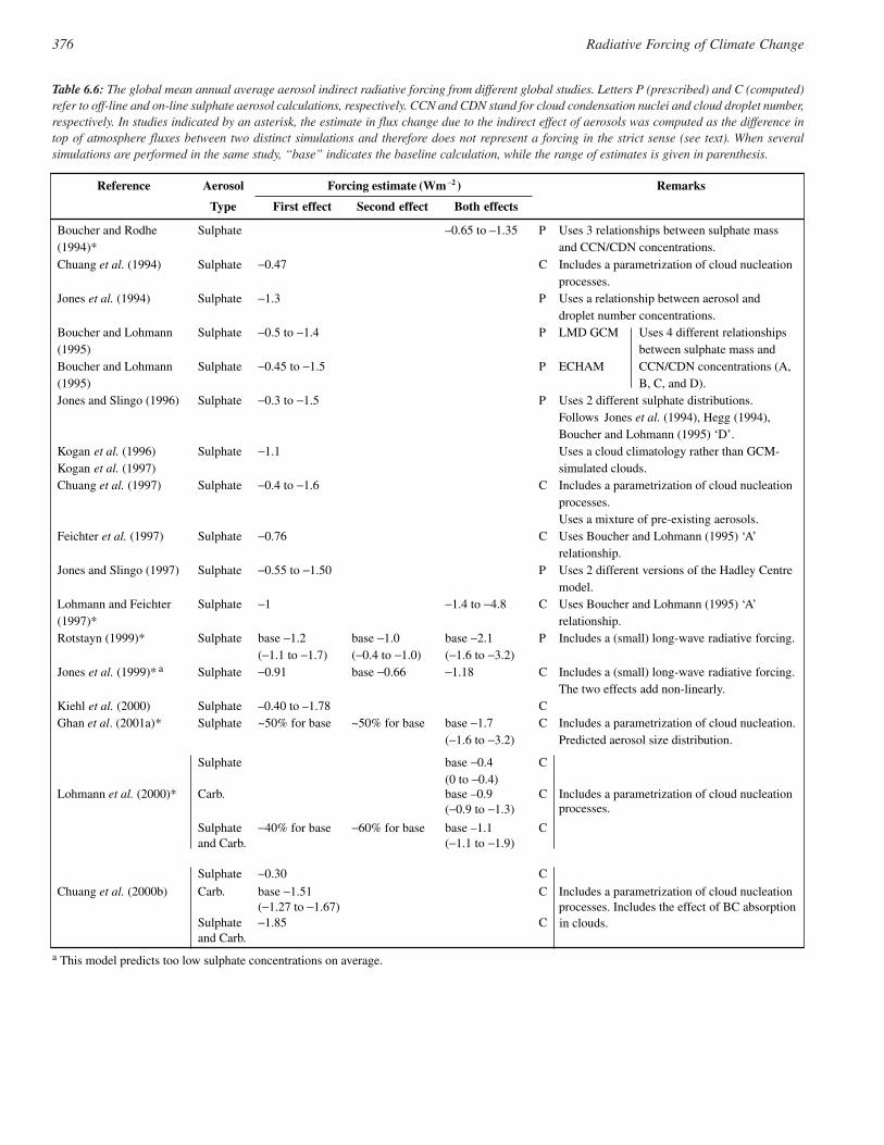
376 Radiative Forcing of Climate Change
Reference Aerosol Forcing estimate (Wm −2 ) Remarks
Type First effect Second effect Both effects
Boucher and Rodhe(1994)*
Sulphate –0.65 to –1.35 P Uses 3 relationships between sulphate massand CCN/CDN concentrations.
Chuang et al. (1994) Sulphate −0.47 C Includes a parametrization of cloud nucleationprocesses.
Jones et al. (1994) Sulphate −1.3 P Uses a relationship between aerosol anddroplet number concentrations.
Boucher and Lohmann(1995)
Sulphate −0.5 to −1.4 P LMD GCM Uses 4 different relationshipsbetween sulphate mass and
Boucher and Lohmann(1995)
Sulphate −0.45 to −1.5 P ECHAM CCN/CDN concentrations (A,B, C, and D).
Jones and Slingo (1996) Sulphate −0.3 to −1.5 P Uses 2 different sulphate distributions.Follows Jones et al. (1994), Hegg (1994),Boucher and Lohmann (1995) ‘D’.
Kogan et al. (1996)Kogan et al. (1997)
Sulphate −1.1 Uses a cloud climatology rather than GCM-simulated clouds.
Chuang et al. (1997) Sulphate −0.4 to −1.6 C Includes a parametrization of cloud nucleationprocesses.Uses a mixture of pre-existing aerosols.
Feichter et al. (1997) Sulphate −0.76 C Uses Boucher and Lohmann (1995) ‘A’relationship.
Jones and Slingo (1997) Sulphate −0.55 to −1.50 P Uses 2 different versions of the Hadley Centremodel.
Lohmann and Feichter(1997)*
Sulphate −1 −1.4 to −4.8 C Uses Boucher and Lohmann (1995) ‘A’relationship.
Rotstayn (1999)* Sulphate base −1.2(−1.1 to −1.7)
base −1.0(−0.4 to −1.0)
base −2.1(−1.6 to −3.2)
P Includes a (small) long-wave radiative forcing.
Jones et al. (1999)* a Sulphate −0.91 base −0.66 −1.18 C Includes a (small) long-wave radiative forcing.The two effects add non-linearly.
Kiehl et al. (2000) Sulphate –0.40 to –1.78 CGhan et al. (2001a) * Sulphate ~50% for base ~50% for base base −1.7
(−1.6 to −3.2)C Includes a parametrization of cloud nucleation.
Predicted aerosol size distribution.
Sulphate base −0.4(0 to −0.4)
C
Lohmann et al. (2000)* Carb. base –0.9(−0.9 to −1.3)
C Includes a parametrization of cloud nucleationprocesses.
Sulphateand Carb.
−40% for base −60% for base base –1.1(−1.1 to −1.9)
C
Sulphate −0.30 C
Chuang et al. (2000b) Carb. base −1.51(−1.27 to −1.67)
C Includes a parametrization of cloud nucleationprocesses. Includes the effect of BC absorption
Sulphateand Carb.
−1.85 C in clouds.
a This model predicts too low sulphate concentrations on average.
Table 6.6: The global mean annual average aerosol indirect radiative forcing from different global studies. Letters P (prescribed) and C (computed)refer to off-line and on-line sulphate aerosol calculations, respectively. CCN and CDN stand for cloud condensation nuclei and cloud droplet number,respectively. In studies indicated by an asterisk, the estimate in flux change due to the indirect effect of aerosols was computed as the difference intop of atmosphere fluxes between two distinct simulations and therefore does not represent a forcing in the strict sense (see text). When severalsimulations are performed in the same study, “base” indicates the baseline calculation, while the range of estimates is given in parenthesis.
Jones et al. (1999) and Rotstayn (1999) provide estimates forthe second indirect effect alone with ranges of −0.53 to −2.29Wm−2 and −0.4 to −1.0 Wm−2, respectively. For the combinedeffect (first and second effects estimated together), Jones et al.(1999) and Rotstayn (1999) give best estimates of −1.18 and −2.1Wm−2. Larger radiative impacts are found in sensitivity tests byRotstayn (1999) and Lohmann and Feichter (1997), with values of−3.2 and −4.8 Wm−2, respectively. Rotstayn (1999) tried analternative parametrization for cloud droplet concentration(Roelofs et al., 1998) and Lohmann and Feichter (1997) tried analternative cloud scheme. In contrast to these studies, Lohmann etal. (2000) adopted a “mechanistic” approach, where theyintroduced a prognostic equation for the cloud droplet numberconcentration. They predict a much smaller combined effect withradiative impact of 0.0 and −0.4 Wm−2, assuming externally andinternally mixed sulphate aerosols, respectively. The authorsattribute this rather small radiative impact to the small increase inanthropogenic sulphate aerosol number concentrations. Ghan etal. (2001a) estimate a combined effect of –1.7 Wm−2 using amechanistic approach similar to that of Lohmann et al., but withaerosol size distribution predicted rather than prescribed. Thelarger forcing is due to the absence of lower bounds on droplet andaerosol number concentrations in the simulations by Ghan et al.(2001a). Studies by Rotstayn (1999) and Jones et al. (1999) bothindicate that the positive long-wave forcing associated with theindirect aerosol effect is small (between 0.0 and 0.1 Wm−2 foreach of the effects).
The partitioning of the total indirect radiative impactbetween the first and second effect is uncertain. Jones et al.(1999) found that the ratio between their best estimates of the firstand second indirect effects, taken separately, was 1.38, whileLohmann et al. (2000) predicted a ratio of 0.71 (for sulphate andcarbonaceous aerosols taken together). Rotstayn (1999) andLohmann et al. (2000) estimated that the radiative impact for thecombined effects was of similar magnitude than the sum of thetwo effects considered separately. In contrast, Jones et al. (1999)found that the combined radiative impact (−1.18 Wm−2) was lessthan the sum of the two effects (estimated as −0.91 and −0.66Wm−2, respectively, yielding a sum of −1.57 Wm−2).
6.8.2.3 Further discussion of uncertaintiesSome authors have argued that sea salt particles may compete withsulphate aerosols as cloud condensation nuclei, thereby reducingthe importance of anthropogenic sulphate in droplet nucleation(Ghan et al., 1998; O’Dowd et al., 1999). While this process isempirically accounted for in some of the above mentionedestimates (e.g., Jones et al., 1999), it certainly adds furtheruncertainty to the estimates. Considerable sensitivity is found tothe parametrization of the autoconversion process (Boucher et al.,1995; Lohmann and Feichter, 1997; Delobbe and Gallée, 1998;Jones et al., 1999) which complicates matters because there is aneed to “tune” the autoconversion onset in GCMs (Boucher et al.,1995; Fowler et al., 1996; Rotstayn, 1999, 2000) to which theindirect aerosol forcing is sensitive (Jones et al., 1999; Rotstayn,1999; Ghan et al., 2001a). The indirect aerosol forcing is alsosensitive to the treatment of the pre-industrial aerosol concentrationand properties (Jones et al., 1999; Lohmann et al., 2000) which
remain poorly characterised, the representation of the microphysicsof mid-level clouds (Lohmann et al., 2000), the representation ofaerosol size distribution (Ghan et al., 2001a), the parametrizationof sub-grid scale clouds, the horizontal resolution of the GCM(Ghan et al., 2001a), and the ability of GCMs to simulate thestratocumulus cloud fields. Finally, it should be noted that all thestudies discussed above cannot be considered as truly“independent” because many of them (with the exceptions ofLohmann et al. (2000) and Ghan et al. (2001a)) use similarmethodologies and similar relationships between sulphate massand cloud droplet number concentration. Therefore it is suspectedthat the range of model results does not encompass the total rangeof uncertainties. In an overall sense, it can be concluded that theconsiderable sensitivities to the treatment of microphysical detailsassociated with aerosol-cloud interactions, and their linkages withmacroscopic cloud and circulation parameters, remain to bethoroughly explored.
6.8.3 Indirect Radiative Forcing by Other Species
6.8.3.1 Carbonaceous aerosolsIn this section, carbonaceous aerosols refer to the mixture (internalor external) of OC and BC aerosols. Carbonaceous aerosols (and inparticular biomass burning aerosols) are efficient cloud condensa-tion nuclei (see Chapter 5 and e.g., Novakov and Penner, 1993;Novakov and Corrigan, 1996). There have been few GCM studiesestimating the indirect forcing from carbonaceous aerosols. Penneret al. (1996) reported a range of forcing from −2.5 to −4.5 Wm−2
(not included in Table 6.6), which is probably an overestimatebecause of neglect of other aerosol types such as dust and sea saltand underestimated natural emissions of organic aerosols. In a newset of simulations using an updated model accounting for dust andsea salt aerosols, Chuang et al. (2000b) obtained a forcing of –1.51Wm−2 for the first indirect effect from carbonaceous aerosols(–0.52 and –1.16 Wm−2 for fossil fuel and biomass burningaerosols, respectively). This estimate includes the effect of blackcarbon absorption in cloud droplets. Lohmann et al. (2000)predicted a radiative impact for the combined effect (i.e., first andsecond effects) of −1.3 and −0.9 Wm−2 for externally and internallymixed carbonaceous aerosols, respectively. These estimates do notinclude the effects of secondary organic aerosols, nor the effects ofabsorption of solar radiation by black carbon within the cloud.
Kaufman and Nakajima (1993) used AVHRR data to analysebright warm clouds over Brazil during the biomass burning season.They found a decrease in the cloud reflectance when the smokeoptical thickness increased. Kaufman and Fraser (1997) used asimilar approach to observe thinner and less reflective clouds. Theyshowed that smoke from biomass burning aerosols reduced thecloud droplet size and increased the cloud reflectance for smokeoptical depth up to 0.8. They estimated the indirect radiativeforcing by smoke to be −2 Wm−2 over this region for the threemonths when biomass burning takes place, which would suggest amuch smaller global average. However, using a combination ofsatellite observations and a global chemistry model, Remer et al.(1999) estimated that 50% of the cumulative biomass burningaerosol indirect forcing occurs for smoke optical depth smallerthan 0.1, that is well away from the source regions.
377Radiative Forcing of Climate Change
6.8.3.2 Combination of sulphate and carbonaceous aerosolsLohmann et al. (2000) found that the radiative impact of sulphateand carbonaceous aerosols considered simultaneously (−1.5 and−1.1 Wm−2 for the externally and internally mixed assumptions,respectively) is comparable to the sum of the radiative impactscalculated separately (see Table 6.6). Chuang et al. (2000b)reached a similar conclusion in their experiments where theyconsidered only the first indirect effect, with a total radiativeforcing of –1.85 Wm−2. It is noteworthy, however, that in thesetwo studies, the predicted radiative forcings for sulphate aerosolsare on the low side. This indicates that it is not wise to add theradiative forcings due to sulphate and carbonaceous aerosolsobtained separately from two different models. In fact, most of theGCM studies of the indirect aerosol effect used sulphate as asurrogate for the total anthropogenic fraction of the aerosol (e.g.,Boucher and Lohmann, 1995; Feichter et al., 1997; Lohmann andFeichter, 1997). In this case the computed forcings incorporate theeffects of other aerosol types which have a similar spatial distri-bution to sulphate aerosols, such as nitrate aerosols or carbona-ceous aerosols from fossil fuel combustion. It will not include,however, the effects of biomass burning aerosols which have adifferent spatial distribution from sulphate aerosols.
Another issue is the potential for light-absorbing aerosols toincrease in-cloud absorption of solar radiation – and correspond-ingly decrease the cloud albedo – when incorporated inside clouddroplets. Twohy et al. (1989) concluded from measurements offthe coast of California and from simple radiative calculations thatthe observed levels of soot would not lead to a significant impacton the cloud albedo. Chylek et al. (1996a) estimated an upperbound for increased absorption of solar radiation of 1 to 3 Wm−2
(global and annual average) for a black carbon concentration of0.5 µgm−3. Considering the modelled atmospheric concentrationsof soot (Chapter 5 and Sections 6.7.3 and 6.7.5) and the fact thatonly a fraction of the soot is incorporated in the cloud droplets, theeffect is probably smaller by one to two orders of magnitude.Heintzenberg and Wendisch (1996) showed that the decrease inradiative forcing due to a decrease in soot concentrations withincreasing distances from the pollution sources could be compen-sated by a concurrent increase in the fraction of soot which isincorporated in the cloud droplets. Only one GCM study to datehas considered the in-cloud absorption of soot. Chuang et al.(2000b) estimated a radiative forcing for in-cloud BC of +0.07Wm−2 for the soot concentrations predicted by their model andusing an effective medium approximation. More studies areneeded to confirm these results.
6.8.3.3 Mineral dust aerosolsLevin et al. (1996) observed desert dust particles coated withsulphate. Such particles may originate from in-cloud scavengingof interstitial dust particles followed by evaporation of the clouddroplets, condensation of SO2 onto dust followed by oxidation, oreven coagulation of dust and sulphate particles. The presence ofsoluble material (which may be of anthropogenic origin) on thedesert dust particles converts them into large and effective CCNwhich may affect the cloud microphysics. Whether this effectresults in a significant climate forcing has not been investigatedand cannot presently be quantified.
6.8.3.4 Effect of gas-phase nitric acidKulmala et al. (1993, 1995, 1998) argued that enhanced concen-trations of condensable vapours (such as HNO3 and HCl) in theatmosphere could affect cloud properties by facilitating theactivation of cloud condensation nuclei. The impact of such aneffect on the planetary cloud albedo has not been assessed.
6.8.4 Indirect Methods for Estimating the Indirect Aerosol Effect
6.8.4.1 The “missing” climate forcingHansen and colleagues have used two alternative approaches tocharacterise and quantify any “missing” climate forcing besidesthat due to greenhouse gases, solar constant, O3, and aerosoldirect effect. Hansen et al. (1995) used a simplified GCM toinvestigate the impacts of various climate forcings on the diurnalcycle of surface air temperature and compared them withobservations. They found that, although the aerosol direct effector an increase in continental cloud albedo could contribute todamp the surface temperature diurnal cycle, only an increase incontinental cloud cover would be consistent with observations(Karl et al., 1993). The required cloud increase depends on cloudheight and would be of the order of 1% global coverage for lowclouds (i.e., 2 to 5% over land). We cannot rule out that such achange is an unidentified cloud feedback rather than a forcing.Hansen et al. (1997b) also argued that agreement betweenobserved and computed temperature trends requires the presenceof another forcing of at least −1 Wm−2 which is inferred as beingdue to the indirect effect. In their calculations, the direct tropo-spheric aerosol effect does not play a large net role, because themoderately absorbing aerosol assumption leads to an offsetbetween its sunlight reflecting and absorbing properties insofaras the top of the atmosphere irradiance change is concerned.However, this method assumes that the observed change intemperature since pre-industrial times is primarily a response toanthropogenic forcings, that all the other anthropogenic forcingsare well quantified, and that the climate sensitivity parameter(Section 6.1) predicted by the GCM is correct (Rodhe et al.,2000). Therefore it may simply be a coincidence that the estimateof Hansen et al. (1997b) is consistent with the GCM estimatesdiscussed above.
6.8.4.2 Remote sensing of the indirect effect of aerosolsHan et al. (1994) analysed AVHRR satellite radiances to retrievethe cloud droplet size of low-level clouds. They reported signifi-cant inter-hemispheric differences for both maritime andcontinental clouds. Boucher (1995) showed that, if this differenceis to be attributed to anthropogenic aerosols, it implies a differ-ential forcing of about −1 Wm−2 between the two hemispheres.Assuming a Northern Hemisphere to Southern Hemisphere ratioof 2:1 for the aerosol indirect effect, this would imply a globally-averaged forcing of −1.5 Wm−2. It is not clear, however, to whatextent changes in cloud droplet size are related to change inaerosol concentrations. For instance, Han et al. (1998) showedthat cloud albedo decreases with decreasing droplet size for theoptically thinner clouds over the oceans. While this does notinvalidate the aerosol indirect effect at all, it underlines the limita-
378 Radiative Forcing of Climate Change
tions in using satellite observed changes in droplet size tocompute the aerosol indirect forcing. Therefore it seems difficultat present to use satellite observations to estimate the first aerosolindirect forcing unless some changes in cloud albedo could betied to changes in aerosol concentrations under the assumption ofconstant liquid water content. Satellite observations do play,however, a key role for evaluating models of the indirect aerosolradiative effect (Ghan et al., 2001b).
6.8.5 Forcing Estimates for This Report
Shine and Forster (1999) proposed a value of the aerosol indirectforcing due to all aerosols of −1 Wm−2 with at least a factor oftwo uncertainty. Several observational studies (see Chapter 5)support the existence of the first aerosol indirect effect on low-level clouds and a negative sign for the associated radiativeforcing, but these studies do not give indications on what a(negative) upper bound of the forcing would be. GCM studiespredict radiative forcing for the first indirect effect of industrialaerosols in the range of –0.3 to –1.8 Wm−2. However, because ofthe uncertainties in the estimates discussed above, the limitedvalidation of GCM parametrizations and results, and because in-cloud absorption by black carbon aerosols was not considered inall but one of the GCM studies, we retain 0 Wm−2 as an upperbound for the first aerosol indirect effect. A lower bound of –2Wm−2 is selected on the basis of available GCM studies for thefirst indirect effect. Not too much emphasis should be given to theexact bounds of this interval because they do not carry any statis-tical meaning (Section 6.13.1) and because of the very low levelof scientific understanding associated to this forcing (see Section6.13.1 where this concept is defined).
Available GCM studies suggest that the radiative flux pertur-bations associated with the second effect could be of similarmagnitude to that of the first effect. There are no studies yet toconfirm unambiguously that the GCM estimates of the radiativeimpact associated with the second indirect effect can beinterpreted in the strict sense of a radiative forcing (see Sections6.1 and 6.8.2.2), and very few observations exist as yet to supportthe existence of a significant effect. Therefore we refrain fromgiving any estimate or range of estimates for the second aerosolindirect effect. However, this does not minimise the potentialimportance of this effect.
6.8.6 Aerosol Indirect Effect on Ice Clouds
6.8.6.1 Contrails and contrail-induced cloudinessUsing meteorological and air traffic data scaled to regionalobservations of contrail cover, Sausen et al. (1998) estimated thepresent day global mean cover by line-shaped contrails to beabout 0.1%. This results in a global and annual mean radiativeforcing by line-shaped contrails of 0.02 Wm−2 (Minnis et al.,1999), subject to uncertainties in the contrail cover, optical depth,ice particle size and shape (Meerkötter et al., 1999). We followFahey et al. (1999) and retain a range of 0.005 to 0.06 Wm−2 forthe present day forcing, around the best estimate of 0.02 Wm−2.
Contrails can evolve into extended cirrus clouds. Boucher(1999) and Fahey et al. (1999) have shown evidences that cirrus
occurrence and coverage may have increased in regions of highair traffic compared with the rest of the globe. Smith et al. (1998)reported the existence of nearly invisible layers of small icecrystals, which cause absorption of infrared radiation, and couldbe due to remnant contrail particles. From consideration of thespatial distribution of cirrus trends during the last 25 years, Faheyet al. (1999) gave a range of possible best estimates of 0 to 0.04Wm−2 for the radiative forcing due to aviation-induced cirrus.The available information on cirrus clouds was deemed insuffi-cient to determine a single best estimate or an uncertainty range.
6.8.6.2 Impact of anthropogenic aerosols on cirrus cloud microphysics
Measurements by Ström and Ohlsson (1998) in a region of highair traffic revealed higher crystal number concentrations in areasof the cloud affected by soot emissions from aircraft. If theobserved enhancement in crystal number density (which is abouta factor of 2) is associated with a reduction in the mean crystalsize, as confirmed by the measurements of Kristensson et al.(2000), a change in cloud radiative forcing may result. Wyser andStröm (1998) estimated the forcing, although very uncertain, tobe in the order of 0.3 Wm−2 in regions of dense air traffic underthe assumption of a 20% decrease of the mean crystal size. Noglobally averaged radiative forcing is available.
The sedimentation of ice particles from contrails mayremove water vapour from the upper troposphere. This effect isexpected to be more important in strongly supersaturated airwhen ice particles can fall without evaporating (Fahey et al.,1999). The impacts of such an effect on cirrus formation, verticalprofile of humidity and the subsequent radiative forcing have notbeen assessed.
Aerosols also serve as ice nuclei although it is wellrecognised that there are fewer ice nuclei than cloud condensa-tion nuclei. It is conceivable that anthropogenic aerosols emittedat the surface and transported to the upper troposphere affect theformation and properties of ice clouds. Jensen and Toon (1997)suggested that insoluble particles from the surface or sootparticles emitted by aircraft, if they serve as effective ice nuclei,can result in an increase in the cirrus cloud coverage. Laaksonenet al. (1997) argued that nitric acid pollution is able to cause anincrease in supercooled cirrus cloud droplet concentrations, andthereby influence climate (see Chapter 5, Section 5.3.6). Sucheffects, if significant at all, are not quantified at present.
6.9 Stratospheric Aerosols
IPCC (1992, 1994) and the SAR have dealt with the climaticeffects of episodic, explosive volcanic events which result insignificant enhancements of aerosol concentrations in the strato-sphere. The most dramatic of these in recent times has been the1991 eruption of Mt. Pinatubo. The radiative, chemical,dynamical and climatic consequences accompanying thetransient duration of sulphuric acid aerosols in the stratospherehave been discussed in previous IPCC assessments. The eruptionof Mt. Pinatubo reached a peak forcing of about −3 Wm−2
(uncertainty of 20%) in 1991 (Hansen et al., 1998; Stenchikov etal., 1998), and was plausibly the largest volcanic aerosol forcing
379Radiative Forcing of Climate Change
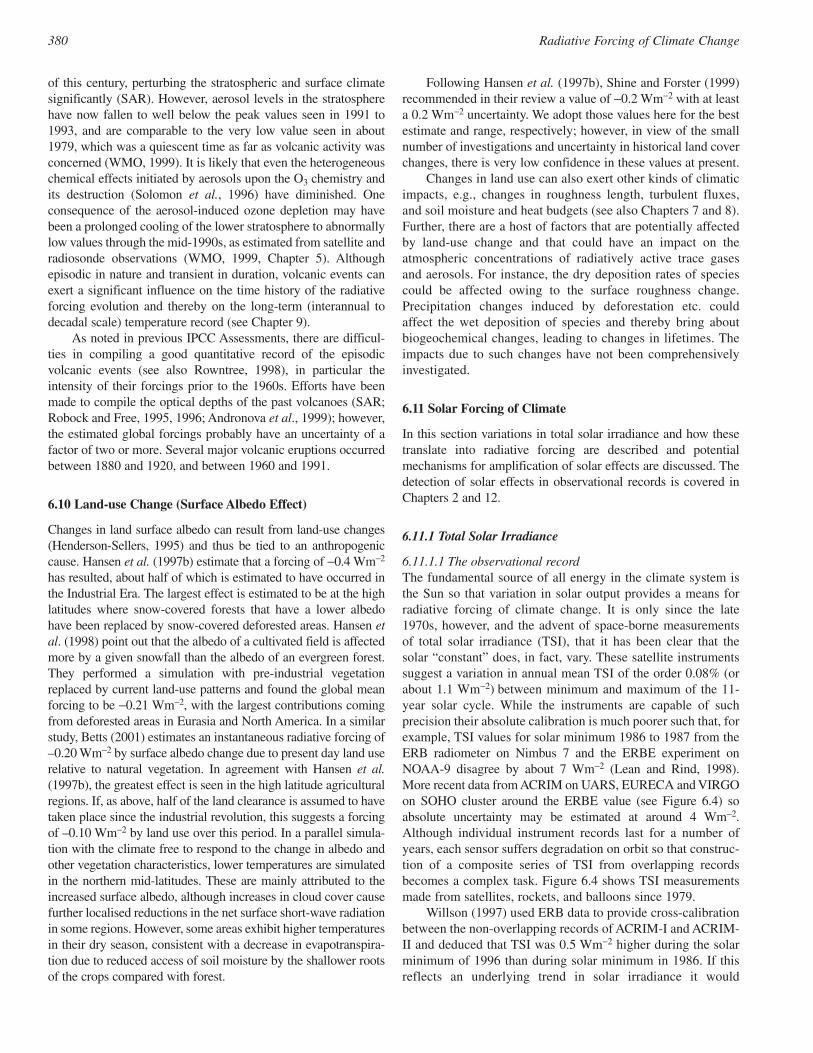
of this century, perturbing the stratospheric and surface climatesignificantly (SAR). However, aerosol levels in the stratospherehave now fallen to well below the peak values seen in 1991 to1993, and are comparable to the very low value seen in about1979, which was a quiescent time as far as volcanic activity wasconcerned (WMO, 1999). It is likely that even the heterogeneouschemical effects initiated by aerosols upon the O3 chemistry andits destruction (Solomon et al., 1996) have diminished. Oneconsequence of the aerosol-induced ozone depletion may havebeen a prolonged cooling of the lower stratosphere to abnormallylow values through the mid-1990s, as estimated from satellite andradiosonde observations (WMO, 1999, Chapter 5). Althoughepisodic in nature and transient in duration, volcanic events canexert a significant influence on the time history of the radiativeforcing evolution and thereby on the long-term (interannual todecadal scale) temperature record (see Chapter 9).
As noted in previous IPCC Assessments, there are difficul-ties in compiling a good quantitative record of the episodicvolcanic events (see also Rowntree, 1998), in particular theintensity of their forcings prior to the 1960s. Efforts have beenmade to compile the optical depths of the past volcanoes (SAR;Robock and Free, 1995, 1996; Andronova et al., 1999); however,the estimated global forcings probably have an uncertainty of afactor of two or more. Several major volcanic eruptions occurredbetween 1880 and 1920, and between 1960 and 1991.
6.10 Land-use Change (Surface Albedo Effect)
Changes in land surface albedo can result from land-use changes(Henderson-Sellers, 1995) and thus be tied to an anthropogeniccause. Hansen et al. (1997b) estimate that a forcing of −0.4 Wm−2
has resulted, about half of which is estimated to have occurred inthe Industrial Era. The largest effect is estimated to be at the highlatitudes where snow-covered forests that have a lower albedohave been replaced by snow-covered deforested areas. Hansen etal. (1998) point out that the albedo of a cultivated field is affectedmore by a given snowfall than the albedo of an evergreen forest.They performed a simulation with pre-industrial vegetationreplaced by current land-use patterns and found the global meanforcing to be −0.21 Wm−2, with the largest contributions comingfrom deforested areas in Eurasia and North America. In a similarstudy, Betts (2001) estimates an instantaneous radiative forcing of–0.20 Wm−2 by surface albedo change due to present day land userelative to natural vegetation. In agreement with Hansen et al.(1997b), the greatest effect is seen in the high latitude agriculturalregions. If, as above, half of the land clearance is assumed to havetaken place since the industrial revolution, this suggests a forcingof –0.10 Wm−2 by land use over this period. In a parallel simula-tion with the climate free to respond to the change in albedo andother vegetation characteristics, lower temperatures are simulatedin the northern mid-latitudes. These are mainly attributed to theincreased surface albedo, although increases in cloud cover causefurther localised reductions in the net surface short-wave radiationin some regions. However, some areas exhibit higher temperaturesin their dry season, consistent with a decrease in evapotranspira-tion due to reduced access of soil moisture by the shallower rootsof the crops compared with forest.
Following Hansen et al. (1997b), Shine and Forster (1999)recommended in their review a value of −0.2 Wm−2 with at leasta 0.2 Wm−2 uncertainty. We adopt those values here for the bestestimate and range, respectively; however, in view of the smallnumber of investigations and uncertainty in historical land coverchanges, there is very low confidence in these values at present.
Changes in land use can also exert other kinds of climaticimpacts, e.g., changes in roughness length, turbulent fluxes,and soil moisture and heat budgets (see also Chapters 7 and 8).Further, there are a host of factors that are potentially affectedby land-use change and that could have an impact on theatmospheric concentrations of radiatively active trace gasesand aerosols. For instance, the dry deposition rates of speciescould be affected owing to the surface roughness change.Precipitation changes induced by deforestation etc. couldaffect the wet deposition of species and thereby bring aboutbiogeochemical changes, leading to changes in lifetimes. Theimpacts due to such changes have not been comprehensivelyinvestigated.
6.11 Solar Forcing of Climate
In this section variations in total solar irradiance and how thesetranslate into radiative forcing are described and potentialmechanisms for amplification of solar effects are discussed. Thedetection of solar effects in observational records is covered inChapters 2 and 12.
6.11.1 Total Solar Irradiance
6.11.1.1 The observational recordThe fundamental source of all energy in the climate system isthe Sun so that variation in solar output provides a means forradiative forcing of climate change. It is only since the late1970s, however, and the advent of space-borne measurementsof total solar irradiance (TSI), that it has been clear that thesolar “constant” does, in fact, vary. These satellite instrumentssuggest a variation in annual mean TSI of the order 0.08% (orabout 1.1 Wm−2) between minimum and maximum of the 11-year solar cycle. While the instruments are capable of suchprecision their absolute calibration is much poorer such that, forexample, TSI values for solar minimum 1986 to 1987 from theERB radiometer on Nimbus 7 and the ERBE experiment onNOAA-9 disagree by about 7 Wm−2 (Lean and Rind, 1998).More recent data from ACRIM on UARS, EURECA and VIRGOon SOHO cluster around the ERBE value (see Figure 6.4) soabsolute uncertainty may be estimated at around 4 Wm−2.Although individual instrument records last for a number ofyears, each sensor suffers degradation on orbit so that construc-tion of a composite series of TSI from overlapping recordsbecomes a complex task. Figure 6.4 shows TSI measurementsmade from satellites, rockets, and balloons since 1979.
Willson (1997) used ERB data to provide cross-calibrationbetween the non-overlapping records of ACRIM-I and ACRIM-II and deduced that TSI was 0.5 Wm−2 higher during the solarminimum of 1996 than during solar minimum in 1986. If thisreflects an underlying trend in solar irradiance it would
380 Radiative Forcing of Climate Change
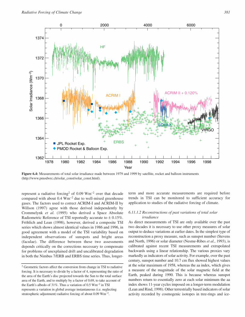
represent a radiative forcing2 of 0.09 Wm−2 over that decadecompared with about 0.4 Wm−2 due to well-mixed greenhousegases. The factors used to correct ACRIM-I and ACRIM-II byWillson (1997) agree with those derived independently byCrommelynk et al. (1995) who derived a Space AbsoluteRadiometric Reference of TSI reportedly accurate to ± 0.15%.Fröhlich and Lean (1998), however, derived a composite TSIseries which shows almost identical values in 1986 and 1996, ingood agreement with a model of the TSI variability based onindependent observations of sunspots and bright areas(faculae). The difference between these two assessmentsdepends critically on the corrections necessary to compensatefor problems of unexplained drift and uncalibrated degradationin both the Nimbus 7/ERB and ERBS time series. Thus, longer-
term and more accurate measurements are required beforetrends in TSI can be monitored to sufficient accuracy forapplication to studies of the radiative forcing of climate.
6.11.1.2 Reconstructions of past variations of total solar irradiance
As direct measurements of TSI are only available over the pasttwo decades it is necessary to use other proxy measures of solaroutput to deduce variations at earlier dates. In the simplest type ofreconstruction a proxy measure, such as sunspot number (Stevensand North, 1996) or solar diameter (Nesme-Ribes et al., 1993), iscalibrated against recent TSI measurements and extrapolatedbackwards using a linear relationship. The various proxies varymarkedly as indicators of solar activity. For example, over the pastcentury, sunspot number and 10.7 cm flux showed highest valuesat the solar maximum of 1958, whereas the aa index, which givesa measure of the magnitude of the solar magnetic field at theEarth, peaked during 1990. This is because whereas sunspotnumbers return to essentially zero at each solar minimum the aaindex shows 11-year cycles imposed on a longer-term modulation(Lean and Rind, 1998). Other terrestrially based indicators of solaractivity recorded by cosmogenic isotopes in tree-rings and ice-
381Radiative Forcing of Climate Change
1978 1980 1982 1984 1986 1988 1990 1992 1994 1996 1998 Year
1362
1364
1366
1368
1370
1372
1374
Sol
ar Ir
radi
ance
(W
m−2
)
0 2000 4000 6000
JPL Rocket Exp.PMOD Rocket & Balloon Exp.
HF
ACRIM I
ERBS
ACRIM II + 0.120%
SOVA2VIRGO
Figure 6.4: Measurements of total solar irradiance made between 1979 and 1999 by satellite, rocket and balloon instruments(http://www.pmodwrc.ch/solar_const/solar_const.html).
2 Geometric factors affect the conversion from change in TSI to radiativeforcing. It is necessary to divide by a factor of 4, representing the ratio ofthe area of the Earth’s disc projected towards the Sun to the total surfacearea of the Earth, and to multiply by a factor of 0.69, to take account ofthe Earth’s albedo of 31%. Thus a variation of 0.5 Wm−2 in TSIrepresents a variation in global average instantaneous (i.e. neglectingstratospheric adjustment) radiative forcing of about 0.09 Wm−2.
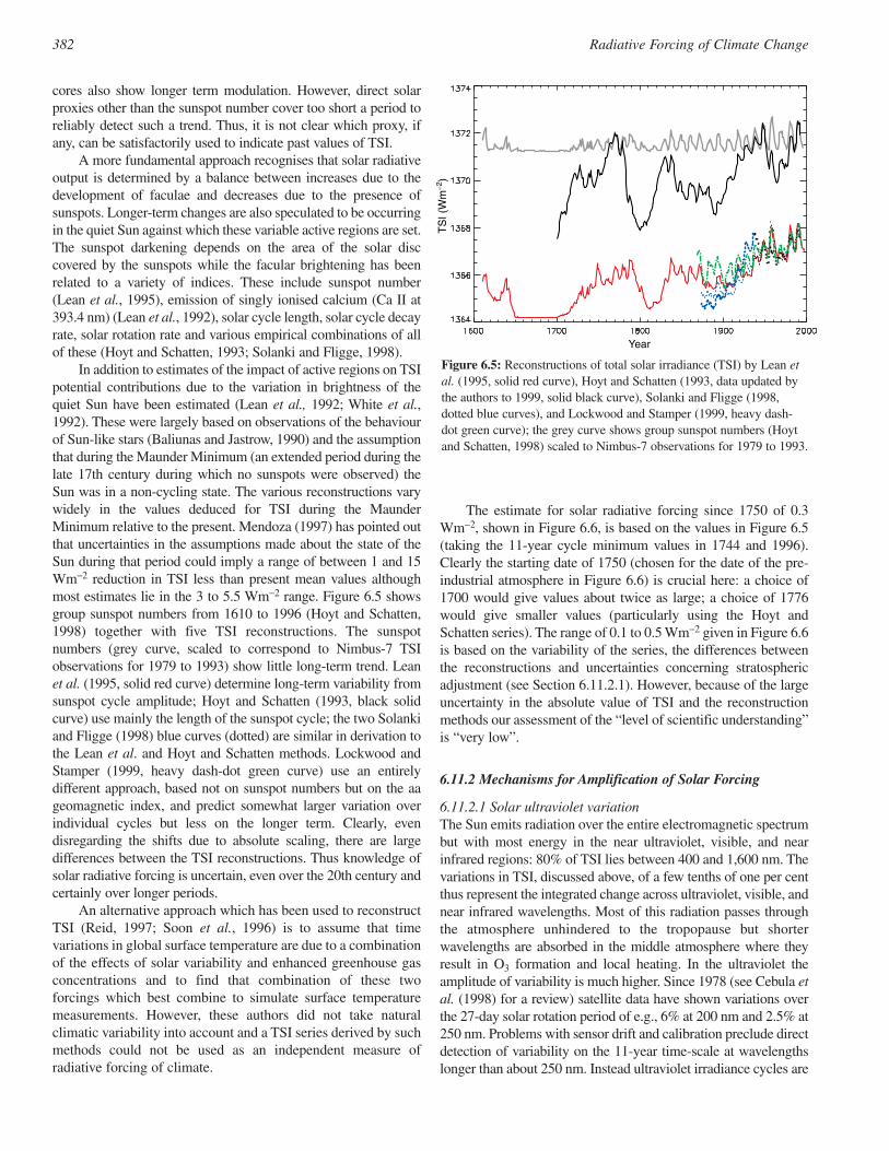
cores also show longer term modulation. However, direct solarproxies other than the sunspot number cover too short a period toreliably detect such a trend. Thus, it is not clear which proxy, ifany, can be satisfactorily used to indicate past values of TSI.
A more fundamental approach recognises that solar radiativeoutput is determined by a balance between increases due to thedevelopment of faculae and decreases due to the presence ofsunspots. Longer-term changes are also speculated to be occurringin the quiet Sun against which these variable active regions are set.The sunspot darkening depends on the area of the solar disccovered by the sunspots while the facular brightening has beenrelated to a variety of indices. These include sunspot number(Lean et al., 1995), emission of singly ionised calcium (Ca II at393.4 nm) (Lean et al., 1992), solar cycle length, solar cycle decayrate, solar rotation rate and various empirical combinations of allof these (Hoyt and Schatten, 1993; Solanki and Fligge, 1998).
In addition to estimates of the impact of active regions on TSIpotential contributions due to the variation in brightness of thequiet Sun have been estimated (Lean et al., 1992; White et al.,1992). These were largely based on observations of the behaviourof Sun-like stars (Baliunas and Jastrow, 1990) and the assumptionthat during the Maunder Minimum (an extended period during thelate 17th century during which no sunspots were observed) theSun was in a non-cycling state. The various reconstructions varywidely in the values deduced for TSI during the MaunderMinimum relative to the present. Mendoza (1997) has pointed outthat uncertainties in the assumptions made about the state of theSun during that period could imply a range of between 1 and 15Wm−2 reduction in TSI less than present mean values althoughmost estimates lie in the 3 to 5.5 Wm−2 range. Figure 6.5 showsgroup sunspot numbers from 1610 to 1996 (Hoyt and Schatten,1998) together with five TSI reconstructions. The sunspotnumbers (grey curve, scaled to correspond to Nimbus-7 TSIobservations for 1979 to 1993) show little long-term trend. Leanet al. (1995, solid red curve) determine long-term variability fromsunspot cycle amplitude; Hoyt and Schatten (1993, black solidcurve) use mainly the length of the sunspot cycle; the two Solankiand Fligge (1998) blue curves (dotted) are similar in derivation tothe Lean et al. and Hoyt and Schatten methods. Lockwood andStamper (1999, heavy dash-dot green curve) use an entirelydifferent approach, based not on sunspot numbers but on the aageomagnetic index, and predict somewhat larger variation overindividual cycles but less on the longer term. Clearly, evendisregarding the shifts due to absolute scaling, there are largedifferences between the TSI reconstructions. Thus knowledge ofsolar radiative forcing is uncertain, even over the 20th century andcertainly over longer periods.
An alternative approach which has been used to reconstructTSI (Reid, 1997; Soon et al., 1996) is to assume that timevariations in global surface temperature are due to a combinationof the effects of solar variability and enhanced greenhouse gasconcentrations and to find that combination of these twoforcings which best combine to simulate surface temperaturemeasurements. However, these authors did not take naturalclimatic variability into account and a TSI series derived by suchmethods could not be used as an independent measure ofradiative forcing of climate.
The estimate for solar radiative forcing since 1750 of 0.3Wm−2, shown in Figure 6.6, is based on the values in Figure 6.5(taking the 11-year cycle minimum values in 1744 and 1996).Clearly the starting date of 1750 (chosen for the date of the pre-industrial atmosphere in Figure 6.6) is crucial here: a choice of1700 would give values about twice as large; a choice of 1776would give smaller values (particularly using the Hoyt andSchatten series). The range of 0.1 to 0.5 Wm−2 given in Figure 6.6is based on the variability of the series, the differences betweenthe reconstructions and uncertainties concerning stratosphericadjustment (see Section 6.11.2.1). However, because of the largeuncertainty in the absolute value of TSI and the reconstructionmethods our assessment of the “level of scientific understanding”is “very low”.
6.11.2 Mechanisms for Amplification of Solar Forcing
6.11.2.1 Solar ultraviolet variationThe Sun emits radiation over the entire electromagnetic spectrumbut with most energy in the near ultraviolet, visible, and nearinfrared regions: 80% of TSI lies between 400 and 1,600 nm. Thevariations in TSI, discussed above, of a few tenths of one per centthus represent the integrated change across ultraviolet, visible, andnear infrared wavelengths. Most of this radiation passes throughthe atmosphere unhindered to the tropopause but shorterwavelengths are absorbed in the middle atmosphere where theyresult in O3 formation and local heating. In the ultraviolet theamplitude of variability is much higher. Since 1978 (see Cebula etal. (1998) for a review) satellite data have shown variations overthe 27-day solar rotation period of e.g., 6% at 200 nm and 2.5% at250 nm. Problems with sensor drift and calibration preclude directdetection of variability on the 11-year time-scale at wavelengthslonger than about 250 nm. Instead ultraviolet irradiance cycles are
382 Radiative Forcing of Climate Change
TS
I (W
m−2
)
Year
Figure 6.5: Reconstructions of total solar irradiance (TSI) by Lean etal. (1995, solid red curve), Hoyt and Schatten (1993, data updated bythe authors to 1999, solid black curve), Solanki and Fligge (1998,dotted blue curves), and Lockwood and Stamper (1999, heavy dash-dot green curve); the grey curve shows group sunspot numbers (Hoytand Schatten, 1998) scaled to Nimbus-7 observations for 1979 to 1993.
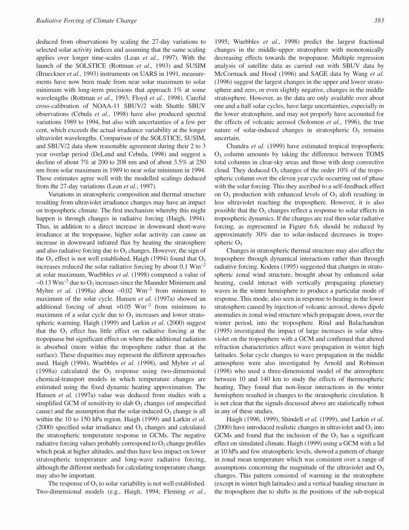
deduced from observations by scaling the 27-day variations toselected solar activity indices and assuming that the same scalingapplies over longer time-scales (Lean et al., 1997). With thelaunch of the SOLSTICE (Rottman et al., 1993) and SUSIM(Brueckner et al., 1993) instruments on UARS in 1991, measure-ments have now been made from near solar maximum to solarminimum with long-term precisions that approach 1% at somewavelengths (Rottman et al., 1993; Floyd et al., 1998). Carefulcross-calibration of NOAA-11 SBUV/2 with Shuttle SBUVobservations (Cebula et al., 1998) have also produced spectralvariations 1989 to 1994, but also with uncertainties of a few percent, which exceeds the actual irradiance variability at the longerultraviolet wavelengths. Comparison of the SOLSTICE, SUSIM,and SBUV/2 data show reasonable agreement during their 2 to 3year overlap period (DeLand and Cebula, 1998) and suggest adecline of about 7% at 200 to 208 nm and of about 3.5% at 250nm from solar maximum in 1989 to near solar minimum in 1994.These estimates agree well with the modelled scalings deducedfrom the 27-day variations (Lean et al., 1997).
Variations in stratospheric composition and thermal structureresulting from ultraviolet irradiance changes may have an impacton tropospheric climate. The first mechanism whereby this mighthappen is through changes in radiative forcing (Haigh, 1994).Thus, in addition to a direct increase in downward short-waveirradiance at the tropopause, higher solar activity can cause anincrease in downward infrared flux by heating the stratosphereand also radiative forcing due to O3 changes. However, the sign ofthe O3 effect is not well established. Haigh (1994) found that O3
increases reduced the solar radiative forcing by about 0.1 Wm−2
at solar maximum, Wuebbles et al. (1998) computed a value of−0.13 Wm−2 due to O3 increases since the Maunder Minimum andMyhre et al. (1998a) about −0.02 Wm−2 from minimum tomaximum of the solar cycle. Hansen et al. (1997a) showed anadditional forcing of about +0.05 Wm−2 from minimum tomaximum of a solar cycle due to O3 increases and lower strato-spheric warming. Haigh (1999) and Larkin et al. (2000) suggestthat the O3 effect has little effect on radiative forcing at thetropopause but significant effect on where the additional radiationis absorbed (more within the troposphere rather than at thesurface). These disparities may represent the different approachesused. Haigh (1994), Wuebbles et al. (1998), and Myhre et al.(1998a) calculated the O3 response using two-dimensionalchemical-transport models in which temperature changes areestimated using the fixed dynamic heating approximation. TheHansen et al. (1997a) value was deduced from studies with asimplified GCM of sensitivity to slab O3 changes (of unspecifiedcause) and the assumption that the solar-induced O3 change is allwithin the 10 to 150 hPa region. Haigh (1999) and Larkin et al.(2000) specified solar irradiance and O3 changes and calculatedthe stratospheric temperature response in GCMs. The negativeradiative forcing values probably correspond to O3 change profileswhich peak at higher altitudes, and thus have less impact on lowerstratospheric temperature and long-wave radiative forcing,although the different methods for calculating temperature changemay also be important.
The response of O3 to solar variability is not well established.Two-dimensional models (e.g., Haigh, 1994; Fleming et al.,
1995; Wuebbles et al., 1998) predict the largest fractionalchanges in the middle-upper stratosphere with monotonicallydecreasing effects towards the tropopause. Multiple regressionanalysis of satellite data as carried out with SBUV data byMcCormack and Hood (1996) and SAGE data by Wang et al.(1996) suggest the largest changes in the upper and lower strato-sphere and zero, or even slightly negative, changes in the middlestratosphere. However, as the data are only available over aboutone and a half solar cycles, have large uncertainties, especially inthe lower stratosphere, and may not properly have accounted forthe effects of volcanic aerosol (Solomon et al., 1996), the truenature of solar-induced changes in stratospheric O3 remainsuncertain.
Chandra et al. (1999) have estimated tropical troposphericO3 column amounts by taking the difference between TOMStotal columns in clear-sky areas and those with deep convectivecloud. They deduced O3 changes of the order 10% of the tropo-spheric column over the eleven year cycle occurring out of phasewith the solar forcing. This they ascribed to a self-feedback effecton O3 production with enhanced levels of O3 aloft resulting inless ultraviolet reaching the troposphere. However, it is alsopossible that the O3 changes reflect a response to solar effects intropospheric dynamics. If the changes are real then solar radiativeforcing, as represented in Figure 6.6, should be reduced byapproximately 30% due to solar-induced decreases in tropo-spheric O3
Changes in stratospheric thermal structure may also affect thetroposphere through dynamical interactions rather than throughradiative forcing. Kodera (1995) suggested that changes in strato-spheric zonal wind structure, brought about by enhanced solarheating, could interact with vertically propagating planetarywaves in the winter hemisphere to produce a particular mode ofresponse. This mode, also seen in response to heating in the lowerstratosphere caused by injection of volcanic aerosol, shows dipoleanomalies in zonal wind structure which propagate down, over thewinter period, into the troposphere. Rind and Balachandran(1995) investigated the impact of large increases in solar ultra-violet on the troposphere with a GCM and confirmed that alteredrefraction characteristics affect wave propagation in winter highlatitudes. Solar cycle changes to wave propagation in the middleatmosphere were also investigated by Arnold and Robinson(1998) who used a three-dimensional model of the atmospherebetween 10 and 140 km to study the effects of thermosphericheating. They found that non-linear interactions in the winterhemisphere resulted in changes to the stratospheric circulation. Itis not clear that the signals discussed above are statistically robustin any of these studies.
Haigh (1996, 1999), Shindell et al. (1999), and Larkin et al.(2000) have introduced realistic changes in ultraviolet and O3 intoGCMs and found that the inclusion of the O3 has a significanteffect on simulated climate. Haigh (1999) using a GCM with a lidat 10 hPa and few stratospheric levels, showed a pattern of changein zonal mean temperature which was consistent over a range ofassumptions concerning the magnitude of the ultraviolet and O3
changes. This pattern consisted of warming in the stratosphere(except in winter high latitudes) and a vertical banding structure inthe troposphere due to shifts in the positions of the sub-tropical
383Radiative Forcing of Climate Change

jets. The predicted changes in 30 hPa geopotential heights were ofsimilar form to those observed by Labitzke and van Loon (1997)but of smaller magnitude (by about a factor 3). Larkin et al. (2000)found very similar patterns of change to those of Haigh (1999)using the same solar irradiance/O3 changes but an entirelydifferent GCM with a lid at 0.1 hPa. Shindell et al. (1999) used amodel with a detailed representation of the middle atmosphereand a parametrized photochemical scheme which allows O3 torespond to changes in ultraviolet flux but not to changes in windfields. They showed larger amplitude changes in 30 hPa heights inthe winter hemisphere, more like those of Labitzke and van Loon(1997) but with little summer hemisphere response. These experi-ments suggest that further work is needed to establish the responseof O3 to solar variability and to how this affects climate.
6.11.2.2 Cosmic rays and cloudsSvensmark and Friis-Christensen (1997) demonstrated a highdegree of correlation between total cloud cover, from the ISCCPC2 data set, and cosmic ray flux between 1984 and 1991. Changesin the heliosphere arising from fluctuations in the Sun’s magneticfield mean that galactic cosmic rays (GCRs) are less able to reachthe Earth when the Sun is more active so the cosmic ray flux isinversely related to solar activity. Svensmark and Friis-Christensen analysed monthly mean data of total cloud using onlydata over the oceans between 60°S and 60°N from geostationarysatellites. They found an increase in cloudiness of 3 to 4% fromsolar maximum to minimum and speculated that (a) increasedGCR flux causes an increase in total cloud and that (b) theincrease in total cloud causes a cooling of climate. Svensmark andFriis-Christensen (1997) also extended this analysis to cover theyears 1980 to 1996 using cloud data from the DMSP and Nimbus-7 satellites and showed that the high correlation with GCR flux ismaintained. However, it was not possible to intercalibrate thedifferent data sets so the validity of the extended data set as ameasure of variations in absolute total cloudiness is open toquestion.
Svensmark (1998) showed that, at least for the limited periodof this study, total cloud varies more closely with GCRs than withthe 10.7 cm solar activity index over the past solar cycle. Onlonger time-scales he also demonstrated that NorthernHemisphere surface temperatures between 1937 and 1994 followvariations in cosmic ray flux and solar cycle length more closelythan total irradiance or sunspot number. There has been a long-term decrease in cosmic ray flux since the late 17th century, asevidenced by the 10Be and 14C cosmogenic isotope records(Stuiver and Reimer, 1993; Beer et al., 1994), and this mirrors thelong-term increase in TSI. However, the TSI reconstruction ofHoyt and Schatten (1993), which is based on solar cycle lengths,does not appear to track the cosmogenic isotope records any moreclosely than that of Lean et al. (1995), which is based on sunspotcycle amplitude (Lean and Rind, 1998). Such use of different solarindices may help to identify which physical mechanisms, if any,are responsible for the apparent meteorological responses to solaractivity.
Kuang et al. (1998) have repeated Svensmark and Friis-Christensen’s analysis of ISCCP data and showed high correla-tions with an El Niño-Southern Osciallation (ENSO) index
difficult to distinguish from the GCR flux. Farrar (2000) showedthat the pattern of change in cloudiness over that period, particu-larly in the Pacific Ocean, corresponds to what would be expectedfor the atmospheric circulation changes characteristic of El Niño.Kernthaler et al. (1999) have also studied the ISCCP dataset, usingboth geostationary and polar orbiter data and suggested that thecorrelation with cosmic ray flux is reduced if high latitude data areincluded. This would not be expected if cosmic rays were directlyinducing increases in cloudiness, as cosmic ray flux is greatest athigh latitudes. Kernthaler et al. (1999), Jørgensen and Hansen(2000), and Gierens and Ponater (1999), also noted that amechanism whereby cosmic rays resulted in greater cloud coverwould be most likely to affect high cloud as ionisation is greatestat these altitudes. Even if high cloud did respond to cosmic rays,it is not clear that this would cause global cooling as for thin highcloud the long-wave warming effects dominate the short-wavecooling effect. Kristjánsson and Kristiansen (2000) have addition-ally analysed the ISCCP D2 dataset, 1989 to 1993, and found littlestatistical evidence of a relationship between GCRs and cloudcover with the possible exception of low marine clouds in mid-latitudes. They also noted that there was no correlation betweenoutgoing long-wave radiation, as represented in ERBE data, andGCRs. Thus the evidence for a cosmic ray impact on cloudinessremains unproven.
A further consideration must be potential physicalmechanisms whereby cosmic rays might enhance cloudiness.Cosmic rays are the principal source of ionisation in the freetroposphere. Furthermore, ionisation rates and atmosphericconductivity are observed to vary with solar activity. Svensmarkand Friis-Christensen (1997) propose that the correlation betweencosmic rays and cloud cover that they observed is due to anincrease in efficiency of charged particles, over uncharged ones, inacting as cloud condensation nuclei. There is evidence for thisoccurring in thunderstorms (Pruppacher and Klett, 1997) but it isnot clear to what extent this affects cloud development. There isalso evidence that ions are sometimes critical in gas-to-particleconversion but again there is no evidence that this has any impacton cloud formation.
In a series of papers, Brian Tinsley has developed a moredetailed mechanism for a link between cosmic rays and cloudiness(e.g., Tinsley, 1996). This is based on the premise that aerosolsionised by cosmic rays are more effective as ice nuclei and causefreezing of supercooled water in clouds. In clouds that are likelyto cause precipitation the latent heat thus released then causesenhanced convection which promotes cyclonic development andhence increased storminess. There is some laboratory evidence tosuggest that charging increases ice nucleation efficiency(Pruppacher, 1973) although there is no observational evidence ofthis process taking place in the atmosphere. Furthermore, only asmall proportion of aerosol particles are capable of acting as icenuclei, depending on chemical composition or shape. There arealso laboratory studies (Abbas and Latham, 1969) which indicatethe existence of “electrofreezing”, but again no evidence in thereal atmosphere. Thus Tinsley’s mechanism is plausible butrequires further observational and modelling studies to establishwhether or not it could be of sufficient magnitude to result in theclaimed effects (Harrison and Shine, 1999).
384 Radiative Forcing of Climate Change
We conclude that mechanisms for the amplification of solarforcing are not well established. Variations in ultraviolet andsolar-induced changes in O3 may have a small effect on radiativeforcing but additionally may affect climate through changing thedistribution of solar heating and thus indirectly through adynamical response. At present there is insufficient evidence toconfirm that cloud cover responds to solar variability.
6.12 Global Warming Potentials
6.12.1 Introduction
Just as radiative forcing provides a simplified means ofcomparing the various factors that are believed to influence theclimate system to one another, Global Warming Potentials(GWPs) are one type of simplified index based upon radiativeproperties that can be used to estimate the potential futureimpacts of emissions of different gases upon the climatesystem in a relative sense. The formulation of GWPs, reasonsfor the choice of various time horizons, and the effects ofclouds, scenarios, and many other factors upon GWP valueswere discussed in detail in IPCC (1994). That discussion willnot be repeated here. Section 6.2 discusses the relationshipbetween radiative forcing and climate response and describesrecent studies that have supported the view that many differentkinds of forcing agents (e.g., various greenhouse gases,sulphate aerosols, solar activity, etc.) yield similar globallyaveraged climate responses per Wm−2 of forcing (albeit withdifferent spatial patterns in some important cases). Theseparallels in global mean climate responses have motivated theuse of simplified measures to estimate in an approximatefashion the relative effects of emissions of different gases onclimate. The emphasis on relative rather than absolute effects(such as computed temperature change) avoids dependenceupon any particular model of climate response.
The impact of greenhouse gas emissions upon theatmosphere is related not only to radiative properties, but alsoto the time-scale characterising the removal of the substancefrom the atmosphere. Radiative properties control the absorp-tion of radiation per kilogram of gas present at any instant, butthe lifetime (or adjustment time, see Chapter 4) controls howlong an emitted kilogram is retained in the atmosphere andhence is able to influence the thermal budget. The climatesystem responds to changes in the thermal budget on time-scales ranging from the order of months to millenniadepending upon processes within the atmosphere, ocean,cryosphere, etc.
GWPs are a measure of the relative radiative effect of agiven substance compared to another, integrated over a chosentime horizon. The choice of the time horizon depends in partupon whether the user wishes to emphasise shorter-termprocesses (e.g., responses of cloud cover to surface tempera-ture changes) or longer-term phenomena (such as sea levelrise) that are linked to sustained alterations of the thermalbudget (e.g., the slow transfer of heat between, for example,the atmosphere and ocean). In addition, if the speed ofpotential climate change is of greatest interest (rather than the
eventual magnitude), then a focus on shorter time horizons canbe useful (IPCC, l994; Skodvin and Fuglestvedt, 1997;Fuglestvedt et al., 2000; Smith and Wigley, 2000a,b).
As in previous reports, here we present GWPs for 20, 100,and 500 year time horizons. The most recent GWP evaluationsare those of WMO (l999) and the SAR, and the results presentedhere are drawn in large part from those assessments, with updatesfor those cases where significantly different new laboratory orradiative transfer results have been published. The sources usedfor input variables for the GWP calculations are indicated in thissection and in the headers and footnotes to the tables, wheresources of new estimates since the SAR are identified.
The GWP has been defined as the ratio of the time-integratedradiative forcing from the instantaneous release of 1 kg of a tracesubstance relative to that of 1 kg of a reference gas (IPCC, l990):
where TH is the time horizon over which the calculation isconsidered, ax is the radiative efficiency due to a unit increasein atmospheric abundance of the substance in question (i.e.,Wm−2 kg−1), [x(t)] is the time-dependent decay in abundance ofthe instantaneous release of the substance, and the correspondingquantities for the reference gas are in the denominator. The GWPof any substance therefore expresses the integrated forcing of apulse (of given small mass) of that substance relative to theintegrated forcing of a pulse (of the same mass) of the referencegas over some time horizon. The numerator of Equation 6.2 is theabsolute (rather than relative) GWP of a given substance, referredto as the AGWP. The GWPs of various greenhouse gases can thenbe easily compared to determine which will cause the greatestintegrated radiative forcing over the time horizon of interest. Thedirect relative radiative forcings per ppbv are derived frominfrared radiative transfer models based on laboratory measure-ments of the molecular properties of each substance and consid-ering the molecular weights. Updated information since the SARis presented for many gases in Section 6.3. Many importantchanges in these quantities were recently reviewed in WMO(l999) and will be briefly summarised here. In addition, somegases can indirectly affect radiative forcing, mainly throughchemical processes. For example, tropospheric O3 provides asignificant radiative forcing of the climate system, but its produc-tion occurs indirectly, as a result of atmospheric chemistryfollowing emissions of precursors such as NOx, CO, andNMHCs (see Section 6.6 and Chapter 4). Indirect effects will bedescribed below for a number of key gases.
It is important to distinguish between the integrated relativeeffect of an emitted kilogram of gas which is represented by aGWP and the actual radiative forcings for specific gas amountspresented, for example, in Section 6.3 and in Figure 6.6. GWPsare intended for use in studying relative rather than absoluteimpacts of emissions, and pertain to specific time horizons.
The radiative efficiencies ar and ax are not necessarilyconstant over time. While the absorption of infrared radiation bymany greenhouse gases varies linearly with their abundance, a
385Radiative Forcing of Climate Change
TH
∫ ax • [x(t)] dt0
TH
∫ ar • [r(t)] dt0
GWP(x) = (6.2)
few important ones display non-linear behaviour for current andlikely future abundances (e.g., CO2, CH4, and N2O). For thosegases, the relative radiative forcing will depend upon abundanceand hence upon the future scenario adopted. These issues werediscussed in detail and some sensitivities to chosen scenarioswere presented in IPCC (l994).
A key aspect of GWP calculations is the choice of thereference gas, taken here to be CO2. In IPCC (l994), it wasshown, for example, that a particular scenario for future growthof CO2 (S650, see Chapter 3) would change the denominator ofEquation 6.2 by as much as 15% compared to a calculationemploying constant pre-industrial CO2 mixing ratios.
The atmospheric response time of CO2 is subject tosubstantial scientific uncertainties, due to limitations in ourknowledge of key processes including its uptake by thebiosphere and ocean. When CO2 is used as the reference, thenumerical values of the GWPs of all greenhouse gases canchange substantially as research improves the understanding ofthe removal processes of CO2. The removal function for CO2
used for the GWPs presented here is based upon carbon cyclemodels such as those discussed in Chapter 3. The CO2 radiativeefficiency (ar) used in this report has been updated since theSAR, as discussed in Section 6.3 (see below).
The lifetimes of non-CO2 greenhouse gases are dependentlargely on atmospheric photochemistry, which controls photo-lysis and related removal processes as discussed in Chapter 4.When the lifetime of the gas in question is comparable to theresponse time of CO2 (nominally about 150 years, although it isclear that the removal of CO2 cannot be adequately describedby a single, simple exponential lifetime; see IPCC (l994) andthe discussion below), the GWP is relatively insensitive tochoice of time horizon, i.e., for N2O. When the lifetime of thegas in question differs substantially from the response time ofthe reference gas, the GWP becomes sensitive to the choice oftime horizon, which in turn implies a decision regarding theclimate processes and impacts of interest, as noted above. Forlonger time horizons, those species that decay more rapidlythan the reference gas display decreasing GWPs, with the slopeof the decay being dependent mainly on the lifetime of the gasin question. Gases with lifetimes much longer than that of thereference gas (e.g., C2F6) display increasing GWPs over longtime horizons (i.e., greater than a hundred years). We emphasisethat the GWP is an integral from zero to the chosen timehorizon; hence the values presented in the table for 25, 100, and500 years are not additive.
A number of studies have suggested modified or differentindices for evaluating relative future climate effects. Here weprovide only an indication of the kinds of issues that are beingconsidered in these alternative indices. Wuebbles and Calm(l997) emphasised the fact that some halocarbon substitutesused, for example, in refrigeration are less efficient than theCFCs they are replacing, so that more energy is consumedthrough their use and hence more CO2 emitted per hour ofoperation. Evaluation of these technological factors would onlybe possible through detailed emission inventories coupled withscenarios, and are not included here. Some studies have arguedfor use of “discount rates” to reflect increasing uncertainty and
changing policies with time (e.g., to account for the possibilitythat new technologies will emerge to solve problems; see forexample Lashof and Ahuja, l990; Reilly et al., l999). Economicfactors could be considered along with the technological onesmentioned above, adding another aspect to any scenario. Theseare not included here. Smith and Wigley (2000a,b), Fuglestvedtet al. (2000), and Reilly et al. (l999) have examined therelationship between GWPs and climate response using simpleenergy balance models. These studies emphasised the pointmade above regarding the links between choice of time horizon,lifetime of a particular substance, and the climate response ofinterest, noting for example that while the 100-year GWP forN2O represented the model-calculated temperature responses(both instantaneous and integrated over time), and thecalculated sea level rise to good accuracy, that for CH4 (a short-lived gas with a lifetime of about 10 years) represented sea levelrise far better than it did the instantaneous temperature changefor that time horizon. For very short-lived gases, GWPs areoften calculated using a ‘slab’ (continuous) rather than pulseemission. This approach involves the assumption of specificscenarios for the magnitudes of the slabs. For some very short-lived gases such as NMHCs, models must employ ‘slab’emissions in GWP analyses since their impact dependscritically on non-linear coupled chemical processes. Someexamples are given in Sections 6.12.3.2 and 6.12.3.4.
6.12.2 Direct GWPs
The CO2 response function used in this report is the same as thatin WMO (l999) and the SAR and is based on the “Bern” carboncycle model (see Siegenthaler and Joos, 1992; Joos et al., l996)run for a constant future mixing ratio of CO2 over a period of500 years. The Bern carbon cycle model was compared to othersin IPCC (l994), where it was shown that different models gave arange of as much as 20% in the CO2 response, with the greatestdifferences occurring over time-scales greater than 20 years.
The radiative efficiency per kilogram of CO2 has beenupdated compared to previous IPCC assessments (IPCC, 1994;SAR). Here we employ the approach discussed in WMO (l999)using the simplified formula presented in Table 6.2. We assumea background CO2 mixing ratio of 364 ppmv, close to the presentday value (WMO (1995) used 354 ppmv). For this assumption,this expression agrees well with the adjusted total-sky radiativeforcing calculations of Myhre and Stordal (1997); see alsoMyhre et al. (1998b). The revised forcing is about 12% lowerthan that in the SAR. For a small perturbation in CO2 from 364ppmv, the radiative efficiency is 0.01548 Wm−2 ppmv−1. Thisvalue is used in the GWP calculations presented here. Weemphasise that it applies only to GWP calculations and cannotbe used to obtain the total radiative forcing for this key gas sincepre-industrial times, due to time-dependent changes in mixingratio as noted above. Because of this change in the CO2 forcingper mass, the CO2 AGWPs are 0.207, 0.696, and 2.241 Wm−2/yr/ppmv−1 for 20, 100, and 500 year time horizons, respectively.These are smaller than the values used in the SAR by 13%.AGWPs for any gas can be obtained from the GWP values givenin the tables presented here by multiplying by these numbers.
386 Radiative Forcing of Climate Change

The decreases in the CO2 AGWPs will lead to proportion-ately larger GWPs for other gases compared to previous IPCCassessments, in the absence of other changes. In Tables 6.7 and6.8, GWPs (on a mass basis) for 93 gases are tabulated for timehorizons of 20, 100, and 500 years. The list includes CH4, N2O,CFCs, HCFCs, HFCs, hydrochlorocarbons, bromocarbons,iodocarbons, fully fluorinated species, fluoroalcohols, andfluoroethers. The radiative efficiencies per kilogram were derivedfrom the values given per ppbv in Section 6.3. Several of thesehave been updated since the SAR, most notably that of CFC-11.Since the radiative forcings of the halocarbon replacement gasesare scaled relative to CFC-11 in GWP calculations, the GWPs ofthose gases are also affected by this change. As discussed furtherin Section 6.3, the change in radiative forcing for CFC-11 reflectsnew studies (Pinnock et al., 1995; Christidis et al., l997; Hansenet al., l997a; Myhre and Stordal, 1997; Good et al., 1998)suggesting that the radiative forcing of this gas is about 0.25Wm−2 ppbv−1, an increase of about 14% compared to the valueadopted in earlier IPCC reports, which was based on the study ofHansen et al. (l988).
The lifetimes and adjustment times used in Tables 6.7 and6.8 come from Chapter 4 except where noted. For some gases(including several of the fluoroethers), lifetimes have not beenderived from laboratory measurements, but have been estimatedby various other means. For this reason, the lifetimes for thesegases, and hence the GWPs, are considered to be much lessreliable, and so these gases are listed separately in Table 6.8. NF3
is listed in Table 6.8 because, although its photolytic destructionhas been characterised, other loss processes may be significantbut have not yet been characterised (Molina et al., 1995). Notealso that some gases, for example, trifluoromethyl iodide (CF3I)and dimethyl ether (CH3OCH3) have very short lifetimes (lessthan a few months); GWPs for such very short-lived gases mayneed to be treated with caution, because the gases are unlikely tobe evenly distributed globally, and hence estimates of, forexample, their radiative forcing using global mean conditionsmay be subject to error.
Uncertainties in the lifetimes of CFC-11 and CH3CCl3 arethought to be about 10%, while uncertainties in the lifetimes ofgases obtained relative to CFC-11 or CH3CCl3 are somewhatlarger (20 to 30%) (SAR; WMO, l999). Uncertainties in theradiative forcing per unit mass of the majority of the gasesconsidered in Table 6.7 are approximately ± 10%. The SARsuggested typical uncertainties of ± 35% (relative to the referencegas) for the GWPs, and we retain this uncertainty estimate forgases listed in Table 6.7. In addition to uncertainties in the CO2
radiative efficiency per kilogram and in the response function,AGWPs of CO2 are affected by assumptions concerning futureCO2 abundances as noted above. Furthermore, as the CO2 mixingratios and climate change, the pulse response function changes aswell. In spite of these dependencies on the choice of futureemission scenarios, it remains likely that the error introduced bythese assumptions is smaller than the uncertainties introduced byour imperfect understanding of the carbon cycle (see Chapter 3).Finally, although any induced error in the CO2 AGWPs willcertainly affect the non-CO2 GWPs, it will not affect intercom-parisons among non-CO2 GWPs.
6.12.3 Indirect GWPs
We next consider discuss indirect effects in more detail, andpresent GWPs for other gases, including estimates of theirimpacts. While direct GWPs are usually believed to be knownreasonably accurately (±35%), indirect GWPs can be highlyuncertain. A number of different processes contribute to indirecteffects for various molecules; many of these are also discussed inSection 6.6.
6.12.3.1 MethaneFour types of indirect effects due to the presence of atmosphericCH4 have been identified (see Chapter 4 and Section 6.6). Thelargest effect is potentially the production of O3 (25% of thedirect effect, or 19% of the total, as in the SAR). This effect isdifficult to quantify, however, because the magnitude of O3
production is highly dependent on the abundance and distributionof NOx (IPCC, 1994; SAR). Other indirect effects include theproduction of stratospheric water vapour (assumed here torepresent 5% of the direct effect, or 4% of the total, as in theSAR), the production of CO2 (from certain CH4 sources), and thetemporal changes in the CH4 adjustment time resulting from itscoupling with OH (Lelieveld and Crutzen, 1992; Brühl, 1993;Prather, 1994, 1996; SAR; Fuglestvedt et al., 1996). Here weadopt the values for each of these terms as given in the SAR, witha correction for the updated CO2 AGWPs and adopting theperturbation lifetime given in Chapter 4. It should be noted thatthe climate forcing caused by CO2 produced from the oxidationof CH4 is not included in these GWP estimates. As discussed inthe SAR, it is often the case that this CO2 is included in nationalcarbon production inventories. Therefore, depending on how theinventories are combined, including the CO2 production fromCH4 could result in double counting this CO2.
6.12.3.2 Carbon monoxideCO has a small direct GWP but leads to indirect radiative effectsthat are similar to those of CH4. As in the case of CH4, theproduction of CO2 from oxidised CO can lead to double countingof this CO2 and is therefore not considered here. The emission ofCO perturbs OH, which in turn can then lead to an increase in theCH4 lifetime (Fuglestvedt et al., l996; Prather, 1996; Daniel andSolomon, 1998). This term involves the same processes wherebyCH4 itself influences its own lifetime and hence GWP values(Prather, l996) and is subject to similar uncertainty. This term canbe evaluated with reasonable accuracy using a box model, asshown by Prather (l996) and Daniel and Solomon (1998).Emissions of CO can also lead to the production of O3 (seeChapter 4), with the magnitude of O3 formation dependent on theamount of NOx present. As with CH4, this effect is quite difficultto quantify due to the highly variable and uncertain NOx distri-bution (e.g., Emmons et al., 1997). Because of the difficulty inaccurately calculating the amount of O3 produced by COemissions, an accurate estimate of the entire indirect forcing ofCO requires a three-dimensional chemical model. Table 6.9presents estimates of the CO GWP due to O3 production and tofeedbacks on the CH4 cycle from two recent multi-dimensionalmodel studies (in which a “slab” emission of CO was imposed),
387Radiative Forcing of Climate Change

388 Radiative Forcing of Climate Change
Gas Radiativeefficiency
(Wm−2 ppb−1)
Lifetime (years)(from Chapter 4
Global Warming Potential
Time horizon(from (b)
unless indicated)
unless indicated)20
years100
years500
years
Carbon dioxide CO2 See Section 6.12.2 See Section 6.12.2 1 1 1Methane CH4 3.7x10⁻⁴ ∑ 12.0* 62 23 7Nitrous oxide N2O 3.1x10⁻³ ∑ 114* 275 296 156
ChlorofluorocarbonsCFC-11 CCl3F 0.25 45 6300 4600 1600CFC-12 CCl2F2 0.32 100 10200 10600 5200CFC-13 CClF3 0.25 640 (c) 10000 14000 16300CFC-113 CCl2FCClF2 0.30 85 6100 6000 2700CFC-114 CClF2CClF2 0.31 300 7500 9800 8700CFC-115 CF3CClF2 0.18† 1700 4900 7200 9900
HydrochlorofluorocarbonsHCFC-21 CHCl2F 0.17 2.0 (d) 700 210 65HCFC-22 CHClF2 0.20§ 11.9 4800 1700 540HCFC-123 CF3 CHCl2 0.20 1.4 (a) 390 120 36HCFC-124 CF3CHClF 0.22 6.1 (a) 2000 620 190HCFC-141b CH3CCl2F 0.14 9.3 2100 700 220HCFC-142b CH3CClF2 0.20 19 5200 2400 740HCFC-225ca CF3CF2CHCl2 0.27 2.1 (a) 590 180 55HCFC-225cb CClF2CF2CHClF 0.32 6.2 (a) 2000 620 190
HydrofluorocarbonsHFC-23 CHF3 0.16§ 260 9400 12000 10000HFC-32 CH2F2 0.09§ 5.0 1800 550 170HFC-41 CH3F 0.02 2.6 330 97 30HFC-125 CHF2CF3 0.23§ 29 5900 3400 1100HFC-134 CHF2CHF2 0.18 9.6 3200 1100 330HFC-134a CH2FCF3 0.15§ 13.8 3300 1300 400HFC-143 CHF2CH2F 0.13 3.4 1100 330 100HFC-143a CF3CH3 0.13§ 52 5500 4300 1600HFC-152 CH2FCH2 F 0.09 0.5 140 43 13HFC-152a CH3CHF2 0.09§ 1.4 410 120 37HFC-161 CH3CH2F 0.03 0.3 40 12 4HFC-227ea CF3CHFCF3 0.30 33.0 5600 3500 1100HFC-236cb CH2FCF2CF3 0.23 13.2 3300 1300 390HFC-236ea CHF2CHFCF3 0.30 10.0 3600 1200 390HFC-236fa CF3CH2CF3 0.28 220 7500 9400 7100HFC-245ca CH2FCF2CHF2 0.23 5.9 2100 640 200HFC-245fa CHF2CH2CF3 0.28& 7.2 3000 950 300HFC-365mfc CF3CH2CF2CH3 0.21 (k) 9.9 2600 890 280HFC-43-10mee CF3CHFCHFCF2CF3 0.40 15 3700 1500 470
ChlorocarbonsCH3CCl3 0.06 4.8 450 140 42CCl4 0.13†† 35 2700 1800 580CHCl3 0.11§ 0.51 (a) 100 30 9CH3Cl 0.01 1.3 (b) 55 16 5CH2Cl2 0.03 0.46 (a) 35 10 3
Table 6.7: Direct Global Warming Potentials (mass basis) relative to carbon dioxide (for gases for which the lifetimes have been adequatelycharacterised).
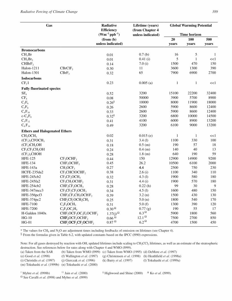
389Radiative Forcing of Climate Change
* The values for CH4 and N2O are adjustment times including feedbacks of emission on lifetimes (see Chapter 4).∑ From the formulas given in Table 6.2, with updated constants based on the IPCC (l990) expressions.
Note: For all gases destroyed by reaction with OH, updated lifetimes include scaling to CH3CCl3 lifetimes, as well as an estimate of the stratosphericdestruction. See references below for rates along with Chapter 4 and WMO (l999).(a) Taken from the SAR (b) Taken from WMO (l999) (c) Taken from WMO (1995) (d) DeMore et al. (1997)(e) Good et al. (1998) (f) Wallington et al. (1997) (g) Christensen et al. (1998) (h) Heathfield et al. (1998a)(i) Christidis et al. (1997) (j) Gierczak et al. (1996) (k) Barry et al. (1997) (l) Tokuhashi et al. (1999a)(m) Tokuhashi et al. (1999b) (n) Tokuhashi et al. (2000)
† Myhre et al. (l998b) †† Jain et al. (2000) § Highwood and Shine (2000) & Ko et al. (l999).Ω See Cavalli et al. (l998) and Myhre et al. (l999)
Gas RadiativeEfficiency
(Wm−2 ppb−1)
Lifetime (years)(from Chapter 4
Global Warming Potential
Time horizon(from (b)
unless indicated)
unless indicated)20
years100
years500
years
BromocarbonsCH3Br 0.01 0.7 (b) 16 5 1CH2Br2 0.01 0.41 (i) 5 1 <<1CHBrF2 0.14 7.0 (i) 1500 470 150Halon-1211 CBrClF2 0.30 11 3600 1300 390Halon-1301 CBrF3 0.32 65 7900 6900 2700
IodocarbonsCF3 I 0.23 0.005 (a) 1 1 <<1
Fully fluorinated speciesSF6 0.52 3200 15100 22200 32400CF4 0.08 50000 3900 5700 8900C2F6 0.26§ 10000 8000 11900 18000C3F8 0.26 2600 5900 8600 12400C4F10 0.33 2600 5900 8600 12400c-C4F8 0.32§ 3200 6800 10000 14500C5F12 0.41 4100 6000 8900 13200C6 F14 0.49 3200 6100 9000 13200
Ethers and Halogenated EthersCH3OCH3 0.02 0.015 (e) 1 1 <<1(CF3)2CFOCH3 0.31 3.4 (l) 1100 330 100(CF3)CH2OH 0.18 0.5 (m) 190 57 18CF3CF2CH2OH 0.24 0.4 (m) 140 40 13(CF3)2CHOH 0.28 1.8 (m) 640 190 59HFE-125 CF3OCHF2 0.44 150 12900 14900 9200HFE-134 CHF2OCHF2 0.45 26.2
4.410500 6100 2000
HFE-143a CH3OCF3 0.27 4.4 2500 750 230HCFE-235da2 CF3CHClOCHF2 0.38 2.6 (i) 1100 340 110HFE-245cb2 CF3CF2OCH3 0.32 4.3 (l) 1900 580 180HFE-245fa2 CF3CH2OCHF2 0.31 4.4 (i) 1900 570 180HFE-254cb2 CHF2CF2OCH3 0.28 0.22 (h) 99 30 9HFE-347mcc3 CF3CF2CF2OCH3 0.34 4.5 (l) 1600 480 150HFE-356pcf3 CHF2CF2CH2OCHF2 0.39 3.2 (n) 1500 430 130HFE-374pc2 CHF CF22 OCH2CH3 0.25 5.0 (n) 1800 540 170HFE-7100 C4F9OCH3 0.31 5.0 (f) 1300 390 120HFE-7200 C4F9OC2H5 0.30 0.77 (g) 190 55 17H-Galden 1040x CHF2OCF2OC2F4O
CHF2
1.37(j) 6.3 5900 1800 560HG-10 CHF2OCF2OCHF2
CHF OCF CF OC0.66 12.1 7500 2700 850
HG-01 CHF2OCF2CF2OCHF2
CHF2
0.87 6.2 4700 1500 450
Ω
Ω
ΩΩ
Ω
Ω
Ω
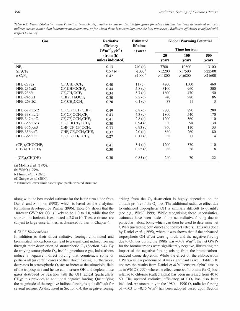
along with the box-model estimate for the latter term alone fromDaniel and Solomon (l998), which is based on the analyticalformalism developed by Prather (l996). Table 6.9 shows that the100-year GWP for CO is likely to be 1.0 to 3.0, while that forshorter time horizons is estimated at 2.8 to 10. These estimates aresubject to large uncertainties, as discussed further in Chapter 4.
6.12.3.3 HalocarbonsIn addition to their direct radiative forcing, chlorinated andbrominated halocarbons can lead to a significant indirect forcingthrough their destruction of stratospheric O3 (Section 6.4). Bydestroying stratospheric O3, itself a greenhouse gas, halocarbonsinduce a negative indirect forcing that counteracts some orperhaps all (in certain cases) of their direct forcing. Furthermore,decreases in stratospheric O3 act to increase the ultraviolet fieldof the troposphere and hence can increase OH and deplete thosegases destroyed by reaction with the OH radical (particularlyCH4); this provides an additional negative forcing. Quantifyingthe magnitude of the negative indirect forcing is quite difficult forseveral reasons. As discussed in Section 6.4, the negative forcing
arising from the O3 destruction is highly dependent on thealtitude profile of the O3 loss. The additional radiative effect dueto enhanced tropospheric OH is similarly difficult to quantify(see e.g., WMO, l999). While recognising these uncertainties,estimates have been made of the net radiative forcing due toparticular halocarbons, which can then be used to determine netGWPs (including both direct and indirect effects). This was doneby Daniel et al. (1995), where it was shown that if the enhancedtropospheric OH effect were ignored, and the negative forcingdue to O3 loss during the 1980s was −0.08 Wm−2, the net GWPsfor the bromocarbons were significantly negative, illustrating theimpact of the negative forcing arising from the bromocarbon-induced ozone depletion. While the effect on the chlorocarbonGWPs was less pronounced, it was significant as well. Table 6.10updates the results from Daniel et al.’s “constant-alpha” case Aas in WMO (l999), where the effectiveness of bromine for O3 lossrelative to chlorine (called alpha) has been increased from 40 to60. The updated radiative efficiency of CO2 has also beenincluded. An uncertainty in the 1980 to 1990 O3 radiative forcingof −0.03 to −0.15 Wm−2 has been adopted based upon Section
390 Radiative Forcing of Climate Change
Gas Radiativeefficiency
(Wm−2 ppb−1)
Estimatedlifetime(years)
Global Warming Potential
Time horizon
(from (b)unless indicated)
20years
100years
500years
NF3 0.13 740 (a) 7700 10800 13100SF5 CF3 0.57 (d) >1000* >12200 >17500 >22500c-C3F6 0.42 >1000* >11800 >16800 >21600
HFE-227ea CF3CHFOCF3 0.40 11 (c) 4200 1500 460HFE-236ea2 CF3CHFOCHF2 0.44 5.8 (c) 3100 960 300HFE-236fa CF3CH2OCF3 0.34 3.7 (c) 1600 470 150HFE-245fa1 CHF2CH2OCF3 0.30 2.2 (c) 940 280 86HFE-263fb2 CF3CH2OCH3 0.20 0.1 (c) 37 11 3
HFE-329mcc2 CF3CF2OCF2CHF2 0.49 6.8 (c) 2800 890 280HFE-338mcf2 CF3CF2OCH2CF3 0.43 4.3 (c) 1800 540 170HFE-347mcf2 CF3CF2OCH2CHF2 0.41 2.8 (c) 1200 360 110HFE-356mec3 CF3CHFCF2 OCH3 0.30 0.94 (c) 330 98 30HFE-356pcc3 CHF2CF2 CF2OCH3 0.33 0.93 (c) 360 110 33HFE-356pcf2 CHF2 CF2OCH2 2CHF 0.37 2.0 (c) 860 260 80HFE-365mcf3 CF3CF2CH2OCH3 0.27 0.11 (c) 38 11 4
(CF3)2CHOCHF2 0.41 3.1 (c) 1200 370 110(CF3)2 CHOCH3 0.30 0.25 (c) 88 26 8
-(CF2)4CH(OH)- 0.30 0.85 (c) 240 70 22
Table 6.8: Direct Global Warming Potentials (mass basis) relative to carbon dioxide (for gases for whose lifetime has been determined only viaindirect means, rather than laboratory measurements, or for whom there is uncertainty over the loss processes). Radiative efficiency is defined withrespect to all sky.
(a) Molina et al. (1995).(b) WMO (1999).(c) Imasu et al. (1995).(d) Sturges et al. (2000).* Estimated lower limit based upon perfluorinated structure.
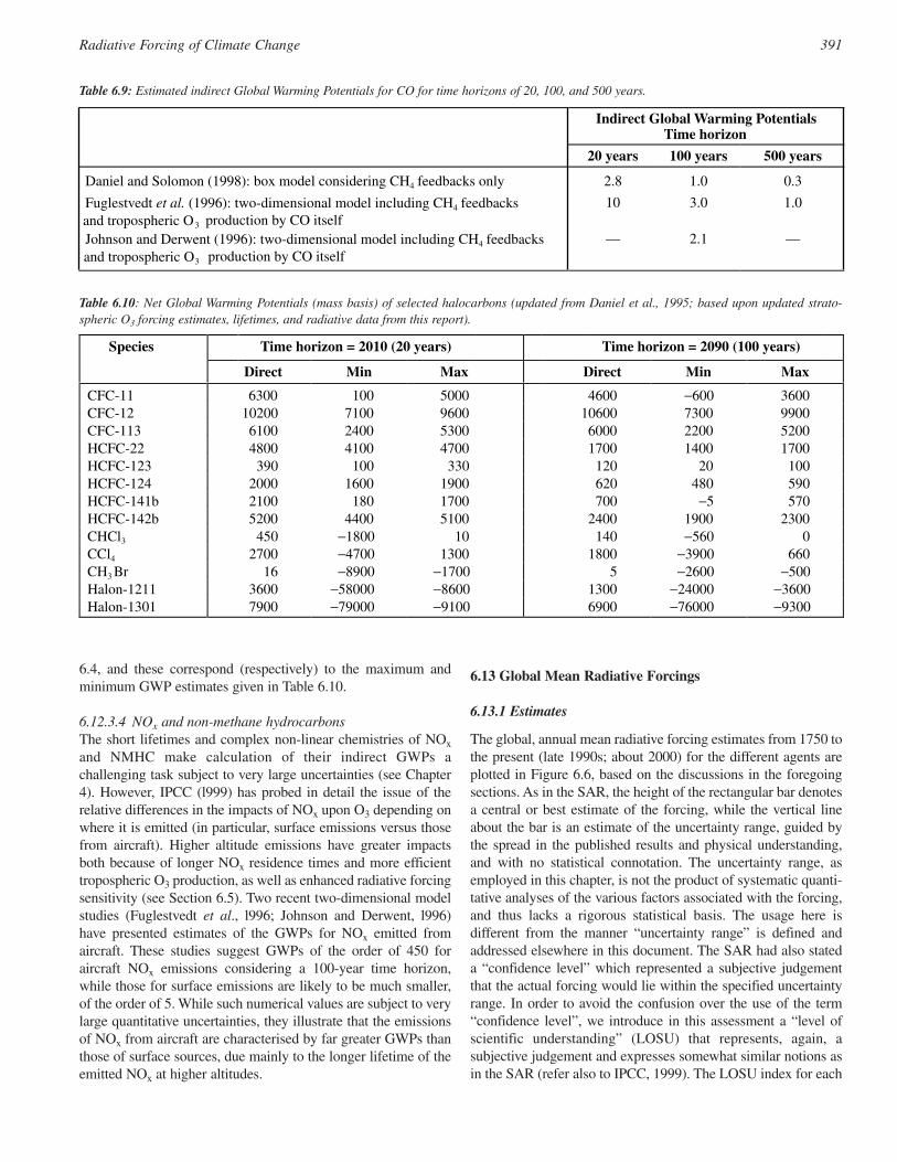
6.4, and these correspond (respectively) to the maximum andminimum GWP estimates given in Table 6.10.
6.12.3.4 NOx and non-methane hydrocarbonsThe short lifetimes and complex non-linear chemistries of NOx
and NMHC make calculation of their indirect GWPs achallenging task subject to very large uncertainties (see Chapter4). However, IPCC (l999) has probed in detail the issue of therelative differences in the impacts of NOx upon O3 depending onwhere it is emitted (in particular, surface emissions versus thosefrom aircraft). Higher altitude emissions have greater impactsboth because of longer NOx residence times and more efficienttropospheric O3 production, as well as enhanced radiative forcingsensitivity (see Section 6.5). Two recent two-dimensional modelstudies (Fuglestvedt et al., l996; Johnson and Derwent, l996)have presented estimates of the GWPs for NOx emitted fromaircraft. These studies suggest GWPs of the order of 450 foraircraft NOx emissions considering a 100-year time horizon,while those for surface emissions are likely to be much smaller,of the order of 5. While such numerical values are subject to verylarge quantitative uncertainties, they illustrate that the emissionsof NOx from aircraft are characterised by far greater GWPs thanthose of surface sources, due mainly to the longer lifetime of theemitted NOx at higher altitudes.
6.13 Global Mean Radiative Forcings
6.13.1 Estimates
The global, annual mean radiative forcing estimates from 1750 tothe present (late 1990s; about 2000) for the different agents areplotted in Figure 6.6, based on the discussions in the foregoingsections. As in the SAR, the height of the rectangular bar denotesa central or best estimate of the forcing, while the vertical lineabout the bar is an estimate of the uncertainty range, guided bythe spread in the published results and physical understanding,and with no statistical connotation. The uncertainty range, asemployed in this chapter, is not the product of systematic quanti-tative analyses of the various factors associated with the forcing,and thus lacks a rigorous statistical basis. The usage here isdifferent from the manner “uncertainty range” is defined andaddressed elsewhere in this document. The SAR had also stateda “confidence level” which represented a subjective judgementthat the actual forcing would lie within the specified uncertaintyrange. In order to avoid the confusion over the use of the term“confidence level”, we introduce in this assessment a “level ofscientific understanding” (LOSU) that represents, again, asubjective judgement and expresses somewhat similar notions asin the SAR (refer also to IPCC, 1999). The LOSU index for each
391Radiative Forcing of Climate Change
Table 6.9: Estimated indirect Global Warming Potentials for CO for time horizons of 20, 100, and 500 years.
Indirect Global Warming PotentialsTime horizon
20 years 100 years 500 years
Daniel and Solomon (1998): box model considering CH4 feedbacks only 2.8 1.0 0.3
Fuglestvedt et al. (1996): two-dimensional model including CH4 feedbacks and tropospheric O3 production by CO itself
10 3.0 1.0
Johnson and Derwent (1996): two-dimensional model including CH4 feedbacks and tropospheric O3 production by CO itself
— 2.1 —
Table 6.10: Net Global Warming Potentials (mass basis) of selected halocarbons (updated from Daniel et al., 1995; based upon updated strato-spheric O3 forcing estimates, lifetimes, and radiative data from this report).
Species Time horizon = 2010 (20 years) Time horizon = 2090 (100 years)
Direct Min Max Direct Min Max
CFC-11 6300 100 5000 4600 −600 3600CFC-12 10200 7100 9600 10600 7300 9900CFC-113 6100 2400 5300 6000 2200 5200HCFC-22 4800 4100 4700 1700 1400 1700HCFC-123 390 100 330 120 20 100HCFC-124 2000 1600 1900 620 480 590HCFC-141b 2100 180 1700 700 −5 570HCFC-142b 5200 4400 5100 2400 1900 2300CHCl3 450 −1800 10 140 −560 0CCl4 2700 −4700 1300 1800 −3900 660CH3 Br 16 −8900 −1700 5 −2600 −500Halon-1211 3600 −58000 −8600 1300 −24000 −3600Halon-1301 7900 −79000 −9100 6900 −76000 −9300
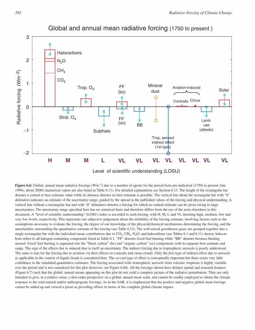
392 Radiative Forcing of Climate Change
Level of scientific understanding (LOSU)
−2
−1
0
1
2
3
Rad
iativ
e fo
rcin
g (
Wm
−2)
Global and annual mean radiative forcing (1750 to present )
H M M L VL VL VL VL VLVL
CO2
VL
CH4
N2O
Halocarbons
Strat. O3
Trop. O3
Sulphate
FF(bc)
FF(oc) BB
dust
Contrails
SolarMineral
Trop. aerosolindirect effect
(1st type)
Land-use
(albedo)
Cirrus
VL
Aviation-induced
Figure 6.6: Global, annual mean radiative forcings (Wm−2) due to a number of agents for the period from pre-industrial (1750) to present (late1990s; about 2000) (numerical values are also listed in Table 6.11). For detailed explanations see Section 6.13. The height of the rectangular bardenotes a central or best estimate value while its absence denotes no best estimate is possible. The vertical line about the rectangular bar with “x”delimiters indicates an estimate of the uncertainty range, guided by the spread in the published values of the forcing and physical understanding. Avertical line without a rectangular bar and with “o” delimiters denotes a forcing for which no central estimate can be given owing to largeuncertainties. The uncertainty range specified here has no statistical basis and therefore differs from the use of the term elsewhere in thisdocument. A “level of scientific understanding” (LOSU) index is accorded to each forcing, with H, M, L and VL denoting high, medium, low andvery low levels, respectively. This represents our subjective judgement about the reliability of the forcing estimate, involving factors such as theassumptions necessary to evaluate the forcing, the degree of our knowledge of the physical/chemical mechanisms determining the forcing, and theuncertainties surrounding the quantitative estimate of the forcing (see Table 6.12). The well-mixed greenhouse gases are grouped together into asingle rectangular bar with the individual mean contributions due to CO2, CH4, N2O, and halocarbons (see Tables 6.1 and 6.11) shown; halocar-bons refers to all halogen-containing compounds listed in Table 6.1. “FF” denotes fossil fuel burning while “BB” denotes biomass burningaerosol. Fossil fuel burning is separated into the “black carbon” (bc) and “organic carbon” (oc) components with its separate best estimate andrange. The sign of the effects due to mineral dust is itself an uncertainty. The indirect forcing due to tropospheric aerosols is poorly understood.The same is true for the forcing due to aviation via their effects on contrails and cirrus clouds. Only the first type of indirect effect due to aerosolsas applicable in the context of liquid clouds is considered here. The second type of effect is conceptually important but there exists very littleconfidence in the simulated quantitative estimates. The forcing associated with stratospheric aerosols from volcanic eruptions is highly variableover the period and is not considered for this plot (however, see Figure 6.8d). All the forcings shown have distinct spatial and seasonal features(Figure 6.7) such that the global, annual means appearing on this plot do not yield a complete picture of the radiative perturbation. They are onlyintended to give, in a relative sense, a first-order perspective on a global, annual mean scale, and cannot be readily employed to obtain the climateresponse to the total natural and/or anthropogenic forcings. As in the SAR, it is emphasised that the positive and negative global mean forcingscannot be added up and viewed a priori as providing offsets in terms of the complete global climate impact.
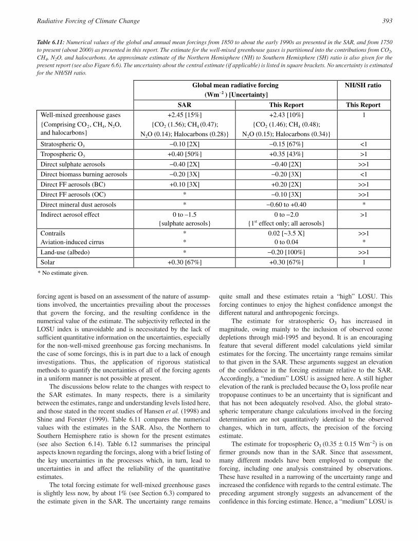
forcing agent is based on an assessment of the nature of assump-tions involved, the uncertainties prevailing about the processesthat govern the forcing, and the resulting confidence in thenumerical value of the estimate. The subjectivity reflected in theLOSU index is unavoidable and is necessitated by the lack ofsufficient quantitative information on the uncertainties, especiallyfor the non-well-mixed greenhouse gas forcing mechanisms. Inthe case of some forcings, this is in part due to a lack of enoughinvestigations. Thus, the application of rigorous statisticalmethods to quantify the uncertainties of all of the forcing agentsin a uniform manner is not possible at present.
The discussions below relate to the changes with respect tothe SAR estimates. In many respects, there is a similaritybetween the estimates, range and understanding levels listed here,and those stated in the recent studies of Hansen et al. (1998) andShine and Forster (1999). Table 6.11 compares the numericalvalues with the estimates in the SAR. Also, the Northern toSouthern Hemisphere ratio is shown for the present estimates(see also Section 6.14). Table 6.12 summarises the principalaspects known regarding the forcings, along with a brief listing ofthe key uncertainties in the processes which, in turn, lead touncertainties in and affect the reliability of the quantitativeestimates.
The total forcing estimate for well-mixed greenhouse gasesis slightly less now, by about 1% (see Section 6.3) compared tothe estimate given in the SAR. The uncertainty range remains
quite small and these estimates retain a “high” LOSU. Thisforcing continues to enjoy the highest confidence amongst thedifferent natural and anthropogenic forcings.
The estimate for stratospheric O3 has increased inmagnitude, owing mainly to the inclusion of observed ozonedepletions through mid-1995 and beyond. It is an encouragingfeature that several different model calculations yield similarestimates for the forcing. The uncertainty range remains similarto that given in the SAR. These arguments suggest an elevationof the confidence in the forcing estimate relative to the SAR.Accordingly, a “medium” LOSU is assigned here. A still higherelevation of the rank is precluded because the O3 loss profile neartropopause continues to be an uncertainty that is significant andthat has not been adequately resolved. Also, the global strato-spheric temperature change calculations involved in the forcingdetermination are not quantitatively identical to the observedchanges, which in turn, affects, the precision of the forcingestimate.
The estimate for tropospheric O3 (0.35 ± 0.15 Wm−2) is onfirmer grounds now than in the SAR. Since that assessment,many different models have been employed to compute theforcing, including one analysis constrained by observations.These have resulted in a narrowing of the uncertainty range andincreased the confidence with regards to the central estimate. Thepreceding argument strongly suggests an advancement of theconfidence in this forcing estimate. Hence, a “medium” LOSU is
393Radiative Forcing of Climate Change
Table 6.11: Numerical values of the global and annual mean forcings from 1850 to about the early 1990s as presented in the SAR, and from 1750to present (about 2000) as presented in this report. The estimate for the well-mixed greenhouse gases is partitioned into the contributions from CO2,CH4, N2O, and halocarbons. An approximate estimate of the Northern Hemisphere (NH) to Southern Hemisphere (SH) ratio is also given for thepresent report (see also Figure 6.6). The uncertainty about the central estimate (if applicable) is listed in square brackets. No uncertainty is estimatedfor the NH/SH ratio.
Global mean radiative forcing(Wm−2 ) [Uncertainty]
NH/SH ratio
SAR This Report This Report
Well-mixed greenhouse gases +2.45 [15%] +2.43 [10%] 1
Comprising CO2, CH4, N2O,and halocarbons
CO2 (1.56); CH4 (0.47);
N2O (0.14); Halocarbons (0.28)
CO2 (1.46); CH4 (0.48);
N2O (0.15); Halocarbons (0.34)
Stratospheric O3 −0.10 [2X] −0.15 [67%] <1
Tropospheric O3 +0.40 [50%] +0.35 [43%] >1
Direct sulphate aerosols −0.40 [2X] −0.40 [2X] >>1
Direct biomass burning aerosols −0.20 [3X] −0.20 [3X] <1
Direct FF aerosols (BC) +0.10 [3X] +0.20 [2X] >>1
Direct FF aerosols (OC) * −0.10 [3X] >>1
Direct mineral dust aerosols * −0.60 to +0.40 *
Indirect aerosol effect 0 to –1.5sulphate aerosols
0 to −2.01st effect only; all aerosols
>1
ContrailsAviation-induced cirrus
**
0.02 [~3.5 X]0 to 0.04
>>1*
Land-use (albedo)
+0.30 [67%]
−0.20 [100%] >>1
Solar
*
+0.30 [67%] 1
* No estimate given.
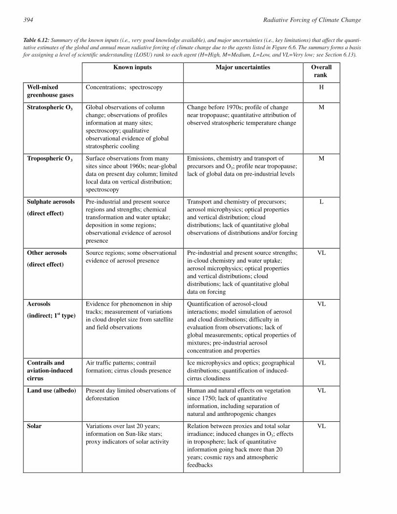
394 Radiative Forcing of Climate Change
Table 6.12: Summary of the known inputs (i.e., very good knowledge available), and major uncertainties (i.e., key limitations) that affect the quanti-tative estimates of the global and annual mean radiative forcing of climate change due to the agents listed in Figure 6.6. The summary forms a basisfor assigning a level of scientific understanding (LOSU) rank to each agent (H=High, M=Medium, L=Low, and VL=Very low; see Section 6.13).
Known inputs Major uncertainties Overallrank
Well-mixedgreenhouse gases
Concentrations; spectroscopy H
Stratospheric O3 Global observations of columnchange; observations of profilesinformation at many sites;spectroscopy; qualitativeobservational evidence of globalstratospheric cooling
Change before 1970s; profile of changenear tropopause; quantitative attribution ofobserved stratospheric temperature change
M
Tropospheric O3 Surface observations from manysites since about 1960s; near-globaldata on present day column; limitedlocal data on vertical distribution;spectroscopy
Emissions, chemistry and transport ofprecursors and O3; profile near tropopause;lack of global data on pre-industrial levels
M
Sulphate aerosols
(direct effect)
Pre-industrial and present sourceregions and strengths; chemicaltransformation and water uptake;deposition in some regions;observational evidence of aerosolpresence
Transport and chemistry of precursors;aerosol microphysics; optical propertiesand vertical distribution; clouddistributions; lack of quantitative globalobservations of distributions and/or forcing
L
Other aerosols
(direct effect)
Source regions; some observationalevidence of aerosol presence
Pre-industrial and present source strengths;in-cloud chemistry and water uptake;aerosol microphysics; optical propertiesand vertical distributions; clouddistributions; lack of quantitative globaldata on forcing
VL
Aerosols
(indirect; 1st type)
Evidence for phenomenon in shiptracks; measurement of variationsin cloud droplet size from satelliteand field observations
Quantification of aerosol-cloudinteractions; model simulation of aerosoland cloud distributions; difficulty inevaluation from observations; lack ofglobal measurements; optical properties ofmixtures; pre-industrial aerosolconcentration and properties
VL
Contrails andaviation-inducedcirrus
Air traffic patterns; contrailformation; cirrus clouds presence
Ice microphysics and optics; geographicaldistributions; quantification of induced-cirrus cloudiness
VL
Land use (albedo) Present day limited observations ofdeforestation
Human and natural effects on vegetationsince 1750; lack of quantitativeinformation, including separation ofnatural and anthropogenic changes
VL
Solar Variations over last 20 years;information on Sun-like stars;proxy indicators of solar activity
Relation between proxies and total solarirradiance; induced changes in O3; effectsin troposphere; lack of quantitativeinformation going back more than 20years; cosmic rays and atmosphericfeedbacks
VL

accorded for tropospheric O3 forcing. Key uncertainties remainconcerning the pre-industrial distributions, the effects of stratos-pheric-tropospheric exchange and the manner of its evolutionover time, as well as the seasonal cycle in some regions of theglobe.
As the LOSU rankings are subjective and reflect qualitativeconsiderations, the fact that tropospheric and stratospheric O3
have the same ranks does not imply that the degree of confidencein their respective estimates is identical. In fact, from the observa-tional standpoint, stratospheric O3 forcing, which has occurredonly since 1970s and is better documented, is on relatively firmerground. Nevertheless, both O3 components are less certain relativeto the well-mixed greenhouse gases, but more so compared withthe agents discussed below.
The estimate for the direct sulphate aerosol forcing has alsoseen multiple model investigations since the SAR, resulting inmore estimates being available for this assessment. It is strikingthat consideration of all of the estimates available since 1996 leadto the same best estimate (–0.4 Wm−2) and uncertainty (–0.2 to–0.8 Wm−2) range as in the previous assessment. As in the case ofO3, that could be a motivation for elevating the status ofknowledge of this forcing to a higher confidence level. However,there remain critical areas of uncertainty concerning themodelling of the geographical distribution of sulphate aerosols,spatial cloud distributions, effects due to relative humidity etc.Hence, we retain a “low” LOSU for this forcing.
The SAR stated a radiative forcing of +0.1 Wm−2 for fossilfuel (FF) black carbon aerosols with a range +0.03 to +0.3 Wm−2,and a “very low” level of confidence. For biomass burning (BB)aerosols, the SAR stated a radiative forcing of −0.2 Wm−2 with arange −0.07 to −0.6 Wm−2, and a “very low” level of confidence.In the present assessment, the radiative forcing of the black carboncomponent from FF is estimated to be +0.2 Wm−2 with a rangefrom +0.1 to +0.4 Wm−2 based on studies since the SAR. A “verylow” LOSU is accorded in view of the differences in the estimatesfrom the various models. The organic carbon component from FFis estimated to yield a forcing of –0.1 Wm−2 with a range from–0.03 to –0.30 Wm−2; this has a “very low” LOSU. Note thatextreme caution must be exercised in adding the uncertainties ofthe organic and black carbon components to get the uncertaintyfor FF as a whole. For BB aerosols, no attempt is made to separateinto black and organic carbon components, in view of consider-able uncertainties. The central estimate and range for BB aerosolsremains the same as in the SAR; this has a “very low” LOSU inview of the several uncertainties in the calculations (Section 6.7).
Mineral dust is a new component in the current assessment.The studies on the “disturbed” soils suggest an anthropogenicinfluence, with a range from +0.4 to −0.6 Wm−2. In general, theevaluation for dust aerosol is complicated by the fact that theshort-wave consists of a significant reflection and absorptioncomponent, and the long-wave also exerts a substantial contribu-tion by way of a trapping of the infrared radiation. Thus, the netradiative energy gained or lost by the system is the differencebetween non-negligible positive and negative radiative fluxchanges operating simultaneously. Because of this complexity,we refrain from giving a best estimate and accord this componenta “very low” LOSU.
As explained in Section 6.8, the “indirect” forcing due to alltropospheric aerosols can be thought of as comprising twoeffects. Only the first type of effect as applicable in the context ofliquid clouds is considered here. As in the SAR, no best estimateis given in view of the large uncertainties prevailing in thisproblem (Section 6.8). The range (0 to −2 Wm−2) is based onpublished estimates and subjective assessment of the uncertain-ties. Although several model studies suggest a non-zero, negativevalue as the upper bound (about −0.3 Wm−2), substantial gaps inthe knowledge remain which affect the confidence in the modelsimulations of this forcing (e.g., uncertainties in aerosol andcloud processes and their representations in GCMs, thepotentially incomplete knowledge of the radiative effect of blackcarbon in clouds, and the possibility that the forcings forindividual aerosol types may not be additive), such that thepossibility of a very small negative value cannot be excluded;thus zero is retained as an upper bound as in the SAR. In view ofthe large uncertainties in the processes and the quantification, a“very low” LOSU is assigned to this forcing. Inclusion of thesecond indirect effect (Chapter 5) is fraught with even moreuncertainties and, despite being conceptually valid as an anthro-pogenic perturbation, raises the question of whether the modelestimates to-date can be unambiguously characterised as anaerosol radiative forcing.
Aviation introduces two distinct types of perturbation(Section 6.8). Contrails produced by aircraft constitute ananthropogenic perturbation. This is estimated to contribute 0.02Wm−2 with an uncertainty of a factor of 3 or 4 (IPCC, 1999); theuncertainty factor is assumed to be 3.5 in Figure 6.6. This has anextremely low level of confidence associated with it.Additionally, aviation-produced cirrus is estimated by IPCC(1999) to yield a forcing of 0 to 0.04 Wm−2, but no centralestimate or uncertainty range was estimated in that report. Bothcomponents have a “very low” LOSU.
Volcanic aerosols that represent a transient forcing of theclimate system following an eruption are not plotted since they areepisodic events and cannot be categorised as a century-scalesecular forcing, unlike the others. However, they can havesubstantial impacts on interannual to decadal scale temperaturechanges and hence are important factors in the time evolution ofthe forcing (see Section 6.15). Some studies (Hansen et al., 1998;Shine and Forster, 1999) have attempted to scale the volcanicforcings in a particular decade with respect to that in a quiescentdecade.
Land-use change was dealt with in IPCC (1990) but was notconsidered in the SAR. However, recent studies (e.g., Hansen etal., 1998) have raised the possibility of a negative forcing due todeforestation and the ensuing effects of snow-covered land albedochanges in mid-latitudes. There are not many studies on thissubject and rigorous investigations are lacking such that thisforcing has a “very low” LOSU, with the range in the estimatebeing 0 to –0.4 Wm−2 (central estimate: −0.2 Wm−2). Note that theland-use forcing here is restricted to that due to albedo change.
Solar forcing remains the same as in the SAR, in terms of bestestimate, the uncertainty range and the confidence level. Thus, therange is 0.1 to 0.5 Wm−2 with a best estimate of 0.3 Wm−2, andwith a “very low” LOSU.
395Radiative Forcing of Climate Change

6.13.2 Limitations
It is important that the global mean forcing estimates beinterpreted in a proper manner. Recall that the utility of theforcing concept is to afford a first-order perspective into therelative climatic impacts (viz., global-mean surface temperaturechange) of the different forcings. As stated in Section 6.2, formany of the relevant forcings (e.g., well-mixed greenhouse gases,solar, certain aerosol and O3 profile cases), model studies suggesta reasonable similarity of the climate sensitivity factor (Equation6.1), such that a comparison of these forcings is meaningful forassessing their relative effects on the global mean surface temper-ature. However, as mentioned earlier, the climate sensitivityfactor for some of the spatially inhomogeneous forcings has yetto be fully explored. For some of the forcings (e.g., involvingsome absorbing aerosol and O3 profile cases; see Hansen et al.,1997a), the climate sensitivity is markedly different than for, say,the well-mixed greenhouse gases, while, for other forcings (e.g.,indirect aerosol effect), more comprehensive studies are neededbefore a generalisation can become possible.
It is also cautioned that it may be inappropriate to perform asum of the forcings to derive a best estimate “total” radiativeforcing. Such an operation has the limitation that there arediffering degrees of reliability of the global mean estimates of thevarious forcings, which do not necessarily lend themselves to awell-justified quantitative manipulation. For some forcings, thereis not even a central or best estimate given at present (e.g.,indirect aerosol forcing), essentially due to the substantialuncertainties.
The ranges given for the various forcings in Figure 6.6, asalready pointed out, do not have a statistical basis and are guidedmostly by the estimates from published model studies.Performing mathematical manipulations using these ranges toobtain a “net uncertainty range” for the total forcing, therefore,lacks a rigorous basis. Adding to the complexity is the fact thateach forcing has associated with it an assessment of the level ofknowledge that is subjective in nature viz., LOSU (Table 6.12).The LOSU index is not a quantitative indicator and, at best, yieldsa qualitative sense about the reliability of the estimates, with thewell-mixed greenhouse gases having the highest reliability, thosewith “medium” rank having lesser reliability, and with even lessreliability for the “low” and “very low” rankings. To some extent,the relatively lower ranking of the non-well-mixed greenhousegases (e.g., aerosols, O3) is associated with the fact that theforcing estimates for these agents depend on model simulationsof species’ concentrations, in contrast to the well-mixedgreenhouse gases whose global concentrations are well quanti-fied.
In a general sense, the strategy and usefulness of combiningglobal mean estimates of forcings that have different signs,spatial patterns, vertical structures, uncertainties, and LOSUs,and the resulting significance in the context of the global climateresponse are yet to be fully explored. For some combinations offorcing agents (e.g., well-mixed greenhouse gases and sulphateaerosol; see Section 6.2), it is apparent from model tests that theglobal mean responses to the individual forcings can be added toyield the total global mean response. Because linear additivity
tests have yet to be performed for the complete set of agentsshown in Figure 6.6, it is not possible to state with absolutecertainty that the additivity concept will necessarily hold for theentire set of forcings.
Figure 6.6 depicts the uncertainties and LOSUs only for theglobal mean estimates. No attempt is made here to extend thesesubjective characterisations to the spatial domains associatedwith each of the forcings (see Figure 6.7, and Table 6.11 for theNorthern to Southern Hemisphere ratios). As in the SAR, wereiterate that, in view of the spatial character of several of theforcing agents, the global mean estimates do not necessarilydescribe the complete spatial (horizontal and verticaldimensions) and seasonal climate responses to a particularradiative perturbation. Nor do they yield quantitative informationabout changes in parameters other than the global mean surfacetemperature response.
One diagnostic constraint on the total global mean forcingsince pre-industrial times is likely to be provided by comparisonsof model-simulated (driven by the combination of forcings) andobserved climate changes, including spatially-based detection-attribution analyses (Chapter 12). However, the a posterioriinference involves a number of crucial assumptions, including theuncertainties associated with the forcings, the representativenessof the climate models’ sensitivity to the forcings, and the model’srepresentation of the real world’s “natural” variations.
Overall, the net forcing comprises of a large positive valuedue to well-mixed greenhouse gases, followed by a number ofother agents that have smaller positive or negative values. Thus,relative to IPCC (1990) and over this past decade, there are nowmore forcing agents to be accounted for, each with a sizeableuncertainty that can affect the estimated climate response. In thisregard, consideration of the “newer” forcing agents brings on anadditional element of uncertainty in climate change analyses,over and above those concerning climate feedbacks and naturalvariability (IPCC, 1990). Both the spatial character of the forcingand doubts about the magnitudes (and, in some cases, even thesign) add to the complexity of the climate change problem.However, this does not necessarily imply that the uncertaintyassociated with the forcings is now of much greater importancethan the issue of climate sensitivity of models.
6.14 The Geographical Distribution of the Radiative Forcings
While previous sections have concentrated upon estimates of theglobal annual mean of the radiative forcing of particularmechanisms, this section presents the geographical distributionof the present day radiative forcings. Although the exact spatialdistribution of the radiative forcing may differ between studies,many of them show similar features that are highlighted in thissection. With the exception of well-mixed greenhouse gases,different studies calculate different magnitudes of the radiativeforcing. In these cases, the spatial distributions are discussed, notthe absolute values of the radiative forcing. It should be stressedthat the Figure 6.7 represents plausible examples of geographicaldistributions only – significant differences may occur in otherstudies. In addition to Figure 6.7, Table 6.11 lists Northern toSouthern Hemisphere ratio for forcings.
396 Radiative Forcing of Climate Change
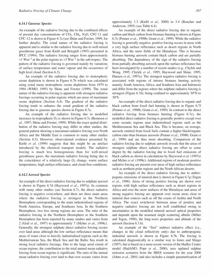
6.14.1 Gaseous Species
An example of the radiative forcing due to the combined effectsof present day concentrations of CO2, CH4, N2O, CFC-11 andCFC-12 is shown in Figure 6.7a (see Shine and Forster, 1999, forfurther details). The zonal nature of the radiative forcing isapparent and is similar to the radiative forcing due to well-mixedgreenhouse gases from Kiehl and Briegleb (1993) presented inIPCC (1994). The radiative forcing ranges from approximately+1 Wm−2 at the polar regions to +3 Wm−2 in the sub-tropics. Thepattern of the radiative forcing is governed mainly by variationsof surface temperature and water vapour and the occurrence ofhigh level cloud (Section 6.3).
An example of the radiative forcing due to stratosphericozone depletion is shown in Figure 6.7b which was calculatedusing zonal mean stratospheric ozone depletions from 1979 to1994 (WMO, 1995) by Shine and Forster (1999). The zonalnature of the radiative forcing is apparent with strongest radiativeforcings occurring in polar regions which are areas of maximumozone depletion (Section 6.4). The gradient of the radiativeforcing tends to enhance the zonal gradient of the radiativeforcing due to gaseous species shown in Figure 6.7a.
An example of the radiative forcing due to modelledincreases in tropospheric O3 is shown in Figure 6.7c (Berntsen etal., 1997; Shine and Forster, 1999). While the exact spatial distri-bution of the radiative forcing may differ in other studies, thegeneral pattern showing a maximum radiative forcing over NorthAfrica and the Middle East is common to many other studies(Section 6.5). However, observational evidence presented byKiehl et al. (1999) suggests that this might be an artefactintroduced by the chemical transport models. The radiativeforcing is much less homogeneous than for well-mixedgreenhouse gases, the maximum radiative forcing being due tothe coincidence of a relatively large O3 change, warm surfacetemperatures, high surface reflectance, and cloud-free conditions.
6.14.2 Aerosol Species
An example of the direct radiative forcing due to sulphate aerosolis shown in Figure 6.7d (Haywood et al., 1997a). In commonwith many other studies (see Section 6.7), the direct radiativeforcing is negative everywhere, and there are three main areaswhere the radiative forcing is strongest in the NorthernHemisphere corresponding to the main industrialised regions ofNorth America, Europe, and Southeast Asia. In the SouthernHemisphere, two less strong regions are seen. The ratio of theradiative forcing in the Northern Hemisphere to the SouthernHemisphere has been reported by many studies and varies from2 (Graf et al., 1997) to approximately 7 (Myhre et al., 1998c).Generally, the strongest sulphate direct radiative forcing occursover land areas although the low surface reflectance means thatareas of water close to heavily industrialised regions such as theMediterranean Sea, the Black Sea and the Baltic Sea result instrong local radiative forcings. Due to the large areal extent ofocean regions, the contribution to the total annual mean radiativeforcing from ocean regions is significant. The ratio of the annualmean radiative forcing over land to that over oceans varies from
approximately 1.3 (Kiehl et al., 2000) to 3.4 (Boucher andAnderson, 1995) (see Table 6.4).
An example of the direct radiative forcing due to organiccarbon and black carbon from biomass burning is shown in Figure6.7e (Penner et al., 1998b; Grant et al., 1999). While the radiativeforcing is generally negative, positive forcing occurs in areas witha very high surface reflectance such as desert regions in NorthAfrica, and the snow fields of the Himalayas. This is becausebiomass burning aerosols contain black carbon and are partiallyabsorbing. The dependency of the sign of the radiative forcingfrom partially absorbing aerosols upon the surface reflectance hasbeen investigated by a number of recent studies (e.g., Chylek andWong, 1995; Chylek et al., 1995; Haywood and Shine, 1995;Hansen et al., 1997a). The strongest negative radiative forcing isassociated with regions of intense biomass burning activitynamely, South America, Africa, and Southern Asia and Indonesiaand differ from the regions where the sulphate radiative forcing isstrongest (Figure 6.7d), being confined to approximately 30oN to30oS.
An example of the direct radiative forcing due to organic andblack carbon from fossil fuel burning is shown in Figure 6.7f(Penner et al., 1998b; Grant et al., 1999). In contrast to the directradiative forcing from biomass burning (Figure 6.7e), themodelled direct radiative forcing is generally positive except oversome oceanic regions near industrialised regions such as theMediterranean Sea and Black Sea. This is because, on average,aerosols emitted from fossil fuels contain a higher black/organiccarbon ratio than biomass aerosols (Penner et al., 1998b; Grant etal., 1999) and are thus more absorbing. Comparison of theradiative forcing due to sulphate aerosols reveals that the areas ofstrongest sulphate direct radiative forcing are offset to somedegree by the radiative forcing due to fossil fuel emissions ofblack carbon as shown in calculations by Haywood et al. (1997a)and Myhre et al. (1998c). Additional regions of moderate positiveradiative forcing are present over areas of high surface reflectancesuch as northern polar regions and the North African deserts.
An example of the direct radiative forcing due to anthro-pogenic emissions of mineral dust is shown in Figure 6.7g (Tegenet al., 1996). Areas of strong positive forcing are shown overregions with high surface reflectance such as desert regions inAfrica and over the snow surfaces of the Himalayas and areas ofstrong negative forcing are apparent over ocean areas close tomineral dust sources such as off the coasts of Arabia and NorthAfrica. The exact switchover between areas of positive andnegative radiative forcing are not well established owing touncertainties in the modelled mineral aerosol optical propertiesand depends upon the assumed single scattering albedo (Millerand Tegen, 1998), the long-wave properties and altitude of theaerosol (Section 6.7.6).
An example of the “first” indirect radiative effect (i.e.,changes in the cloud reflectivity only) due to anthropogenicindustrial aerosols is shown in Figure 6.7h. The forcing iscalculated diagnostically in a similar way to Jones and Slingo(1997), but is based on a more recent version of the Hadley Centremodel (HadAM3; Pope et al., 2000), uses updated sulphuremission scenarios from the SRES scenario for the year 2000(Johns et al., 2001) and also includes a simple parametrization of
397Radiative Forcing of Climate Change
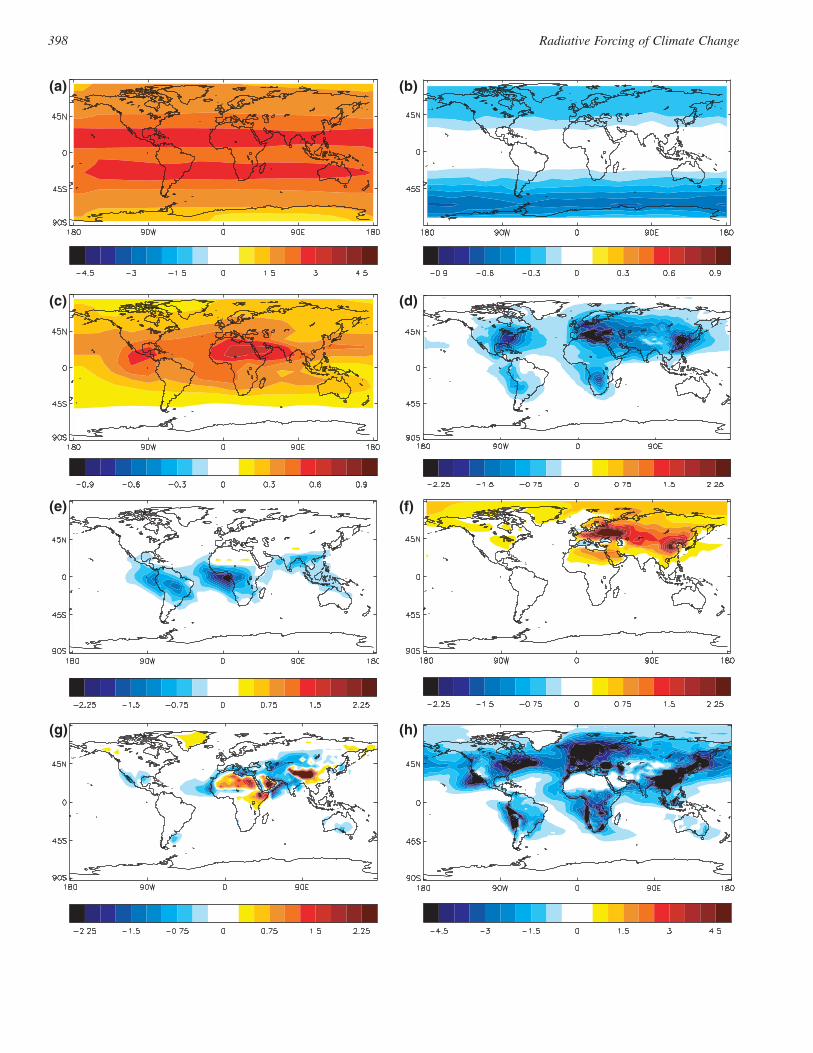
398 Radiative Forcing of Climate Change
(a) (b)
(c) (d)
(e) (f)
(g) (h)
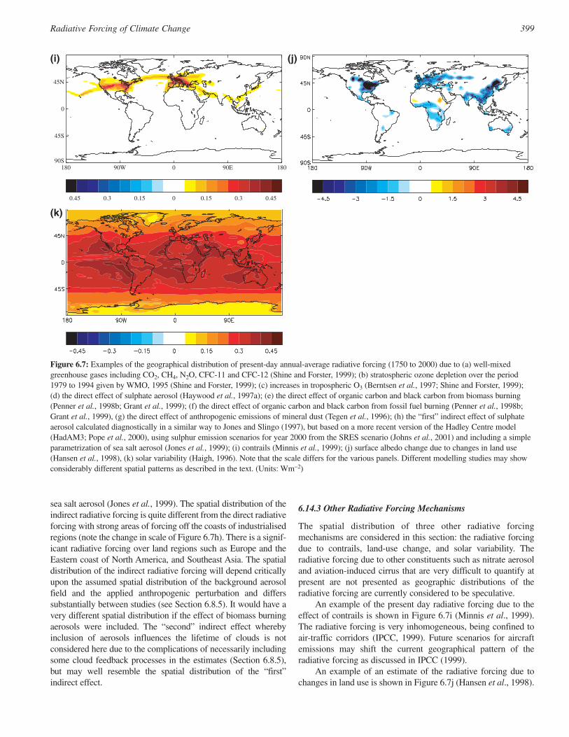
sea salt aerosol (Jones et al., 1999). The spatial distribution of theindirect radiative forcing is quite different from the direct radiativeforcing with strong areas of forcing off the coasts of industrialisedregions (note the change in scale of Figure 6.7h). There is a signif-icant radiative forcing over land regions such as Europe and theEastern coast of North America, and Southeast Asia. The spatialdistribution of the indirect radiative forcing will depend criticallyupon the assumed spatial distribution of the background aerosolfield and the applied anthropogenic perturbation and differssubstantially between studies (see Section 6.8.5). It would have avery different spatial distribution if the effect of biomass burningaerosols were included. The “second” indirect effect wherebyinclusion of aerosols influences the lifetime of clouds is notconsidered here due to the complications of necessarily includingsome cloud feedback processes in the estimates (Section 6.8.5),but may well resemble the spatial distribution of the “first”indirect effect.
6.14.3 Other Radiative Forcing Mechanisms
The spatial distribution of three other radiative forcingmechanisms are considered in this section: the radiative forcingdue to contrails, land-use change, and solar variability. Theradiative forcing due to other constituents such as nitrate aerosoland aviation-induced cirrus that are very difficult to quantify atpresent are not presented as geographic distributions of theradiative forcing are currently considered to be speculative.
An example of the present day radiative forcing due to theeffect of contrails is shown in Figure 6.7i (Minnis et al., 1999).The radiative forcing is very inhomogeneous, being confined toair-traffic corridors (IPCC, 1999). Future scenarios for aircraftemissions may shift the current geographical pattern of theradiative forcing as discussed in IPCC (1999).
An example of an estimate of the radiative forcing due tochanges in land use is shown in Figure 6.7j (Hansen et al., 1998).
399Radiative Forcing of Climate Change
180 90W 0 90E 18090S
45S
0
45N
0.45 0.3 0.15 0 0.15 0.3 0.45
(i)
(k)
(j)
Figure 6.7: Examples of the geographical distribution of present-day annual-average radiative forcing (1750 to 2000) due to (a) well-mixedgreenhouse gases including CO2, CH4, N2O, CFC-11 and CFC-12 (Shine and Forster, 1999); (b) stratospheric ozone depletion over the period1979 to 1994 given by WMO, 1995 (Shine and Forster, 1999); (c) increases in tropospheric O3 (Berntsen et al., 1997; Shine and Forster, 1999);(d) the direct effect of sulphate aerosol (Haywood et al., 1997a); (e) the direct effect of organic carbon and black carbon from biomass burning(Penner et al., 1998b; Grant et al., 1999); (f) the direct effect of organic carbon and black carbon from fossil fuel burning (Penner et al., 1998b;Grant et al., 1999), (g) the direct effect of anthropogenic emissions of mineral dust (Tegen et al., 1996); (h) the “first” indirect effect of sulphateaerosol calculated diagnostically in a similar way to Jones and Slingo (1997), but based on a more recent version of the Hadley Centre model(HadAM3; Pope et al., 2000), using sulphur emission scenarios for year 2000 from the SRES scenario (Johns et al., 2001) and including a simpleparametrization of sea salt aerosol (Jones et al., 1999); (i) contrails (Minnis et al., 1999); (j) surface albedo change due to changes in land use(Hansen et al., 1998), (k) solar variability (Haigh, 1996). Note that the scale differs for the various panels. Different modelling studies may showconsiderably different spatial patterns as described in the text. (Units: Wm−2)

The areas of strongest negative forcing occur at northern latitudesof the Northern Hemisphere due to the felling of forests whichhave a lower albedo when snow is present (see Section 6.13).Additional effects are due to the change in albedo between croplands and naturally occurring vegetation. Examples where theradiative forcing is positive include areas where irrigation hasenabled crop-growing on previously barren land.
An example of the present day radiative forcing due to solarvariability is shown in Figure 6.7k. The solar radiative forcingwas calculated by scaling the top of the atmosphere net solarradiation such that the global average is +0.3 Wm−2 (as deducedfor global average radiative forcing since 1750, see Section6.13.1). Thus it assumes a 0.125% increase in solar constant andno change in any other parameter (e.g., O3, cloud). The cloud andradiation fields were calculated within a run of the UGAMPGCM (Haigh, 1996). The strongest radiative forcings exist wherethe surface reflectance is low (i.e., oceanic regions) and theinsolation is highest (i.e., equatorial regions). The solar radiativeforcing is also modulated by cloud amount, areas with low cloudamount showing the strongest radiative forcing. The solarradiative forcing is more inhomogeneous than the radiativeforcing due to gaseous species (Section 6.14.1), but morehomogeneous than the radiative forcing due to aerosol species(Section 6.14.2).
While the preceding sections have shown that the radiativeforcing due to the different forcing mechanisms have verydifferent spatial distributions, it is essential to note that theforcing/response relationship given in Section 6.2 relates globalmean radiative forcings to global mean temperature response.Thus, it is not possible to simply map the geographical radiativeforcing mechanisms by assuming a globally invariant climatesensitivity parameter to predict a geographic temperatureresponse, due to the complex nature of the atmosphere-oceansystem. Rather, the effects of spatial inhomogeneity in the distri-bution of the radiative forcing may lead to locally differentresponses in surface temperature (Section 6.2) indicating that thespatial distributions of the radiative forcing need to be accuratelyrepresented to improve regional estimates of surface temperatureresponse and other physical parameters.
6.15 Time Evolution of Radiative Forcings
6.15.1 Past to Present
IPCC (1990) showed time evolution of the radiative forcing dueto the well-mixed greenhouse gases. For the other radiativeforcing mechanisms, the previous IPCC reports (IPCC, 1990;SAR) did not consider the evolution of the radiative forcing, andassessed mainly the radiative fluxes in the pre-industrial andpresent epochs. However, more recent studies have consideredthe time evolution of several forcing mechanisms (Hansen et al.,1993; Wigley et al., 1997; Myhre et al., 2001). The informationon the time evolution of the radiative forcing from pre-industrialtimes to present illustrates the differing importance of the variousradiative forcing mechanisms over the various time periods, aswell as the different start times of their perturbation of theradiative balance. It also gives useful information in the form of
inputs to climate models viz., as driving mechanisms to investi-gate potential causes of climate changes. Studies of the evolutionof various anthropogenic as well as natural forcing mechanismsmay then be used to explain potential causes of past climatechange, e.g. since pre-industrial times (Chapter 12).
The knowledge of the various forcing mechanisms variessubstantially (see Section 6.13) and, for some, the knowledge oftheir time evolution is more problematic than for others. Forexample, well-mixed greenhouse gas concentrations areobserved very accurately from about 1950, with observationseven further back in time, whereas data for most aerosolcomponents are much more scarce and uncertain. Uncertaintiesin the evolution of many of the radiative forcing mechanismsshown in Figure 6.8 have not been assessed yet, and the presentedtime history should be regarded as an example of a possibleevolution.
The forcing mechanisms, considered, where information ontheir time evolution is available, are plotted in Figure 6.8, withthe present forcing corresponding to the best estimates given inSection 6.13. The time evolution differs considerably among theforcing mechanisms as different processes controlling theemissions and lifetimes are involved. Concentrations of the well-mixed greenhouse gases are taken from Chapters 3 and 4 and thesimplified expressions for the radiative forcing in Table 6.2 (firstrow for CO2) are used. The evolution of the radiative forcing dueto tropospheric O3 is taken from Berntsen et al. (2000). For theradiative forcing due to stratospheric O3, information on theevolution is taken from the SAR and scaled to the present forcingof −0.15 Wm−2 (Section 6.4).
For sulphate, the time evolution for SO2 emission(Schlesinger et al., 1992) is used, updated with values after 1990(Stern and Kaufmann, 1996). For black and organic carbonaerosols, the fossil fuel component is scaled to coal, diesel, andoil use and fossil fuel emission (IPCC, 1996b), respectively.Altered emission coefficients as a result of improved technologyhave not been taken into account and is a substantial uncertaintyfor the time evolution of the black carbon emission. The biomasscomponent is scaled to the gross deforestation (see SAR). Inaddition to different forcing mechanisms of anthropogenic origin,two natural forcings have also been considered: solar irradiancevariations and stratospheric aerosols of volcanic origin. The Leanet al. (1995) and Hoyt and Schatten (1993) estimates of directsolar forcing due to variation in total solar irradiance are shown.Differences between the solar irradiance constructions are due touse of different proxy parameters for the solar irradiancevariations (Section 6.11). The optical depth of the stratosphericaerosols of volcanic origin is taken from Sato et al. (1993) andRobock and Free (1996). The data from Sato et al. (1993)(updated from www.giss.nasa.gov) are given for the period 1850to 1998, whereas those from Robock and Free (1996) are for theperiod 1750 to 1988. In Robock and Free (1996) the optical depthis given for the Northern Hemisphere. The relationship betweenoptical depth and radiative forcing from Lacis et al. (1992) isused. The stratospheric aerosols yield a very strong forcingimmediately after major eruptions (Section 6.9); however, thelifetime of the stratospheric aerosols is only a few years. Therefore,the transient response due to the forcing by stratospheric aerosols
400 Radiative Forcing of Climate Change
cannot readily be compared to that due to the more sustained orsteadily increasing forcings.
The relative evolution of the strengths of the different forcingmechanisms presented above are seen to be very different. Theforcing due to well-mixed greenhouse gases (consisting of thecomponents listed in Table 6.11) is the dominant forcingmechanism over the century time period. For tropospheric O3, therelative radiative forcing compared to the well-mixed greenhousegases has slightly increased; it was 10% of the well-mixedgreenhouse gas forcing in 1900 and is 15% at present. Thestratospheric O3 forcing is significant only over the last two
decades. The aerosols have short lifetimes compared with thewell-mixed greenhouse gases, and their forcings at any giventime depend on the current emissions. This is not the case for thewell-mixed greenhouse gases for which both current andprevious emissions are relevant. Table 6.13 shows five yearaverages for the radiative forcings denoted in Figure 6.8 over theperiod 1960 to 1995. For some of the forcing mechanisms a largeincrease in the radiative forcing (computed since pre-industrialtimes) is estimated to have occurred over the period 1960 to1995. This is the case for the well-mixed greenhouse gases,tropospheric O3, biomass burning aerosols and organic carbon
401Radiative Forcing of Climate Change
(c) (d)
(a) (b)R
adia
tive
forc
ing
(Wm
−2)
Rad
iativ
e fo
rcin
g (W
m−2
)
Rad
iativ
e fo
rcin
g (W
m−2
)R
adia
tive
forc
ing
(Wm
−2)
Figure 6.8: Time evolution of global mean radiative forcing from pre-industrial times (1750) to present. Annual mean radiative forcing values areshown, except for stratospheric aerosols of volcanic origin where a three-year running mean is used. Radiative forcings due to (a) well-mixedgreenhouse gases, tropospheric O3, and stratospheric O3, (b) direct effect of sulphate aerosols, fossil fuel organic and black carbon aerosols, andbiomass burning aerosols, (c) solar irradiance variations from Lean et al. (1995) and Hoyt and Schatten (1993), respectively, and (d) stratosphericaerosols of volcanic origin from Sato et al. (1993) (and updated with data from www.giss.nasa.gov) for the period 1850 to 1998 and from Robockand Free (1996) for the period 1750 to 1988 (for the Northern Hemisphere only). Note the change of scales in the different panels.
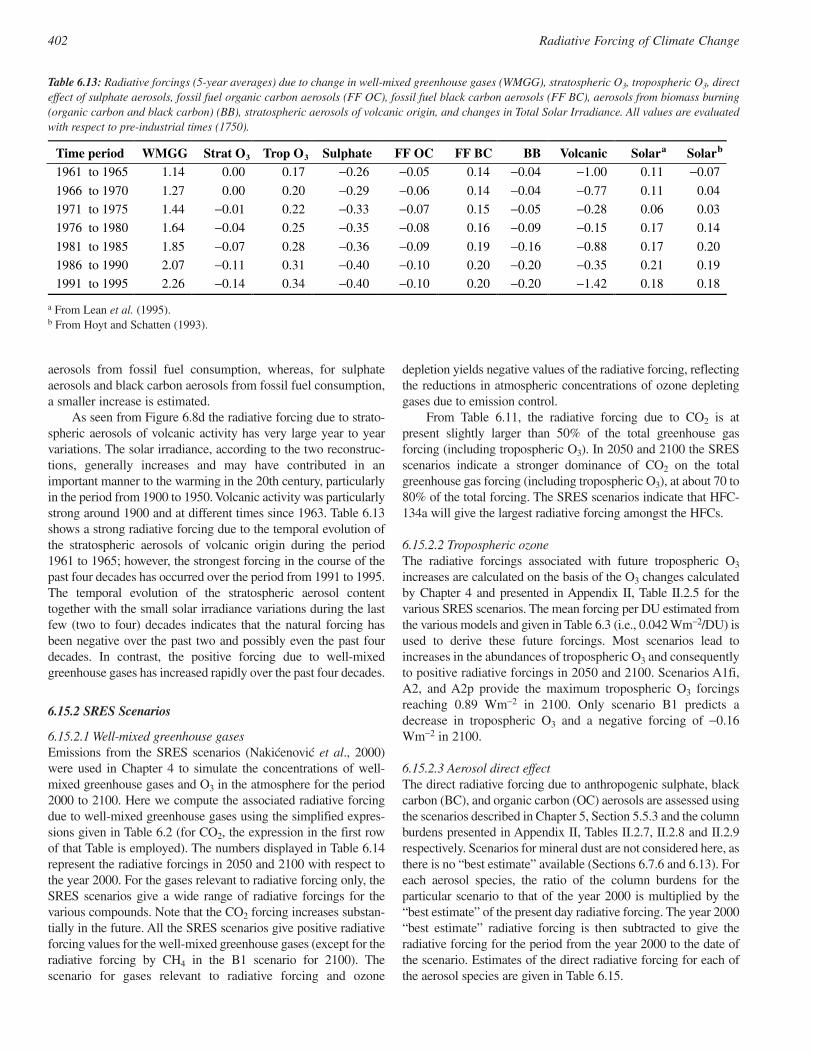
aerosols from fossil fuel consumption, whereas, for sulphateaerosols and black carbon aerosols from fossil fuel consumption,a smaller increase is estimated.
As seen from Figure 6.8d the radiative forcing due to strato-spheric aerosols of volcanic activity has very large year to yearvariations. The solar irradiance, according to the two reconstruc-tions, generally increases and may have contributed in animportant manner to the warming in the 20th century, particularlyin the period from 1900 to 1950. Volcanic activity was particularlystrong around 1900 and at different times since 1963. Table 6.13shows a strong radiative forcing due to the temporal evolution ofthe stratospheric aerosols of volcanic origin during the period1961 to 1965; however, the strongest forcing in the course of thepast four decades has occurred over the period from 1991 to 1995.The temporal evolution of the stratospheric aerosol contenttogether with the small solar irradiance variations during the lastfew (two to four) decades indicates that the natural forcing hasbeen negative over the past two and possibly even the past fourdecades. In contrast, the positive forcing due to well-mixedgreenhouse gases has increased rapidly over the past four decades.
6.15.2 SRES Scenarios
6.15.2.1 Well-mixed greenhouse gasesEmissions from the SRES scenarios (Nakicenovic et al., 2000)were used in Chapter 4 to simulate the concentrations of well-mixed greenhouse gases and O3 in the atmosphere for the period2000 to 2100. Here we compute the associated radiative forcingdue to well-mixed greenhouse gases using the simplified expres-sions given in Table 6.2 (for CO2, the expression in the first rowof that Table is employed). The numbers displayed in Table 6.14represent the radiative forcings in 2050 and 2100 with respect tothe year 2000. For the gases relevant to radiative forcing only, theSRES scenarios give a wide range of radiative forcings for thevarious compounds. Note that the CO2 forcing increases substan-tially in the future. All the SRES scenarios give positive radiativeforcing values for the well-mixed greenhouse gases (except for theradiative forcing by CH4 in the B1 scenario for 2100). Thescenario for gases relevant to radiative forcing and ozone
depletion yields negative values of the radiative forcing, reflectingthe reductions in atmospheric concentrations of ozone depletinggases due to emission control.
From Table 6.11, the radiative forcing due to CO2 is atpresent slightly larger than 50% of the total greenhouse gasforcing (including tropospheric O3). In 2050 and 2100 the SRESscenarios indicate a stronger dominance of CO2 on the totalgreenhouse gas forcing (including tropospheric O3), at about 70 to80% of the total forcing. The SRES scenarios indicate that HFC-134a will give the largest radiative forcing amongst the HFCs.
6.15.2.2 Tropospheric ozoneThe radiative forcings associated with future tropospheric O3
increases are calculated on the basis of the O3 changes calculatedby Chapter 4 and presented in Appendix II, Table II.2.5 for thevarious SRES scenarios. The mean forcing per DU estimated fromthe various models and given in Table 6.3 (i.e., 0.042 Wm−2/DU) isused to derive these future forcings. Most scenarios lead toincreases in the abundances of tropospheric O3 and consequentlyto positive radiative forcings in 2050 and 2100. Scenarios A1fi,A2, and A2p provide the maximum tropospheric O3 forcingsreaching 0.89 Wm−2 in 2100. Only scenario B1 predicts adecrease in tropospheric O3 and a negative forcing of −0.16Wm−2 in 2100.
6.15.2.3 Aerosol direct effectThe direct radiative forcing due to anthropogenic sulphate, blackcarbon (BC), and organic carbon (OC) aerosols are assessed usingthe scenarios described in Chapter 5, Section 5.5.3 and the columnburdens presented in Appendix II, Tables II.2.7, II.2.8 and II.2.9respectively. Scenarios for mineral dust are not considered here, asthere is no “best estimate” available (Sections 6.7.6 and 6.13). Foreach aerosol species, the ratio of the column burdens for theparticular scenario to that of the year 2000 is multiplied by the“best estimate” of the present day radiative forcing. The year 2000“best estimate” radiative forcing is then subtracted to give theradiative forcing for the period from the year 2000 to the date ofthe scenario. Estimates of the direct radiative forcing for each ofthe aerosol species are given in Table 6.15.
402 Radiative Forcing of Climate Change
Time period WMGG Strat O3 Trop O3 Sulphate FF OC FF BC BB Volcanic Solara Solarb
1961 to 1965 1.14 0.00 0.17 −0.26 −0.05 0.14 −0.04 −1.00 0.11 −0.07
1966 to 1970 1.27 0.00 0.20 −0.29 −0.06 0.14 −0.04 −0.77 0.11 0.04
1971 to 1975 1.44 −0.01 0.22 −0.33 −0.07 0.15 −0.05 −0.28 0.06 0.03
1976 to 1980 1.64 −0.04 0.25 −0.35 −0.08 0.16 −0.09 −0.15 0.17 0.14
1981 to 1985 1.85 −0.07 0.28 −0.36 −0.09 0.19 −0.16 −0.88 0.17 0.20
1986 to 1990 2.07 −0.11 0.31 −0.40 −0.10 0.20 −0.20 −0.35 0.21 0.19
1991 to 1995 2.26 −0.14 0.34 −0.40 −0.10 0.20 −0.20 −1.42 0.18 0.18
Table 6.13: Radiative forcings (5-year averages) due to change in well-mixed greenhouse gases (WMGG), stratospheric O3, tropospheric O3, directeffect of sulphate aerosols, fossil fuel organic carbon aerosols (FF OC), fossil fuel black carbon aerosols (FF BC), aerosols from biomass burning(organic carbon and black carbon) (BB), stratospheric aerosols of volcanic origin, and changes in Total Solar Irradiance. All values are evaluatedwith respect to pre-industrial times (1750).
a From Lean et al. (1995).b From Hoyt and Schatten (1993).
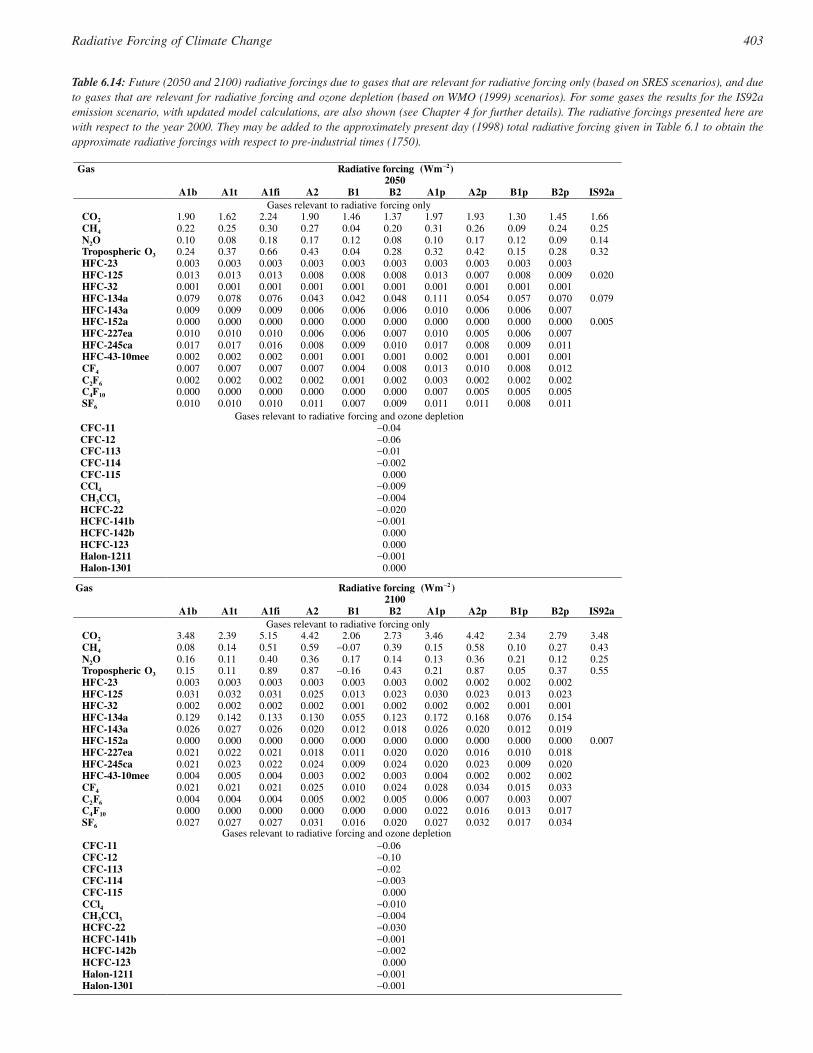
403Radiative Forcing of Climate Change
Table 6.14: Future (2050 and 2100) radiative forcings due to gases that are relevant for radiative forcing only (based on SRES scenarios), and dueto gases that are relevant for radiative forcing and ozone depletion (based on WMO (1999) scenarios). For some gases the results for the IS92aemission scenario, with updated model calculations, are also shown (see Chapter 4 for further details). The radiative forcings presented here arewith respect to the year 2000. They may be added to the approximately present day (1998) total radiative forcing given in Table 6.1 to obtain theapproximate radiative forcings with respect to pre-industrial times (1750).
Gas Radiative forcing (Wm−2)2050
A1b A1t A1fi A2 B1 B2 A1p A2p B1p B2p IS92aGases relevant to radiative forcing only
CO2 1.90 1.62 2.24 1.90 1.46 1.37 1.97 1.93 1.30 1.45 1.66CH4 0.22 0.25 0.30 0.27 0.04 0.20 0.31 0.26 0.09 0.24 0.25N2O 0.10 0.08 0.18 0.17 0.12 0.08 0.10 0.17 0.12 0.09 0.14Tropospheric O3 0.24 0.37 0.66 0.43 0.04 0.28 0.32 0.42 0.15 0.28 0.32HFC-23 0.003 0.003 0.003 0.003 0.003 0.003 0.003 0.003 0.003 0.003HFC-125 0.013 0.013 0.013 0.008 0.008 0.008 0.013 0.007 0.008 0.009 0.020HFC-32 0.001 0.001 0.001 0.001 0.001 0.001 0.001 0.001 0.001 0.001HFC-134a 0.079 0.078 0.076 0.043 0.042 0.048 0.111 0.054 0.057 0.070 0.079HFC-143a 0.009 0.009 0.009 0.006 0.006 0.006 0.010 0.006 0.006 0.007HFC-152a 0.000 0.000 0.000 0.000 0.000 0.000 0.000 0.000 0.000 0.000 0.005HFC-227ea 0.010 0.010 0.010 0.006 0.006 0.007 0.010 0.005 0.006 0.007HFC-245ca 0.017 0.017 0.016 0.008 0.009 0.010 0.017 0.008 0.009 0.011HFC-43-10mee 0.002 0.002 0.002 0.001 0.001 0.001 0.002 0.001 0.001 0.001CF4 0.007 0.007 0.007 0.007 0.004 0.008 0.013 0.010 0.008 0.012C2F6 0.002 0.002 0.002 0.002 0.001 0.002 0.003 0.002 0.002 0.002C4F10 0.000 0.000 0.000 0.000 0.000 0.000 0.007 0.005 0.005 0.005SF6 0.010 0.010 0.010 0.011 0.007 0.009 0.011 0.011 0.008 0.011
Gases relevant to radiative forcing and ozone depletionCFC-11 −0.04CFC-12 −0.06CFC-113 −0.01CFC-114 −0.002CFC-115 0.000CCl4 −0.009CH3CCl3 −0.004HCFC-22 −0.020HCFC-141b −0.001HCFC-142b 0.000HCFC-123 0.000Halon-1211 −0.001Halon-1301 0.000
Gas Radiative forcing (Wm−2 )2100
A1b A1t A1fi A2 B1 B2 A1p A2p B1p B2p IS92aGases relevant to radiative forcing only
CO2 3.48 2.39 5.15 4.42 2.06 2.73 3.46 4.42 2.34 2.79 3.48CH4 0.08 0.14 0.51 0.59 −0.07 0.39 0.15 0.58 0.10 0.27 0.43N2O 0.16 0.11 0.40 0.36 0.17 0.14 0.13 0.36 0.21 0.12 0.25Tropospheric O3 0.15 0.11 0.89 0.87 −0.16 0.43 0.21 0.87 0.05 0.37 0.55HFC-23 0.003 0.003 0.003 0.003 0.003 0.003 0.002 0.002 0.002 0.002HFC-125 0.031 0.032 0.031 0.025 0.013 0.023 0.030 0.023 0.013 0.023HFC-32 0.002 0.002 0.002 0.002 0.001 0.002 0.002 0.002 0.001 0.001HFC-134a 0.129 0.142 0.133 0.130 0.055 0.123 0.172 0.168 0.076 0.154HFC-143a 0.026 0.027 0.026 0.020 0.012 0.018 0.026 0.020 0.012 0.019HFC-152a 0.000 0.000 0.000 0.000 0.000 0.000 0.000 0.000 0.000 0.000 0.007HFC-227ea 0.021 0.022 0.021 0.018 0.011 0.020 0.020 0.016 0.010 0.018HFC-245ca 0.021 0.023 0.022 0.024 0.009 0.024 0.020 0.023 0.009 0.020HFC-43-10mee 0.004 0.005 0.004 0.003 0.002 0.003 0.004 0.002 0.002 0.002CF4 0.021 0.021 0.021 0.025 0.010 0.024 0.028 0.034 0.015 0.033C2F6 0.004 0.004 0.004 0.005 0.002 0.005 0.006 0.007 0.003 0.007C4F10 0.000 0.000 0.000 0.000 0.000 0.000 0.022 0.016 0.013 0.017SF6 0.027 0.027 0.027 0.031 0.016 0.020 0.027 0.032 0.017 0.034
Gases relevant to radiative forcing and ozone depletionCFC-11 −0.06CFC-12 −0.10CFC-113 −0.02CFC-114 −0.003CFC-115 0.000CCl4 −0.010CH3CCl3 −0.004HCFC-22 −0.030HCFC-141b −0.001HCFC-142b −0.002HCFC-123 0.000Halon-1211 −0.001Halon-1301 −0.001
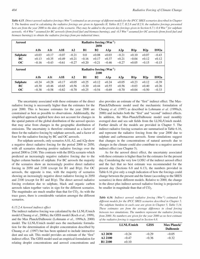
The uncertainty associated with these estimates of the directradiative forcing is necessarily higher than the estimates for theyear 2000. This is because estimates for the year 2000 areconstrained as best as possible to observations. Additionally, thesimplified approach applied here does not account for changes inthe spatial pattern of the global distribution of the aerosol speciesthat may arise from changes in the geographic distribution ofemissions. The uncertainty is therefore estimated as a factor ofthree for the radiative forcing by sulphate aerosols, and a factor offour for the radiative forcing by BC and OC aerosols.
For sulphate aerosols, only scenarios A1fi, A2, and A2p showa negative direct radiative forcing for the period 2000 to 2050,with all scenarios showing positive radiative forcings over theperiod 2000 to 2100. This contrasts with the IS92a scenario whichpredicted an increasingly negative radiative forcing due to thehigher column burden of sulphate. For BC aerosols the majorityof the scenarios show an increasingly positive direct radiativeforcing in 2050 and 2100 (except for B1 and B1p). For OCaerosols, the opposite is true, with the majority of scenariosshowing an increasingly negative direct radiative forcing in 2050and 2100 (except for B1 and B1p). The direct aerosol radiativeforcing evolution due to sulphate, black and organic carbonaerosols taken together varies in sign for the different scenarios.The magnitudes are much smaller than that for CO2. As with thetrace gases, there is considerable variation amongst the differentscenarios.
6.15.2.4 Aerosol indirect effectThe indirect radiative forcing was calculated by the LLNL/Umichmodel (Chuang et al., 2000a), the GISS model (Koch et al., 1999),and the Max Planck/Dalhousie (Lohmann et al., 1999a,b, 2000)model. The LLNL/Umich model uses the mechanistic formula-tion for the determination of droplet concentration described byChuang et al. (1997) but has been updated to include interactivedust and sea salt. This model provides an estimate of the “first”indirect effect. The GISS model used an empirical formulation forrelating droplet concentrations and aerosol concentrations and
also provides an estimate of the “first” indirect effect. The Max-Planck/Dalhousie model used the mechanistic formulation ofChuang et al. (1997) as described in Lohmann et al. (1999a,b,2000) and includes both the “first” and “second” indirect effects.In addition, the Max-Planck/Dalhousie model used monthlyaveraged dust and sea salt fields from the LLNL/Umich model.Further details of the models are provided in Chapter 5. Theindirect radiative forcing scenarios are summarised in Table 6.16,and represent the radiative forcing from the year 2000 due tosulphate and carbonaceous aerosols. Some simulations suggestthat changes in the concentrations of natural aerosols due tochanges in the climate could also contribute to a negative aerosolindirect effect (see Chapter 5).
As for the aerosol direct effect, the uncertainty associatedwith these estimates is higher than for the estimates for the presentday. Considering the very low LOSU of the indirect aerosol effectand the fact that no best estimate was recommended for thepresent day (Sections 6.8 and 6.13), the numbers provided inTable 6.16 give only a rough indication of how the forcings couldchange between the present and the future (according to the SRESscenarios) in three different models. Relative to 2000, the changein the direct plus indirect aerosol radiative forcing is projected tobe smaller in magnitude than that of CO2.
404 Radiative Forcing of Climate Change
Table 6.15. Direct aerosol radiative forcings (Wm−2) estimated as an average of different models for the IPCC SRES scenarios described in Chapter5. The burdens used in calculating the radiative forcings are given in Appendix II, Tables II.2.7, II.2.8 and II.2.9, the radiative forcings presentedhere are from the year 2000 to the date of the scenario. They may be added to the present day forcings given in Section 6.7 (−0.4 Wm−2 for sulphateaerosols, +0.4 Wm−2 assumed for BC aerosols (from fossil fuel and biomass burning), and –0.5 Wm−2 assumed for OC aerosols (from fossil fuel andbiomass burning)) to obtain the radiative forcings from pre-industrial times.
Table 6.16: Indirect aerosol radiative forcing (Wm−2) estimated bydifferent models for the IPCC SRES scenarios described in Chapter 5.The sulphate burdens in each case are given in Chapter 5, Table 5.14.These estimates are from the average difference in cloud forcingbetween two simulations. The numbers represent the radiative forcingfrom 2000. No numbers are given for the year 2000 as no best estimateof the radiative forcing is suggested in Section 6.8.
Aerosol Radiative forcing (Wm−2 )2050
A1b A1t A1fi A2 B1 B2 A1p A2p B1p B2p IS92a
Sulphate +0.03 +0.17 −0.07 −0.21 0.0 +0.08 +0.03 −0.21 +0.10 +0.07 −0.43BC +0.13 +0.35 +0.49 +0.21 −0.16 +0.17 +0.37 +0.21 −0.04 +0.12 +0.12OC −0.16 −0.43 −0.61 −0.27 +0.20 −0.21 −0.46 −0.27 +0.05 −0.15 −0.15
Aerosol Radiative forcing (Wm−2 )2100
A1b A1t A1fi A2 B1 B2 A1p A2p B1p B2p IS92a
Sulphate +0.24 +0.28 +0.17 +0.05 +0.25 +0.12 +0.24 +0.05 +0.23 +0.12 −0.39BC +0.30 +0.46 +0.65 +0.56 −0.20 +0.44 +0.55 +0.56 −0.03 +0.40 +0.26OC −0.38 −0.58 −0.82 −0.70 +0.25 −0.54 −0.69 −0.70 +0.04 −0.50 −0.33
LLNL/Umich GISS Max Planck/Dalhousie
A2 2030 −0.24 −0.29 −0.05A2 2100 −0.47 −0.36 −0.32B1 2100 +0.10
Appendix 6.1 Elements of Radiative Forcing Concept
The principal elements of the radiative forcing concept aresummarised below.
(A) The concept was developed first in the context of the one-dimensional radiative-convective models that investigated theequilibrated global, annual mean surface temperature responsesto radiative perturbations caused by changes in the concentrationsof radiatively active species (Manabe and Wetherald, 1967;Ramanathan and Coakley, 1978; WMO, 1986). Over the pastdecade, the concept has been extended to cover different spatialdimensions and seasonal time-scales (IPCC, 1992, 1994).
(B) In the one-dimensional radiative-convective modelframework, the surface and troposphere are closely coupled,behaving as a single thermodynamic system under the jointcontrol of radiative and convective processes, with a specifiedlapse rate determining the thermal structure. The stratosphericstate is determined by the radiative equilibrium condition. Thestratosphere and troposphere irradiances are together constrainedby the requirement that the top of the atmosphere net total irradi-ance (i.e., radiative energy absorbed minus that emitted by theEarth’s entire climate system) must be zero at equilibrium. Inapplying the forcing concept to arbitrary spatial and seasonaltime-scales, as opposed to the global annual mean, it has beenassumed (WMO, 1992; SAR) that the stratosphere is in radiative-dynamical (rather than radiative) equilibrium (see (D) below).
(C) The stratosphere is a fast response system which, in responseto an imposed radiative perturbation, comes into equilibrium ona time-scale (about a few months) that is much more rapid thanthe surface-troposphere system (typically decades) (Hansen etal., 1997a; Shine and Forster, 1999). The latter is a slow responsesystem owing principally to the thermal inertia of the oceans.
(D) When a perturbation is applied (such as increases in well-mixed greenhouse gases), there is an instantaneous change inirradiances that is manifest in general as a radiative imbalance(forcing) at the surface, tropopause and the top of the atmosphere.The rapid thermal re-equilibration of the stratosphere leads to analteration of the radiative imbalance imposed on the surface-troposphere system (WMO, 1992), thereby yielding an adjustedforcing (SAR). The surface and troposphere, operating in a slowresponse mode, are still in a process of adjustment while thestratosphere has already reached its new equilibrium state. TheSAR points out the clear distinction existing between the instan-taneous and adjusted forcings.
For the arbitrary space and time mean stratosphere, there arisesthe need to evaluate the radiative flux changes with the strato-sphere in a radiative-dynamical equilibrium. A classical methodto determine this is the “Fixed Dynamical Heating” (FDH;WMO, 1995) in which it is assumed that the dynamical heatingrate in the stratosphere is unchanged and that the stratospherecomes to a new thermal equilibrium in response to the perturba-tion through adjustments in the temperature profile, such that a
new radiative-dynamical equilibrium is attained (radiativeresponse; see Ramanathan and Dickinson (1979) and Fels et al.(1980)). The resulting adjustment process in the stratospheremakes an additional contribution to the forcing of the surface-troposphere system. When the stratosphere has adjusted to a newradiative-dynamical equilibrium with resultant changes to itsthermal state, the change in flux at the tropopause and at the topof the atmosphere become identical. It is important that thestratosphere be in radiative-dynamical equilibrium and, as shownby Hansen et al. (1997a), it is the adjusted rather than the instan-taneous forcing that is a more relevant indicator of the surfacetemperature response. The adjustment of stratosphere is crucialfor some of the forcings, but not for all of them (Shine andForster, 1999). In the case of some radiative perturbations, thestratosphere is hardly perturbed and the instantaneous andadjusted radiative flux changes thus tend to be similar (SAR). Inother cases, there is only a small (20% or less) influence due tothe stratospheric adjustment process. However, for the case ofozone depletion in the lower stratosphere, the effect of a strato-spheric adjustment could even yield a change in the sign of theforcing.
(E) As a direct consequence of the above, the forcing definitionmost appropriate for the response of the surface-tropospheresystem to a radiative perturbation is the net (down minus up)radiative (solar plus long-wave) change defined at the tropopauseafter the stratosphere has come to a new thermal equilibriumstate. Thus, the level at which the tropopause is assumed in themodels is an important aspect for the quantitative determinationof the forcing (Forster et al., 1997), as is the model verticalresolution used to resolve the vicinity of the tropopause region(Shine et al., 1995). The classical radiative-convective modeldefinition of the tropopause considers it as a boundary between aregion where radiative-convective equilibrium prevails (i.e.,troposphere) and a region that is in radiative (or radiative-dynamical, i.e., stratosphere) equilibrium. Such a distinctioncould be ambiguous in the case of the three-dimensional GCMsor the real world. However, radiative forcing appears to berelatively robust to changes in the definition of the tropopause ina GCM (Christiansen, 1999).
(F) A major motivation for the radiative forcing concept is theease of climate change analysis when radiative forcing, feedback,and climate response are distinguished from one another. Such aseparation is possible in the modelling framework where forcingand feedback can be evaluated separately e.g., for the case of CO2
doubling effects (see Dickinson, 1982; Dickinson and Cicerone,1986; Cess and Potter, 1988; Cess et al., 1993). The considera-tion of forcing, feedback and response as three distinct entities inthe modelling framework (see also Charlson, 2000) whileoriginating from the one-dimensional radiative/convectivemodels, has made the transition to GCM studies of climate(Hansen et al., 1981; Wetherald and Manabe, 1988; Chen andRamaswamy, 1996a).
(G) A critical aspect of the separability mentioned in (F) isholding the surface and troposphere state fixed in the evaluation
405Radiative Forcing of Climate Change
of the radiative forcing. For example, in the case of a change inthe concentration of a radiatively active species, the term “state”implies that all parameters are held at the unperturbed values withonly the concerned species’ concentration being changed. Thus,in the strictest sense, temperature in the troposphere, watervapour and clouds in the entire atmosphere, and circulation, areheld fixed in the computation of the irradiance changes at thetropopause, with only the stratosphere adjusted to a new thermalequilibrium state via the radiative response. In contrast to thisprescription for calculating the forcing, the resulting changes inthe meteorological and climatic parameters (e.g., tropospherictemperature and water vapour) constitute responses to theimposed perturbation (WMO, 1986; Charlson, 2000). In theIPCC context, the change in a radiative agent’s characteristic hasinvolved anthropogenic (e.g., CO2) and natural (e.g., aerosolsafter a volcanic eruption) perturbations.
It is important to emphasise that changes in water vapour in thetroposphere are viewed as a feedback variable rather than aforcing agent. However, in the case of the second indirect aerosolforcing, the separation is less distinct. Anthropogenic emissions(e.g., aircraft, fossil fuel) or precursors to water vapour arenegligible. The same is true for changes in water vapour in thestratosphere, except in the instance that the oxidation of CH4
provides an input. Changes in the condensed liquid and solidphases of water (i.e., clouds) are also considered as part of theclimate feedback. The strict requirement of no feedbacks in thesurface and troposphere demands that no secondary effects suchas changes in troposphere motions or its thermodynamic state, ordynamically-induced changes in water substance in the surfaceand atmosphere, be included in the evaluation of the net irradi-ance change at the tropopause. (Note: the second indirect effectof aerosols consists of microphysically-induced changes in thewater substance.)
(H) The foregoing governing factors reflect the fundamentalrecognition that, in response to an externally imposed radiativeforcing, there is a shift in the equilibrium state of the climatesystem. This forcing of the climate change in the IPCC parlanceis to be distinguished from forcing definitions initiated for otherpurposes, e.g., cloud forcing (Ramanathan et al., 1989), seasurface temperature related forcing during ENSO periods, etc.
References
Abbas, M.A. and J. Latham, 1969: The electrofreezing of supercooledwater drops. J. Met. Soc. Japan, 47, 65-74.
Ackerman, S.A. and H. Chung, 1992: Radiative effects of airborne duston regional energy budgets at the top of the atmosphere. J. Appl.Meteor., 31, 223-233.
Ackerman, A.S., O.B. Toon, D.E. Stevens, A.J. Heymsfield, V.Ramanathan, and E.J. Welton, 2000: Reduction of tropical cloudinessby soot. Science, 288, 1042-1047.
Adams, P.J., J.H. Seinfeld, D.M. Koch, L Mickley, and D. Jacob, 2001:General circulation model assessment of direct radiative forcing bythe sulfate-nitrate-ammonium-water inorganic aerosol system. J.Geophys. Res., 106, 1097-1111.
Albrecht, B.A., 1989: Aerosols, cloud microphysics, and fractionalcloudiness. Science, 245, 1227-1230.
Allen, D., K. Pickering, G. Stenchikov, A. Thompson, and Y. Kondo,2000: A three-dimensional total odd nitrogen (NOy) simulationduring SONEX using a stretched-grid chemical transport model. J.Geophys. Res., 105, 3851-3876.
Andronova, N.G., E.V. Rozanov, F. Yang. M.E. Schlesinger, and G.L.Stenchikov, 1999: Radiative forcing by volcanic aerosols from 1850through 1994. J. Geophys. Res., 104, 16807-16826.
Arnold, N.F. and T.R. Robinson, 1998: Solar cycle changes to planetarywave propagation and their influence on the middle atmospherecirculation. Annal. Geophys., 16, 69-76.
Baliunas, S. and R. Jastrow, 1990: Evidence for long-term brightnesschanges of solar-type stars. Nature, 348, 520-523.
Ballard, J., R.J. Knight, D.A. Newnham, J. Vander Auwera, M. Herman,G. Di Lonardo, G. Masciarelli, F.M. Nicolaisen, J.A. Beukes, L.K.Christensen, R. McPheat, G. Duxbury, R. Freckleton, and K.P. Shine,2000: An intercomparison of laboratory measurements of absorptioncross-sections and integrated absorption intensities for HCFC-22. J.Quant. Spectrosc. Radiat. Transfer., 66, 109-128.
Barry, J., G. Locke, D. Scollard, H. Sidebottom, J. Treacy, C. Clerbaux,R. Colin, and J. Franklin, 1997: 1,1,1,3,3,-pentafluorobutane (HFC-365mfc): Atmospheric degradation and contribution to radiativeforcing. Int. J. Chem. Kinet., 29, 607-617.
Beer, J., S.T. Baumgartner, B. Dittrich-Hannen, J. Hauenstein, P. Kubik,C. Lukasczyk, W. Mende, R. Stellmacher, and M. Suter, 1994: Solarvariability traced by cosmogenic isotopes. In: The Sun as a VariableStar [Pap, J.M., C. Fröhlich, H.S. Hudson, and S.K. Solanki (eds.)].CUP 291-300.
Bekki, S., K.S. Law, and J.A. Pyle, 1994: Effect of ozone depletion onatmospheric CH4 and CO concentrations. Nature, 371, 595-597.
Berger, A., C. Tricot, H. Gallée, and M.F. Loutre, 1993: Water vapor,CO2 and insolation over the last glacial-interglacial cycles. Phil.Trans. Roy. Soc. London. B, 341, 253-261.
Berntsen, T.K. and I.S.A. Isaksen, 1999: Effects of lightning and convec-tion on changes in tropospheric ozone due to NOx emissions fromaircraft. Tellus, 51B, 766-788.
Berntsen, T., I.S.A. Isaksen, W.-C. Wang, and X-Z. Liang, 1996: Impactsof increased anthropogenic emissions in Asia on tropospheric ozoneand climate. Tellus, 48B, 13-32.
Berntsen, T.K., I.S.A. Isaksen, G. Myhre, J.S. Fuglestvedt, F. Stordal, T.A. Larsen, R.S. Freckleton, and K.P. Shine, 1997: Effects of anthro-pogenic emissions on tropospheric ozone and its radiative forcing. J.Geophys. Res., 102, 28101-28126.
Berntsen, T.K., G. Myhre, F. Stordal, and I.S.A. Isaksen, 2000: Timeevolution of tropospheric ozone and its radiative forcing. J. Geophys.Res., 105, 8915-8930.
Betts, R., 2001: Biogeophysical impacts of land use on present-dayclimate: near-surface temperature and radiative forcing. Atmos. Sci.Lett., doi:10.1006/asle.2000.0023.
Bintanja, R., J.P.F. Fortuin, and H. Kelder, 1997: Simulation of the
406 Radiative Forcing of Climate Change
meridionally and seasonally varying climate response caused bychanges in ozone concentration. J. Climate, 10, 1288-1311.
Boucher, O., 1995: GCM estimate of the indirect aerosol forcing usingsatellite-retrieved cloud effective droplet radii. J. Climate, 8, 1403-1409.
Boucher, O., 1999: Aircraft can increase cirrus cloudiness. Nature, 397,30-31.
Boucher, O. and H. Rodhe, 1994: The sulfate-CCN-cloud albedo effect:A sensitivity study. Report CM-83, Department of Meteorology,Stockholm University, 20 pp.
Boucher, O. and T.L. Anderson, 1995: GCM assessment of thesensitivity of direct climate forcing by anthropogenic sulfate aerosolsto aerosol size and chemistry. J. Geophys. Res., 100, 26117-26134.
Boucher, O. and U. Lohmann, 1995: The sulfate-CCN-cloud albedoeffect: A sensitivity study using two general circulation models.Tellus, 47B, 281-300.
Boucher, O. and D. Tanré, 2000: Estimation of the aerosol perturbationto the Earth’s radiative budget over oceans using POLDER satelliteaerosol retrievals. Geophys. Res. Lett., 27, 1103-1106.
Boucher, O., H. Le Treut, and M.B. Baker, 1995: Precipitation andradiation modelling in a GCM: Introduction of cloud microphysics.J. Geophys. Res., 100, 16395-16414.
Boucher, O., S.E. Schwartz, T.P. Ackerman, T.L. Anderson, B.Bergstrom, B. Bonnel, P. Chylek, A. Dahlback, Y. Fouquart, Q. Fu,R.N. Halthore, J.M. Haywood, T. Iversen, S. Kato, S. Kinne, A.Kirkevåg, K.R. Knapp, A. Lacis, I. Laszlo, M.I. Mishchenko, S.Nemesure, V. Ramaswamy, D.L. Roberts, P. Russell, M.E.Schlesinger, G.L. Stephens, R. Wagener, M. Wang, J. Wong, and F.Yang, 1998: Intercomparison of models representing directshortwave radiative forcing by sulfate aerosols. J. Geophys. Res., 103,16979-16998.
Brasseur, G.P., J.T. Kiehl, J.-F. Muller, T. Schneider, C. Granier, X.X.Tie, and D. Hauglustaine, 1998: Past and future changes in globaltropospheric ozone: impact on radiative forcing. Geophys. Res. Lett.,25, 3807-3810.
Brueckner, G.E., K.L. Edlow, L.E. Floyd, J.L. Lean, and M.E.VanHoosier, 1993: The Solar Ultraviolet Spectral Irradiance Monitor(SUSIM) experiment on board the Upper Atmosphere ResearchSatellite (UARS). J. Geophys. Res., 98, 10695-10711.
Brühl, C., 1993: The impact of the future scenarios for methane and otherchemically active gases on the GWP of methane. Chemosphere, 26,731-738.
Capaldo, K., J.J. Corbett, P. Kasibhatla, P. Fischbeck, and S.N. Pandis,1999: Effects of ship emissions on sulphur cycling and radiativeclimate forcing over the ocean. Nature, 400, 743-746.
Cavalli, F., M. Glasius, S. Hjorth, B. Rindone, and N. R. Jensen, 1998:Atmospheric lifetimes, infrared spectra, and degradation products ofa series of hydrofluoroethers. Atmos. Env., 32, 3767-3773.
Cebula, R. P., M.T. DeLand, and E. Hilsenrath, 1998: NOAA 11 SolarBackscattered Ultraviolet, model 2 (SBUV/2) instrument solarspectral irradiance measurements in 1989-1994. 1. Observations andlong-term calibration. J. Geophys. Res., 103, 16235-16249.
Cess, R.D. and G.L. Potter, 1988: A methodology for understanding andintercomparing atmospheric climate feedback processes in GCMs. J.Geophys. Res., 93, 8305-8314.
Cess, R.D., M.-H. Zhang, G.L. Potter, H.W. Barker, R.A. Colman, D.A.Dazlich, A.D. Del Genio, M. Esch, J.R. Fraser, V. Galin, W.L. Gates,J.J. Hack, W.J. Ingram, J.T. Kiehl, A.A. Lacis, H. Le Treut, Z.-X. Li,X.Z. Liang, J.-F. Mahfouf, B.J. McAvaney, K.P. Meleshko, J.-J.Morcrette, D.A. Randall, E. Roeckner, J.-F. Royer, A.P. Sokolov, P.V.Sporyshev, K.E. Taylor, W.-C. Wang, and R.T. Wetherald, 1993:Uncertainties in CO2 radiative forcing in atmospheric general circula-tion models. Science, 262, 1252-1255.
Chalita, S., D.A. Hauglustaine, H. Le Treut, and J.-F. Müller, 1996:Radiative forcing due to increased tropospheric ozone concentra-
tions. Atmos. Env., 30, 1641-1646.Chandra, S., J.R. Ziemke, W. Min, and W.G. Read, 1998: Effects of
1997-1998 El Niño on tropospheric ozone and water vapor. Geophys.Res. Lett., 25, 3867-3870.
Chandra, S., J.R. Ziemke, and R.W. Stewart, 1999: An 11-year solarcycle in tropospheric ozone from TOMS measurements. Geophys.Res. Lett., 26, 185-188.
Charlson, R.J., 2000: The coupling of biogeochemical cycles andclimate: Forcings, feedbacks and responses. In “Earth SystemSciences: from Biogeochemical Cycles to Global Change”,Academic Press.
Charlson, R.J., S.E. Schwartz, J.M. Hales, R.D. Cess, J.A. Coakley, J.E.Hansen, and D.J. Hofmann, 1992: Climate forcing by anthropogenicaerosols. Science, 255, 423-430.
Charlson, R.J., T.L. Anderson, and H. Rodhe, 1999: Direct climateforcing by anthropogenic aerosols: quantifying the link betweensulfate and radiation. Contrib. Atmos. Phys., 72, 79-94.
Chazette, P., C. Clerbaux, and G. Mégie, 1998: Direct estimate ofmethane radiative forcing by use of nadir spectral radiances. AppliedOptics, 37, 3113-3120.
Chen, C-T. and V. Ramaswamy, 1996a: Sensitivity of simulated globalclimate to perturbations in low cloud microphysical properties. I.Globally uniform perturbations. J. Climate, 9, 1385-1402.
Chen, C-T. and V. Ramaswamy, 1996b: Sensitivity of simulated globalclimate to perturbations in low cloud microphysical properties. II.Spatially localized perturbations. J. Climate, 9, 2788-2801.
Chin, M. and D.J. Jacob, 1996: Anthropogenic and natural contributionsto tropospheric sulfate: a global model analysis. J. Geophys. Res.,101, 18691-18699.
Christiansen, B., 1999: Radiative forcing and climate sensitivity: Theozone experience. Quart. J. R. Meteorol. Soc., 125, 3011-3035.
Christensen, L.K., J. Sehested, O.J. Nielsen, M. Bilde, T.J. Wallington,A. Guschin, L.T. Molina, and M.J. Molina, 1998: Atmosphericchemistry of HFE-7200 (C4F9OC2H5): Reaction with OH radicals,fate of C4F9OCH2CH2O and C4F9OCHO CH3 radicals. J. Phys.Chem. A, 102, 4839-4845.
Christidis, N., M.D. Hurley, S. Pinnock, K.P. Shine, and T.J. Wallington,1997: Radiative forcing of climate change by CFC-11 and possibleCFC replacements. J. Geophys. Res., 102, 19597-19609.
Christopher, S.A., D.V., Kliche, J. Chou, and R.M. Welch, 1996: Firstestimates of the radiative forcing of aerosols generated from biomassburning using satellite data. J. Geophys. Res., 101, 21265-21273.
Chuang, C.C., J.E. Penner, K.E. Taylor, and J.J. Walton, 1994: Climateeffects of anthropogenic sulfate: Simulations from a coupledchemistry/climate model. In: Preprints of the Conference onAtmospheric Chemistry, Nashville, Tennessee, January 1994.American Meteorological Society, Boston, USA, pp. 170-174.
Chuang, C.C., J.E. Penner, K.E. Taylor, A.S. Grossman, and J.J. Walton,1997: An assessment of the radiative effects of anthropogenic sulfate.J. Geophys. Res., 102, 3761-3778.
Chuang, C.C., J.E. Penner, and Y. Zhang, 2000a: Simulations of aerosolindirect effect for IPCC emissions scenarios. In: Proceedings of the11th Symposium on Global Change Studies, January 9-14, 2000,Long Beach, California. American Meteorological Society, Boston,USA, pp. 320-323.
Chuang, C.C., J.E. Penner, J.M. Prospero, K.E. Grant and G.H. Rau,2000b: Effects of anthropogenic aerosols on cloud susceptibility: asensitivity study of radiative forcing to aerosol characteristics andglobal concentration. Lawrence Livermore National LaboratoryInternal Report, No. UCRL-JC-139097 Rev. 1., Lawrence LivermoreNational Laboratory, CA, USA.
Chylek, P. and J. Wong, 1995: Effect of absorbing aerosols on the globalradiation budget. Geophys. Res. Lett., 22, 929-931.
Chylek, P., G. Videen, and D. Ngo, 1995: Effect of black carbon on theoptical properties and climate forcing of sulfate aerosols. J. Geophys.
407Radiative Forcing of Climate Change
Res., 100, 16325-16332. Chylek, P., C.M. Banic, B. Johnson, P.A. Damiano, G.A. Isaac, W.R.
Leaitch, P.S.K. Liu, F.S. Boudala, B. Winter, and D. Ngo, 1996a:Black carbon: Atmospheric concentrations and cloud water contentmeasurements over southern Nova Scotia. J. Geophys. Res., 101,29105-29110.
Chylek, P., G.B. Lesins, G. Videen, J.G.D. Wong, R.G. Pinnick, D. Ngo,and J.D. Klett, 1996b: Black carbon and absorption of solar radiationby clouds. J. Geophys. Res., 101, 23365-23371.
Claquin, T., M. Schulz, Y. Balkanski, and O. Boucher, 1998:Uncertainties in assessing radiative forcing by mineral dust. Tellus,50B, 491-505.
Cooke, W.F. and J.J.N. Wilson, 1996: A global black carbon model. J.Geophys. Res., 101, 19395-19409.
Cooke, W.F., C. Liousse, H. Cachier, and J. Feichter, 1999: Constructionof a 1°x1° fossil-fuel emission dataset for carbonaceous aerosol andimplementation and radiative impact in the ECHAM-4 model. J.Geophys. Res., 104, 22137-22162.
Cox, S.J., W.-C. Wang, and S.E. Schwartz, 1995: Climate response toforcings by sulfate aerosols and greenhouse gases. Geophys. Res.Lett., 18, 2509-2512.
Crommelynk, D., A. Fichot, R.B. Lee III, and J. Romero, 1995: Firstrealisation of the space absolute radiometric reference (SARR)during the ATLAS 2 flight period. Adv. Spac. Res., 16, 17-23.
Daniel, J.S. and S. Solomon, 1998. On the climate forcing of carbonmonoxide. J. Geophys. Res., 103, 13249-13260.
Daniel, J.S., S. Solomon, and D. Albritton, 1995: On the evaluation ofhalocarbon radiative forcing and global warming potentials. J.Geophys. Res., 100, 1271-1285.
DeLand, M.T. and R.P. Cebula, 1998: NOAA 11 Solar BackscatteredUltraviolet, model 2 (SBUV/2) instrument solar spectral irradiancemeasurements in 1989-1994. 2. Results, validation, and comparisons.J. Geophys. Res., 103, 16251-16273.
Delobbe, L. and H. Gallée, 1998: Simulation of marine stratocumulus:Effect of precipitation parameterization and sensitivity to dropletnumber concentration. Boundary-Layer Meteorol., 89, 75-107.
DeMore, W.B., S.P. Sander, D.M. Golden, R.F. Hampson, M.J. Kurylo,C.J. Howard, A.R. Ravishankara, C.E. Kolb, and M.J. Molina, 1997:Chemical kinetics and photochemical data for use in stratosphericmodeling, Evaluation Number 12, JPL Publ. 97-4, Jet PropulsionLaboratory, Pasadena, Calif.
Dentener, F.J., G.R. Carmichael, Y. Zhang, J. Lelieveld, and P. Crutzen,1996: Role of mineral aerosol as a reactive surface in the globaltroposphere. J. Geophys. Res., 101, 22869-22889.
Dickinson, R.E., 1982: In: Carbon Dioxide Review [Clark, W.C. (ed.)].Clarendon, New York, NY, USA, pp. 101-133.
Dickinson, R.E., and R.J. Cicerone, 1986: Future global warming fromatmospheric trace gases. Nature, 319, 109-115.
van Dorland, R., F.J. Dentener, and J. Lelieveld, 1997: Radiative forcingdue to tropospheric ozone and sulfate aerosols. J. Geophys. Res., 102,28079-28100.
Emmons, L.K., M.A. Carroll, D.A. Hauglustaine, G.P. Brasseur, C.Atherton, J. Penner, S. Sillman, H. Levy, F. Rohrer, W.M.F. Wauben,P.F.J. Van Velthoven, Y. Wang, D. Jacob, P. Bakwin, R. Dickerson, B.Doddridge, C. Gerbig, R. Honrath, G. Hübler, D. Jaffe, Y. Kondo,J.W. Munger, A. Torres, and A. Volz-Thomas, 1997: Climatologies ofNOx and NOy: a comparison of data and models. Atmos. Env., 31,1851-1904.
Evans, W.F.J. and E. Puckrin, 1995: An observation of the greenhouseradiation associated with carbon monoxide. Geophys. Res. Lett., 22,925-928.
Evans, W.F.J. and E. Puckrin, 1999: A comparison of GCM models withexperimental measurements of surface radiative forcing bygreenhouse gases. 10th Symposium on Global Change Studies,American Meteorological Society, pp. 378-381, 10-15 January 1999,
Dallas, Texas.Evans, S.J., R. Toumi, J.E. Harries, M.P. Chipperfield, and J.M. Russell
III, 1998: Trends in stratospheric humidities and the sensitivity ofozone to these trends. J. Geophys. Res., 103, 8715-8725.
Fahey, D.W., U. Schumann, S. Ackerman, P. Artaxo, O. Boucher, M.Y.Danilin, B. Kärcher, P. Minnis, T. Nakajima, and O.B. Toon, 1999:Aviation-produced aerosols and cloudiness. In: IntergovernmentalPanel on Climate Change Special Report on Aviation and the GlobalAtmosphere [Penner, J.E., D.H. Lister, D.J. Griggs, D.J. Dokken, andM. McFarland (eds.)]. Cambridge University Press, Cambridge,United Kingdom and New York, NY, USA, pp. 65-120.
Farrar, P.D., 2000: Are cosmic rays influencing oceanic cloud coverage– Or is it only El Niño? Clim. Change, 47, 7-15.
Feichter, J., U. Lohmann, and I. Schult, 1997: The atmospheric sulfurcycle in ECHAM-4 and its impact on the shortwave radiation. Clim.Dyn., 13, 235-246.
Fels, S.B., J.D. Mahlman, M.D. Schwarzkopf, and R.W. Sinclair, 1980:Stratospheric sensitivity to perturbations in ozone and carbondioxide: Radiative and dynamical response. J. Atmos. Sci., 37, 2265-2297.
Fishman, J., 1991: The global consequences of increasing troposphericozone concentrations. Chemosphere, 22, 685-695.
Fishman, J. and V.G. Brackett, 1997: The climatological distribution oftropospheric ozone derived from satellite measurements usingversion 7 Total Ozone Mapping Spectrometer and StratosphericAerosol and Gas Experiment data sets. J. Geophys. Res., 102, 19275-19278.
Fleming, E.L., S. Chandra, C.H. Jackman, D.B. Considine, and A.R.Douglass, 1995: The middle atmosphere response to short and longterm UV variations: An analysis of observations and 2D modelresults. J. Atmos. Terr. Phys., 57, 333-365.
Floyd, L.E., P.A. Reiser, P.C. Crane, L.C. Herring, D.K. Prinz, and G.E.Brueckner, 1998: Solar cycle 22 UV spectral irradiance variability:Current measurements by SUSIM UARS. Solar Phys., 177, 79-87.
Forster, P.M. de F., 1999: Radiative forcing due to stratospheric ozonechanges 1979-1997, using updated trend estimates, J. Geophys. Res.,104, 24,395-24,399.
Forster, P. M. de F. and K.P. Shine, 1999: Stratospheric water vapourchanges as a possible contributor to observed stratospheric cooling,Geophys. Res. Lett., 26, 3309-3312.
Forster, P.M. de F. and K.P. Shine, 1997: Radiative forcing and temper-ature trends from stratospheric ozone changes. J. Geophys. Res., 102,10841-10857.
Forster, P.M. de F., R.S. Freckleton, and K.P. Shine, 1997: On aspects ofthe concept of radiative forcing. Clim. Dyn., 13, 547-560.
Forster, P.M. de F., M. Blackburn, R. Glover, and K.P. Shine, 2001: Anexamination of climate sensitivity for idealized climate changeexperiments in an intermediate general circulation model. Clim.Dyn., 16, 833-849.
Fortuin, J.P.F. and H. Kelder, 1996: Possible links between ozone andtemperature profiles. Geophys. Res. Lett., 23, 1517-1520.
Fowler, L.D., D.A. Randall, and S.A. Rutledge, 1996: Liquid and icecloud microphysics in the CSU general circulation model. Part I:Model description and simulated microphysical processes. J.Climate, 9, 489-529.
Freckleton, R.S., S. Pinnock, and K.P. Shine, 1996: Radiative forcing ofhalocarbons: A comparison of line-by-line and narrow-band modelsusing CF4 as an example. J. Quant. Spectrosc. Radiat. Transfer, 55,763-769.
Freckleton, R.S., E.J. Highwood, K.P. Shine, O. Wild, K.S. Law, andM.G. Sanderson, 1998: Greenhouse gas radiative forcing: Effects ofaveraging and inhomogeneities in trace gas distribution. Q. J. R.Meteorol. Soc., 124, 2099-2127.
Fröhlich, C. and J. Lean, 1998: The Sun’s total irradiance: Cycles, trendsand related climate change uncertainties since 1976. Geophys. Res.
408 Radiative Forcing of Climate Change
Lett., 25, 4377-4380.Fuglestvedt, J.S., J.E. Jonson, and I.S.A. Isaksen, 1994: Effects of
reduction in stratospheric ozone on tropospheric chemistry throughchanges in photolysis rates. Tellus, 46B, 172-192.
Fuglestvedt, J.S., J.E. Jonson, W.-C. Wang, and I.S.A. Isaksen, 1995:Response in tropospheric chemistry to changes in UV fluxes, temper-atures and water vapor densities. In: Atmospheric Ozone as a ClimateGas [Wang, W.-C. and I.S.A. Isaksen (eds.)]. NATO Series I 32,Springer-Verlag, Berlin, Germany, pp. 143-162.
Fuglestvedt, J.S., I.S.A. Isaksen, and W.-C. Wang, 1996: Estimates ofindirect global warming potentials for CH4, CO, and NOx. Clim.Change, 34, 405-437.
Fuglestvedt, J.S., T.K. Berntsen, I.S.A. Isaksen, H. Mao, X.-Z. Liang,and W.-C. Wang, 1999: Climate forcing of nitrogen oxides throughchanges in tropospheric ozone and methane: global 3D modelstudies. Atmos. Env., 33, 961-977.
Fuglestvedt, J. S., T. K. Berntsen, O. Godal, and T. Skodvin, 2000:Climate implications of GWP-based reductions in greenhouse gasemissions. Geophys. Res. Lett., 27, 409-412.
Ghan, S. and R. Easter, 1998: Comments: A limited-area-model casestudy of the effects of sub-grid scale variations in relative humidityand cloud upon the direct radiative forcing of sulfate aerosol.Geophys. Res. Lett., 25, 1039-1040.
Ghan, S.J., G. Guzman, and H. Abdul-Razzak, 1998: Competitionbetween sea salt and sulfate particles as cloud condensation nuclei. J.Atmos. Sci., 55, 3340-3347.
Ghan, S.J., R.C. Easter, E. Chapman, H. Abdul-Razzak, Y. Zhang, R.Leung, N. Laulainen, R. Saylor, and R. Zaveri, 2001a: A physically-based estimate of radiative forcing by anthropogenic sulfate aerosol.J. Geophys. Res., in press.
Ghan, S., R. Easter, J. Hudson, and F.-M. Bréon, 2001b: Evaluation ofaerosol indirect radiative forcing in MIRAGE. J. Geophys. Res., inpress.
Gierczak, T., R.K. Talukdar, J.B. Burdkholder, R.W. Portmann, J.S.Daniel, S. Solomon, and A.R. Ravishankara, 1996: Atmospheric fateand greenhouse warming potentials of HFC-236fa and HFC-236ea.J. Geophys. Res., 101, 12905-12911.
Gierens, K. and M. Ponater, 1999: Comment on “Variation of cosmic rayflux and global cloud coverage - a missing link in solar-climaterelationships” by H. Svensmark and E. Friis-Christensen. J. Atmos.Solar-Terrest. Phys., 61, 795-797.
Good, D.A., J.S. Francisco, A.K. Jain, D.J. Wuebbles, 1998: Lifetimesand global warming potentials for dimethyl ether and for fluorinatedethers: CH3OCF3 (E143a), CHF2OCHF2 (E134), CHF2OCF3 (E125).J. Geophys. Res., 103, 28181-28186.
Graf, H.-F., J. Feichter, and B. Langmann, 1997: Volcanic sulfuremissions: Estimates of source strength and its contribution to theglobal sulfate distribution. J. Geophys. Res., 102, 10727-10738.
Granier, C., J.-F. Müller, S. Madronich, and G. P. Brasseur, 1996:Possible causes for the 1990-1993 decrease in global troposphericCO abundances: a three-dimensional sensitivity study. Atmos. Env.,30, 1673-1682.
Grant, K.E., C.C. Chuang, A.S. Grossman, and J.E. Penner: 1999:Modeling the spectral optical properties of ammonium sulfate andbiomass aerosols: Parameterization of relative humidity effects andmodel results. Atmos. Env., 33, 2603-2620.
Grossman, A.S., K.E. Grant, W.E. Blass, and D.J. Wuebbles, 1997:Radiative forcing calculations for CH3Cl and CH3Br. J. Geophys.Res., 102, 13651-13656.
Gupta, M., L., R.J. Cicerone, and S. Elliott, 1998: Perturbation to globaltropospheric oxidizing capacity due to latitudinal redistribution ofsurface sources of NOx, CH4, and CO. Geophys. Res. Lett., 25, 3931-3934.
Haigh, J.D., 1994: The role of stratospheric ozone in modulating the solarradiative forcing of climate. Nature, 370, 544-546.
Haigh, J.D., 1996: The impact of solar variability on climate. Science,272, 981-984.
Haigh, J.D., 1999: A GCM study of climate change in response to the 11-year solar cycle. Quart. J. Roy. Meteorol. Soc., 125, 871-892.
Han, Q., W.B. Rossow, and A.A. Lacis, 1994: Near-global survey ofeffective droplet radii in liquid water clouds using ISCCP data. J.Climate, 7, 465-497.
Han, Q., W.B. Rossow, J. Chou, and R.M. Welch, 1998: Global survey ofthe relationships of cloud albedo and liquid water path with dropletsize using ISCCP. J. Climate, 7, 1516-1528.
Hansen, J., D. Johnson, A. Lacis, S. Lebedeff, P. Lee, D. Rind, and G.Russell, 1981: Climate impact of increasing atmospheric carbondioxide. Science, 213, 957-966.
Hansen, J., A. Lacis, D. Rind, G. Russell, P. Stone, I. Fung, R. Ruedy,and J. Lerner, 1984: Climate sensitivity: analysis of feedbackmechanisms, in Climate Processes and Climate Sensitivity Geophys.Monogr. Ser., New York, 29, pp. 130-163.
Hansen, J., I. Fung, A. Lacis, D. Rind, S. Lebedeff, R. Ruedy, G. Russell,and P. Stone, 1988: Global climate changes as forecast by GoddardInstitute for Space Studies 3-dimensional model. J. Geophys. Res.,93, 9341-9364.
Hansen, J., A. Lacis, R. Ruedy, M. Sato, and H. Wilson, 1993: Howsensitive is the world’s climate? National Geographic Research andExploration, 9, 142-158.
Hansen, J.E., M. Sato, and R. Ruedy, 1995: Long-term changes of thediurnal temperature cycle: implications about mechanisms of globalclimate change. Atmos. Res., 37, 175-209.
Hansen, J., M. Sato, and R. Ruedy, 1997a: Radiative forcing and climateresponse. J. Geophys. Res., 102, 6831-6864.
Hansen, J., M. Sato, A. Lacis, and R. Ruedy, 1997b: The missing climateforcing. Phil. Trans. R. Soc. London B, 352, 231-240.
Hansen, J., M. Sato, A. Lacis, R. Ruedy, I. Tegen, and E. Matthews,1998: Climate forcings in the Industrial Era. Proc. Natl. Acad. Sci.,95, 12753-12758.
Harris, N., R. Hudson, and C. Philips (eds.), 1998: Assessment of Trendsin the Vertical Distribution of Ozone. WMO Ozone Research andMonitoring Project report number 43, SPARC report number 1,SPARC Office, Verrières le Buisson, France.
Harrison, R.G. and K.P. Shine, 1999: A review of recent studies of theinfluence of solar changes on the Earth’s climate. Hadley CentreTechnical Note 6, available from: Hadley Centre for ClimatePrediction and Research, The Met Office, London Road, Bracknell,Berks, RG12 2SY, UK.
Hauglustaine, D.A. and C. Granier, 1995: Radiative forcing by tropos-pheric ozone changes due to increased emissions of CH4, CO andNOx. In: Atmospheric Ozone as a Climate Gas [Wang, W.-C. and I.Isaksen (eds.)]. NATO-ASI Series, Springer-Verlag, Berlin,Germany, pp. 189-203.
Hauglustaine, D.A., C. Granier, and G.P. Brasseur, 1994: Impact ofincreased methane emissions on the atmospheric composition andrelated radiative forcing on the climate system. In: Non CO2Greenhouse Gases [van Ham, J. et al. (eds.)]. Kluwer AcademicPublishers, pp. 253-259.
Hauglustaine, D. A., G. P. Brasseur, S. Walters, P. J. Rasch, J.-F. Muller,L. K. Emmons, and M. A. Carroll, J., 1998: MOZART, a globalchemical transport model for ozone and related chemical tracers. Part2: Model results and evaluation. J. Geophys. Res., 103, 28291-28335.
Hauglustaine, D.A., G.P. Brasseur, and J.S. Levine, 1999: A sensitivitysimulation of tropospheric ozone changes due to the l997 Indonesianfire emissions. Geophys. Res. Lett, 26, 3305-3308.
Hauglustaine, D.A., L.K. Emmons, M. Newchurch, G.P. Brasseur, T.Takao, K. Matsubara, J. Johnson, B. Ridley, J. Stith, and J. Dye,2001: On the role of lightning NOx in the formation of troposphericozone plumes: a global model perspective. J. Atmos. Chem., 38, 277-294.
409Radiative Forcing of Climate Change

Haywood, J.M. and K.P. Shine, 1995: The effect of anthropogenic sulfateand soot on the clear sky planetary radiation budget. Geophys. Res.Lett., 22, 603-606.
Haywood, J.M. and K.P. Shine, 1997: Multi-spectral calculations of theradiative forcing of tropospheric sulphate and soot aerosols using acolumn model. Quart. J. R. Met. Soc., 123, 1907-1930.
Haywood, J.M. and V. Ramaswamy, 1998: Global sensitivity studies ofthe direct radiative forcing due to anthropogenic sulfate and blackcarbon aerosols. J. Geophys. Res., 103, 6043-6058.
Haywood, J.M. and Boucher, O., 2000: Estimates of the direct andindirect radiative forcing due to tropospheric aerosols: a review. Revs.Geophys., 38, 513-543.
Haywood, J.M., D.L. Roberts, A. Slingo, J.M. Edwards, and K.P. Shine,1997a: General circulation model calculations of the direct radiativeforcing by anthropogenic sulphate and fossil-fuel soot aerosol. J.Clim., 10, 1562-1577.
Haywood, J.M., V. Ramaswamy, and L.J. Donner, 1997b: A limited-area-model case study of the effects of sub-grid scale variations in relativehumidity and cloud upon the direct radiative forcing of sulfateaerosol. Geophys. Res. Lett., 24, 143-146.
Haywood, J., R. Stouffer, R. Wetherald, S. Manabe, and V. Ramaswamy,1997c: Transient response of a coupled model to estimated changesin greenhouse gas and sulfate concentrations. Geophys. Res. Lett., 24,1335-1338.
Haywood, J.M., M.D. Schwarzkopf, and V. Ramaswamy, 1998a:Estimates of radiative forcing due to modeled increases in tropos-pheric ozone. J. Geophys. Res., 103, 16999-17007.
Haywood, J.M., V. Ramaswamy, and L.J. Donner, 1998b: Reply: Alimited-area-model case study of the effects of sub-grid scalevariations in relative humidity and cloud upon the direct radiativeforcing of sulfate aerosol. Geophys. Res. Lett., 25, 1041.
Haywood, J.M., V. Ramaswamy, and B.J. Soden, 1999: Troposphericaerosol climate forcing in clear-sky satellite observations over theoceans. Science, 283, 1299-1303.
Heathfield, A.E., C. Anastasi, P. Pagsberg, and A. McCulloch, 1998a:Atmospheric lifetimes of selected fluorinated ether compounds.Atmos. Env., 32, 711-717.
Heathfield, A.E., C. Anastasi, A. McCulloch, and F.M. Nicolaisen,1998b: Integrated infrared absorption coefficients of several partiallyfluorinated ether compounds: CF3OCF2H, CF2HOCF2H,CH3OCF2CF2H, CH3OCF2CFClH, CH3CH2OCF2CF2H,CF3CH2OCF2CF2H, and CH2=CHCH2OCF2CF2H. Atmos. Env., 32,2825-2833.
Hegg, D.A., 1994: The cloud condensation nucleus-sulfate mass relation-ship and cloud albedo. J. Geophys. Res., 99, 25903-25907.
Heintzenberg, J. and M. Wendisch, 1996: On the sensitivity of cloudalbedo to the partitioning of particulate absorbers in cloudy air.Contrib. Atmos. Phys., 69, 491-499.
Henderson-Sellers, A., 1995: Human effects on climate through thelarge-scale impacts of land-use change. In: Future Climates of theWorld: A Modeling Perspective. World Survey of Climatology, Vol.16, Elsevier, Amsterdam.
Hewitt, C.D. and J.F.B. Mitchell, 1997: Radiative forcing and responseof a GCM to ice age boundary conditions: cloud feedback andclimate sensitivity. Clim. Dyn., 13, 821-834.
Highwood, E.J. and K.P. Shine, 2000: Radiative forcing and globalwarming potentials of 11 halogenated compounds. J. Quant.Spectrosc. Radiat. Transf., 66, 169-183.
Highwood, E.J., K.P. Shine, M.D. Hurley, and T.L. Wallington, 1999:Estimation of direct radiative forcing due to non-methane hydrocar-bons. Atmos. Env., 33, 759-767.
Hobbs, P.V., J.S. Reid, R.A. Kotchenruther, R.J. Ferek, and R. Weiss,1997: Direct radiative forcing by smoke from biomass burning.Science, 275, 1776-1778.
von Hoyningen-Huene, W., K. Wenzel, and S. Schienbein, 1999:
Radiative properties of desert dust and its effect on radiative balance.J. Aerosol Sci., 30, 489-502.
Hoyt, D.V. and K.H. Schatten, 1993: A discussion of plausible solarirradiance variations, 1700-1992. J. Geophys. Res., 98, 18895-18906.
Hoyt, D.V. and K.H. Schatten, 1998: Group sunspot numbers: A newsolar activity reconstruction. Solar Phys., 181, 491-512.
Hudson, R.D. and A.M. Thompson, 1998: Tropical tropospheric ozonefrom total ozone mapping spectrometer by a modified residualmethod. J. Geophys. Res., 103, 22129-22145.
Huntrieser, H., H. Schlager, C. Feigl, and H. Höller, 1998: Transport andproduction of NOx in electrified thunderstorms: Survey of previousstudies and new observations at midlatitudes. J. Geophys. Res., 103,28247-28264.
Iacobellis, S.F., R. Frouin, and R.C.J. Somerville, 1999: Direct climateforcing by biomass-burning aerosols: impact of correlations betweencontrolling variables. J. Geophys. Res., 104, 12031-12045.
Imasu, R., A. Suga, and T. Matsuno, 1995: Radiative effects andhalocarbon global warming potentials of replacement compounds forchlorofluorocarbons. J. Meteorol. Soc. Japan., 73, 1123-1136.
IPCC, 1990: Climate Change 1990: The Intergovernmental Panel onClimate Change Scientific Assessment [Houghton, J.T., B.A.Callander, and S.K. Varney (eds)]. Cambridge University Press,Cambridge, United Kingdom and New York, NY, USA.
IPCC, 1992: Climate Change 1992: The Supplementary Report to theIntergovernmental Panel on Climate Change Scientific Assessment[Houghton, J.T., B.A. Callander, and S.K. Varney (eds.)]. CambridgeUniversity Press, Cambridge, United Kingdom and New York, NY,USA, 100 pp.
IPCC, 1994: Climate Change 1994: Radiative Forcing of ClimateChange and an Evaluation of the IPCC IS92 Emission Scenarios[Houghton, J.T., L.G. Meira Filho, J. Bruce, H. Lee, B.A. Callander,E.F. Haites, N. Harris, and K. Maskell (eds.)]. Cambridge UniversityPress, Cambridge, United Kingdom and New York, NY, USA.
IPCC, 1996a: Climate Change 1995: The Science of Climate Change.Contribution of Working Group I to the Second Assessment Reportof the Intergovernmental Panel on Climate Change [Houghton, J.T.,L.G. Meira Filho, B.A. Callander, N. Harris, A. Kattenberg, and K.Maskell (eds.)]. Cambridge University Press, Cambridge, UnitedKingdom and New York, NY, USA, 572 pp.
IPCC, 1996b, Climate change 1995: Impacts, Adaptations andMitigation of Climate Change: Scientific-Technical Analyses.Contribution of Working Group II to the Second Assessment Reportof the Intergovernmental Panel on Climate Change [Watson, R.T.,M.C. Zinyowera, and R.H. Moss (eds.)]. Cambridge UniversityPress, Cambridge, United Kingdom and New York, NY, USA, 880pp.
IPCC, 1999: Intergovernmental Panel on Climate Change Special Reporton Aviation and the Global Atmosphere [Penner, J.E., D.H. Lister,D.J. Griggs, D.J. Dokken, and M. McFarland (eds.)]. CambridgeUniversity Press, Cambridge, United Kingdom and New York, NY,USA, 373 pp.
Iversen, T., A. Kirkevåg, J.E. Kristjansson, and Ø. Seland, 2000: Climateeffects of sulphate and black carbon estimated in a global climatemodel. In: Air pollution and its Application XIV [Gryning S.E. andF.A. Schiermeier (eds.)], Kluwer/Plenum, in press.
Jacobson, M.Z., 2000: A physically-based treatment of elemental carbonoptics: Implications for global direct forcing of aerosols. Geophys.Res. Lett., 27, 217-220.
Jacobson, M.Z., 2001: Global direct radiative forcing due to multicom-ponent anthropogenic and natural aerosols. J. Geophys. Res., 106,1551-1568.
Jacquinet-Husson, N., E. Arie, J. Ballard, A. Barbe, G. Bjoraker, B.Bonnet, L.R. Brown, C. Camy-Peyret, J.P. Champion, A. Chédin, A.Chursin, C. Clerbaux, G. Duxbury, J.-M. Flaud, N. Fourrie, A. Fayt,G. Graner, R. Gamache, A. Goldman, V. Golovko, G. Guelachvili,
410 Radiative Forcing of Climate Change
J.M. Hartmann, J.C. Hilico, J. Hillman, G. Lefevre, E. Lellouch, S.N.Mikhailenko, O.V. Naumenko, V. Nemtchinov, D.A. Newnham, A.Nikitin, J. Orphal, A. Perrin, D. C. Reuter, C.P. Rinsland, L.Rosenmann, L.S. Rothman, N.A. Scott, J. Selby, L.N. Sinitsa, J.M.Sirota, A.M. Smith, K.M. Smith, V.G. Tyuterev, R.H. Tipping, S.Urban, P. Varanasi, and M. Weber, 1999: The 1997 spectroscopicGEISA databank. J. Quant. Spectrosc. Radiat. Transfer, 62, 205-254.
Jain, A.K., B.P. Briegleb, K. Minschwaner, and D.J. Wuebbles, 2000:Radiative forcings and global warming potentials of 39 greenhousegases. J. Geophys. Res., 105, 20773-20790.
Jensen, E.J. and O.B. Toon, 1997: The potential impact of soot fromaircraft exhaust on cirrus clouds. Geophys. Res. Lett., 24, 249-252.
Johns, T.C., J.M. Gregory, W.J. Ingram, C.E. Johnson, A. Jones, J.A.Lowe, J.F.B. Mitchell, D.L. Roberts, D.M.H. Sexton, D.S. Stevenson,S.F.B. Tett, and M.J. Woodage, 2001: Anthropogenic climate changefor 1860 to 2100 simulated with the HadCM3 model under updatedemissions scenarios. Hadley Centre Technical Note 22, HadleyCentre, Met Office, Bracknell, Berks, UK.
Johnson, C.E. and R.G. Derwent, 1996: Relative radiative forcingconsequences of global emissions of hydrocarbons, carbonmonoxide, and NOx from human activities estimated with a zonally-averaged two-dimensional model. Clim. Change, 34, 439-462.
Jones, A. and A. Slingo, 1996: Predicting cloud-droplet effective radiusand indirect sulphate aerosol forcing using a general circulationmodel. Q. J. R. Meteorol. Soc., 122, 1573-1595.
Jones, A. and A. Slingo, 1997: Climate model studies of sulphateaerosols and clouds. Phil. Trans. R. Soc. London B, 352, 221-229.
Jones, A., D.L. Roberts, and A. Slingo, 1994: A climate model study ofthe indirect radiative forcing by anthropogenic sulphate aerosols.Nature, 370, 450-453.
Jones, A., D.L. Roberts, and M.J. Woodage, 1999: The indirect effects ofanthropogenic sulphate aerosol simulated using a climate model withan interactive sulphur cycle. Hadley Centre Technical Note no. 14, 38pp., available from: Hadley Centre for Climate Prediction andResearch, The Met Office, London Road, Bracknell, Berks, RG122SY, UK.
Joos, F., M. Bruno, R. Fink, T.F. Stocker, U. Siegenthaler, C. Le Quéré,and J.L. Sarmiento, 1996: An efficient and accurate representation ofcomplex oceanic and biospheric models of anthropogenic carbonuptake. Tellus, 48B, 397-417.
Jørgensen, T.S. and A.W. Hansen, 2000: Comment on “Variation ofcosmic ray flux and global cloud coverage - a missing link in solar-climate relationships” by H. Svensmark and E. Friis-Christensen. J.Atmos. Solar-Terrest. Phys., 62, 73-77.
Karl, T.R., P.D. Jones, R.W. Knight, G. Kukla, N. Plummer, V.Razuvayev, K.P. Gallo, J. Lindseay, R.J. Charlson, and T.C. Peterson,1993: A new perspective on recent global warming: Asymmetrictrends of daily maximum and minimum temperature. Bull. Am.Meteorol. Soc., 74, 1007-1023.
Kasibhatla, P., W.L. Chameides, and J. St. John, 1997: A three-dimensional global model investigation of the seasonal variation inthe atmospheric burden of anthropogenic sulfate aerosols. J.Geophys. Res., 102, 3737-3759.
Kattenberg, A., F. Giorgi, H. Grassl, G.A. Meehl, J.F.B. Mitchell, R.J.Stouffer, T. Tokioka, A.J. Weaver, and T.M.L. Wigley, 1996: ClimateModels – Projections of Future Climate. In: Climate Change 1995:The Science of Climate Change. The Contribution of Working GroupI to the Second Assessment Report of the International Panel onClimate Change [Houghton, J.T., L.G. Meira Filho, B.A. Callender,N. Harris, A. Kattenberg, and K. Maskell (eds.)]. CambridgeUniversity Press, Cambridge, United Kingdom and New York, NY,USA, pp. 285-357.
Kaufman,Y.J. and T. Nakajima, 1993: Effect of Amazon smoke on cloudmicrophysics and albedo - Analysis from satellite imagery. J. Appl.Meteorol., 32, 729-744.
Kaufman, Y.J. and R.S. Fraser, 1997: Control of the effect of smokeparticles on clouds and climate by water vapor. Science, 277, 1636-1639.
Kaufman, Y.J., D. Tanré, A. Karnieli, and L.A. Remer, 2001: Absorptionof sunlight by dust as inferred from satellite and ground-based remotesensing. Geophys. Res. Lett., 28, 1479-1482.
Kernthaler, S.C., R. Toumi, and J.D. Haigh, 1999: Some doubtsconcerning a link between cosmic ray fluxes and global cloudiness.Geophys. Res. Lett., 26, 863-866.
Kiehl, J.T. and B.P. Briegleb, 1993: The relative roles of sulfate aerosolsand greenhouse gases in climate forcing. Science 260, 311-314.
Kiehl, J.T. and H. Rodhe, 1995: Modelling geographical and seasonalforcing due to aerosols. In: Aerosol Forcing of Climate [Charlson,R.J. and J. Heintzenberg (eds.)]. J. Wiley and Sons Ltd, pp. 281-296.
Kiehl, J. T., T. L. Schneider, R. W. Portmann, and S. Solomon, 1999:Climate forcing due to tropospheric and stratospheric ozone. J.Geophys. Res., 104, 31239-31254.
Kiehl, J.T., T.L. Schneider, P.J. Rasch, M.C. Barth, and J. Wong, 2000:Radiative forcing due to sulfate aerosols from simulations with theNational Center for Atmospheric Research Community ClimateModel, Version 3. J. Geophys. Res., 105, 1441-1457.
Kleinman, L.I., 1994: Low and high NOx tropospheric photochemistry.J. Geophys. Res., 99, 16831-16838.
Klonecki, A. and H. Levy II, 1997: Tropospheric chemical ozone tenden-cies in CO-CH4-NOy-H2O system: Their sensitivities to variations inenvironmental parameters and their application to global chemistrytransport model study. J. Geophys. Res., 102, 21221-21237.
Ko, M., R.-L. Shia, N.-D. Sze, H. Magid, and R.G. Bray, 1999:Atmospheric lifetime and global warming potential of HFC-245fa. J.Geophys. Res., 104, 8173-8181.
Koch, D., D. Jacob, I. Tegen, D. Rind, and M. Chin, 1999: Troposphericsulfur simulation and sulfate direct radiative forcing in the GoddardInstitute for Space Studies general circulation model. J. Geophys.Res., 104, 23799-23822.
Kodera, K., 1995: On the origin and nature of the interannual variabilityof the winter stratospheric circulation in the northern hemisphere. J.Geophys. Res., 100, 14077-14087.
Kogan, Z.N., Y.L. Kogan, and D.K. Lilly, 1996: Evaluation of sulfateaerosols indirect effect in marine stratocumulus clouds usingobservation-derived cloud climatology. Geophys. Res. Lett., 23,1937-1940.
Kogan, Z.N.,Y.L. Kogan, and D.K. Lilly, 1997: Cloud factor and season-ality of the indirect effect of anthropogenic sulfate aerosols. J.Geophys. Res., 102, 25927-25939.
Kondratyev, K.Y., 1999: Climatic Effects of Aerosols and Clouds.Springer-Verlag, Berlin, 264 pp.
Kristjánsson, J.E. and J. Kristiansen, 2000: Is there a cosmic ray signalin recent variations in global cloudiness and cloud radiative forcing?J. Geophys. Res., 105, 11851-11863.
Kristensson, A., J.-F. Gayet, J. Ström, and F. Auriol, 2000: In situobservations of a reduction in effective crystal diameter in cirrusclouds near flight corridors. Geophys. Res. Lett., 27, 681-684.
Krol, M., P.J. van Leeuwen, and J. Lelieveld, 1998: Global OH trendinferred from methylchloroform measurements. J. Geophys. Res.,103, 10697-10711.
Kuang, Z., Y. Jiang, and Y.L. Yung, 1998: Cloud optical thicknessvariations during 1983-1991: Solar cycle or ENSO? Geophys. Res.Lett., 25, 1415-1417.
Kulmala, M., A. Laaksonen, P. Korhonen, T. Vesala, and T. Ahonen,1993: The effect of atmospheric nitric acid vapor on cloud condensa-tion nucleus activation. J. Geophys. Res., 98, 22949-22958.
Kulmala, M., P. Korhonen, A. Laaksonen, and T. Vesala, 1995: Changesin cloud properties due to NOx emissions. Geophys. Res. Lett., 22,239-242.
Kulmala, M., A. Toivonen, T. Mattila, and P. Korhonen, 1998: Variations
411Radiative Forcing of Climate Change
of cloud droplet concentrations and the optical properties of cloudsdue to changing hygroscopicity: A model study. J. Geophys. Res.,103, 16183-16195.
Laaksonen, A., J. Hienola, M. Kulmala, and F. Arnold, 1997:Supercooled cirrus cloud formation modified by nitric acid pollutionof the upper troposphere. Geophys. Res. Lett., 24, 3009-3012.
Labitzke, K. and H. van Loon, 1997: The signal of the 11-year sunspotcycle in the upper troposphere-lower stratosphere. Space Sci. Rev.,80, 393-410.
Lacis, A., J. Hansen, and M. Sato, 1992: Climate forcing by stratosphericaerosols. Geophys. Res. Lett., 19, 1607-1610.
Lacis, A.A., D.J. Wuebbles, and J.A. Logan, 1990: Radiative forcing bychanges in the vertical distribution of ozone. J. Geophys. Res., 95,9971-9981.
Lamarque, J.-F., G.P. Brasseur, P.G. Hess, and J.-F. Muller, 1996: Three-dimensional study of the relative contributions of the differentnitrogen sources in the troposphere. J. Geophys. Res., 101, 22955-22968.
Langner, J. and H. Rodhe, 1991: A global three-dimensional model ofthe tropospheric sulfur cycle. J. Atmos. Chem., 13, 225-263.
Larkin, A., J.D. Haigh, and S. Djavidnia, 2000: The effect of solar UVirradiance variations on the Earth’s atmosphere. Space ScienceReviews, 94, 199-214.
Lashof, D.A. and D.R. Ahuja, 1990: Relative contributions ofgreenhouse gas emissions to global warming. Nature, 344, 529-531.
Lean, J. and D. Rind, 1998: Climate forcing by changing solar radiation.J. Clim., 11, 3069-3094.
Lean, J., A. Skumanitch, and O. White, 1992: Estimating the Sun’sradiative output during the Maunder Minimum. Geophys. Res. Lett.,19, 1591-1594.
Lean, J., J. Beer and R.S. Bradley, 1995: Reconstruction of solar irradi-ance since 1610: Implications for climate change. Geophys. Res.Lett., 22, 3195-3198.
Lean, J.L., G.J. Rottman, H.L. Kyle, T.N. Woods, J.R. Hickey, and L.C.Puga, 1997: Detection and parameterization of variations in solarmid- and near-ultraviolet radiation (200-400 nm). J. Geophys. Res.,102, 29939-29956.
Lelieveld, J. and P.J. Crutzen, 1992: Indirect chemical effects of methaneon climate warming. Nature, 355, 339-342.
Lelieveld, J. and P.J. Crutzen, 1994: Role of deep cloud convection in theozone budget of the troposphere. Science, 264, 1759-1761.
Lelieveld, J. and F. Dentener, 2000: What controls tropospheric ozone? J.Geophys. Res., 105, 3531-3551.
Lelieveld, J., P.J. Crutzen, and C. Brühl, 1993: Climate effects ofatmospheric methane. Chemosphere, 26, 739-768.
Lelieveld, J., P. Crutzen, and F.J. Dentener, 1998: Changingconcentration, lifetime and climate forcing of atmospheric methane.Tellus, 50B, 128-150.
Le Treut, H., M. Forichon, O. Boucher, and Z-X. Li, 1998: Sulfateaerosol, indirect effect and CO2 greenhouse forcing: Equilibriumresponse of the LMD GCM and associated cloud feedbacks. J.Climate, 11, 1673-1684.
Levin, Z., E. Ganor, and V. Gladstein, 1996: The effects of desertparticles coated with sulfate on rain formation in the EasternMediterranean. J. Appl. Meteor., 35, 1511-1523.
Levy, II, H., W.J. Moxim, and P.S. Kasibhatla, 1996: A global three-dimensional time-dependent lightning source of tropospheric NOx. J.Geophys. Res., 101, 22911-22922.
Li, Z., Z. Tao, V. Naik, D.A. Good, J. Hansen, G.-R. Jeong, J.S.Francisco, A.K. Jain, and D.J. Wuebbles, 2000: Global warmingpotential assessment for CF3OCF=CF2. J. Geophys. Res., 105, 4019-4029.
Liao, H. and J.H. Seinfeld, 1998: Effect of clouds on direct radiativeforcing of climate. J. Geophys. Res., 103, 3781-3788.
Lindberg, J.D., J.B. Gillespie, and B.D. Hinds, 1976: Measurements of
the refractive indices of atmospheric particulate matter from a varietyof geographic locations. In: Proceedings of the InternationalSymposium on Radiation in the Atmosphere, Garmisch-Partenkirchen [Bolle, H.J., (ed.)]. Science Press, New York.
Liousse, C., J.E. Penner, C.C. Chuang, J.J. Walton, and H. Eddleman,1996. A global three dimensional model study of carbonaceousaerosols. J. Geophys. Res., 101, 19411-19432.
Lockwood, M. and R. Stamper, 1999: Long-term drift of the coronalsource magnetic flux and the total solar irradiance. Geophys. Res.Lett., 26, 2461-2464.
Lohmann, U. and J. Feichter, 1997: Impact of sulfate aerosols on albedoand lifetime of clouds: A sensitivity study with the ECHAM4 GCM.J. Geophys. Res., 102, 13685-13700.
Lohmann, U., J. Feichter, C.C. Chuang, and J.E. Penner, 1999a:Prediction of the number of cloud droplets in the ECHAM GCM. J.Geophys. Res., 104, 9169-9198.
Lohmann, U., J. Feichter, C.C. Chuang, and J.E. Penner, 1999b:Correction. J. Geophys. Res., 104, 24557-24563.
Lohmann, U., J. Feichter, J. Penner, and R. Leaitch, 2000: Indirect effectof sulfate and carbonaceous aerosols: A mechanistic treatment. J.Geophys. Res., 105, 12193-12206.
Ma, J. and M. van Weele, 2000: Effects of stratospheric ozone depletionon the net production of ozone in polluted rural areas. Chemosphere-Global Change Science, 2, 23-37.
Madronich, S. and C. Granier, 1994: Tropospheric chemistry changesdue to increased UV-B radiation. In: Stratospheric OzoneDepletion/UV-B Radiation in the Biosphere [Biggs, R.H. and M.E.B.Joyner (eds.)]. NATO ASI Series, Springer-Verlag, Berlin, Germany.
Manabe, S. and R. Wetherald, 1967: Thermal equilibrium of theatmosphere with a given distribution of relative humidity. J. Atmos.Sci., 24, 241-259.
Manabe, S. and R. Wetherald, 1980: On the distribution of climatechange resulting from an increase in CO2 content of the atmosphere.J. Atmos. Sci., 37, 99-118.
Manabe, S. and A.J. Broccoli, 1985: The influence of continental icesheets on the climate of an ice age. J. Geophys. Res., 90, 2167-2190.
Marenco, A., H. Gouget, P. Nédélec, J.P. Pagés, and F. Karcher, 1994:Evidence of a long-term increase in tropospheric ozone from Pic duMidi data series: Consequences: positive radiative forcing. J.Geophys. Res., 99, 16617-16632.
McCormack, J.P. and L.L. Hood, 1996: Apparent solar cycle variationsof upper stratospheric ozone and temperature: Latitude and seasonaldependencies. J. Geophys. Res., 101, 20933-20944.
Meerkötter, R., U. Schumann, D.R. Doelling, P. Minnis, T. Nakajima,and Y. Tsushima, 1999: Radiative forcing by contrails. Ann.Geophys., 17, 1080-1094.
Mendoza, B., 1997: Estimates of Maunder Minimum solar irradianceand Ca II H and K fluxes using rotation rates and diameters.Astrophys. J., 483, 523-526.
Mickley, L.J., P.P. Murti, D.J. Jacob, J.A. Logan, D.M. Koch, and D.Rind, 1999: Radiative forcing from tropospheric ozone calculatedwith a unified chemistry-climate model. J. Geophys. Res., 104,30153-30172.
Miller, R. and I. Tegen, 1998: Climate response to soil dust aerosols. J.Clim., 11, 3247-3267.
Miller, R. and I. Tegen, 1999: Radiative forcing of a tropical directcirculation by soil dust aerosols. J. Atmos. Sci, 56, 2403-2433.
Minnis, P., U. Schumann, D.R. Doelling, K.M. Gierens, and D.W. Fahey,1999: Global distribution of contrail radiative forcing. Geophys. Res.Lett., 26, 1853-1856.
Minschwaner, K., R.W. Carver, B.P. Briegleb, and A.E. Roche, 1998:Infrared radiative forcing and atmospheric lifetimes of trace speciesbased on observations from UARS. J. Geophys. Res., 103, 23243-23253.
Mishchenko, M.I., L.D. Travis, R.A. Kahn, and R.A. West, 1997:
412 Radiative Forcing of Climate Change
Modeling phase functions for dustlike tropospheric aerosols using ashape mixture of randomly orientated polydisperse spheroids. J.Geophys. Res., 102, 16831-16847.
Mitchell, J.F.B. and T.C. Johns, 1997: On modification of globalwarming by sulfate aerosols. J. Clim., 10, 245-267.
Molina, L.T., P.J. Wooldridge, and M.J. Molina, 1995: Atmosphericreactions and ultraviolet and infrared absorptivities of nitrogen triflu-oride. Geophys. Res. Lett., 22, 1873-1876.
Murphy, D.M., J.R Anderson, P.K. Quinn, L.M. McInnes, M. Posfai,D.S. Thomson, and P.R. Buseck, 1998: Influence of sea-salt onaerosol radiative properties in the Southern Ocean marine boundarylayer. Nature, 392, 62-65.
Myhre, G. and F. Stordal, 1997: Role of spatial and temporal variationsin the computation of radiative forcing and GWP. J. Geophys. Res.,102, 11181-11200.
Myhre, G., E.J. Highwood, K.P. Shine, and F. Stordal, 1998b: Newestimates of radiative forcing due to well mixed greenhouse gases.Geophys. Res. Lett., 25, 2715-2718.
Myhre, G., F. Stordal, B. Rognerud, and I.S.A. Isaksen, 1998a: Radiativeforcing due to stratospheric ozone. In: Atmospheric Ozone:Proceedings of the XVIII Quadrennial Ozone Symposium [Bojkov,R.D. and G. Visconti (eds.)]. L’Aquila, Italy, Parco Scientifico eTechnologico d’Abruzzo, pp. 813-816.
Myhre, G., F. Stordal, K. Restad, and I. Isaksen, 1998c: Estimates of thedirect radiative forcing due to sulfate and soot aerosols. Tellus, 50B,463-477.
Myhre, G., C.J. Nielsen, D.L. Powell, and F. Stordal, 1999: Infraredabsorption cross section, radiative forcing, and GWP of fourhydrofluoro(poly)ethers. Atmos. Env., 33, 4447-4458.
Myhre, G., S. Karlsdóttir, I.S.A. Isaksen, and F. Stordal, 2000: Radiativeforcing due to changes in tropospheric ozone in the period 1980 to1996. J. Geophys. Res., 105, 28935-28942.
Myhre, G, A. Myhre, and F. Stordal, 2001: Historical evolution ofradiative forcing of climate. Atmos. Env., 35, 2361-2373.
Naik, V., A. Jain, K.O. Patten, and D.J. Wuebbles, 2000: Consistent setsof atmospheric lifetimes and radiative forcings on climate for CFCreplacements: HCFCs and HFCs. J. Geophys. Res., 105, 6903-6914.
Nakicenovic, N., J. Alcamo, G. Davis, B. de Vries, J. Fenhann, S. Gaffin,K. Gregory, A. Grübler, T.Y. Jung, T. Kram, E.L. La Rovere, L.Michaelis, S. Mori, T. Morita, W. Pepper, H. Pitcher, L. Price, K.Raihi, A. Roehrl, H.-H. Rogner, A. Sankovski, M. Schlesinger, P.Shukla, S. Smith, R. Swart, S. van Rooijen, N. Victor, and Z. Dadi,2000: IPCC Special Report on Emissions Scenarios, CambridgeUniversity Press, Cambridge, United Kingdom and New York, NY,USA, 599 pp.
Nedoluha, G.E., R. Bevilacqua, R.M. Gomez, D.E. Siskind, B. Hicks, J.Russell, and B.J. Connor, 1998: Increases in middle atmosphericwater vapor as observed by the Halogen Occultation Experiment andthe ground-based Water Vapor Millimeter-wave Spectrometer from1991 to 1997. J. Geophys. Res., 103, 3531-3543.
Nemesure, S., R. Wagener, and S.E. Schwartz, 1995: Direct shortwaveforcing of climate by anthropogenic sulfate aerosol: sensitivity toparticle size, composition, and relative humidity. J. Geophys. Res.,100, 26105-26116.
Nesme-Ribes, E., E.N. Ferreira, R. Sadourny, H. Le Treut, and Z.X. Li,1993: Solar dynamics and its impact on solar irradiance and theterrestrial climate. J. Geophys. Res., 98, 18923-18935.
Novakov, T. and J.E. Penner, 1993: Large contribution of organicaerosols to cloud-condensation-nuclei concentrations. Nature, 365,823-826.
Novakov, T. and C.E. Corrigan, 1996: Cloud condensation nucleusactivity of the organic component of biomass smoke particles.Geophys. Res. Lett., 23, 2141-2144.
O’Dowd, D., J.A. Lowe, and M.H. Smith, 1999: Coupling sea-salt andsulphate interactions and its impact on cloud droplet concentration
predictions. Geophys. Res. Lett., 26, 1311-1314.Oltmans, S.J. and D.J. Hofmann, 1995: Increase in lower-stratospheric
water vapour at a mid-latitude Northern hemisphere site from 1981 to1994. Nature, 374, 146-149.
Oltmans, S.J., A.S. Lefohn, H.E. Sheel, J.M. Harris, H. Levy, I.E.Galbally, E.-G. Brunke, C.P. Meyer, J.A. Lathrop, B.J. Johnson, D.S.Shadwick, E. Cuevas, F.J. Schmidlin, D.W. Tarasick, H. Claude, J.B.Kerr, O. Uchino, and V. Mohnen, 1998: Trends of ozone in thetroposphere. Geophys. Res. Lett., 25, 139-142.
Pan, W., M.A. Tatang, G.J. McRae, and R.G. Prinn, 1997: Uncertaintyanalysis of the direct radiative forcing by anthropogenic sulfateaerosols. J. Geophys. Res., 102, 21915-21924.
Papasavva, S., S. Tai, K.H. Illinger, and J.E. Kenny, 1997: Infraredradiative forcing of CFC substitutes and their atmospheric reactionproducts. J. Geophys. Res., 102, 13643-13650.
Penner, J.E., R.E. Dickinson, and C.A. O’Neill, 1992: Effects of aerosolfrom biomass burning on the global radiation budget. Science, 256,1432-1434.
Penner, J.E, R.J. Charlson, J.M. Hales, N.S. Laulainen, R. Leifer, T.Novakov, J. Ogren, L.F. Radke, S.E. Schwartz, and L. Travis, 1994:Quantifying and minimising uncertainty of climate forcing byanthropogenic aerosols. Bull. Am. Meterol. Soc., 75, 375-400.
Penner, J.E., C.C. Chuang, and C. Liousse, 1996: The contribution ofcarbonaceous aerosols to climate change. In: Nucleation andAtmospheric Aerosols [Kulmala, M. and P.E. Wagner (eds.)].Elsevier Science, pp. 759-769.
Penner, J.E., T.M. Wigley, P. Jaumann, B.D. Santer, and K.E. Taylor,1997: Anthropogenic aerosols and climate change: A method forcalibrating forcing. In: Assessing Climate Change: Results from theModel Evaluation Consortium for Climate Assessment [Howe, W.and A. Henderson-Sellers (eds.)]. Gordon and Breach Publishers,Sydney, Australia, pp. 91-111.
Penner, J.E., D.J. Bergmann, J. Walton, D. Kinnison, M.J. Prather, D.Rotman, C. Price, K. Pickering, and S.L. Baughcum, 1998a: Anevaluation of upper tropospheric NOx in two models. J. Geophys.Res., 103, 22097-22113.
Penner, J. E., C.C. Chuang, and K. Grant, 1998b: Climate forcing bycarbonaceous and sulfate aerosols. Clim. Dyn., 14, 839-851.
Petit, J.R., 1990. Paleoclimatological and chronological implications ofthe Vostok core dust record. Nature, 343, 56-58.
Pham, M., J.F. Muller, G. Brasseur, C. Granier, and G. Mégie, 1995: Athree-dimensional study of the tropospheric sulfur cycle. J. Geophys.Res., 100, 26061-26092.
Pilinis, C., S.N. Pandis, and J.H. Seinfeld, 1995: Sensitivity of directclimate forcing by atmospheric aerosols to aerosol size and composi-tion. J. Geophys. Res., 100, 18739-18754.
Pincus, R. and M. Baker, 1994: Precipitation, solar absorption, andalbedo susceptibility in marine boundary layer clouds. Nature, 372,250-252.
Pinnock, S. and K.P. Shine, 1998: The effects of changes in HITRANand uncertainties in the spectroscopy on infrared irradiance calcula-tions. J. Atmos. Sci., 55, 1950-1964.
Pinnock, S., M.D. Hurley, K.P. Shine, T.J. Wallington, and T.J. Smyth,1995: Radiative forcing of climate by hydrochlorofluorocarbons andhydrofluorocarbons. J. Geophys. Res., 100, 23277-23238.
Platnick, S. and S. Twomey, 1994: Determining the susceptibility ofcloud albedo to changes in droplet concentration with the AdvancedVery High Resolution Radiometer. J. Appl. Meteorol., 33, 334-347.
Pope, V.D., M.L. Gallani, P.R. Rowntree, and R.A. Stratton, 2000: Theimpact of new physical parametrizations in the Hadley Centreclimate model: HadAM3. Clim. Dyn., 16, 123-146.
Portmann, R.W., S. Solomon, J. Fishman, J.R. Olson, J.T. Kiehl, and B.Briegleb, 1997: Radiative forcing of the Earth-climate system due totropical tropospheric ozone production. J. Geophys. Res., 102, 9409-9417.
413Radiative Forcing of Climate Change
Prather, M. J., 1994: Lifetimes and eigenstates in atmosphericchemistry. Geophys. Res. Lett., 21, 801-804.
Prather, M. J., 1996: Times scales in atmospheric chemistry: theory,GWPs for CH4 and CO, and runaway growth. Geophys. Res. Lett.,23, 2597-2600.
Pruppacher, H.R., 1973: Electrofreezing of supercooled water. PureAppl. Geophys., 104, 623-634.
Pruppacher, H.R. and J.D. Klett, 1997: Microphysics of clouds andprecipitation. 2nd Ed., Kluwer.
Ramanathan, V., 1981: The role of ocean-atmosphere interactions in theCO2-climate problem. J. Atmos. Sci., 38, 918-930.
Ramanathan, V. and J. Coakley, 1978: Climate modeling throughradiative-convective models. Rev. Geophys. Space Phys., 16, 465-490.
Ramanathan, V. and R. Dickinson, 1979: The role of stratospheric ozonein the zonal and seasonal radiative energy balance of the earth-troposphere system. J. Atmos. Sci., 36, 1084-1104.
Ramanathan, V., R. Cicerone, H. Singh, and J. Kiehl, 1985: Trace gastrends and their potential role in climate change. J. Geophys. Res., 90,5547-5566.
Ramanathan,V., L. Callis, R. Cess, J. Hansen, I. Isaksen, W. Kuhn, A.Lacis, F. Luther, J. Mahlman, R. Reck, and M. Schlesinger, 1987:Climate-chemical interactions and effects of changing atmospherictrace gases. Rev. Geophys., 25, 1441-1482.
Ramanathan, V., R.D. Cess, E.F. Harrison, P. Minnis, B. Barkstrom, E.Ahmed, and D. Hartmann, 1989: Cloud radiative forcing and climate:Results from the Earth Radiation Budget Experiment. Science, 243,57-63.
Ramaswamy, V. and C.-T. Chen, 1997a: Linear additivity of climateresponse for combined albedo and greenhouse perturbations.Geophys. Res. Lett., 24, 567-570.
Ramaswamy, V. and C.-T. Chen, 1997b: Climate forcing-responserelationships for greenhouse and shortwave radiative perturbations.Geophys. Res. Lett., 24, 667-670.
Randel, W. J., F. Wu, J. R. Russell III, and J. Waters, 1999: Space-timepatterns of trends in stratospheric constituents derived from UARSmeasurements. J. Geophys. Res., 104, 3711-3727.
Reid, G., 1997: Solar forcing of global climate change since the mid-17th
century. Clim. Change, 37, 391-405.Reilly, J., R. Prinn, J. Harnisch, J. Fitzmaurice, H. Jacoby, D. Kicklighter,
J. Mellilo, P. Stone, A. Sokolov, and C. Wang, 1999: Multi-gasassessment of the Kyoto Protocol. Nature, 401, 549-554.
Remer, L.A., Y.J. Kaufman, D. Tanré, Z. Levin, and D.A. Chu, 1999:Principles in remote sensing of aerosol from MODIS over land andocean, Proceedings of the ALPS99 International Conference, 18-22January 1999, Méribel, France, pp. WK1/O/05/1-4.
Restad, K., I. Isaksen, and T.K. Berntsen, 1998: Global distribution ofsulfate in the troposphere: A 3-dimensional model. Atmos Env., 32,3593-3609.
Rind, D. and N.K. Balachandran, 1995: Modelling the effects of UVvariability and the QBO on the troposphere-stratosphere system. PartII: The troposphere. J. Clim., 8, 2080-2095.
Rind, D., D. Peteet, and G. Kukla, 1989: Can Milankovitch orbitalvariations initiate the growth of ice sheets in a GCM? J. Geophys.Res., 94, 12851-12871.
Robock, A. and M.P. Free, 1995: Ice cores as an index of globalvolcanism from 1850 to the present. J. Geophys. Res., 100, 11549-11567.
Robock, A. and M.P. Free, 1996: The volcanic record in ice cores for thepast 2000 years. In: Climatic Variations and Forcing Mechanisms ofthe Last 2000 Years [Jones, P., R. Bradley, and J. Jouzel (eds.)].Springer-Verlag, Berlin, Germany, pp. 533-546.
Rodhe, H. and P.J. Crutzen, 1995: Climate and CCN. Nature, 375, 111.Rodhe, H., R.J. Charlson, and T.L. Anderson, 2000: Avoiding circular
logic in climate modeling. Clim. Change, 44, 419-422.
Roeckner, E., T. Siebert, and J. Feichter, 1994: Climatic response toanthropogenic sulfate forcing simulated with a general circulationmodel. In: Aerosol Forcing of Climate [Charlson, R. and J.Heintzenberg (eds.)]. John Wiley and Sons, pp. 349-362.
Roehl, C.M., D. Boglu, C. Brühl, and G.K. Moortgat, 1995: Infraredband intensities and global warming potentials of CF4, C2F6, C3F8,C4F10, C5F12, and C6F14. Geophys. Res. Lett., 22, 815-818.
Roelofs, G.-J., J. Lelieveld, and R. van Dorland, 1997: A threedimensional chemistry/general circulation model simulation ofanthropogenically derived ozone in the troposphere and its radiativeclimate forcing. J. Geophys. Res., 102, 23389-23401.
Roelofs, G.-J., J. Lelieveld, and L. Ganzeveld, 1998: Simulation of globalsulfate distribution and the influence on effective cloud drop radiiwith a coupled photochemistry-sulfur cycle model. Tellus, 50B, 224-242.
Ross, J.L., P.V. Hobbs, and B. Holben, 1998: Radiative characteristics ofregional hazes dominated by smoke from biomass burning in Brazil:Closure tests and direct radiative forcing. J. Geophys. Res., 103,31925-31941.
Rothman, L.S., R.R. Gamache, R.H. Tipping, C.P. Rinsland, M.A.H.Smith, D.C. Benner, V.M. Devi, J.-M. Flaud, C. Camy-Peyret, A.Perrin, A. Goldman, S.T. Massie, L.R. Brown, and R.A. Toth, 1992:The HITRAN molecular database: Editions of 1991 and 1992. J.Quant. Spectrosc. Radiat. Transf., 48, 469-507.
Rothman, L.S., C.P. Rinsland, A. Goldman, S.T. Massie, D.P. Edwards,J.-M. Flaud, A. Perrin, C. Camy-Peyret, V. Dana, J.-Y. Mandin, J.Schroeder, A. McCann, R.R. Gamache, R.B. Wattson, K. Yoshino,K.V. Chance, K.W. Jucks, L.R. Brown, V. Nemtchinov, and P.Varanasi, 1998: The HITRAN molecular spectroscopic database andHAWKS (HITRAN atmospheric workstation): 1996 edition. J.Quant. Spectrosc. Radiat. Transfer, 60, 665-710.
Rotstayn, L.D., 1999: Indirect forcing by anthropogenic aerosols: AGCM calculation of the effective-radius and cloud lifetime effects. J.Geophys. Res., 104, 9369-9380.
Rotstayn, L.D., 2000: On the “tuning” of autoconversion parameteriza-tions in climate models. J. Geophys. Res., 105, 15495-15507.
Rotstayn, L.D. and J.E. Penner, 2001: Indirect aerosol forcing, quasi-forcing, and climate response. J. Climate, in press.
Rottman, G.J, T.N. Woods, and T.P. Sparn, 1993: Solar Stellar IrradianceComparison Experiment: Instrument design and operation. J.Geophys. Res., 98, 10667-10678.
Rowntree, P., 1998: Global average climate forcing and temperatureresponse since 1750. Int. J. Climatol., 18, 355-377.
SAR, see IPCC, 1996a.Sato, M., J. Hansen, M.P. McCormick, and J.B. Pollack, 1993:
Stratospheric aerosol optical depths, 1850-1990. J. Geophys. Res.,98, 22987-22994.
Sausen, R., K. Gierens, M. Ponater, and U. Schumann, 1998: Adiagnostic study of the global distribution of contrails: Part I: Presentday climate. Theor. Appl. Climatol., 61, 127-141.
Schlesinger, M.E., X. Jiang, and R.J. Charlson, 1992: Implication ofanthropogenic atmospheric sulphate for the sensitivity of the climatesystem. In: Climate Change and Energy Policy: Proceedings of theInternational Conference on Global Climate Change: Its Mitigationthrough Improved Production and Use of Energy [Rosen, L. and R.Glasser (eds.)]. Amer. Inst. Phys., New York, NY, USA, pp. 75-108.
Shi, G., 1992: Radiative forcing and greenhouse effect due to theatmospheric trace gases. Science in China (Series B), 35, 217-229.
Shindell, D., D. Rind, N. Balachandran, J. Lean, and P. Lonergan, 1999:Solar cycle variability, ozone, and climate. Science, 284, 305-308.
Shine, K.P. and P.M. de F. Forster, 1999: The effects of human activity onradiative forcing of climate change: a review of recent developments.Global and Planetary Change, 20, 205-225.
Shine, K.P., B.P. Briegleb, A. Grossman, D. Hauglustaine, H. Mao, V.Ramaswamy, M.D. Schwarzkopf, R. van Dorland, and W-C. Wang,
414 Radiative Forcing of Climate Change

1995: Radiative forcing due to changes in ozone: a comparison ofdifferent codes. In Atmospheric Ozone as a Climate Gas, NATO ASISeries, Springer-Verlag, Berlin, 32, 373-396.
Shine, K.P., Y. Fouquart, V. Ramaswamy, S. Solomon, and J. Srinivasan,1996: Radiative Forcing of Climate Change, Chapter 2.4. In: ClimateChange 1995: The Science of Climate Change. Contribution ofWorking Group I to the Second Assessment Report of theIntergovernmental Panel on Climate Change [Houghton, J.T., L.G.Meira Filho, B.A. Callender, N. Harris, A. Kattenberg, and K.Maskell (eds.)]. Cambridge University Press, Cambridge, UnitedKingdom and New York, NY, USA, pp. 108-118.
Shine, K.P., R.S. Freckleton, and P.M. de F. Forster, 1998: Comment on“Climate forcing by stratospheric ozone depletion calculated fromobserved temperature trends” by Zhong et al. Geophys. Res. Lett., 25,663-664.
Shira, K., M.D. Hurley, K.P. Shine, and T.J. Wallington, 2001: Updatedradiative forcing estimates of sixty-five halocarbons and non-methane hydrocarbons. J. Geophys. Res., in press.
Siegenthaler, U. and F. Joos, 1992: Use of a simple model for studyingoceanic tracer distributions and the global carbon cycle. Tellus, 44B,186-207.
Sinha, A. and R. Toumi, 1996: A comparison of climate forcings due tochlorofluorocarbons and carbon monoxide. Geophys. Res. Lett., 23,65-68.
Sinha, A. and J.E. Harries, 1997: Possible change in climate parameterswith zero net radiative forcing. Geophys. Res. Lett., 24, 2355-2358.
Sinha, A. and R. Toumi, 1997: Tropospheric ozone, lightning and climatechange. J. Geophys. Res., 102, 10667-10672.
Skodvin, T. and J.S. Fuglestvedt, 1997: A comprehensive approach toclimate change: Political and scientific considerations. Ambio, 26,351-358.
Smith, S.J. and T.M.L. Wigley, 2000a: Global warming potentials, 1,Climatic implications of emissions reductions. Clim. Change, 44,445-457.
Smith, S.J. and T.M.L. Wigley, 2000b: Global warming potentials, 2,Accuracy. Clim. Change, 44, 459-469.
Smith, W.L., S. Ackerman, H. Revercomb, H. Huang, D.H. DeSlover, W.Feltz, L. Gumley and A. Collard, 1998: Infrared spectral absorptionof nearly invisible cirrus clouds. Geophys. Res. Lett., 25, 1137-1140.
Sokolik, I.N. and O.B. Toon, 1996: Direct radiative forcing by anthro-pogenic airborne mineral aerosols. Nature, 381, 681-683.
Sokolik, I.N., A. Andronova, and T.C. Johnson, 1993: Complex refractiveindex of atmospheric dust aerosols. Atmos. Env., 27A, 2495-2502.
Sokolik, I.N., O.B. Toon, and R.W. Bergstrom, 1998: Modeling the directradiative characteristics of airborne mineral aerosols at infraredwavelengths. J. Geophys. Res., 103, 8813-8826.
Solanki, S. K. and M. Fligge, 1998: Solar irradiance since 1874 revisited.Geophys. Res. Lett., 25, 341-344.
Solomon, S. and J.S. Daniel, 1996: Impact of the Montreal Protocol andits Amendments on the rate of change of global radiative forcing.Clim. Change, 32, 7-17.
Solomon, S., R.W. Portmann, R.R. Garcia, L.W. Thomason, L.R. Poole,and M.P. McCormick, 1996: The role of aerosol variations in anthro-pogenic ozone depletion at northern midlatitudes. J. Geophys. Res.,101, 6713-6727.
Solomon, S., R.W. Portmann, R.W. Sanders, J.S. Daniel, W. Madsen, B.Bartram, and E.G. Dutton, 1999: On the rôle of nitrogen dioxide inthe absorption of solar radiation. J. Geophys. Res., 104, 12047-12058.
Soon, W.H., E.S. Posmentier, and S.L. Baliunas, 1996: Inference of solarirradiance variability from terrestrial temperature changes, 1880-1993: An astrophysical application of the Sun-climate connection.Astrophys. J., 472, 891-982.
Stenchikov, G., I. Kirchner, A. Robock, H.-F. Graf, J.C. Antuna, R.G.Grainger, A. Lambert, and L. Thomason, 1998: Radiative forcing
from the 1991 Mount Pinatubo volcanic eruption. J. Geophys. Res.,103, 13837-13857.
Stern, D.I. and R.K. Kaufmann, 1996: Estimates of global anthropogenicsulfate emissions 1860-1993, Center for Energy and EnvironmentalStudies, Working Papers Series, Number 9602, Boston University.
Stevens, M.J. and G.R. North, 1996: Detection of the climate response tothe solar cycle. J. Atmos. Sci., 53, 2594-2608.
Stevenson, D.S., C.E. Johnson, W.J. Collins, R.G. Derwent, K.P. Shine,and J.M. Edwards, 1998: Evolution of tropospheric ozone radiativeforcing. Geophys. Res. Lett., 25, 3819-3822.
Ström, J. and S. Ohlsson, 1998: In situ measurements of enhanced crystalnumber densities in cirrus clouds caused by aircraft exhaust. J.Geophys. Res., 103, 11355-11361.
Stuiver, M. and P.J. Reimer, 1993: Extended 14C data base and revisedCALIB 3.0 14C age calibration program. Radiocarbon, 35, 215-230.
Sturges, W.T., T.J. Wallington, M.D. Hurley, K.P. Shine, K. Sihra, A.Engel, D.E. Oram, S.A. Penkett, R. Mulvaney, and C.A.M.Brenninkmeijer, 2000: A potent greenhouse gas identified in theatmosphere: SF5CF3. Science, 289, 611-613.
Svensmark, H., 1998: Influence of cosmic rays on Earth’s climate. Phys.Rev. Lett., 81, 5027-5030.
Svensmark, H. and E. Friis-Christensen, 1997: Variation of cosmic rayflux and global cloud coverage - A missing link in solar-climaterelationships. J. Atmos. Solar Terrest. Phys., 59, 1225-1232.
Taylor, J.P. and A. McHaffie, 1994: Measurements of cloud suscepti-bility. J. Atmos. Sci., 51, 1298-1306.
Taylor, K.E. and J.E. Penner, 1994: Response of the climate system toatmospheric aerosols and greenhouse gases. Nature, 369, 734-737.
Tegen, I. and I. Fung, 1995: Contribution to the atmospheric mineralaerosol load from land surface modification. J. Geophys. Res., 100,18707-18726.
Tegen, I. and A. Lacis, 1996: Modeling of particle size distribution andits influence on the radiative properties of mineral dust. J. Geophys,Res., 101, 19237-19244.
Tegen, I., A. Lacis, and I. Fung, 1996: The influence of mineral aerosolsfrom disturbed soils on climate forcing. Nature, 380, 419-422.
Tegen, I., P. Hollrigl, M. Chin, I. Fung, D. Jacob, and J.E. Penner, 1997:Contribution of different aerosol species to the global aerosol extinc-tion optical thickness: Estimates from model results. J. Geophys.Res., 102, 23895-23915.
ten Brink, H.M., C. Kruisz, G.P.A. Kos, and A. Berner, 1997:Composition/size of the light-scattering aerosol in the Netherlands.Atmos. Env., 31, 3955-3962.
Tinsley, B.A., 1996: Correlations of atmospheric dynamics with solarwind-induced changes of air-earth current density into cloud top. J.Geophys. Res., 101, 29701-29714.
Tokuhashi, K, A. Takahashi, M. Kaise, S. Kondo, A. Sekiya, S.Yamashita, and H. Ito, 1999a: Rate constants for the reactions of OHradicals with CH3OCF2CF3, CH3OCF2CF2CF3, and CH3OCF(CF3)2,International Journal of Chemical Kinetics, 31, 846-853.
Tokuhashi, K., H. Nagai, A. Takahashi, M. Kaise, S. Kondo, A. Sekiya,M. Takahashi, Y. Gotoh, and A. Suga, 1999b: Measurement of theOH reaction rate constants for CF3CH2OH, CF3CF2CH2OH, andCF3CH(OH)CF3, J. Phys. Chem. A, 103, 2664-2672.
Tokuhashi, K., A. Takahashi, M. Kaise, S. Kondo, A. Sekiya, S.Yamashita, and H. Ito, 2000: Rate constants for the reactions of OHradicals with CH3OCF2CHF2, CHF2OCH2CF2CHF2,CHF2OCH2CF2CF3, and CF3CH2OCF2CHF2 over the temperaturerange 250-430K, J. Phys. Chem. A, 104, 1165-1170.
Toumi, R., S. Bekki, and K. Law, 1994: Indirect influence of ozonedepletion on climate forcing by clouds. Nature, 372, 348-351.
Toumi, R., S. Bekki, and K. Law, 1995: Response to Climate and CCNby Rodhe and Crutzen. Nature, 375, 111.
Toumi, R., J.D. Haigh, and K. Law, 1996: A tropospheric ozone-lightning climate feedback. Geophys. Res. Lett., 23, 1037-1040.
415Radiative Forcing of Climate Change
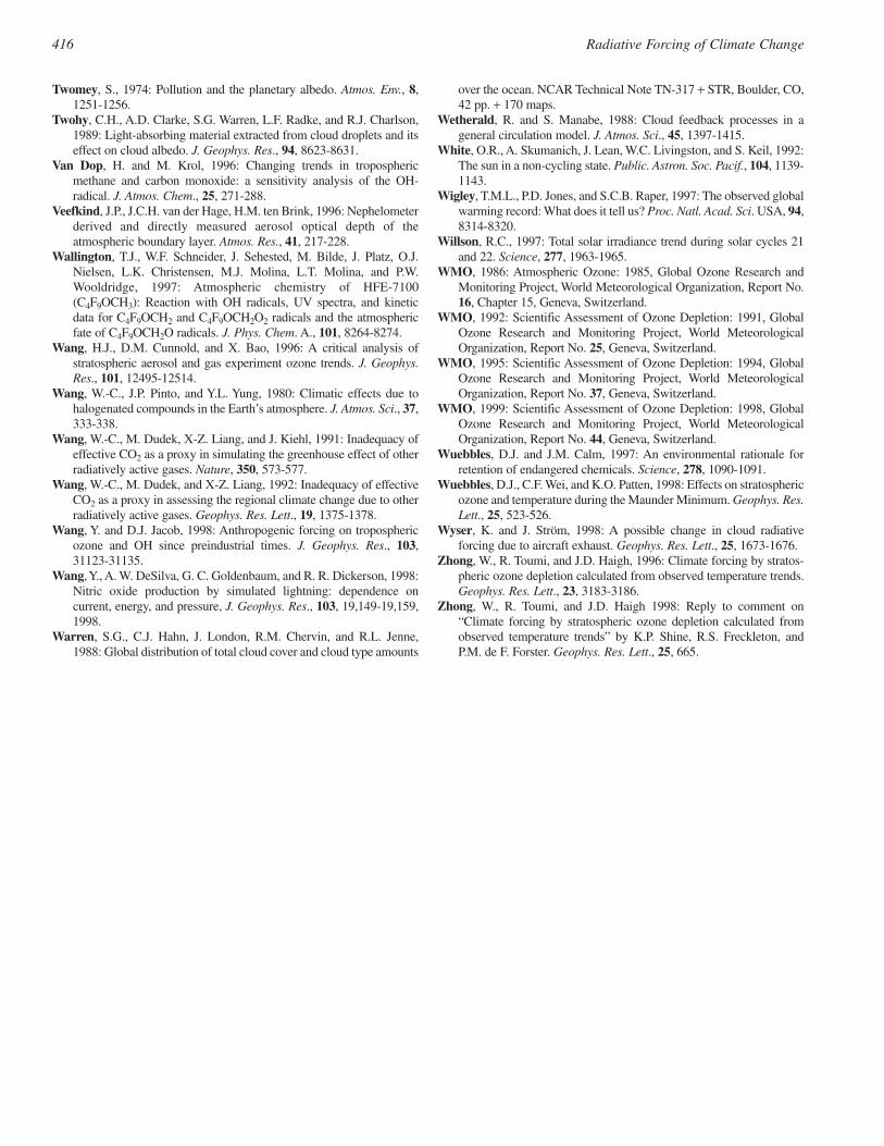
Twomey, S., 1974: Pollution and the planetary albedo. Atmos. Env., 8,1251-1256.
Twohy, C.H., A.D. Clarke, S.G. Warren, L.F. Radke, and R.J. Charlson,1989: Light-absorbing material extracted from cloud droplets and itseffect on cloud albedo. J. Geophys. Res., 94, 8623-8631.
Van Dop, H. and M. Krol, 1996: Changing trends in troposphericmethane and carbon monoxide: a sensitivity analysis of the OH-radical. J. Atmos. Chem., 25, 271-288.
Veefkind, J.P., J.C.H. van der Hage, H.M. ten Brink, 1996: Nephelometerderived and directly measured aerosol optical depth of theatmospheric boundary layer. Atmos. Res., 41, 217-228.
Wallington, T.J., W.F. Schneider, J. Sehested, M. Bilde, J. Platz, O.J.Nielsen, L.K. Christensen, M.J. Molina, L.T. Molina, and P.W.Wooldridge, 1997: Atmospheric chemistry of HFE-7100(C4F9OCH3): Reaction with OH radicals, UV spectra, and kineticdata for C4F9OCH2 and C4F9OCH2O2 radicals and the atmosphericfate of C4F9OCH2O radicals. J. Phys. Chem. A., 101, 8264-8274.
Wang, H.J., D.M. Cunnold, and X. Bao, 1996: A critical analysis ofstratospheric aerosol and gas experiment ozone trends. J. Geophys.Res., 101, 12495-12514.
Wang, W.-C., J.P. Pinto, and Y.L. Yung, 1980: Climatic effects due tohalogenated compounds in the Earth’s atmosphere. J. Atmos. Sci., 37,333-338.
Wang, W.-C., M. Dudek, X-Z. Liang, and J. Kiehl, 1991: Inadequacy ofeffective CO2 as a proxy in simulating the greenhouse effect of otherradiatively active gases. Nature, 350, 573-577.
Wang, W.-C., M. Dudek, and X-Z. Liang, 1992: Inadequacy of effectiveCO2 as a proxy in assessing the regional climate change due to otherradiatively active gases. Geophys. Res. Lett., 19, 1375-1378.
Wang, Y. and D.J. Jacob, 1998: Anthropogenic forcing on troposphericozone and OH since preindustrial times. J. Geophys. Res., 103,31123-31135.
Wang,Y., A. W. DeSilva, G. C. Goldenbaum, and R. R. Dickerson, 1998:Nitric oxide production by simulated lightning: dependence oncurrent, energy, and pressure, J. Geophys. Res., 103, 19,149-19,159,1998.
Warren, S.G., C.J. Hahn, J. London, R.M. Chervin, and R.L. Jenne,1988: Global distribution of total cloud cover and cloud type amounts
over the ocean. NCAR Technical Note TN-317 + STR, Boulder, CO,42 pp. + 170 maps.
Wetherald, R. and S. Manabe, 1988: Cloud feedback processes in ageneral circulation model. J. Atmos. Sci., 45, 1397-1415.
White, O.R., A. Skumanich, J. Lean, W.C. Livingston, and S. Keil, 1992:The sun in a non-cycling state. Public. Astron. Soc. Pacif., 104, 1139-1143.
Wigley, T.M.L., P.D. Jones, and S.C.B. Raper, 1997: The observed globalwarming record: What does it tell us? Proc. Natl. Acad. Sci. USA, 94,8314-8320.
Willson, R.C., 1997: Total solar irradiance trend during solar cycles 21and 22. Science, 277, 1963-1965.
WMO, 1986: Atmospheric Ozone: 1985, Global Ozone Research andMonitoring Project, World Meteorological Organization, Report No.16, Chapter 15, Geneva, Switzerland.
WMO, 1992: Scientific Assessment of Ozone Depletion: 1991, GlobalOzone Research and Monitoring Project, World MeteorologicalOrganization, Report No. 25, Geneva, Switzerland.
WMO, 1995: Scientific Assessment of Ozone Depletion: 1994, GlobalOzone Research and Monitoring Project, World MeteorologicalOrganization, Report No. 37, Geneva, Switzerland.
WMO, 1999: Scientific Assessment of Ozone Depletion: 1998, GlobalOzone Research and Monitoring Project, World MeteorologicalOrganization, Report No. 44, Geneva, Switzerland.
Wuebbles, D.J. and J.M. Calm, 1997: An environmental rationale forretention of endangered chemicals. Science, 278, 1090-1091.
Wuebbles, D.J., C.F. Wei, and K.O. Patten, 1998: Effects on stratosphericozone and temperature during the Maunder Minimum. Geophys. Res.Lett., 25, 523-526.
Wyser, K. and J. Ström, 1998: A possible change in cloud radiativeforcing due to aircraft exhaust. Geophys. Res. Lett., 25, 1673-1676.
Zhong, W., R. Toumi, and J.D. Haigh, 1996: Climate forcing by stratos-pheric ozone depletion calculated from observed temperature trends.Geophys. Res. Lett., 23, 3183-3186.
Zhong, W., R. Toumi, and J.D. Haigh 1998: Reply to comment on“Climate forcing by stratospheric ozone depletion calculated fromobserved temperature trends” by K.P. Shine, R.S. Freckleton, andP.M. de F. Forster. Geophys. Res. Lett., 25, 665.
416 Radiative Forcing of Climate Change