Radiative forcing by well-mixed greenhouse gases

Radiative forcing by well-mixed greenhouse gases:

Estimates from climate models in the

Intergovernmental Panel on Climate Change

(IPCC) Fourth Assessment Report (AR4)

W. D. Collins,1 V. Ramaswamy,2 M. D. Schwarzkopf,2 Y. Sun,3 R. W. Portmann,4

Q. Fu,5 S. E. B. Casanova,6 J.-L. Dufresne,7 D. W. Fillmore,8 P. M. D. Forster,9

V. Y. Galin,10 L. K. Gohar,6 W. J. Ingram,11 D. P. Kratz,12 M.-P. Lefebvre,7 J. Li,13

P. Marquet,14 V. Oinas,15 Y. Tsushima,16 T. Uchiyama,17 and W. Y. Zhong18

Received 26 September 2005; revised 11 February 2006; accepted 7 April 2006; published 28 July 2006.

[1] The radiative effects from increased concentrations of well-mixed greenhouse gases(WMGHGs) represent the most significant and best understood anthropogenic forcingof the climate system. The most comprehensive tools for simulating past and futureclimates influenced by WMGHGs are fully coupled atmosphere-ocean general circulationmodels (AOGCMs). Because of the importance of WMGHGs as forcing agents it isessential that AOGCMs compute the radiative forcing by these gases as accurately aspossible. We present the results of a radiative transfer model intercomparison betweenthe forcings computed by the radiative parameterizations of AOGCMs and bybenchmark line-by-line (LBL) codes. The comparison is focused on forcing by CO2, CH4,N2O, CFC-11, CFC-12, and the increased H2O expected in warmer climates. Themodels included in the intercomparison include several LBL codes and most of the globalmodels submitted to the Intergovernmental Panel on Climate Change (IPCC) FourthAssessment Report (AR4). In general, the LBL models are in excellent agreement witheach other. However, in many cases, there are substantial discrepancies among theAOGCMs and between the AOGCMs and LBL codes. In some cases this is because theAOGCMs neglect particular absorbers, in particular the near-infrared effects of CH4 andN2O, while in others it is due to the methods for modeling the radiative processes. The biasesin the AOGCM forcings are generally largest at the surface level. We quantify thesedifferences and discuss the implications for interpreting variations in forcing and responseacross the multimodel ensemble of AOGCM simulations assembled for the IPCC AR4.

Citation: Collins, W. D., et al., (2006), Radiative forcing by well-mixed greenhouse gases: Estimates from climate models in the

Intergovernmental Panel on Climate Change (IPCC) Fourth Assessment Report (AR4), J. Geophys. Res., 111, D14317,

doi:10.1029/2005JD006713.

1. Introduction

[2] One of the major factors underlying recent climatechange is radiative forcing. Radiative forcing is an exter-nally imposed change in the radiative energy budget of the

Earth’s climate system [Intergovernmental Panel on ClimateChange (IPCC), 2001]. The energy budget is characterizedby an approximate balance between shortwave absorptionand longwave emission by the climate system [e.g., Kiehl

JOURNAL OF GEOPHYSICAL RESEARCH, VOL. 111, D14317, doi:10.1029/2005JD006713, 2006ClickHere

for

FullArticle

1National Center for Atmospheric Research, Boulder, Colorado, USA.2Geophysical Fluid Dynamics Laboratory, Princeton, New Jersey, USA.3National Climate Center, Beijing, China.4Aeronomy Laboratory, NOAA, Boulder, Colorado, USA.5Department of Atmospheric Sciences, University of Washington,

Seattle, Washington, USA.6Department of Meteorology, University of Reading, Reading, UK.7Laboratoire de Meteorologie Dynamique, Paris, France.8Le Laboratoire des Sciences du Climat et l’Environnement, Gif-sur-

Yvette, France.9School of Earth and Environment, University of Leeds, Leeds, UK.

Copyright 2006 by the American Geophysical Union.0148-0227/06/2005JD006713$09.00

D14317

10Institute of Numerical Mathematics, Academy of Sciences, Moscow,Russia.

11Department of Physics, Clarendon Laboratory, Oxford, UK.12NASA Langley Research Center, Hampton, Virginia, USA.13Canadian Centre for Climate Modeling and Analysis, University of

Victoria, Victoria, British Columbia, Canada.14Meteo-France, CNRM, Toulouse, France.15NASA Goddard Institute for Space Studies, New York, New York,

USA.16Frontier Research Center for Global Change, Japan Agency for

Marine-Earth Science and Technology, Yokohama, Japan.17Meteorological Research Institute, Tsukuba, Japan.18Physics Department, Imperial College, London, UK.

1 of 15

http://dx.doi.org/10.1029/2005JD006713

and Trenberth, 1997]. Radiative forcing can affect eitherthe shortwave or longwave components of the radiativebudget. The changes can be caused by a number of factorsincluding variations in solar insolation, alteration in surfaceboundary conditions related to land use change and desert-ification, or natural and anthropogenic perturbations to theradiatively active species in the atmosphere. The most basicand most important forcings are related to anthropogenicincreases in the well-mixed greenhouse gases (WMGHGs)CO2, CH4, N2O, and the halocarbons. The WMGHGsenhance the absorption of radiation in the atmospherethrough excitation of molecular rotational and rotational-vibrational modes by infrared and near-infrared photons.Despite continuing uncertainty regarding the magnitudeof aerosol radiative forcing [Anderson et al., 2003], it isvery likely that the net anthropogenic radiative forcing ofthe climate system is positive because of the effects ofWMGHGs [Boucher and Haywood, 2001]. The increasedconcentrations of CO2, CH4, and N2O between 1750and 1998 have produced forcings of +1.48, +0.48, and+0.15 W m�2, respectively [IPCC, 2001]. The introductionof halocarbons in the mid-20th century has contributed anadditional +0.34 W m�2, for a total forcing by WMGHGs of+2.45Wm�2 with a 15%margin of uncertainty. The positivesign of these forcings reflects the fact that the climate systemis releasing less and absorbing more radiative energy than inits unperturbed state.[3] Coupled atmosphere-ocean general circulation mod-

els (AOGCMs) [Trenberth, 1992; Randall, 2000] representthe most comprehensive systems for simulating the re-sponse of the climate to radiative forcings. AOGCMs havebeen used extensively to simulate change in response toWMGHGs and other agents since pioneering studies byManabe and Wetherald [1975] and other modeling groups.In the current fourth Assessment Report (AR4) of theIntergovernmental Panel on Climate Change (IPCC), six-teen international groups are submitting simulations from23 different AOGCMs. These simulations are used toproject climate change in the recent past and in the futureunder a variety of emissions scenarios for WMGHGs andother radiative species [Nakicenovic and Swart, 2000].[4] Because of the intrinsic complexity of the numerous

processes included in these models and the computationaldemands of climate change simulation, it is frequentlynecessary to approximate the various processes using sim-plified representations called parameterizations. Suchapproximations are necessary both for processes groundedin first principles theory (e.g., radiative transfer) and forelements of the climate system which are less well under-stood (e.g., clouds). Radiative transfer is one physicalprocess that can be calibrated against fiduciary methods inthe form of highly accurate numerical solutions. Thesesolutions can be employed to verify parameterizations ofradiative effects in climate models. The lack of stringentobservational or theoretical constraints on the second classof processes has resulted in a diversity of parameterizationsfor many components of the climate system. The use of amultimodel ensemble in the IPCC assessment reports is anattempt to characterize the impact of parameterizationuncertainty on climate change predictions.[5] The interaction of shortwave and longwave radiation

with an (idealized) atmosphere free of clouds and aerosols

can be calculated to a very high degree of accuracy[Halthore et al., 2005]. The remaining uncertainties arerelated primarily to some aspects of the spectroscopy of theWMGHGs and other atmospheric constituents and to thetreatment of broadband continuum absorption by H2O, CO2,and other species. Very accurate line-by-line (LBL) codescan solve the basic equations of radiative transfer [Liou,1992] for each quantum transition, or ‘‘line’’, registered foreach radiatively active molecular constituent in the atmo-sphere. In carefully controlled comparisons against fielddata, LBL results agree with measured spectra to withinobservational uncertainty [e.g., Tjemkes et al. 2003], al-though this agreement is, to some extent, due to empiricaltuning of the water vapor continuum. Kratz et al. [2005]have shown that a collection of LBL models produce far-infrared radiances and fluxes that differ by roughly 0.5%when applied to identical atmospheric profiles. The resultsfrom LBL codes represent a rigorous set of benchmarkcalculations for development and evaluation of radiationcodes in AOGCMs [Clough and Iacono, 1995].[6] There have been several efforts to evaluate the accu-

racy of radiative parameterizations in AOGCMs relative toLBL calculations. The major projects include the Intercom-parison of Radiation Codes in Climate Models (ICRCCM)[Ellingson and Fouquart, 1991; Ellingson et al., 1991;Fouquart et al., 1991], an intercomparison of forcing byozone computed with various codes [Shine et al., 1995], theGCM Reality Intercomparison Project for SPARC (GRIPS)[Pawson et al., 2000], an assessment of treatments forunresolved clouds [Barker et al., 2003], and an intercom-parison of shortwave codes and measurements [Halthore etal., 2005]. Heating rates have been previously evaluated byFels et al. [1991]. Analysis of radiative forcing byWMGHGs derived from earlier generations of AOGCMshas uncovered large discrepancies relative to LBL calcu-lations, for example in the forcing from doubling atmo-spheric concentrations of CO2 [Cess et al., 1993]. Theproblems encountered in the Cess et al. [1993] studyinclude omission of minor CO2 absorption bands, errorsin the overlap of absorption by H2O and CO2, and unre-solved issues with the formulation of longwave radiativetransfer. Analyses of the radiative forcing by sulfate aero-sols has also demonstrated large differences among models[Boucher et al., 1998].[7] In this study, we update the earlier intercomparisons

by evaluating many of the AOGCMs included in the IPCCAR4 (2007) (in preparation) against a representative set ofcurrent LBL codes. The goals of this exercise are to evaluatethe fidelity of AOGCMs included in the IPCC AR4 and toestablish new benchmark calculations for this purpose. Thechief objective is to determine the differences in WMGHGforcing caused by the use of different radiation codes in theAOGCMs used for IPCC simulations of climate change.Unlike some of the previous studies, the emphasis here is onthe accuracy of radiative forcing rather than radiative flux.While the effects of increasing WMGHGs represent onlypart of the forcing applied to the climate system, a compre-hensive evaluation of all the forcing agents in AOGCMs isbeyond the scope of this work.[8] The Radiative Transfer Model Intercomparison Proj-

ect (RTMIP) and the participating models are described insection 2. Results for the radiative forcings at the top of

D14317 COLLINS ET AL.: GREENHOUSE FORCING BY AOGCMS IN IPCC AR4

2 of 15

D14317

model (TOM), 200 hPa (a surrogate for the tropopause), andsurface are presented in section 3.1. A comparison of thecorresponding changes in atmospheric heating rates is givenin section 3.2. Discussion and conclusions are presented insection 4.

2. Experimental Configuration

2.1. Clear-Sky Forcing Calculations

[9] The specific goal of this study is to quantify thedifferences in instantaneous radiative forcing calculatedfrom AOGCM and LBL radiation codes. On the basis ofexperience from previous intercomparisons, the calculationsrequested from the participants in RTMIP are not sufficientfor detailed explanation of the differences. On the otherhand, minimizing the number of required calculations hashelped insure nearly unanimous participation by theAOGCM groups.[10] The calculations are performed off line by applying

the LBL codes and radiative parameterizations from theAOGCMs to a specified atmospheric profile. The results aretherefore not affected by differences among the atmosphericclimatologies produced by the various AOGCMs. Theradiatively active species included in this evaluation arethe WMGHGs CO2, CH4, N2O, and the chlorofluorocar-bons CFC-11 and CFC-12. The intercomparison is basedupon calculations of the instantaneous changes in clear-skyfluxes when concentrations of these WMGHGs are per-turbed. While the relevant quantity for climate change is all-sky forcing, the introduction of clouds would greatlycomplicate the intercomparison exercise and thereforeclouds are omitted from RTMIP.[11] In addition, the calculations omit the effects of

stratospheric thermal adjustment to forcing derived usingfixed dynamical heating (FDH) [Ramanathan andDickinson, 1979; Fels et al., 1980]. This omission facilitates

comparison of fluxes from LBL codes and AOGCM param-eterizations. For the purposes of this intercomparison, ‘‘flux’’is defined as ‘‘flux for clear-sky and aerosol-free conditions’’and ‘‘forcing’’ is defined as ‘‘instantaneous changes in fluxeswithout stratospheric adjustment’’. It should be noted that ouromission of FDH means that the results in this study are notdirectly comparable to the estimates of forcing at the tropo-pause in the IPCC [2001] reports, since the latter include theeffects of adjustment. The effects of adjustment on forcingare approximately �2% for CH4, �4% for N2O, +5% forCFC-11, +8% for CFC-12, and�13% for CO2 [IPCC, 1995;Hansen et al., 1997].[12] The specifications for each of the calculations

requested from the LBL and AOGCM groups are given inTable 1. The concentrations of WMGHGs in calculations 3aand 3b correspond to conditions in the years 1860 AD and2000 AD, respectively. The concentrations in 1860 areobtained from a variety of sources detailed in IPCC[2001]. Differences among these calculations cover severalstandard forcing scenarios performed by all AOGCMs inthe AR4, including (1) forcing for changes in CO2 concen-trations from 1860 to 2000 values (case 2a-1a) and from1860 to double 1860 values (case 2b-1a), (2) forcingfor changes in WMGHGs from 1860 to 2000 values(case 3b-3a), and (3) the effect of increased H2O predictedwhen CO2 is doubled (case 4a-2b). In addition to the fourforcing experiments listed above, there are three additionalforcing experiments for combinations of CH4, N2O, CFC-11,and CFC-12. The changes in WMGHGs and H2O inthese seven forcing experiments are listed in Table 2.[13] The quantities requested from each participating

group include (1) net shortwave and longwave clear-skyflux at the top of the model, (2) net shortwave and longwaveclear-sky flux at 200 hPa, (3) net shortwave and longwaveclear-sky flux at the surface, and (4) (optionally) netshortwave and longwave clear-sky fluxes at each layerinterface in the profile. The reason for performing calcu-lations at 200 hPa rather than the tropopause is to insureconsistency with the radiative quantities requested as part ofthe climate change simulations. Since not all modelinggroups are prepared to compute fluxes at a time-evolvingtropopause, the Working Group on Coupled Modeling(WGCM) of the World Climate Research Programme(WCRP) and the IPCC have requested fluxes at a surrogatefor the tropopause at the 200 hPa pressure surface. Theprecise choice of tropopause can affect forcings by up to10% [Myhre and Stordal, 1997].[14] In order to establish a common baseline, the back-

ground atmospheric state for all the calculations is a

Table 1. Atmospheric Constituents for the Radiative Calculations

CalculationCO2,ppmv

CH4,ppbv

N2O,ppbv

CFC-11,pptv

CFC-12,pptv H2O

a

1a 287 0 0 0 0 12a 369 0 0 0 0 12b 574 0 0 0 0 13a 287 806 275 0 0 13b 369 1760 316 267 535 13c 369 1760 275 0 0 13d 369 806 316 0 0 14a 574 0 0 0 0 1.2

aMultiplier applied to the H2O mixing ratios in the AFGL MLS profile.

Table 2. Changes in Atmospheric Constituents for Forcing Calculations

Casea CO2, ppmv CH4, ppbv N2O, ppbv CFC-11, pptv CFC-12, pptv H2Ob

2a-1a 287 ! 369 – – – – –2b-1a 287 ! 574 – – – – –3b-3a 287 ! 369 806 ! 1760 275 ! 316 0 ! 267 0 ! 535 –3a-1a – 0 ! 806 0 ! 275 – – –3b-3c – – 275 ! 316 0 ! 267 0 ! 535 –3b-3d – 806 ! 1760 – 0 ! 267 0 ! 535 –4a-2b – – – – – 1 ! 1.2

aDifferences between calculations in Table 1.bChange in multiplier applied to the H2O mixing ratios in the AFGL MLS profile.


3 of 15

D14317

climatological midlatitude summer (MLS) atmospheric pro-file [Anderson et al., 1986]. Therefore all the calculationsare performed using the same vertical profiles of tempera-ture and the mixing ratio of O3. The profile of specifichumidity is also held fixed except for calculation 4a(Table 1). The concentrations of WMGHGs are set to aconstant mixing ratio with respect to dry air throughout thecolumn. The standard MLS profile has been interpolated to40 levels for the AOGCM groups and 459 levels for theLBL groups. As shown in Table 3, the comparison offorcings from AOGCM and LBL codes is not affected bythe difference in resolution. Increasing resolution from 40 to459 levels changes the longwave forcings at TOM andsurface by less than approximately 0.01 W m�2. Changingthe methods of temperature interpolation within each layerin the LBL calculations changes the longwave forcings byless than 0.02 W m�2. The input profiles are available fromthe RTMIP Web site at http://www.cgd.ucar.edu/RTMIP/.[15] The main radiative effects of atmospheric species

included in the calculations are molecular Rayleigh scatter-ing and the absorption by the WMGHGs, H2O, and O3.There is also a reduction in O2 stoichiometrically equivalentto the increase in CO2. The forcing calculations should notbe appreciably affected by the red and near-infrared (A, B,and g) bands of O2, collisionally induced rotation bands inN2 at approximately 100 mm, quadrupole transitions in thefundamental vibration band of N2 at 4.3 mm, the forbiddentransitions of O2 in the vibration-rotation band, or thecollision complexes O2 � O2 and O2 � N2. For example,the effect of the A, B, and g bands of O2 on the shortwaveforcing is less than 0.001 W m�2 (Table 3). The inclusion or

omission of these absorption bands has been left to thediscretion of the individual AOGCM and LBL modelers.The LBL groups have used spectral ranges of 4 to 100 mmfor the longwave and 0.2 to 5 mm for the shortwave. Thespectral interval of 4 to 5 mm is contained in both shortwaveand longwave calculations, but it is not counted twice sincethe shortwave codes omit thermal emission and the long-wave codes omit solar flux. Some of the LBL groups haveprovided their spectrally resolved fluxes corresponding totheir broadband calculations. The AOGCM groups havebeen asked to use the standard spectral ranges for theirrespective radiative parameterizations.[16] For the shortwave calculations, the surface is a

Lambertian reflector with a spectrally flat albedo of 0.1.At the TOM, the solar radiation is set to 1360 W m�2

incident at a zenith angle of 53 degrees. The value for TOMsolar insolation is the difference between a broadband solarconstant of 1367 W m�2 and the 6.33 W m�2 of insolationin wavelengths larger than 5 mm excluded from the calcu-lations [Labs and Neckel, 1970]. This radiation is excludedsince most AOGCM shortwave parameterizations do nottreat this wavelength range. For the longwave calculations,the surface is assumed to have a spectrally flat emissivityequal to 1 and a thermodynamic temperature of 294 K.

2.2. General Circulation and Line-by-Line Models

[17] The AOGCM groups and models contributing cal-culations to RTMIP are listed in Tables 4 and 5. There are16 groups submitting simulations to the IPCC AR4, andfourteen of these are participating in RTMIP. The groupshave submitted simulations from 23 models to the IPCC

Table 3. Sensitivity of TOM and Surface Forcings to Features of the Calculationsa

Band Feature hdFTOM(Band)i, W m�2 hdFSRF(Band)i, W m�2

LW vertical resolution �0.011 ± 0.017 �0.004 ± 0.009LW temperature interpolation 0.011 ± 0.020 0.016 ± 0.013SW O2 absorption 0.000 ± 0.001 0.001 ± 0.003aParameters hdFTOM(Band)i and hdFSRF(Band)i are the mean changes in TOM and surface forcing when features of the forcing calculation are changed.

The mean changes are averages across the seven forcing cases listed in Table 2. The longwave (LW) sensitivities are calculated using the NASA MRTAmodel (Table 6), and the shortwave (SW) sensitivities are calculated using the NCAR CCSM3 radiative parameterization (Table 4).

Table 4. AOGCMs in the Intercomparison

Originating Groupa Country Model

BCCR Norway BCCR-BCM2.0CCCma Canada CGCM3.1(T47/T63)CCSR/NIES/FRCGC Japan MIROC3.2(medres/hires)CNRM France CNRM-CM3GFDL USA GFDL-CM2.0/2.1GISS USA GISS-EH/ERINM Russia INM-CM3.0IPSL France IPSL-CM4LASG/IAP China FGOALS-g1.0MIUB/METRI/KMA Germany/Korea ECHO-GMPIfM Germany ECHAM5/MPI-OMMRI Japan MRI-CGCM2.3.2NCAR USA CCSM3NCAR USA PCMUKMO UK HadCM3UKMO UK HadGEM1

aThe acronyms for the groups are given in Table 5.


4 of 15

D14317

data archive, and calculations representing twenty of theseare included in our intercomparison. It should be noted thata number of the AOGCMs have similar or identical radia-tive parameterizations. The two AOGCMs developed byeach of the groups CCCma, CCSR/NIES/FRCGC, GFDL,and GISS share common radiation codes. Each pair ofmodels is represented by a single set of calculations inRTMIP. In addition, the models BCCR-BCM2.0 andCNRM-CM3 have identical parameterizations, and thetreatments of trace gases in CCSM3, FGOALS-g1.0 andPCM are essentially the same. The characteristics of theradiative parameterizations used in many of these AOGCMsare described in detail by Q. Fu and V. Ramaswamy(manuscript in preparation, 2006).[18] The LBL groups contributing calculations to RTMIP

are listed in Tables 5 and 6. The details of the calculationsperformed with each LBL code are given in Table 7. Thefive participating LBL groups have each performed thelongwave calculations, and four excepting LARC haveperformed the shortwave calculations. The LBL modelsare all based upon the same Hitran line database forradiatively active species [Rothman et al., 2003], althoughthree of the models include additional corrections to thatdatabase. Because of the heterogeneity of LBL configura-tions shown in Table 7, the agreement among the absolutefluxes from these codes is not as good as the agreement thatcan be achieved in more rigorously controlled intercompar-isons [e.g., Kratz et al., 2005]. However, the objective inRTMIP is to derive accurate forcings, and the set of LBL

calculations is adequate for that application (section 3). Thereason is that any offsets in the fluxes from a particular LBLcode are sufficiently constant across the various calculationsthat the offsets cancel when differencing these calculationsto derive the forcings. For example, consider the 200 hPalongwave fluxes F200(LW) for calculations 1a and 2a. Thedifference between these fluxes is the longwave forcing at200 hPa caused by an increase in CO2 from 287 to369 ppmv (Table 2). For both of the calculations 1a and2a, the standard deviation of the five LBL estimates ofF200(LW) is 1.25 W m�2. However, the standard deviationof the forcing (the difference between calculations 1aand 2a) is just 0.02 Wm�2. This example illustrates thatdiscrepancies among LBL radiative codes that affect thecalculation of fluxes need not appreciably affect the calcu-lation of forcings. The results from the LBL codes areavailable from the RTMIP Web site at http://www.cgd.u-car.edu/RTMIP/.[19] Sample longwave forcing calculations with the Ref-

erence Forward Model (RFM) (Tables 6 and 7) are shown inFigure 1. The ratio of the net longwave flux at 200 hPa tothe longwave upward flux from the surface is plotted inFigure 1 (top). Values close to 1 indicate that radiationreaching 200 hPa originates from the surface or near thesurface, while values close to 0 result from a combination ofstrong absorption and the thermal stratification of thetroposphere [Goody and Yung, 1989]. The four prominentfeatures are the strong H2O band at 6.3 mm, the midinfrared‘‘window’’ between 8 and 12 mm, the CO2 band at 15 mm,

Table 5. Acronyms for Modeling Groups

Acronym Originating Group

BCCR Bjerknes Centre for Climate ResearchCCCma Canadian Centre for Climate Modeling and AnalysisCCSR Center for Climate System Research (The University of Tokyo)CNRM Centre National de Recherches Meteorologiques (Meteo-France)FRCGC Frontier Research Center for Global Change (JAMSTEC)GFDL Geophysical Fluid Dynamics Laboratory (NOAA)GISS Goddard Institute for Space Studies (NASA)IAP Institute of Atmospheric PhysicsICSTM Imperial College of Science, Technology, and MedicineINM Institute for Numerical MathematicsIPSL Institut Pierre Simon LaplaceJAMSTEC Japan Agency for Marine-Earth Science and TechnologyLARC Langley Research Center (NASA)LASG Laboratory of Numerical Modeling for Atmospheric

Sciences and Geophysical Fluid DynamicsMPIfM Max Planck Institute for MeteorologyMRI Meteorological Research InstituteMIUB Meteorological Institute of the University of BonnMETRI/KMA Meteorological Research Institute, Korean

Meteorological AdministrationNCAR National Center for Atmospheric ResearchNIES National Institute for Environmental StudiesUKMO Met Office’s Hadley Centre for Climate Prediction and ResearchUR University of Reading

Table 6. LBL Radiation Codes in the Intercomparison

Originating Groupa Country Model Reference

GFDL USA GFDL LBL Schwarzkopf and Fels [1985]GISS USA LBL3 –ICSTM UK GENLN2 Edwards [1992]; Zhong et al. [2001]LARC USA MRTA Kratz and Rose [1999]UR UK RFM Dudhia [1997] and Stamnes et al. [1988]

aThe acronyms for the groups are given in Table 5.


5 of 15

D14317

and the far-infrared rotation band of H2O [Liou, 1992]. Thelongwave forcings for four of the experiments in Table 2 areplotted in Figure 1 (bottom). As Figure 1 illustrates, thelargest forcings generally occur outside the band centers ofthe major absorbing species. For example, the largest CO2

forcings appear in the wings of the 15 mm band [e.g., IPCC1995, Figure 4.1]. Similarly, the largest H2O forcings occurin the midinfrared window and the far infrared, not in the6.3 mm H2O band. The reason is that the absorption in theband centers is effectively saturated, and therefore increasesin radiatively active species have minimal effects at thosewavelengths.[20] Corresponding shortwave forcing calculations per-

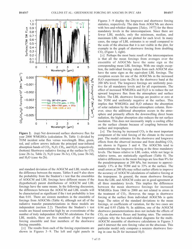
formed with the RFM are shown in Figure 2. The ratio ofthe net surface flux to the TOM solar radiation is plotted inFigure 2 (top). At wavelengths where the ratio is close to 1,the atmosphere transmits most of the incident flux to thesurface [Goody and Yung, 1989]. Where the ratio is close to0, the incident flux is largely absorbed by trace gases andwater vapor along the ray path from the top of atmosphereto the surface. The major features in the transmissionspectrum are the extremely strong O3 bands at wavelengthsbelow 0.26 mm, the visible atmospheric ‘‘window’’ between0.3 and 0.7 mm, the CO2 bands at 2.7 and 4.3 mm, and theprimary and overtone bands of H2O [Liou, 1992]. Theshortwave forcings for four of the experiments in Table 2are plotted in Figure 2 (right). Because of saturation effects,there is virtually no forcing near the CO2 and H2O bandcenters at 2.7 mm or the middle of the CO2 band at 4.3 mm.However, in other near-infrared bands of H2O and theWMGHGs, the line strengths are sufficiently weak thatforcing can occur near the band centers. An example isthe forcing by H2O in its overtone bands at wavelengthsbelow 2 mm [Ramaswamy and Freidenreich, 1998]. It isalso evident from comparison of the ordinates in Figures 1(right) and 2 (right) that the forcings by WMGHGs in thenear infrared are generally weaker than the forcings in themiddle and far infrared.

3. Comparison of Calculations from AOGCMsand LBL Models

3.1. Forcings From AOGCMs and LBL Models

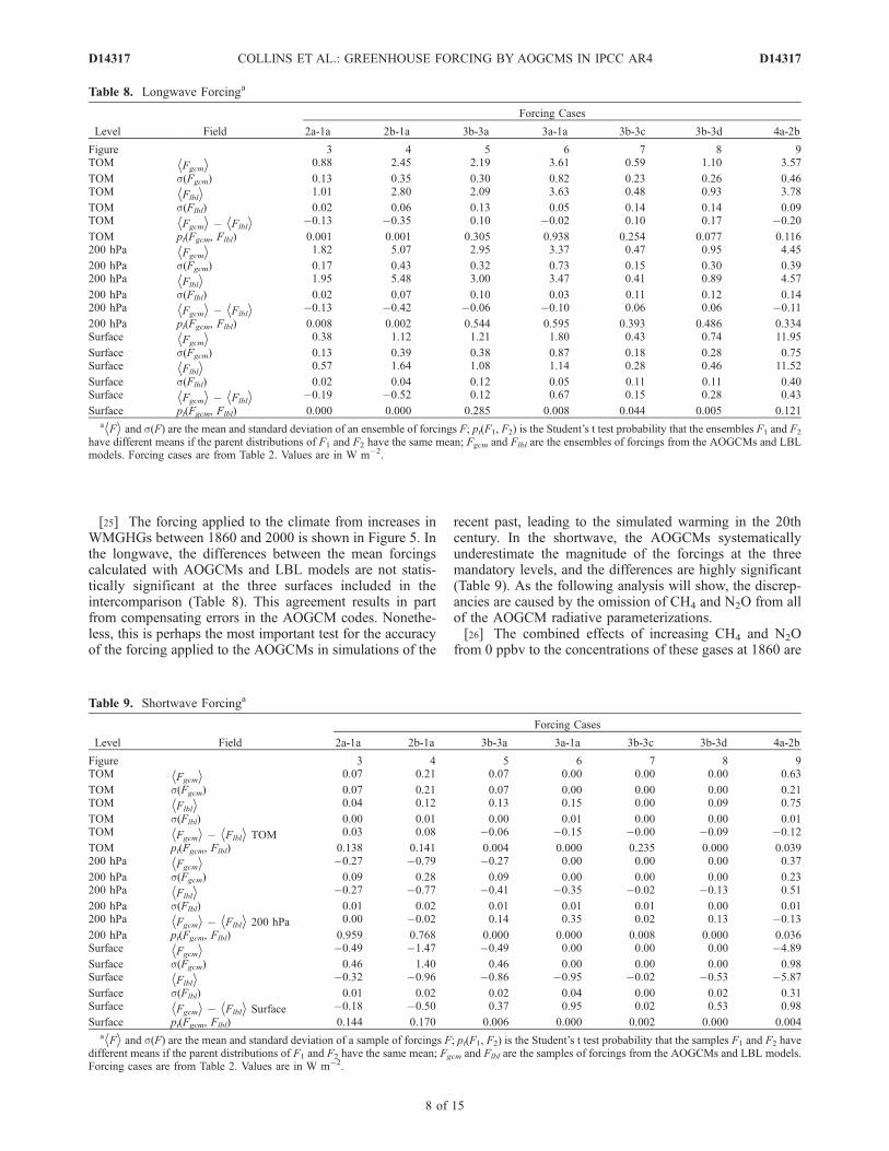
[21] The statistical summaries of the forcing intercompar-ison are given in Table 8 for the longwave and Table 9 forthe shortwave. For each level, Tables 8 and 9 list the mean

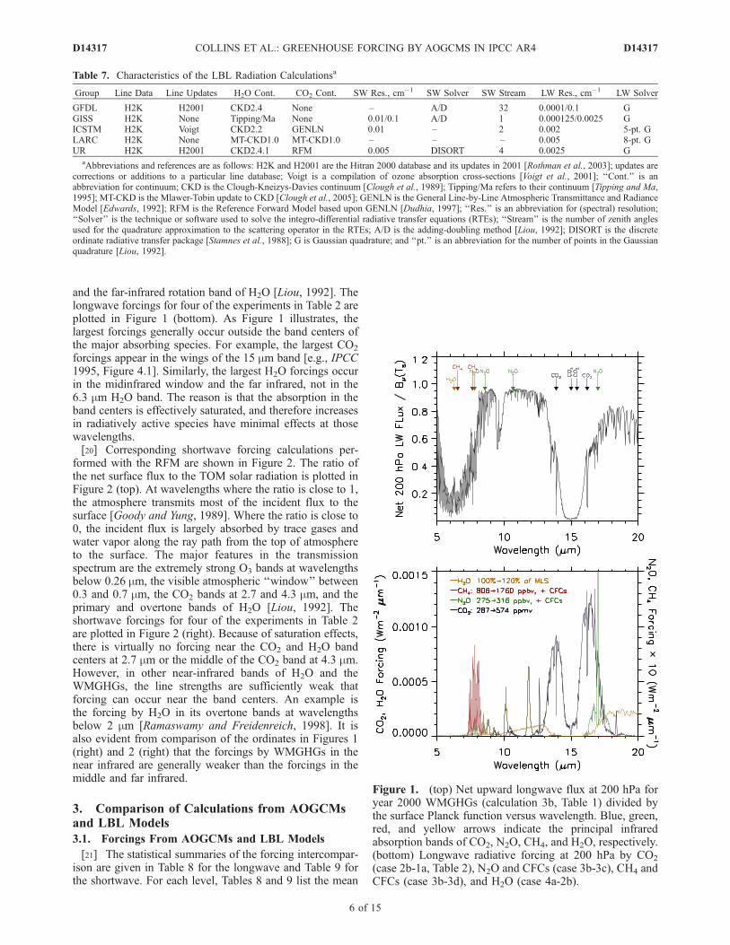
Table 7. Characteristics of the LBL Radiation Calculationsa

Group Line Data Line Updates H2O Cont. CO2 Cont. SW Res., cm�1 SW Solver SW Stream LW Res., cm�1 LW Solver

GFDL H2K H2001 CKD2.4 None – A/D 32 0.0001/0.1 GGISS H2K None Tipping/Ma None 0.01/0.1 A/D 1 0.000125/0.0025 GICSTM H2K Voigt CKD2.2 GENLN 0.01 – 2 0.002 5-pt. GLARC H2K None MT-CKD1.0 MT-CKD1.0 – – – 0.005 8-pt. GUR H2K H2001 CKD2.4.1 RFM 0.005 DISORT 4 0.0025 G

aAbbreviations and references are as follows: H2K and H2001 are the Hitran 2000 database and its updates in 2001 [Rothman et al., 2003]; updates arecorrections or additions to a particular line database; Voigt is a compilation of ozone absorption cross-sections [Voigt et al., 2001]; ‘‘Cont.’’ is anabbreviation for continuum; CKD is the Clough-Kneizys-Davies continuum [Clough et al., 1989]; Tipping/Ma refers to their continuum [Tipping and Ma,1995]; MT-CKD is the Mlawer-Tobin update to CKD [Clough et al., 2005]; GENLN is the General Line-by-Line Atmospheric Transmittance and RadianceModel [Edwards, 1992]; RFM is the Reference Forward Model based upon GENLN [Dudhia, 1997]; ‘‘Res.’’ is an abbreviation for (spectral) resolution;‘‘Solver’’ is the technique or software used to solve the integro-differential radiative transfer equations (RTEs); ‘‘Stream’’ is the number of zenith anglesused for the quadrature approximation to the scattering operator in the RTEs; A/D is the adding-doubling method [Liou, 1992]; DISORT is the discreteordinate radiative transfer package [Stamnes et al., 1988]; G is Gaussian quadrature; and ‘‘pt.’’ is an abbreviation for the number of points in the Gaussianquadrature [Liou, 1992].

Figure 1. (top) Net upward longwave flux at 200 hPa foryear 2000 WMGHGs (calculation 3b, Table 1) divided bythe surface Planck function versus wavelength. Blue, green,red, and yellow arrows indicate the principal infraredabsorption bands of CO2, N2O, CH4, and H2O, respectively.(bottom) Longwave radiative forcing at 200 hPa by CO2

(case 2b-1a, Table 2), N2O and CFCs (case 3b-3c), CH4 andCFCs (case 3b-3d), and H2O (case 4a-2b).


6 of 15

D14317

and standard deviation of the AOGCM and LBL results andthe difference between the means. Tables 8 and 9 also showthe probability from the Student’s t test that the ensemblesof AOGCM and LBL forcings have different means if the(hypothetical) parent distributions of AOGCM and LBLforcings have the same means. In the following discussion,the differences between the AOGCM and LBL results willbe characterized as significant if the t test probability is lessthan 0.01. There are sixteen members in the ensemble offorcings from AOGCMs (Table 4), although not all of theradiative transfer parameterizations in these models areindependent (section 2.2). Therefore the Student’s t testresults are biased somewhat high by an overestimate of thenumber of truly independent AOGCM calculations. For theLBL models, there are five members of the longwaveforcing ensemble and four members of the shortwaveforcing ensemble.[22] The results from each of the forcing experiments are

shown in Figures 3–9. The left and right panels in

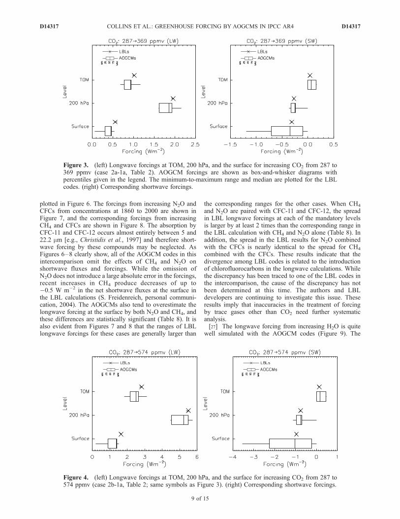
Figures 3–9 display the longwave and shortwave forcingstatistics, respectively. The data from AOGCMs are shownwith box-and-whisker diagrams [Tukey, 1977] for the threemandatory levels in the intercomparison. Since there arefewer LBL models, only the minimum, median, andmaximum LBL values are plotted for each level. In manycases, the range of LBL estimates is so small compared tothe scale of the abscissa that it is not visible in the plot, forexample in the graph of shortwave forcing from doublingCO2 (Figure 3, right).[23] Perhaps the most basic result of the intercomparison

is that all the mean forcings from averages over theensemble of AOGCMs have the same sign as thecorresponding mean LBL forcings. With one single excep-tion, the individual forcing values from each AOGCM alsohave the same signs as the equivalent LBL forcings. Theexception occurs for one of the AOGCMs in the increasedH2O experiment (case 4a-2b) in the shortwave band at the200 hPa level. The longwave forcings are uniformly posi-tive for all mandatory levels and for all experiments. Theeffect of increased WMGHGs and H2O is to reduce the netupward longwave flux from the atmosphere and surfacebelow. The LBL shortwave forcings are positive or zero atthe TOM and uniformly negative at the surface. Thisimplies that WMGHGs and H2O enhance the absorptionof solar radiation by the surface-atmosphere column. How-ever, since the additional absorption occurs in the atmo-sphere and primarily affects the downwelling direct beamradiation, the higher absorption also reduces the net surfaceinsolation. This does not necessarily imply a cooling effecton the surface climate because of coupling between thesurface and troposphere.[24] The forcing by increased CO2 is the most important

component of the total forcing of the climate in the recentpast. The model estimates for the shortwave and longwaveeffects from the observed increase and from doubling CO2

are shown in Figures 3 and 4. The AOGCMs tend tounderestimate the longwave forcing at the three mandatorylevels. The biases relative to LBL codes, while not large inrelative terms, are statistically significant (Table 8). Therelative differences in the mean forcings are less than 8% forthe pseudotropopause at 200 hPa, but increase to approxi-mately 13% at the TOM and to 33% at the surface. Thesmall errors at 200 hPa may reflect earlier efforts to improvethe accuracy of AOGCM calculations of radiative forcing atthe tropopause. In general, the mean shortwave forcingsfrom the LBL and AOGCM codes are in good agreement atall three mandatory levels. This implies the differencesbetween the mean shortwave forcings for increasedWMGHGs from 1860 to 2000 are not related to errors inthe treatment of CO2. However, the range in shortwaveforcing at the surface from individual AOGCMs is quitelarge. The ratios of the standard deviations to the meanforcings, or coefficients of variation, for the two cases are0.94 and 0.95 (Table 9). In addition, one of the AOGCMshortwave parameterizations does not include the effects ofCO2 on shortwave fluxes and heating rates. The omissionexplains why the box-and-whisker diagrams for the multi-AOGCM ensemble of shortwave calculations in Figures 3and 4 intersect the zero forcing value on the abscissas. Thisparticular model only computes a nonzero shortwave forc-ing in case 4a-2b for increased H2O.

Figure 2. (top) Net downward surface shortwave flux foryear 2000 WMGHGs (calculation 3b, Table 1) divided byTOM incident solar flux versus wavelength. Blue, green,red, and yellow arrows indicate the principal near-infraredabsorption bands of CO2, N2O, CH4, and H2O, respectively.(bottom) Shortwave radiative forcing at the surface by CO2

(case 2b-1a, Table 2), N2O (case 3b-3c), CH4 (case 3b-3d),and H2O (case 4a-2b).


7 of 15

D14317

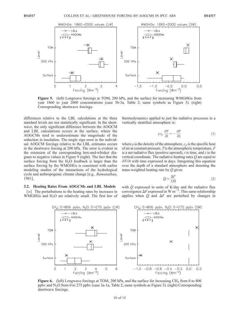
[25] The forcing applied to the climate from increases inWMGHGs between 1860 and 2000 is shown in Figure 5. Inthe longwave, the differences between the mean forcingscalculated with AOGCMs and LBL models are not statis-tically significant at the three surfaces included in theintercomparison (Table 8). This agreement results in partfrom compensating errors in the AOGCM codes. Nonethe-less, this is perhaps the most important test for the accuracyof the forcing applied to the AOGCMs in simulations of the

recent past, leading to the simulated warming in the 20thcentury. In the shortwave, the AOGCMs systematicallyunderestimate the magnitude of the forcings at the threemandatory levels, and the differences are highly significant(Table 9). As the following analysis will show, the discrep-ancies are caused by the omission of CH4 and N2O from allof the AOGCM radiative parameterizations.[26] The combined effects of increasing CH4 and N2O

from 0 ppbv to the concentrations of these gases at 1860 are

Table 8. Longwave Forcinga

Level Field

Forcing Cases

2a-1a 2b-1a 3b-3a 3a-1a 3b-3c 3b-3d 4a-2b

Figure 3 4 5 6 7 8 9TOM hFgcmi 0.88 2.45 2.19 3.61 0.59 1.10 3.57

TOM s(Fgcm) 0.13 0.35 0.30 0.82 0.23 0.26 0.46TOM hFlbli 1.01 2.80 2.09 3.63 0.48 0.93 3.78

TOM s(Flbl) 0.02 0.06 0.13 0.05 0.14 0.14 0.09TOM hFgcmi � hFlbli �0.13 �0.35 0.10 �0.02 0.10 0.17 �0.20

TOM pt(Fgcm, Flbl) 0.001 0.001 0.305 0.938 0.254 0.077 0.116200 hPa hFgcmi 1.82 5.07 2.95 3.37 0.47 0.95 4.45

200 hPa s(Fgcm) 0.17 0.43 0.32 0.73 0.15 0.30 0.39200 hPa hFlbli 1.95 5.48 3.00 3.47 0.41 0.89 4.57

200 hPa s(Flbl) 0.02 0.07 0.10 0.03 0.11 0.12 0.14200 hPa hFgcmi � hFlbli �0.13 �0.42 �0.06 �0.10 0.06 0.06 �0.11

200 hPa pt(Fgcm, Flbl) 0.008 0.002 0.544 0.595 0.393 0.486 0.334Surface hFgcmi 0.38 1.12 1.21 1.80 0.43 0.74 11.95

Surface s(Fgcm) 0.13 0.39 0.38 0.87 0.18 0.28 0.75Surface hFlbli 0.57 1.64 1.08 1.14 0.28 0.46 11.52

Surface s(Flbl) 0.02 0.04 0.12 0.05 0.11 0.11 0.40Surface hFgcmi � hFlbli �0.19 �0.52 0.12 0.67 0.15 0.28 0.43

Surface pt(Fgcm, Flbl) 0.000 0.000 0.285 0.008 0.044 0.005 0.121ahFi and s(F) are the mean and standard deviation of an ensemble of forcings F; pt(F1, F2) is the Student’s t test probability that the ensembles F1 and F2

have different means if the parent distributions of F1 and F2 have the same mean; Fgcm and Flbl are the ensembles of forcings from the AOGCMs and LBLmodels. Forcing cases are from Table 2. Values are in W m�2.

Table 9. Shortwave Forcinga

Level Field

Forcing Cases

2a-1a 2b-1a 3b-3a 3a-1a 3b-3c 3b-3d 4a-2b

Figure 3 4 5 6 7 8 9TOM hFgcmi 0.07 0.21 0.07 0.00 0.00 0.00 0.63

TOM s(Fgcm) 0.07 0.21 0.07 0.00 0.00 0.00 0.21TOM hFlbli 0.04 0.12 0.13 0.15 0.00 0.09 0.75

TOM s(Flbl) 0.00 0.01 0.00 0.01 0.00 0.00 0.01TOM hFgcmi � hFlbli TOM 0.03 0.08 �0.06 �0.15 �0.00 �0.09 �0.12

TOM pt(Fgcm, Flbl) 0.138 0.141 0.004 0.000 0.235 0.000 0.039200 hPa hFgcmi �0.27 �0.79 �0.27 0.00 0.00 0.00 0.37

200 hPa s(Fgcm) 0.09 0.28 0.09 0.00 0.00 0.00 0.23200 hPa hFlbli �0.27 �0.77 �0.41 �0.35 �0.02 �0.13 0.51

200 hPa s(Flbl) 0.01 0.02 0.01 0.01 0.01 0.00 0.01200 hPa hFgcmi � hFlbli 200 hPa 0.00 �0.02 0.14 0.35 0.02 0.13 �0.13

200 hPa pt(Fgcm, Flbl) 0.959 0.768 0.000 0.000 0.008 0.000 0.036Surface hFgcmi �0.49 �1.47 �0.49 0.00 0.00 0.00 �4.89

Surface s(Fgcm) 0.46 1.40 0.46 0.00 0.00 0.00 0.98Surface hFlbli �0.32 �0.96 �0.86 �0.95 �0.02 �0.53 �5.87

Surface s(Flbl) 0.01 0.02 0.02 0.04 0.00 0.02 0.31Surface hFgcmi � hFlbli Surface �0.18 �0.50 0.37 0.95 0.02 0.53 0.98

Surface pt(Fgcm, Flbl) 0.144 0.170 0.006 0.000 0.002 0.000 0.004ahFi and s(F) are the mean and standard deviation of a sample of forcings F; pt(F1, F2) is the Student’s t test probability that the samples F1 and F2 have

different means if the parent distributions of F1 and F2 have the same mean; Fgcm and Flbl are the samples of forcings from the AOGCMs and LBL models.Forcing cases are from Table 2. Values are in W m�2.


8 of 15

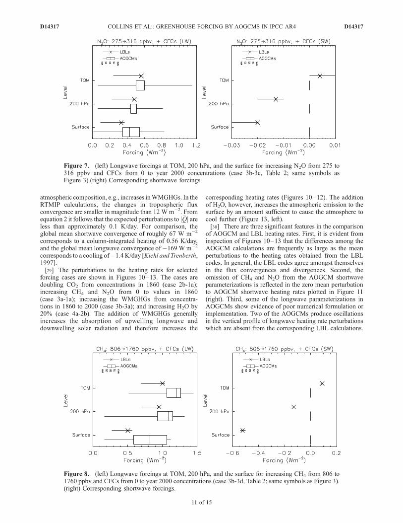
D14317

plotted in Figure 6. The forcings from increasing N2O andCFCs from concentrations at 1860 to 2000 are shown inFigure 7, and the corresponding forcings from increasingCH4 and CFCs are shown in Figure 8. The absorption byCFC-11 and CFC-12 occurs almost entirely between 5 and22.2 mm [e.g., Christidis et al., 1997] and therefore short-wave forcing by these compounds may be neglected. AsFigures 6–8 clearly show, all of the AOGCM codes in thisintercomparison omit the effects of CH4 and N2O onshortwave fluxes and forcings. While the omission ofN2O does not introduce a large absolute error in the forcings,recent increases in CH4 produce decreases of up to�0.5 W m�2 in the net shortwave fluxes at the surface inthe LBL calculations (S. Freidenreich, personal communi-cation, 2004). The AOGCMs also tend to overestimate thelongwave forcing at the surface by both N2O and CH4, andthese differences are statistically significant (Table 8). It isalso evident from Figures 7 and 8 that the ranges of LBLlongwave forcings for these cases are generally larger than

the corresponding ranges for the other cases. When CH4

and N2O are paired with CFC-11 and CFC-12, the spreadin LBL longwave forcings at each of the mandatory levelsis larger by at least 2 times than the corresponding range inthe LBL calculation with CH4 and N2O alone (Table 8). Inaddition, the spread in the LBL results for N2O combinedwith the CFCs is nearly identical to the spread for CH4

combined with the CFCs. These results indicate that thedivergence among LBL codes is related to the introductionof chlorofluorocarbons in the longwave calculations. Whilethe discrepancy has been traced to one of the LBL codes inthe intercomparison, the cause of the discrepancy has notbeen determined at this time. The authors and LBLdevelopers are continuing to investigate this issue. Theseresults imply that inaccuracies in the treatment of forcingby trace gases other than CO2 need further systematicanalysis.[27] The longwave forcing from increasing H2O is quite

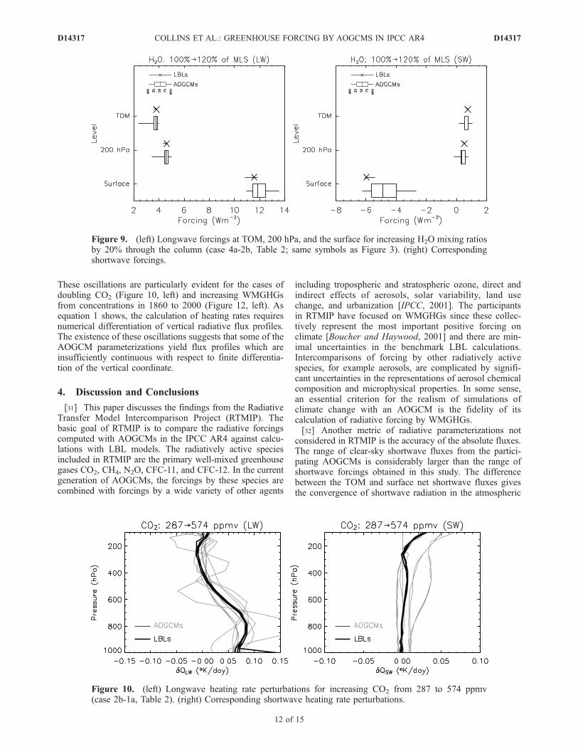
well simulated with the AOGCM codes (Figure 9). The

Figure 3. (left) Longwave forcings at TOM, 200 hPa, and the surface for increasing CO2 from 287 to369 ppmv (case 2a-1a, Table 2). AOGCM forcings are shown as box-and-whisker diagrams withpercentiles given in the legend. The minimum-to-maximum range and median are plotted for the LBLcodes. (right) Corresponding shortwave forcings.

Figure 4. (left) Longwave forcings at TOM, 200 hPa, and the surface for increasing CO2 from 287 to574 ppmv (case 2b-1a, Table 2; same symbols as Figure 3). (right) Corresponding shortwave forcings.


9 of 15

D14317

differences relative to the LBL calculations at the threestandard levels are not statistically significant. In the short-wave, the only significant difference between the AOGCMand LBL calculations occurs at the surface, where theAOGCMs tend to underestimate the magnitude of thereduction in insolation. The single sign error in the individ-ual AOGCM forcings relative to the LBL estimates occursin the shortwave forcing at 200 hPa. The error is evident inthe extension of the corresponding box-and-whisker dia-gram to negative values in Figure 9 (right). The fact that thesurface forcing from the H2O feedback is larger than thesurface forcing by the WMGHGs is consistent with earliermodeling studies of the interactions of the hydrologicalcycle and anthropogenic climate change [e.g., Ramanathan,1981].

3.2. Heating Rates From AOGCMs and LBL Models

[28] The perturbations to the heating rates by increases inWMGHGs and H2O are relatively small. The first law of

thermodynamics applied to just the radiative processes in avertically stratified atmosphere is:

r cp@T

@t¼ � @F

@zð1Þ

where r is the density of the atmosphere, cp is the specific heatof air at constant pressure, T is the atmospheric temperature,Fis a net radiative flux (positive upward), t is time, and z is thevertical coordinate. The radiative heating rates Q are equal to@T/@t with time expressed in days. Integrating this equationover the depth of a standard atmosphere and denoting themass-weighted heating rate by �Q gives

�Q ’ DF

120ð2Þ

with �Q expressed in units of K/day and the radiative fluxconvergence DF expressed inWm�2. This same relationshipapplies when �Q and DF are perturbed by changes in

Figure 5. (left) Longwave forcings at TOM, 200 hPa, and the surface for increasing WMGHGs fromyear 1860 to year 2000 concentrations (case 3b-3a, Table 2; same symbols as Figure 3). (right)Corresponding shortwave forcings.

Figure 6. (left) Longwave forcings at TOM, 200 hPa, and the surface for increasing CH4 from 0 to 806ppbv and N2O from 0 to 275 ppbv (case 3a-1a, Table 2; same symbols as Figure 3). (right) Correspondingshortwave forcings.


10 of 15

D14317

atmospheric composition, e.g., increases inWMGHGs. In theRTMIP calculations, the changes in tropospheric fluxconvergence are smaller in magnitude than 12 W m�2. Fromequation 2 it follows that the expected perturbations to j�Qj areless than approximately 0.1 K/day. For comparison, theglobal mean shortwave convergence of roughly 67 W m�2

corresponds to a column-integrated heating of 0.56 K/day,and the global mean longwave convergence of�169 Wm�2

corresponds to a cooling of�1.4K/day [Kiehl and Trenberth,1997].[29] The perturbations to the heating rates for selected

forcing cases are shown in Figures 10–13. The cases aredoubling CO2 from concentrations in 1860 (case 2b-1a);increasing CH4 and N2O from 0 to values in 1860(case 3a-1a); increasing the WMGHGs from concentra-tions in 1860 to 2000 (case 3b-3a); and increasing H2O by20% (case 4a-2b). The addition of WMGHGs generallyincreases the absorption of upwelling longwave anddownwelling solar radiation and therefore increases the

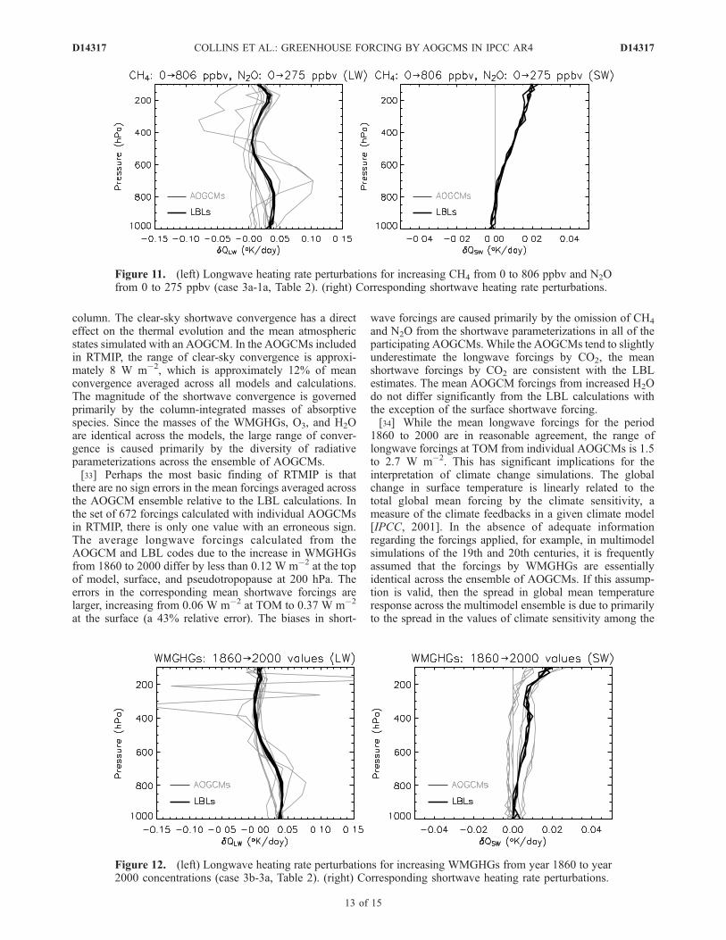
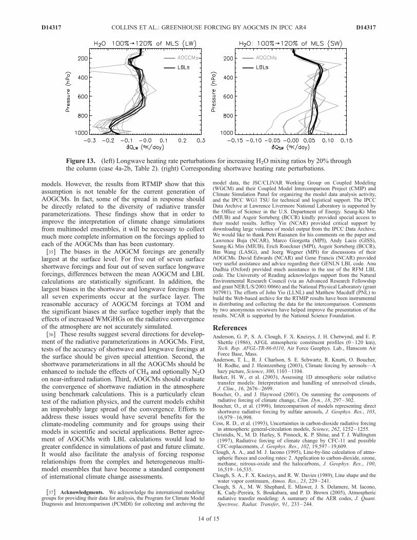
corresponding heating rates (Figures 10–12). The additionof H2O, however, increases the atmospheric emission to thesurface by an amount sufficient to cause the atmosphere tocool further (Figure 13, left).[30] There are three significant features in the comparison

of AOGCM and LBL heating rates. First, it is evident frominspection of Figures 10–13 that the differences among theAOGCM calculations are frequently as large as the meanperturbations to the heating rates obtained from the LBLcodes. In general, the LBL codes agree amongst themselvesin the flux convergences and divergences. Second, theomission of CH4 and N2O from the AOGCM shortwaveparameterizations is reflected in the zero mean perturbationto AOGCM shortwave heating rates plotted in Figure 11(right). Third, some of the longwave parameterizations inAOGCMs show evidence of poor numerical formulation orimplementation. Two of the AOGCMs produce oscillationsin the vertical profile of longwave heating rate perturbationswhich are absent from the corresponding LBL calculations.

Figure 7. (left) Longwave forcings at TOM, 200 hPa, and the surface for increasing N2O from 275 to316 ppbv and CFCs from 0 to year 2000 concentrations (case 3b-3c, Table 2; same symbols asFigure 3).(right) Corresponding shortwave forcings.

Figure 8. (left) Longwave forcings at TOM, 200 hPa, and the surface for increasing CH4 from 806 to1760 ppbv and CFCs from 0 to year 2000 concentrations (case 3b-3d, Table 2; same symbols as Figure 3).(right) Corresponding shortwave forcings.


11 of 15

D14317

These oscillations are particularly evident for the cases ofdoubling CO2 (Figure 10, left) and increasing WMGHGsfrom concentrations in 1860 to 2000 (Figure 12, left). Asequation 1 shows, the calculation of heating rates requiresnumerical differentiation of vertical radiative flux profiles.The existence of these oscillations suggests that some of theAOGCM parameterizations yield flux profiles which areinsufficiently continuous with respect to finite differentia-tion of the vertical coordinate.

4. Discussion and Conclusions

[31] This paper discusses the findings from the RadiativeTransfer Model Intercomparison Project (RTMIP). Thebasic goal of RTMIP is to compare the radiative forcingscomputed with AOGCMs in the IPCC AR4 against calcu-lations with LBL models. The radiatively active speciesincluded in RTMIP are the primary well-mixed greenhousegases CO2, CH4, N2O, CFC-11, and CFC-12. In the currentgeneration of AOGCMs, the forcings by these species arecombined with forcings by a wide variety of other agents

including tropospheric and stratospheric ozone, direct andindirect effects of aerosols, solar variability, land usechange, and urbanization [IPCC, 2001]. The participantsin RTMIP have focused on WMGHGs since these collec-tively represent the most important positive forcing onclimate [Boucher and Haywood, 2001] and there are min-imal uncertainties in the benchmark LBL calculations.Intercomparisons of forcing by other radiatively activespecies, for example aerosols, are complicated by signifi-cant uncertainties in the representations of aerosol chemicalcomposition and microphysical properties. In some sense,an essential criterion for the realism of simulations ofclimate change with an AOGCM is the fidelity of itscalculation of radiative forcing by WMGHGs.[32] Another metric of radiative parameterizations not

considered in RTMIP is the accuracy of the absolute fluxes.The range of clear-sky shortwave fluxes from the partici-pating AOGCMs is considerably larger than the range ofshortwave forcings obtained in this study. The differencebetween the TOM and surface net shortwave fluxes givesthe convergence of shortwave radiation in the atmospheric

Figure 9. (left) Longwave forcings at TOM, 200 hPa, and the surface for increasing H2O mixing ratiosby 20% through the column (case 4a-2b, Table 2; same symbols as Figure 3). (right) Correspondingshortwave forcings.

Figure 10. (left) Longwave heating rate perturbations for increasing CO2 from 287 to 574 ppmv(case 2b-1a, Table 2). (right) Corresponding shortwave heating rate perturbations.


12 of 15

D14317

column. The clear-sky shortwave convergence has a directeffect on the thermal evolution and the mean atmosphericstates simulated with an AOGCM. In the AOGCMs includedin RTMIP, the range of clear-sky convergence is approxi-mately 8 W m�2, which is approximately 12% of meanconvergence averaged across all models and calculations.The magnitude of the shortwave convergence is governedprimarily by the column-integrated masses of absorptivespecies. Since the masses of the WMGHGs, O3, and H2Oare identical across the models, the large range of conver-gence is caused primarily by the diversity of radiativeparameterizations across the ensemble of AOGCMs.[33] Perhaps the most basic finding of RTMIP is that

there are no sign errors in the mean forcings averaged acrossthe AOGCM ensemble relative to the LBL calculations. Inthe set of 672 forcings calculated with individual AOGCMsin RTMIP, there is only one value with an erroneous sign.The average longwave forcings calculated from theAOGCM and LBL codes due to the increase in WMGHGsfrom 1860 to 2000 differ by less than 0.12 W m�2 at the topof model, surface, and pseudotropopause at 200 hPa. Theerrors in the corresponding mean shortwave forcings arelarger, increasing from 0.06 W m�2 at TOM to 0.37 W m�2

at the surface (a 43% relative error). The biases in short-

wave forcings are caused primarily by the omission of CH4

and N2O from the shortwave parameterizations in all of theparticipating AOGCMs.While the AOGCMs tend to slightlyunderestimate the longwave forcings by CO2, the meanshortwave forcings by CO2 are consistent with the LBLestimates. The mean AOGCM forcings from increased H2Odo not differ significantly from the LBL calculations withthe exception of the surface shortwave forcing.[34] While the mean longwave forcings for the period

1860 to 2000 are in reasonable agreement, the range oflongwave forcings at TOM from individual AOGCMs is 1.5to 2.7 W m�2. This has significant implications for theinterpretation of climate change simulations. The globalchange in surface temperature is linearly related to thetotal global mean forcing by the climate sensitivity, ameasure of the climate feedbacks in a given climate model[IPCC, 2001]. In the absence of adequate informationregarding the forcings applied, for example, in multimodelsimulations of the 19th and 20th centuries, it is frequentlyassumed that the forcings by WMGHGs are essentiallyidentical across the ensemble of AOGCMs. If this assump-tion is valid, then the spread in global mean temperatureresponse across the multimodel ensemble is due to primarilyto the spread in the values of climate sensitivity among the

Figure 12. (left) Longwave heating rate perturbations for increasing WMGHGs from year 1860 to year2000 concentrations (case 3b-3a, Table 2). (right) Corresponding shortwave heating rate perturbations.

Figure 11. (left) Longwave heating rate perturbations for increasing CH4 from 0 to 806 ppbv and N2Ofrom 0 to 275 ppbv (case 3a-1a, Table 2). (right) Corresponding shortwave heating rate perturbations.


13 of 15

D14317

models. However, the results from RTMIP show that thisassumption is not tenable for the current generation ofAOGCMs. In fact, some of the spread in response shouldbe directly related to the diversity of radiative transferparameterizations. These findings show that in order toimprove the interpretation of climate change simulationsfrom multimodel ensembles, it will be necessary to collectmuch more complete information on the forcings applied toeach of the AOGCMs than has been customary.[35] The biases in the AOGCM forcings are generally

largest at the surface level. For five out of seven surfaceshortwave forcings and four out of seven surface longwaveforcings, differences between the mean AOGCM and LBLcalculations are statistically significant. In addition, thelargest biases in the shortwave and longwave forcings fromall seven experiments occur at the surface layer. Thereasonable accuracy of AOGCM forcings at TOM andthe significant biases at the surface together imply that theeffects of increased WMGHGs on the radiative convergenceof the atmosphere are not accurately simulated.[36] These results suggest several directions for develop-

ment of the radiative parameterizations in AOGCMs. First,tests of the accuracy of shortwave and longwave forcings atthe surface should be given special attention. Second, theshortwave parameterizations in all the AOGCMs should beenhanced to include the effects of CH4 and optionally N2Oon near-infrared radiation. Third, AOGCMs should evaluatethe convergence of shortwave radiation in the atmosphereusing benchmark calculations. This is a particularly cleantest of the radiation physics, and the current models exhibitan improbably large spread of the convergence. Efforts toaddress these issues would have several benefits for theclimate-modeling community and for groups using theirmodels in scientific and societal applications. Better agree-ment of AOGCMs with LBL calculations would lead togreater confidence in simulations of past and future climate.It would also facilitate the analysis of forcing responserelationships from the complex and heterogeneous multi-model ensembles that have become a standard componentof international climate change assessments.

[37] Acknowledgments. We acknowledge the international modelinggroups for providing their data for analysis, the Program for Climate ModelDiagnosis and Intercomparison (PCMDI) for collecting and archiving the

model data, the JSC/CLIVAR Working Group on Coupled Modeling(WGCM) and their Coupled Model Intercomparison Project (CMIP) andClimate Simulation Panel for organizing the model data analysis activity,and the IPCC WG1 TSU for technical and logistical support. The IPCCData Archive at Lawrence Livermore National Laboratory is supported bythe Office of Science in the U.S. Department of Energy. Seung-Ki Min(MIUB) and Asgeir Sorteberg (BCCR) kindly provided special access totheir model results. Jeffrey Yin (NCAR) provided critical support bydownloading large volumes of model output from the IPCC Data Archive.We would like to thank Petri Raisanen for his comments on the paper andLawrence Buja (NCAR), Marco Giorgetta (MPI), Andy Lacis (GISS),Seung-Ki Min (MIUB), Erich Roeckner (MPI), Asgeir Sorteberg (BCCR),Bin Wang (LASG), and Joerg Wegner (MPI) for discussions of theirAOGCMs. David Edwards (NCAR) and Gene Francis (NCAR) providedvery useful assistance and advice regarding their GENLN LBL code. AnuDudhia (Oxford) provided much assistance in the use of the RFM LBLcode. The University of Reading acknowledges support from the NaturalEnvironmental Research Council (via an Advanced Research Fellowshipand grant NER/L/S/2001/0066) and the National Physical Laboratory (grant307981). The efforts of John Yio (LLNL) and Matthew Macduff (PNL) tobuild the Web-based archive for the RTMIP results have been instrumentalin distributing and collecting the data for the intercomparison. Commentsby two anonymous reviewers have helped improve the presentation of theresults. NCAR is supported by the National Science Foundation.

ReferencesAnderson, G. P., S. A. Clough, F. X. Kneizys, J. H. Chetwynd, and E. P.Shettle (1986), AFGL atmospheric constituent profiles (0 –120 km),Tech. Rep. AFGL-TR-86-0110, Air Force Geophys. Lab., Hanscom AirForce Base, Mass.

Anderson, T. L., R. J. Charlson, S. E. Schwartz, R. Knutti, O. Boucher,H. Rodhe, and J. Heintzenberg (2003), Climate forcing by aerosols—Ahazy picture, Science, 300, 1103–1104.

Barker, H. W., et al. (2003), Assessing 1D atmospheric solar radiativetransfer models: Interpretation and handling of unresolved clouds,J. Clim., 16, 2676–2699.

Boucher, O., and J. Haywood (2001), On summing the components ofradiative forcing of climate change, Clim. Dyn., 18, 297–302.

Boucher, O., et al. (1998), Intercomparison of models representing directshortwave radiative forcing by sulfate aerosols, J. Geophys. Res., 103,16,979–16,998.

Cess, R. D., et al. (1993), Uncertainties in carbon-dioxide radiative forcingin atmospheric general-circulation models, Science, 262, 1252–1255.

Christidis, N., M. D. Hurley, S. Pinnock, K. P. Shine, and T. J. Wallington(1997), Radiative forcing of climate change by CFC-11 and possibleCFC-replacements, J. Geophys. Res., 102, 19,597–19,609.

Clough, A. A., and M. J. Iacono (1995), Line-by-line calculation of atmo-spheric fluxes and cooling rates: 2. Application to carbon-dioxide, ozone,methane, nitrous-oxide and the halocarbons, J. Geophys. Res., 100,16,519–16,535.

Clough, S. A., F. X. Kneizys, and R. W. Davies (1989), Line shape and thewater vapor continuum, Atmos. Res., 23, 229–241.

Clough, S. A., M. W. Shephard, E. Mlawer, J. S. Delamere, M. Iacono,K. Cady-Pereira, S. Boukabara, and P. D. Brown (2005), Atmosphericradiative transfer modeling: A summary of the AER codes, J. Quant.Spectrosc. Radiat. Transfer, 91, 233–244.

Figure 13. (left) Longwave heating rate perturbations for increasing H2O mixing ratios by 20% throughthe column (case 4a-2b, Table 2). (right) Corresponding shortwave heating rate perturbations.


14 of 15

D14317

Dudhia, A. (1997), RFM v3 software user’s manual, Tech. Rep. ESA PO-MA-OXF-GS-0003, Atmos., Oceanic, and Planet. Phys., Clarendon Lab.,Oxford, U. K.

Edwards, D. P. (1992), GENLN2: A general line-by-line atmospheric trans-mittance and radiance model, Tech. Rep. NCAR/TN-367+STR, 147 pp.,Natl. Cent. for Atmos. Res., Boulder, Colo.

Ellingson, R. G., and Y. Fouquart (1991), The intercomparison of radiationcodes in climate models—An overview, J. Geophys. Res., 96, 8925–8927.

Ellingson, R. G., S. J. Ellis, and S. B. Fels (1991), The intercomparison ofradiation codes used in climate models—Long-wave results, J. Geophys.Res., 96, 8929–8953.

Fels, S. B., J. D. Mahlman, M. D. Schwarzkopf, and R. W. Sinclair (1980),Stratospheric sensitivity to perturbations in ozone and carbon-dioxide—Radiative and dynamical response, J. Atmos. Sci., 37, 2265–2297.

Fels, S. B., J. T. Kiehl, A. A. Lacis, and M. D. Schwarzkopf (1991),Infrared cooling rate calculations in operational general circulation mod-els: Comparison with benchmark computations, J. Geophys. Res., 96,9105–9120.

Fouquart, Y., B. Bonnel, and V. Ramaswamy (1991), Intercomparing short-wave radiation codes for climate studies, J. Geophys. Res., 96, 8955–8968.

Goody, R. M., and Y. L. Yung, (1989) Atmospheric Radiation, 2nd ed., 519pp., Oxford Univ. Press, New York.

Halthore, R. N., et al. (2005), Intercomparison of shortwave radiative trans-fer codes and measurements, J. Geophys. Res., 110, D11206,doi:10.1029/2004JD005293.

Hansen, J., M. Sato, and R. Ruedy (1997), Radiative forcing and climateresponse, J. Geophys. Res., 102, 6831–6864.

Intergovernmental Panel on Climate Change (IPCC) (1995), ClimateChange, 1994: Radiative Forcing of Climate Change and an Evaluationof the IPCC IS92 Emission Scenarios, edited by J. T. Houghton et al., 339pp., Cambridge Univ. Press, New York.

Intergovernmental Panel on Climate Change (IPCC) (2001), ClimateChange 2001: The Scientific Basis, edited by J. T. Houghton et al.,944 pp., Cambridge Univ. Press, New York.

Kiehl, J. T., and K. E. Trenberth (1997), Earth’s annual global mean energybudget, Bull. Am. Meteorol. Soc., 78, 197–208.

Kratz, D. P., and F. G. Rose (1999), Accounting for molecular absorptionwithin the spectral range of the CERES window channel, J. Quant.Spectrosc. Radiat. Transfer, 61, 83–95.

Kratz, D. P., M. G. Mlynczak, C. J. Mertens, H. Brindley, L. L. Gordley,J. Martin-Torres, F. M. Miskolczi, and D. D. Turner (2005), An inter-comparison of far-infrared line-by-line radiative transfer models, J. Quant.Spectrosc. Radiat. Transfer, 90, 323–341.

Labs, D., and H. Neckel (1970), Transformation of the absolute solar radia-tion data into the ‘‘International practical temperature scale of 1968’’, Sol.Phys., 15, 79–87.

Liou, K.-N., (1992), Radiation and Cloud Processes in the Atmosphere,487 pp., Oxford Univ. Press, New York.

Manabe, S., and R. T. Wetherald (1975), The effects of doubling the CO2

concentration on the climate of a general circulation model, J. Atmos.Sci., 37, 3–15.

Myhre, G., and F. Stordal (1997), Role of spatial and temporal variations inthe computation of radiative forcing and GWP, J. Geophys. Res., 102,11,181–11,200.

Nakicenovic, N., and R. Swart (Eds.) (2000), Special Report of the Inter-governmental Panel on Climate Change on Emissions Scenarios, 570pp., Cambridge Univ. Press, New York.

Pawson, S., et al. (2000), The GCM-Reality Intercomparison Project forSPARC (GRIPS): Scientific issues and initial results, Bull. Am. Meteorol.Soc., 81, 781–796.

Ramanathan, V. (1981), The role of ocean-atmosphere interactions in theCO2 climate problem, J. Atmos. Sci., 38, 918–930.

Ramanathan, V., and R. E. Dickinson (1979), The role of stratosphericozone in the zonal and seasonal radiative energy balance of the Earth-troposphere system, J. Atmos. Sci., 36, 1084–1104.

Ramaswamy, V., and S. M. Freidenreich (1998), A high-spectral resolutionstudy of the near-infrared solar flux disposition in clear and overcastatmospheres, J. Geophys. Res., 103, 23,255–23,273.

Randall, D. A., (Ed.) (2000), General Circulation Model Development, Int.Geophys. Ser., vol. 70, 807 pp., Elsevier, New York.

Rothman, L. S., et al. (2003), The HITRAN molecular spectroscopic data-base: Edition of 2000 including updates of 2001, J. Quant. Spectrosc.Radiat. Transfer, 82, 5–42.

Schwarzkopf, M. D., and S. B. Fels (1985), Improvements to the algorithmfor computing CO2 transmissivities and cooling rates, J. Geophys. Res.,90, 10,541–10,550.

Shine, K. P., B. P. Briegleb, A. S. Grossman, D. Hauglustaine, H. Mao,V. Ramaswamy, M. D. Schwarzkopf, R. van Dorland, and W. C. Wang(1995), Radiative forcing due to changes in ozone: A comparison ofdifferent codes, in Atmospheric Ozone as a Climate Gas: General Circula-tion Model Simulations, NATO ASI Ser., Ser. I, vol. 32, edited by W. C.Wang and I. S. A. Isaksen, pp. 375–396, Springer, New York.

Stamnes, K., S. C. Tsay, W. Wiscombe, and K. Jayaweera (1988), Anumerically stable algorithm for discrete-ordinate-method radiativetransfer in multiple scattering and emitting layered media, Appl. Opt.,27, 2502–2509.

Tipping, R. H., and Q. Ma (1995), Theory of the water-vapor continuumand validations, Atmos. Res., 36, 69–94.

Tjemkes, S. A., et al. (2003), The ISSWG line-by-line inter-comparisonexperiment, J. Quant. Spectrosc. Radiat. Transfer, 77, 433–453.

Trenberth, K. E., (Ed.) (1992), Climate System Modeling, 788 pp.,Cambridge Univ. Press, New York.

Tukey, J. W. (1977), Box-and-whisker plots, in Exploratory Data Analysis,chap. 2C, pp. 39–43, Addison-Wesley, Reading, Mass.

Voigt, S., J. Orphal, D. Bogumil, and J. P. Burrows (2001), The temperaturedependence (203–293 K) of the absorption cross sections of O3 in the230 – 850 nm region measured by Fourier-transform spectroscopy,J. Photochem. Photobiol. A, 143, 1–9.

Zhong, W. Y., J. D. Haigh, D. Belmiloud, R. Schermaul, and J. Tennyson(2001), The impact of new water vapour spectral line parameters on thecalculation of atmospheric absorption, Q. J. R. Meteorol. Soc., 127,1615–1626.

��S. E. B. Casanova and L. K. Gohar, Department of Meteorology,

University of Reading, Earley Gate, P.O. Box 243, Reading RG6 6BB, UK.([email protected]; [email protected])W. D. Collins, Climate and Global Dynamics Division, National Center

for Atmospheric Research, P.O. Box 3000, Boulder, CO 80307, USA.([email protected])J.-L. Dufresne and M.-P. Lefebvre, Laboratoire de Meteorologie

Dynamique (LMD/IPSL), Tour 45–55, 3eme, Jussieu, CNRS/UPMC,Boite 99, F-75252 Paris Cedex 05, France. ([email protected]; [email protected])D. W. Fillmore, LSCE-Orme, Bat. 701, Orme des Merisiers, F-91191 Gif-

sur-Yvette, France. ([email protected])P. M. D. Forster, School of Earth and Environment, University of Leeds,

Leeds LS2 9JT, UK. ([email protected])Q. Fu, Department of Atmospheric Sciences, University of Washington,

408 ATG Building, P.O. Box 351640, Seattle, WA 98195, USA.([email protected])V. Y. Galin, Institute of Numerical Mathematics, Academy of Sciences, 8

Gubkina Street, Moscow 117333, Russia. ([email protected])W. J. Ingram, Department of Physics, Clarendon Laboratory, Parks Road,

Oxford OX1 3PU, UK. ([email protected])D. P. Kratz, Climate Science Branch, NASA Langley Research Center,

MS 420, 21 Langley Boulevard, Hampton, VA 23681, USA. ([email protected])J. Li, Canadian Centre for Climate Modeling and Analysis, University of

Victoria, P.O. Box 1700, STN CSC, Victoria, BC, Canada V8W 2Y2.([email protected])P. Marquet, Meteo-France, CNRM, 42 avenue G. Coriolis, F-31057

Toulouse Cedex 01, France. ([email protected])V. Oinas, NASA Goddard Institute for Space Studies, 2880 Broadway,

New York, NY 10025, USA. ([email protected])R. W. Portmann, Aeronomy Laboratory, NOAA, 325 Broadway, Boulder,

CO 80305, USA. ([email protected])V. Ramaswamy and M. D. Schwarzkopf, Geophysical Fluid Dynamics

Laboratory, 201 Forrestal Road, Princeton,NJ 08542,USA. ([email protected]; [email protected])Y. Sun, National Climate Center, CMA, Laboratory for Climate Change,

46 South Zhongguancun Avenue, Beijing 100081, China. ([email protected])Y. Tsushima, Frontier Research Center for Global Change, Japan Agency

for Marine-Earth Science and Technology, 3173-25 Showa-machi,Kanazawa-ku, Yokohama 236-0001, Japan. ([email protected])T. Uchiyama, Meteorological Research Institute, 1-1 Nagamine,

Tsukuba-shi, Ibaraki-ken 305–0052, Japan. ([email protected])W. Y. Zhong, Space and Atmospheric Physics Group, Physics

Department, Imperial College, Prince Consort Road, London SW7 2BW,UK. ([email protected])


15 of 15

D14317

Documents

Radiative forcing by well-mixed greenhouse gases