Radiation-induced refraction artefacts in the optical CT readout of polymer gel dosimeters

Warren G Campbell *1, Andrew Jirasek 1, Derek M Wells2, (1) University of Victoria, Victoria, BC (2) British Columbia Cancer Agency, Vancouver Island Centre, Victoria, BC Introduction As radiation therapy treatments become more complex, their verification will demand a more thorough set of dosimetry tools. One desirable dosimetry tool is the fully 3D, deformable, tissue-equivalent polymer gel dosimeter (PGD). In a PGD, monomers are spatially fixed in a gelatin structure and polymerize when exposed to ionizing radiation, increasing their opacity [1]. The relationship between optical density (OD) and absorbed dose can be established via appropriate dose calibration. In order to evaluate the 3D dose information that a PGD records, one must accurately measure its resultant polymer distribution. This distribution can be measured using optical computed tomography (CT). Analogous to x-ray CT, optical CT uses a beam of visible light to measure opacity projections of the PGD from multiple angles to reconstruct a map of its OD values [2]. However, the use of visible light introduces unique issues related to refraction. For instance, optical CT scanners typically require a matching bath—a bath of liquid with refractive index (RI) equal to that of the dosimeter. A matching bath ensures that rays of the optical beam maintain a linear trajectory as they encounter, traverse, and exit the PGD. In their pioneering 1996 work that established the OD-dose relationship of polymer gels, Maryañski et al also observed a slight increase in RI with dose. Over a range of 0–14 Gy, they saw an increase in refractive index of ~0.6% [1]. At that time, they predicted that such a small increase would not be significant enough to cause distortion errors in scans. Since then, one work by Oldham & Kim in 2004 attempted to observe any geometrical distortion that might be caused by this RI-dose relationship [3]. They observed no such radiation-induced distortion in their results. Apart from these two works, radiation-induced RI changes in PGDs have widely been assumed to be insignificant. The work here reveals the impact of radiation-induced refractive index changes in polymer gel dosimeters. Using a prototype fan-beam optical CT scanner [4], we identify optical CT refraction artefacts that are directly caused by radiation-induced RI changes. Investigative scans are used to demonstrate rayline errors occurring within and out of the plane of the fan-beam. Finally, we developed a sinogram space filtering technique that greatly reduces the magnitude of these errors. Methods Gel Dosimeters – Manufacture, Planning, & Irradiation Polymer gel dosimeters (see Fig. 1a) were produced by filling 1 L cylindrical flasks (Modus Medical Devices Inc.; London, ON) with a preparation of a normoxic polymer gel recipe (w/w%): 91.8% deionized water, 4.0% gelatin, 2.0% acrylamide, 2.0% N,N’-methylenebisacrylamide, and 9 mM tetrakis (hydroxymethyl) phosphonium chloride (all chemicals from Sigma-Aldrich; Oakville, ON). Gels were prepared as described in a previous work [4]. X-ray CT scans were performed for treatment planning purposes on a separate, unirradiated dosimeter using a General Electric HiSpeed FX/i single-slice CT scanner (GE Medical Systems; Milwaukee, WI). Treatment planning was performed using the Eclipse treatment planning system (TPS) (AAA v11.0.31, Varian Medical Systems; Palo Alto, CA). A TrueBeam linear accelerator (Varian) was used to deliver a cross-beam irradiation pattern featuring two, 3x3 cm2, 6 MV photon beams, 90° apart from one another, one contributing double the dose of the other. Using this relative weighting, the maximum dose in the central region of the distribution was 8 Gy. Optical CT and Investigative Scanning Optical scans of PGDs were performed using the latest version of a prototype fan-beam optical CT scanner (see Fig. 1b) [4]. Pre-irradiation and post-irradiation scans were acquired to provide transmission data for the PGD. A 5 cm axial range of the dosimeter was scanned to fully examine the dose distribution. Over that range, 50 slices were scanned using 720 projections over a full 360° rotation. A linear relationship between opacity and absorbed dose was assumed [1], so a single constant was used to convert all OD reconstructions into measured dose distributions. Investigative scans were performed using the same scan parameters described above, but with modifications to the scanner setup. Two types of investigative scans were used. The first type places a line-pair

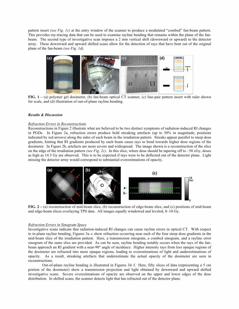
pattern insert (see Fig. 1c) at the entry window of the scanner to produce a modulated “combed” fan-beam pattern. This provides ray-tracing data that can be used to examine rayline bending that remains within the plane of the fan-beam. The second type of investigative scan imposes a 2 mm vertical shift (downward or upward) to the detector array. These downward and upward shifted scans allow for the detection of rays that have bent out of the original plane of the fan-beam (see Fig. 1d).

FIG. 1 – (a) polymer gel dosimeter, (b) fan-beam optical CT scanner, (c) line-pair pattern insert with ruler shown for scale, and (d) illustration of out-of-plane rayline bending. Results & Discussion Refraction Errors in Reconstructions Reconstructions in Figure 2 illustrate what are believed to be two distinct symptoms of radiation-induced RI changes in PGDs. In Figure 2a, refraction errors produce bold streaking artefacts (up to 50% in magnitude, positions indicated by red arrows) along the sides of each beam in the irradiation pattern. Streaks appear parallel to steep dose gradients, hinting that RI gradients produced by each beam cause rays to bend towards higher dose regions of the dosimeter. In Figure 2b, artefacts are more severe and widespread. The image shown is a reconstruction of the slice on the edge of the irradiation pattern (see Fig. 2c). In this slice, where dose should be tapering off to ~50 cGy, doses as high as 14.5 Gy are observed. This is to be expected if rays were to be deflected out of the detector plane. Light missing the detector array would correspond to substantial overestimations of opacity.

FIG. 2 – (a) reconstruction of mid-beam slice, (b) reconstruction of edge-beam slice, and (c) positions of mid-beam and edge-beam slices overlaying TPS data. All images equally windowed and leveled, 0–10 Gy. Refraction Errors in Sinogram Space Investigative scans indicate that radiation-induced RI changes can cause rayline errors in optical CT. With respect to in-plane rayline bending, Figures 3a–c show refraction occurring near each of the four steep dose gradients in the mid-beam slice of the irradiation pattern. Here, a transmission sinogram, a combed sinogram, and a rayline error sinogram of the same slice are provided. As can be seen, rayline bending notably occurs when the rays of the fan-beam approach an RI gradient with a near-90° angle of incidence. Higher intensity rays from less opaque regions of the dosimeter are refracted into more opaque regions, leading to overestimations of light and underestimations of opacity. As a result, streaking artefacts that underestimate the actual opacity of the dosimeter are seen in reconstructions. Out-of-plane rayline bending is illustrated in Figures 3d–f. Here, fifty slices of data (representing a 5 cm portion of the dosimeter) show a transmission projection and light obtained by downward and upward shifted investigative scans. Severe overestimations of opacity are observed on the upper and lower edges of the dose distribution. In shifted scans, the scanner detects light that has refracted out of the detector plane.

FIG. 3 – In-plane rayline errors: (a) transmission sinogram, (b) ray-tracing sinogram, and (c) rayline error sinogram of mid-beam slice; positions of all zoomed insets indicated by dashed box in (a). Out-of-plane rayline errors: (d) 2D transmission projection, (e) downward-shift scan data, and (f) upward-shift scan data of all 50 slices at a single projection angle. Sinogram Filtering An iterative Savitzky-Golay (ISG) filtering routine was developed to address refraction artefacts in sinogram space. The method is similar to another routine that is used to remove structured noise from x-ray CT reconstructions of PGDs [5]. The method developed here specifically targets structured errors in sinogram space by individually filtering each 2D projection (50 slices high, 320 detector elements wide) in the transmission sinogram (see Fig. 4). Outlier data are selectively replaced by filter results in each iteration. For comparison, projections were also filtered using an adaptive mean (AM) filter.

FIG. 4 – Effects of ISG filtering in sinogram space: (a) transmission sinogram, (b) absolute relative difference sinogram (i.e. |Raw – ISG|/ISG), (c) 2D transmission projection, and (d) absolute relative difference projection. Corrected Reconstructions Optical CT reconstructions and profile comparisons are illustrated in Figure 5. Comparisons include: i) treatment planning system data, ii) unfiltered data, iii) AM filtered data, and iv) ISG filtered data. As can be seen in Figure 5, the ISG and AM filtering routines were both able to remove a considerable amount of noise seen in unfiltered reconstructions. However, AM filtering is less capable than the ISG filtering routine in addressing the well-structured artefacts related to radiation-induced RI changes. The distinct streaking artefacts associated with in-plane rayline are effectively removed by the ISG routine. Although the much more severe artefacts associated with out-of-plane rayline errors were not fully removed by the ISG routine, the magnitude of these artefacts is greatly reduced. Additionally, the ISG routine addresses two unrelated artefacts that previously needed to be manually

removed from sinogram space—ring artefacts caused by data corruption in certain detector elements of the detector array, and streaking artefacts caused by a pair of vertical seams on the side of the flask that houses the dosimeter [4]. Unfortunately, due to its aggressive nature, the ISG routine also comes with its own limitations (e.g. edge degradation, potential loss of spatial resolution).

FIG. 5 – Reconstruction results: treatment planning system (TPS), unfiltered (Raw), adaptive mean filtered (AM), and iterative Savitzky-Golay filtered (ISG). Dashed lines overlaying TPS data indicate the positions of the three planes shown, which also correspond to the profile comparisons and difference profiles shown in (a) – (c). All images equally windowed and leveled, 0–10 Gy. Conclusions We have introduced a new category of imaging artefacts that can affect the optical CT readout of polymer gel dosimeters. Investigative scans were able to show that these artefacts are caused by radiation-induced RI changes. We were able to demonstrate rayline bending occurring parallel and perpendicular to the plane of the optical CT scanner’s fan-beam. Image reconstructions illustrated the symptoms of each type of rayline error. A filtering method to address these errors was developed and its effects shown. These findings provide useful insight for those intending to evaluate polymer gel dosimeters using optical CT. Additionally, these results provide recognizable signs to indicate that a given 3D dosimeter is exhibiting radiation-induced RI changes. Future investigations could examine the prevalence of these types of errors in more clinically relevant dose distributions and in other optical CT scanner geometries. Also, the PGD recipe might be altered to prevent radiation-induced RI changes. References [1] MJ Maryañski, YZ Zastavker, and JC Gore, Phys. Med. Biol. 41, 2705–2717 (1996). [2] JC Gore, M Ranade, MJ Maryañski, and RJ Schulz, Phys. Med. Biol. 41, 2695–2704 (1996). [3] M Oldham and L Kim, Med. Phys. 31, 1093–1104 (2004). [4] WG Campbell, DA Rudko, NA Braam, DM Wells, and A Jirasek, Med. Phys. 40, 061712 (2013). [5] A Jirasek, J Carrick, and M Hilts, Phys. Med. Biol. 57, 3137–3153 (2012).

A Nested Neutron Spectrometer to Measure Neutron Spectra in Radiotherapy

R Maglieri*1

, A Licea2, J Seuntjens

1, J Kildea

1,

(1) Medical Physics Unit, McGill University, Montreal, Qc (2) Canadian Nuclear Safety Commission CNSC,

Ottawa, Ontario

Introduction

During high-energy radiotherapy treatments, neutrons are produced in the head of the linac through photonuclear

interactions. This has been a concern for many years as photoneutrons contribute to the accepted, yet unwanted, out-

of-field doses that pose an iatrogenic risk to patients and an occupational risk to personnel. However, with the

advent of modern treatment planning dose calculation algorithms and IMRT, there is potential for a decrease in

neutron production through the use of un-flattened treatment beams. This motivates a quantification of the benefit of

flattening filter free beams in terms of neutron production.

Traditional in-room neutron measurements are difficult and time-consuming and are carried out using Bonner

spheres with activation foils and TLDs. Recently, a new neutron spectrometer, the Nested Neutron Spectrometer

(NNS) by Detec (Dubeau et al.), has appeared on the market. The NNS is uniquely designed for easy handling and is

more practical than the traditional Bonner spheres. It can be operated in current mode (not unlike an ion chamber)

and can be used to detect neutrons in high dose-rate environments.

The goal of this work is to evaluate the feasibility of using the NNS to measure neutrons in high dose-rate

environments such as radiotherapy treatment rooms. Energy spectra and equivalent doses measured using the NNS

are compared to Monte Carlo generated spectra and bubble detector measurements.

Methods

To determine the feasibility of using the NNS in radiotherapy, the equivalent dose at various points in the bunker is

compared to that of bubble detectors. Additionally, Monte Carlo simulations are used to evaluate the energy and

relative intensity of the thermal and fast neutron peaks of the neutron spectrum.

Measurements

All measurements were carried out in the bunker of a Varian Clinac 21EX linac at

our centre. The gantry and collimator were positioned at 0o and the linac was

operated in 18 MV mode at 600 MU/min with the jaws closed. The measurement

locations, as shown in Fig 1, were: 40 cm and 140 cm from the isocenter, at the

maze-room junction and in the maze. The point of measurement was kept at the

height of the isocenter in all cases.

Neutron spectra were measured

using the NNS (shown in Fig

2). The NNS comprises seven

high density polyethylene

(HDPE) moderators and a

central Helium-3 detector. The charge in the He-3 detector was

collected using a Keithley 6517A electrometer. Measurements

lasted one minute each (600 MU at 600 MU/min). Once the

charge was collected, it was converted to a count rate using a

calibration coefficient, 7 fA/cps, provided by the manufacturer.

Typical raw data collected from the NNS are shown in Fig 3.

Finally, the measurements were unfolded into 52 energy bins

using a custom developed maximum-likelihood expectation-

maximization (MLEM) algorithm.

FIGURE 2) The Nested Neutron Spectrometer. On left:

Helium-3 detector and its holder. On right: each

successive shell is added to the He-3 detector in order to sample a different part of the spectrum

FIGURE 1) Measurement locations

inside the Varian Clinac 21EX bunker

Bubble detectors (BTI, Chalk River) were used to measure the equivalent doses at the three farthest locations from

the linac head in Fig 1. Two types of bubble detectors were used: PND, sensitive to fast neutrons and BDT, sensitive

to thermal neutrons. The sum of their dose equivalents provides an estimate for the equivalent dose integrated across

the whole spectrum. The bubble detectors were irradiated for different amounts of MU based on their location as

shown in Table 1. The total MU in the maze was greater for the PND in order to compensate for the low number of

fast neutrons present in this region.

Position 40 cm 140 cm Maze-Room

Junction Maze

BDT (MU) - 5 20 60

PND (MU) - 5 20 340

Simulations

The neutron spectra were simulated using MCNP. Full linac head geometry was modeled using the published

geometry from Kase et al. 1998. The model is that of a Varian 2300C/D, however the beam line components were

updated in this work to reflect those in the Varian Monte Carlo Data Package. 5×108 electrons were used as starting

particles and the neutron production was scored in a phase space surrounding the linac. It was further propagated

into a fully described geometry of the bunker at our centre. The fluence spectrum is scored using a point detector (F5

Tally) with the same binning scheme as the NNS. Uncertainties for each bin were less than 3% in all cases.

Results and Discussion

The measured and simulated neutron spectra at each location are shown in Figs 4-7. For each measurement set, the

same a priori guess spectrum was used as input to the MLEM unfolding algorithm. The algorithm was halted when

the measurements and refolded data were within 1% of each other.

In each plot, the values are normalized to the maximum intensity peak of the spectrum. This allows us to perform a

qualitative comparison of the shape of the spectra. At 40 cm, the thermal neutron peak of the NNS is found to be

larger than that of the Monte Carlo. One possible explanation reason for this is that thermal neutrons arise from

multiple moderating events across the bunker. It is impossible to model every source of moderation (cabinets,

plastics) and thus the MC thermal peak is lower. At 140 cm, the thermal peak is also slightly larger and likely for the

FIGURE 3) Raw data obtained with the NNS using a calibration coefficient of, 7 fA/cps. Moderator is the number of moderator shells, where 0 is none and 7 is all

TABLE 1) Total Monitor Units at each of the measurement locations. The MU are larger in order to compensate for a low number of neutrons.

same reason as for the 40 cm case. Approaching the maze-room junction, the thermal neutron peak begins to

overtake the fast peak. As the measurement point is moved away from the linac head, most of the neutrons measured

are thermal and so the fast neutron peak is diminished. Finally, in the maze, the fast neutron peak is completely

suppressed in both the Monte Carlo and measurements. The moderating effect of the maze is clearly visible in both

the MC and NNS when moving from in the bunker to the maze.

Position 40 cm 140 cm Maze-Room

Junction Maze

Average Energy

MC (MeV) 0.48 0.36 0.17 0.03

Average Energy

NNS (MeV) 0.30 0.22 0.13 0.02

The average energies of the spectrum from the Monte Carlo and the NNS are shown in Table 2. These were

investigated to further evaluate the agreement between the Monte Carlo and the NNS. The differences range from

23-37%.

Shown in the Table 3 are the results of the bubble detector measurements. As expected, the dose equivalent was

largest closer to the linac and decreased as the point of measurement is moved further away. This is consistent with

the results of both the simulations and measurements. The NNS and bubble detector data agree within 10% at 140

cm and in the maze-room junction. In the maze itself, the percent difference is 50 %. For measurements at the maze-

room junction and in the maze, there is a statistical uncertainty of approximately 30-60% (95% confidence) due to a

low number of bubbles.

Position 40 cm 140 cm Maze-Room

Junction Maze

NNS

Equivalent Dose

(mSv/hr)

783.5 383.0 56.7 1.1

Bubble Detector

Equivalent Dose

(mSv/hr)

- 387.9 61.9 2.2

TABLE 2) Average energy of the Monte Carlo-simulated and NNS-measured spectra at each of the measurement locations.

TABLE 3) Equivalent doses measured with the NNS and bubble detectors. ICRP 74 conversion coefficients are used to convert fluence to dose.

FIGURE 4) Comparison of the measured and simulated neutron

spectra at 40 cm from the head of the linac .Data normalized to

maximum.

FIGURE 5) Comparison of the measured and simulated neutron spectra at 140 cm from the head of the linac. Data normalized to

maximum.

Conclusion

We have demonstrated the feasibility of using the Nested Neutron Spectrometer in high dose-rate radiotherapy

environments by comparing measurements from the NNS and bubble detectors at three different locations. The dose

equivalents agreed within uncertainty. Apart from some discrepancies at thermal energies, we also found reasonable

agreement between NNS-measured and Monte Carlo-simulated spectra at a number of locations within our

radiotherapy bunker.

Future work will compare absolute (un-normalized) Monte Carlo and NNS spectra and evaluate the manufacturer

provided calibration coefficient in order to resolve the observed discrepancies between the thermal peaks.

References

Kase, K. R., et al. "Neutron fluence and energy spectra around the Varian Clinac 2100C/2300C medical

accelerator." Health physics 74.1 (1998): 38-47.

Dubeau, J., et al. "A neutron spectrometer using nested moderators." Radiation protection dosimetry 150.2 (2012):

217-222.

Acknowledgments

R.M. acknowledges partial support by the CREATE Medical Physics Research Training Network grant of the

Natural Sciences and Engineering Research Council (Grant number: 432290) and the Canadian Nuclear Safety

Commission.

The author would like to gratefully acknowledge technical assistance and useful discussions with J. Dubeau and S.

Witharana, employees of Detec, Gatineau, Quebec.

FIGURE 6) Comparison of the measured and simulated neutron spectra at the maze-room junction .Data normalized to maximum.

FIGURE 7) Comparison of the measured and simulated neutron spectra in the maze .Data normalized to maximum.

Delta4 diode absolute dose response for large and small target volume IMRT QA

D Simard*1, V Thakur1 (1) Centre hospitalier de l’Université de Montréal, Montréal, Canada

Introduction With the increasing complexity of beam delivery coming with IMRT and VMAT techniques, the demand on patient plan specific QA has risen quickly. Several commercial solutions are available in the market to relieve the task, each with their advantages and drawbacks. At the Centre Hospitalier de l’Université de Montréal (CHUM), Delta4 (Scandidos, Uppsala, Sweden) has been used for about 5 years for routine delivery quality assurance (DQA) of helical Tomotherapy (Accuray, Sunnyvale, USA), RapidArc (Varian, Palo Alto, USA) and sliding window IMRT treatment plans. Its usefulness and accuracy have been shown [1, 2, 3]. However, limitations have also been observed for extreme clinical cases at the CHUM, for either large or small target volumes. The goal of this project was to quantify the over-response/under-response of the diodes for simple deliveries planned on extreme target sizes. Methods The Delta 4 phantom is cylindrical and consists of 2 diode planes arranged in an “X” shape squeezed by 4 quarter cylinder of PMMA. Scandidos provided us with a custom quarter that has a hole (perpendicular to the axial planes) and a plug to have the possibility to introduce an ionisation chamber (IC) close to the center of the phantom, 24mm up from the central diodes [Fig.1]. The CC13 IC (IBA, Schwarzenbruck, Germany) used in this study has been previously cross calibrated in a 6MV beam. This configuration gives the option to acquire simultaneous IC and diodes absolute dose measurements. IC has the advantage of being considered as a gold standard for absolute dose measurement for IMRT QA, due to their stability, linear response, small directional dependence and beam-quality response independence [4].

Fig1. Axial view of the custom Delta4 phantom for IC simultaneous measurement

A) Axial view B) Sagital view Eight plans for different target volumes [Fig.2] on this phantom were created using Tomotherapy TPS. Six plans were planned with the 25mm field width (FW) and two with 10mm FW. Targets were simple cylinders in the middle of the phantom, 20cm length with different diameter, 20cm, 15cm, 10cm, 5cm and 1cm. Another target was also used with the 25mm FW, 20cm length with varying size from 20cm to 5cm diameter. The 2 last plans were planned with the 10mm FW, one with the previous 20cm diameter cylinder and the last one with a small sphere of 1cm.

Fig2. Different targets used for planning (Blue,Brown,Cyan,red) and CC13 sensitive volume (green)

A) Axial view B) Sagital view Dose to the ionization chamber and the diodes on the Delta4 were measured simultaneously. However, we had to deliver 2 plans for the 1cm diameter targets because it was impossible to have both, diodes and IC, in the high dose region at the same time. Consequently, 2 plans have been optimized and delivered with translated targets centered on IC and on central diodes. For all the 8 plans, a sub volume of the target around the IC has been optimized to enhance homogeneity in this area.

For IC, measurements were compared with the average planned dose in its sensitive volume to verify the plan accuracy. To quantify the diodes absolute dose accuracy in the target, diodes dose measurements were compared with IC measurement. The first comparison was made with only diodes in the target close to the IC (∆close). The second comparison was made with all diodes inside the target (∆target). For both, we get a histogram of diode dose differences (Diode-IC) and the value reported corresponds to the histogram median. Results and Discussion For all 8 plans, IC measurements show a good agreement with planned dose (±2%). Diode measurements demonstrate a good agreement with IC for regular target size of 5 and 10cm (0 to1%). For larger targets, an over-response is observed for FW 25mm and 10mm (2 to 3%). A 2 to 3% over-response is more than enough for a plan to fail its gamma analysis of 3%/3mm tolerance. For small target of 1cm diameter, a major under-response is observed for FW 25mm and 10mm (-8 and -36%).

Tab.1 Diodes and IC difference for diodes in the target close to the IC (∆close) and for all

diodes inside the target (∆target) The over-response could to be due to the extra amount of scattered radiation and the opposite for under-response. When out of the primary beam, Delta4 diodes integrate signal of lower energy photons with a “low dose rate” as observed by the diodes. Helical delivery of Tomotherapy accentuates the “low dose rate effect” compared to conventional linac IMRT/VMAT plans for long targets. Helical Tomotherapy is probably the delivery technique for which the target voxels and so the diodes are outside the primary beam during the larger part of the beam on time. These diodes have been designed to have low dependencies on these 2 factors, but they can still be affected by them under certain conditions [5]. Although this scatter hypothesis still has to be proven, early testing demonstrates an over-response of 40% of the central diodes compare to IC when an open helical rotational beam is delivered 65mm away from the center of the phantom (beam edge to IC/diodes). This scatter measurement over-response goes to 20% when 25mm cm away. Similar scatter over-response results were obtained for conventional linac open rotational beam. Consequently, similar over-response/under-response is expected for large/small target volumes DQA on conventional linac (IMRT and VMAT). These results are in agreement with the real patient Delta4 DQA results at the CHUM. Medium target volume sizes DQAs typically have excellent gamma results and good dose agreements in the target (most of DQAs at the CHUM). DQA for large/small targets usually show an over-response/under-response compared to the planned dose. However, a recalculation and an extra delivery on a different phantom with IC often indicate a good agreement with planned dose. However, it’s much more complex to get clear results on real DQAs due to the complexity of the plans and the possible inhomogeneous dose in the IC volume. This custom PMMA Delta4 quarter will allow us to investigate more accurately the over-response/under-response of delta4 diodes on real DQAs. Conclusions Over-response and under-response of Delta4 diodes for Tomotherapy plans have been observed for large and small target size respectively, both in clinic and on artificial simple targets. The reason for this still has to be determined. This issue can certainly explain some gamma test fails of DQAs in the clinic. The next step in the process is to document this over-response and under-response for patient DQAs and to investigate this effect for IMRT and VMAT delivery. References [1] Geurts, M., Gonzalez, J., & Serrano-Ojeda, P. (2009). Longitudinal study using a diode phantom for helical tomotherapy IMRT QA. Medical physics, 36(11), 4977-4983. [2] Natali, M., Capomolla, C., Russo, D., Pastore, G., Cavalera, E., Leone, A., ... & Santantonio, M. (2013, July). Dosimetric verification of vmat dose distribution with DELTA4 Phantom. In 3rd Workshop-Plasmi, Sorgenti, Biofisica ed Applicazioni (pp. 80-83). [3] Bedford, J. L., Lee, Y. K., Wai, P., South, C. P., & Warrington, A. P. (2009). Evaluation of the Delta4 phantom for IMRT and VMAT verification. Physics in medicine and biology, 54(9), N167. [4] Low, D. A., Moran, J. M., Dempsey, J. F., Dong, L., & Oldham, M. (2011). Dosimetry tools and techniques for IMRT. Medical physics, 38(3), 1313-1338. [5] Bucciolini, M., Buonamici, F. B., Mazzocchi, S., De Angelis, C., Onori, S., & Cirrone, G. A. P. (2003). Diamond detector versus silicon diode and ion chamber in photon beams of different energy and field size. Medical physics,30(8), 2149-2154.

Radiation out-of-field dose in the treatment of pediatric central nervous system

malignancies

P J Taddei *1

, J Tannous1, R Nabha

1, J A Feghali

1, Z Ayoub

1, W Jalbout

1, B Youssef

1

*indicates presenting author

(1) Department of Radiation Oncology, American University of Beirut Medical Center, Beirut, Lebanon

Introduction

In radiotherapy, normal tissues receive radiation dose that can cause detrimental or even fatal late effects. These late

effects can manifest many months, years, or decades after treatment. Quantifying the probability of these late

effects is especially important for children who have good long-term prognoses because, in general, of the higher

sensitivity of their tissues and their smaller bodies and therefore closer proximity of their organs to the treatment

field than those of adults. These stray radiation exposures have no known benefit and result from radiation being

leaked from the treatment unit or scattered within the patient.

Children with cancer of the central nervous system (CNS) often receive radiotherapy as part of their treatment.

Depending on the type of tumor, their treatment plan may call for localized radiotherapy that targets a particular

treatment volume or regional radiotherapy (e.g., craniospinal irradiation) that targets the treatment volume and

subclinical disease.

Three-dimensional treatment planning system (TPS) computer algorithms are designed to calculate the absorbed

dose within the treatment fields with accuracy, but rarely calculate the dose that is deposited outside of the treatment

field with accuracy. In order to predict the risks of late effects, for example a radiation-induced second malignant

neoplasm, the out-of-field dose must be determined more accurately than what is possible with most commercial

TPSs.

The purpose of this study was to measure the out-of-field dose for a localized brain tumor treatment and develop an

analytical model for the absorbed dose versus distance from the field edge. These data were then coupled with those

of a previous study in which we developed a measurement-based analytical model for a regional craniospinal

irradiation radiotherapy treatment. Together, these models can be used to determine out-of-field dose and predict

the risk of late effects for pediatric patients receiving radiotherapy for CNS malignancies.

Methods

A three-dimensional conformal radiation therapy treatment was designed and delivered to an anthropomorphic

phantom (ATOM® Adult

Male 701, Computerized

Imaging Reference Systems,

Inc., Norfolk, Virginia) as if

it were a patient diagnosed

with low-grade astrocytoma.

Computed tomography

images were acquired for the

purposes of treatment

planning, patient setup, and

dose calculation and

transferred into our clinical

TPS (Prowess Panther

version 5.10, Prowess Inc.,

Concord, California) (figure

1). Field characteristics

designs were extracted from a

treatment plan of an actual

patient, a 12-year-old boy

diagnosed with anaplastic

ependymoma, in which the

Figure 1. Axial, sagittal, and coronal slices showing the dose distribution in

color wash and the 95% isodose line (red), 50% isodose line (light blue),

planning target volume (blue), and gross tumor volume (bright green).

tumor bed was targeted with a 7-field, 6-megavolt localized

radiation therapy. These fields were applied to the posterior

fossa region of the phantom. Absorbed dose was calculated

for the full treatment, with a weighting point placed in the

center of the target volume.

Thermoluminescent dosimeters (TLDs) composed of lithium

fluoride TLD-100 powder capsules (Quantaflux Radiological

Services, San Jose, California) were placed in 215 locations

throughout the phantom, mostly outside of the treatment

fields. TLDs were also placed in 34 locations on the surface

of the phantom, but these data were not used in this study.

Although the original treatment had a prescription of 50.4 Gy

to be delivered to the target volume in 1.8-Gy fractions,

because of the detection limitations of the TLDs, we scaled

the dose to 32.4 Gy to the weighting point, and delivered it in

a single fraction (figure 2) with a linear accelerator (Artiste,

Siemens Medical Solutions USA, Inc., Malvern,

Pennsylvania). A second measurement was made with a second set of TLDs, in which the same fields were

delivered except with the dose increased by a factor of 20. The purpose of this second measurement was to obtain

accurate absorbed dose measurements in the lowest-dose regions. For this reason, only TLDs locations with less

than 0.3 Gy were re-measured. These irradiated TLDs along with six background TLDs were sent to the Imaging

and Radiation Oncology Core (Houston, Texas) for analysis.

A contour was automatically created in the TPS for the composite field edge (i.e., 50% isodose line), and using in-

house codes, we calculated the distance from each TLD position to the field edge. A double-Gaussian equation for

out-of-field dose, D, versus distance from the field edge, r, that was used in the craniospinal irradiation study was

applied here also,

.

The parameters σ1, σ2, μ1, μ2, α1, and α2 were allowed to vary and were fit to the model by minimizing the root mean

square deviation, RMSD, between the doses calculated by the model and the measured doses

Unlike the previous study, in this

study the angle of the treatment

couch varied, which placed

TLDs located outside the 50%

isodose line within one or more

fields. For this reason, these

TLD locations and all TLDs

superior to the upper neck (i.e.,

just above the position of the

thyroid) were excluded from the

model fitting.

Results and Discussion

The absorbed dose measured

with each TLD that was used to

fit the double-Gaussian model

are shown in figure 3 along with

the resulting analytical model.

The plot is only shown to 80 cm

from the field edge because this

is a conservative maximum

2 2

1 2

2 21 22 21 2

2 2

1 22π 2π

r r

D e e

Figure 2. The TLD-loaded phantom placed in

the treatment position for one for the treatment

fields.

0

5

10

15

20

25

0 20 40 60 80

Do

se

(c

Gy/G

y)

Distance from field edge (cm)

TLD data

Model Fit

0

0.1

0.2

0.3

0.4

0.5

0 20 40 60 80

Figure 3. Absorbed dose at each TLD location per prescribed dose at the

weighting point (blue markers) along with the model fit to the data (red

line).

distance for pediatric CNS patients from the target volume to an organ that is of concern for radiation

carcinogenesis. The model followed the data very well out to about 50 cm from the field edge. However, from 50

cm to 80 cm, the model underestimated the actual data. The RMSD for these data was 2.85 cGy/Gy.

The model also poorly predicted the absorbed dose for locations in which the distance from the field edge was less

than 4 cm. This finding was contrary to our previous study for craniospinal irradiation. The reason for this new

result is that these locations within 4 cm of the composite field edge may be very close to one of the treatment fields

and may be affected by therapeutic radiation rather than scatter or leakage radiation. This was true even when we

attempted to remove these data points from consideration.

Based on the above observations, this analytic model may be very useful in the region between 4 cm and 50 cm.

The RMSD for the data in which 4 cm < r < 50

cm was 0.54 cGy/Gy. Within 4 cm from the

composite field edge, the dose calculated by the

TPS may be more accurate than the dose

calculated by this model. Between 50 cm to 80

cm from the composite field edge, the model

failed. Therefore, a new model should be

considered, for example with a third Gaussian or

linear term.

The model fit from this localized CNS

radiotherapy study is plotted along with the

model fit from the previous regional CNS

radiotherapy study in figure 4. Very close to the

field (r < 4 cm), the out-of-field dose estimated

by the model was higher for the localized CNS

radiotherapy than for the regional radiotherapy.

At moderate distances from the field (4 cm < r <

20 cm), the out-of-field dose estimated for

localized CNS radiotherapy was much lower

than that of regional CNS radiotherapy.

Conclusions

We developed a measurement-based analytical model for out-of-field absorbed dose versus distance from the field

edge for a localized brain treatment. This model may be applicable for points at distances from the field edge

between 4 cm and 50 cm, but for points beyond 50 cm, an improved model may be developed and applied. As a

result of this study, we now have a more definitive and accurate understanding of radiation absorbed dose received

by tissues in beyond the treatment field.

The model developed in this study for localized brain cancer radiotherapy, together with a model developed

previously for regional (craniospinal) radiotherapy for brain cancer, can be used for estimating out-of-field absorbed

dose in the treatment of pediatric CNS malignancies. However, more work is needed to improve accuracy of the

dose calculated very far away from the treatment field in localized brain cancer treatments.

Figure 4. Double-Gaussian analytical models fit to TLD-

measured data for a regional (craniospinal) irradiation and a

localized (three-dimensional conformal) irradiation for

cancer of the CNS.

0

5

10

15

20

25

30

35

40

0 5 10 15 20 25 30

Do

se

(c

Gy/G

y)

Distance from field edge (cm)

Regional Pediatric CNS Radiotherapy

Localized Pediatric CNS Radiotherapy

Megavoltage electron backscatter: EGSnrc results versus 21 experiments

E. S. M. Ali*,1,2

, W. Buchenberg1,3

, and D. W. O. Rogers1,

(1) Carleton University, Ottawa, Canada (2) The Ottawa Hospital Cancer Centre, Ottawa, Canada (3) University

Medical Center, Freiburg, Germany

Introduction

Electron backscatter is a stringent test for any Monte Carlo code that uses the condensed history technique to model

electron transport1. Establishing the accuracy of electron backscatter calculations at megavoltage energies is

important for many medical physics applications such as: (a) wall correction factors for parallel plate chambers in

clinical electron beams, where a significant component of the correction is from electron backscatter from the back

wall that is not water equivalent2,3

; (b) interface perturbations in electron treatments4, e.g., due to hip implants; (c)

beta emitters, e.g., Sr90

/Y90

, that are used for the treatment of superficial tumors5; and, (d) calculations for electron

beam shaping (e.g., applicators and cutouts)6. In this study, EGSnrc

1 backscatter calculations for megavoltage

electrons are performed and compared to the aggregate of experimental measurements in the literature. Two

quantities are investigated: the backscatter coefficient and the energy distribution of backscattered electrons. The

backscatter coefficient is the ratio of the number of backscattered electrons in the backward hemisphere to the

number of incident electrons, and it is typically expressed in per cent. The energy spectra are investigated for the

backscattered electrons in the backward hemisphere, and also at specific detector locations behind the target.

Methods

Experimental measurements: Data are compiled and analyzed for 21 experiments published between 1954 and 1993

for the energy range from 1 to 22 MeV. The targets are 25 single elements with atomic numbers from 3 to 92 and

they are fully stopping of the respective incident electron beams. The most commonly used detector is Faraday cup;

other detectors include ion chambers, silicon detectors, thermoluminescent detectors and calorimetry. Surface

electrons (< 50 eV) are suppressed (typically using a negatively biased grid) and they do not contribute to the

backscatter results. For a given electron energy and target element, the typical spread of the backscatter coefficient

among the 21 experiments is ~15%, which is of the order of the reported experimental uncertainties.

EGSnrc simulations: Calculations are performed assuming an ideal detector. The effects of a number of physics

processes and simulation parameters are investigated. For example, figure 1 demonstrates the importance of

modelling the relativistic electron spin. Figure 2 indicates that a larger electron energy cutoff (ECUT) introduces

systematic errors for low atomic number elements with high energy electrons, which is largely from the contribution

of lower energy secondary electrons, as seen in figure 3. The final calculations are done with accuracy in favor of

efficiency. The combined statistical and systematic uncertainty in the EGSnrc calculations is estimated to be 3%.

Results

Representative results for the backscatter coefficient are

shown in figures 4, 5 and 6. The overall agreement is within

2% in the absolute value of the backscatter coefficient (in per

cent), and within 11% of the individual backscatter values.

EGSnrc results are systematically on the higher end of the

spread of the experimental data. The experimental literature

indicates that the sources of systematic errors that reduce the

measured backscatter coefficient are more than those that

increase it. This could partially explain the trends observed in

the results. Representative results for the energy spectra are

shown in figures 7, 8 and 9. Reasonable agreement between

simulations and experiments is observed, and the variations

among different experiments are also obvious. At the lower

end of the energy spectra, EGSnrc is higher than some

experimental data. This could be due to reduced sensitivity of

the experiments to lower energy electrons (e.g., lower signal-

to-noise ratio, higher loss rate) and/or due to over-estimation

by EGSnrc for backscattered secondary electrons (cf. figure

3). The discrepancies close to the high end of the spectra are

likely related to experimental errors (e.g., energy spread of the

incident beam, as in figure 9).

Figure 1: Effect of modelling relativistic

electron spin on the calculated backscatter

coefficients. Spin effects are turned ON for

the final calculations.

Figure 3: Calculated energy distribution of

backscattered 1 MeV electrons. The

contribution of primary (i.e., incident) and

secondary electrons is shown.

Figure 2: Effect of the electron energy cutoff

(ECUT) on the accuracy of the calculated

backscatter coefficients, compared to the most

accurate results with a 1 keV electron kinetic

energy cutoff.

Figure 4: Comparison of EGSnrc calculations

against measured data from 21 experiments

for the variation of the backscatter coefficient

with the incident electron kinetic energy. Data

for other elements are comparable. The scale

of abscissa is logarithmic.

Figure 5: Same as figure 4, but for the

variation of the backscatter coefficient with

atomic number for 1 MeV incident electron

energy. Data for other incident electron

energies are comparable.

Conclusions

Overall good agreement is observed between EGSnrc calculations and experimental measurements of backscatter

coefficients and energy spectra for megavoltage electron beams. EGSnrc results for the backscatter coefficients are

systematically on the higher end of the spread of the experimental data. At the lower end of the energy spectra,

EGSnrc results are higher than some experimental data, but the quality of the experimental data precludes further

analysis. There is a need for high quality experimental data for the energy spectra of backscattered electrons.

References

[1] Kawrakow, Med. Phys. 27 485 – 498 (2000)

[2] Klevenhagen, Phys. Med. Biol. 36 1013 – 1018 (1991)

[3] Buckley and Rogers, Med. Phys. 33 1788 – 1796 (2006)

[4] Verhaegen, Phys. Med. Biol. 48 687 – 705 (2003)

[5] Buffa et al, Cancer Radiother. Radiopharma. 18 463 – 471 (2003)

[6] Chow and Grigorov, Med. Phys. 35 1241 – 1249 (2008)

Figure 8: Same as figure 7, but for electrons

backscattered at 102.5o relative to the

direction of incidence of the 1 MeV primary

electron beam.

Figure 9: Same as figure 7, but for electrons

backscattered at 120o relative to the direction

of incidence of the primary electron beam.

Data for the 15 and 24.8 MeV beams are

offset for clarity. Note the logarithmic scale

of the ordinate.

Figure 6: Same as figure 4, but for the variation

of the backscatter coefficient with the angle of

incidence of the 1.2 MeV electron beam.

Figure 7: An example of the comparison of

EGSnrc results against experimental data for

the energy distribution of 1 MeV electrons

backscattered in the backward hemisphere.

Commissioning of a 3D patient specific QA system for hypofractionated prostate treatments

R Rivest*1, S Venkataraman1, B McCurdy1,2

(1) CancerCare Manitoba (2) University of Manitoba

Introduction The complexities associated with the planning and delivery of advanced treatment techniques such as SRS, SBRT and VMAT pose additional challenges for ensuring quality radiation therapy treatments. Errors can occur during dose calculation, information transfer and treatment delivery. As such, it is common practice to QA individual treatment plans using either calculation or measurement based approaches. At our centre, patient specific QA of 6MV DMLC-IMRT and VMAT plans is performed using the COMPASS (v2.1, IBA-Dosimetry) system.1,2 The system consists of a 2D ion chamber array (MatriXXEvolution), an independent gantry angle sensor and associated software. The system requires a beam model that is developed and commissioned in the same manner as a beam model is commissioned in a standard treatment planning system. Hypofractionated prostate treatments3,4 at our centre are delivered with the 6MV-SRS beam on a Trilogy (Varian Medical Systems) linear accelerator in order to take advantage of its higher maximum dose rate compared to the standard 6MV beam (1000 MU/min vs 600 MU/min). Currently, a phantom based approach is used for QA of these plans as a 6MV-SRS beam model has yet to be generated in the COMPASS system. The objective of this work is to commission the 6MV-SRS beam model in COMPASS and validate its use for patient specific QA of hypofractionated prostate treatments. Methods The COMPASS software consists of two methods (calculation and reconstruction) for carrying out independent dose computation and comparison with the treatment planning system calculated dose distribution. In COMPASS calculations, the system generates a fluence using the imported plan and a commissioned beam model. A dual source (i.e. focal and extra-focal) photon head fluence model is assumed. The fluence is projected onto the patient CT dataset and dose is calculated using a collapsed cone convolution superposition algorithm. In COMPASS reconstructions, the plan is delivered to the MatriXXEvolution detector mounted in the gantry at a source to detector distance of 76.2 cm. The detector contains 1020 vented parallel plate ion chambers arranged in a 32 x 32 grid. Using a library of Monte Carlo generated detector response kernels, the commissioned beam model and the imported plan, detector response measurements are converted to a delivered fluence, which is then projected onto the 3D CT data and dose is calculated using the collapsed cone convolution superposition algorithm. The first step in commissioning of the 6MV-SRS beam model is the acquisition of measured beam data. Multiple ion chambers and diodes were used to characterize the radiation beam for small fields. Based on the analysis, a Pinpoint ion chamber (PTW Dosimetry) was used for output factor and percentage depth dose (PDD) measurements. Mellenberg-corrected Markus chamber measurements were used for the buildup region of PDDs. Crossplane profile measurements were done using SFD and PFD diodes (IBA Dosimetry). The data for various field sizes ranging from 1 cm x 1 cm to the maximum field size for the 6MV-SRS beam of 15 cm x 15 cm were imported into the COMPASS software. Similar to a planning system, the beam modeling process consists of adjusting model parameters such as the photon energy spectrum, electron contamination, off-axis softening, the width and weight of the two sources and MLC parameters until calculated beam data agrees with the measured data within an acceptable level of accuracy. As a starting point, the commissioned 6MV beam model was initially assumed. The photon energy spectrum and electron contamination parameters were adjusted based on PDDs while the other parameters that affect open field dose calculations were predominantly adjusted using the off-axis profiles. MLC parameters were adjusted based on comparisons with bar and strip patterns delivered to film.

Model validation was initially performed using open fields of various sizes. Both COMPASS calculations and reconstructions were compared to measured data. In addition, 10 prostate RapidArc plans were delivered to the Medtec phantom using our standard clinical method for patient specific QA of these patients. An EBT2 film and a single ion chamber were inserted into the phantom during irradiation. The ten plans were also delivered to the COMPASS system and both COMPASS calculations and reconstructions were performed on the phantom CT dataset. Reconstructed and computed doses at the ion chamber point and the film plane were compared with measurement. Gamma analysis, using a 3%/3mm criteria was performed when comparing COMPASS dose distributions and film measurements. The Medtec phantom as well as the setup of the COMPASS system for measurement are depicted in Figure 1.

Figure 1: Medtec phantom (left) and COMPASS system (right).

Results and Discussion The dose rate at a depth of 10 cm in a water phantom for a 10 cm x 10cm open field and an SSD of 100 cm, as determined by ion chamber measurement, TPS (Eclipse, Varian Medical Systems), COMPASS calculation and COMPASS reconstruction are 0.639 cGy/MU, 0.637 cGy/MU, 0.636 cGy/MU and 0.636 cGy/MU, respectively. Output factors for various field sizes are provided in Table 1. Off-axis profiles calculated by COMPASS for a 10 cm x 10 cm field are compared with measurement in Figure 2.

Table 1: Output factors for the 6MV-SRS beam

Field Size Measurement TPS COMPASS Reconstruction

COMPASS Calculation

3 cm x 3 cm 0.856 0.855 0.854 0.855 5 cm x 5 cm 0.910 0.908 0.913 0.910 15 cm x 15 cm 1.054 1.054 1.053 1.055

The mean (± standard deviation) difference between COMPASS reconstructed dose and ion chamber measurement in the Medtec phantom for the ten plans was 1.4 ± 1.0 %. The maximum discrepancy was 2.6%. Corresponding values for COMPASS calculation were 0.9 ± 0.9 % and 2.6 %, respectively. The gamma agreement index evaluated when comparing COMPASS to film was determined using both a 70% and a 20% dose threshold. Gamma agreement index values are listed in Table 2. In the phantom based approach that is currently used at our centre for patient specific QA of patients treated with the 6MV-SRS beam, tolerances for point dose measurements and gamma agreement index are 3% and 95%, respectively. Assuming these metrics are transferable to the present analysis, all COMPASS calculations and reconstructions at the ion chamber point have acceptable agreement with measurement. As for the gamma analysis, there are only two data points below the 95% gamma agreement index tolerance.

Table 2: Gamma agreement index comparing COMPASS to film

Dose Threshold Average Maximum Minimum 70 % 96.7 % 97.4 % 95.9 % COMPASS

Reconstruction 20 % 95.3 % 98.2 % 89.2 % 70 % 97.1 % 98.4 % 95.9 % COMPASS

Calculation 20 % 97.1 % 99.9 % 93.6 %

Figure 2: Comparison of measured and COMPASS calculated off-axis profiles for a 10 cm x 10 cm field at various depths.

Conclusions A 6MV-SRS beam model in COMPASS has been commissioned and validated by comparing COMPASS dose calculations and reconstructions to measured open field beam data. The COMPASS system was validated for use in the patient specific QA of hypofractionated prostate treatments delivered with the Varian 6MV-SRS beam. Conflict of Interest Statement A research contract was in place between CancerCare Manitoba and IBA Dosimetry during the time period in which this work was performed. References

1Boggula et al. Patient-specific 3D pretreatment and potential 3D online dose verification of Monte Carlo-calculated IMRT prostate treatment plans. Int J Radiat Oncol Biol Phys. 2010;81(4):1168-75. 2Boggula et al. Experimental validation of a commercial 3D dose verification system for intensity-modulated arc therapies. Phys Med Biol. 2010;55(19):5619-33. 3Wong et al. The case for hypofractionation of localized prostate cancer. Rev Urol. 2013;15(3):113-7. 4Cabrera and Lee. Hypofractionation for clinically localized prostate cancer. Semin Radiat Oncol. 2013;23(3):191-7.