R language Project report

PSTAT 174 Project report

Forecasting on global warming in the future 10 years

Tianyue Wang

Pstat 174

Section: Friday 10am

Abstract

Is it true that the whole world is experiencing a significant increase of global

temperature? If so, how fast is the temperature growing? Should we be worried about

global warming in 10 years? In this project, my goal is to solve these questions by

studying a time series measuring the evolution of global temperature, while trying to

fit in a model in order to give a prediction on the land-air temperature for the next ten

years using software R. After fitting in an ARIMA(2,1,2) model, I get a positive result

that the global land-surface temperature is decreasing slightly and steadily in the

future ten years, which indicates that we do not need to worry too much about global

temperature in a few years.

Key words: global warming, forecasting, time series plot, acf & pacf,

differencing, fit ARIMA models, AICc, diagnostic checking, etc.

I. Introduction

The data I choose for my project collects the temperature anomaly time series

during the time period from 1856 to 1997, which are derived from a global database

of corrected land and marine temperature data. The anomalies are based on

land-surface temperatures observed by CDIAC (Carbon Dioxide Information

Analysis Center) and have been used in various IPCC (Intergovernmental Panel On

Climate Change) reports. According to the data, the world has experienced the

warmest years since 1990, and the temperature of year 1997 reached the peak. The

reason I believe this project is important is that global warming is a serious matter to

our life. Analyzing this land-surface temperature data set is a great way to study

global warming, and predicting the future global temperature based on the data could

help prevent the future disasters in advance.

The main question of this project is should we be worried of global warming in

the future ten years. In order to solve this question, I used R to analyze the original

data and tried to fit in a model. First of all, I checked the trend and seasonality based

on the time series plot, ACF and PACF. Next, I used differencing at lag 1 in order to

to get a stationary time series. Thus, I estimated the parameters based on the ACF and

PACF of the differenced series. After suggesting eight possible models, I checked the

smallest AICc as well as their invertiblity and casuality, which eliminated to three

models as result. Though all of the three models passed the diagnostic checking, I

choose ARIMA(2,1,2) according to the principle of parsimony. Based on the model,

my forecasting turned out a positive result, which I suggest we should not be

worried about global warming in the future ten years since the prediction shows

a steady and slightly decrease.

II. Sections According to the following time series plot, it is not a stationary process since

there is an upward trend which shows a significant increase of the global land-air

temperature. The mean is -0.1580986 while the variance is 0.04747083. Also, there

is no obvious seasonality demonstrated in the plot. According to the graph, there are

about three significant sharp changes in approximately year 1880, 1918 and 1944.

Before the 1900s, there was a sudden increase of the temperature around year 1880,

which increased from approximately -0.4 to 0. However, the next year experienced an

obvious decrease approximately from 0 to -0.3. The second sharp change happened

around year 1918, which raised from -0.58 to -0.1, and then dropped to -0. 56. The

last one happened around year 1944, which increased from approximately -0.1 to 0.25

and then dropped to -0.2. Thus, according to the plot, the temperature reached its

highest point in year 1997 and reached its lowest point in approximately 1862 and

1908.

From the above Autocorrelation function plot (acf), the slow decay of ACF points

shows non-stationarity. In order to get a stationary series, I differenced the data at lag

1 first to remove the trend. Since there are negative values in the data set, it is easier

to use differencing than to use transformations like box-cox transformation or log

transformation, as these transformations requires adding process.

Parameter estimation

After differencing the time series at lag 1, the new times series plot appears to be

stationary. The mean appears to be 0.005602837, which is approximately 0. While the

variance decreased from 0.04747083 to 0.0146791. Also, the ACF shows no

seasonality. Since both the ACF plot and PACF plot tails off quickly, it is possible to

use ARIMA model here. According to the acf plot, the acf cuts off at lag 1 or lag 2,

which indicates that Q could be equal to 1 or 2. According to the PACF plot, it cuts

off at lag 1, 2, 3 or 36, which indicates that P could be 1, 2, 3 or 36. Since I

differenced once to remove the trend, d=1. This suggests the models could be:

ARIMA(1,1,1) ARIMA(1,1,2) ARIMA(2,1,1) ARIMA(2,1,2) ARIMA(3,1,1) ARIMA(3,1,2) ARIMA(36,1,1) ARIMA(36,1,2)

Fit the models

In order to find the best model, I fit these models and then checked their AICc in

order to find out the one with the smallest AICc. In result, ARIMA(2,1) has the

lowest AICc (-220.9312) while ARIMA(1,1), ARIMA(1,2), ARIMA(2,2),

ARIMA(3,1) and ARIMA(3,2) have similar AICc. The following are the formulas for

the models:

Model 1 ARIMA(2,1,1): lowest AICc; Model 2 ARIMA(1,1,1): second lowest AICc; Model 3 ARIMA(3,1,1) Model 4 ARIMA(1,1,2) Model 5 ARIMA(3,1,2) Model 6 ARIMA(2,1,2)

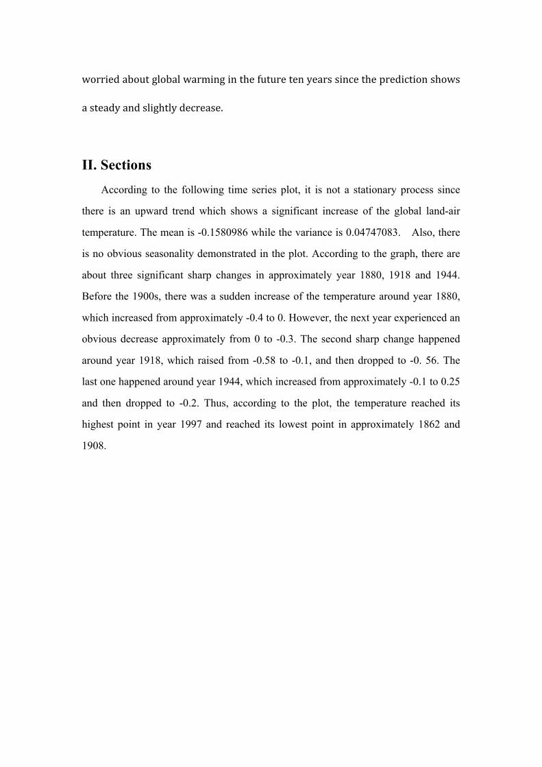
After fit in these models, I plot the roots of AR part to check the invertibility and

causality. According to the root plots below, ARIMA(3,1,1), ARIMA(3,1,2) and

ARIMA(2,1,2) appears to be invertible and causal. Hence, the other models are

eliminated.

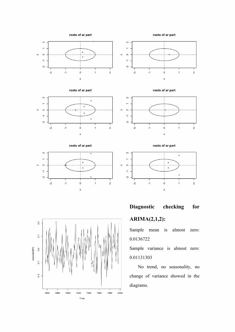
Diagnostic checking for

ARIMA(2,1,2):

Sample mean is almost zero:

0.0136722

Sample variance is almost zero:

0.01131303

No trend, no seasonality, no

change of variance showed in the

diagrams.

All acf and pacf of residuals are within confidence intervals and can be counted as zeros. 1.Box-Ljung test

data: residuals(fit4)

X-squared = 3.1663, df = 8, p-value = 0.9235

2.Box-Pierce test



3.Box-Ljung test

data: (residuals(fit4))^2


4.Shapiro-Wilk normality test


W = 0.985, p-value = 0.1229

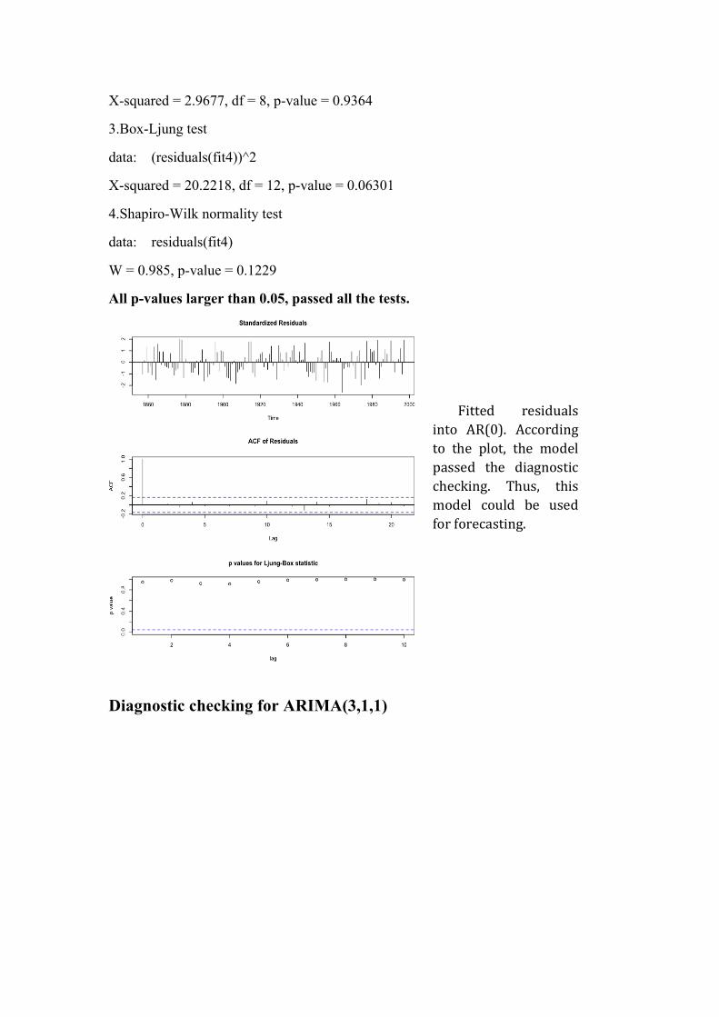
All p-values larger than 0.05, passed all the tests.

Diagnostic checking for ARIMA(3,1,1)

Fitted residuals into AR(0). According to the plot, the model passed the diagnostic checking. Thus, this model could be used for forecasting.

Mean almost zero: 0.0135089 variance almost zero: 0.01126948

No trend, no seasonality, no change of variance showed in the time series plot.

ALL ACF and PACF residuals are in the confidence intervals and can be counted

zero.

1.Box-‐Ljung test


X-‐squared = 2.4679, df = 8, p-‐value = 0.9632

2.Box-‐Pierce test



3.Box-‐Ljung test

data: (residuals(fit5))^2


4.Shapiro-‐Wilk normality test


W = 0.9846, p-‐value = 0.1117

ALL p-‐values larger than 0.05, passed all tests.

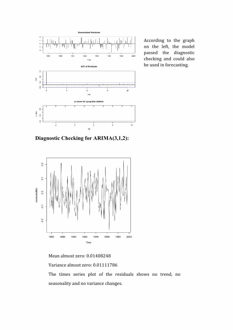
Diagnostic Checking for ARIMA(3,1,2):

According to the graph on the left, the model passed the diagnostic checking and could also be used in forecasting.

Mean almost zero: 0.01408248

Variance almost zero: 0.01111786

The times series plot of the residuals shows no trend, no

seasonality and no variance changes.

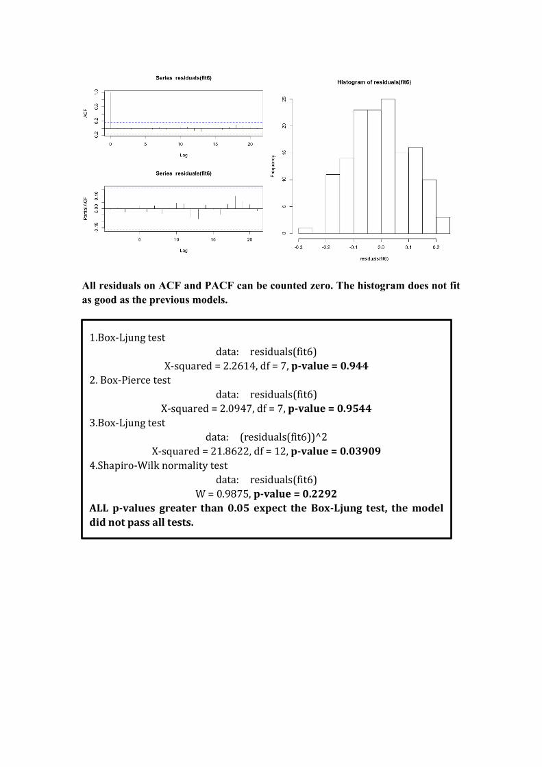
All residuals on ACF and PACF can be counted zero. The histogram does not fit as good as the previous models.

1.Box-‐Ljung test data: residuals(fit6)

X-‐squared = 2.2614, df = 7, p-‐value = 0.944 2. Box-‐Pierce test

data: residuals(fit6) X-‐squared = 2.0947, df = 7, p-‐value = 0.9544

3.Box-‐Ljung test data: (residuals(fit6))^2

X-‐squared = 21.8622, df = 12, p-‐value = 0.03909 4.Shapiro-‐Wilk normality test

data: residuals(fit6) W = 0.9875, p-‐value = 0.2292

ALL p-‐values greater than 0.05 expect the Box-‐Ljung test, the model did not pass all tests.

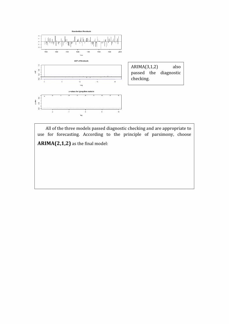
ARIMA(3,1,2) also passed the diagnostic checking.

All of the three models passed diagnostic checking and are appropriate to use for forecasting. According to the principle of parsimony, choose

ARIMA(2,1,2) as the final model:

Forecasting

Based on the model, we can get the following predictions. In which the difference

between the upper bond and the lower bond stands for the confidence interval, and the

points indicate the predictions of global land-air temperature in the future ten years.

According to the forecasting, it is observed that the temperature would decrease

slightly and steadily. Thus, we should not be worried too much about global warming

in the future 10 years.

III. References: Data source: CDIAC(Carbon Dioxide Information Analysis Center) website: http://cdiac.ornl.gov/trends/temp/jonescru/jones.html Investigators:

P. D. Jones1, D. E. Parker2, T. J. Osborn1, and K. R. Briffa1 1Climatic Research Unit, School of Environmental Sciences, University of East Anglia, Norwich NR4 7TJ, United Kingdom 2Hadley Centre for Climate Prediction and Research, Meteorological Office, Bracknell, Berkshire, United Kingdom

IV. Code: > library(tseries) > globtemp=ts(scan("/Users/camille/Desktop/globtemp.dat"), start=1856) > ts.plot(globtemp) # According to the time series plot, it is not stationary. > var(globtemp) V1 V1 0.04747083 > mean(globtemp) [1] -0.1580986 > par(mfrow=c(2,1)) > acf(globtemp,48) > acf(globtemp,type="partial",48) #According to the acf plot, the acf tails off slowly which indicates non-stationary. # First difference: Data is differenced at lag 1 in order to remove the trend. > globtempdiff1=diff(globtemp,1) > ts.plot(globtempdiff1) > mean(globtempdiff1) [1] 0.005602837 > var(globtempdiff1) V1 [1] 0.0146791 > par(mfrow=c(2,1)) > acf(globtempdiff1) > pacf(globtempdiff1) > library(qpcR) >library(forecast) #fit models

> fit1 = arima(globtemp, order = c(1,1,1), method = "ML") > fit2 = arima(globtemp, order = c(1,1,2), method = "ML") > fit3 = arima(globtemp, order = c(2,1,1), method = "ML") > fit4 = arima(globtemp, order = c(2,1,2), method = "ML") > fit5 = arima(globtemp, order = c(3,1,1), method = "ML") > fit6 = arima(globtemp, order = c(3,1,2), method = "ML") > fit7 = arima(globtemp, order = c(36,1,1), method = "ML") > fit8 = arima(globtemp, order = c(36,1,2), method = "ML") # Check the AICc > AICc(fit1) [1] -218.6715 > AICc(fit2) [1] -218.4678 > AICc(fit3) [1] -219.969 > AICc(fit4) [1] -218.5951 > AICc(fit5) [1] -219.1751 > AICc(fit6) [1] -218.5359 > AICc(fit7) [1] -150.8322 > AICc(fit8) [1] -149.093 # ARIMA(2,1,1) has the smallest AICc, ARIMA(1,1,1), ARIMA(1,1,2), ARIMA(2,1,2), ARIMA(3,1,1) and ARIMA(3,1,2) have similar AICc. #simulate models > fit3 Series: globtemp ARIMA(2,1,1) Coefficients: ar1 ar2 ma1 0.2846 -0.1848 -0.6950 s.e. 0.1222 0.0970 0.1009 sigma^2 estimated as 0.01156: log likelihood=114.07 AIC=-220.14 AICc=-219.85 BIC=-208.35 > fit1 Series: globtemp ARIMA(1,1,1) Coefficients:

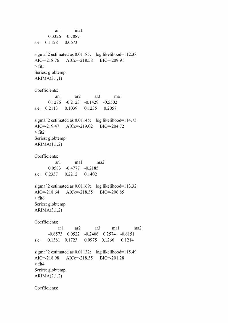
ar1 ma1 0.3326 -0.7887 s.e. 0.1128 0.0673 sigma^2 estimated as 0.01185: log likelihood=112.38 AIC=-218.76 AICc=-218.58 BIC=-209.91 > fit5 Series: globtemp ARIMA(3,1,1) Coefficients: ar1 ar2 ar3 ma1 0.1276 -0.2123 -0.1429 -0.5502 s.e. 0.2113 0.1039 0.1235 0.2057 sigma^2 estimated as 0.01145: log likelihood=114.73 AIC=-219.47 AICc=-219.02 BIC=-204.72 > fit2 Series: globtemp ARIMA(1,1,2) Coefficients: ar1 ma1 ma2 0.0583 -0.4777 -0.2185 s.e. 0.2337 0.2212 0.1402 sigma^2 estimated as 0.01169: log likelihood=113.32 AIC=-218.64 AICc=-218.35 BIC=-206.85 > fit6 Series: globtemp ARIMA(3,1,2) Coefficients: ar1 ar2 ar3 ma1 ma2 -0.6573 0.0522 -0.2406 0.2574 -0.6151 s.e. 0.1381 0.1723 0.0975 0.1266 0.1214 sigma^2 estimated as 0.01132: log likelihood=115.49 AIC=-218.98 AICc=-218.35 BIC=-201.28 > fit4 Series: globtemp ARIMA(2,1,2) Coefficients:

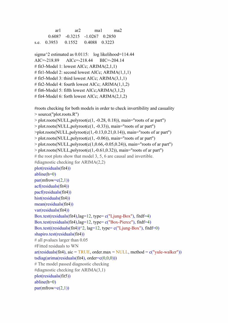
ar1 ar2 ma1 ma2 0.6087 -0.3215 -1.0267 0.2850 s.e. 0.3953 0.1552 0.4088 0.3223 sigma^2 estimated as 0.0115: log likelihood=114.44 AIC=-218.89 AICc=-218.44 BIC=-204.14 # fit3-Model 1: lowest AICc; ARIMA(2,1,1) # fit1-Model 2: second lowest AICc; ARIMA(1,1,1) # fit5-Model 3: third lowest AICc; ARIMA(3,1,1) # fit2-Model 4: fourth lowest AICc; ARIMA(1,1,2) # fit6-Model 5: fifth lowest AICc;ARIMA(3,1,2) # fit4-Model 6: forth lowest AICc; ARIMA(2,1,2) #roots checking for both models in order to check invertibility and casuality > source("plot.roots.R") > plot.roots(NULL,polyroot(c(1, -0.28, 0.18)), main="roots of ar part") > plot.roots(NULL,polyroot(c(1, -0.33)), main="roots of ar part") >plot.roots(NULL,polyroot(c(1,-0.13,0.21,0.14)), main="roots of ar part") > plot.roots(NULL,polyroot(c(1, -0.06)), main="roots of ar part") > plot.roots(NULL,polyroot(c(1,0.66,-0.05,0.24)), main="roots of ar part") > plot.roots(NULL,polyroot(c(1,-0.61,0.32)), main="roots of ar part") # the root plots show that model 3, 5, 6 are causal and invertible. #diagnostic checking for ARIMA(2,2) plot(residuals(fit4)) abline(h=0) par(mfrow=c(2,1)) acf(residuals(fit4)) pacf(residuals(fit4)) hist(residuals(fit4)) mean(residuals(fit4)) var(residuals(fit4)) Box.test(residuals(fit4),lag=12, type= c("Ljung-Box"), fitdf=4) Box.test(residuals(fit4),lag=12, type= c("Box-Pierce"), fitdf=4) Box.test((residuals(fit4))^2, lag=12, type= c("Ljung-Box"), fitdf=0) shapiro.test(residuals(fit4)) # all pvalues larger than 0.05 #Fitted residuals to WN ar(residuals(fit4), aic = TRUE, order.max = NULL, method = c("yule-walker")) tsdiag(arima(residuals(fit4), order=c(0,0,0))) # The model passed diagnostic checking #diagnostic checking for ARIMA(3,1) plot(residuals(fit5)) abline(h=0) par(mfrow=c(2,1))

acf(residuals(fit5)) pacf(residuals(fit5)) hist(residuals(fit5)) mean(residuals(fit5)) var(residuals(fit5)) Box.test(residuals(fit5),lag=12, type= c("Ljung-Box"), fitdf=4) Box.test(residuals(fit5),lag=12, type= c("Box-Pierce"), fitdf=4) Box.test((residuals(fit5))^2, lag=12, type= c("Ljung-Box"), fitdf=0) shapiro.test(residuals(fit5)) # all pvalues larger than 0.05 #Fitted residuals to WN ar(residuals(fit5), aic = TRUE, order.max = NULL, method = c("yule-walker")) tsdiag(arima(residuals(fit5), order=c(0,0,0))) # The model passed diagnostic checking ##diagnostic checking for ARIMA(3,2) plot(residuals(fit6)) abline(h=0) par(mfrow=c(2,1)) acf(residuals(fit6)) pacf(residuals(fit6)) hist(residuals(fit6)) mean(residuals(fit6)) var(residuals(fit6)) Box.test(residuals(fit6),lag=12, type= c("Ljung-Box"), fitdf=5) Box.test(residuals(fit6),lag=12, type= c("Box-Pierce"), fitdf=5) Box.test((residuals(fit6))^2, lag=12, type= c("Ljung-Box"), fitdf=0) shapiro.test(residuals(fit6)) # all pvalues larger than 0.05 #Fitted residuals to WN ar(residuals(fit6), aic = TRUE, order.max = NULL, method = c("yule-walker")) tsdiag(arima(residuals(fit6), order=c(0,0,0))) library(forecast) # Forecast next 10 observations of original time series pred <- predict(fit4, n.ahead = 10) pred.se<-pred$se ts.plot(globtemp,xlim=c(1856,2007),ylim=c(-0.5,0.7)) points((1998:2007),pred$pred,col="red") lines(1998:2007,pred$pred+1.96*pred.se,lty=2, col="black") lines(1998:2007,pred$pred-1.96*pred.se,lty=2, col="blue")

Documents

R language Project report