Quantum Diffusion and Delocalization for Random Band Matrices

Quantum Diffusion and Delocalization forRandom Band Matrices

Antti Knowles

Harvard University

Warwick – 12 January 2012

Joint work with Laszlo Erdos

Two standard models of quantum disorder

Consider the two random Hamiltonians on CN (one-dimensional lattice).Random Schrodinger operator. On-site randomness + short-range

hopping.

H = −∆ +∑x

vx =

v1 11 v2 1

1. . . . . .. . . vN−1 1

1 vN

Eigenvectors are localized, local spectral statistics are Poisson.

Wigner random matrix. H = (Hxy)Nx,y=1 with random centred entries,i.i.d. up to the constraint H = HT or H = H∗. This is a mean-fieldmodel with no spatial structure.

Eigenvectors are delocalized, local spectral statistics areGOE/GUE.

Antti Knowles Quantum Diffusion and Delocalization for Random Band Matrices 1

Band matrices

Intermediate model: random band matrix. The elements Hxy are centred,independent (up to H = H∗), and satisfy Hxy = 0 for |x− y| > W . Here Wis the band width.

Summary: If W = O(1) then H ∼ random Schrodinger operator.

If W = O(N) then H ∼Wigner matrix.


Anderson transition for band matrices

• W = O(1) =⇒ eigenvectors are localized.• W = O(N) =⇒ eigenvectors are delocalized.

Varying 1�W � N provides a means to test the Anderson transition.

Conjecture (numerics, nonrigorous SUSY arguments)

The Anderson transition occurs at W ∼ N1/2.

Let ` denote the typical localization length of the eigenvectors of H . Thenthe conjecture means that ` ∼W 2.

Rigorous results:• `/W 6W 7 (Schenker).• `/W >W 1/6 (Erdos, K).

Conjecture for higher dimensions

If d = 2 then ` is exponential in W .If d > 3 then ` = N (delocalization).


Assumptions

• Let d > 1 and N ∈ N. Consider random matrices H = (Hxy) whoseentries are indexed by x, y ∈ ΛN := {−N, . . . , N}d.

• Assume that the entries Hxy are independent (up to H = H∗) withvariances given by

E|Hxy|2 =1

W df

(x− yW

).

Here f is a probability density of zero mean on Rd (the “band shape”).• Assume that Hxy is symmetric and exhibits subexponential decay.

Note that∑y E|Hxy|2 = 1. Let {λα} be the family of eigenvalues of H .

Then

1

|ΛN |∑α

Eλ2α =

1

|ΛN |ETrH2 =

1

|ΛN |∑x,y

E|Hxy|2 = 1 ,

i.e. the eigenvalues of H are of order 1. In fact, Sp(H)→ [−2, 2].


The diffusive scaling

Define the quantum transition probability from 0 to x in time t through

%(t, x) := E∣∣⟨δx , e−itH/2δ0

⟩∣∣2 .Note that %(t, ·) is a probability on ΛN for all t.

Consider the diffusive regime

t = ηT , x = η1/2WX ,

for η →∞. Here X and T are of order one.

For d = 1, diffusion cannot hold for x�W 2 =⇒ choose η = Wκ for0 < κ < 2.


Quantum diffusion

Theorem(Quantum diffusion) [Erdos, K]

Fix 0 < κ < 1/3 and pick a test function ϕ ∈ Cb(Rd). Then

limW→∞

∑x∈ΛN

%(W dκT, x

)ϕ

(x

W 1+dκ/2

)=

∫Rd

dX L(T,X)ϕ(X) ,

uniformly in N >W 1+d/6 and T > 0 in compacts. Here

L(T,X) :=

∫ 1

0

dλ4

π

λ2

√1− λ2

G(λT,X)

is a superposition of heat kernels

G(T,X) :=1

(2πT )d/2√

det Σe−

12T X·Σ

−1X ,

where Σ = (Σij) is the covariance matrix of the probability density f :Σij :=

∫Rd dX XiXjf(X).


Interpretation of λ

The quantum particle spends a macroscopictime λT moving according to a randomwalk, with jump rate O(1) in time t andtransition kernel p(y ← x) = E|Hxy|2.The remaining fraction (1− λ)T is the timethe particle “wastes” in backtracking.Probability density of λ:

4

π

λ2

√1− λ2

0 0.2 0.4 0.6 0.8 1


Corollary: delocalization

Informally: fraction of eigenvectors localized on scales ` 6W 1+dκ/2

converges to 0.

Let {ψα}|ΛN |α=1 be an orthonormal family of eigenvectors of H . Fix K > 0and γ > 0 and define the random subset of eigenvectors

Bω` :=

{α ∈ A : ∃u ∈ ΛN

∑x

|ψωα(x)|2 exp

[|x− u|`

]γ6 K

}.

Theorem(Delocalization) [Erdos, K]

For any κ < 1/3 we have

limW→∞

E|B`||ΛN |

= 0 ,

where ` = W 1+dκ/2.

Proof. Expand e−itH/2δ0 =∑α ψα(0) e−itλα/2 ψα.


Naive (and doomed) attempt: power series expansion of e−itH/2

The moment method (Wigner 1955: semicircle law, . . . ) involvescomputing

ETrHn =∑

x1,...,xn

EHx1x2Hx2x3

· · ·Hxnx1

for large n. Because of EHxy = 0, nonzero terms have a complete pairing(or a higher-order lumping).

Graphical representation: path x1, x2, . . . , xn, x1.

• The path is nonbacktrackingif xi 6= xi+2 for all i.

• The path is fullybacktracking if it can beobtained from x1 bysuccessive replacements ofthe form a 7→ aba.(This generates“double-edged trees”.)


A fully backtracking path is paired byconstruction; its contribution is 1.

Proof. Sum over all vertices, startingfrom the leaves. Each summation yieldsa factor

∑y E|Hxy|2 = 1.

Fully backtracking paths give theleading order contribution as W →∞.Wigner’s original derivation of thesemicircle law involved counting thenumber of fully backtracking paths.

Applying this strategy to % leads to trouble: the expansion

%(t, x) =∑

n,n′>0

in−n′tn+n′

2n+n′n!n′!EHn

0xHn′

x0

is unstable as t→∞. The main contribution comes from fullybacktracking graphs, whose number is of the order 4n+n′ . The maincontribution to the sum over n, n′ comes from n+ n′ ∼ t (Poisson),diverges like e4t as t→∞.


Getting rid of the trees: perturbative renormalization

Simple example: Let z = E + iη with η > 0 and compute

EGii(z) = E(H − z)−1ii .

Assuming that the semicircle law holds, we know what to expect:

EGii(z) = E1

N

∑j

Gjj(z) = E1

N

∑α

1

λα − z= EmN (z) ≈ m(z)

where mN (z) is the Stieltjes transform of the empirical eigenvalue densityN−1

∑α δλα , and

m(z) :=

∫1

x− z

√4− x2

2πdx

is the Stieltjes transform of the semicircle law.

Note: m(z) is uniquely characterized by

z +m(z) +1

m(z)= 0 , |m(z)| < 1 (z /∈ [−2, 2]) .


Choose µ ≡ µ(z) ∈ C and expand G(z) around µ−1:

1

H − z=

1

µ+H − µ− z=

1

µ+

1

µ

∞∑n=1

(µ+ z

µ− H

µ

)n.

Thus we get

EGii =1

µ+

1

µ2(µ+ z) +

1

µ3

((µ+ z)2 + EH2

ii

)+

1

µ4(· · · ) + · · · .

Choose µ so that red terms cancel:

1

µ2(µ+ z) = − 1

µ3EH2

ii = − 1

µ3⇐⇒ z + µ+

1

µ= 0 .

We need |µ| > 1 for convergence: choose µ = m−1.

Using a graphical expansion, one can check that this choice of µ leads to asystematic cancellation of leading-order pairings (trees) up to all orders.What remains are higher-order corrections of size O(W−d). In particular,EGii = m+ o(1).

This is essentially two-legged subdiagram renormalization in perturbativefield theory. Works also for more complicated objects like E|Gij |2.


Renormalization using Chebyshev polynomials

A more systematic and powerful renormalization: use a beautifulalgebraic identity due to Bai, Yin, Feldheim, Sodin, . . . .

Define the n-th nonbacktracking power of H through

H(n)x0xn

:=∑

x1,...,xn−1

Hx0x1· · ·Hxn−1xn

n−2∏i=0

1(xi 6= xi+2) .

Assume from now on that

Hxy =1(1 6 |x− y| 6W )√

W dUnif(S1) .

We shall see later how to relax this condition.


Lemma[Bai, Yin]

H(n) = HH(n−1) −H(n−2)

Proof. Introduce 1 = 1(x0 6= x2) + 1(x0 = x2) into (HH(n−1))x0xn .

Feldheim and Sodin inferred that H(n) = Un(H), where Un(ξ) = Un(ξ/2)and Un is the standard Chebyshev polynomial of the second kind. Indeed,we have

Un(ξ) = ξUn−1(ξ)− Un−2(ξ) .

Thus, we expand the propagator e−itH/2 in terms of Chebyshevpolynomials:

e−itξ =∑n>0

αn(t)Un(ξ) .

We can compute the coefficients

αn(t) =2

π

∫ 1

−1

e−itξUn(ξ)√

1− ξ2 dξ = 2(−i)nn+ 1

tJn+1(t) ,

where Jn is the n-th Bessel function of the first kind.


The graphical representation

The Chebyshev expansion yields %(t, x) =∑

n,n′>0

αn(t)αn′(t)EH(n)0x H

(n′)x0 .

Represent matrix multiplication by loop;upper edge represents H(n)

0x and loweredge H(n′)

x0 .

Taking the expectation yields a lumping(or partition) Γ of the edges:

EH(n)0x H

(n′)x0 =

∑Γ∈Gn,n′

Vx(Γ) .

Each lump γ ∈ Γ contains at least twoedges.The most important lumpings are thepairings; their contribution estimates thecontribution of all other lumpings (seelater).


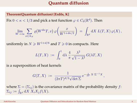
The ladder pairingsThe leading order contribution to % isgiven by the ladder pairingsL0, L1, L2, . . . :

%ladder(t, x) =∑n>0

|αn(t)|2 Vx(Ln)

The family of weights {|αn(t)|2}∞n=0 is at-dependent probability distribution on N(since the family {Un}∞n=0 is orthonormal).

The number |αn(t)|2 is the probability thatthe particle performs n steps of a randomwalk during the time t. The steps of therandom walk have the transition kernel

p(y ← x) = E|H2xy| =

1

W df

(x− yW

).

The distribution of the number of jumpsdoes not concentrate at n ≈ t because ofpossible delays due to backtracking.

0

2

4

6

8

10

0 0.2 0.4 0.6 0.8 1

The function λ 7→ t |α[λt](t)|2 fort = 150 (brown), and its weak limit4π

λ2√1−λ2

(blue) as t→∞.


The non-ladder lumpings

We have to prove that the sum of the contributions of all non-ladderlumpings vanishes. This is the main work!

• First, we estimate the contribution of all non-pairings in terms of thecontribution of all non-ladder pairings.=⇒ It is enough to show that the contribution of all non-ladderpairings vanishes as W →∞.

• Problem: The summation labels are associated with vertices, butedges are paired. We need to extract conditions on the vertex labelsfrom a pairing of the edges.

• Basic philosophy: The more complicated a pairing, the moreconstraints it induces on the vertex labels, and therefore the smaller itscontribution. This fights against the larger number of complicatedpairings.=⇒We need a means of quantifying the combinatorial complexity ofa pairing.

• Observation: A group of parallel lines has a large contribution, but atrivial combinatorics =⇒ parallel lines should not contribute to thecombinatorial complexity of a pairing.


Step 1. Collapse the parallel lines. We assign to each pairing Γ its skeletonpairing S(Γ) obtained from Γ by collapsing all parallel lines of Γ.

The size 2m of S(Γ) is the correct notion of complexity for Γ.

We recover Γ by replacing each line σ of S(Γ) with a number `σ of parallellines. The contribution of `σ parallel lines is given by a random walk with`σ steps =⇒ use heat kernel bounds on each line of S(Γ) (local CLT).

Step 2. Estimate the number of free labelsin a skeleton: the 2/3 rule. Since parallellines are forbidden, each vertex labelmust appear at least three times. Thus,the number L of free labels satisfies3L 6 2m, i.e. L 6 2m/3.


Step 3. Encode the skeleton as a multigraph and sum everything up usingheat kernel bounds.

Each edge σ of the multigraph carries a random walk of `σ steps. To sumup the graph, choose a spanning tree of the multigraph. Apply heat kernelbounds:

• `1-bound for each tree edge (→ factor 1)

• `∞-bound for each nontree edge (→ factor `−d/2σ W−d).

The 2/3 rule implies that the number of nontree edges is at least m/3.=⇒ Contribution of skeletons of size m is (roughly) bounded by(

n

m

)m! (W−d)m/3 .

This is summable for n 6 t�W d/3.Antti Knowles Quantum Diffusion and Delocalization for Random Band Matrices 19

The necessity of the condition κ < 1/3

The following family Σ1,Σ2,Σ3, . . . of skeletons is critical; Σk is defined as

The bound in the 2/3 rule is saturated: each vertex label occurs exactlythree times (6k edges and 4k free labels).

It is not hard to see that the contribution of all such skeletons diverges asκ→ 1/3.=⇒ going beyond κ = 1/3 requires (i) resummations of terms withdifferent n, n′, or (ii) a more refined use of heat kernel bounds.


General band matrices

So far we assumed that Hxy = W−d/21(1 6 |x− y| 6W ) Unif(S1), whichwas necessary for the algebraic identity

H(n) = HH(n−1) −H(n−2) (1)

to hold.

If the entries of H are general, the algebraic relation (1) is no longer exact;the RHS of (1) receives the error terms −Φ2H

(n−2) − Φ3H(n−3), where

(Φ2)xy := δxy∑z

(|Hxz|2 − E|Hxz|2

), (Φ3)xy := |Hxy|2Hxy .

Strategy: Φ3 is small by power counting (easy), Φ2 has zero expectation(hard).

The rigorous treatment requires a considerably more complicated class ofgraphs; out of the simple “loop” grow backtracking “branches”. Thecancellation of backtracking paths is no longer complete.

The organization of the expansion of the backtracking branches is quiteinvolved. The threshold t�W d/3 is again necessary.


Summary

• The quantum time evolution generated by e−itH/2 is diffusive up totime scales t�W d/3. The dynamics is given by a superposition ofdelayed heat kernels.

• Eigenvectors of H are delocalized on scales ` >W 1+d/6.

• Proof. Expansion in nonbacktracking powers H(n) of H ⇐⇒self-energy renormalization. Use that H(n) = Un(H). Control theexpectation using a graphical expansion.


Documents

Quantum Diffusion and Delocalization for Random Band Matrices