Embed Size (px)
Citation preview

DELOCALIZATION OF SCHRÖDINGER EIGENFUNCTIONS
NALINI ANANTHARAMAN
Abstract. A hundred years ago, Einstein wondered about quantization conditions forclassically ergodic systems. Although a mathematical description of the spectrum ofSchrödinger operators associated to ergodic classical dynamics is still completely missing,a lot of progress has been made on the delocalization of the associated eigenfunctions.
1. Some history
One can date the birth of quantum mechanics back to Planck’s 1900 paper [93], whenhe realized that the statistical model leading to the spectrum of the “black body” had tobe discrete, not continuous. To that effect, he introduced the “Planck constant” h, butthis was for him a mathematical artefact, without physical foundation. It was Einsteinwho gave this notion a physical meaning, introducing the idea of quantum of energy in theexchange of energy between electromagnetic field and matter (later called photon) [49].The amount of energy that can be exchanged between light of frequency ν and matter isdiscrete, “quantized”, it must be an integer multiple of hν.
This idea was applied by Bohr in 1913 to the planetary model of the atom [28]. Trying toexplain the discrete emission/absorption spectrum of the hydrogen, he used the Rutherfordmodel where the electron gravitates around the nucleus submitted to Coulomb attraction,and postulated the quantization of the kinetic momentum : it must be an integer multipleof h. This in turn implied that the energy can only take a discrete set of values, that fittedperfectly well with the experimental spectrum. However, setting up quantization rules forlarger atoms turned out to be an inextricable task.
In 1917, Einstein wrote a theoretical paper with an aim to extend the quantization rulesto systems with higher degrees of freedom [50]. He modified some rules given earlier byEpstein and Sommerfeld, and he noted that his new rules only made sense if (using modernvocabulary) the system is completely integrable : that is, if there exist some action/anglecanonical coordinates, such that the actions are invariants of motion (Einstein’s quantiza-tion rule is that the values taken by the action variables have to be integer multiples ofh). At the end of Einstein’s paper, there is a sentence that looks incidental, but may beconsidered to be the starting point of a whole field of research : “on the other hand, clas-sical statistical mechanics is essentially only concerned with Type b) [i.e. non integrablesystems], for in this case the microcanonical average is the same as the time average”.The equivalence of time average with the average over phase space is the property called“ergodicity”. Einstein’s point is the following : if a classical dynamical system is ergodic,the quantization rules do not apply, so how can we describe its spectrum ?
1

2 NALINI ANANTHARAMAN
Facing the failure to find quantization rules even for an atom as simple as the helium,Heisenberg set up in 1925 entirely new rules of mechanics [64]. One should work only withobservable quantities such as the position or the momentum (but for instance, the trajec-tory of an electron is not observable); and these “observables” are modelled by matrices(operators), subject to certain commutation rules. The momentum observable p and theposition observable q must satisfy qp − pq = iℏI, where ℏ is the reduced Planck constanth/2π. Time evolution is governed by the energy observable H; Heisenberg gives a recipeto build the operator H starting from the classical expression of energy. Any other observ-able A evolves according to the linear equation iℏdA
dt= [A,H], where [·, ·] stands for the
commutator of two operators. The physical spectrum of the system (emitted or absorbedenergies) is given by the differences En − Em, where (En) are the eigenvalues of H.
At the same time, a concurrent theory emerged. In 1923, De Broglie had formulated theidea of wave mechanics : in the same way as light, considered to be a wave, was discoveredto have a discrete behaviour embodied by the photons, one could do the reverse operationwith the particles composing matter, and consider them to be waves as well. In 1926Schrödinger proposed an evolution equation for a wave/particle of mass m evolving in aforce field coming from a potential V [99, 100] :
(1) iℏ∂ψ
∂t=
(− ℏ2
2m∆+ V
)ψ
where ∆ is the Laplacian, and where ψ = ψ(t, x) is a function of time t and of the positionx ∈ R3 of the particle, called the wave function.
The linear partial differential equation (1) can be solved by diagonalizing the differentialoperator H = − ℏ2
2m∆+ V . Assume, for instance, we can find an orthonormal basis of the
Hilbert space L2(R3) consisting of functions ϕn satisfying Hϕn = Enϕn with En ∈ R. Thenthe general solution of (1) is
ψ(t, x) =∑n
cnϕn(x)e−itEn/ℏ
where the coefficients cn ∈ C are given by the initial condition at t = 0. The physicalspectrum is again given by the differences En − Em.
Both the Heisenberg and the Schrödinger theories yielded exact results for the hydro-gen atoms, but also for larger ones. In fact, they can be shown to be mathematicallyequivalent. But, as Schrödinger wrote it [101], mathematical equivalence is not the sameas physical equivalence. The wave function ψ is absent from Heisenberg’s theory. Soonafterwards, Born gave a probabilistic interpretation of the function ψ : |ψ(x, t)|2 representsthe probability, in a measurement, to find a particle at position x, at time t. This was incomplete disagreement with Schrödinger’s intuition, but this is the interpretation that hasbeen retained.
After 1925, Einstein’s question may be reformulated as follows : if a classical system isergodic, and if H is the energy operator governing the system from the point of view ofquantum mechanics, what are the patterns exhibited by the eigenvalues of the operatorH ? How is classical ergodicity transferred to the quantum system ?

DELOCALIZATION 3
One may broaden the question by asking about the properties of the wave functions,that is, the eigenfunctions of H (solutions of Hϕ = Eϕ, E ∈ R), or more generally thesolutions ψ(x, t) of the time-dependent solutions of (1). How are the probability densities|ψ|2 localized in space ?
In the mid-fifties, Wigner introduced Random Matrix Theory to deal with the scatteringspectrum of heavy nuclei. Although there is no doubt about the validity of the Schrödingerequation, it seems impossible to effectively work with it, in view of the high number ofdegrees of freedom of such systems. Wigner’s hypothesis was that the spectrum of heavynuclei resembles, statistically, that of certain ensembles of large random matrices (theGaussian Orthogonal Ensemble or the Gaussian Unitary Ensemble). This turns out to fitthe experimental data extraordinarily well (pictures may be found in Bohigas’ paper [27]).
Unexpectedly, the spectral statistics of Random Matrix Theory were discovered to alsofit extremely well with the spectra of certain Schrödinger operators with very few degrees offreedom : the hydrogen atom in a strong magnetic field, as well as some 2-dimensional bil-liards (in the latter case, the Schrödinger operator is just the Laplacian in a bounded openset of R2, with Dirichlet boundary condition). See Delande’s paper [43] for illustrations.The common point of all these examples is that the underlying classical dynamical systemis ergodic, or even chaotic, meaning a very strong sensitivity to initial conditions. So, itseems that the answer to Einstein’s question could be that : if the classical dynamics is er-godic, or sufficiently chaotic, then the spectrum of the corresponding Schrödinger operatorlooks like that of a large random matrix. This is known as the Bohigas–Giannoni-Schmitconjecture [26]. However, :
• there is to this day no mathematical proof of this fact; the question may be con-sidered fully open, except for the heuristic arguments given by Sieber and Richter[103], that seem impossible to make mathematically rigourous;
• there are some counter-examples to this assertion, given by Luo and Sarnak [87];and they come from very strongly chaotic classical dynamics, so the source of theproblem does not lie there.
The counter-examples are Laplacians on arithmetic hyperbolic surfaces (such as the mod-ular surface and finite covers thereof); they are believed to be “non-generic” in some vaguesense, and thus one may conjecture that the assertions above hold for “generic” systems.But even in such a weakened form, the question is fully open.
On the other hand, the question of localization of wave functions, although very difficult,has known steady progress in the last decade. In this paper, we will
• report on recent progress on delocalization of wave functions for chaotic systems,in the semiclassical limit (limit of small wavelengths), Section 2;
• discuss delocalization of eigenfunctions on large finite systems, such as large finitegraphs, or Riemann surfaces of high genus, Sections 3 and 4;
• find a link between spatial delocalization and spectral delocalization on infinitesystems, §3.4;
• note that delocalization of eigenvectors of large random matrices has also under-gone intensive study lately. Although these eigenvectors have no direct physical

4 NALINI ANANTHARAMAN
interpretation, they are directly related to the Green function and were studied inrelation with the question of universality of the spectrum. The spectacular recentprogress on Wigner matrices and large random graphs will be mentioned in §4.1– in a largely non exhaustive manner, as we will focus on results pertaining todelocalization of eigenvectors.
2. High frequency delocalization
In this section, we let (M, g) be a compact smooth Riemannian manifold of dimension d,and ∆ be the Laplace-Beltrami operator on M . It is a self-adjoint operator on the Hilbertspace L2(M,Vol), where Vol is the Riemannian volume measure. We diagonalize ∆ : itis known that there is a non-decreasing sequence λ0 = 0 < λ1 ≤ λ2 ≤−→ +∞, and anorthonormal basis (ϕk)k∈N of L2(M,Vol), such that
∆ϕk = −λkϕk.
If M has a boundary, we impose a boundary condition, for instance the Dirichlet con-dition (i.e. we ask that ϕk vanishes on ∂M). The case when M is a billiard table, thatis, a bounded domain in R2 with piecewise smooth boundary, already contains all the dif-ficulties of the subject : actually, the presence of a boundary induces additional technicaldifficulties, and all the theorems given below have been proven for boundariless manifoldsfirst.
In this part of the paper, we are interested in notions of delocalization defined in thehigh-frequency limit λk −→ +∞. This is the same as the small wavelength limit, andit is also known as a semiclassical limit, meaning that classical dynamics emerges fromquantum mechanics in this limit.
Figure 1. Plot of |ϕn(x, y)|2 for the stadium billiard with odd-oddsymmetry, for consecutive states starting from n = 319. Darker shadescorrespond to large values of the eigenfunctions. Courtesy A. Bäcker
2.1. The role of the geodesic flow . The eigenfunction equation ∆ϕk = −λkϕk may berewritten as −ℏ2∆ϕ = Eϕ (with λk = Eℏ−2) to make a connection with the Schrödingeroperators from (1) (so the external potential V vanishes here). If we impose that E staysaway from 0, the limit λk −→ +∞ is equivalent to ℏ −→ 0; in this régime, quantum

DELOCALIZATION 5
mechanics should “converge to classical mechanics”. This was actually a requirement ofSchrödinger when he introduced his equation [100].
The Schrödinger operator −ℏ2∆ corresponds to a particle moving on M in absence ofany external force. In classical mechanics, this corresponds to the motion along geodesics,in other words, the motion with zero acceleration. When M is a billiard, the motion is instraight line, with reflection on the boundary. We denote by T ∗M the cotangent bundle ofM ; this is the classical phase space. An element (x, ξ) ∈ T ∗M has a component x ∈ M(the “position” of the particle) and ξ ∈ T ∗
xM (the “momentum”). For (x, ξ) ∈ T ∗M , andt ∈ R, we denote by gt(x, ξ) ∈ T ∗M the position and momentum of the particle, after it hasmoved during time t along the geodesic starting at x with initial momentum ξ. The family(gt)t∈R : T ∗M −→ T ∗M is a flow of diffeomorphisms, meaning that gt+s = gt gs and g0 isthe identity. This dynamical system is called the geodesic flow. The motion along geodesicshas constant speed, and thus, the unit cotangent bundle S∗M = (x, ξ) ∈ T ∗M, ∥ξ∥x = 1is preserved by gt.
In the limit of small wavelengths, (λk −→ +∞), the Schrödinger equation∂ψ
∂t= i∆ψ
moves the wavefronts along geodesics. What we mean is that, if we start with an initialcondition of the special form
ψϵ(x) = χ(x)eiS(x)ϵ
with χ and S smooth, and apply the unitary group eiϵt∆ (note the rescaling of time), theneiϵt∆ψϵ is of the form
(2) eiϵt∆ψϵ(x) = χt(x)eiS(t,x)
ϵ +Ot(ϵ)
where• S(t, x) satisfies the Hamilton-Jacobi equation ∂S
∂t= ∥dxS∥2; which means that at
time t the “wavefront set” (x, dxS(t, x)) ⊂ T ∗M is the image under gt of theinitial wavefront set (x, dxS(x));
• denoting Gt : x 7→ πgt(x, dxS), where π : T ∗M −→ M is the projection to theposition coordinate, we have
χt(y) = χ(G−ty)|G−ty|1/2
where |G−ty| is the Jacobian of the map G−t at y. This normalization factor isrelated to the fact that the L2 norm must be constant in time.
Formula (2) is an approximate one, it has a remainder term Ot(ϵ). It is called a BKWapproximation, as it was first obtained by Brillouin, Kramers, Wentzell [79, 115, 35]. Notethat this description is usually only valid for small times; for larger times, it might nolonger be possible to write the set gt(x, dxS(x)) in the form (x, dxS(t, x)) for somesmooth function S(t, ·), as caustics may appear.
Using (2), and the fact that eigenfunctions satisfy eiϵt∆ϕk = e−iϵtλkϕk, we can hopeto establish a relation between the behaviour of the eigenfunctions and the large-timeproperties of the geodesic flow, however there are two main difficulties :

6 NALINI ANANTHARAMAN
– a general function ϕ is not of the form (2), but can be written as a linear superposition ofsuch functions (with ϵ ∼ λ
−1/2k in the case of eigenfunctions). This may be seen using the
Fourier transform in local coordinates. It is extremely difficult to control how the differentterms will add up and interfere after applying eiϵt∆, for large t;– the error term in (2) grows (usually exponentially) with t; so it is extremely delicate touse the approximation (2) for large times.
2.2. Lp-norms as measures of delocalization ? One of the first question that comesto mind at the sight of Figure 1 is : how large can the eigenfunctions be, how stronglycan they be peaked, and at what points ? In this section we denote by ϕλ any solutionof −∆ϕλ = λϕλ, normalized so that ∥ϕλ∥L2 = 1. A general bound on the L∞-norm is thefollowing :
Theorem 1. (known as Hörmander’s bound)
∥ϕk∥∞ = O(λ(d−1)/4k ).
In a celebrated paper, C. Sogge gave a bound for all Lp norms, 2 ≤ p ≤ +∞ :
Theorem 2 (Sogge, [107]).∥ϕλ∥Lp = O(λ
µ(p)2 )
where• µ(p) = d
(12− 1
p
)− 1
2for 2(d+1)
(d−1)≤ p ≤ +∞;
• µ(p) = d−12
(12− 1
p
)for 2 ≤ p ≤ 2(d+1)
(d−1).
These bounds hold for any compact manifold M . Recall that d is the dimension ofM . Note the role of the critical value pc = 2(d+1)
(d−1). The upper bounds are achieved on
the sphere Sd : with zonal spherical harmonics for p ≥ pc (these spherical harmonics arestrongly peaked at 2 poles), and with highest weight spherical harmonics for p ≤ pc (thesespherical harmonics are peaked in the vicinity of a circle). So, in all the Lp-norms, thesphere is a case where eigenfunctions are most strongly peaked. For p > pc, several resultsgive a partial converse, showing that manifolds where the Lp-bound is saturated must havea “pole”, that is, a point where many geodesics loops go through :
If x ∈M , let Lx ⊂ S∗xM be the set of directions that loop back to x, i.e.Lx = v ∈ S∗
xM, ∃t > 0, gt(x, v) ∈ S∗xM.
We denote by σx the Lebesgue measure on the sphere S∗xM .
Theorem 3 (Sogge-Zelditch [108, 109, 110]). • Assume there exists a subsequence λnk−→
+∞ and C > 0 such that ∥ϕλnk∥∞ ≥ Cλ
µ(∞)2 . Then there exists x such that
σx(Lx) > 0;• If M is real analytic, the existence of such subsequence ϕλnk
is equivalent to theexistence of x such that Lx = S∗
xM , and the first return map ηx : S∗xM −→ S∗
xMpossesses an absolutely continuous invariant probability measure. (Moreover, in

DELOCALIZATION 7
that case, there exists t0 > 0 such that gt0(x, v) ∈ S∗xM for all v ∈ S∗
xM , that is,there is a common return time).
• If M is real analytic and dimM = 2, the existence of such subsequence ϕλnkis
equivalent to the existence of x ∈ M and t0 > 0 such that gt0(x, v) = (x, v) for allv ∈ S∗
xM .
What about our original question ? is it true that, if the geodesic flow is chaotic, eigen-functions will be much less peaked ? To be more specific, we shall mostly be interested inmanifolds with negative sectional curvatures. It is then known that the geodesic flow hasthe Anosov property, which is a very strong and very well understood form of chaos : thegeodesic flow is not only ergodic, it has strong mixing properties, is measurably isomorphicto a Bernoulli system, exhibits exponential sensitivity to initial conditions,... On a nega-tively curved manifold, there are only countably many closed geodesic, and what’s more,through a point x there pass at most countably many geodesic loops. Thus, Theorem 3implies that ∥ϕλ∥L∞ = o
(λ
µ(∞)2
)(the big O if Theorem 1 becomes a little o).
One can in fact go further :
Theorem 4. (i) (Bérard 1977 [17]) If d = 2 and M has no conjugate points, or if d ≥ 2and M has non-positive sectional curvature, for p = +∞,
∥ϕλ∥Lp = O
(λ
µ(p)2
√log λ
).
(i’) (Bonthonneau [30]) Statement (i) actually holds if M has no conjugate points, forall d ≥ 2.
(ii) (Hassell-Tacy [63]) (i) holds for all p > pc.(iii) (Blair-Sogge [24, 22]) If M has non-positive sectional curvature, for p < pc, there
exists σ(p, d) > 0 such that
∥ϕλ∥Lp = O
(λ
µ(p)2
(log λ)σ(p,d)
)(iv) (Blair-Sogge [23]) Statement (iii) still holds for p = pc.
(iii) and (iv) were previously proven by Hezari and Rivière [67] for negatively curvedmanifolds and for a density 1 sequence of eigenfunctions.
Although this logarithmic improvement constitutes a great progress, it is far from reach-ing our goal of saying that eigenfunctions are “spread around” if the geodesic flow is chaotic.In fact, after all it is only assumed that the curvature is non-positive, so the results holdalready for flat tori (where the geodesic flow is completely integrable), and has not muchto do with the long-term chaotic behaviour of the geodesic flow.
2.3. The Shnirelman theorem and the Quantum Unique ergodicity conjecture .As another indicator of delocalization, we can study the probability measure |ϕk(x)|2dVol(x).Ideally, the aim is to show that it is close to the uniform measure (say, asymptotically asλk −→ +∞); or, maybe less ambitiously we could ask whether the measure |ϕk(x)|2dVol(x)

8 NALINI ANANTHARAMAN
can be large on “small” sets (sets of small dimension for instance). The Quantum Ergod-icity theorem gives a first and almost complete answer in case the geodesic flow is ergodic,with respect to the Liouville measure.
Recall, this means that for any L1-function a : S∗M −→ R, for Lebesgue almost-every (x0, ξ0) ∈ S∗M , the time average 1
T
∫ T
0a gt(x0, ξ0)dt converges as T −→ +∞ to
the phase-space average∫S∗M
a dL where L is the normalized Liouville measure on S∗M(i.e. the Lebesgue measure, the uniform measure), arising naturally from the symplecticstructure on T ∗M .
Quantum Ergodicity Theorem (Shnirelman theorem).
Theorem 5 (Shnirelman, Zelditch, Colin de Verdière [106, 40, 116]). Let (M, g) be acompact Riemannian manifold, with the metric normalized so that Vol(M) = 1. Call ∆the Laplace-Beltrami operator on M . Assume that the geodesic flow of M is ergodic withrespect to the Liouville measure. Let (ϕk)k∈N be an orthonormal basis of L2(M, g) made ofeigenfunctions of the Laplacian
∆ϕk = −λkϕk, λk ≤ λk+1 −→ +∞.
Let a be a continuous function on M . Then
(3) 1
N(λ)
∑k,λk≤λ
∣∣∣∣⟨ϕk, aϕk⟩L2(M) −∫M
a(x)dVol(x)
∣∣∣∣2 −→λ−→+∞
0
where the normalizing factor is N(λ) = |k, λk ≤ λ|.
Note that ⟨ϕk, aϕk⟩L2(M) =∫Ma(x)|ϕk(x)|2dVol(x).
Remark 6. The Cesaro limit (3) implies that there exists a subset S ⊂ N of density 1such that
(4) ⟨ϕk, aϕk⟩ −→n−→+∞,n∈S
∫M
a(x)dVol(x).
In addition, using the fact that the space of continuous functions is separable, one canactually find S ⊂ N of density 1 such that (4) holds for all a ∈ C0(M). In other words,the sequence of measures (|ϕk(x)|2dVol(x))n∈S converges weakly to the uniform measuredVol(x).
Actually, the full statement of the theorem says that there exists a subset S ⊂ N ofdensity 1 such that
(5) ⟨ϕk, Aϕk⟩ −→n−→+∞,n∈S
∫S∗M
σ0(A)dL
for every pseudodifferential operator A of order 0 on M . On the right-hand side, σ0(A) isthe principal symbol of A, that is a function on the unit cotangent bundle S∗M . Equation4 corresponds to the case where A is the operator of multiplication by the function a.

DELOCALIZATION 9
The theorem has subsequently been extended to manifolds with boundary [57, 119]. Itapplies, in particular, to the stadium billiard in Figure 1, where the billiard flow has beenproven by Bunimovich to be ergodic. The observation of large samples of eigenfunctionsreveals that, indeed, most eigenfunctions are uniformly distributed over the stadium, butsome of them look very localized inside the rectangle, and some of them also exhibit somemild enhancement in the neighbourhood of unstable periodic orbits, a phenomenon called“scarring” by physicists (Heller,[66]).
The theorem was also extended to general Schrödinger operators (or even pseudodifferen-tial operators) in the limit ℏ −→ 0 [65]; more recently, to systems of differential operatorsacting on sections of vector bundles – such as Dirac operators, Dolbeault Laplacians,...[29, 71, 72]. The case of metrics with jump-like discontinuities has been elucidated [70],as well as the case of pseudo-riemannian Laplacians on 3-dimensional contact manifolds(for instance, the Laplacian on the Heisenberg group or its quotients) [42]. “Small scalequantum ergodicity”, that is, the possibility to use in (3) a test function a whose supportshrinks as λk −→ +∞, has been explored in [67, 60] on negatively curved manifolds, andon flat tori in [61, 83].
Quantum Unique Ergodicity conjecture. One may wonder whether the full se-quence converges in (5), without having to extract the subsequence S. Figure 1 (or largersamples of eigenfunctions) suggests that this is not the case for the billiard stadium, wherewe see a sparse sequence of eigenfunctions that are not at all equidistributed.
This was proven by Hassell in 2008 [62] (for “almost all” stadium billiards, meaning, forLebesgue-almost-all lengths of the stadium).
On the other hand, Rudnick and Sarnak’s Quantum Unique Ergodicity (QUE) conjec-ture [95] predicts that if M is a compact boundaryless manifold with negative sectionalcurvatures, then one has convergence of the full sequence in (5), in other words the wholesequence of eigenfunctions becomes equidistributed as λ −→ +∞. The conjecture hasbeen proved by Lindenstrauss in the setting of “Arithmetic Quantum Unique Ergodic-ity”, where M is an “arithmetic” hyperbolic surface, and where the ϕλ are assumed to beeigenfunctions, not only of the Laplacian, but also of the Hecke operators [84, 34, 39].
Arithmetic Quantum Unique Ergodicity will not be discussed with enough detail in thistext, but the results have been presented at previous ICM’s; we refer to [98, 48, 85, 111]for a more adequate overview.
For general negatively curved manifolds, the conjecture is open, but in the last 20 yearssignificant progress has been made :
2.4. Entropy and support of semiclassical measures. In this section, M is assumedto have negative sectional curvature, and dimension d.
Let us come back to the diagonal matrix elements ⟨ϕn, Aϕn⟩ appearing in (5), where Ais a pseudodifferential operator of order 0. By a general compactness argument, one mayalways extract subsequences so that ⟨ϕnk
, Aϕnk⟩ converge for all A. The limit is of the form∫
S∗Mσ0(A)dµ, where µ is a probability measure on S∗M . A measure obtained this way
is obtained, according to sources, “microlocal defect measure”, “semiclassical measure”,

10 NALINI ANANTHARAMAN
or “microlocal lift” associated with the sequence ϕnk. The Quantum Unique Ergodicity
conjecture described above is equivalent to proving that µ has to be the Liouville measure,for every subsequence (ϕnk
). But without aiming that far, we can try to characterizespecific properties of the measure µ. A priori, we only know that µ has to be invariantunder the geodesic flow : that is, gt♯µ = µ for all t ∈ R. This is a consequence of theeigenfunction property and of the classical/quantum correspondence as λ −→ +∞, as seenin §2.1.
Theorem 7. [3] Assume M is a compact Riemannian manifold with negative sectionalcurvature. Assume ⟨ϕnk
, Aϕnk⟩ converges to
∫S∗M
σ0(A)dµ for all A. Then µ has positiveentropy.
This is the Kolmogorov-Sinai entropy of dynamical systems. We do not give its definitionhere, but state a few facts to help understand the implications of the theorem. To eachinvariant probability measure ν of a dynamical system (here the geodesic flow), one canassociate a non-negative number hKS(ν), having the following properties :
• if ν is carried by a periodic trajectory, then hKS(ν) = 0;• ν 7→ hKS(ν) is affine : hKS(αν1 + (1− α)ν2) = αhKS(ν1) + (1− α)hKS(ν2), for any
invariant measures ν1, ν2, for α ∈ [0, 1];• (Pesin-Margulis-Ruelle inequality) if the dynamical system is sufficiently smooth,
(6) hKS(ν) ≤∫ ( r∑
j=1
χ+j (ρ)
)dν(ρ)
where the numbers χ+j (ρ) are the positive Lyapunov exponents of a point ρ – defined
ν-almost everywhere, by the Oseledets theorem – that give the rate of exponentialinstability of the trajectory of ρ.
• in the case of the geodesic flow on a negatively curved manifold, there is equalityin (6) if and only if ν is the Liouville measure L (Ledrappier-Young [81, 82]);
• in the case of the geodesic flow on a negatively curved manifold, of constant cur-vature −1 and dimension d (so that S∗M has dimension 2d − 1), there are d − 1positive Lyapunov exponents, they do not depend on ρ and have the value 1. Thus,(6) can be written as
(7) hKS(ν) ≤ d− 1,
with equality if and only if ν is the Liouville measure L.Let us give two more transparent corollaries to Theorem 7 :
Corollary 1. Let Γ ⊂ S∗M be the union of all points lying on a periodic trajectory onthe geodesic flow (recall, if M has negative curvature, there are countably many periodicgeodesics). Let µ be as in Theorem 7. Then µ(Γ) < 1.
Otherwise, µ would have zero entropy. In the physics literature, an eigenfunction that isenhanced near an unstable periodic classical trajectory is said to have a scar (Heller, [66]).In the mathematics literature, a sequence of eigenfunctions is said to be strongly scarred

DELOCALIZATION 11
if the corresponding semiclassical meaure µ is supported on some periodic trajectory. Ourtheorem thus shows that this is not possible on a negatively curved manifold (however, itdoes not rule out a partial scar , that is to say that µ(Γ) > 0).
From the definition of entropy, one can also prove :
Corollary 2. The support of µ has Hausdorff dimension > 1.
Note that the fact that the dimension is ≥ 1 is trivial since µ is invariant under thegeodesic flow.
With Nonnenmacher, we later obtained a more quantitative version if the curvature isconstant.
Theorem 8 (Anantharaman-Nonnenmacher [7]). Assume M is a compact Riemannianmanifold of dimension d, with constant sectional curvature −1. Then µ has entropy greaterthan d−1
2.
By the aforementioned properties of entropy, the QUE conjecture in constant negativecurvature is equivalent to proving that µ has entropy d − 1, so we fall short of a factor1/2. There are toy models of quantum chaos where it is known that the lower bound d−1
2is sharp, i.e. there are sequences of eigenfunctions that are not equistributed and haveexactly half the maximal entropy : see the quantum cat map and the quantum baker’smap [55, 6].
Corollary 3. The support of µ has Hausdorff dimension ≥ d.
As a comparison, the dimension of the full phase space T ∗M is 2d, and of the energylayer S∗M is 2d− 1.
Corollary 4. Let Γ ⊂ S∗M be the union of all points lying on a closed trajectory on thegeodesic flow. Let µ be as in Theorem 7, with M of constant negative curvature. Thenµ(Γ) ≤ 1/2.
Indeed, let us decompost µ as µ = αµ1 + (1 − α)µ2, where µ1 is carried by Γ, so thathKS(µ1) = 0. So hKS(µ) = (1 − α)hKS(µ2). The result says that this has to be ≥ d−1
2;
but the entropy of µ2 is smaller than the maximal entropy d − 1, so necessarily α ≤ 1/2.For the toy model of the quantum cat map, Corollary 4 had been proven by Faure andNonnenmacher in [54] without using entropy.
In variable curvature, the generalization of Theorem 8 should be that the entropy ofµ is greater than 1
2
∫S∗M
∑d−1j=1 χ
+j dµ, where χ+
j are the Lyapunov exponents. Howeverour method in [7] gives a slightly less good bound; the predicted lower bound in variablecurvature has only been obtained for d = 2, by G. Rivière [94]. Again, by the Ledrappier-Young theorem [81], proving QUE is equivalent to getting rid of the factor 1/2 in Rivière’sresult.
Theorem 9 (Dyatlov-Jin [47]). µ has full support, that is, µ(Ω) > 0 for any non-emptyopen set Ω ⊂ S∗M .

12 NALINI ANANTHARAMAN
Note that Theorems 7 and 9 are somehow independent. There are measures with positiveentropy and not full support (for instance, measures supported by geodesics avoiding anopen set Ω may have a large entropy). And there are measures having full support but zeroentropy (for instance, a measure putting positive weight on each periodic geodesic). Bothresults leave open the question whether µ can be a convex combination of the Liouvillemeasure and a measure carried on a closed geodesic. Such limit measures appeared in theaforementioned toy models of quantum chaos [55].
2.5. Some questions on non-compact manifolds. We have chosen to limit the scopeof this text to compact manifolds (and thus, “delocalization” is understood in the limit ofsmall wavelength, but does not deal with what happens at infinity). There are of coursemany interesting questions related to delocalization phenomena on non-compact manifolds,that we briefly review in this paragraph.
In keeping with the rest of this paper, let us consider the Laplacian on a non-compactriemannian manifoldM (most questions also make sense for general Schrödinger operators).
2.5.1. Absolutely continuous spectrum . In the context of infinite systems, the word “de-localization” is often used to mean that the Laplacian has no pure-point spectrum (thismeans that eigenfunctions are not square-integrable), or even stronger, purely absolutelycontinuous spectrum, in some region of the spectrum.
As we will see in §4.3, one can sometimes prove that this implies a form of “quantumergodicity” for eigenfunctions on large compact manifolds approximating M (see Theorem22 for a precise statement). For the moment, this theorem is restricted to the case whereM is the hyperbolic disc, where the spectrum of the Laplacian is explicit and can be seen(by direct computation) to be purely absolutely continuous. In general, it turns out to bevery difficult to find examples of M having purely absolutely continuous in some interval ofthe L2-spectrum, outside of the world of locally symmetric spaces. For instance, startingfrom X a compact riemannian manifold with variable negative sectional curvature, andtaking M = X to be its universal cover, it seems that nothing is known about the natureof the spectrum of the Laplacian on M , although one would be naturally inclined to guessthat is has absolutely continuous spectrum.
2.5.2. Large frequency delocalization on non-compact manifolds. If ϕλ is a solution of−∆ϕλ = λϕλ on M (with λ ∈ R) one could ask the question of the behaviour of themeasures |ϕλ(x)|2dVol(x), in the limit λ −→ +∞, even if M is non-compact. More pre-cisely, it seems reasonable to restrict these measures to a compact set before studying thislimit.
When M is a finite volume hyperbolic surface – so that the ends of M are hyperboliccusps – the question was studied by Zelditch in [117], for ϕλ generalized eigenfunctionscorresponding to the absolutely continuous spectrum : the so-called Eisenstein series. A“quantum ergodicity” theorem was proven. It was strengthened to a “quantum uniqueergodicity” result by Jakobson in [69], when M is the modular surface. When M has vari-able curvature in a compact subset, but still has hyperbolic cusps, quantum ergodicity wasproven more recently in [31]. Note that for infinite volume, convex-cocompact manifolds,

DELOCALIZATION 13
quantum (unique) ergodicity for the Eisenstein series has been studied in [46, 59, 68] butthe phenomena are quite different, as it is not the Liouville measure that appears at thesemiclassical limit, but a family of measures indexed by the boundary at infinity.
Back to the case of finite volume hyperbolic surface, an example of special interest innumber theory is the modular surface and its congruence covers. In this case, M has aninfinite sequence of discrete eigenvalues embedded in the continuous spectrum (see thesurvey papers [96, 98] for more details and references). “Arithmetic quantum ergodicity”is the study of the joint L2-eigenfunctions of the Laplacian and of the so-called “Heckeoperators”. In this context, Arithmetic Quantum Unique ergodicity, that is, the conver-gence of the full sequence of probability measures |ϕλ(x)|2dVol(x) to a multiple of theuniform measure, was proven by Lindenstrauss [84]. Since the modular surface is not com-pact, there can be escape of mass to infinity, and thus it is not clear that the limit of themeasures |ϕλ(x)|2dVol(x) is still a probability measure. Escape of mass was ruled out bySoundararajan [112].
Having discrete spectrum embedded in the continuous spectrum is non-generic. Forgeneral hyperbolic surfaces, the discrete spectrum is turned into the “resonance spectrum”;resonances are poles of the analytic continuation on the resolvent restricted to C∞
c (M)[102, 32]. Generically, resonances are not real. Naturally attached to resonances, thereare non-L2-eigenstates called “resonant states”. The question of quantum ergodicity forresonant states is to this date fully open, and seems extremely difficult.
3. Large scale delocalization
In the mathematical physics literature, it is believed that the spectrum of the Laplacian,as well as its eigenfunctions, should exhibit universal features that depend only on qual-itative geometric properties of the space. Localization/delocalization of eigenfunctions isbelieved to bear close relation with the nature of spectral statistics : localization is sup-posedly associated with Poissonian spectral statistics, whereas delocalization should beassociated with Random Matrix statistics (GOE/GUE). In the field of quantum chaos,the former notion is often associated with integrable dynamics and the latter with chaoticdynamics [21, 26]. However, specific examples show that the relation is not so straight-forward [87, 96, 97, 88]. Understanding how far one can push these ideas is one amongstmany reasons for studying models of large graphs as toy models [73, 77, 78, 104, 105].
It seems that “quantum graphs” have been studied before discrete graphs in the contextof quantum chaos. By “quantum graphs”, we mean 1-dimensional CW-complexes with∆ = d2
dx2 on the edges and suitable matching conditions on the vertices; the most naturalones being the “Kirchhoff” matching condition where it is asked that the functions arecontinuous at the vertices, and that the sum of their derivatives at a vertex vanish. On afixed quantum graph, it is known that the analogue of Shnirelman’s theorem never holdsin the large frequency limit λ −→ +∞ [41]. See also [19, 74, 58, 18] for other resultspertaining to eigenvalue or eigenfunction statistics on compact quantum graphs.
In what follows, instead of the high-frequency limit, we consider the limit where the sizeof the graph goes to infinity (“large scale limit”). We focus on discrete graphs and the

14 NALINI ANANTHARAMAN
eigenfunctions of their adjacency operators – although similar questions for large quantumgraphs should also be explored in the future. We mostly focus on discrete regular graphs,but in §3.4 also report on recent progress concerning non-regular graphs.
3.1. Overview of the problem. Consider a very large graph G = (V,E). Are theeigenfunctions of its adjacency matrix localized, or delocalized ? These words are used in avariety of contexts, with several different meanings.
For discrete Schrödinger operators on infinite graphs (e.g. for the celebrated Ander-son model describing the metal-insulator transition), localization can be understood in aspectral, spatial or dynamical sense. Given an interval I ⊂ R, one can consider
• spectral localization : pure point spectrum in I,• exponential localization : the corresponding eigenfunctions decay exponentially,• dynamical localization : an initial state with energy in I which is localized in a
bounded domain essentially stays in this domain as time goes on.On the opposite, delocalization may be understood at different levels :
• spectral delocalization : purely absolutely continuous spectrum in I,• ballistic transport : wave packets with energies in I spread on the lattice at a specific
(ideally, linear) rate as time goes on.Here we want to discuss notions of spatial delocalization. Since the wavefunctions corre-sponding to absolutely continuous spectrum are not square-summable, a natural interpre-tation of spatial delocalization is to consider a sequence of growing “boxes” or finite graphs(GN) approximating the infinite system in some sense, and ask if the eigenfunctions on(GN) become delocalized as N → ∞. Can they concentrate on small regions, or, on theopposite, are they uniformly distributed over (GN) ? Large, finite graphs are also a subjectof interest on their own. Actually, an infinite system is often an idealized version of a largefinite one.
Recently, the question of delocalization of eigenfunctions of large matrices or large graphshas been a subject of intense activity. Let us mention several ways of testing delocalizationthat have been used. Let MN be a large symmetric matrix of size N×N , and let (ϕj)
Nj=1 be
an orthonormal basis of eigenfunctions. The eigenfunction ϕj defines a probability measure∑Nx=1 |ϕj(x)|2δx. The goal is to compare this probability measure with the uniform measure,
which puts mass 1/N on each point.• ℓ∞ norms : Can we have a pointwise upper bound on |ϕj(x)|, in other words, is∥ϕj∥∞ small, and how small compared with 1/
√N ?
• ℓp norms: Can we compare ∥ϕj∥p with N1/p−1/2 ? In [1], a state ϕj is callednon-ergodic (and multi-fractal) if ∥ϕj∥p behaves like N f(p) with f(p) = 1/p− 1/2.
• Scarring : Can we have full concentration (∑
x∈Λ |ϕj(x)|2 ≥ 1 − ϵ) or partialconcentration (
∑x∈Λ |ϕj(x)|2 ≥ ϵ) with Λ a set of “small” cardinality ? We borrow
the term “scarring” from the term used in the theory of quantum chaos [66].• Quantum ergodicity : Given a function a : 1, . . . , N −→ C, can we compare∑
x a(x)|ϕj(x)|2 with 1N
∑x a(x) ? This criterion is borrowed again from quantum
chaos, it is inspired from the Shnirelman theorem 5. It was applied to discrete

DELOCALIZATION 15
regular graphs in [5, 4]. Quantum ergodicity means that the two averages are closefor most j. If they are close for all j, one speaks of quantum unique ergodicity.
As was demonstrated in a recent series of papers by Yau, Erdös, Schlein, Knowles, Bour-gade, Bauerschmidt, Yin, Huang... adding some randomness may allow to settle the prob-lem completely, proving almost sure optimal ℓ∞-bounds and quantum unique ergodicityfor various models of random matrices and random graphs, such as Wigner matrices,sparse Erdös-Rényi graphs, random regular graphs of slowly increasing or bounded degrees[52, 53, 33, 51, 15, 13, 14] : see §4.1. The completely different point of view adopted in[38, 5] is to consider deterministic graphs and to prove delocalization as resulting directlyfrom the geometry of the graphs.
3.2. Entropy. The paper [38] by Brooks and Lindenstrauss has pioneered the study ofthe spatial distribution of eigenfunctions of the Laplacian on large deterministic (q + 1)-regular graphs (that is, such that each vertex has the same number of neighbours, denotedby q + 1).
Consider a sequence of (q+1)-regular connected graphs (GN)N∈N = (VN , EN). Considerthe adjacency operator defined on functions on VN by
(8) ANf(x) =∑x∼y
f(y)
where x ∼ y means x and y are related by an edge. The discrete Laplacian is
(9) ∆Nf(x) =∑x∼y
(f(y)− f(x)) .
For regular graphs these two operators are essentially the same :(10) AN − (q + 1)I = ∆N .
Theorem 10 (Brooks-Lindenstrauss [38]). Let (GN) be a sequence of (q+1)-regular graphs(with q fixed), GN = (VN , EN) with VN = 1, . . . , N. Assume that1 there exists c > 0, δ > 0such that, for any k ≤ c lnN , for any pair of vertices x, y ∈ VN ,
(11) |paths of length k in GN from x to y| ≤ qk(1−δ2 ).
Fix ϵ > 0. Then, if ϕ is an eigenfunction of the discrete Laplacian on GN and if Λ ⊂ VNis a set such that ∑
x∈Λ
|ϕ(x)|2 ≥ ϵ∑x∈VN
|ϕ(x)|2,
then |Λ| ≥ Nα — where α > 0 is given as an explicit function of ϵ, δ and c.This theorem is reminiscent of Theorems 7 and 8 about the entropy of eigenfunctions in
the large frequency limit. It is stronger than saying that the entropy
HN(ϕ) = − 1
logN
∑x
|ϕ(x)|2 ln |ϕ(x)|2
1This assumption holds in particular if the injectivity radius is ≥ c lnN . The interest of the weakerassumption is that it holds for typical random regular graphs [90].

16 NALINI ANANTHARAMAN
is bounded from below by a positive constant.A careful reading also reveals that the proof shows some logarithmic upper bound on
the L∞-norm of eigenfunctions : ∥ϕ∥∞ = O((logN)−1/4). Very recently, Brooks and LeMasson have announced an improvement of the power 1/4 under a stronger assumptionthan (11) [36].
3.3. QE on regular graphs. In [5], a general statement of “quantum ergodicity” wasobtained for the first time in the large scale limit, namely for the discrete Laplacian onlarge regular graphs. We consider a sequence GN = (VN , EN) of (q + 1)-regular graphs,and now assume the following :
(EXP) The sequence of graphs is a family of expanders. More precisely, there existsβ > 0 such that the spectrum of (q+1)−1AN on ℓ2(VN) is contained in 1∪ [−1+β, 1−β]for all N .
Note that 1 is always an eigenvalue, corresponding to constant functions. Our assump-tion implies in particular that each GN is connected and non-bipartite. It is well-knownthat a uniform spectral gap for AN is equivalent to a Cheeger constant bounded away from0, which means that the graph is very connected (see for instance [44], §3).
(BST) For all R,|x ∈ VN , ρ(x) < R|
N−→
N−→∞0
where ρ(x) is the “injectivity radius” of x, that is to say, the largest integer r such thatthe ball B(x, r) is a tree.
(BST) can be rephrased by saying that our sequence of graphs converges, in the senseof Benjamini-Schramm [16], to the (q + 1)-regular tree. In particular, this condition issatisfied if the girth goes to infinity. In what follows we denote by X the (q + 1)-regulartree. Condition (BST) implies the convergence of the spectral measure, according to theKesten-McKay law [75, 89]. Call (λ(N)
1 , . . . , λ(N)N ) the eigenvalues of AN on GN ; then, for
any interval I ⊂ R,1
N|j, λ(N)
j ∈ I| −→N−→+∞
∫I
m(λ)dλ
where m(λ) is a probability density corresponding to the spectral measure of a Dirac massδo for the operator A on ℓ2(X). This measure can be characterized by its moments,
(12)∫λkm(λ)dλ = ⟨δo,Ak
Xδo⟩ℓ2(X)
where AX is the adjacency operator on X; this is also the number of paths X, starting at oand returning to o after k steps. We won’t need the explicit expression of m here, but letus mention that it is smooth and positive on (−2
√q, 2
√q) and vanishes elsewhere. This
implies that most of the eigenvalues λ(N)j are in (−2
√q, 2
√q), an interval strictly smaller
than [−(q + 1), q + 1].The main result of [5, 4] is stated below as Theorem 11.

DELOCALIZATION 17
Theorem 11 ([5] Anantharaman-Le Masson). Let (GN) = (VN , EN) be a sequence of(q + 1)-regular graphs with |VN | = N . Assume that (GN) satisfies (BST) and (EXP).
Let (ϕ(N)1 , . . . , ϕ
(N)N ) be an orthonormal basis of eigenfunctions of AN in ℓ2(VN).
Let aN : VN −→ C be a sequence of functions such that supN supx∈VN|aN(x)| ≤ 1. Define
⟨aN⟩ = 1N
∑x∈VN
aN(x).Then
1
N
N∑j=1
∣∣∣⟨ϕ(N)j , aNϕ
(N)j ⟩ℓ2(VN ) − ⟨aN⟩
∣∣∣2 −→N−→+∞
0.
Equivalently, for any δ > 0,
(13) 1
N
∣∣∣j ∈ [1, N ],∣∣∣⟨ϕ(N)
j , aNϕ(N)j ⟩ℓ2(VN ) − ⟨aN⟩
∣∣∣ > δ∣∣∣ −→
N−→+∞0.
Note that ⟨ϕ(N)j , aNϕ
(N)j ⟩ℓ2(VN ) is the scalar product between ϕ(N)
j and aNϕ(N)j , its explicit
expression is∑
x∈VNaN(x)|ϕ(N)
j (x)|2. The interpretation of Theorem 11 is that we aretrying to measure the distance between the two probability measures on VN ,∑
x∈VN
|ϕ(N)j (x)|2δx and 1
N
∑x∈VN
δx (uniform measure)
in a rather weak sense (just by testing the function aN against both). What (13) tells usis that for large N and for most indices j, this distance is small.
3.4. Non-regular graphs : from spectral to spatial delocalization. The resultsdescribed up to now only deal with regular graphs. The proofs always use, in some wayor the other, the explicit Fourier analysis infinite regular trees. The aim of the paper [9]was to extend the quantum ergodicity theorem to eigenfunctions of discrete Schrödingeroperators on quite general large graphs. A particularly interesting point of the resultbelow is that it gives a direct relation between spectral delocalization of infinite systemsand spatial delocalization of large finite system. The result may be summarized as follows(with proper additional assumptions to be described later) :
“If a large finite system is close (in the Benjamini-Schramm topology) to an infinite sys-tem having purely absolutely continuous spectrum in an interval I, then the eigenfunctions(with eigenvalues lying in I) of the finite system satisfy quantum ergodicity.”
We consider a sequence of connected graphs without self-loops and multiple edges(GN)N∈N. We assume each vertex has at least 3 and at most d neighbours.
We denote by VN and EN the vertices and edges of GN , respectively. We assume |VN | =N and work in the limit N −→ ∞. Define the adjacency operator AN : CVN → CVN by
(ANf)(v) =∑w∼v
f(w) ,
where v ∼ w means v and w are nearest neighbours. The central object of our study arethe eigenfunctions of AN , and their behaviour (localized/delocalized) as N −→ +∞.
We shall assume the following conditions on our sequence of graphs:

18 NALINI ANANTHARAMAN
(EXP) The sequence (GN) forms an expander family.More precisely, for a non-regular graph, let us define the Laplacian (generator of the
simple random walk) PN : CVN → CVN by
(14) (PNf)(x) =1
dN(x)
∑y∼x
f(y) ,
where dN(x) stands for the number of neighbours of x. (EXP) means that the LaplacianPN has a uniform spectral gap, that is, the eigenvalue 1 of PN is simple, and the spectrumof PN is contained in [−1 + β, 1− β] ∪ 1, where β > 0 is independent of N .
Note that 1 is always an eigenvalue, corresponding to constant functions. Our assump-tion implies in particular that each GN is connected and non-bipartite. It is well-knownthat a uniform spectral gap for PN is equivalent to a Cheeger constant bounded away from0 (see for instance [44], §3).
Our second assumption is that (GN) has few short loops:(BST) For all r > 0,
limN→∞
|x ∈ VN : ρGN(x) < r|
N= 0 ,
where ρGN(x) is the injectivity radius at x, i.e. the largest ρ such that the ball BGN
(x, ρ)is a tree.
The general theory of Benjamini-Schramm convergence (or local weak convergence [16]),allows us to assign a limit object to the sequence (GN), which is a probability distributionon the set of rooted graphs (modulo isomorphism). More precisely, up to passing to asubsequence, assumption (BST) above is equivalent to the following assumption.
(BSCT) (GN) converges in the local weak sense to a random of rooted tree [T , o].Let us denote P the law of [T , o]; thus P is a probability measure on the space of
rooted trees.Call (λ(N)
j )Nj=1 the eigenvalues of AN on ℓ2(VN). Assumption (BSCT) implies the con-vergence of the empirical law of eigenvalues : for any continuous χ : R −→ R, we have
(15) 1
N
N∑j=1
χ(λ(N)j ) −→
N−→+∞E (⟨δo, χ(AT )δo⟩) =:
∫χ(t)dm(t) ,
where AT is the adjacency matrix of T , it is a self-adjoint operator on ℓ2(T ). Here E isthe expectation with respect to P. The measure m is called the integrated density of statesin the theory of random Schrödinger operators.
The forthcoming assumption is rather technical to state; it says - in a strengthenedmanner - that there is an interval I in which the spectrum of AT is absolutely continuous(for P-almost every [T , o]). Let [T , o] be a rooted tree (chosen randomly according to thelaw P). Given x, y ∈ T , and γ ∈ C \ R, we introduce the Green function
Gγ(x, y) = ⟨δx, (AT − γ)−1δy⟩ℓ2(T ) .

DELOCALIZATION 19
Given v, w ∈ T with v ∼ w, we denote by T (v|w) the tree obtained by removing from thetree T the branch emanating from v that passes through w. We denote by AT (v|w) thecorresponding adjacency matrix, and by G(v|w)(·, ·; γ) the corresponding Green function.We then put ζγw(v) := −G(v|w)(v, v; γ).
(Green) There is a non-empty open set I, such that for all s > 0 we have
supλ∈I,η0∈(0,1)
E
(∑y:y∼o
| Im ζλ+iη0o (y)|−s
)<∞ .
To understand the implications of (Green), define the (rooted) spectral measure of[T , o] by(16) µo(J) = ⟨δo, 1lJ(AT )δo⟩ for Borel J ⊆ R .
It can be shown that Assumption (Green) implies that supλ∈I,η0>0 E(|Gγ(o, o)|2) <∞. Asshown by Klein in [76], this implies that for P-a.e. [T , o], the spectral measure µo is abso-lutely continuous in I, with density 1
πImGλ+i0(o, o). Hence, (Green) implies that P-a.e.
operator AT has purely absolutely continuous spectrum in I. This is a natural assump-tion since we wish to interprete Theorem 12 as a delocalization property of eigenfunctions.Negative moments such as (Green), with s < 0, were used in the work by Aizenman andWarzel [2] to show ballistic transport for the Anderson model on the regular tree, that is,a form of delocalization for the time-dependent Schrödinger equation.
Let us state the main abstract result.Let I be the open set of Assumption (Green), and let us fix an interval I1 (or finite
union of intervals) such that I1 ⊂ I. We write GN as a quotient ΓN\GN where GN is atree (the universal cover of GN). For x, y vertices of GN , and γ ∈ C \R, we introduce theGreen function of the adjacency matrix AN of GN
(17) gγN(x, y) = ⟨δx, (AN − γ)−1δy⟩ℓ2(GN ).
Theorem 12 (Anantharaman-Sabri [8]). Assume that (GN ,WN) satisfies (BSCT),(EXP) and (Green).
Call (λ(N)j )Nj=1 the eigenvalues of AN on ℓ2(VN), and let (ϕ
(N)j )Nj=1 be a corresponding
orthonormal eigenbasis.For each N , let a = aN be a function on VN with supN supx∈VN
|aN(x)| ≤ 1.Then
limη0↓0
limN→+∞
1
N
∑λ(N)j ∈I1
∣∣∣∣∣∑x∈VN
a(x)|ϕ(N)j (x)|2 −
∑x∈VN
a(x)µN
λ(N)j +iη0
(x)
∣∣∣∣∣ = 0 ,
for some family of probability measures µNγ on VN , indexed by a parameter γ ∈ C \ R,
defined as follows :
µNγ (x) =
Im gγN(x, x)∑y∈VN
Im gγN(y, y).
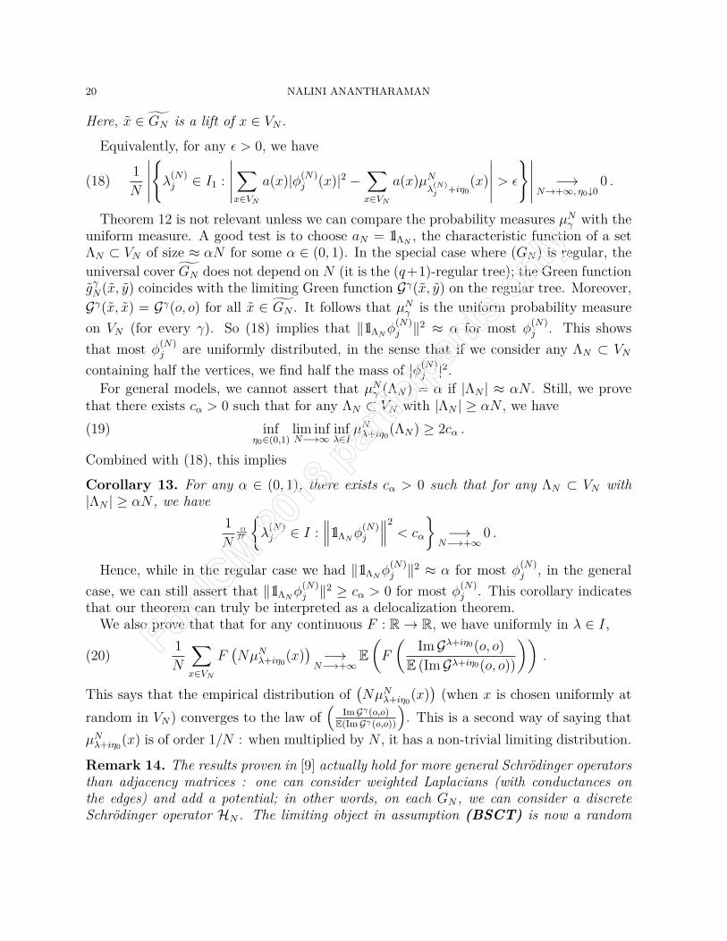
20 NALINI ANANTHARAMAN
Here, x ∈ GN is a lift of x ∈ VN .
Equivalently, for any ϵ > 0, we have
(18) 1
N
∣∣∣∣∣λ(N)j ∈ I1 :
∣∣∣∣∣∑x∈VN
a(x)|ϕ(N)j (x)|2 −
∑x∈VN
a(x)µN
λ(N)j +iη0
(x)
∣∣∣∣∣ > ϵ
∣∣∣∣∣ −→N→+∞, η0↓0
0 .
Theorem 12 is not relevant unless we can compare the probability measures µNγ with the
uniform measure. A good test is to choose aN = 1lΛN, the characteristic function of a set
ΛN ⊂ VN of size ≈ αN for some α ∈ (0, 1). In the special case where (GN) is regular, theuniversal cover GN does not depend on N (it is the (q+1)-regular tree); the Green functiongγN(x, y) coincides with the limiting Green function Gγ(x, y) on the regular tree. Moreover,Gγ(x, x) = Gγ(o, o) for all x ∈ GN . It follows that µN
γ is the uniform probability measureon VN (for every γ). So (18) implies that ∥1lΛN
ϕ(N)j ∥2 ≈ α for most ϕ(N)
j . This showsthat most ϕ(N)
j are uniformly distributed, in the sense that if we consider any ΛN ⊂ VN
containing half the vertices, we find half the mass of |ϕ(N)j |2.
For general models, we cannot assert that µNγ (ΛN) = α if |ΛN | ≈ αN . Still, we prove
that there exists cα > 0 such that for any ΛN ⊂ VN with |ΛN | ≥ αN , we have(19) inf
η0∈(0,1)lim infN−→∞
infλ∈I
µNλ+iη0
(ΛN) ≥ 2cα .
Combined with (18), this implies
Corollary 13. For any α ∈ (0, 1), there exists cα > 0 such that for any ΛN ⊂ VN with|ΛN | ≥ αN , we have
1
N#
λ(N)j ∈ I :
∥∥∥1lΛNϕ(N)j
∥∥∥2 < cα
−→
N−→+∞0 .
Hence, while in the regular case we had ∥1lΛNϕ(N)j ∥2 ≈ α for most ϕ(N)
j , in the generalcase, we can still assert that ∥1lΛN
ϕ(N)j ∥2 ≥ cα > 0 for most ϕ(N)
j . This corollary indicatesthat our theorem can truly be interpreted as a delocalization theorem.
We also prove that that for any continuous F : R → R, we have uniformly in λ ∈ I,
(20) 1
N
∑x∈VN
F(NµN
λ+iη0(x))
−→N−→+∞
E(F
(ImGλ+iη0(o, o)
E (ImGλ+iη0(o, o))
)).
This says that the empirical distribution of(NµN
λ+iη0(x))
(when x is chosen uniformly atrandom in VN) converges to the law of
(ImGγ(o,o)
E(ImGγ(o,o))
). This is a second way of saying that
µNλ+iη0
(x) is of order 1/N : when multiplied by N , it has a non-trivial limiting distribution.
Remark 14. The results proven in [9] actually hold for more general Schrödinger operatorsthan adjacency matrices : one can consider weighted Laplacians (with conductances onthe edges) and add a potential; in other words, on each GN , we can consider a discreteSchrödinger operator HN . The limiting object in assumption (BSCT) is now a random

DELOCALIZATION 21
rooted tree [T , o] endowed with a random Schrödinger operator H. Assumption (Green)has to be modified, replacing the adjacency matrix A by the operator H. Similarly, in thestatement of the theorem, the Green functions gγN to be considered are those of HN liftedto the universal cover GN .
Remark 15. In particular, our result applies to the case where the limiting system ([T , o],H)is T = X (the (q + 1)-regular tree) with an arbitrary origin o, and H = Hϵ = A + ϵWwhere W is a random real-valued potential on X. More precisely the values W(x) (x ∈ X)are i.i.d. random variables of common law ν. This is known as the Anderson model onX. It was shown by A. Klein [76] that the spectrum of Hϵ is a.s. purely absolutely con-tinuous on I = (−2
√q + δ, 2
√q − δ), provided ϵ is small enough (depending on δ). This
just assumes a second moment on ν. Under stronger regularity assumptions on ν, onecan show that Assumption (Green) holds on I (see [11], following Aizenman-Warzel [2]).Examples of sequences of expander regular graphs GN with discrete Schrödinger operatorsHN converging to ([X, o],Hϵ) are given in [10].
Remark 16. Examples of sequences of non-regular graphs satisfying our three assumptionswere investigated in [11]. In the examples considered there, the limiting trees T are treesof finite cone type; roughly speaking, those are trees where the local geometry can only takea finite number of values. If A is the adjacency matrix of such a tree, we showed in [11]that the spectrum σ of A is a finite union of closed intervals, and that there are a finitenumber of points y1, . . . , yℓ in σ such that Assumption (Green) holds on any I of the formσ \ ([y1 − δ, y1 + δ] ∪ . . . ∪ [yℓ − δ, yℓ + δ]) (for any δ > 0). We showed – extending Remark15 – that on such trees, Assumption (Green) remains true after adding a small randompotential to AT . Finally, we showed the existence of sequences (GN) converging to T andsatisfying the (EXP) condition.
4. Perspectives and link with other work
4.1. Random regular graphs. It is important to stress the fact that Theorem 11 holdsfor deterministic sequences of graphs. For any sequence (GN) satisfying the assumptionsof the theorem, the conclusion holds for any observable a. As already noted, the resultonly says something about the delocalization of “most” eigenfunctions, where the “good”eigenfunctions exhibiting delocalization may depend on the choice of the observable a.
In the past years, there has been tremendous interest in spectral statistics and delocal-ization of eigenfunctions of random sequences of graphs and Schrödinger operators. Manypapers consider random regular graphs, with degree going slowly to infinity [113, 45, 15, 13]or fixed [56, 14], sometimes adding a random i.i.d potential [56]. A (labelled) random reg-ular graph on N vertices is produced as follows : given the vertex set 1, . . . , N, considerall the ways to draw edges between those vertices, that produce a (q + 1)-regular graph(without self-loops and multiple edges); note that (q+1)N has to be an even integer. Picka graph at random for the uniform probability measure on all possible configurations.
The very impressive papers [15, 13, 14] show “quantum unique ergodicity” for the adja-cency matrix of random regular graphs : given an observable aN : 1, . . . , N −→ R, for

22 NALINI ANANTHARAMAN
most (q + 1)-regular graphs on the vertices 1, . . . , N we have that∑N
x=1 aN(x)|ϕ(N)j (x)|2
is close to ⟨aN⟩ for all indices j, with an excellent control of the remainder term :Theorem 17 (Bauerschmidt-Huang-Yau [14]). Let ω be such that √q ≥ (ω + 1)22ω+45.
(i) With probability ≥ 1− o(N−ω+8) on the choice of the graph,
∥ϕj∥∞ ≤ (logN)121√N
for all eigenfunctions associated to eigenvalues such that |λj ± 2√q| > (logN)−3/2.
(ii) (Quantum Unique Ergodicity for random regular graphs) Given an observable aN :1, . . . , N −→ R, we have, with probability ≥ 1 − o(N−ω+8) on the choice of the graph,for N large enough,
(21)
∣∣∣∣∣N∑
x=1
aN(x)|ϕ(N)j (x)|2 − ⟨aN⟩
∣∣∣∣∣ ≤ (logN)250
N
√∑x
|aN(x)|2,
for all eigenfunctions associated to eigenvalues λj ∈ (−2√q+ϵ, 2
√q−ϵ) (bulk eigenvalues).
In particular, if aN = 1lΛNwhere ΛN ⊂ 1, . . . , N, we find∣∣∣∣∣∑
x∈ΛN
|ϕ(N)j (x)|2 − |ΛN |
N
∣∣∣∣∣ ≤ (logN)250
N
√|ΛN |.
(Note in passing that ω > 8 implies that q > 2128).So the ℓ∞-norm of bulk eigenfunctions is as small as can be, and QUE takes place on
sets of size |ΛN | > (logN)500. By comparison, in Theorem 11, for graphs whose girth goesto ∞, our proof would never do better than∣∣∣∣∣∑
x∈ΛN
|ϕ(N)j (x)|2 − |ΛN |
N
∣∣∣∣∣ ≤ 1√N logN
√|ΛN |.
So Theorem 17 is a considerable strengthening of (18), that only said something formost indices j and for |ΛN | > N1/2. This possibility to prove QUE is, of course, due to thefact that aN is probabilistically independent of the choice of the graph; in Theorem 11 and(18), aN could depend on the graph. It might well be that a positive proportion of graphscontradicts QUE, if we were allowed to choose observables aN depending on the graph (thisis a completely open question). Note also that if we are given a deterministic sequence ofregular graphs (for instance, say, the Lubotzky-Phillips-Sarnak Ramanujan graphs [86]),we do not know if Theorem 17 applies to it, as it is an almost sure conclusion.Remark 18. Note that we emphasized Theorem 17 from [14] because our main concernhere is the delocalization of eigenfunctions. The main focus of [14] is however on theuniversality of the local spectral statistics for random regular graphs. This would deserve aseparate paper.
The recent paper by Backhausz and Szegedy [12] proves a very important result, sayingthat for almost all random regular graphs GN on N vertices, and all eigenvectors ϕ(N)
j s,

DELOCALIZATION 23
the value distribution of√Nϕj(x) as x runs over 1, . . . , N is close to some Gaussian
N (0, σ2j ) with 0 ≤ σj ≤ 1. More generally, for any R ≥ 0, picking x uniformly at random
in 1, . . . , N and looking at the values of (√Nϕj(y))y,d(y,x)≤R in the vicinity of x in GN ,
the obtained random function is close in distribution to a gaussian process on BX(o,R).The covariance function has to be of the form σ2
jΦλj(d(x, y)) where Φλj
is the sphericalfunction of parameter λj on the (q + 1)-regular tree X. Proving that σj = 1, or even justthat σj = 0, is a challenge; it would amount to proving that eigenfunctions cannot belocalized on o(N) vertices. Theorem 10 does not say this, it only says that eigenfunctionscannot be localized on Nα vertices. Our Theorem 11, or the random version Theorem 17do not say this either, because we can only test one observable aN at a time. The indicesj for which (18) holds, or the set of graphs satisfying (21), depend on aN . If we wanted tohave a common set that does the job for all observables (whose number is exponential inN), we would need to have exponential error bounds in (18) or (21).
4.2. From graph Laplacians to Hecke operators. What do these discrete results teachus about the problem we were originally interested in, namely the eigenfunctions of theLaplace-Beltrami operators on a riemannian manifold ? A natural question that comesto mind is to try to adapt Theorem 11 to sequences of graphs that are finer and finertriangulations of some given Riemann surface. With the appropriate choice of conductanceson the edges, the corresponding discrete Laplacians approximate the continuous Laplacian.At the present time, we are unable to say anything about such graphs, because they havemany loops and this is excluded by the hypotheses of Theorem 11.
But let us throw a look in a different direction, that of “Arithmetic quantum ergodicity”.Consider S2, the 2-dimensional sphere with its usual, round metric. The eigenfunctions
of ∆S2 are spherical harmonics, i.e. restrictions to S2 ⊂ R3 of harmonic homogeneouspolynomials in 3 variables. Harmonic homogeneous polynomials of degree ℓ give rise toeigenfunctions of ∆S2 for the eigenvalue −ℓ(ℓ+1) (the dimension of the eigenspace is 2ℓ+1).
The Laplacian ∆S2 commutes with the infinitesimal rotation J12 = 1i
(x2
∂∂x2
− x2∂
∂x1
).
Note that J12 is a differential operator of order 1, and that its principal symbol is thekinetic momentum around the vertical axis.
The basis (ϕn) = (Y mℓ )ℓ≥0,|m|≤ℓ of joint eigenfunctions of ∆Sd and J12 cannot satisfy the
conclusions of Theorem 5. In fact, using the same notation as in §2.4, let us considera subsequence (ϕnk
) such that ⟨ϕnk, Aϕnk
⟩ converges for all A; the limit is of the form∫S∗M
σ0(A)dµ, where µ is a probability measure on S∗M . The fact that ϕnkis an eigen-
function of J12 is converted into the property that µ is carried by a level set of the kineticmomentum (which is a submanifold of positive codimension in S∗M); thus µ cannot bethe Lebesgue measure.
Because the spectrum of the Laplacian has huge multiplicities, one can wonder whetherother bases of eigenfunctions on the sphere satisfy Theorem 5. Zelditch had the idea ofconsidering random eigenbases [118]. He showed that “almost every” choice of eigenbasissatisfies Theorem 5 (this was strengthened to Quantum Unique Ergodicity by Van DerKam [114]).

24 NALINI ANANTHARAMAN
Brooks, Le Masson and Lindenstrauss [37] showed quantum ergodicity for an explicitbasis of eigenfunctions of ∆S2 , that are also eigenfunctions of a kind of “discrete” Laplacianon S2 : for g1, . . . , gk a finite set of rotations in SO(3),
Tkf(x) =k∑
j=1
(f(gjx) + f(g−1j x))
commutes with ∆S2 .
Theorem 19 (Brooks, Le Masson and Lindenstrauss [37]). Assume that g1, . . . , gk generatea free subgroup of SO(3).
For each ℓ, let (ψ(ℓ)j )2ℓ+1
j=1 be an orthonormal family of eigenfunctions of −∆S2 of eigen-value ℓ(ℓ+ 1), that are also eigenfunctions of Tk.
Then for any continuous function a on S2, we have
1
2ℓ+ 1
2ℓ+1∑j=1
∣∣∣∣∫M
a(x)|ψ(ℓ)j (x)|2dVol(x)−
∫M
a(x)dVol(x)
∣∣∣∣2 −→ℓ−→∞
0.
Restricting Tk to the space of spherical harmonics of degree ℓ is shown to be roughly thesame as letting Tk act on a discretization of the sphere by an ℓ−1-net. This is the sameas studying the Laplacian on a 2k-regular graph with N ∼ ℓ2 vertices, and if g1, . . . , gkgenerate a free subgroup, this graph has few short loops. Thus, Theorem 19 is similar toTheorem 11. The theorem on regular graphs can serve as a canvas to prove Theorem 19.
Remark 20. Tk is not a pseudodifferential operator, so the argument sketched above toshow that the basis (Y m
ℓ )ℓ≥0,|m|≤ℓ could not satisfy quantum ergodicity does not apply here.
Remark 21. We note that for very special choices of rotations – rotations that correspondto norm n elements in an order in a quaternion division algebra, the operators Tk are calledHecke operators. It has been conjectured by Böcherer, Sarnak, and Schulze-Pillot [25] thatsuch joint eigenfunctions satisfy the much stronger quantum unique ergodicity property.This conjecture is still open.
The idea of adapting a result on discrete graphs to the realm of Hecke operators onarithmetic manifolds had already been used in [39]. In 2000, Bourgain and Lindenstrausshad considered the measures µ obtained in Theorem 7, when the eigenfunctions (ϕn) arejoint eigenfunctions of ∆ and of the infinite family of Hecke operators on an arithmetichyperbolic surface (e.g., the modular surface). They were able to show that µ has positiveentropy on almost-every ergodic component, and this fact was a key ingredient in the proofof Arithmetic Quantum Unique Ergodicity by Lindenstrauss [84]. In [39], Brooks andLindenstrauss used the fact that a Hecke operator, restricted to a net in the manifold M ,acts similarly to the discrete Laplacian on a regular graph with few short loops, to adaptTheorem 10 and show that µ has positive entropy on almost-every ergodic component,using only one Hecke operator.

DELOCALIZATION 25
In the next paragraph, we mention another continuous adaptation of Theorem 11 :instead of thinking of discrete Laplacians living in a riemannian manifold and restrictedto a finer and finer net, we look at riemannian manifolds that get larger and larger :
4.3. Quantum ergodicity on Riemann surfaces of high genus. Theorems 11 and 12were dubbed as “quantum ergodicity” theorems in reference to the historical Theorem 5.However, we already noted a difference in the meaning of these results. Theorem 5 holds inthe high-frequency régime, whereas the graph-results deal with the large-scale régime. So,a continuous analogue of Theorem 11 would be to consider compact Riemannian manifoldswhose volume goes to infinity. Such a result was obtained by Le Masson and Sahlsten forRiemann surfaces of high genus :
Theorem 22 (Le Masson– Sahlsten [80]). Let (SN) be a sequence of hyperbolic surfaces,whose genus (equivalently, volume) goes to ∞.
(EXP) Assume the first eigenvalue λ1(N) of −∆ on SN is bounded away from 0 asN −→ ∞.
(BSH)Assume there are few short geodesics; in other words, (SN) converges in theBenjamini-Schramm sense to the hyperbolic disc : for any R > 0,
limN−→+∞
Volx ∈ SN , ρ(x) < RVol(SN)
= 0
where ρ(x) means the injectivity radius at x.Fix an interval I ⊂ (1/4,+∞).Let (ϕ(N)
i ) be an orthonormal basis of eigenfunctions of the Laplacian on SN .Let a = aN : SN −→ C be such that |a(x)| ≤ 1 for all x ∈ SN . Then
limN−→+∞
1
V ol(SN)
∑λi(N)∈I
∣∣∣∣∫SN
a(x)|ϕ(N)i (x)|2dx− ⟨a⟩
∣∣∣∣2 = 0
where ⟨a⟩ = 1V ol(SN )
∫SNa(x)dx.
We note that (1/4,+∞) is the L2-spectrum of the Laplacian on the hyperbolic disc. Thisspectrum is purely absolutely continuous. So, like in the graph case, we are working withthe sequence of compact SN converging to an infinite-volume simply connected manifold,with purely absolutely continuous spectrum. It would be interesting to find more examplesof such manifolds (and to extend Theorem 22 to that more general setting), but we havealready mentioned in §2.5.1 the difficulty of proving absolutely continuous spectrum.
A tremendously interesting question would to put this result in the framework of randomRiemann surfaces :
• does Quantum Unique Ergodicity hold for large random Riemann surfaces, in thespirit of Theorem 17 ?
• for a typical random Riemann surface, is the value distribution of the eigenfunc-tions (ϕ(N)
i ) asymptotically gaussian, similarly to the case of random regular graphsrecently treated by Backhausz-Szegedy in [12] ? This would come very close to

26 NALINI ANANTHARAMAN
justifying Berry’s Random Wave ansatz [20] – the latter was formulated in thehigh-frequency régime, but a version in the large-scale limit would also be of highinterest.
The most natural notion of random Riemann surface of genus g is obtained by putting theWeil-Petersson volume measure on their moduli spaces. The volume of the moduli spaceof Riemann surface of genus g was computed by Mirzakhani (see [91, 92] and referencestherein), and she could give its asymptotic behaviour as g −→ +∞. She showed that arandom Riemann surface has a uniform spectral gap in the spectrum of the Laplacian, asg −→ +∞; this is similar to what is known for random regular graphs. She also obtainedasymptotic information about the law of the length of the shortest closed geodesic and theshortest separating geodesic. However, this model of random Riemann surfaces does notseem flexible enough to allow for a direct transposition of the wonderful result of [12]. Thisis a very intriguing topic to explore.
References[1] De Luca A., Altshuler B., Kravtsov V. E., and Scardicchio A. Anderson localization on the bethe
lattice: Nonergodicity of extended states. Phys. Rev. Lett., 113, 2014.[2] Michael Aizenman and Simone Warzel. Absolutely continuous spectrum implies ballistic transport
for quantum particles in a random potential on tree graphs. J. Math. Phys., 53(9):095205, 15, 2012.[3] Nalini Anantharaman. Entropy and the localization of eigenfunctions. Ann. of Math. (2), 168(2):435–
475, 2008.[4] Nalini Anantharaman. Quantum ergodicity on regular graphs. Comm. Math. Phys., 353(2):633–690,
2017.[5] Nalini Anantharaman and Etienne Le Masson. Quantum ergodicity on large regular graphs. Duke
Math. J., 164(4):723–765, 2015.[6] Nalini Anantharaman and Stéphane Nonnenmacher. Entropy of semiclassical measures of the Walsh-
quantized baker’s map. Ann. Henri Poincaré, 8(1):37–74, 2007.[7] Nalini Anantharaman and Stéphane Nonnenmacher. Half-delocalization of eigenfunctions for the
Laplacian on an Anosov manifold. Ann. Inst. Fourier (Grenoble), 57(7):2465–2523, 2007. FestivalYves Colin de Verdière.
[8] Nalini Anantharaman and Mostafa Sabri. Poisson kernel expansions for schrödinger operators ontrees. preprint, https://arxiv.org/abs/1610.05907, 2016.
[9] Nalini Anantharaman and Mostafa Sabri. Quantum ergodicity : from spectral to spatial delocaliza-tion arxiv:1704.02766. preprint, 2017.
[10] Nalini Anantharaman and Mostafa Sabri. Quantum ergodicity for the Anderson model on regulargraphs. J. Math. Phys., 58(9):091901, 10, 2017.
[11] Nalini Anantharaman and Mostafa Sabri. Recent results of quantum ergodicity on graphs and furtherinvestigation. preprint, arXiv:1711.07666, 2017.
[12] Agnes Backhausz and Balazs Szegedy. On the almost eigenvectors of random regular graphsarxiv:1607.04785. preprint, 2016.
[13] Roland Bauerschmidt, Jiaoyang Huang, Antti Knowles, and Horng-Tzer Yau. Bulk eigenvalue sta-tistics for random regular graphs arxiv:1505.06700. 2015.
[14] Roland Bauerschmidt, Jiaoyang Huang, and Horng-Tzer Yau. Local kesten–mckay law for randomregular graphs arxiv:1609.09052. 2016.
[15] Roland Bauerschmidt, Antti Knowles, and Horng-Tzer Yau. Local semicircle law for random regulargraphs. Comm. Pure Appl. Math., 70(10):1898–1960, 2017.

DELOCALIZATION 27
[16] Itai Benjamini and Oded Schramm. Recurrence of distributional limits of finite planar graphs. Elec-tron. J. Probab., 6:no. 23, 13, 2001.
[17] Pierre H. Bérard. On the wave equation on a compact Riemannian manifold without conjugatepoints. Math. Z., 155(3):249–276, 1977.
[18] G. Berkolaiko, J. P. Keating, and U. Smilansky. Quantum ergodicity for graphs related to intervalmaps. Comm. Math. Phys., 273(1):137–159, 2007.
[19] G. Berkolaiko, J. P. Keating, and B. Winn. No quantum ergodicity for star graphs. Comm. Math.Phys., 250(2):259–285, 2004.
[20] Michael Berry. Regular and irregular semiclassical wavefunctions. J. Phys. A, 10(12):2083–2091,1977.
[21] Michael Berry and Michael Tabor. Level clustering in the regular spectrum. Proc. Royal Soc. A,pages 375–394, 1977.
[22] Matthew Blair and Christopher Sogge. Concerning toponogov’s theorem and logarithmic improve-ment of estimates of eigenfunctions, to appear in j. diff. geom. 2015.
[23] Matthew Blair and Christopher Sogge. Logarithmic improvements in lp bounds for eigenfunctions atthe critical exponent in the presence of nonpositive curvature. 2017.
[24] Matthew D. Blair and Christopher D. Sogge. Refined and Microlocal Kakeya–Nikodym Bounds ofEigenfunctions in Higher Dimensions. Comm. Math. Phys., 356(2):501–533, 2017.
[25] Siegfried Böcherer, Peter Sarnak, and Rainer Schulze-Pillot. Arithmetic and equidistribution of mea-sures on the sphere. Comm. Math. Phys., 242(1-2):67–80, 2003.
[26] O. Bohigas, M.-J. Giannoni, and C. Schmit. Characterization of chaotic quantum spectra and uni-versality of level fluctuation laws. Phys. Rev. Lett., 52(1):1–4, 1984.
[27] Oriol Bohigas. Random matrix theories and chaotic dynamics. In Chaos et physique quantique (LesHouches, 1989), pages 87–199. North-Holland, Amsterdam, 1991.
[28] Niels Bohr. On the constitution of atoms and molecules. Philosophical Magazine, 26:1–24, 1913.[29] Jens Bolte and Rainer Glaser. A semiclassical Egorov theorem and quantum ergodicity for matrix
valued operators. Comm. Math. Phys., 247(2):391–419, 2004.[30] Yannick Bonthonneau. The Θ function and the Weyl law on manifolds without conjugate points.
Doc. Math., 22:1275–1283, 2017.[31] Yannick Bonthonneau and Steve Zelditch. Quantum ergodicity for Eisenstein functions. C. R. Math.
Acad. Sci. Paris, 354(9):907–911, 2016.[32] David Borthwick. Spectral theory of infinite-area hyperbolic surfaces, volume 256 of Progress in Math-
ematics. Birkhäuser Boston, Inc., Boston, MA, 2007.[33] P. Bourgade and H.-T. Yau. The eigenvector moment flow and local quantum unique ergodicity.
preprint, 2013.[34] Jean Bourgain and Elon Lindenstrauss. Entropy of quantum limits. Comm. Math. Phys., 233(1):153–
171, 2003.[35] Louis Brillouin. La mécanique ondulatoire de schrödinger; une méthode générale de résolution par
approximations successives. C. R. A. S., (183):24–26, 1926.[36] Shimon Brooks and Étienne Le Masson. lp-norms of eigenfunctions on regular graphs and on the
sphere arxiv:1710.10922 d. preprint, 2017.[37] Shimon Brooks, Étienne Le Masson, and Elon Lindenstrauss. Quantum ergodicity and averaging
operators on the sphere. Int. Math. Res. Not., 2015. To appear, arXiv:1505.03887.[38] Shimon Brooks and Elon Lindenstrauss. Non-localization of eigenfunctions on large regular graphs.
Israel J. Math., 193(1):1–14, 2013.[39] Shimon Brooks and Elon Lindenstrauss. Joint quasimodes, positive entropy, and quantum unique
ergodicity. Invent. Math., 198(1):219–259, 2014.[40] Y. Colin de Verdière. Ergodicité et fonctions propres du laplacien. Comm. Math. Phys., 102(3):497–
502, 1985.

28 NALINI ANANTHARAMAN
[41] Y. Colin de Verdière. Semi-classical measures on quantum graphs and the gauss map of the deter-minant manifold. Ann. H. Poincaré, to appear, 2013.
[42] Yves Colin de Verdière, Luc Hillairet, and Emmanuel Trélat. Spectral asymptotics for sub-riemannianlaplacians. i: quantum ergodicity and quantum limits in the 3d contact case. preprint, 2015.
[43] Dominique Delande. Chaos in atomic and molecular physics. In Chaos et physique quantique (LesHouches, 1989), pages 665–726. North-Holland, Amsterdam, 1991.
[44] Persi Diaconis and Daniel Stroock. Geometric bounds for eigenvalues of Markov chains. Ann. Appl.Probab., 1(1):36–61, 1991.
[45] Ioana Dumitriu and Soumik Pal. Sparse regular random graphs: spectral density and eigenvectors.Ann. Probab., 40(5):2197–2235, 2012.
[46] Semyon Dyatlov and Colin Guillarmou. Microlocal limits of plane waves and Eisenstein functions.Ann. Sci. Éc. Norm. Supér. (4), 47(2):371–448, 2014.
[47] Semyon Dyatlov and Long Jin. Semiclassical measures on hyperbolic surfaces have full supportarxiv:1705.05019. preprint, 2017.
[48] Manfred Einsiedler and Elon Lindenstrauss. Diagonalizable flows on locally homogeneous spaces andnumber theory. In International Congress of Mathematicians. Vol. II, pages 1731–1759. Eur. Math.Soc., Zürich, 2006.
[49] Albert Einstein. über einen die erzeugung und verwandlung des lichts betreffenden heuristischengesichtspunkt. Annalen der Physik, 17, 1905.
[50] Albert Einstein. Zum quantensatz von sommerfeld und epstein. Verhandl. deut. physik. Ges., 1917.[51] László Erd˝ os, Antti Knowles, Horng-Tzer Yau, and Jun Yin. Spectral statistics of Erdös-Rényi
graphs I: Local semicircle law. Ann. Probab., 41(3B):2279–2375, 2013.[52] László Erdős, Benjamin Schlein, and Horng-Tzer Yau. Local semicircle law and complete delocaliza-
tion for Wigner random matrices. Comm. Math. Phys., 287(2):641–655, 2009.[53] László Erdős, Benjamin Schlein, and Horng-Tzer Yau. Semicircle law on short scales and delocaliza-
tion of eigenvectors for Wigner random matrices. Ann. Probab., 37(3):815–852, 2009.[54] Frédéric Faure and Stéphane Nonnenmacher. On the maximal scarring for quantum cat map eigen-
states. Comm. Math. Phys., 245(1):201–214, 2004.[55] Frédéric Faure, Stéphane Nonnenmacher, and Stephan De Bièvre. Scarred eigenstates for quantum
cat maps of minimal periods. Comm. Math. Phys., 239(3):449–492, 2003.[56] Leander Geisinger. Convergence of the density of states and delocalization of eigenvectors on random
regular graphs. J. Spectr. Theory, 5(4):783–827, 2015.[57] Patrick Gérard and Éric Leichtnam. Ergodic properties of eigenfunctions for the Dirichlet problem.
Duke Math. J., 71(2):559–607, 1993.[58] S. Gnutzmann, J. P. Keating, and F. Piotet. Eigenfunction statistics on quantum graphs. Ann.
Physics, 325(12):2595–2640, 2010.[59] Colin Guillarmou and Frédéric Naud. Equidistribution of Eisenstein series on convex co-compact
hyperbolic manifolds. Amer. J. Math., 136(2):445–479, 2014.[60] Xiaolong Han. Small scale quantum ergodicity in negatively curved manifolds. Nonlinearity,
28(9):3263–3288, 2015.[61] Xiaolong Han. Small scale equidistribution of random eigenbases. Comm. Math. Phys., 349(1):425–
440, 2017.[62] Andrew Hassell. Ergodic billiards that are not quantum unique ergodic. Ann. of Math. (2),
171(1):605–619, 2010. With an appendix by the author and Luc Hillairet.[63] Andrew Hassell and Melissa Tacy. Improvement of eigenfunction estimates on manifolds of nonpos-
itive curvature. Forum Math., 27(3):1435–1451, 2015.[64] Werner Heisenberg. über quantentheoretische umdeutung kinematischer und mechanischer beziehun-
gen. Zeitschrift f. Physik, 33:879–893, 1925.

DELOCALIZATION 29
[65] B. Helffer, A. Martinez, and D. Robert. Ergodicité et limite semi-classique. Comm. Math. Phys.,109(2):313–326, 1987.
[66] Eric Heller. Wavepacket dynamics and quantum chaology. In Chaos et physique quantique (LesHouches, 1989), pages 549–661. North-Holland, Amsterdam, 1991.
[67] Hamid Hezari and Gabriel Rivière. Lp norms, nodal sets, and quantum ergodicity. Adv. Math.,290:938–966, 2016.
[68] Maxime Ingremeau. Distorted plane waves on manifolds of nonpositive curvature. Comm. Math.Phys., 350(2):845–891, 2017.
[69] Dmitry Jakobson. Quantum unique ergodicity for Eisenstein series on PSL2(Z)\PSL2(R). Ann. Inst.Fourier (Grenoble), 44(5):1477–1504, 1994.
[70] Dmitry Jakobson, Yuri Safarov, and Alexander Strohmaier. The semiclassical theory of discontinuoussystems and ray-splitting billiards. Amer. J. Math., 137(4):859–906, 2015. With an appendix by YvesColin de Verdière.
[71] Dmitry Jakobson and Alexander Strohmaier. High energy limits of Laplace-type and Dirac-typeeigenfunctions and frame flows. Comm. Math. Phys., 270(3):813–833, 2007.
[72] Dmitry Jakobson, Alexander Strohmaier, and Steve Zelditch. On the spectrum of geometric operatorson Kähler manifolds. J. Mod. Dyn., 2(4):701–718, 2008.
[73] J. P. Keating. Quantum graphs and quantum chaos. In Analysis on graphs and its applications,volume 77 of Proc. Sympos. Pure Math., pages 279–290. Amer. Math. Soc., Providence, RI, 2008.
[74] J. P. Keating, J. Marklof, and B. Winn. Value distribution of the eigenfunctions and spectral deter-minants of quantum star graphs. Comm. Math. Phys., 241(2-3):421–452, 2003.
[75] Harry Kesten. Symmetric random walks on groups. Trans. Amer. Math. Soc., 92:336–354, 1959.[76] Abel Klein. Extended states in the Anderson model on the Bethe lattice. Adv. Math., 133(1):163–184,
1998.[77] Tsampikos Kottos and Uzy Smilansky. Quantum chaos on graphs. Phys. Rev. Lett., 79:4794–7, 1997.[78] Tsampikos Kottos and Uzy Smilansky. Periodic orbit theory and spectral statistics for quantum
graphs. Ann. Physics, 274(1):76–124, 1999.[79] Hendrik Anthony Kramers. Wellenmechanik und halbzahlige quantisierung. Zeitschrift f. Physik,
(39):828–840, 1926.[80] Étienne Le Masson and Tuomas Sahlsten. Quantum ergodicity and benjamini-schramm convergence
of hyperbolic surfaces. arxiv:1605.05720. Duke Math. J., to appear.[81] F. Ledrappier and L.-S. Young. The metric entropy of diffeomorphisms. I. Characterization of mea-
sures satisfying Pesin’s entropy formula. Ann. of Math. (2), 122(3):509–539, 1985.[82] F. Ledrappier and L.-S. Young. The metric entropy of diffeomorphisms. II. Relations between entropy,
exponents and dimension. Ann. of Math. (2), 122(3):540–574, 1985.[83] Stephen Lester and Zeév Rudnick. Small scale equidistribution of eigenfunctions on the torus. Comm.
Math. Phys., 350(1):279–300, 2017.[84] Elon Lindenstrauss. Invariant measures and arithmetic quantum unique ergodicity. Ann. of Math.
(2), 163(1):165–219, 2006.[85] Elon Lindenstrauss. Equidistribution in homogeneous spaces and number theory. In Proceedings of
the International Congress of Mathematicians. Volume I, pages 531–557. Hindustan Book Agency,New Delhi, 2010.
[86] A. Lubotzky, R. Phillips, and P. Sarnak. Ramanujan graphs. Combinatorica, 8(3):261–277, 1988.[87] W. Luo and P. Sarnak. Number variance for arithmetic hyperbolic surfaces. Comm. Math. Phys.,
161(2):419–432, 1994.[88] Jens Marklof. Pair correlation densities of inhomogeneous quadratic forms. Ann. of Math. (2),
158(2):419–471, 2003.[89] Brendan D. McKay. The expected eigenvalue distribution of a large regular graph. Linear Algebra
Appl., 40:203–216, 1981.

30 NALINI ANANTHARAMAN
[90] Brendan D. McKay, Nicholas C. Wormald, and Beata Wysocka. Short cycles in random regulargraphs. Electron. J. Combin., 11(1):Research Paper 66, 12 pp. (electronic), 2004.
[91] Maryam Mirzakhani. On Weil-Petersson volumes and geometry of random hyperbolic surfaces. InProceedings of the International Congress of Mathematicians. Volume II, pages 1126–1145. Hindus-tan Book Agency, New Delhi, 2010.
[92] Maryam Mirzakhani. Growth of Weil-Petersson volumes and random hyperbolic surfaces of largegenus. J. Differential Geom., 94(2):267–300, 2013.
[93] Max Planck. über eine verbesserung der wienschen spektralgleichung. Verhandl. deut. physik. Ges.,13:202–204, 1900.
[94] Gabriel Rivière. Entropy of semiclassical measures in dimension 2. Duke. Math. J., 155(2):271–335,2010.
[95] Zeév Rudnick and Peter Sarnak. The behaviour of eigenstates of arithmetic hyperbolic manifolds.Comm. Math. Phys., 161(1):195–213, 1994.
[96] Peter Sarnak. Arithmetic quantum chaos. In The Schur lectures (1992) (Tel Aviv), volume 8 of IsraelMath. Conf. Proc., pages 183–236. Bar-Ilan Univ., Ramat Gan, 1995.
[97] Peter Sarnak. Values at integers of binary quadratic forms. In Harmonic analysis and number theory(Montreal, PQ, 1996), volume 21 of CMS Conf. Proc., pages 181–203. Amer. Math. Soc., Providence,RI, 1997.
[98] Peter Sarnak. Spectra of hyperbolic surfaces. Bull. Amer. Math. Soc. (N.S.), 40(4):441–478, 2003.[99] Erwin Schrödinger. Quantisierung als eigenwertproblem (erste mitteilung). Annalen der Physik (4),
79:361–376, 1926.[100] Erwin Schrödinger. Quantisierung als eigenwertproblem (zweite mitteilung). Annalen der Physik (4),
79:489–527, 1926.[101] Erwin Schrödinger. über das verhältnis der heisenberg–born–jordanschen quantenmechanik zu der
meinen. Annalen der Physik (4), 79:734–756, 1926.[102] Atle Selberg. Remarks on the distribution of poles of Eisenstein series. In Festschrift in honor of I.
I. Piatetski-Shapiro on the occasion of his sixtieth birthday, Part II (Ramat Aviv, 1989), volume 3of Israel Math. Conf. Proc., pages 251–278. Weizmann, Jerusalem, 1990.
[103] Martin Sieber and Klaus Richter. Correlations between periodic orbits and their rôle in spectralstatistics. Physica Scripta, T90, 2001.
[104] Uzy Smilansky. Quantum chaos on discrete graphs. J. Phys. A, 40(27):F621–F630, 2007.[105] Uzy Smilansky. Discrete graphs – a paradigm model for quantum chaos. Séminaire Poincaré, XIV:1–
26, 2010.[106] A. I. Šnirel′man. Ergodic properties of eigenfunctions. Uspehi Mat. Nauk, 29(6(180)):181–182, 1974.[107] Christopher D. Sogge. Concerning the Lp norm of spectral clusters for second-order elliptic operators
on compact manifolds. J. Funct. Anal., 77(1):123–138, 1988.[108] Christopher D. Sogge and Steve Zelditch. Riemannian manifolds with maximal eigenfunction growth.
Duke Math. J., 114(3):387–437, 2002.[109] Christopher D. Sogge and Steve Zelditch. Focal points and sup-norms of eigenfunctions. Rev. Mat.
Iberoam., 32(3):971–994, 2016.[110] Christopher D. Sogge and Steve Zelditch. Focal points and sup-norms of eigenfunctions II: the two-
dimensional case. Rev. Mat. Iberoam., 32(3):995–999, 2016.[111] K. Soundararajan. Quantum unique ergodicity and number theory. In Proceedings of the International
Congress of Mathematicians. Volume II, pages 357–382. Hindustan Book Agency, New Delhi, 2010.[112] Kannan Soundararajan. Quantum unique ergodicity for SL2(Z)\H. Ann. of Math. (2), 172(2):1529–
1538, 2010.[113] Linh V. Tran, Van H. Vu, and Ke Wang. Sparse random graphs: eigenvalues and eigenvectors.
Random Structures Algorithms, 42(1):110–134, 2013.[114] Jeffrey M. VanderKam. L∞ norms and quantum ergodicity on the sphere. Internat. Math. Res.
Notices, (7):329–347, 1997.
DELOCALIZATION 31
[115] Gregor Wentzel. Eine verallgemeinerung der quantenbedingungen für die zwecke der wellenmechanik.Zeitschrift f. Physik, (38):518–529, 1926.
[116] Steven Zelditch. Uniform distribution of eigenfunctions on compact hyperbolic surfaces. Duke Math.J., 55(4):919–941, 1987.
[117] Steven Zelditch. Mean Lindelöf hypothesis and equidistribution of cusp forms and Eisenstein series.J. Funct. Anal., 97(1):1–49, 1991.
[118] Steven Zelditch. Quantum ergodicity on the sphere. Comm. Math. Phys., 146(1):61–71, 1992.[119] Steven Zelditch and Maciej Zworski. Ergodicity of eigenfunctions for ergodic billiards. Comm. Math.
Phys., 175(3):673–682, 1996.
IRMA, 7 rue René-Descartes, 67084 STRASBOURG CEDEX, FRANCEE-mail address: [email protected]