Embed Size (px)
Citation preview

Probab. Theory Relat. Fields (2017) 167:673–776DOI 10.1007/s00440-015-0692-y
Delocalization for a class of random block bandmatrices
Zhigang Bao1 · László Erdos1
Received: 7 April 2015 / Revised: 11 November 2015 / Published online: 23 January 2016© The Author(s) 2016. This article is published with open access at Springerlink.com
Abstract We consider N × N Hermitian random matrices H consisting of blocks ofsize M ≥ N 6/7. The matrix elements are i.i.d. within the blocks, close to a Gaussianin the four moment matching sense, but their distribution varies from block to block toform a block-band structure, with an essential band width M . We show that the entriesof theGreen’s functionG(z) = (H−z)−1 satisfy the local semicircle lawwith spectralparameter z = E + iη down to the real axis for any η � N−1, using a combinationof the supersymmetry method inspired by Shcherbina (J Stat Phys 155(3): 466–499,2014) and the Green’s function comparison strategy. Previous estimates were validonly for η � M−1. The new estimate also implies that the eigenvectors in the middleof the spectrum are fully delocalized.
Keywords Random band matrix · Supersymmetry · Green’s function comparison ·Local semicircle law · Delocalization
Mathematics Subject Classification 15B52 · 81Q60 · 82B44
Z. Bao was supported by ERC Advanced Grant RANMAT No. 338804; L. Erdos was partially supportedby ERC Advanced Grant RANMAT No. 338804.
B László [email protected]
Zhigang [email protected]
1 IST Austria, Am Campus 1, 3400 Klosterneuberg, Austria
123

674 Z. Bao, L. Erdos
1 Introduction
Grassmann integration with supersymmetric (SUSY) methods is ubiquitous in thephysics literature of random quantum systems, see e.g. the basic monograph of Efetov[7]. This approach is especially effective for analyzing the Green function in the mid-dle of the bulk spectrum with spectral parameter close to the real axis, i.e. precisely inthe regime where other methods often fail. The main algebraic strength lies in the factthat Gaussian integrals with Grassmann variables counterbalance the determinantsobtained in the partition functions of complex Gaussian integrals. This greatly sim-plifies algebraic manipulations as it was demonstrated in several papers, see e.g. theproof of the absolutely continuous spectrum on the Bethe lattice by Klein [17] or thebounds on the Lyapunov exponents for random walks in random environment at thecritical energy byWang [29]. However, in theoretical physics Grassmann integrationsare also commonly used as an analytic tool by performing saddle point analysis onthe superspace coordinatized by complex and Grassmann variables. Since Grassmannvariables lack the concept of size, the rigorous justification of this very appealing ideais notoriously difficult.
Initiated by Spencer (see [26] for a summary) and starting with the paper [4] byDisertori, Pinson and Spencer, only a handful of mathematical papers have succeededin exploiting this powerful tool in an essentially analytic way. We still lack the mathe-matical framework of a full-fledged analysis on the superspace that would enable us totranslate physics arguments into proofs directly, but a combination of refined algebraicidentities from physics (such as the superbosonization formula) and a careful analysishave yielded results that are currently inaccessible with more standard probabilisticmethods. In this paper we present such results on random band matrices that surpass awell known limitation of the recently developed probabilistic techniques to prove thelocal versions of the celebrated Wigner semicircle law. We start with introducing thephysical motivation of our model.
The Hamiltonian of quantum systems on a graph with vertex set Γ is a self-adjointmatrix H = (hab)a,b∈Γ , H = H∗. The matrix elements hab represent the quantumtransition rates from vertex a to b. Disordered quantum systems have random matrixelements. We assume they are centered, Ehab = 0, and independent subject to thebasic symmetry constraint hab = hba . The variance σ 2ab := E|hab|2 represents thestrength of the transition from a to b and we use a scaling where the norm ‖H‖ istypically order 1. The simplest case is the mean field model, where hab are identicallydistributed; this is the standard Wigner matrix ensemble [31]. The other prominentexample is the Anderson model [2] or random Schrödinger operator, H = Δ + V ,where the kinetic energy Δ is the (deterministic) graph Laplacian and the potentialV = (Vx )x∈Γ is an on-site multiplication operator with random multipliers. If Γ is adiscrete d-dimensional torus then only few matrix elements hab are nonzero and theyconnect nearest neighbor points in the torus, dist(a, b) ≤ 1. This is in sharp contrastto the mean field character of the Wigner matrices.
Random band matrices naturally interpolate between the mean field Wigner matri-ces and the short range Anderson model. They are characterized by a parameter M ,called the band width, such that the matrix elements hab for dist(a, b) ≥ M are zero
123

Delocalization for a class of random block band matrices 675
or negligible. If M is comparable with the diameter L of the system then we are in themean field regime, while M ∼ 1 corresponds to the short range model.
The Anderson model exhibits a metal-insulator phase transition: at high disorderthe system is in the localized (insulator) regime, while at small disorder it is in thedelocalized (metallic) regime, at least in d ≥ 3 dimensions and away from the spectraledges. The localized regime is characterized by exponentially decaying eigenfunctionsand off diagonal decay of the Green’s function, while in the complementary regime theeigenfunctions are supported in the whole physical space. In terms of the localizationlength �, the characteristic length scale of the decay, the localized regime correspondsto � L , while in the delocalized regime � ∼ L . Starting from the basic papers[1,15], the localized regime is well understood, but the delocalized regime is still anopen mathematical problem for the d-dimensional torus.
Let N = Ld be the number of vertices in the discrete torus. Since the eigenvectorsof the mean field Wigner matrices are always delocalized [13,14], while the shortrange models are localized, by varying the parameter M in the random band matrix,one expects a (de)localization phase transition. Indeed, for d = 1 it is conjectured(and supported by non rigorous supersymmetric calculations [16]) that the system isdelocalized for broad bands, M � N 1/2 and localized for M N 1/2. The optimalpower 1/2 has not yet been achieved from either sides. Localization has been shownforM N 1/8 in [23], while delocalization in a certain weak sense for the most eigen-vectors was proven for M � N 4/5 in [11]. Interestingly, for a special Gaussian modeleven the sine kernel behavior of the 2-point correlation function of the characteristicpolynomials could be proven down to the optimal band width M � N 1/2, see [19,21].Note that the sine kernel is consistent with the delocalization but does not imply it.We remark that our discussion concerns the bulk of the spectrum; the transition at thespectral edge is much better understood. In [25] it was shown with moment methodthat the edge spectrum follows the Tracy–Widom distribution, characteristic to meanfield model, for M � N 5/6, but it yields a different distribution for narrow bands,M N 5/6.
Delocalization is closely related to estimates on the diagonal elements of the resol-vent G(z) = (H − z)−1 at spectral parameters with small imaginary part η = Imz.Indeed, if Gii (E + iη) is bounded for all i and all E ∈ R, then each �2-normalizedeigenvector u of H is delocalized on scale η−1 in a sense that maxi |ui |2 � η, i.e. uis supported on at least η−1 sites. In particular, if Gii can be controlled down to thescale η ∼ 1/N , then the system is in the complete delocalized regime.
For band matrices with band width M , or even under the more general conditionσ 2ab ≤ M−1, the boundedness of Gii was shown down to scale η � M−1 in [14](see also [12]). If M � N 1/2, it is expected that Gii remains bounded even down toη � N−1 which is the typical eigenvalue spacing, the smallest relevant scale in themodel.However, the standard approach [12,14] via the self-consistent equations for theGreen’s function does not seem towork for η ≤ 1/M ; the fluctuation is hard to control.Themore subtle approach using the self-consistentmatrix equation in [11] could provedelocalization and the off-diagonal Green’s function profile that are consistent withthe conventional quantum diffusion picture, but it was valid only for relatively large
123

676 Z. Bao, L. Erdos
η, far from M−1. Moment methods, even with a delicate renormalization scheme [24]could not break the barrier η ∼ M−1 either.
In this paper we attack the problem differently; with supersymmetric (SUSY) tech-niques. Our main result is that Gii (z) is bounded, and the local semicircle law holdsfor any η � N−1, i.e. down to the optimal scale, if the band width is not too small,M � N 6/7, but under two technical assumptions. First, we consider a generalizationof Wegner’s n-orbital model [22,30], namely, we assume that the band matrix has ablock structure, i.e. it consists of M × M blocks and the matrix elements within eachblock have the same distribution. This assumption is essential to reduce the number ofintegration variables in the supersymmetric representation, since, roughly speaking,each M × M block will be represented by a single supermatrix with 16 complex orGrassmann variables. Second, we assume that the distribution of the matrix elementsmatches a Gaussian up to four moments in the spirit of [28]. Supersymmetry heavilyuses Gaussian integrations, in fact all mathematically rigorous works on random bandmatrices with supersymmetric method assume that the matrix elements are Gaussian,see [4–6,19–21,26,27]. The Green’s function comparison method [14] allows one tocompare Green’s functions of two matrix ensembles provided that the distributionsmatch up to four moments and provided that Gii are bounded. This was an importantmotivation to reach the optimal scale η � N−1.
In the next subsections we introduce the model precisely and state our main results.Our supersymmetric analysis was inspired by [20], but our observable, Gab, requiresa partly different formalism, in particular we use the singular version of the super-bosonization formula [3]. Moreover, our analysis is considerably more involved sincewe consider relatively narrow bands. In Sect. 1.3, we explain our novelties comparedwith [20].
1.1 Matrix model
Let HN = (hab) be an N × N random Hermitian matrix, in which the entries areindependent (up to symmetry), centered, complex variables. In this paper, we are con-cerned with HN possessing a block band structure. To define this structure explicitly,we set the additional parameters M ≡ M(N ) and W ≡ W (N ) satisfying
W = N/M.
For simplicity, we assume that both M andW are integers. Let S = (s jk) be aW ×Wsymmetric matrix, which will be chosen as a weighted Laplacian of a connected graphonW vertices. Now, we decompose HN intoW×W blocks of sizeM×M and relabel
h jk,αβ := hab, j, k = 1, . . . ,W, α, β = 1, . . . ,M,
where j ≡ j (a) and k ≡ k(b) are the spatial indices that describe the location of theblock containing hab and α ≡ α(a) and β ≡ β(b) are the orbital indices that describe
123

Delocalization for a class of random block band matrices 677
the location of the entry in the block. More specifically, we have
j = �a/M�, k = �b/M�, α = (a − ( j − 1)M, β = b − (k − 1)M.
We will call ( j (a), α(a)) (resp. (k(b), β(b))) as the spatial-orbital parametrization ofa (resp. b). Moreover, we assume
Eh jk,αβh j ′k′,α′β ′ = 1
Mδ jk′δ j ′kδαβ ′δβα′(δ jk + s jk). (1.1)
That means, the variance profile of the random matrix√MHN is given by
˜S = (s jk) := I + S, (1.2)
inwhich each entry represents the common variance of the entries in the correspondingblock of
√MHN .
1.2 Assumptions and main results
In the sequel, for some matrix A = (ai j ) and some index sets I and J, we introducethe notation A(I|J) to denote the submatrix obtained by deleting the i th row and j thcolumn of A for all i ∈ I and j ∈ J. We will adopt the abbreviation
A(i | j) := A({i}|{ j}), i �= j, A(i) := A({i}|{i}). (1.3)
In addition, we use ||A||max := maxi, j |ai j | to denote the max norm of A. Throughoutthe paper, we need some assumptions on S.
Assumption 1.1 (On S) Let G = (V, E) be a connected simple graph with V ={1, . . . ,W }. Assume that S is a W × W symmetric matrix satisfying the followingfour conditions.
(i) S is a weighted Laplacian on G, i.e. for i �= j , we have si j > 0 if {i, j} ∈ E andsi j = 0 if {i, j} /∈ E , and for the diagonal entries, we have
si i = −∑
j : j �=i
si j , ∀ i = 1, . . . ,W.
(ii) ˜S defined in (1.2) is strictly diagonally dominant, i.e., there exists some constantc0 > 0 such that
1 + 2si i > c0, ∀ i = 1, . . . ,W.
(iii) For the discrete Green’s functions, we assume that there exist some positiveconstants C and γ such that
maxi=1,...,W
||(S(i))−1||max ≤ CW γ . (1.4)
123

678 Z. Bao, L. Erdos
(iv) There exists a spanning treeG0 = (V, E0) ⊂ G, onwhich theweights are boundedbelow, i.e. for some constant c > 0, we have
si j ≥ c, ∀ {i, j} ∈ E0.
Remark 1.2 From Assumption 1.1 (ii), we easily see that
˜S ≥ c0 I. (1.5)
Later, in Lemma 7.4, we will see that ||(S(i))−1||max ≤ CW 2 always holds. Hence,we may assume γ ≤ 2.
Example 1.1 Let Δ be the standard discrete Laplacian on the d-dimensional torus[1,w]d ∩ Z
d, with periodic boundary condition, where w = W 1/d. Here by standardwe mean the weights on the edges of the box are all 1. Now let S = aΔ for somepositive constant a < 1/4d. It is then easy to check Assumption 1.1 (i), (ii) and (iv)are satisfied. In addition, if d = 1, it is well known that we can choose γ = 1 inAssumption 1.1 (iii). For d ≥ 3, one can choose γ = 0. For d = 2, one can chooseγ = ε for arbitrarily small constant ε. For instance, one can refer to [8] formore details.
For simplicity, we also introduce the notation
σ 2ab := E|hab|2, T := (σ 2ab) =1
M˜S ⊗ (1M1′
M ), a, b = 1, . . . , N , (1.6)
where 1M is the M-dimensional vector whose components are all 1 and ˜S is thevariance matrix in (1.2). It is elementary that
Spec(T ) = Spec(˜S) ∪ {0} ⊂ [0, 1]. (1.7)
Our assumption on M depends on the constant γ in Assumption 1.1 (iii).
Assumption 1.3 (On M) We assume that there exists a (small) positive constant ε1such that
M ≥ W 4+2γ+ε1 . (1.8)
Remark 1.4 A direct consequence of (1.8) and N = MW is
M ≥ N4+2γ+ε15+2γ+ε1 . (1.9)
Especially, when γ = 1, one has M � N 6/7. Actually, through a more involvedanalysis, (1.8) [or (1.9)] can be further improved. At least, for γ ≤ 1, we expect thatM � N 4/5 is enough. However, we will not pursue this direction here.
123

Delocalization for a class of random block band matrices 679
Besides Assumption 1.1 on the variance profile of H , we need to impose someadditional assumption on the distribution of its entries. To this end, we temporarilyemploy the notation Hg = (hgab) to represent a random block band matrix withGaussian entries, satisfying (1.1), Assumptions 1.1 and 1.3.
Assumption 1.5 (On distribution) We assume that for each a, b ∈ {1, . . . , N }, themoments of the entry hab match those of hgab up to the 4th order, i.e.
E(Rehab)k(Imhab)� = E(Rehgab)
k(Imhgab)�, ∀ k, � ∈ N, s.t. k + � ≤ 4.
(1.10)
In addition, we assume the distribution of hab possesses a subexponential tail, namely,there exist positive constants c1 and c2 such that for any γ > 0,
P
(
|hab| ≥ γ c1(E|hab|2) 12)
≤ c2e−γ (1.11)
holds uniformly for all a, b = 1, . . . , N .
The four moment condition (1.10) in the context of random matrices first appearedin [28].
To state our results, we will need the following notion on the comparison of tworandom sequences, which was introduced in [9,12].
Definition 1.6 (Stochastic domination) For some possibly N -dependent parameterset UN , and two families of random variables X = (XN (u) : N ∈ N, u ∈ UN ) andY = (YN (u) : N ∈ N, u ∈ UN ), we say that X is stochastically dominated by Y, iffor all ε′ > 0 and D > 0 we have
supu∈UN
P
(
XN (u) ≥ N ε′YN (u)
)
≤ N−D (1.12)
for all sufficiently large N ≥ N0(ε′, D). In this case we write X ≺ Y.
The set UN is omitted from the notation X ≺ Y. Whenever we want to emphasizethe role of UN , we say that XN (u) ≺ YN (u) holds for all u ∈ UN . For example, by(1.1) and Assumption 1.5, we have
|hab| ≺ 1/√M, ∀ a, b = 1, . . . , N . (1.13)
Note that here UN = {u = (a, b) : a, b = 1, . . . , N }. In some applications, we alsouse this notation for random variables without any parameter or with a fixed parameter,i.e. the set of parameters UN plays no role.
Note that ˜S is doubly stochastic. It is known that the empirical eigenvalue distrib-ution of HN converges to the semicircle law, whose density function is given by
�sc(x) := 1
2π
√
4 − x2 · 1(|x | ≤ 2),
123

680 Z. Bao, L. Erdos
see [14] for instance. We denote the Green’s function of HN by
G(z) ≡ GN (z) := (HN − z)−1, z = E + iη ∈ C+ := {w ∈ C : Imw > 0}
and its (a, b) matrix element is Gab(z). Throughout the paper, we will always use Eand η to denote the real and imaginary part of z without further mention. In addition,for simplicity, we suppress the subscript N from the notation of the matrices here andthere. The Stieltjes transform of �sc(x) is
msc(z) =∫ 2
−2
�sc(x)
x − zdx = −z + √
z2 − 4
2,
where we chose the branch of the square root with positive imaginary part for z ∈ C+.
Note that msc(z) is a solution to the following self-consistent equation
msc(z) = 1
−z − msc(z). (1.14)
The semicircle law also holds in a local sense, see Theorem 2.3 in [12]. For sim-plicity, we cite this result with a slight modification adjusted to our assumption.
Proposition 1.7 (Erdos, Knowles, Yau, Yin, [12]) Let H be a random block bandmatrix satisfying Assumptions 1.1, 1.3 and 1.5. Then, for any fixed small positiveconstants κ and ε, we have
maxa,b
|Gab(z)− δabmsc(z)| ≺ (Mη)− 12 , if E ∈ [−2 + κ, 2 − κ]
and M−1+ε ≤ η ≤ 10. (1.15)
Remark 1.8 We remark that Theorem 2.3 in [12] was established under amore generalassumption
∑
k σ2jk = 1 and σ 2jk ≤ C/M . Especially, the block structure on the
variance profile is not needed. In addition, Theorem 2.3 in [12] also covers the edgesof the spectrum, which will not be discussed in this paper. We also refer to [14] for aprevious result, see Theorem 2.1 therein.
Our aim in this paper is to extend the local semicircle law to the regime η � N−1
and replace M with N in (1.15). More specifically, we will work in the followingset, defined for arbitrarily small constant κ > 0 and any sufficiently small positiveconstant ε2 := ε2(ε1),
D(N , κ, ε2) :={
z = E + iη ∈ C : |E | ≤ √2 − κ, N−1+ε2 ≤ η ≤ M−1N ε2
}
.
(1.16)
Throughout the paper, we will assume that ε2 is much smaller than ε1, see (1.8) for thelatter. Specifically, there exists some large enough constant C such that ε2 ≤ ε1/C .
123

Delocalization for a class of random block band matrices 681
Theorem 1.9 (Local semicircle law) Suppose that H is a random block band matrixsatisfying Assumptions 1.1, 1.3 and 1.5. Let κ be an arbitrarily small positive constantand ε2 be any sufficiently small positive constant. Then
maxa,b
|Gab(z)− δabmsc(z)| ≺ (Nη)− 12 (1.17)
for all z ∈ D(N , κ, ε2).
Remark 1.10 In fact, (1.17) together with the fact thatGab(z) andmsc(z) are Lipschitzfunctions of z with Lipschitz constant η−2 imply the uniformity of the estimate in zin the following stronger sense
maxz∈D(N ,κ,ε2)
maxa,b
[
(Nη)12 |Gab(z)− δabmsc(z)|
]
≺ 1. (1.18)
Remark 1.11 The restriction |E | ≤ √2 − κ in (1.16) is technical. We believe the
result can be extended to the whole bulk regime of the spectrum, i.e., |E | ≤ 2 − κ .The upper bound of η in (1.16) is also technical. However, for η > M−1N ε2 , one cancontrol the Green’s function by (1.15) directly.
Let λ1, . . . , λN be the eigenvalues of HN . We denote by ui := (ui1, . . . , uiN ) thenormalized eigenvector of HN corresponding to λi . From Theorem 1.9, we can alsoget the following delocalization property for the eigenvectors.
Theorem 1.12 (Complete delocalization) Let H be a random block band matrixsatisfying Assumptions 1.1, 1.3 and 1.5. We have
maxi :|λi |≤
√2−κ
||ui ||∞ ≺ N− 12 . (1.19)
Remark 1.13 We remark that delocalization in a certain weak sense was proven in[11] for an even more general class of random band matrices if M � N 4/5. How-ever, Theorem 1.12 asserts delocalization for all eigenvectors in a very strong sense(supremum norm), while Proposition 7.1 of [11] stated that most eigenvectors aredelocalized in a sense that their substantial support cannot be too small.
1.3 Outline of the proof strategy and novelties
In this section, we briefly outline the strategy for the proof of Theorem 1.9.The first step, which is themain task of the whole proof, is to establish the following
Theorem 1.15, namely, a prior estimate of the Green’s function in the Gaussian case.For technical reason, we need the following slight modification of Assumption 1.3, tostate the result.
Assumption 1.14 (On M) Let ε1 be the small positive constant in Assumption 1.3.We assume
N (log N )−10 ≥ M ≥ W 4+2γ+ε1 . (1.20)
123
682 Z. Bao, L. Erdos
In the regime M ≥ N (log N )−10, we see that (1.17) anyway follows from (1.15)directly.
Theorem 1.15 Assume that H is a Gaussian block band matrix, satisfying Assump-tions 1.1 and 1.14. Let n be any fixed positive integer. Let κ be an arbitrarilysmall positive constant and ε2 be any sufficiently small positive constant. There isN0 = N0(n), such that for all N ≥ N0 and all z ∈ D(N , κ, ε2), we have
E|Gab(z)|2n ≤ NC0(
δab + 1
(Nη)n
)
, ∀ a, b = 1, . . . , N (1.21)
for some positive constant C0 independent of n and z.
Remark 1.16 Much more delicate analysis can show that the prefactor NC0 can beimproved to some n-dependent constant Cn . We refer to Sect. 12 for further commenton this issue.
Using the definition of stochastic domination in Definition 1.6, a simple Markovinequality shows that (1.21) implies
|Gab(z)| ≺ δab + (Nη)− 12 , ∀ a, b = 1, . . . , N . (1.22)
The proof of Theorem 1.15 is the main task of our paper. We will use the super-symmetry method. We partially rely on the arguments from Shcherbina’s work [20]concerning universality of the local 2-point function and we develop new techniquesto treat our observable, the high moment of the entries of G(z), under a more generalsetting. We will comment on the novelties later in this subsection.
The second step is to generalize Theorem 1.15 from the Gaussian case to moregeneral distribution satisfying Assumption 1.5, via a Green’s function comparisonstrategy initiated in [14], see Lemma 2.1 below.
The last step is to use Lemma 2.1 and its Corollary 2.2 to prove our main theorems.Using (1.22) above to bound the error term in the self-consistent equation for theGreen’s function, we can prove Theorem 1.9 by a continuity argument in z, with theaid of the initial estimate for large η provided in Proposition 1.7. Theorem 1.12 willthen easily follow from Theorem 1.9.
The second and the last steps are carried out in Sect. 2. The main body of this paper,Sects. 3–11 is devoted to the proof of Theorem 1.15.
One of the main novelty of this work is to combine the supersymmetry method andthe Green’s function comparison strategy to go beyond the Gaussian ensemble, whichwas so far the only random band matrix ensemble amenable to the supersymmetrymethod, as mentioned at the beginning. The comparison strategy requires an aprioricontrol on the individual matrix elements of the Green’s function with high probability[(see (1.22)], this is one of our main motivations behind Theorem 1.15.
Although we consider a different observable than [20], many technical aspects ofthe supersymmetric analysis overlaps with [20]. For the convenience of the reader,we now briefly introduce the strategy of [20], and highlight the main novelties of ourwork.
123

Delocalization for a class of random block band matrices 683
In [20], the author considers the 2-point correlation function of the trace of theresolvent of the Gaussian block band matrix H , with the variance profile˜S = 1+aΔ,under the assumption M ∼ N (note that we use M instead of W in [20] for thesize of the blocks). The 2-point correlation function can be expressed in terms of asuperintegral of a superfunction F({Si }Wi=1) with a collection of 4 × 4 supermatri-ces Si := Z∗
i Zi . Here for each i,Zi = (Ψ1,i , Ψ2,i , Φ1,i , Φ2,i ) is an M × 4 matrixand Z∗
i is its conjugate transpose, where Ψ1,i and Ψ2,i are Grassmann M-vectorswhilst Φ1,i and Φ2,i are complex M-vectors. Then, by using the superbosoniza-tion formula in the nonsingular case (M ≥ 4) from [18], one can transform thesuperintegral of F({Si }Wi=1) to a superintegral of F({Si }Wi=1), where each Si is a super-matrix akin to Si , but only consists of 16 independent variables (either complex orGrassmann). We will call the integral representation of the observable after using thesuperbosonization formula as the final integral representation. Schematically it has theform
∫
g(Sc)eM fc(Sc)+fg(Sg,Sc)dS, (1.23)
for some functions g(·), fc(·) and fg(·), where we used the abbreviation S := {Si }Wi=1and Sc and Sg represents the collection of all complex variables and Grassmannvariables in S, respectively. Here, g(Sc) and fc(Sc) are some complex functions andfg(Sg,Sc) will be mostly regarded as a function of the Grassmann variables withcomplex variables as its parameters. The number of variables (either complex orGrass-mann) in the final integral representation then turns out to be of order W , which ismuch smaller than the original order N . In fact, in [20] it is assumed that W = O(1)although the author also mentions the possibility to deal with the case W ∼ N ε forsome small positive ε, see the remark below Theorem 1 therein.
Performing a saddle point analysis for the complex measure exp{M fc(Sc)}, one canrestrict the integral in a small vicinity of some saddle point, say, Sc = Sc0. It turnsout that fc(Sc0) = 0 and fc(Sc) decays quadratically away from Sc0. Consequently, byplugging in the saddle point Sc0, one can estimate g(Sc) by g(Sc0) directly. However,for exp{M fc(Sc)} and exp{fg(Sg,Sc)}, one shall expand them around the saddle point.Roughly speaking, in some vicinity of Sc0, one will find that the expansions read
eM fc(Sc) = exp{−u′Au + ec(u)}, efg(Sg,Sc) = exp{−ρ′
Hτ }p(ρ, τ ,u). (1.24)
Here u is a real vector of dimension O(W ), which is essentially a vectorization of√M(Sc −Sc0);ec(u) = o(1) is some error term; ρ and τ are two Grassmann vectors
of dimension O(W ). H is a complex matrix [(c.f. (9.26)], and A is a complex matrixwith positive-definite Hermitian part [(the explicit form ofA can be read from (8.30)].Moreover, A is closely related to H in the sense that determinant of a certain minorof H (after two rows and two columns removed) is proportional to the square root ofthe determinant of A, up to trivial factors. In addition, p(ρ, τ ,u) is the expansion ofexp{fg(Sg,Sc)− fg(Sg,Sc0)}, which possesses the form
p(ρ, τ ,u) =O(W )∑
�=0
M− �2 p�(ρ, τ ,u), (1.25)
123

684 Z. Bao, L. Erdos
where p�(ρ, τ ,u) is a polynomial of the components of ρ and τ with degree 2�,regarding u as fixed parameters. Now, keeping the leading order term of p(ρ, τ ,u),and discarding the remainder terms, one can get the final estimate of the integral bytaking the Gaussian integral over u, ρ and τ . This completes the summary of [20].
Similarly to [20], we also use the superbosonization formula to reduce the numberof variables and perform the saddle point analysis on the resulting integral. However,owing to the following three main aspects, our analysis is significantly different from[20].
• (Different observable) Our objective is to compute high moments of the singleentry of the Green’s function. By using Wick’s formula (see Proposition 3.1),we express E|G jk |2n in terms of a superintegral of some superfunction of theform
F
(
{Ψa, j , Ψ∗a, j , Φa, j , Φ
∗a, j } a=1,2;
j=1,...,W
)
:= (φ1,q,βφ1,p,αφ2,p,αφ2,q,β)n
F({Si }Wi=1)
for some p, q ∈ {1, . . . ,W } and α, β ∈ {1, . . . ,M}, where φ1,p,α is the αthcoordinate of Φ1,p, and the others are defined analogously. Unlike the case in[20], F is not a function of {Si }Wi=1 only. Hence, using the superbosonizationformula to change Si to Si directly is not feasible in our case. In order to handlethe factor
(
φ1,q,βφ1,p,αφ2,p,αφ2,q,β)n , the main idea is to split off certain rank-one
supermatrices from Sp and Sq such that this factor can be expressed in terms ofthe entries of these rank-one supermatrices. Then we use the superbosonizationformula not only in the nonsingular case from [18] but also in the singular case from[3] to change and reduce the variables, resulting the final integral representationof E|G jk |2n . Though this final integral representation, very schematically, is stillof the form (1.23), due to the decomposition of the supermatrices Sp and Sq ,it is considerably more complicated than its counterpart in [20]. Especially, thefunction g(Sc) differs from its counterpart in [20], and its estimate at the saddlepoint follows from a different argument.
• (Small band width) In [20], the author considers the case that the band width M iscomparable with N , i.e. the number of blocks W is finite. Though the derivationof the 2-point correlation function is highly nontrivial even with such a large bandwidth, our objective, the local semicircle lawanddelocalizationof the eigenvectors,however, can be proved for the case M ∼ N in a similar manner as for the Wignermatrix (M = N ), see [12,14]. In our work, we will work with much smallerband width to go beyond the results in [12,14], see Assumption 1.3. Several maindifficulties stemming from a narrow band width can be heuristically explained asfollows.
At first, let us focus on the integral over the small vicinity of the saddle point, inwhich the exponential functions in the integrand in (1.23) approximately look like(1.24).
We regard the first term in (1.24) as a complex Gaussian measure, of dimensionO(W ). When W ∼ 1, one can discard the error term ec(u) directly and performthe Gaussian integral over u, due to the fact
∫
du exp{−u′Re(A)u}|ec(u)| = o(1).
123
Delocalization for a class of random block band matrices 685
However, such an estimate is not allowed when W ∼ N ε (say), because the normal-ization of the measure exp{−u′Re(A)u} might be exponentially larger than that ofexp{−u′
Au}. In order to handle this issue, in Sect. 8.2, we will do a second deforma-tion of the contours of the variables in u, following the steepest descent paths exactly,whereby we can transform the complex Gaussian measure to a real one (c.f., (8.45)),thus the error term of the integral can be controlled.
Now,we turn to the second term in (1.24).WhenW ∼ 1, there are only finitelymanyGrassmann variables. Hence, the complex coefficient of each term in the polynomialp(ρ, τ ,u), which is of order M−�/2 for some � ∈ N (see (1.25)), actually controlsthe magnitude of the integral of this term against the Gaussian measure exp{−ρ′
Hτ }.Consequently, in case of W ∼ 1, it suffices to keep the leading order term (accordingto M−�/2), one may discard the others trivially, and compute the Gaussian integralover ρ and τ explicitly. However, whenW ∼ N ε (say), in light of the Wick’s formula(3.2) and the fact that the coefficients are of order M−�/2, the order of the integralof each term of p(ρ, τ ,u) against the Gaussian measure reads M−�/2 detH(I|J) forsome index sets I and J and some � ∈ N. Due to the fact W ∼ N ε, detH(I|J) istypically exponential in W . Hence, it is much more complicated to determine andcompare the orders of the integrals of all eO(W ) terms. In Sect. 9.1, in particular usingAssumption 1.1 (iii) and Lemma 9.4, we perform a unified estimate for the integralsof all the terms, rather than simply estimate them by M−�/2.
In addition, the analysis for the integral away from the vicinity of the saddle point inourwork is also quite different from [20]. Actually, the integral over the complement ofthe vicinity can be trivially ignored in [20], since each factor in the integrand of (1.23) isof order 1, thus gaining any o(1) factor for the integrand outside the vicinity is enoughfor the estimate. However, in our case, either exp{M fc(Sc)} or
∫
dSg exp{fg(Sg,Sc)}is essentially exponential in W . This fact forces us to provide an apriori bound for∫
dSg exp{fg(Sg,Sc)} in the full domain of Sc rather than in the vicinity of the saddlepoint only. This step will be done in Sect. 6. In addition, in Sect. 7, an analysis of thetail behavior of the measure exp{M fc(Sc)} will also be performed, in order to controlthe integral away from the vicinity of the saddle point.
• (General variance profile˜S) In [20], the authors considered the special case S = aΔwith a < 1/4d. We generalize the discussion to more general weighted Lapla-cians S satisfying Assumption 1.1, which, as a special case, includes the standardLaplacian Δ for any fixed dimension d.
1.4 Notation and organization
Throughout the paper, we will need some notation. At first, we conventionally useU (r) to denote the unitary group of degree r , as well, U (1, 1) denotes the group of2 × 2 matrices Q obeying
Q∗(
1 00 −1
)
Q =(
1 00 −1
)
.
123

686 Z. Bao, L. Erdos
Furthermore, we denote
U (r) = U (r)/U (1)r , U (1, 1) = U (1, 1)/U (1)2. (1.26)
Recalling the real part E of z, we will frequently need the following two parameters
a+ = iE + √4 − E2
2, a− = iE − √
4 − E2
2. (1.27)
Correspondingly, we define the following four matrices
D± = diag(a+, a−), D∓ = diag(a−, a+), D+ = diag(a+, a+),D− = diag(a−, a−). (1.28)
We remark here D± does not mean “D+ or D−”. In addition, we introduce the matrix
I =(
0 11 0
)
. (1.29)
For simplicity, we introduce the following notation for some domains used throughoutthe paper.
I := [0, 1], L := [0, 2π), Σ : unit circle, R+ := [0,∞),R− := −R+, Γ := a+R+. (1.30)
For some � × � Hermitian matrix A, we use λ1(A) ≤ · · · ≤ λ�(A) to representits ordered eigenvalues. For some possibly N -dependent parameter set UN , and twofamilies of complex functions {aN (u) : N ∈ N, u ∈ UN } and {bN (u) : N ∈ N, u ∈UN }, if there exists a positive constant C > 1 such that C−1|bN (u)| ≤ |aN (u)| ≤C |bN (u)| holds uniformly in N and u, we write aN (u) ∼ bN (u). Conventionally, weuse {ei : i = 1, . . . , �} to denote the standard basis of R�, in which the dimension �has been suppressed for simplicity. For some real quantities a and b, we use a∧ b anda ∨ b to represent min{a, b} and max{a, b}, respectively.
Throughout the paper, c, c′, c1, c2,C,C ′,C1,C2 represent some generic positiveconstants that are possibly n-dependent and may differ from line to line. In contrast,we use C0 to denote some generic positive constant independent of n.
The paper will be organized in the following way. In Sect. 2, we prove Theorem 1.9and Theorem 1.12, with Theorem 1.15. The proof of Theorem 1.15 will be done inSects. 3–11. More specifically, in Sect. 3, we use the supersymmetric formalism torepresentE|Gi j |2n in terms of a superintegral, in which the integrand can be factorizedinto several functions; Sect. 4 is devoted to a preliminary analysis on these functions;Sects. 5–10 are responsible for different steps of the saddle point analysis, whoseorganization will be further clarified at the end of Sect. 5; Sect. 11 is devoted to thefinal proof of Theorem 1.15, by summing up the discussions in Sects. 3–10. In Sect.12, we make a comment on how to remove the prefactor NC0 in (1.21). At the end ofthe paper, we also collect some frequently used symbols in a table, for the convenienceof the reader.
123

Delocalization for a class of random block band matrices 687
2 Proofs of Theorem 1.9 and Theorem 1.12
Assuming Theorem 1.15, we prove Theorems 1.9 and 1.12 in this section. At first,(1.21) can be generalized to the generally distributed matrix with the four momentmatching condition via the Green’s function comparison strategy.
Lemma 2.1 Assume that H is a random block band matrix, satisfying Assump-tions 1.1, 1.5 and 1.14. Let κ be an arbitrarily small positive constant and ε2 be anysufficiently small positive constant. There is N0 = N0(n), such that for all N ≥ N0and all z ∈ D(N , κ, ε2), we have
E|Gab(z)|2n ≤ NC0(
δab + 1
(Nη)n
)
, ∀ a, b = 1, . . . , N (2.1)
for some positive constant C0 uniform in n and z.
By the definition of stochastic domination inDefinition 1.6,we can get the followingcorollary immediately.
Corollary 2.2 Under the assumptions of Lemma 2.1, we have
|Gab(z)| ≺ δab + (Nη)− 12 , ∀ a, b = 1, . . . , N , ∀ z ∈ D(N , κ, ε2). (2.2)
In the sequel, at first, we prove Lemma 2.1 fromTheorem 1.15 via theGreen’s functioncomparison strategy. Then we prove Theorem 1.9, using Lemma 2.1. Finally, we willshow that Theorem 1.12 follows from Theorem 1.9 simply.
2.1 Green’s function comparison: Proof of Lemma 2.1
To show (2.1), we use Lindeberg’s replacement strategy to compare the Green’s func-tions of the Gaussian case and the general case. That means, we will replace the entriesof Hg by those of H one by one, and compare the Green’s functions step by step.Choose and fix a bijective ordering map
� : {(ı, j) : 1 ≤ ı ≤ j ≤ N } → {1, . . . , ς(N )}, ς(N ) := N (N + 1)/2. (2.3)
Then we use Hk to represent the N × N random Hermitian matrix whose (ı, j)thentry is hıj if �(ı, j) ≤ k, and is hgıj otherwise. Especially, we have H0 = Hg andHς(N ) = H . Correspondingly, we define the Green’s functions by
Gk(z) := (Hk − z)−1, k = 1, . . . , ς(N ).
Fix k and denote
�−1(k) = (a, b). (2.4)
123
688 Z. Bao, L. Erdos
Then, we write
Hk−1 = H0k + Vab, Vab :=
(
1 − δab2
)
(
hgabeae∗b + hgbaebe∗
a
)
,
Hk = H0k + Wab, Wab :=
(
1 − δab2
)
(
habeae∗b + hbaebe∗
a
)
,
where H0k is obtained via replacing hab and hba by 0 in Hk (or replacing h
gab and h
gba
by 0 in Hk−1). In addition, we denote
G0k(z) = (H0
k − z)−1.
Set ε3 ≡ ε3(γ, ε1) to be a sufficiently small positive constant, satisfying (say)
ε3 ≤ 1
100· ε1
5 + 2γ + ε1 , (2.5)
where γ is fromAssumption 1.1 (iii) and ε1 is from (1.8). For simplicity, we introducethe following parameters for � = 1, . . . , ς(N ) and ı, j = 1, . . . , N ,
Θ0 := NC0 ,
Θ�,ıj := Θ0
(
1 + C
(
N ε3√M
)5)�
∏
�(a,b)≤�
(
1 + Cδ{ı,j}{a,b}(
N ε3√Nη√
M
)5)
,
(2.6)
whereC is a positive constant. Here we used the notation δIJ = 1 if two index sets I andJ are the same and δIJ = 0 otherwise. It is easy to see that for η ≤ M−1N ε2 , we have
Θ�,ıj ≤ 2Θ0, ∀ � = 1, . . . , ς(N ), ı, j = 1, . . . , N , (2.7)
by using (1.9). Now, we compare Gk−1(z) and Gk(z). We will prove the followinglemma.
Lemma 2.3 Suppose that the assumptions in Lemma 2.1 hold. Additionally, weassume that for some sufficiently small positive constant ε3 satisfying (2.5),
|(G�)ıj (z)| ≺ N ε3 , |(G0�)ıj (z)| ≺ N ε3 , ∀ � = 1, . . . , ς(N ), ∀ ı,
j = 1, . . . , N , ∀z ∈ D(N , κ, ε2). (2.8)
Let n ∈ N be any given integer. Then, if
E|(Gk−1)ıj (z)|2n ≤ Θk−1,ıj
(
δıj + 1
(Nη)n
)
,
∀ ı, j = 1, . . . , N , ∀z ∈ D(N , κ, ε2) (2.9)
123

Delocalization for a class of random block band matrices 689
we also have
E|(Gk)ıj (z)|2n ≤ Θk,ıj
(
δıj + 1
(Nη)n
)
, ∀ ı, j = 1, . . . , N , ∀z ∈ D(N , κ, ε2)
(2.10)
for any k = 1, . . . , ς(N ).
Proof of Lemma 2.3 Fix k and omit the argument z from now on, but all formulas areunderstood to hold for all z ∈ D(N , κ, ε2). At first, under the conditions (2.8) and(2.9), we show that
E|(G0k)ıj |2n ≤ 3Θ0
(
δıj + 1
(Nη)n
)
, ∀ ı, j = 1, . . . , N . (2.11)
To see this, we use the expansion with (2.4)
(G0k)ıj = (Gk−1)ıj + (Gk−1VabG
0k)ıj ,
which implies that for a sufficiently small ε′ > 0 and a sufficiently large constantD > 0
E|(G0k)ıj |2n ≤ E
(
|(Gk−1)ıj | + N 2ε3+ε′√M
)2n
+ η−2nN−D
=2n∑
�=0
(
2n
�
)(
N 2ε3+ε′√M
)�
E|(Gk−1)ıj |2n−� + η−2nN−D (2.12)
where the first step follows from (1.13), (2.8), Definition 1.6 and the trivial bound η−1
for the Green’s functions. Now, using (2.9), (2.7) and Hölder inequality, we have
E|(Gk−1)ıj |2n−� ≤ 2Θ0
(
δıj + 1
(Nη)n− �2
)
, 0 ≤ � ≤ 2n. (2.13)
In addition, for sufficiently small ε′, it is easy to check that there exists a constantc > 0 such that
N 2ε3+ε′√M
≤ N−c 1
(Nη)12
(2.14)
for z ∈ D(N , κ, ε2), in light of the fact M � N45 , c.f., (1.9). Substituting (2.13) and
(2.14) into (2.12) and choosing D to be sufficiently large, we can easily get the bound(2.11).
123
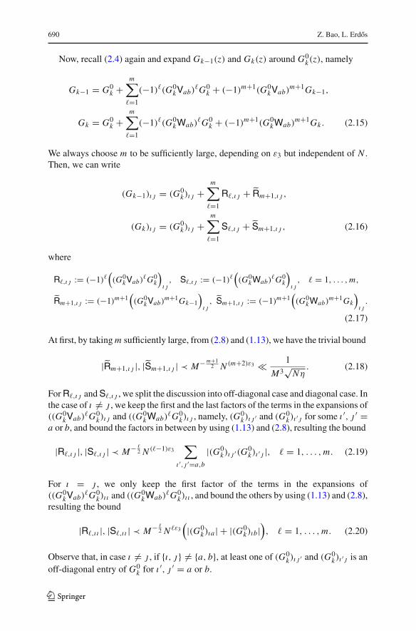
690 Z. Bao, L. Erdos
Now, recall (2.4) again and expand Gk−1(z) and Gk(z) around G0k(z), namely
Gk−1 = G0k +
m∑
�=1
(−1)�(G0kVab)
�G0k + (−1)m+1(G0
kVab)m+1Gk−1,
Gk = G0k +
m∑
�=1
(−1)�(G0kWab)
�G0k + (−1)m+1(G0
kWab)m+1Gk . (2.15)
We always choose m to be sufficiently large, depending on ε3 but independent of N .Then, we can write
(Gk−1)ıj = (G0k)ıj +
m∑
�=1
R�,ıj +˜Rm+1,ıj ,
(Gk)ıj = (G0k)ıj +
m∑
�=1
S�,ıj +˜Sm+1,ıj , (2.16)
where
R�,ıj := (−1)�(
(G0kVab)
�G0k
)
ıj, S�,ıj := (−1)�
(
(G0kWab)
�G0k
)
ıj, � = 1, . . . ,m,
˜Rm+1,ıj := (−1)m+1(
(G0kVab)
m+1Gk−1
)
ıj, ˜Sm+1,ıj := (−1)m+1
(
(G0kWab)
m+1Gk
)
ıj.
(2.17)
At first, by takingm sufficiently large, from (2.8) and (1.13), we have the trivial bound
|˜Rm+1,ıj |, |˜Sm+1,ıj | ≺ M−m+12 N (m+2)ε3 1
M3√Nη. (2.18)
ForR�,ıj andS�,ıj , we split the discussion into off-diagonal case and diagonal case. Inthe case of ı �= j , we keep the first and the last factors of the terms in the expansions of((G0
kVab)�G0
k)ıj and ((G0kWab)
�G0k)ıj , namely, (G0
k)ıj ′ and (G0k)ı ′j for some ı ′, j ′ =
a or b, and bound the factors in between by using (1.13) and (2.8), resulting the bound
|R�,ıj |, |S�,ıj | ≺ M− �2 N (�−1)ε3
∑
ı ′,j ′=a,b
|(G0k)ıj ′(G
0k)ı ′j |, � = 1, . . . ,m. (2.19)
For ı = j , we only keep the first factor of the terms in the expansions of((G0
kVab)�G0
k)ı ı and ((G0kWab)
�G0k)ı ı , and bound the others by using (1.13) and (2.8),
resulting the bound
|R�,ı ı |, |S�,ı ı | ≺ M− �2 N �ε3
(
|(G0k)ıa | + |(G0
k)ıb|)
, � = 1, . . . ,m. (2.20)
Observe that, in case ı �= j , if {ı, j} �= {a, b}, at least one of (G0k)ıj ′ and (G
0k)ı ′j is an
off-diagonal entry of G0k for ı
′, j ′ = a or b.
123

Delocalization for a class of random block band matrices 691
Now we compare the 2nth moment of |(Gk−1)ıj | and |(Gk)ıj |. At first, we write
E|(Gd)ıj |2n = E((Gd)ıj )n((Gd)ıj )
n, d = k − 1, k. (2.21)
By substituting the expansion (2.16) into (2.21), we can write
E|(Gd)ıj |2n = A(ı, j)+ Rd(ı, j), d = k − 1, k, (2.22)
where A(ı, j) is the sum of the terms which depend only on H0k and the first four
moments of hab, and Rd(ı, j) is the sum of all the other terms. We claim that Rd(ı, j)satisfies the bound
|Rd(ı, j)| ≤ C Θ0
(
N ε3√M
)5(
δıj + δ{ı,j}{a,b}(Nη)n− 5
2
+ 1
(Nη)n
)
, d = k − 1, k,
(2.23)
for some positive constant C independent of n. Now, we verify (2.23). Accord-ing to (2.11) and the fact that the sequence R1,ıj , . . . ,Rm,ıj ,˜Rm+1,ıj , as well asS1,ıj , . . . ,Sm,ıj ,˜Sm+1,ıj , decreases by a factor N ε3/
√M in magnitude, it is not dif-
ficult to check the leading order terms of Rk−1(ı, j) are of the form
E
(
(G0k)ıj
)p (
(G0k)ıj
)2n−p−∑5�=1(q�+q ′
�)5∏
�=1
Rq��,ıj R
q ′�
�,ıj , (2.24)
with some p, q�, q ′� ∈ N such that
5∑
�=1
�(q� + q ′�) = 5, 0 ≤ p ≤ 2n −
5∑
�=1
(q� + q ′�), (2.25)
and the leading order terms of Rk(ı, j) possess the same form (withR replaced by S).Every other term has at least 6 factors of hab or h
gab or their conjugates, thus their sizes
are typically controlled by M−3(Nη)−n , i.e. they are subleading. Hence, it suffices tobound (2.24).
Now, the five factors of hab or hba within the R�,ıj ’s in (2.24) are independent ofthe rest and estimated by M−5/2. For the remaining factors from G0
k , we use (2.11)to bound 2n of them and use (2.8) to bound the rest. In the case that ı �= j and{ı, j} �= {a, b}, by the discussion above, we must have an off-diagonal entry of G0
kin the product (G0
k)ıj ′(G0k)ı ′j for any choice of ı ′, j ′ = a or b. Then, in the bound
for R�,ıj in (2.19), for each (G0k)ıj ′(G
0k)ı ′j , we keep the off-diagonal entry and bound
the other by N ε3 from assumption (2.8). Hence, by using (2.19) and (2.25), we seethat for some ır , jr ∈ {ı, j, a, b} with ır �= jr , r = 1, . . . ,
∑
(q� + q ′�), the following
123

692 Z. Bao, L. Erdos
bound holds
(2.24) ≤(
N ε3√M
)5
E
⎛
⎜
⎝|(G0
k)ıj |2n−∑5�=1(q�+q ′
�)
∑5�=1(q�+q ′
�)∏
r=1
|(G0k)ır jr |
⎞
⎟
⎠
≤ 3
(
N ε3√M
)5Θ0
(Nη)n, (2.26)
where the last step follows from (2.11) and Hölder’s inequality. In case of ı �= j but{ı, j} = {a, b}, we keep an entry in the product (G0
k)ıj ′(G0k)ı ′j and bound the other
by N ε3 . We remark here in this case the entry being kept can be either diagonal oroff-diagonal. Consequently, for some ır , jr ∈ {ı, j, a, b}, r = 1, . . . ,
∑
(q�+ q ′�), we
have the bound
(2.24) ≤(
N ε3√M
)5
E
⎛
⎜
⎝|(G0
k)ıj |2n−∑5�=1(q�+q ′
�)
∑5�=1(q�+q ′
�)∏
r=1
|(G0k)ır jr |
⎞
⎟
⎠
≤ 3
(
N ε3√M
)5Θ0
(Nη)n− 52
, (2.27)
by using (2.11) and Hölder’s inequality again. Hence, we have shown (2.23) in thecase of ı �= j . For ı = j , it is analogous to show
(2.24) ≤ 3
(
N ε3√M
)5Θ0 (2.28)
by using (2.11), (2.20) and Hölder’s inequality. Hence, we verified (2.23). Conse-quently, by Assumption 1.5, (2.22) and (2.23) we have
∣
∣
∣E|(Gk−1)ıj |2n − E|(Gk)ıj |2n∣
∣
∣ ≤ C Θ0
(
N ε3√M
)5(
δıj + δ{ı,j}{a,b}(Nη)n− 5
2
+ 1
(Nη)n
)
,
which together with the assumption (2.9) for E|(Gk−1)ıj |2n and the definition ofΘ�,ıj ’s in (2.6), we can get (2.10). Hence, we completed the proof of Lemma 2.3. ��
To show (2.1), we also need the following lemma.
Lemma 2.4 Suppose that the assumptions in Lemma 2.1 hold. Fix the indices a, b ∈{1, . . . N }. Let H0 be a matrix obtained from H with its (a, b)th entry replaced by 0.Then, if for some η0 ≥ 1/N there exists
|Gıı (z)| ≺ 1, |(G0)ı ı (z)| ≺ 1 for η ≥ η0, ∀ ı = 1, . . . , N , (2.29)
123

Delocalization for a class of random block band matrices 693
then we also have
|Gıj (z)| ≺ η0
η, |(G0)ıj (z)| ≺ η0
η, for
1
N< η ≤ η0, ∀ ı, j = 1, . . . , N .
Proof of Lemma 2.4 The proof is almost the same as the discussion on pages 2311–2312 in [10]. For the convenience of the reader, we sketch it below. At first, accordingto the discussion below (4.28) in [10], for any ı, j = 1, . . . , N , we have
|Gıj (E + iη)| ≤ C max�
∑
k≥0
ImG��(E + i2kη).
Now, we set k1 := max{k : 2kη < η0} and k2 := max{k : 2kη < 1}. According to ourassumption, both k1 and k2 are of the order log N . Now, we have
∑
k≥0
ImG��(E + i2kη) =k1∑
k=0
ImG��(E + i2kη)+k2∑
k=k1
ImG��(E + i2kη)
+∞∑
k=k2+1
ImG��(E + i2kη)
≺ η0
η
k1∑
k=0
1
2kImG��(E + iη0)+ (k2 − k1)+ 1 ≺ η0
η
where in the second step, we used the fact that the function y �→ yImG��(E + iy)is monotonically increasing, the condition (2.29) and the fact η ≤ η0. Hence, weconclude the proof of Lemma 2.4. ��
Now, with Theorem 1.15, Lemmas 2.3 and 2.4, we can prove Lemma 2.1.
Proof for Lemma 2.1 The proof relies on the following bootstrap argument, namely,we show that once
|(G�)ıj | ≺ 1, ∀ � = 1, . . . , ς(N ), ∀ ı, j = 1, . . . , N (2.30)
holds for η ≥ η0 with η0 ∈ [N−1+ε2+ε3 ,M−1N ε2 ], it also holds for η ≥ η0N−ε3 forany ε3 satisfying (2.5). Assuming (2.30) holds for η ≥ η0, we see that
maxı,j
|(G0�)ıj | = max
ı,j|(G�)ıj + ((G�)WabG
0�)ıj |
≺ maxı,j
|(G�)ıj |(
1 + 1√M
maxı,j
|(G0�)ıj |
)
≺ 1 + 1√M
maxı,j
|(G0�)ıj |.
123

694 Z. Bao, L. Erdos
Consequently, for η ≥ η0, we also have
|(G0�)ıj | ≺ 1, ∀ � = 1, . . . , ς(N ), ∀ ı, j = 1, . . . , N . (2.31)
Therefore, (2.29) holds. Then, by Lemma 2.4, we see that (2.8) holds for η ≥ η0N−ε3 .Furthermore, by Lemma 2.3 and Theorem 1.15 for G0, i.e. the Gaussian case, one canget that for any given n,
E|(G�)ıj |2n ≤ Θ�,ıj
(
δıj + 1
(Nη)n
)
≤ 2Θ0
(
δıj + 1
(Nη)n
)
,
for M−1N ε2 ≥ η ≥ η0N−ε3 ,∀ � = 1, . . . , ς(N ), ∀ ı, j = 1, . . . , N . (2.32)
Note that since (2.32) holds for any given n, we get (2.30) forM−1N ε2 ≥ η ≥ η0N−ε3 .Now we start from η0 = M−1N ε2 . By Proposition 1.7 we see that (2.30) holds for
all η ≥ η0. Then we can use the bootstrap argument above finitely many times to show(2.30) holds for all η ≥ N−1+ε2 . Consequently, we have (2.8) for all η ≥ N−1+ε2 .Then, Lemma 2.1 follows from Lemma 2.3 and Theorem 1.15 immediately. ��
2.2 Proof of Theorem 1.9
Without loss of generality we can assume that M ≤ N (log N )−10, otherwise, Propo-sition 1.7 implies (1.17) immediately. We only need to consider the diagonal entriesGii below, since the bound for the off-diagonal entires of G(z) is implied by (2.1)directly. For simplicity, we introduce the notation
Λd ≡ Λd(z) := maxi
|Gii (z)− msc(z)|.
To bound Λd , a key technical input is the estimate for the quantity
ζi ≡ ζi (z) := (Gii )−1 + z +
∑
a
σ 2aiGaa, (2.33)
which is given in the following lemma.
Lemma 2.5 Suppose that H satisfies Assumptions 1.1, 1.5 and 1.14. We have
maxi=1,...,N
|ζi (z)| ≺ (Nη)− 12 , (2.34)
for all z ∈ D(N , κ, ε2).
The proof of Lemma 2.5 will be postponed. Using Lemma 2.5, we see that, withhigh probability, (2.33) is a small perturbation of the self-consistent equation of msc,i.e. (1.14), considering
∑
a σ2ai = 1. To control Λd , we use a continuity argument
from [12].
123

Delocalization for a class of random block band matrices 695
We remind here that in the sequel, the parameter set of the stochastic dominance isalways D(N , κ, ε2), without further mention. We need to show that
Λd ≺ (Nη)− 12 , (2.35)
and first we claim that it suffices to show that
1(
Λd ≤ N− ε24
)
Λd ≺ (Nη)− 12 . (2.36)
Indeed, if (2.36) were proven, we see that with high probability either Λd > N− ε24
or Λd ≺ (Nη)− 12 ≤ N− ε2
2 for z ∈ D(N , κ, ε2). That means, there is a gap in thepossible range of Λd . Now, choosing ε in (1.15) to be sufficiently small, we are ableto get for η = M−1N ε2 ,
Λd ≺ N− ε22 , ∀ E ∈ [−2 + κ, 2 − κ], ∀ i = 1, . . . , N . (2.37)
By the fact that Λd is continuous in z, we see that with high probability, Λd canonly stay in one side of the range, namely, (2.35) holds. The rigorous details of thisargument involve considering a fine discrete grid of the z-parameter and using thatG(z) is Lipschitz continuous (albeit with a large Lipschitz constant 1/η). The detailsare found in Section 5.3 of [12].
Hence, what remains is to verify (2.36). The proof of (2.36) is almost the sameas that for Lemma 3.5 in [14]. For the convenience of the reader, we sketch it belowwithout reproducing the details. We set
m ≡ m(z) := 1
N
N∑
i=1
Gii (z), ui ≡ ui (z) := Gii − m, i = 1, . . . , N .
We also denote u := (u1, . . . ,uN ). By the assumption Λd ≤ N− ε24 , we have
ui = O(
N− ε24
)
. (2.38)
Now we rewrite (2.33) as
0 = Gii + 1
z +∑a σ2aiGaa − ζi
=: Gii + 1
z + m(z)+˜ζi . (2.39)
By using (2.34), Lemma 5.1 in [14], and the assumption Λd ≤ N− ε24 , we can show
that
˜ζi = −∑
a σ2aiua
(z + m(z))2+ O
(
||u||2∞)
+ O(
maxi
|ζi |)
. (2.40)
123
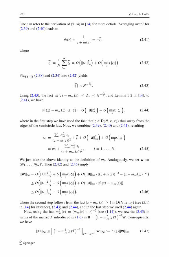
696 Z. Bao, L. Erdos
One can refer to the derivation of (5.14) in [14] for more details. Averaging over i for(2.39) and (2.40) leads to
m(z)+ 1
z + m(z)= −˜ζ , (2.41)
where
˜ζ := 1
N
N∑
i=1
˜ζi = O(
||u||2∞)
+ O(
maxi
|ζi |)
(2.42)
Plugging (2.38) and (2.34) into (2.42) yields
|˜ζ | ≺ N− ε22 . (2.43)
Using (2.43), the fact |m(z) − msc(z)| ≤ Λd ≤ N− ε24 , and Lemma 5.2 in [14], to
(2.41), we have
|m(z)− msc(z)| ≤ |˜ζ | = O(
||u||2∞)
+ O(
maxi
|ζi |)
, (2.44)
where in the first step we have used the fact that z ∈ D(N , κ, ε2) thus away from theedges of the semicircle law. Now, we combine (2.39), (2.40) and (2.41), resulting
ui =∑
a σ2aiua
(z + m(z))2+˜ζ + O
(
||u||2∞)
+ O(
maxi
|ζi |)
= wi +∑
a σ2aiua
(z + msc(z))2, i = 1, . . . , N . (2.45)
We just take the above identity as the definition of wi . Analogously, we set w :=(w1, . . . ,wN )
′. Then (2.42) and (2.45) imply
||w||∞ = O(
||u||2∞)
+ O(
maxi
|ζi |)
+ O(||u||∞ · |(z + m(z))−2 − (z + msc(z))
−2|)
≤ O(
||u||2∞)
+ O(
maxi
|ζi |)
+ O(||u||∞ · |m(z)− msc(z)|
)
≤ O(
||u||2∞)
+ O(
maxi
|ζi |)
, (2.46)
where the second step follows from the fact |z+msc(z)| ≥ 1 in D(N , κ, ε2) (see (5.1)in [14] for instance), (2.43) and (2.44), and in the last step we used (2.44) again.
Now, using the fact m2sc(z) = (msc(z) + z)−2 (see (1.14)), we rewrite (2.45) in
terms of the matrix T introduced in (1.6) as u = (1 − m2sc(z)T
)−1w. Consequently,we have
||u||∞ ≤∣
∣
∣
∣
∣
∣
(
1 − m2sc(z)T
)−1∣
∣
∣
∣
∣
∣
�∞→�∞||w||∞ := Γ (z)||w||∞. (2.47)
123

Delocalization for a class of random block band matrices 697
Then for z ∈ D(N , κ, ε2), using (1.7) and Proposition A.2 (ii) in [12] (with δ− = 1and θ > c), we can get
Γ (z) = O(log N ). (2.48)
Plugging (2.48) and (2.46) into (2.47) yields
||u||∞ ≺ O
(
||u||2∞ + O(
maxi
|ζi |)
)
≺ ||u||2∞ + (Nη)− 12 ,
where the second step follows from (2.34). Then (2.38) further implies that ||u||∞ ≺(Nη)− 1
2 , which together with (2.44) and (2.34) also implies
|m(z)− msc(z)| ≺ (Nη)− 12 .
Hence
Λd ≤ ||u||∞ + |m(z)− msc(z)| ≺ (Nη)− 12 .
Therefore, we completed the proof of Theorem 1.9.
Proof of Lemma 2.5 At first, recalling the notation defined in (1.3), we denote theGreen’s function of H (i) as
G(i)(z) := (H (i) − z)−1,
with a little abuse of notation. For simplicity, we omit the variable z from the notationbelow. At first, we recall the elementary identity by Schur’s complement, namely,
Gii =(
hii − z − (h〈i〉i )
∗G(i)h〈i〉i
)−1. (2.49)
where we used the notation h〈i〉i to denote the i th column of H , with the i th component
deleted. Now, we use the identity for a, b �= i (see Lemma 4.5 in [12] for instance),
G(i)ab = Gab − GaiGib(Gii )−1 = Gab − GaiGib
(
hii − z − (h〈i〉i )
∗G(i)h〈i〉i
)
.
(2.50)
By using (1.11) and the large deviation estimate for the quadratic form (see TheoremC.1 of [12] for instance), we have
∣
∣
∣
∣
∣
∣
(h〈i〉i )
∗G(i)h〈i〉i −
∑
a �=i
σ 2ai · G(i)aa
∣
∣
∣
∣
∣
∣
≺√
1
Mmaxa
|G(i)aa |2 + maxa �=b
|G(i)ab |2, (2.51)
123

698 Z. Bao, L. Erdos
which implies that
∣
∣
∣(h〈i〉i )
∗G(i)h〈i〉i
∣
∣
∣ ≺ maxa �=i
|G(i)aa | +√
1
Mmaxa �=i
|G(i)aa |2 + maxa �=b
|G(i)ab |2 ≤ 3 maxa,b �=i
|G(i)ab |,(2.52)
where we have used the fact that∑
a σ2ai = 1 in the first inequality above. Plugging
(1.22) and (2.52) into (2.50) and using Corollary 2.2 we obtain
maxa,b �=i
|G(i)ab | ≺ 1 + 1
Nη
(
1 + 3 maxa,b �=i
|G(i)ab |)
,
which implies
maxa,b �=i
|G(i)ab | ≺ 1,∣
∣
∣(h〈i〉i )
∗G(i)h〈i〉i
∣
∣
∣ ≺ 1. (2.53)
In addition, (1.22), (2.50) and (2.53) lead to the fact that
∣
∣
∣Gab(z)− G(i)ab(z)∣
∣
∣ ≺ 1
Nη,
∣
∣
∣G(i)ab(z)
∣
∣
∣ ≺ δab + (Nη)− 12 , ∀ a, b �= i. (2.54)
Now, using (2.33), (2.49), (2.51) and (2.54), we can see that
|ζi | =∣
∣
∣
∣
∣
−hii + (h〈i〉i )
∗G(i)h〈i〉i −
∑
a
σ 2aiGaa
∣
∣
∣
∣
∣
≺ (Nη)− 12 . (2.55)
Therefore, we completed the proof of Lemma 2.5. ��
2.3 Proof of Theorem 1.12
With Theorem 1.9, we can prove Theorem 1.12 routinely. At first, according to theuniform bound (1.18), we have
maxa,b
supz∈D(N ,κ,ε2)
|Gab(z)− δabmsc(z)| ≺ 1,
which implies that
maxa
supz∈D(N ,κ,ε2)
|Gaa(z)| ≺ 1 (2.56)
123

Delocalization for a class of random block band matrices 699
due to the fact that msc(z) ∼ 1. Recalling the normalized eigenvector ui = (ui1, . . . ,uiN ) corresponding to λi , and using the spectral decomposition, we have
maxa
ImGaa(z) = maxa
N∑
i=1
|uia |2η|λi − E |2 + η2 =
N∑
i=1
||ui ||2∞η|λi − E |2 + η2 . (2.57)
For any |λi | ≤ √2 − κ , we set E = λi on the r.h.s. of (2.57) and use (2.56) to bound
the l.h.s. of it. Then we obtain ||ui ||2∞/η ≺ 1. Choosing η = N−1+ε2 above and usingthe fact that ε2 can be arbitrarily small, we can get (1.19). Hence, we completed theproof of Theorem 1.12.
3 Supersymmetric formalism and integral representation for theGreen’s function
In this section, we will represent E|Gi j (z)|2n for the Gaussian case by a superintegral.The final representation is stated in (3.31). We make the convention here, for any realargument in an integral below, its region of the integral is always R, unless specifiedotherwise.
3.1 Gaussian integrals and superbosonization formulas
Let φ = (φ1, . . . , φk)′ be a vector of complex components, ψ = (ψ1, . . . , ψk)
′be a vector of Grassmann components. In addition, let φ∗ and ψ∗ be the conjugatetransposes of φ and ψ , respectively. We recall the following well-known formulas forGaussian integrals.
Proposition 3.1 (Gaussian integrals or Wick’s formulas)
(i) LetA be a k×k complex matrix with positive-definite Hermitian part, i.e.ReA >0. Then for any � ∈ N, and i1, . . . , i�, j1, . . . , j� ∈ {1, . . . , k}, we have∫ k∏
a=1
dReφadImφaπ
exp{−φ∗Aφ}�∏
b=1
φibφ jb = 1
det A
∑
σ∈P(�)
�∏
b=1
(A−1) jb,iσ(b) ,
(3.1)
where P(�) is the permutation group of degree �.(ii) Let B be any k × k matrix. Then for any � ∈ {0, . . . , k}, any � distinct integers
i1, . . . , i� and another � distinct integers j1, . . . , j� ∈ {1, . . . , k}, we have∫ k∏
a=1
dψadψa exp{−ψ∗Bψ}�∏
b=1
ψibψ jb = (−1)�+∑�α=1(iα+ jα) det B(I|J),
(3.2)
where I = {i1, . . . , i�}, and J = { j1, . . . , j�}.
123
700 Z. Bao, L. Erdos
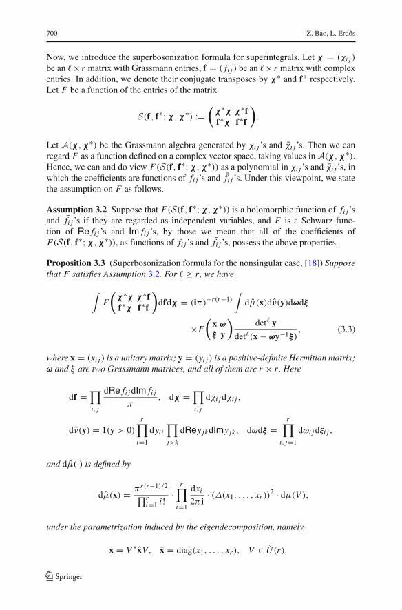
Now, we introduce the superbosonization formula for superintegrals. Let χ = (χi j )
be an �× r matrix with Grassmann entries, f = ( fi j ) be an �× r matrix with complexentries. In addition, we denote their conjugate transposes by χ∗ and f∗ respectively.Let F be a function of the entries of the matrix
S(f, f∗;χ ,χ∗) :=(
χ∗χ χ∗ff∗χ f∗f
)
.
Let A(χ ,χ∗) be the Grassmann algebra generated by χi j ’s and χi j ’s. Then we canregard F as a function defined on a complex vector space, taking values inA(χ ,χ∗).Hence, we can and do view F(S(f, f∗;χ ,χ∗)) as a polynomial in χi j ’s and χi j ’s, inwhich the coefficients are functions of fi j ’s and fi j ’s. Under this viewpoint, we statethe assumption on F as follows.
Assumption 3.2 Suppose that F(S(f, f∗;χ ,χ∗)) is a holomorphic function of fi j ’sand fi j ’s if they are regarded as independent variables, and F is a Schwarz func-tion of Re fi j ’s and Im fi j ’s, by those we mean that all of the coefficients ofF(S(f, f∗;χ ,χ∗)), as functions of fi j ’s and fi j ’s, possess the above properties.
Proposition 3.3 (Superbosonization formula for the nonsingular case, [18]) Supposethat F satisfies Assumption 3.2. For � ≥ r , we have
∫
F
(
χ∗χ χ∗ff∗χ f∗f
)
dfdχ = (iπ)−r(r−1)∫
dμ(x)dν(y)dωdξ
×F
(
x ω
ξ y
)
det� y
det�(x − ωy−1ξ), (3.3)
where x = (xi j ) is a unitary matrix; y = (yi j ) is a positive-definite Hermitian matrix;ω and ξ are two Grassmann matrices, and all of them are r × r . Here
df =∏
i, j
dRe fi jdIm fi jπ
, dχ =∏
i, j
dχi jdχi j ,
dν(y) = 1(y > 0)r∏
i=1
dyii∏
j>k
dRey jkdImy jk, dωdξ =r∏
i, j=1
dωi jdξi j ,
and dμ(·) is defined by
dμ(x) = πr(r−1)/2∏r
i=1 i !·
r∏
i=1
dxi2π i
· (Δ(x1, . . . , xr ))2 · dμ(V ),
under the parametrization induced by the eigendecomposition, namely,
x = V ∗xV, x = diag(x1, . . . , xr ), V ∈ U (r).
123

Delocalization for a class of random block band matrices 701
Here dμ(V ) is the Haar measure on U (r), andΔ(·) is the Vandermonde determinant.In addition, the integral w.r.t. x ranges over U (r), that w.r.t. y ranges over the cone ofpositive-definite matrices.
For the singular case, i.e. r > �, we only state the formula for the case of r = 2and � = 1, which is enough for our purpose. We can refer to formula (11) in [3] forthe result under more general setting.
Proposition 3.4 (Superbosonization formula for the singular case, [3]) Suppose thatF satisfies Assumption 3.2. If r = 2 and � = 1, we have
∫
F
(
χ∗χ χ∗ff∗χ f∗f
)
dfdχ = −1
π2
∫
dwdμ(x) · 1(y ≥ 0)dy
· dωdξF(
x ωw∗wξ yww∗
)
y(y − ξx−1ω)2
det2 x, (3.4)
where y is a positive variable; x is a 2-dimensional unitary matrix; ω = (ω1, ω2)′
and ξ = (ξ1, ξ2) are two vectors with Grassmann components. In addition, w is a unitvector, which can be parameterized by
w =(
v,√
1 − v2eiθ)′, v ∈ I, θ ∈ L.
Moreover, the differentials are defined as
dw = vdvdθ, dωdξ =∏
i=1,2
dωidξi .
In addition, the integral w.r.t. x ranges over U (2).
3.2 Initial representation
For a = 1, 2 and j = 1, . . . ,W , we set
Φa, j = (φa, j,1, . . . , φa, j,M)′, Ψa, j = (ψa, j,1, . . . , ψa, j,M
)′
Φa = (Φ ′a,1, . . . , Φ
′a,W
)′, Ψa = (Ψ ′
a,1, . . . , Ψ′a,W
)′.
For each j and each a, Φa, j is a vector with complex components, and Ψa, j is avector with Grassmann components. In addition, we use Φ∗
a, j and Ψ∗a, j to represent
the conjugate transposes of Φa, j and Ψa, j respectively. Analogously, we adopt thenotation Φ∗
a and Ψ ∗a to represent the conjugate transposes of Φa and Ψa , respec-
tively. We have the following integral representation for the moments of the Green’sfunction.
123

702 Z. Bao, L. Erdos
Lemma 3.5 For any p, q = 1, . . . ,W and α, β = 1, . . . ,M, we have
|Gpq,αβ(z)|2n = 1
(n!)2∫
dΦdΨ(
φ1,q,βφ1,p,αφ2,p,αφ2,q,β)n
× exp{
iΨ ∗1 (z − H)Ψ1 + iΦ∗
1 (z − H)Φ1
− iΨ ∗2 (z − H)Ψ2 − iΦ∗
2 (z − H)Φ2
}
, (3.5)
where
dΦ =∏
a=1,2
W∏
j=1
M∏
α′=1
dReφa, j,α′dImφa, j,α′
π, dΨ =
∏
a=1,2
W∏
j=1
M∏
α′=1
dψa, j,α′dψa, j,α′ .
Proof By using Proposition 3.1 (i) with � = n and Proposition 3.1 (ii) with � = 0, wecan get (3.5). ��
3.3 Averaging over the Gaussian random matrix
Recall the variance profile˜S in (1.2). Now,we take expectation of theGreen’s function,i.e average over the random matrix. By elementary Gaussian integral, we get
E|Gpq,αβ(z)|2n = 1
(n!)2∫
dΦdΨ(
φ1,q,βφ1,p,αφ2,p,αφ2,q,β)n
× exp
⎧
⎨
⎩
iW∑
j=1
(Tr X j J Z + TrY j J Z)
⎫
⎬
⎭
× exp
⎧
⎨
⎩
1
2M
∑
j,k
s jkT r X j J Xk J − 1
2M
∑
j,k
s jkT r Y j J Yk J
⎫
⎬
⎭
× exp
⎧
⎨
⎩
− 1
M
∑
j,k
s jkT rΩ j J Ξk J
⎫
⎬
⎭
, (3.6)
where J := diag(1,−1) and Z := diag(z, z), and for each j = 1, . . . ,W , thematricesX j , Y j , Ω j and Ξ j are 2 × 2 blocks of a supermatrix, namely,
S j =(
X j Ω j
Ξ j Y j
)
:=
⎛
⎜
⎜
⎜
⎝
Ψ ∗1, jΨ1, j Ψ
∗1, jΨ2, j Ψ
∗1, jΦ1, j Ψ
∗1, jΦ2, j
Ψ ∗2, jΨ1, j Ψ
∗2, jΨ2, j Ψ
∗2, jΦ1, j Ψ
∗2, jΦ2, j
Φ∗1, jΨ1, j Φ
∗1, jΨ2, j Φ
∗1, jΦ1, j Φ
∗1, jΦ2, j
Φ∗2, jΨ1, j Φ
∗2, jΨ2, j Φ
∗2, jΦ1, j Φ
∗2, jΦ2, j
⎞
⎟
⎟
⎟
⎠
.
Remark 3.6 The derivation of (3.6) from (3.5) is quite standard. We refer to the proofof (2.14) in [20] for more details and will not reproduce it here.
123

Delocalization for a class of random block band matrices 703
3.4 Decomposition of the supermatrices
From now on, we split the discussion into the following three cases
– (Case 1): Entries in the off-diagonal blocks, i.e. p �= q,– (Case 2): Off-diagonal entries in the diagonal blocks, i.e. p = q, α �= β,– (Case 3): Diagonal entries, i.e. p = q, α = β.
For each case, we will perform a decomposition for the supermatrix S j ( j = p or q).For a vector v and some index set I, we use v〈I〉 to denote the subvector obtained bydeleting the i th component of v for all i ∈ I. Then, we adopt the notation
S〈I〉j =
(
X 〈I〉j Ω
〈I〉j
Ξ〈I〉j Y 〈I〉
j
)
, S[i]j =
(
X [i]j Ω
[i]j
Ξ[i]j Y [i]
j
)
.
Here, for A = X j , Y j , Ω j or Ξ j , the notation A〈I〉 is defined via replacingΦa, j , Ψa, j ,
Φ∗a, j and Ψ
∗a, j by Φ
〈I〉a, j , Ψ
〈I〉a, j , (Φ
∗a, j )
〈I〉 and (Ψ ∗a, j )
〈I〉, respectively, for a = 1, 2, in the
definition of A. In addition, the notation A[i] is defined via replacing Φa, j , Ψa, j , Φ∗a, j
and Ψ ∗a, j by φa, j,i , ψa, j,i , φa, j,i and ψa, j,i respectively, for a = 1, 2, in the definition
of A. Moreover, for A = S j , X j , Y j , Ω j or Ξ j , we will simply abbreviate A〈{a,b}〉 andA〈{a}〉 by A〈a,b〉 and A〈a〉, respectively. Note that S[i]
j is of rank-one.Recalling the spatial-orbital parametrization for the rows or columns of H , it is
easy to see from the block structure that for any α, α′ ∈ {1, . . . ,M}, exchanging the( j, α)th row with the ( j, α′)th row and simultaneously exchanging the correspondingcolumns will not change the distribution of H .
For Case 1, due to the symmetry mentioned above, we can assume α = β = 1.Then we extract two rank-one supermatrices from Sp and Sq such that the quanti-ties φ2,p,1φ1,p,1 and φ1,q,1φ2,q,1 can be expressed in terms of the entries of thesesupermatrices. More specifically, we decompose the supermatrices
Sp = S〈1〉p + S[1]
p , Sq = S〈1〉q + S[1]
q . (3.7)
Consequently, we can write
φ1,q,1φ1,p,1φ2,p,1φ2,q,1 =(
Y [1]q
)
12
(
Y [1]p
)
21. (3.8)
For Case 2, due to symmetry, we can assume that α = 1, β = 2. Then we extracttwo rank-one supermatrices from Sp, namely,
Sp = S〈1,2〉p + S[1]
p + S[2]p . (3.9)
Consequently, we can write
φ1,p,2φ1,p,1φ2,p,1φ2,p,2 = (Y [2]p )12(Y
[1]p )21. (3.10)
123

704 Z. Bao, L. Erdos
Finally, for Case 3, due to symmetry, we can assume that α = 1. Then we extractonly one rank-one supermatrix from Sp, namely,
Sp = S〈1〉p + S[1]
p . (3.11)
Consequently, we can write
φ1,p,1φ1,p,1φ2,p,1φ2,p,1 =(
Y [1]p
)
12
(
Y [1]p
)
21=(
Y [1]p
)
11
(
Y [1]p
)
22.
Since the discussion for all three cases are similar, we will only present the detailsfor Case 1. More specifically, in the remaining part of this section and Sect. 4 toSect. 10, we will only treat Case 1. In Sect. 11, we will sum up the discussions in theprevious sections and explain how to adapt them to Case 2 and Case 3, resulting afinal proof of Theorem 1.15.
3.5 Variable reduction by superbosonization formulae
Wewill work with Case 1. Recall the decomposition (3.7). We use the superbosoniza-tion formulae to reduce the number of variables. We shall treat Sk(k �= p, q) andS〈1〉j ( j = p, q) on an equal footing and use the formula (3.3) with r = 2, � = M
for the former and r = 2, � = M − 1 for the latter, while we separate the termsS[1]j ( j = p, q) and use the formula (3.4). For simplicity, we introduce the notation
˜S j ={ S j , if j �= p, q,
S〈1〉j , if j = p, q.
(3.12)
Accordingly, we will use ˜X j , ˜Ω j , ˜Ξ j and ˜Y j to denote four blocks of ˜S j . With thisnotation, we can rewrite (3.6) with α = β = 1 as
E|Gpq,11(z)|2n = 1
(n!)2∫
dΦdΨ(
φ1,q,1φ1,p,1φ2,p,1φ2,q,1)n
× exp
⎧
⎨
⎩
iW∑
j=1
(
Tr˜X j J Z + Tr˜Y j J Z)
⎫
⎬
⎭
× exp
⎧
⎨
⎩
1
2M
∑
j,k
s jk
(
Tr˜X j J˜Xk J − Tr˜Y j J˜Yk J)
⎫
⎬
⎭
× exp
⎧
⎨
⎩
− 1
M
∑
j,k
s jkT r ˜Ω j J ˜Ξk J
⎫
⎬
⎭
×∏
k=p,q
exp{
iTr X [1]k J Z + iTrY [1]
k J Z}
123
Delocalization for a class of random block band matrices 705
×∏
k=p,q
exp
⎧
⎨
⎩
1
M
W∑
j=1
s jk
(
Tr˜X j J X[1]k J − Tr˜Y j J Y
[1]k J
)
⎫
⎬
⎭
×∏
k,�=p,q
exp
{
sk�
2M
(
Tr X [1]k J X [1]
� J − TrY [1]k J Y [1]
� J)
}
×∏
k,�=p,q
exp
{
− sk�
MTrΩ [1]
k J Ξ [1]� J
}
×∏
k=p,q
exp
⎧
⎨
⎩
− 1
M
∑
j
s jk
(
Tr ˜Ω j J Ξ[1]k J + TrΩ [1]
k J ˜Ξ j J)
⎫
⎬
⎭
, (3.13)
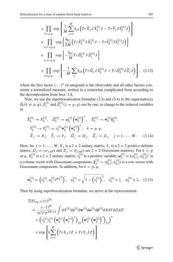
where the first factor (· · · )n of integrand is the observable and all other factors con-stitute a normalized measure, written in a somewhat complicated form according tothe decomposition from Sect. 3.4.
Now, we use the superbosonization formulae (3.3) and (3.4) to the supermatricesSk(k �= p, q), S〈1〉
j and S[1]j ( j = p, q) one by one, to change to the reduced variables
as
X [1]k → X [1]
k , Ω[1]k → ω
[1]k
(
w[1]k
)∗, Ξ
[1]k → w[1]
k ξ[1]k ,
Y [1]k → Y [1]
k := y[1]k w[1]
k
(
w[1]k
)∗, k = p, q,
˜X j → X j , ˜Y j → Y j , ˜Ω j → Ω j , ˜Ξ j → Ξ j , j = 1, . . . ,W. (3.14)
Here, for j = 1, . . . ,W, X j is a 2 × 2 unitary matrix; Y j is a 2 × 2 positive-definitematrix; Ω j = (ω j,αβ) and Ξ j = (ξ j,αβ) are 2 × 2 Grassmann matrices. For k = p
or q, X [1]k is a 2 × 2 unitary matrix; y[1]
k is a positive variable; ω[1]k = (ω[1]
k,1, ω[1]k,2)
′ isa column vector with Grassmann components; ξ [1]
k = (ξ [1]k,1, ξ[1]k,2) is a row vector with
Grassmann components. In addition, for k = p, q,
w[1]k =
(
v[1]k , u
[1]k eiσ [1]
k
)′, u[1]
k =√
1 −(
v[1]k
)2, v
[1]k ∈ I, σ
[1]k ∈ L. (3.15)
Then by using superbosonization formulae, we arrive at the representation
E|Gpq,11(z)|2n
= (−1)W
(n!)2π2W+4
∫
dX [1]dy[1]dw[1]dω[1]dξ [1]dXdYdΩdΞ
×(
y[1]p y[1]
q
(
w[1]q
(
w[1]q
)∗)
12
(
w[1]p
(
w[1]p
)∗)
21
)n
× exp
⎧
⎨
⎩
iW∑
j=1
(
Tr X j J Z + TrY j J Z)
⎫
⎬
⎭
123

706 Z. Bao, L. Erdos
× exp
⎧
⎨
⎩
1
2M
∑
j,k
s jk
(
Tr X j J Xk J − TrY j JYk J)
⎫
⎬
⎭
× exp
⎧
⎨
⎩
− 1
M
∑
j,k
s jkT rΩ j JΞk J
⎫
⎬
⎭
∏
j
detM Y j
detM(
X j −Ω j Y−1j Ξ j
)
×∏
k=p,q
det(
Xk −ΩkY−1k Ξk
)
det Yk
∏
k=p,q
exp{
iTr X [1]k J Z + iTrY [1]
k J Z}
×∏
k=p,q
exp
⎧
⎨
⎩
1
M
W∑
j=1
s jk
(
Tr X j J X[1]k J − TrY j JY
[1]k J
)
⎫
⎬
⎭
×∏
k,�=p,q
exp
{
sk�
2M
(
Tr X [1]k J X [1]
� J − TrY [1]k JY [1]
� J)
}
×∏
k,�=p,q
exp
{
− sk�
MTrω[1]
k (w[1]k )
∗ Jw[1]� ξ
[1]� J
}
×∏
k=p,q
exp
⎧
⎨
⎩
− 1
M
W∑
j=1
s jkT rΩ j Jw[1]k ξ
[1]k J
⎫
⎬
⎭
×∏
k=p,q
exp
⎧
⎨
⎩
− 1
M
W∑
j=1
s jkT rω[1]k (w
[1]k )
∗ JΞ j J
⎫
⎬
⎭
×∏
k=p,q
y[1]k
(
y[1]k − ξ
[1]k (X
[1]k )
−1ω[1]k
)2
det2(X [1]k )
, (3.16)
where we used the notation y[1] := (y[1]p , y
[1]q ),w[1] := (w[1]
p ,w[1]q ). The differentials
are defined by
dX [1] =∏
j=p,q
dμ(
X [1]j
)
, dy[1] =∏
j=p,q
1(
y[1]j > 0
)
dy[1]j ,
dw[1] =∏
j=p,q
dw[1]j =
∏
j=p,q
v[1]j dv[1]j dσ [1]
j , dω[1]dξ [1] =∏
α=1,2
∏
j=p,q
dω[1]j,αdξ
[1]j,α,
dX =W∏
j=1
dμ(X j ), dY =W∏
j=1
dν(Y j ), dΩdΞ =∏
α,β=1,2
W∏
j=1
dω j,αβdξ j,αβ .
Now we change the variables as X j J → X j ,Y j J → Bj ,Ω j J → Ω j , Ξ j J →Ξ j and perform the scaling X j → −MX j , Bj → MBj ,Ω j → √
MΩ j and Ξ j →
123

Delocalization for a class of random block band matrices 707
√MΞ j . Consequently, we can write
E|Gpq,11(z)|2n = (−1)WM4W
(n!)2π2W+4
∫
dX [1]dy[1]dw[1]dω[1]dξ [1]dXdBdΩdΞ
× exp{
− M(
K (X)+ L(B))
}
× P(Ω,Ξ, X, B) · Q(Ω,Ξ,ω[1], ξ [1], X [1], y[1],w[1])
× F(
X, B, X [1], y[1],w[1]), (3.17)
where the functions in the integrand are defined as
K (X) := −1
2
∑
j,k
s jkT r X j Xk + iE∑
j
T r X j +∑
j
log det X j ,
L(B) := 1
2
∑
j,k
s jkT r B j Bk − iE∑
j
T r B j −∑
j
log det Bj ,
P(Ω,Ξ, X, B)
:= exp
⎧
⎨
⎩
−∑
j,k
s jkT rΩ jΞk
⎫
⎬
⎭
×∏
j
1
detM(
1 + 1M X−1
j Ω j B−1j Ξ j
)
×∏
k=p,q
det(
Xk + 1MΩk B
−1k Ξk
)
det Bk, (3.18)
Q(Ω,Ξ,ω[1], ξ [1], X [1], y[1],w[1]) :=∏
k=p,q
(
1 − (y[1]k )
−1ξ[1]k (X
[1]k )
−1ω[1]k
)2
×∏
k=p,q
exp
⎧
⎨
⎩
− 1√M
∑
j
s jk
(
TrΩ jw[1]k ξ
[1]k J + Trω[1]
k (w[1]k )
∗ JΞ j
)
⎫
⎬
⎭
×∏
k,�=p,q
exp
{
− 1
Msk�Trω
[1]k (w
[1]k )
∗ Jw[1]� ξ
[1]� J
}
F(X, B, X [1], y[1],w[1]) := f (X, X [1]) g(B, y[1],w[1]), (3.19)
with
f (X, X [1]) := exp
⎧
⎨
⎩
MηW∑
j=1
Tr X j J
⎫
⎬
⎭
∏
k,�=p,q
exp
{
sk�
2MTr X [1]
k J X [1]� J
}
×∏
k=p,q
1
det2(
X [1]k
) exp
⎧
⎨
⎩
iTr X [1]k J Z −
∑
j
s jkT r X j X[1]k J
⎫
⎬
⎭
,
(3.20)
123
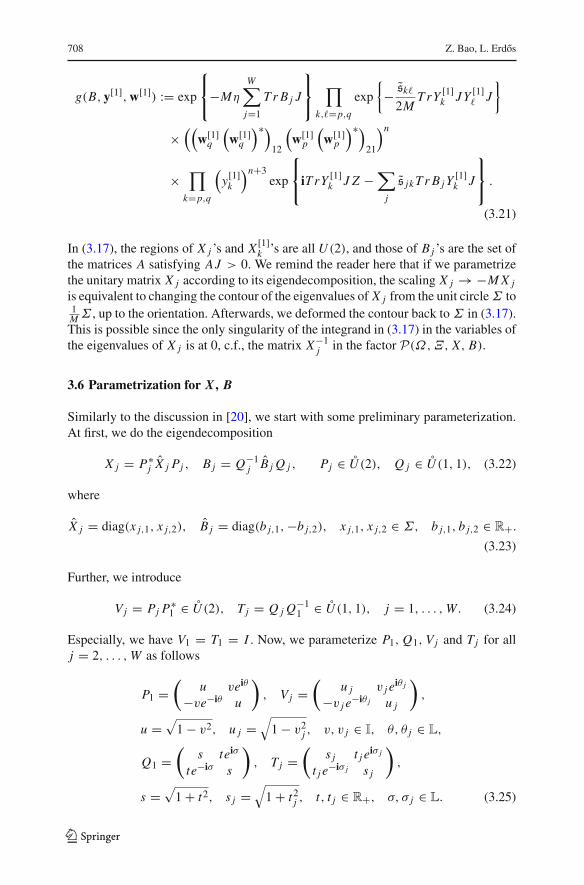
708 Z. Bao, L. Erdos
g(B, y[1],w[1]) := exp
⎧
⎨
⎩
−MηW∑
j=1
Tr B j J
⎫
⎬
⎭
∏
k,�=p,q
exp
{
− sk�
2MTrY [1]
k JY [1]� J
}
×((
w[1]q
(
w[1]q
)∗)
12
(
w[1]p
(
w[1]p
)∗)
21
)n
×∏
k=p,q
(
y[1]k
)n+3exp
⎧
⎨
⎩
iTrY [1]k J Z −
∑
j
s jkT r B jY[1]k J
⎫
⎬
⎭
.
(3.21)
In (3.17), the regions of X j ’s and X [1]k ’s are all U (2), and those of Bj ’s are the set of
the matrices A satisfying AJ > 0. We remind the reader here that if we parametrizethe unitary matrix X j according to its eigendecomposition, the scaling X j → −MX j
is equivalent to changing the contour of the eigenvalues of X j from the unit circleΣ to1MΣ , up to the orientation. Afterwards, we deformed the contour back toΣ in (3.17).This is possible since the only singularity of the integrand in (3.17) in the variables ofthe eigenvalues of X j is at 0, c.f., the matrix X−1
j in the factor P(Ω,Ξ, X, B).
3.6 Parametrization for X, B
Similarly to the discussion in [20], we start with some preliminary parameterization.At first, we do the eigendecomposition
X j = P∗j X j Pj , Bj = Q−1
j B j Q j , Pj ∈ U (2), Q j ∈ U (1, 1), (3.22)
where
X j = diag(x j,1, x j,2), B j = diag(b j,1,−b j,2), x j,1, x j,2 ∈ Σ, b j,1, b j,2 ∈ R+.(3.23)
Further, we introduce
Vj = Pj P∗1 ∈ U (2), Tj = Q j Q
−11 ∈ U (1, 1), j = 1, . . . ,W. (3.24)
Especially, we have V1 = T1 = I . Now, we parameterize P1, Q1, Vj and Tj for allj = 2, . . . ,W as follows
P1 =(
u veiθ
−ve−iθ u
)
, Vj =(
u j v j eiθ j
−v j e−iθ j u j
)
,
u =√
1 − v2, u j =√
1 − v2j , v, v j ∈ I, θ, θ j ∈ L,
Q1 =(
s teiσ
te−iσ s
)
, Tj =(
s j t j eiσ j
t j e−iσ j s j
)
,
s =√
1 + t2, s j =√
1 + t2j , t, t j ∈ R+, σ, σ j ∈ L. (3.25)
123

Delocalization for a class of random block band matrices 709
Under the parametrization above, we can express the corresponding differentials asfollows.
dXdB = dμ(P1)dν(Q1) ·W∏
j=2
dμ(Vj )dν(Tj ) ·W∏
j=1
db j,1db j,2 · dx j,12π i
dx j,22π i
×2W (π/2)2WW∏
j=1
(x j,1 − x j,2)2(b j,1 + b j,2)
2, (3.26)
where
dμ(P1) = 2vdv · dθ2π, dμ(Vj ) = 2v jdv j · dθ j
2π, dν(Q1) = 2tdt · dσ
2π,
dν(Tj ) = 2t jdt j · dσ j2π.
In addition, for simplicity, we do the change of variables
Ω j → P∗1Ω j Q1, Ξ j → Q−1
1 Ξ j P1. (3.27)
Note that the Berezinian of such a change is 1. After this change, P(Ω,Ξ, X, B, y[1],w[1]) turns out to be independent of P1 and Q1.
To adapt to the new parametrization, we change the notation
K (X)→ K (X , V ), L(B)→ L(B, T ), P(Ω,Ξ, X, B)→ P(Ω,Ξ, X , B, V, T ),Q(Ω,Ξ,ω[1], ξ [1], X [1], y[1],w[1])→ Q(Ω,Ξ,ω[1], ξ [1], P1, Q1, X
[1], y[1],w[1]),F(X, B, X [1], y[1],w[1])→ F(X , B, V, T, P1, Q1, X
[1], y[1],w[1]), (3.28)
f (X, X [1])→ f (P1, V, X , X[1]), g(B, y[1],w[1])→ g(Q1, T, B, y[1],w[1]).
We recall here that K (X) does not depend on P1, as well, L(B) does not depend onQ1. Moreover, according to the change (3.27), we have
P(Ω,Ξ, X , B, V, T ) = exp
⎧
⎨
⎩
−∑
j,k
s jkT rΩ jΞk
⎫
⎬
⎭
×∏
j
1
detM(
1 + M−1V ∗j X
−1j V jΩ j T
−1j B−1
j TjΞ j)
×∏
k=p,q
det(
V ∗k XkVk + M−1ΩkT
−1k B−1
k TkΞk)
det Bk(3.29)
and
Q(
Ω,Ξ,ω[1], ξ [1], P1, Q1, X[1], y[1],w[1])
123
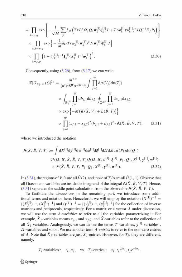
710 Z. Bao, L. Erdos
=∏
k=p,q
exp
⎧
⎨
⎩
− 1√M
∑
j
s jk(
Tr P∗1Ω j Q1w[1]
k ξ[1]k J + Trω[1]
k (w[1]k )
∗ J Q−11 Ξ j P1
)
⎫
⎬
⎭
×∏
k,�=p,q
exp{
− 1
Msk�Trω
[1]k (w
[1]k )
∗ J (w[1]� )ξ
[1]� J
}
×∏
k=p,q
(
1 − (y[1]k )
−1ξ[1]k (X
[1]k )
−1ω[1]k
)2. (3.30)
Consequently, using (3.26), from (3.17) we can write
E|Gpq,11(z)|2n = M4W
(n!)28Wπ2W+4
∫ W∏
j=2
dμ(Vj )dν(Tj )
×∫
R2W+
W∏
j=1
db j,1db j,2
∮
Σ2W
W∏
j=1
dx j,1dx j,2
× exp{
−M(
K (X , V )+ L(B, T ))
}
×W∏
j=1
(x j,1 − x j,2)2(b j,1 + b j,2)
2 · A(X , B, V, T ). (3.31)
where we introduced the notation
A(X , B, V, T ) :=∫
dX [1]dy[1]dw[1]dω[1]dξ [1]dΩdΞdμ(P1)dν(Q1)
P(Ω,Ξ, X , B, V, T )Q(Ω,Ξ,ω[1], ξ [1], P1, Q1, X[1], y[1],w[1])
× F(X , B, V, T, P1, Q1, X[1], y[1],w[1]). (3.32)
In (3.31), the regions of Vj ’s are all U (2), and those of Tj ’s are all U (1, 1). Observe thatall Grassmann variables are inside the integrand of the integralA(X , B, V, T ). Hence,(3.31) separates the saddle point calculation from the observable A(X , B, V, T ).
To facilitate the discussions in the remaining part, we introduce some addi-tional terms and notation here. Henceforth, we will employ the notation (X [1])−1 ={(X [1]
p )−1, (X [1]
q )−1} and (y[1])−1 = {(y[1]
p )−1, (y[1]
q )−1} for the collection of inverse
matrices and reciprocals, respectively. For a matrix or a vector A under discussion,we will use the term A-variables to refer to all the variables parametrizing it. Forexample, X j -variables means x j,1 and x j,2, and X -variables refer to the collection ofall X j -variables. Analogously, we can define the terms T -variables, y[1]-variables ,Ω-variables and so on. We use another term A-entries to refer to the non-zero entriesof A. Note that X j -variables are just X j -entries. However, for Tj , they are different,namely,
Tj -variables : t j , σ j , vs. Tj -entries : s j , t j eiσ j , t j e
−iσ j .
123
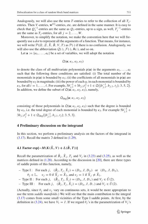
Delocalization for a class of random block band matrices 711
Analogously, we will also use the term T -entries to refer to the collection of all Tj -entries. Then V -entries, w[1]-entries, etc. are defined in the same manner. It is easy tocheck that Q−1
1 -entries are the same as Q1-entries, up to a sign, as well, T−1j -entries
are the same as Tj -entries, for all j = 2, . . . ,W .Moreover, to simplify the notation, we make the convention here that we will fre-
quently use a dot to represent all the arguments of a function. That means, for instance,we will write P(Ω,Ξ, X , B, V, T ) as P(·) if there is no confusion. Analogously, wewill also use the abbreviation Q(·),F(·),A(·), and so on.
Let a := {a1, . . . , a�} be a set of variables, we will adopt the notation
Q(a; κ1, κ2, κ3)
to denote the class of all multivariate polynomials p(a) in the arguments a1, . . . , a�such that the following three conditions are satisfied: (i) The total number of themonomials in p(a) is bounded by κ1; (ii) the coefficients of all monomials in p(a) arebounded by κ2 inmagnitude; (iii) the power of each ai in eachmonomial is bounded byκ3, for all i = 1, . . . , �. For example, 5b−1
j,1+3b j,1t2j +1 ∈ Q({b−1
j,1, b j,1, t j }; 3, 5, 2)
.In addition, we define the subset of Q(a; κ1, κ2, κ3), namely,
Qdeg(
a; κ1, κ2, κ3)
consisting of those polynomials in Q(a; κ1, κ2, κ3) such that the degree is boundedby κ3, i.e. the total degree of each monomial is bounded by κ3. For example 5b−1
j,1 +3b j,1t2j + 1 ∈ Qdeg
({b−1j,1, b j,1, t j }; 3, 5, 3
)
.
4 Preliminary discussion on the integrand
In this section, we perform a preliminary analysis on the factors of the integrand in(3.17). Recall the matrix I defined in (1.29).
4.1 Factor exp{−M(K (X, V ) + L(B, T ))}
Recall the parametrization of B j , X j , Tj and Vj in (3.23) and (3.25), as well as thematrices defined in (1.28). According to the discussion in [20], there are three typesof saddle points of this function, namely,
– Type I : For each j , (B j , Tj , X j ) = (D±, I, D±) or (D±, I, D∓),θ j ∈ L, v j = 0 if X j = X1, and v j = 1 if X j �= X1.
– Type II : For each j , (B j , Tj , X j ) = (D±, I, D+) and Vj ∈ U (2).– Type III : For each j , (B j , Tj , X j ) = (D±, I, D−) and Vj ∈ U (2).
(Actually, since θ j and v j vary on continuous sets, it would be more appropriate touse the term saddle manifolds.) We will see that the main contribution to the integral(3.17) comes from some small vicinities of the Type I saddle points. At first, by thedefinition in (3.24), we have V1 = I . If we regard θ j ’s in the parametrization of Vj ’s
123

712 Z. Bao, L. Erdos
as fixed parameters, it is easy to see that there are totally 2W choices of Type I saddlepoints. Furthermore, the contributions from all the Type I saddle points are the same,since one can always do the transform Vj → IVj or (X j , Pj ) → (IX jI,IPj ) forseveral j to change one saddle to another. That means, for Type I saddle points, itsuffices to consider
– Type I’ : For each j , (B j , Tj , X j , Vj ) = (D±, I, D±, I ).
Therefore, the total contribution to the integral (3.17) from all Type I saddle points is2W times that from the Type I’ saddle point.
Following the discussion in [20], we will show in Sect. 5 that both K (X , V ) −K (D±, I ) and L(B, T ) − L(D±, I ) have positive real parts, bounded by somepositive quadratic forms from below, which allows us to perform the saddle pointanalysis. In addition, it will be seen that in a vicinity of the Type I’ saddle point,exp{−M(K (X , V )+ L(B, T ))} is approximately Gaussian.
4.2 Factor Q(Ω,Ξ,ω[1], ξ [1], P1, Q1, X [1], y[1], w[1])
The functionQ(·) contains both theΩ,Ξ -variables from P(·), and the P1, Q1, X [1],y[1],w[1]-variables from F(·). In addition, note that in the integrand in (3.17), Q(·)is the only factor containing the ω[1] and ξ [1]- variables. Hence, we can compute theintegral
Q(
Ω,Ξ, P1, Q1, X[1], y[1],w[1])
:=∫
dω[1]dξ [1] Q(
Ω,Ξ,ω[1], ξ [1], P1, Q1, X[1], y[1],w[1]) (4.1)
At first, the explicit formula forQ(·) is complicated and irrelevant for us. From (3.30)and the definition of the Grassmann integral, it is not difficult to see thatQ(·) is a poly-nomial of the (X [1])−1, (y[1])−1,w[1], P1, Q1,Ω andΞ -entries. In principle, for eachmonomial in the polynomialQ(·), we can combine theGrassmann variables withP(·),then perform the integral overΩ andΞ -variables,whilstwe combine the complex vari-ables with F(·), and perform the integral over X [1], y[1],w[1], P1 and Q1-variables.A formal discussion on Q(·) will be given in Sect. 6.1. However, the terms from Q(·)turn out to be irrelevant in our proof. Therefore, in the arguments with Q(·) involved,a typical strategy that we will adopt is as follows: we usually neglectQ(·) at first, andperform the discussion on P(·) and F(·) separately, at the end, we make necessarycomments on how to slightly modify the discussions to take Q(·) into account.
4.3 Factor P(Ω,Ξ, X, B, V, T )
We will mainly regard P(·) as a function of the Ω and Ξ -variables. As mentionedabove, we also have some Ω and Ξ -variables from the irrelevant term Q(·). But wetemporarily ignore them and regard as if the integral over Ω and Ξ -variables reads
P(X , B, V, T ) :=∫
dΩdΞ P(Ω,Ξ, X , B, V, T ). (4.2)
123

Delocalization for a class of random block band matrices 713
We shall estimateP(·) in three different regions: (1) the complement of the vicinities ofthe saddle points; (2) the vicinity of Type I saddle point; (3) the vicinities of Type II andIII saddle points,whichwill be done inSects. 6.2, 9.1 and10.1, respectively. (Definition5.5 gives the precise definition of the vicinities.) In each case we will decompose thefunction P(·) as a product of a Gaussian measure and a multivariate polynomial ofGrassmann variables. Consequently, we can employ (3.2) to perform the integral ofthis polynomial against the Gaussian measure, whereby P(·) can be estimated.
4.4 Factor F(X, B, V, T, P1, Q1, X [1], y[1], w[1])
Observe that F is the only term containing the energy scale η. As in the previousdiscussion of P(·), here we also ignore the P1, Q1, X [1], y[1],w[1]-variables from theirrelevant term Q(·) temporarily, and investigate the integral
F(X , B, V, T ) =∫
dX [1]dy[1]dw[1]dμ(P1)dν(Q1)
× F(X , B, V, T, P1, Q1, X[1], y[1],w[1])
=∫
dX [1]dμ(P1) f (X , V, P1)
×∫
dy[1]dw[1]dν(Q1) g(B, T, Q1, y[1],w[1]). (4.3)
We shall also estimate F(·) in three different regions: (1) the complement of thevicinities of the saddle points; (2) the vicinity of Type I saddle point; (3) the vicinitiesof Type II and III saddle points, which will be done in Sects. 6.3, 9.2 and 10.2,respectively.
Especially, when we restrict the X , B, V and T -variables to the vicinity of the TypeI saddle points, the above integral can be performed approximately, resulting our mainterm, a factor of order 1/(Nη)n+2. This step will be done in Sect. 9. It is instructiveto give a heuristic sketch of this calculation. At first, we plug the Type I saddle pointsinto (4.3). We will show that the integral of f (·) approximately reads
e−(a+−a−)Nη∫
dX [1]dμ(P1) f (D±, I, P1) ∼ 1
Nη,
which is the easy part. Then, recalling the definition of g(·) in (3.21) and the parame-terization (3.15), we will show that the integral of g(·) approximately reads
e(a+−a−)Nη∫
dy[1]dw[1]dν(Q1) g(D±, I, Q1, y[1],w[1])
∼∫ ∞
02tdt
∫
L2dσ [1]
p dσ [1]q einσ [1]
p e−inσ [1]q · e−cNηt2+c1e
−iσ [1]p t+c2eiσ [1]q t
∼∫ ∞
02tdt · t2n · e−cNηt2 ∼ 1
(Nη)n+1 , (4.4)
123

714 Z. Bao, L. Erdos
where in the second step above we used the fact that
∫
L
dσ · einσ ece−iσ t ∼ tn .
We notice that the factor einσ [1]p e−inσ [1]
q in (4.4) actually comes from the term(
(
w[1]q (w
[1]q )
∗)12
(
w[1]p (w
[1]p )
∗)21
)nin (3.21). This factor brings a strong oscillation
to the integrand in the integral (4.4). In Case 2, an analogous factor will appear, result-ing the same estimate as (4.4). However, in Case 3, such an oscillating factor is absent,then the estimate for the counterpart of the integral in (4.4) is of order 1/Nη insteadof 1/(Nη)n+1. The detailed analysis will be presented in Sects. 10 and 11.
5 Saddle points and vicinities
In this section, we study the saddle points of K (X , V ) and L(B, T ) and deform thecontours of the B-variables to pass through the saddle points. Then we introduce andclassify some small vicinities of these saddle points. The derivation of the saddlepoints of K (X , V ) and L(B, T ) in Sects. 5.1 and 5.2 below is essentially the sameas the counterpart in [20], the only difference is that we are working under a moregeneral setting on S. Hence, in Sects. 5.1 and 5.2, we just sketch the discussion, listthe results, and make necessary modifications to adapt to our setting. In the sequel,we employ the notation
ba := (b1,a, . . . , bW,a), xa := (x1,a, . . . , xW,a), a = 1, 2,
t := (t2, . . . , tW ), v := (v2, . . . , vW ),σ := (σ2, . . . , σW ), θ := (θ2, . . . , θW ). (5.1)
As mentioned above, later we also need to deform the contours, and discuss theintegral over some vicinities of the saddle points, thus it is convenient to intro-duce a notation for the integral over specific domains. To this end, for a = 1, 2,we use Iba and Ixa to denote generic domains of ba and xa respectively. Analo-gously, we use It and Iv to represent generic domains of t and v, respectively. Thesedomains will be specified later. Now, for some collection of domains, we introduce thenotation
I(
Ib1, Ib2, I
x1 , I
x2 , I
t , Iv)
:= M4W
(n!)28Wπ2W+4
∫
L2W−2
W∏
j=2
dθ j2π
W∏
j=2
dσ j2π
×∫
Ib1
W∏
j=1
db j,1
∫
Ib2
W∏
j=1
db j,2
∫
Ix1
W∏
j=1
dx j,1
×∫
Ix2
W∏
j=1
dx j,2
∫
It
W∏
j=2
2t jdt j
∫
Iv
W∏
j=2
2v jdv j
123
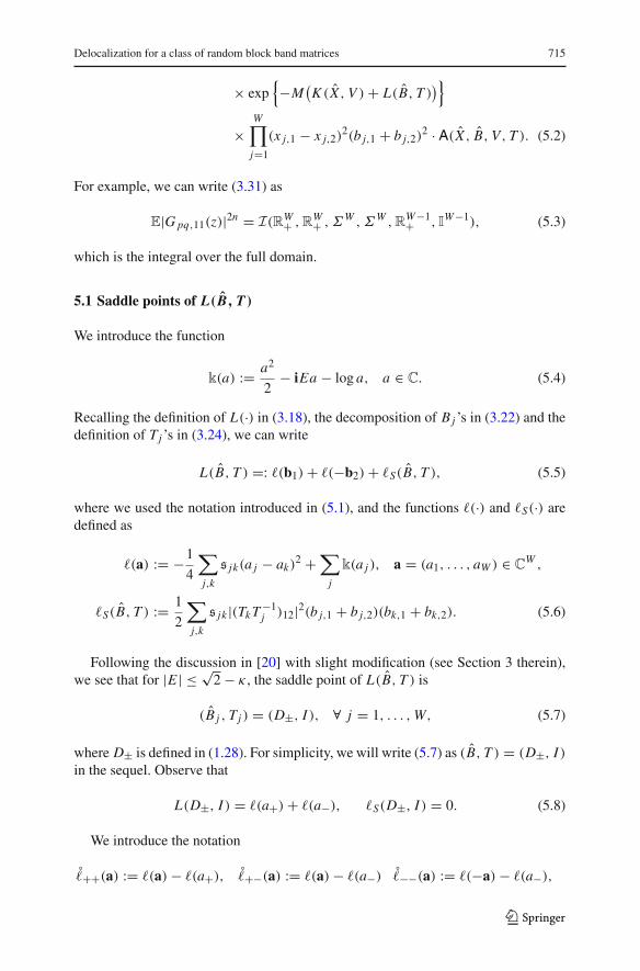
Delocalization for a class of random block band matrices 715
× exp{
−M(
K (X , V )+ L(B, T ))
}
×W∏
j=1
(x j,1 − x j,2)2(b j,1 + b j,2)
2 · A(X , B, V, T ). (5.2)
For example, we can write (3.31) as
E|Gpq,11(z)|2n = I(RW+ ,RW+ ,ΣW ,ΣW ,RW−1+ , IW−1), (5.3)
which is the integral over the full domain.
5.1 Saddle points of L(B, T )
We introduce the function
k(a) := a2
2− iEa − log a, a ∈ C. (5.4)
Recalling the definition of L(·) in (3.18), the decomposition of Bj ’s in (3.22) and thedefinition of Tj ’s in (3.24), we can write
L(B, T ) =: �(b1)+ �(−b2)+ �S(B, T ), (5.5)
where we used the notation introduced in (5.1), and the functions �(·) and �S(·) aredefined as
�(a) := −1
4
∑
j,k
s jk(a j − ak)2 +
∑
j
k(a j ), a = (a1, . . . , aW ) ∈ CW ,
�S(B, T ) := 1
2
∑
j,k
s jk |(TkT−1j )12|2(b j,1 + b j,2)(bk,1 + bk,2). (5.6)
Following the discussion in [20] with slight modification (see Section 3 therein),we see that for |E | ≤ √
2 − κ , the saddle point of L(B, T ) is
(B j , Tj ) = (D±, I ), ∀ j = 1, . . . ,W, (5.7)
where D± is defined in (1.28). For simplicity, we will write (5.7) as (B, T ) = (D±, I )in the sequel. Observe that
L(D±, I ) = �(a+)+ �(a−), �S(D±, I ) = 0. (5.8)
We introduce the notation
�++(a) := �(a)− �(a+), �+−(a) := �(a)− �(a−) �−−(a) := �(−a)− �(a−),
123

716 Z. Bao, L. Erdos
(5.9)
where �(a+) represents the value of �(a) at the point a = (a+, . . . , a+), and �(a−) isdefined analogously. Correspondingly, we adopt the notation
L(B, T ) := L(B, T )− L(D±, I ) = �++(b1)+ �−−(b2)+ �S(B, T ), (5.10)
where the second step is implied by (5.5), (5.8) and (5.9). Now, for each j = 1, . . . ,W ,we deform the contours of b j,1 and b j,2 to
b j,1 ∈ Γ := {ra+|r ∈ R+}, b j,2 ∈ Γ = {−ra−|r ∈ R+} (5.11)
to pass through the saddle points of B-variables, based on the following lemma whichwill be proved in Sect. 7.
Lemma 5.1 With the notation introduced in (5.2), we have
I(
Γ W , Γ W ,ΣW ,ΣW ,RW−1+ , IW−1) = I(
RW+ ,RW+ ,ΣW ,ΣW ,RW−1+ , IW−1)
= E|Gpq,11(z)|2n .
We introduce the notation
r j,1 = |b j,1|, r j,2 = |b j,2|, j = 1, . . . ,W. (5.12)
Along the new contours, we have the following lemma.
Lemma 5.2 Suppose that |E | ≤ √2 − κ . Let b1 ∈ Γ W ,b2 ∈ Γ W . We have
ReL(B, T ) ≥ c∑
a=1,2
W∑
j=1
(
(r j,a − 1)2 + (r j,a − log r j,a − 1))+ Re�S(B, T )
≥ c∑
a=1,2
W∑
j=1
(r j,a − 1)2 (5.13)
for some positive constant c.
Proof Since |E | ≤ √2 − κ , we have Re(b j,1 + b j,2)(bk,1 + bk,2) ≥ 0 for b1 ∈ Γ W
and b2 ∈ Γ W , thus Re�S(B, T ) ≥ 0, in light of the definition in (5.6). Consequently,according to (5.10), it suffices to prove
Re�++(b1)+ Re�−−(b2) ≥ c∑
a=1,2
W∑
j=1
(
(r j,a − 1)2 + (r j,a − log r j,a − 1))
(5.14)
123

Delocalization for a class of random block band matrices 717
for some positive constant c. To see this, we observe the following identities obtainedvia elementary calculation,
Re�++(b1) = E2 − 2
4
(1
2
∑
j,k
s jk(r j,1 − rk,1)2 −
∑
j
(r j,1 − 1)2)
+W∑
j=1
(
r j,1 − log r j,1 − 1)
(5.15)
which together with |E | ≤ √2 − κ and (1.5) implies (5.14) immediately. The same
identity holds if we replace �++(b1) and r j,1’s by �−−(b2) and r j,2’s in (5.15), respec-tively. Hence, we completed the proof of Lemma 5.2. ��
5.2 Saddle points of K (X, V )
Analogously, recalling the definition in (5.6), we can write
K (X , V ) =: −�(x1)− �(x2)+ �S(X , V ), (5.16)
where �(·) is defined in the first line of (5.6) and �S(X , V ) is defined as
�S(X , V ) = 1
2
∑
j,k
s jk |(VkV ∗j )12|2(x j,1 − x j,2)(xk,1 − xk,2). (5.17)
Analogously to the notation L(D±, I ), we will use K (D±, I ) to represent the valueof K (X , V ) at (X j , Vj ) = (D±, I ) for all j = 1, . . . ,W . In addition, K (D+, I ) andK (D−, I ) are defined in the same manner. Observing that
�S(D±, I ) = �S(D+, I ) = �S(D−, I ) = 0, (5.18)
we have
K (D±, I ) = −�(a+)− �(a−), K (D+, I ) = −2�(a+), K (D−, I ) = −2�(a−).(5.19)
Moreover, we employ the notation
K (X , V ) = K (X , V )− K (D±, I ) = −�++(x1)− �+−(x2)+ �S(X , V ). (5.20)
We will need the following elementary observations that are easy to check from (5.19)and (5.6)
K (D±, I )+ L(D±, I ) = 0, ReK (D+, I ) = ReK (D−, I ) = ReK (D±, I ).(5.21)
123

718 Z. Bao, L. Erdos
In addition, we introduce the W × W matrix
Sv = (svjk), svjk := s jk |(VkV ∗j )12|2, (5.22)
and the 2W × 2W matrices
S = S ⊕ S, Sv := S +
(−Sv Sv
Sv −Sv
)
, (5.23)
where Sv depends on the V -variables according to (5.22). Here we regard V -variablesas fixed parameters. Due to the fact |(VkV ∗
j )12| ∈ I, it is easy to see thatSv is aweightedLaplacian of a graph with 2W vertices. In particular, Sv ≤ 0. By the definition (5.22),one can see that Svi i = 0 for all i = 1, . . . ,W . Consequently, we can obtain
∑
k �= j
Svjk =
∑
k �= j
Svk j = −S
vj j =
{−s j j , if j = 1, . . .W−s j−W, j−W , if j = W + 1, . . . , 2W.
Similarly to (1.5), we get
I + Sv ≥ c0 I, (5.24)
where c0 is the constant in Assumption 1.1 (ii). Moreover, it is not difficult to see fromthe definitions in (5.17), (5.22) and (5.23) that
1
4
∑
j,k
s jkT r(X j − Xk)2 + �S(X , V ) = −1
2x′Svx, (5.25)
where we used the notation x := (x′1, x
′2)
′. Now let
ϑ j = arg x j,1, ϑW+ j = arg x j,2, ∀ j = 1, . . . ,W. (5.26)
Then, recalling the parametrization of Vj ’s in (3.25), we have the following lemma.
Lemma 5.3 Assume that x j,1, x j,2 ∈ Σ for all j = 1, . . . ,W. We have
ReK (X , V ) ≥ 1
4
2W∑
j,k=1
(Sv) jk(cosϑ j − cosϑk)2 + c
2W∑
j=1
(
sin ϑ j − E
2
)2(5.27)
for some positive constant c. In addition, ReK (X , V ) attains its minimum 0 at thefollowing three types of saddle points
– Type I : For each j , X j = D± or D∓, θ j ∈ L v j = 0 if X j = X1, andv j = 1 if X j �= X1,
– Type II : For each j , X j = D+, Vj ∈ U (2),– Type III : For each j , X j = D−, Vj ∈ U (2),
123
Delocalization for a class of random block band matrices 719
which are the restrictions of three types of saddle points in Sect. 4.1, on X and V -variables.
Remark 5.4 The Type I saddle points of (X , V ) are exactly those points satisfying
V ∗j X j V j = D±, ∀ j = 1, . . . ,W, or V ∗
j X j V j = D∓, ∀ j = 1, . . . ,W.
In Lemma 5.3, we wrote them in terms of X j , v j and θ j in order to evoke the para-meterization in (3.23) and (3.25).
Proof By (5.16), (5.25), the definitions of the functions �(·) in (5.7) and k(·) in (5.4),we can write
K (X , V ) = −1
2x∗Svx −
W∑
j=1
(
k(x j,1)+ k(x j,2)− k(a+)− k(a−))
.
By using (5.26) and the fact |x j,a | = 1 for all j = 1, . . . ,W and a = 1, 2, we canobtain via elementary calculation
ReK (X , V ) = 1
4
2W∑
j,k=1
(Sv) jk
(
(cosϑ j − cosϑk)2 − (sin ϑ j − sin ϑk)
2)
+2W∑
j=1
(
sin ϑ j − E
2
)2. (5.28)
In light of the fact Sv ≤ 0 and (5.24), we have
I + 1
2Sv ≥ I + S
v ≥ c0 I. (5.29)
Applying (5.29) to the r.h.s. of (5.28) yields (5.27).Then what remains is to show thatReK (X , V ) attains its minimum 0 at three types
of points listed in Lemma 5.3. This step can be verified in the same manner as thecounterpart in [20]. Hence, we just omit it here and refer to the proof of Lemma 2 in[20] for more details. Therefore, we completed the proof of Lemma 5.3. ��
5.3 Vicinities of the saddle points
Having studied the saddle points of L(B, T ) and K (X , V ), we then introduce somesmall vicinities of them. To this end, we introduce the quantity
Θ ≡ Θ(N , ε0) := WN ε0 (5.30)
123
720 Z. Bao, L. Erdos
for small positive constant ε0 which will be chosen later. Let a = (a1, . . . , aW ) ∈ CW
be any complex vector. In the sequel, we adopt the notation for any d ∈ C,
a + d := (a1 + d, . . . , aW + d), da := (da1, . . . , daW ),arg(a) := ( arg(a1), . . . , arg(aW )
)
. (5.31)
Now, we define the domains Υ b+, Υ b−, Υ x+, Υ x− and ΥS as follows
Υ b± ≡ Υ b±(N , ε0) :={
a ∈ Γ W : ||a − a±||22 ≤ Θ
M
}
,
Υ x± ≡ Υ x±(N , ε0) :={
a ∈ ΣW : || arg(a−1± a)||22 ≤ Θ
M
}
,
ΥS ≡ ΥS(N , ε0) :={
a ∈ RW−1+ : −a′S(1)a ≤ Θ
M
}
, (5.32)
where the superscripts b and x indicate that these will be domains of the correspondingvariables. In order to define the vicinities of the Type I saddle points properly, weintroduce the permutation ε j of {1, 2}, for each triple (x j,1, x j,2, v j ). Specifically,
recalling the fact of u j =√
1 − v2j from (3.25), we define
v j,ε j ≡ v j,ε j (ε1) := v j1(ε j = ε1)+ u j1(ε j �= ε1).Denoting by ε = (ε1, . . . , εW ) and ε(a) = (ε1(a), . . . , εW (a)) for a = 1, 2, we set
xε(a) = (x1,ε1(a), . . . , xW,εW (a)), a = 1, 2, vε = (v2,ε2 , . . . , vW,εW ). (5.33)
With this notation, we now define the Type I, II, and III vicinities, parameterizedby (b1,b2, x1, x2, t, v) of the corresponding saddle point types. We also define thespecial case of the Type I vicinity, namely, Type I’ vicinity, corresponding to the TypeI’ saddle point defined in Sect. 4.1.
Definition 5.5 – Type I vicinity :(
b1,b2, xε(1), xε(2), t, vε
) ∈ Υ b+ × Υ b− × Υ x+ ×Υ x− × ΥS × ΥS for some ε.
– Type I’ vicinity :(
b1,b2, x1, x2, t, v) ∈ Υ b+ × Υ b− × Υ x+ × Υ x− × ΥS × ΥS .
– Type II vicinity :(
b1,b2, x1, x2, t, v) ∈ Υ b+ × Υ b− × Υ x+ × Υ x+ × ΥS × I
W−1.– Type III vicinity :
(
b1,b2, x1, x2, t, v) ∈ Υ b+ × Υ b− × Υ x− × Υ x− × ΥS × I
W−1.
In the following discussion, the parameter ε0 in Θ is allowed to be different fromline to line. However, given ε1 in (1.8), we shall always choose ε2 in (1.16) and ε0 in(5.30) according to the rule
Cε2 ≤ ε0 ≤ ε1/C (5.34)
for some sufficiently large C > 0. Consequently, by Assumption 1.14 we have
N (log N )−10 ≥ M = M1−4ε0M4ε0 ≥ W (4+2γ+ε1)(1−4ε0)M4ε0
123

Delocalization for a class of random block band matrices 721
� W (4+2γ+4ε0)M4ε0 = W 2γΘ4. (5.35)
To prove Theorem 1.15, we split the task into three steps. The first step is to excludethe integral outside the vicinities. Specifically, we will show the following lemma.
Lemma 5.6 Under Assumptions 1.1 and 1.14, we have,
I(
Γ W , Γ W ,ΣW ,ΣW ,RW−1+ , IW−1)
= 2WI(
Υ b+, Υ b−, Υ x+, Υ x−, ΥS, ΥS)+ I
(
Υ b+, Υ b−, Υ x+, Υ x+, ΥS, IW−1)
+ I(
Υ b+, Υ b−, Υ x−, Υ x−, ΥS, IW−1)+ O(e−Θ). (5.36)
Remark 5.7 The first three terms on the r.h.s. of (5.36) correspond to the integrals overvicinities of the Type I, II, and III saddle points, respectively. Note that for the firstterm, we have used the fact that the total contribution of the integral over the Type Ivicinity is 2W times that over the Type I’ vicinity.
The second step, is to estimate the integral over the Type I vicinity. We have thefollowing lemma.
Lemma 5.8 Under Assumptions 1.1 and 1.14, there exists some positive constant C0uniform in n and some positive number N0 = N0(n) such that for all N ≥ N0,
2W∣
∣I(Υ b+, Υ b−, Υ x+, Υ x−, ΥS, ΥS)∣
∣ ≤ NC0
(Nη)n. (5.37)
The last step is to show that the integral over the Type II and III vicinities are alsonegligible.
Lemma 5.9 Under Assumptions 1.1 and 1.14, there exists some positive constant csuch that,
I(
Υ b+, Υ b−, Υ x+, Υ x+, ΥS, IW−1) = O
(
e−cW)
,
I(
Υ b+, Υ b−, Υ x−, Υ x−, ΥS, IW−1) = O(e−cW ).
Therefore, the remaining task is to prove Lemmas 5.1, 5.6, 5.8 and 5.9. For theconvenience of the reader,weoutline the organization of the subsequent part as follows.
At first, the proofs of Lemmas 5.1 and 5.6 require a discussion on the bound ofthe integrand, especially on the term A(·), which contains the integral over all theGrassmann variables. To this end, we perform a crude analysis for the function A(·)in Sect. 6 in advance, with which we are able to prove Lemmas 5.1 and 5.6 in Sect. 7.Then, we can restrict ourselves to the integral over the vicinities, i.e., prove Lemmas5.8 and 5.9. In Sect. 8, we will analyze the factor exp{−M(K (X , V ) + L(B, T ))},which is approximately Gaussian in the Type I vicinity. The key step is to deformthe contours of X and B-variables again to the steepest paths exactly, whereby wecan control the error terms in the integrand and prove Lemma 5.8 in Sect. 9. In the
123

722 Z. Bao, L. Erdos
Type II and III vicinities, we only deform the contours of B-variables again and boundexp{−MK (X , V )} by its absolute value directly. It turns out to be enough for ourproof of Lemma 5.9, which is given in Sect. 10.
6 Crude bound on A(X, B, V, T )
In this section, we provide a bound on the functionA(·) in terms of the B, T -variables,which holds on all the domains under discussion in the sequel. Here, by crude boundwe mean a bound of order exp{O(WN ε2)}), which will be specified in Lemma 6.1below. By the definition in (3.32), we see that A(·) is an integral of the product ofQ(·),P(·) andF(·). As mentioned in Sect. 4.2, a typical procedure we will adopt is toignoreQ(·) at first, then estimate the integrals of P(·) and F(·), which are denoted byP(·) and F(·), respectively [see (4.2) and (4.3)], finally, we make necessary commenton how to modify the bounding scheme to take Q(·) into account, whereby we canget the desired bound for A(·).
For the sake of simplicity, from now on, we will use the notation
ω j,1 := ω j,11, ω j,2 := ω j,12, ω j,3 := ω j,21, ω j,4 := ω j,22,
ξ j,1 := ξ j,11, ξ j,2 := ξ j,21, ξ j,3 := ξ j,12, ξ j,4 := ξ j,22. (6.1)
Moreover, we introduce the domains
Σ :={
reiϑ : |r − 1| ≤ 1
10, ϑ ∈ L
}
,
K ≡ K(E) :=
⎧
⎪
⎪
⎨
⎪
⎪
⎩
{
ω ∈ C : 0 ≤ argω ≤ arg a+2 + π
8
}
, if E ≥ 0,
{
ω ∈ C : arg a+2 − π
8 ≤ argω ≤ 0}
, if E < 0.
(6.2)
By the assumption that |E | ≤ √2−κ in (1.16), it is easy to see that | argω| ≤ π/4−c
for all ω ∈ K ∪ K, where c is some positive constant depending on κ . Our aim is toshow the following lemma.
Lemma 6.1 Suppose thatb1,b2, x1, x2 ∈ KW×K
W×ΣW×ΣW .Under the assump-tion of Theorem 1.15, we have
|A(X , B, V, T )| ≤ eO(WN ε2 )W∏
j=1
(
r−1j,1 + r−1
j,2 + t j + 1)C := eO(WN ε2 )p(r−1, t).
Remark 6.2 Obviously, using the terminology introduced at the end of Sect. 3.6, wehave
p(r−1, t) ∈ Q
(
{
r−1j,1 , r
−1j,2 , t j
}W
j=1; κ1, κ2, κ3
)
, κ1 = eO(W ), κ2, κ3 = O(1).
(6.3)
123

Delocalization for a class of random block band matrices 723
6.1 Integral of Q
In this section, we investigate the function
Q(Ω,Ξ, P1, Q1, X[1], y[1],w[1])
:=∫
dω[1]dξ [1] Q(Ω,Ξ,ω[1], ξ [1], P1, Q1, X[1], y[1],w[1]). (6.4)
RecallQdeg(a; κ1, κ2, κ3) defined at the end of Sect. 3.6, the parameterization in (3.15)and (3.25) and the notation introduced in (6.1). We have the following lemma.
Lemma 6.3 If we regard σ, v[1]p , v[1]q , P1 and (X [1])−1-entries as fixed parameters,
we have
Q(·) ∈ Qdeg(S; κ1, κ2, κ3), κ1 = WO(1), κ2, κ3 = O(1), (6.5)
where S is the set of variables defined by
S :={
t, s, (y[1]k )
−1, eiσ [1]k , e−iσ [1]
k ,ωi,aξ j,b
M
}
i, j=1,...,W ;k=p,q;a,b=1,...,4
.
Proof Note thatQ(·) can be regarded as a function of the Grassmann variables in ω[1]and ξ [1]. Hence, by the definition in (3.30), it is a polynomial of these variables withbounded degree. In addition, we can always combine the factor 1/
√M with Ω j and
Ξ j -variables in the first factor of the r.h.s. of (3.30). Then it is not difficult to checkthat
Q(·) ∈ Qdeg(S′; κ1, κ2, κ3), κ1 = WO(1), κ2, κ3 = O(1), (6.6)
where
S′ :={
t, s,(
y[1]k
)−1, eiσ [1]
k , e−iσ [1]k ,ω j,rξ
[1]k,b√
M,ξ j,rω
[1]k,b√
M, ω
[1]k,aξ
[1]�,b
}
j=1,...,W ;k=p,q;r=1,...,4;a,b=1,2
.
By the definition in (6.4), Q(·) is the integral ofQ(·) over the ω[1] and ξ [1]-variables.Now, we regard all the other variables in S′, except ω[1] and ξ [1]-variables, as para-meters. By the definition of Grassmann integral, we know that only the coefficient ofthe highest order term
∏
k=p,q∏
a=1,2 ω[1]k,aξ
[1]k,a inQ(·) survives after integrating ω[1]
and ξ [1]-variables out. Then, it is easy to see (6.5) from (6.6), completing the proof.��
123
724 Z. Bao, L. Erdos
6.2 Integral of P
In this subsection, we temporarily ignore the Ω and Ξ -variables from Q(·), andestimate P(X , B, V, T ) defined in (4.2). Recalling r j,1 and r j,2 defined in (5.12), wecan formulate our estimate as follows.
Lemma 6.4 Suppose that the assumptions in Lemma 6.1 hold. We have
|P(X , B, V, T )| ≤ eO(W )W∏
j=1
(
r−1j,1 + r−1
j,2 + t j + 1)O(1)
. (6.7)
Proof We start with one factor from P(·) (see (3.29)), namely
� j := 1
detM(
1 + M−1V ∗j X
−1j V jΩ j T
−1j B−1
j TjΞ j)
= exp{
− M log det(
1 + M−1V ∗j X
−1j V jΩ j T
−1j B−1
j TjΞ j)
}
= 1 +4∑
�=1
1
M�−1 p�(X j , B j , Vj , Tj ,Ω j , Ξ j ). (6.8)
Here p�(·) is a polynomial in X−1j , B
−1j , Vj , Tj ,Ω j and Ξ j -entries with bounded
degree and bounded coefficients. Moreover, if we regard p�(·) as a polynomial ofΩ j and Ξ j -entries, it is homogeneous, with degree 2�, and the total degree for Ω j -variables is �, thus that for Ξ j -entries is also �. More specifically, we can write
p�(X j , B j , Vj , Tj ,Ω j , Ξ j ) =4∑
α1,...,α�,β1,...,β�=1
p�,α,β(X j , B j , Vj , Tj )
�∏
i=1
ω j,αi ξ j,βi ,
where we used the notation in (6.1) and denoted α = (α1, . . . , α�) and β =(β1, . . . , β�). It is easy to verify that� j is of the form (6.8) by taking Taylor expansionw.r.t. the Grassmann variables. The expansion in (6.8) terminates at � = 4, owing tothe fact that there are totally 8 Grassmann variables from Ω j and Ξ j . In addition, itis also easy to check that p�,α,β(·) is a polynomial of X−1
j , B−1j , Vj , Tj -entries with
bounded degree and bounded coefficients, which implies that there exist two positiveconstants C1 and C2, such that
|p�,α,β(·)| ≤ C1
(
r−1j,1 + r−1
j,2 + t j + 1)C2
(6.9)
uniformly in �,α and β. Here we used the fact that X−1j and Vj -entries are all bounded
and Tj -entries are bounded by 1 + t j .Now,we go back to the definition ofP(·) in (3.29) and study the last factor. Similarly
to the discussion above, it is easy to see that for k = p or q,
� k := det(
V ∗k XkVk + M−1ΩkT
−1k B−1
k TkΞk)
det Bk= p0(Xk, Bk)
123
Delocalization for a class of random block band matrices 725
+4∑
�=1
∑
α,β
p�,α,β(Xk, Bk, Vk, Tk)�∏
i=1
ωk,αk,i ξk,βk,i , (6.10)
where p0(·) = det Xk/ det Bk and p�,α,β(·)’s are some polynomials of Xk, B−1k ,
Vk, Tk-entries with bounded degree and bounded coefficients. Similarly, we have
|p0(·)|, |p�,α,β(·)| ≤ C1(r−1k,1 + r−1
k,2 + tk + 1)C2 (6.11)
for some positive constants C1 and C2.According to the definitions in (6.8) and (6.10), we can rewrite (3.29) as
P(Ω,Ξ, X , B, V, T ) = exp
⎧
⎨
⎩
−∑
j,k
s jkT rΩ jΞk
⎫
⎬
⎭
W∏
j=1
� j
∏
k=p,q
� k . (6.12)
In light of the discussion above,∏W
j=1 � j∏
k=p,q � k is a polynomial of X−1, B−1,
V, T,Ω and Ξ -entries, in which each monomial is of the form
q�,α,β(X−1, B−1, V, T )
W∏
j=1
� j∏
i=1
ω j,α j,i ξ j,β j,i , (6.13)
where we used the notation
� = (�1, . . . , �W ), α ≡ α(�) = (α1, . . . ,αW ), β ≡ β(�) = (β1, . . . ,βW ),
α j = (α j,1, . . . , α j,� j ), β j = (β j,1, . . . , β j,� j ), (6.14)
and q�,α,β(·) is a polynomial of X , X−1, B−1, V and T -entries. Moreover, all theentries of �,α and β are bounded by 4. By (6.9) and (6.11), we have
|q�,α,β(X−1, B−1, V, T )| ≤ eO(W )
W∏
j=1
(
r−1j,1 + r−1
j,2 + t j + 1)C. (6.15)
In addition, it is easy to see that the number of the summands of the form (6.13) in∏W
j=1 � j∏
k=p,q � k is bounded by eO(W ).Now, we define the vectors
� := (ω1,ω2,ω3,ω4), � := (ξ1, ξ2, ξ3, ξ4), (6.16)
where ωα = (ω1,α, . . . , ωW,α) and ξα = (ξ1,α, . . . , ξW,α) for α = 1, 2, 3, 4. Here weused the notation (6.1). In addition, we introduce the matrix
˜H = ˜S ⊕˜S ⊕˜S ⊕˜S.
123

726 Z. Bao, L. Erdos
It is easy to check∑
j,k s jkT rΩ jΞk = �˜H�′. By using theGaussian integral formulafor the Grassmann variables (3.2), we see that for each �,α and β, we have
∣
∣
∣
∫
dΩdΞ · exp⎧
⎨
⎩
−∑
j,k
s jkT rΩ jΞk
⎫
⎬
⎭
·W∏
j=1
� j∏
i=1
ω j,α j,i ξ j,β j,i
∣
∣
∣ ≤ | det˜H(I|J)|,
(6.17)
for some index sets I and J with |I| = |J|. By Assumption 1.1 (i) and (ii), we see thatthe 2-norm of each row of˜S is O(1). Consequently, by using Hadamard’s inequality,we have
| det˜H(I|J)| = eO(W ). (6.18)
Therefore, (6.12)–(6.18) and the bound eO(W ) for the total number of summands ofthe form (6.13) in
∏Wj=1 � j
∏
k=p,q � k imply (6.7). Thus we completed the proof.��
6.3 Integral of F
In this subsection, we also temporarily ignore the X [1], y[1],w[1], P1, Q1-variablesfromQ(·), and estimateF(X , B, V, T ) defined in (4.3).We have the following lemma.
Lemma 6.5 Suppose that the assumptions in Lemma 6.1 hold. We have
|F(X , B, V, T )| ≤ eO(WN ε2 )∏
k=p,q
(
r−1k,1 + r−1
k,2 + tk + 1)O(1)
. (6.19)
Proof Recalling the decomposition of F(·) in (3.19) together with the parameteriza-tion in (3.29), we will study the integrals
G(B, T ) :=∫
dν(Q1)dy[1]dw[1] g(Q1, T, B, y[1],w[1]), (6.20)
F(X , V ) :=∫
dμ(P1)dX[1] f (P1, V, X , X
[1]) (6.21)
separately. Recalling the convention at the end of Sect. 3, we use f (·) and g(·) torepresent the integrands above. One can refer to (3.20) and (3.21) for the definition.From the assumption η ≤ M−1N ε2 , we see
|F(X , V )| ≤ eO(WN ε2 ), (6.22)
since P1, V, X , X [1]-variables are all bounded and | det X [1]p |, | det X [1]
q | ∼ 1 whenx1, x2 ∈ Σ .
123
Delocalization for a class of random block band matrices 727
For G(B, T ), we use the facts
Re(Tr B jY[1]k J ) ≥ 0, Re(iTrY [1]
k J Z) = −ηTrY [1]k ≤ 0,
TrY [1]k JY [1]
� J ≥ 0, k, � = p, q,∣
∣
(
w[1]q (w
[1]q )
∗)12
∣
∣ ≤ 1,∣
∣
(
w[1]p (w
[1]p )
∗)21
∣
∣ ≤ 1, (6.23)
to estimate trivially several terms, whereby we can get the bound
|g(·)| ≤ exp{
−Mη∑W
j=1 TrRe(Bj )J}
∏
k=p,q
(
y[1]k
)n+3exp
{
− skkT rRe(Bk)Y[1]k J
}
.
(6.24)
Here Re(Bj ) = Q−11 T−1
j Re(B j )Tj Q1. Hence, integrating y[1]p and y[1]
q out yields
∫
R2+dy[1]
p dy[1]q |g(Q1, T, B, y[1],w[1])| ≤ C
exp{
− Mη∑W
j=1 TrRe(Bj )J}
∏
k=p,q
(
(
w[1]k
)∗JRe(Bk)w
[1]k
)C1,
(6.25)
for some positive constants C and C1 depending on n, where we used the elementaryfacts that skk ≥ c for some positive constant c and
TrRe(Bj )Y[1]k J = y[1]
k
(
w[1]k
)∗JRe(Bj )w
[1]k , k = p, q, j = 1, . . . ,W.
(6.26)
Now, note that
(w[1]k )
∗ JReBjw[1]k ≥ λ1(JReBj ), k = p, q, j = 1, . . . ,W. (6.27)
In addition, it is also easy to see λ1(Tj ) = s j − t j and λ1(Q1) = s − t , according tothe definitions in (3.25). Now, by the fact J A−1 = AJ for any A ∈ U (1, 1), we have
JReBj = Q1Tjdiag(
Reb j,1,Reb j,2)
Tj Q1. (6.28)
Consequently, we can get
λ1(JReBj ) ≥ (s j − t j )2(s − t)2min{Reb j,1,Reb j,2} = min{Reb j,1,Reb j,2}
(s j + t j )2(s + t)2,
(6.29)
123

728 Z. Bao, L. Erdos
by recalling the facts s2− t2 = 1 and s2j − t2j = 1. Therefore, combining (6.25), (6.27)and (6.29), we have
∫
R2+dy[1]
p dy[1]q |g(·)| ≤ C(s + t)4C1 exp
⎧
⎨
⎩
−MηW∑
j=1
Tr(ReBj )J
⎫
⎬
⎭
×∏
k=p,q
(sk + tk)2C1
(
min{Rebk,1,Rebk,2})C1. (6.30)
Now, what remains is to estimate the exponential function in (6.30). By elementarycalculation from (6.28) we obtain
Tr(ReBj )J ≥ (Reb j,1 + Reb j,2)(
(s2j + t2j )(s2 + t2)− 4sts j t j
)
.
Observe that
(
s2j + t2j
)
(s2 + t2)− 4sts j t j =(
s2j + t2j
)2(s2 + t2)2 − 16(sts j t j )2
(
s2j + t2j
)
(s2 + t2)+ 4sts j t j
≥ 4t4 + 4t2 + 4t4j + 4t2j + 1
2(
1 + 2t2j
)
(1 + 2t2)≥ 1 + 2t2
2(1 + 2t2j ).
It implies that
exp
⎧
⎨
⎩
−MηW∑
j=1
Tr(ReBj )J
⎫
⎬
⎭
≤ exp
⎧
⎨
⎩
−cMηW∑
j=1
r j,1 + r j,21 + 2t2j
(1 + 2t2)
⎫
⎬
⎭
, (6.31)
for some positive constant c, where we have used the fact Reb j,α ≥ cr j,α for allj = 1, . . . ,W and α = 1, 2, in light of the assumption |E | ≤ √
2 − κ and thedefinition ofK in (6.2). Plugging (6.31) into (6.30), estimating (s + t)2 ≤ 2(1+ 2t2),and integrating t out, we can crudely bound
∫
R2+dy[1]
p dy[1]q
∫
R+2tdt · |g(·)| ≤ C
(
1
Mη
)C2
⎛
⎝
W∑
j=1
r j,1 + r j,21 + 2t2j
⎞
⎠
−C2
×∏
k=p,q
(
1 + 2t2kmin{rk,1, rk,2}
)C1
. (6.32)
123
Delocalization for a class of random block band matrices 729
Now, we use the trivial bounds
⎛
⎝
W∑
j=1
r j,1 + r j,21 + 2t2j
⎞
⎠
−C2
≤(
1 + 2t2prp,1 + rp,2
)C2
≤(
(1 + 2t2p)(
r−1p,1 + r−1
p,2
))C2,
(6.33)
and
1 + 2t2kmin{rk,1, rk,2} ≤ C(1 + 2t2k )
(
r−1k,1 + r−1
k,2
)
. (6.34)
Inserting (6.33) and (6.34) into (6.32) and integrating out the remaining variablesyields
|G(B, T )| ≤ C
(
1
Mη
)C1∏
k=p,q
(
r−1k,1 + r−1
k,2 + tk + 1)C3. (6.35)
Combining (6.22) and (6.35) we can get the bound (6.19). Thus we completed theproof of Lemma 6.5. ��
6.4 Summing up: Proof of Lemma 6.1
In the discussions in Sects. 6.2 and 6.3, we ignored the irrelevant factorQ(·). However,it is easy to modify the discussion slightly to take this factor into account, wherebywe can prove Lemma 6.1.
Proof At first, by the definition in (6.4), we can rewrite (3.32) as
A(·) =∫
dX [1]dy[1]dw[1]dΩdΞdμ(P1)dν(Q1) P(·)Q(·)F(·).
Now, by the conclusion κ1 = WO(1) in Lemma 6.3, it suffices to consider one term inQ(·), which is a monomial of the form p(t, s, (y[1]
p )−1, (y[1]
q )−1)q(Ω,Ξ), regarding
σ, v[1]p , v
[1]q , P1-variables, X [1]-variables and w[1]-variables as bounded parameters.
Here p(·) is a monomial of t, s, (y[1]p )
−1, (y[1]q )
−1 and q(·) is a monomial of Ω,Ξ -variables, both with bounded coefficients and bounded degrees, according to the factκ2, κ3 = O(1) in Lemma 6.3. Now we define
Pq(X , B, V, T ) :=∫
dΩdΞ P(·) · q(Ω,Ξ),
Fp(X , B, V, T ) :=∫
dX [1]dy[1]dw[1]dμ(P1)dν(Q1) F(·)
· p(
t, s, (y[1]p )
−1, (y[1]q )
−1)
. (6.36)
123

730 Z. Bao, L. Erdos
By repeating the discussions in Sects. 6.2 and 6.3 with slight modification, we caneasily see that (6.7) and (6.19) hold as well, if we replace P(·) and F(·) by Pq(·) andFp(·), respectively. Therefore, we completed the proof of Lemma 6.1. ��
7 Proofs of Lemmas 5.1 and 5.6
In this section, with the aid of Lemma 6.1, we prove Lemmas 5.1 and 5.6. A keyproblem is that the domain of t-variables is not compact. This forces us to analyze theexponential function
M(t) := exp{
− MRe(
�S(B, T ))
}
(7.1)
carefully for any fixed B-variables. Recall the definition of the sector K in (6.2). Forb1 ∈ K
W and b2 ∈ KW , we have
minj,k
Re(b j,1 + b j,2)(bk,1 + bk,2) ≥ cminj,k
∑
a,b=1,2
r j,ark,b ≥ cminj,a
r2j,a := A(B),
(7.2)
From now on, we regard M(t) as a measure of the t-variables and study it in thefollowing two regions separately:
(i) : t ∈ IW−1, (i i) : t ∈ R
W−1+ \ IW−1.
Roughly speaking, when t ∈ IW−1, we will see thatM(t) can be bounded pointwisely
by a Gaussian measure. More specifically, we have the following lemma.
Lemma 7.1 With the notation above, we have
M(t) ≤ exp
⎧
⎨
⎩
−M
12A(B)
∑
j,k
s jk(tk − t j )2
⎫
⎬
⎭
, ∀ t ∈ IW−1.
Proof Using the definition of �S(B, T ) in (5.6) and A(B) in (7.2) and the fact|(TkT−1
j )12| = |s j tkeiσk − skt j eiσ j |, we have
Re�S(B, T ) ≥ 1
2A(B)
∑
j,k
s jk
∣
∣
∣s j tkeiσk − skt j e
iσ j∣
∣
∣
2. (7.3)
Simple estimate using s2j = 1 + t2j shows that
∣
∣
∣s j tkeiσk − skt j e
iσ j∣
∣
∣
2 ≥ 1
4(tk − t j )
2
(
1
1 + 2t2j+ 1
1 + 2t2k
)
≥ 1
6(tk − t j )
2.
123

Delocalization for a class of random block band matrices 731
(7.4)
Notice that the assumption t ∈ IW−1 was used only in the last inequality. By (7.3),
(7.4) and the definition (7.1), Lemma 7.1 follows immediately. ��However, the behavior of M(t) for t ∈ R
W−1+ \IW−1 is much more sophisticated.We will not try to provide a pointwise control ofM(t) in this region. Instead, we willbound the integral of q(t) againstM(t) over this region, for any given monomial q(·)of interest. More specifically, recalling the definition of Θ in (5.30) and the spanningtree G0 = (V, E0) in Assumption 1.1, and additionally setting
L := M
4A(B) min
i, j∈E0si j , (7.5)
we have the following lemma.
Lemma 7.2 Let q(t) = ∏Wj=2 t
n jj be a monomial of t-variables, with powers n j =
O(1) for all j = 2, . . . ,W. We have
∫
RW−1+ \IW−1
W∏
j=2
dt j M(t)q(t) ≤(
1 + L− 12
)O(W 2)
exp{
−Θ2A(B)+ O(W 2 log N )}
(7.6)
Remark 7.3 Roughly speaking, byLemma7.2we see that the integral of q(t)-variablesagainst the measureM(t) over the region RW−1+ \ IW−1 is exponentially small, owingto the fact Θ2 � W 2 log N .
We will postpone the proof of Lemma 7.2 to the end of this section. In the sequel,at first, we prove Lemmas 5.1 and 5.6 with the aid of Lemmas 6.1, 7.1 and 7.2. Beforecommencing the formal proofs, we mention two basic facts which are formulated asthe following lemma.
Lemma 7.4 Under Assumption 1.1, we have the following two facts.
– For the smallest eigenvalue of −S(1), there exists some positive constant c suchthat
λ1(−S(1)) ≥ c/W 2. (7.7)
– Let � = (ρ2, . . . , ρW )′ be a real vector and ρ1 = 0. If there is at least one
α ∈ {2, . . . ,W } such that �α ≥ Θ/√M, then we have
∑
j,k
s jk(� j − �k)2 ≥ Θ/M. (7.8)
123

732 Z. Bao, L. Erdos
Proof Let � = (ρ2, . . . , ρW )′ be a real vector and ρ1 = 0. Now, we assume |ρα| =maxβ=2,...,W |ρβ |. Then
−ρ′S(1)ρ||ρ||22
=12
∑
j,k s jk(ρ j − ρk)2∑
j ρ2j
≥ c(ρα − ρ1)2W 2ρ2α
= c
W 2 ,
where the second step follows fromAssumption 1.1 (iv) andCauchy-Schwarz inequal-ity. Analogously, we have
∑
j,k s jk(� j − �k)2 ≥ c�2α/W , which implies (7.8) by thedefinition of Θ in (5.30). Hence, we completed the proof. ��
Recalling the notation defined in (5.2) and the facts |x j,a | = 1 and |b j,a | = r j,a forall j = 1, . . . ,W and a = 1, 2, for any sequence of domains, we have
∣
∣
∣I(Ib1, Ib2, Ix1 , Ix2 , It , Iv)∣
∣
∣
≤ eO(W log N )∫
Ib1
W∏
j=1
db j,1
∫
Ib2
W∏
j=1
db j,2
∫
Ix1
W∏
j=1
dx j,1
∫
Ix2
W∏
j=1
dx j,2
×∫
It
W∏
j=2
2t jdt j
∫
Iv
W∏
j=2
2v jdv j × exp{
−M(
ReK (X , V )+ ReL(B, T ))
}
· |A(X , B, V, T )| ·W∏
j=1
(r j,1 + r j,2)2. (7.9)
In addition, according to Lemma 6.1, we have
|A(X , B, V, T )| ·W∏
j=2
2t j ·W∏
j=2
2v j ·W∏
j=1
(r j,1 + r j,2)2 ≤ eO(WN ε2 )p(r, r−1, t),
(7.10)
for some polynomial p(r, r−1, t) with positive coefficients, and
p(r, r−1, t) ∈ Q(
{r j,1, r j,2, r−1j,1 , r
−1j,2 , t j }Wj=1; κ1, κ2, κ3
)
, κ1 = eO(W ),
κ2, κ3 = O(1). (7.11)
7.1 Proof of Lemma 5.1
At first, since throughout the whole proof, the domains of x1, x2, and v-variables,namely, ΣW ,ΣW and I
W−1, will not be involved, we just use ∗’s to represent them,in order to simplify the notation.
Now, we introduce the following contours with the parameter D ∈ R+,
ΓD := {ra+|r ∈ [0,D]} ⊂ Γ, RD = [0, (Rea+)D] ⊂ R+,
123

Delocalization for a class of random block band matrices 733
LD := {(Rea+)D + i(Ima+)r |r ∈ [0,D]}.
In addition, we recall the sector K defined in (6.2). Then, trivially, we haveR+, Γ,LD ⊂ K and R+, Γ , LD ∈ K for all D ∈ R+.
Observe that the integrand in (5.2) is an analytic function of the B-variables. Tosee this, we can go back to the integral representation (3.17) and the definitions ofL(B) and P(Ω,Ξ, X, B) in (3.18). Since exp{M log det Bj } = (det Bj )
M , actuallythe logarithmic terms in L(B) do not produce any singularity in the integrand in(3.17); it can also compensate the factors b−�
j,a from P(Ω,Ξ, X, B) since � M .Consequently, we have
I(
(ΓD ∪ LD)W , (ΓD ∪ LD)
W , ∗, ∗,RW−1+ , ∗)
= I(
(RD)W , (RD)
W , ∗, ∗,RW−1+ , ∗)
.
Hence, to prove Lemma 5.1, it suffices to prove the following lemma.
Lemma 7.5 Suppose that |E | ≤ √2 − κ . As D → ∞, the following convergence
hold,
(i) : I(
(ΓD ∪ LD)W , (ΓD ∪ LD)
W , ∗, ∗,RW−1+ , ∗)
−I(
(ΓD)W , (ΓD)
W , ∗, ∗,RW−1+ , ∗)
→ 0,
(ii) : I(
(Γ )W , (Γ )W , ∗, ∗,RW−1+ , ∗)
− I(
(ΓD)W , (ΓD)
W , ∗, ∗,RW−1+ , ∗)
→ 0,
(iii) : I(
RW+ ,RW+ , ∗, ∗,RW−1+ , ∗
)
− I(
RWD,R
WD, ∗, ∗,RW−1+ , ∗
)
→ 0.
Proof For simplicity, we use the notation
Ib,1D := (ΓD ∪ LD)W × (ΓD ∪ LD
)W \ (ΓD)W × (ΓD)W ,Ib,2D := Γ W × Γ W \ (ΓD)W × (ΓD)W , Ib,3D := R
W+ × RW+ \ RW
D × RWD.
Now, recall the definition of the function �(a) in (5.6) and the representation of L(B, T )in (5.5). Hence, in light of the definition of M(t) in (7.1), we have
exp{− MReL(B, T )
} = exp{− M
(
Re�(b1)+ Re�(−b2))}
M(t). (7.12)
By the assumption |E | ≤ √2−κ , we see thatReb j,abk,a > 0 for allb j,a, bk,a ∈ K∪K.
Consequently, when b j,1 ∈ K and b j,2 ∈ K for all j = 1, . . . ,W , we have
Re�(b1)+ Re�(−b2) ≥∑
a=1,2
∑
j
(
1
2(1 + s j j )Reb2j,a + (−1)a+1E Imb j,a − log r j,a
)
≥ c∑
j
(
r2j,1 + r2j,2
)
−∑
j
(log r j,1 + log r j,2), (7.13)
where we used Assumption 1.1 (ii) and the fact that (−1)a+1E Imb j,a ≥ 0.
123

734 Z. Bao, L. Erdos
Now, when (b1,b2) ∈ Ib,iD for i = 1, 2, 3, we have∑
a=1,2∑
j r2j,a ≥ cD2 for
some positive constant c, which implies the trivial fact
∑
j
(
r2j,1 + r2j,2
)
≥ 1
2
∑
j
(
r2j,1 + r2j,2
)
+ c
2D2. (7.14)
Consequently, we can get from (7.12), (7.13) and (7.14) that for some positive constantc,
exp{− MReL(B, T )
} ≤ e−cMD2 ∏
a=1,2
W∏
j=1
e−cMr2j,a r Mj,a · M(t)
holds in Ib,iD for i = 1, 2, 3. In addition, by the boundedness of V and X -variables,
we can get the trivial bound MK (X , V ) = O(N ). Hence, from (7.9) and (7.10) wesee that the quantities in Lemma 7.5 (i), (ii) and (iii) can be bounded by the followingintegral with i = 1, 2, 3, respectively,
e−cMD2+O(N )∫
Ib,iD
W∏
j=1
db j,1db j,2
∫
RW−1+
W∏
j=2
dt j∏
a=1,2
W∏
j=1
e−cMr2j,a r Mj,aM(t)p(r, r−1, t).
(7.15)
According to the facts κ1 = eO(W ) and κ2 = O(1) in (7.11), it is suffices to considerone monomial, say q(r, r−1, t), instead p(r, r−1, t). Then, bounding t j ’s by 1 triviallyin the region t ∈ I
W−1 and using Lemma 7.2 in the region t ∈ RW−1+ \ IW−1, we can
first integrate t-variables out; then performing the Gaussian integral on B-variables,it is not difficult to get the estimate
(7.15) ≤ e−cMD2+O(N log N ) → 0, as D → ∞.
for i = 1, 2, 3. Here we remark that after integrating t-variables out, we get a singular-ity (min j,a r j,a)−CW 2
from the factor (1 + L− 12 )O(W
2) according to (7.6), which canbe compensated by the factor
∏
a∏
j rMj,a by the fact M � W 2. Thus we completed
the proof. ��
7.2 Proof of Lemma 5.6
Plugging the first identity of (5.21) and (7.10) into (7.9), we can write
∣
∣
∣I(Ib1, Ib2, Ix1 , Ix2 , It , Iv)∣
∣
∣ ≤ eO(WN ε2 )∫
Ib1
W∏
j=1
db j,1
∫
Ib2
W∏
j=1
db j,2
123
Delocalization for a class of random block band matrices 735
×∫
Ix1
W∏
j=1
dx j,1
∫
Ix2
W∏
j=1
dx j,2 ×∫
It
W∏
j=2
dt j
∫
Iv
W∏
j=2
dv j
× exp{
−M(
ReK (X , V )+ ReL(B, T ))}
p(r, r−1, t),
(7.16)
where p(r, r−1, t) is specified in (7.11).Lemma 5.6 immediately follows from the following two lemmas.
Lemma 7.6 Under Assumptions 1.1 and 1.14, we have
I(
Γ W , Γ W ,ΣW ,ΣW ,RW−1+ \ IW−1, IW−1) ≤ e−Θ2. (7.17)
Lemma 7.7 Under Assumptions 1.1 and 1.14, we have
I(
Γ W , Γ W ,ΣW ,ΣW , IW−1, IW−1) = 2WI(
Υ b+, Υ b−, Υ x+, Υ x−, ΥS, ΥS)
+ I(
Υ b+, Υ b−, Υ x+, Υ x+, ΥS, IW−1)
+ I(
Υ b+, Υ b−, Υ x−, Υ x−, ΥS, IW−1)+ O(e−Θ).
(7.18)
In the sequel, we prove Lemmas 7.6 and 7.7.
Proof of Lemma 7.6. Recall (7.16) with the choice of the integration domains
(
Ib1, Ib2, I
x1 , I
x2 , I
t , Iv) = (Γ W , Γ W ,ΣW ,ΣW ,RW−1+ \ IW−1, IW−1).
To simplify the integral on the r.h.s. of (7.16), we use the fact ReK (X , V ) ≥ 0implied by (5.27), together with the facts that the x and v-variables are bounded by 1.Consequently, we can eliminate the integral over x and v-variables from the integralon the r.h.s. of (7.16). Moreover, according to (7.11), it suffices to prove
∫
Γ W
W∏
j=1
db j,1
∫
Γ W
W∏
j=1
db j,2
∫
RW−1+ \IW−1
W∏
j=2
dt j exp{
−MReL(B, T )}
· q(r, r−1, t)
≤ e−Θ2(7.19)
instead, for some monomial q(·) in p(·). The proof of (7.19) then is just an applicationof the first inequality of (5.13), Lemma 7.2 and elementary Gaussian integral. We omitthe details here. ��
To prove Lemma 7.7, we split the exponential function into two parts. We use onepart to control the integral, and the other will be estimated by its magnitude. Morespecifically, we shall prove the following two lemmas.
123
736 Z. Bao, L. Erdos
Lemma 7.8 Under Assumptions 1.1 and 1.14, we have
∫
Γ W
W∏
j=1
db j,1
∫
Γ W
W∏
j=1
db j,2
∫
ΣW
W∏
j=1
dx j,1
∫
ΣW
W∏
j=1
dx j,2
∫
IW−1
W∏
j=2
dt j
∫
IW−1
W∏
j=2
dv j
× exp{
− 1
2M(
ReK (X , V )+ ReL(B, T ))
}
· p(r, r−1, t) ≤ eO(W ). (7.20)
Lemma 7.9 If (b1,b2, x1, x2, t, v) ∈ Γ W × Γ W ×ΣW ×ΣW × IW−1 × I
W−1, butnot in any of the Types I, II, III vicinities in Definition 5.5, we have
exp{
− 1
2M(
ReK (X , V )+ ReL(B, T ))
}
≤ e−Θ. (7.21)
With Lemmas 7.8 and 7.9, we can prove Lemma 7.7.
Proof of Lemma 7.7. For the sake of simplicity, in this proof, we temporarily use Ifullto represent the l.h.s. of (7.18), i.e. the integral over the full domain, and use II , II Iand II I I to represent the first three terms on the r.h.s. of (7.18). Now, combining(7.16), (7.21) and (7.20), we see that,
|Ifull − II − II I − II I I | ≤ eO(WN ε2 ) · e−Θ · eO(W ) ≤ e−Θ,
in light of the definition ofΘ in (5.30) and the assumption (5.34). Hence, we completedthe proof of Lemma 7.7. ��Proof of Lemma 7.8. At first, again, the polynomial p(·) in the integrand can bereplaced by some monomial q(·) in the discussion, owing to the fact that κ1 =exp{O(W )} in (7.11). Then, the proof is similar to that of Lemma 7.6, but muchsimpler, since t-variables are bounded by 1 now. Consequently, we can eliminate X , tand v-variables from the integral directly and use the trivial bounds
q(r, r−1, t) ≤∏
a=1,2
W∏
j=1
r� j,aj,a , ReL(B, T ) ≥ c
∑
a=1,2
W∑
j=1
(r j,a − 1)2, (7.22)
where the latter is from (5.13). Then, an elementary Gaussian integral leads to theconclusion immediately. ��Proof of Lemma 7.9. According to (5.13) and (5.27), we see both MReL(B, T ) andMReK (X , V ) are nonnegative on the full domain. Hence, it suffices to show one ofthem is larger than Θ outside the Type I, II, III vicinities. For the former, using thefirst inequality of (5.13), (7.3) and (7.4), we have
ReL(B, T ) ≥ c∑
a=1,2
W∑
j=1
(r j,a − 1)2 + Re�S(B, T )
123

Delocalization for a class of random block band matrices 737
≥ c(
||b1 − a+||22 + ||b2 + a−||22)
+ A(B)
12(−t′S(1)t).
Then it is easy to see that MReL(B, T ) ≥ Θ if (b1,b2, t) /∈ Υ b+ × Υ b− × ΥS , by thedefinitions in (5.32).
Now we turn to MReK (X , V ). Recall the definition of ϑ j ’s in (5.26). If there issome j ∈ {1, 2W } such that (sin ϑ j −E/2)2 > Θ/M , we can getMReK (X , V ) > Θimmediately, by using (5.27). Hence, in the sequel, it suffices to consider the case(
sin ϑ j − E/2)2 ≤ Θ/M for all j = 1, . . . , 2W , which implies
| arg(a−1+ x j,a)|2 ∧ | arg(a−1− x j,a)|2 ≤ Θ
M, ∀ j = 1, . . . ,W ; a = 1, 2. (7.23)
Now, recall the notation defined in (5.33). We claim that it suffices to focus on thefollowing three subcases of (7.23), corresponding to the Type I, II and III saddle points.
(i) There is a sequence of permutations of {1, 2}, ε = (ε1, . . . , εW ), such that|| arg(a−1+ xε(1))||2∞ ≤ Θ/M and || arg(a−1− xε(2))||2∞ ≤ Θ/M ,
(ii) For a = 1, 2, there is || arg(a−1+ xa)||2∞ ≤ Θ/M .(iii) For a = 1, 2, there is || arg(a−1− xa)||2∞ ≤ Θ/M .
For those X -variables which satisfy (7.23) but do not belong to any of the case (i), (ii)or (iii) listed above, one can actually get MReK (X , V ) > cM � Θ . We explain thisestimate for the following case, namely, there is some pair {i, j} ∈ E such that
| arg(a−1+ xi,1)|2, | arg(a−1− xi,2)|2 ≤ Θ
M, | arg(a−1− x j,1)|2, | arg(a−1− x j,2)|2 ≤ Θ
M,
(7.24)
all the other cases can be handled analogously. Using (5.27), we have
ReK (X , V ) ≥ 1
4(Sv)i j (cosϑi − cosϑ j )
2 + 1
4(Sv)i+W, j (cosϑi+W − cosϑ j )
2
+ 1
4(Sv)i, j+W (cosϑi − cosϑ j+W )
2
+ 1
4(Sv)i+W, j+W (cosϑi+W − cosϑ j+W )
2 . (7.25)
Now, by the assumption (7.24), we have
cosϑi = Re(a+)+ o(1), cosϑi+W , cosϑ j , cosϑ j+W = Re(a−)+ o(1). (7.26)
Consequently, from (7.25) and the definition (5.23) we have
ReK (X , V ) ≥ c(
(Sv)i j + (Sv)i, j+W
)
= csi j > c′,
123

738 Z. Bao, L. Erdos
where the last step follows from Assumption 1.1 (iv). Therefore, we have MReK(X , V ) > cM .
Hence, we can focus on the cases (i), (ii) and (iii). Note that in case (i), we actuallydefined a vicinity of (xε(1), xε(2)) in terms of the �∞-norm rather than �2-norm ofxε(1) and xε(2), thus the vicinity is larger than Υ x+ ×Υ x−. Without loss of generality, weassume that ε1 = id which is the identity. Then by doing the transform (X j , Vj ) →(IX jI,IVj ) for those j with ε j �= id, we can transform (xε(1), xε(1), vε) to (x1, x2, v)for all permutation sequence ε. Hence, it suffices to assume ε j = id for all j =1, . . . ,W and consider the case
||a−1+ x1||∞ < ΘM, ||a−1− x2||∞ < Θ
Mbut (x1, x2, v) /∈ Υ x+ × Υ x− × ΥS .
Now, if (x1, x2) /∈ Υ x+ × Υ x−, we can use (5.27) again to see that
MReK (X , V ) ≥ cM2W∑
j=1
(
sin ϑ j − E
2
)2
≥ cM(||a−1+ x1||22 + ||a−1− x1||22
) ≥ Θ,
where in the second step we used the fact ||a−1+ x1||∞ < Θ/M and ||a−1− x2||∞ <
Θ/M , and in the last step we used the definition in (5.32). Now, if (x1, x2) ∈ Υ x+ ×Υ x−but v /∈ ΥS , we go back to (5.20). It is easy to check −�++(x1) − �+−(x2) ≥ 0 for(x1, x2) ∈ Υ x+×Υ x−. Hence it suffices to estimate �S(X , V ). By the definition in (5.17)and the fact x j,1 − x j,2 = a+ − a − +o(1) for all j = 1, . . . ,W , we have
�S(X , V ) ≥ c∑
j,k
s jk |(VkV ∗j )12|2 = c
∑
j,k
s jk |u jvkeiθk − ukv j e
iθ j |2
≥ c∑
j,k
s jk(v j − vk)2, (7.27)
where the last step follows from the same argument as (7.4). Consequently,M�S(X , V ) ≥ Θ if v /∈ ΥS . Hence, we finished the discussion in case (i). For cases(ii) and (iii), the proofs are much easier since it suffices to discuss the X -variables, wejust omit the details here. Hence, we completed the proof of Lemma 7.9. ��
7.3 Proof of Lemma 7.2
Let Ic = R+\I. Now we consider the domain sequence J = (J2, . . . , JW ) ∈{I, Ic}W−1. We decompose the integral in Lemma 7.2 as follows
∫
RW−1\IW−1
W∏
j=2
dt j M(t)q(t) =∑
J∈{I,Ic}W−1
J �=IW−1
∫
∏Wj=2 J j
W∏
j=2
dt j M(t)q(t). (7.28)
123

Delocalization for a class of random block band matrices 739
Note the total number of the choices of such J in the sum above is 2W−1−1. It sufficesto consider one of these sequences J ∈ {I, Ic}W−1 in which there is at least one i suchthat Ji = I
c.Recall the spanning tree G0 = (V, E0) in Assumption 1.1. The simplest case is that
there exists a linear spanning tree (a path) G0 with
E0 = {(i, i + 1)}W−1i=1 ⊂ E . (7.29)
We first present the proof in this simplest case.Now, we only keep the edges in the path E0, i.e. the terms with k = j − 1 in (7.3),
we also trivially discard the term 1/(1+2t2j ) from the sum 1/(1+2t2j−1)+1/(1+2t2j )
in the estimate (7.4) (the first inequality), and finally we bound all MA(B)s j−1, j/4by L defined in (7.5) from below. That means, we use the bound
M(t) ≤W∏
j=2
exp
{
−L(t j − t j−1)
2
1 + 2t2j−1
}
:=W∏
j=2
M j (t). (7.30)
Consequently, we have
∫
∏Wj=2 J j
W∏
j=2
dt j M(t)q(t) ≤∫
∏Wj=2 J j
W∏
j=2
dt j
W∏
j=2
tn jj M j (t). (7.31)
Note that, as a function of t, M j (t) only depends on t j−1 and t j .Having fixed J, assume that k is the largest index such that Jk = I
c, i.e.tk+1, . . . , tW ∈ I. Then, using the fact t1 = 0 and tk ≥ 1, it is not difficult to check
W∑
j=2
(t j − t j−1)2
1 + 2t2j−1
≥k∑
j=2
(t j − t j−1)2
1 + 2t2j−1
≥ 1
300k2, if tk ∈ I
c (7.32)
by employing the elementary facts
(t j − t j−1)2
1 + 2t2j−1
≥{
13 (t j/t j−1 − 1)2, if t j−1 ∈ I
c
13 (t j − t j−1)
2, if t j−1 ∈ Ij = 2, . . . ,W. (7.33)
Now, we split∏W
j=2 M j (t) into two parts. We use one to control the integral, andthe other will be estimated by (7.32). Specifically, substituting (7.32) into (7.31) wehave
∫
∏Wj=2 J j
W∏
j=2
dt j M(t)q(t) ≤ e− L
600k2
∫
RW−1+
W∏
j=2
dt j
W∏
j=2
tn jj
(
M j (t)) 12 . (7.34)
123
740 Z. Bao, L. Erdos
Therefore, what remains is to estimate the integral in (7.34), which can be done byelementary Gaussian integral step by step. More specifically, using (7.33) and thechange of variable t j/t j−1 − 1 → t j in case of t j−1 ∈ I
c and t j − t j−1 → t j in caseof t j−1 ∈ I, it is elementary to see that for any � = O(W ),
∫
R+dt j t
�j
(
M j (t)) 12 ≤ �!!
(
1 + cL− 12
)O(�) (
t�+1j−1 + 1
)
≤ eO(W log N )(
1 + L− 12
)O(�) (
t�+1j−1 + 1
)
. (7.35)
Starting from j = W , using (7.35) to integrate (7.34) successively, the exponent of t jincreases linearly (n j = O(1)), thus we can get
∫
∏Wj=2 J j
W∏
j=2
dt j M(t)q(t) ≤ e− L
600W2 · eO(W 2 log N ) ·(
1 + L− 12
)O(W 2)
.
Then (7.6) follows from the definition of L in (7.5) and (5.35). Hence, we completedthe proof for (7.6) when the spanning tree is given by (7.29).
Now, we consider more general spanning tree G0 and regard 1 as its root. We startfrom the generalization of (7.30), namely,
M(t) ≤∏
{i, j}∈E0exp
{
−L(t j − ti )2
1 + 2t2i
}
:=∏
{i, j}∈E0Mi, j (t). (7.36)
Here we make the convention that dist(1, i) = dist(1, j)− 1 for all {i, j} ∈ E0, wheredist(a, b) represents the distance between a and b. Now, if there is k′ such that Jk′ ∈ I
c,we can prove the following analogue of (7.32), namely,
∑
{i, j}∈E0
(t j − ti )2
1 + 2t2i≥ 1
300k2
Consequently, we can get the analogue of (7.34) via replacing M j (t)’s by Mi, j (t)’s.Finally, integrating t j ’s out successively, from the leaves to the root 1, yields the sameconclusion, i.e. (7.6), for general G0. Therefore, we completed the proof of Lemma7.2.
8 Gaussian measure in the vicinities
From now on, we can restrict ourselves to the Type I, II and III vicinities. As apreparation of the proofs of Lemmas 5.8 and 5.9, we will show in this section that theexponential function
exp{
−M(
K (X , V )+ L(B, T ))
}
(8.1)
123

Delocalization for a class of random block band matrices 741
is approximately a Gaussian measure (unnormalized).
8.1 Parametrization and initial approximation in the vicinities
We change the x,b, t, v-variables to a new set of variables, namely, x, b, t and v. Theprecise definition of x differs in the different vicinities. To distinguish the parameteri-zation, we set & = ±,+, or−, corresponding to Type I, II or III vicinity, respectively.Recalling D& from (1.28). For each j and each &, we then set
X j = D&diag(
exp{
ix j,1/√M}
, exp{
ix j,2/√M}
)
, x j,a/√M ∈ [−π, π ],
B j = D± + D±diag(
b j,1/√M, b j,2/
√M)
, t j = t j/√M . (8.2)
If & = ±, we also need to parameterize v j by
v j = v j/√M . (8.3)
Correspondingly, we set the vectors
ba := (b1,a, . . . , bW,a), xa := (x1,a, . . . , xW,a), a = 1, 2,
t := (t2, . . . , tW ), v := (v2, . . . , vW ).
Accordingly, recalling the quantity Θ from (5.30), we introduce the domains
Υ ≡ Υ (N , ε0) := {a ∈ RW : ||a||22 ≤ Θ},
ΥS ≡ ΥS(N , ε0) := {a ∈ RW−1+ : −a′S(1)a ≤ Θ}. (8.4)
We remind here, as mentioned above, in the sequel, the small constant ε0 in Υ and ΥS
may be different from line to line, subject to (5.34). Now, by the definition of the TypeI’, II and III vicinities in Definition 5.5 and the parametrization in (8.2) and (8.3), wecan redefine the vicinities as follows.
Definition 8.1 We can redefine three types of vicinities as follows.
– Type I’ vicinity :(
b1, b2, x1, x2, t, v) ∈ Υ × Υ × Υ × Υ × ΥS × ΥS , with & = ±.
– Type II vicinity :(
b1, b2, x1, x2, t, v) ∈ Υ × Υ × Υ × Υ × ΥS × I
W−1, with& = +.
– Type III vicinity :(
b1, b2, x1, x2, t, v) ∈ Υ × Υ × Υ × Υ × ΥS × I
W−1, with& = −.
We recall from (7.8) the fact
t ∈ ΥS %⇒ ||t||∞ = O(Θ). (8.5)
123

742 Z. Bao, L. Erdos
Now,we use the representation (5.2). Then, for theType I vicinity,we change x,b, t, v-variables to x, b, t, v-variables according to (8.2) with & = ±, thus
2WI(
Υ b+, Υ b−, Υ x+, Υ x−, ΥS, ΥS) = M2
(n!)24Wπ2W+4
∫
L2W−2
W∏
j=2
dθ j2π
W∏
j=2
dσ j2π
×∫
Υ
W∏
j=1
db j,1
∫
Υ
W∏
j=1
db j,2
∫
Υ
W∏
j=1
dx j,1
∫
Υ
W∏
j=1
dx j,2
∫
ΥS
W∏
j=2
2t jd
× t j
∫
ΥS
W∏
j=2
2v jdv j
W∏
j=1
exp{
ix j,1 + x j,2√
M
}
× exp{
−M(
K (X , V )+ L(B, T ))
}
×W∏
j=1
(x j,1−x j,2)2(b j,1 + b j,2)
2 · A(X , B, V, T ). (8.6)
For the Type II or III vicinities, i.e. & = + or −, we change x,b, t-variables tox, b, t-variables. Consequently, we have
I(
Υ b+, Υ b−, Υ x& , Υ
x& , ΥS, I
W−1) = (−a2&)W
(n!)2 · MW+1
8Wπ2W+4 ·∫
L2W−2
W∏
j=2
dθ j2π
W∏
j=2
dσ j2π
×∫
Υ
W∏
j=1
db j,1
∫
Υ
W∏
j=1
db j,2
∫
Υ
W∏
j=1
dx j,1
∫
Υ
W∏
j=1
dx j,2
∫
ΥS
W∏
j=2
2t jdt j
×∫
IW−1
W∏
j=2
2v jdv j
W∏
j=1
exp
{
ix j,1 + x j,2√
M
}
exp{
− M(
K (X , V )+ L(B, T ))
}
×W∏
j=1
(x j,1 − x j,2)2(b j,1 + b j,2)
2 · A(X , B, V, T ). (8.7)
We will also need the following facts
W∏
j=1
|(x j,1 − x j,2)2(b j,1 + b j,2)
2| = eO(W ), |A(X , B, V, T )| ≤ eO(WN ε2 )
(8.8)
if x1, x2 ∈ ΣW , b j,1 = a+ + o(1), b j,2 = −a− + o(1) and t j = o(1), for allj = 1, . . . , N , which always hold in these types of vicinities. The first estimate in(8.8) is trivial, and the second follows from Lemma 6.1.
Now, we approximate (8.1) in the vicinities. We introduce the matrices E+(ϑ) =diag(eiϑ , e−iϑ)I and E−(ϑ) = diag(eiϑ ,−e−iϑ)I for any ϑ ∈ L. Then, with theparameterization above, expanding X j in (3.23) and Tj in (3.25) up to the second
123

Delocalization for a class of random block band matrices 743
order, we can write
Tj = I + t j√M
E+(σ j )+ 1
MRtj , X j = D& + i√
MD&diag(x j,1, x j,2)+ 1
MRxj ,
& = ±,+,−. (8.9)
For & = ±, we also expand Vj in (3.25) up to the second order, namely,
Vj = I + v j√M
E−(θ j )+ 1
MRvj . (8.10)
We just take (8.9) and (8.10) as the definition of Rxj , R
tj and Rvj . Note that Rx
j isactually &-dependent. However, this dependence is irrelevant for our analysis thus issuppressed from the notation. It is elementary that
||Rxj ||max = O
(
x2j,1 + x2j,2
)
, ||Rtj ||max = O
(
t2j
)
, ||Rvj ||max = O(
v2j
)
.
(8.11)
Recall the facts (5.10) and (5.20). In addition, in light of (5.18)–(5.20), we can alsorepresent K (X , V ) in the following two alternative ways
K (X , V ) =(
−�++(x1)− �++(x2))
+ �S(X , V )+(
K (D+, I )− K (D±, I ))
,
(8.12)
K (X , V ) =(
−�+−(x1)− �+−(x2))
+ �S(X , V )+(
K (D−, I )− K (D±, I ))
.
(8.13)
We will use the representations of K (X , V ) in (8.12) and (8.13) for Type II and IIIvicinities respectively. In addition, we introduce the matrices
A+ := (1 + a2+)I + a2+S, A− := (1 + a2−)I + a2−S. (8.14)
Then, we have the following lemma.
Lemma 8.2 With the parametrization in (8.9), we have the following approximations.
– Let b1, b2 ∈ CW and ||b1||∞, ||b2||∞ = o(
√M), we have
M(
�++(b1)+ �−−(b2))
= 1
2b′1A+b1 + 1
2b′2A−b2 + Rb,
Rb = O
(∑
a=1,2 ||ba ||33√M
)
. (8.15)
123

744 Z. Bao, L. Erdos
– Let & = ± and x1, x2 ∈ CW and ||x1||∞, ||x2||∞ = o(
√M), we have
M(
−�++(x1)− �+−(x2))
= 1
2x′1A+x1 + 1
2x′2A−x2 + Rx±,
Rx± = O
(∑
a=1,2 ||xa ||33√M
)
. (8.16)
– In the Type II vicinity, we have
M(
−�++(x1)− �++(x2))
= 1
2x′1A+x1 + 1
2x′2A+x2 + Rx+, Rx+ = O
(
Θ32√M
)
.
(8.17)
– In the Type III vicinity, we have
M(
−�+−(x1)− �+−(x2))
= 1
2x′1A−x1 + 1
2x′2A−x2 + Rx−, Rx− = O
(
Θ32√M
)
.
(8.18)
Here RbRx±, Rx+ and Rx− are remainder terms of the Taylor expansion of the function�(a) defined in (5.6).
Proof It follows from the Taylor expansion of the function �(a) easily. ��
Then, according to (5.10), (5.20), (8.12) and (8.13), what remains is to approximateM�S(B, T ) and M�S(X , V ) in the vicinities. Recalling the definition in (5.6) and theparameterization in (8.2), we can rewrite
M�S(B, T ) = 1
2
∑
j,k
s jk |s j tkeiσk − sk t j eiσ j |2
∏
�= j,k
(
a+ − a− + a+b�,1 − a−b�,2√M
)
=: (a+ − a−)2
2
∑
j,k
s jk |tkeiσk − t j eiσ j |2 + Rt,b. (8.19)
We take the above equation as the definition of Rt,b. Now, we set
τ j,1 := t j cos σ j , τ j,2 := t j sin σ j , ∀ j = 2, . . . ,W (8.20)
and change the variables and the measure as
(t j , σ j )→ (τ j,1, τ j,2), 2t jdt jdσ j2π
→ 1
πdτ j,1dτ j,2. (8.21)
123

Delocalization for a class of random block band matrices 745
In the Type I’ vicinity, we can do the same thing for M�S(X , V ), namely,
M�S(X , V ) =: (a+ − a−)2
2
∑
j,k
s jk |vkeiθk − v j eiθ j |2 + Rv,x± , (8.22)
where Rv,x± is the remainder term. Then we set
υ j,1 := v j cos θ j , υ j,2 := v j sin θ j , ∀ j = 2, . . . ,W (8.23)
and change the variables and measure as
(v j , θ j )→ (υ j,1, υ j,2), 2v jdv jdθ j2π
→ 1
πdυ j,1dυ j,2. (8.24)
Now, we introduce the vectors
τ a = (τ2,a, . . . , τW,a), υa = (υ2,a, . . . , υW,a), a = 1, 2.
With this notation, we can rewrite (8.19) and (8.22) as
M�S(B, T ) = −(a+ − a−)2∑
a=1,2
τ ′a S(1)τ a + Rt,b,
M�S(X , V ) = −(a+ − a−)2∑
a=1,2
υ ′a S(1)υa + Rv,x± . (8.25)
According to (8.21) and (8.24), we can express (8.6) as an integral over b, x, τand υ-variables. However, we need to specify the domains of τ and υ-variables inadvance. Our aim is to restrict the integral in the domains
τ a ∈ ΥS, υa ∈ ΥS, a = 1, 2. (8.26)
To see the truncation from the domain (t, v, σ , θ) ∈ ΥS × ΥS × LW−1 × L
W−1 to(8.26) is harmless in the integral (8.6), we need to bound Rt,b and Rv,x± in terms ofτ ′a S(1)τ a and υ ′
a S(1)υa , respectively. By (8.5), we have s j = 1 + O(Θ2/M) for all
j = 2, . . . ,W , which also implies
|s j tkeiσk − sk t j eiσ j |2 =
∑
a=1,2
(τ j,a − τk,a)2 + O
(
Θ3
M
)
∑
a=1,2
|τ j,a − τk,a |
+ O
(
Θ6
M2
)
. (8.27)
123

746 Z. Bao, L. Erdos
Then, by the definition of Rt,b in (8.19), it is not difficult to check that in the Type I’vicinity, we have
|Rt,b| ≤ O
(
Θ12√M
)
∑
a=1,2
(− τ ′a S(1)τ a
)
+ O
(
Θ72
M
)
∑
a=1,2
(− τ ′a S(1)τ a
)1/2 + O
(
Θ7
M2
)
. (8.28)
The same estimate holds if we replace Rt,b by Rv,x± , τ a by υa . Then it is obvious thatif one of τ 1, τ 2,υ1 and υ2 is not in ΥS , we will get (7.21). Hence, using (8.8), wecan discard the integral outside the vicinity, analogously to the proof of Lemma 7.7.More specifically, in the sequel, we can and do assume (8.26). Now, plugging (8.26)into (8.28) in turn yields the bound
|Rt,b| = O
(
Θ32√M
∨ Θ4
M
)
, |Rv,x± | = O
(
Θ32√M
∨ Θ4
M
)
. (8.29)
By the discussion above, for the Type I vicinity, we can write (8.6) as
2WI(Υ b+, Υ b−, Υ x+, Υ x−, ΥS, ΥS) = M2
(n!)24Wπ4W+2 ·∫
Υ
W∏
j=1
db j,1
∫
Υ
W∏
j=1
db j,2
×∫
Υ
W∏
j=1
dx j,1
∫
Υ
W∏
j=1
dx j,2
∫
ΥS
W∏
j=2
dτ j,1
∫
ΥS
W∏
j=2
dτ j,2
∫
ΥS
W∏
j=2
dυ j,1
∫
ΥS
W∏
j=2
dυ j,2
× exp{
− 1
2b′1A+b1 − 1
2b′2A−b2 − Rb
}
exp{
− 1
2x′1A+x1 − 1
2x′2A−x2 − Rx±
}
× exp{
(a+−a−)2∑
a=1,2
τ ′a S(1)τ a − Rt,b
}
exp{
(a+−a−)2∑
a=1,2
υ ′a S(1)υa−Rv,x±
}
×W∏
j=1
exp{
ix j,1 + x j,2√
M
}
W∏
j=1
(x j,1 − x j,2)2(b j,1 + b j,2)
2 · A(X , B, V, T )
+ O(e−Θ), (8.30)
where the error term stems from the truncation of the vicinity (t, v, σ , θ) ∈ ΥS × ΥS ×LW−1 × L
W−1 to (τ 1, τ 2,υ1,υ2) ∈ ΥS × ΥS × ΥS × ΥS .Now, for the Type II and III vicinities, the discussion on �S(B, T ) is of course the
same. For �S(X , V ), we make the following approximation. For the Type II vicinity,using the notation in (5.22), we can write
M�S(X , V ) = −Ma2+2
∑
j,k
svjk
∏
�= j,k
(
x�,1√M
− x�,2√M
+ O( x2�,1 + x2�,2
M
)
)
123

Delocalization for a class of random block band matrices 747
=: −a2+2
∑
j,k
svjk(x j,1 − x j,2)(xk,1 − xk,2)+ Rv,x+ . (8.31)
It is easy to see that
Rv,x+ = O
(
||x1||33 + ||x2||33√M
)
= O
(
Θ32√M
)
, for x1, x2 ∈ Υ . (8.32)
Recall Sv defined in (5.23). Set
Av+ := (1 + a2+)I2W + a2+Sv, A
v− := (1 + a2−)I2W + a2−Sv, (8.33)
Combining (5.16), (5.19), (8.17) and (8.31) we obtain
M(K (X , V )− K (D+, I )) = 1
2x′1A+x1 + 1
2x′2A+x2
− a2+2
∑
j,k
svjk(x j,1 − x j,2)(xk,1 − xk,2)+ Rx+ + Rv,x+ = 1
2x′Av+x + Rx+ + Rv,x+ ,
where
x := (x′1, x
′2)
′.
Analogously, for the Type III vicinity, we can write
M(K (X , V )− K (D−, I )) = 1
2x′Av−x + Rx− + Rv,x− , (8.34)
where
Rv,x− = O( Θ
32√M
)
. (8.35)
Consequently, by (8.12) and (8.13) we can write (8.7) for κ = +,− as
I(Υ b+, Υ b−, Υ x& , Υ
x& , ΥS, I
W−1) = exp{
M(
K (D±, I )− K (D&, I ))
}
× (−a2&)W
(n!)2 · MW+1
8Wπ3W+3 ×∫
LW−1
W∏
j=2
dθ j2π
∫
IW−1
W∏
j=2
2v jdv j
∫
Υ
W∏
j=1
db j,1
×∫
Υ
W∏
j=1
db j,2
∫
Υ
W∏
j=1
dx j,1
∫
Υ
W∏
j=1
dx j,2 ×∫
ΥS
W∏
j=2
dτ j,1
∫
ΥS
W∏
j=2
dτ j,2
× exp{
− 1
2b′1A+b1 − 1
2b′2A−b2 − Rb
}
× exp{
− 1
2x′Av& x − Rx
& − Rv,x&}
123

748 Z. Bao, L. Erdos
× exp{
(a+ − a−)2∑
a=1,2
τ ′a S(1)τ a − Rt,b
}
×W∏
j=1
exp{
ix j,1 + x j,2√
M
}
×W∏
j=1
(x j,1 − x j,2)2 × (b j,1 + b j,2)
2A(X , B, V, T )+ O(e−Θ). (8.36)
8.2 Steepest descent paths in the vicinities
In order to estimate the integrals (8.30) and (8.36) properly, we need to control variousremainder terms in (8.30) and (8.36) to reduce these integrals to Gaussian ones. Thefinal result is collected in Proposition 8.4 at the end of this section. As a preparation, weshall further deform the contours of b-variables and x-variables to the steepest descentpaths. We mainly provide the discussion for the b-variables, that for the x-variables isanalogous.
For simplicity, in this section, we assume 0 ≤ E ≤ √2 − κ , the case −√
2 + κ ≤E ≤ 0 can be discussed similarly. We introduce the eigendecomposition of S as
S = USU′.
Note that U is an orthogonal matrix thus the entries are all real. Now, we perform thechange of coordinate
ca = (c1,a, . . . , cW,a)′ := U′ba, a = 1, 2.
Obviously, for the differentials, we have∏W
j=1 db j,a = ∏Wj=1 dc j,a for a = 1, 2. In
addition, for the domains, it is elementary to see
ba ∈ Υ ⇐⇒ ca ∈ Υ , a = 1, 2. (8.37)
Now, we introduce the notation
γ+j := 1/
√
1 + a2+ + a2+λ j (S), γ−j := 1/
√
1 + a2− + a2−λ j (S),
and set the diagonal matrices
D+ := diag(γ+1 , . . . , γ
+W ), D− := diag(γ−
1 , . . . , γ−W ).
By the assumption 0 ≤ E ≤ √2 − κ and (1.5), it is not difficult to check
|γ+j | ∼ 1, |γ−
j | ∼ 1, arg γ+j ∈
(
−π8, 0]
, arg γ−j ∈
[
0,π
8
)
,
∀ j = 1, . . . ,W. (8.38)
123

Delocalization for a class of random block band matrices 749
With the notation introduced above, we have
b′1A+b1 = c′
1D−2+ c1, b′
2A−b2 = c′2D
−2− c2.
To simplify the following discussion, we enlarge the domain of the c-variables to
ca ∈ Υ∞ ≡ Υ∞(ε) := [−Θ 12 ,Θ
12 ]W , a = 1, 2. (8.39)
Obviously, Υ ⊂ Υ∞. It is easy to check that (7.21) also holds when ca ∈ Υ∞\Υ foreither a = 1 or 2, according to (8.37), thus such a modification of the domain willonly produce an error term of order O(exp{−Θ}) in the integral (8.30), by using (8.8).
Now we do the scaling c1 → D+c1 and c2 → D−c2. Consequently, we have
b1 = UD+c1, b2 = UD−c2, (8.40)
thus
b′1A+b1 =
∑
c2j,1, b′2A−b2 =
∑
c2j,2. (8.41)
Accordingly, we should adjust the change of differentials as
W∏
j=1
db j,1 → detD+ ·W∏
j=1
dc j,1,W∏
j=1
db j,2 → detD− ·W∏
j=1
dc j,2.
In addition, the domain of c1 should be changed from Υ∞ to∏W
j=1 J+j and that of c2
should be changed from Υ∞ to∏W
j=1 J−j , where
J+j := (γ+
j )−1[−Θ 1
2 ,Θ12 ], J
−j := (γ−
j )−1[−Θ 1
2 ,Θ12 ].
Now, we consider the integrand in (8.30) as a function of c-variables on the disks,namely,
c j,1 ∈ O+j := {z ∈ C : |z| ≤ Θ 1
2 |γ+j |−1}, c j,2 ∈ O
−j := {z ∈ C : |z| ≤ Θ 1
2 |γ−j |−1}.
For c1 ∈∏Wj=1O
+j and c2 ∈∏W
j=1O−j , by (8.38) and (8.40) we have
||b1||∞, ||b2||∞ ≤ O(Θ). (8.42)
Here we used the elementary fact ||Ua||∞ ≤ √W ||a||∞ for any a ∈ C
W and andunitary matrix U . Then, we deform the contour of c j,1 from J
+j to
(−Σ+j ) ∪ L
+j ∪Σ+
j
123
750 Z. Bao, L. Erdos
for each j = 1, . . . ,W , where
L+j := R ∩ O
+j , Σ+
j ={
z ∈ ∂O+j : 0 ≤ arg z ≤ − arg γ+
j
}
.
It is not difficult to seeRec2j,1 ≥ Θ for c j,1 ∈ (−Σ+j )∪Σ+
j , by (8.38). Consequently,by (8.41), we have
∣
∣
∣ exp{
− 1
2b′1A+b1
}∣
∣
∣ =∣
∣
∣ exp
⎧
⎨
⎩
−1
2
W∑
j=1
c2j,1
⎫
⎬
⎭
∣
∣
∣ ≤ O(e−Θ).
Then using (8.8), we can get rid of the integral over Σ+j and −Σ+
j , analogouslyto the discussion in Sect. 7. Similarly, we can perform the same argument for c2.Consequently, we can restrict the c1 and c2 integral from c1 ∈ ∏W
j=1 J+j and c2 ∈
∏Wj=1 J
−j to the domain c1 ∈∏W
j=1 L+j and c2 ∈∏W
j=1 L−j .
By (8.15), (8.42) and the fact ||a||33 ≤ ||a||∞||a||22 for any vector a, we see that
|Rb| ≤ C||b1||∞ + ||b2||∞√
M
(||b1||22 + ||b2||22) ≤ Θ√
M
(||c1||22 + ||c2||22)
(8.43)
for some positive constantC , where in the last step we also used the fact that ||ba ||2 =O(||ca ||2) for a = 1, 2, which is implied by (8.40) and (8.38). Consequently, we have
exp
{
−1
2||c1||22 − 1
2||c2||22 − Rb
}
= exp
{
−(
1
2+ o(1)
)
||c1||22 −(
1
2+ o(1)
)
||c2||22}
.
This allows us to take a step further to truncate c1 and c2 according to their 2-norm,namely
c1, c2 ∈ Υ . (8.44)
Similarly to the discussion in the proof of Lemma 7.7, such a truncation will onlyproduce an error of order exp{−Θ} to the integral, by using (8.8).
Now, analogously to (8.40), we can change x-variables to d-variables, defined by
d1 = (d1,1, . . . , dW,1) := D−1+ U′x1, d2 = (d1,2, . . . , dW,2) := D
−1− U′x2.
Thus accordingly, we change the differentials
W∏
j=1
dx j,1 → detD+ ·W∏
j=1
dd j,1,
W∏
j=1
dx j,2 → detD− ·W∏
j=1
dd j,2.
123

Delocalization for a class of random block band matrices 751
In addition, like (8.44), we deform the domain to d1,d2 ∈ Υ . Finally, using the factdetD+D− = 1/
√
detA+A−, from (8.30) we arrive at the representation
2WI(Υ b+, Υ b−, Υ x+, Υ x−, ΥS, ΥS)
= M2
(n!)24Wπ4W+2 · 1
detA+A−·∫
Υ
W∏
j=1
dc j,1
∫
Υ
W∏
j=1
dc j,2
∫
Υ
W∏
j=1
dd j,1
∫
Υ
W∏
j=1
dd j,2
×∫
ΥS
W∏
j=2
dτ j,1
∫
ΥS
W∏
j=2
dτ j,2
∫
ΥS
W∏
j=2
dυ j,1
∫
ΥS
W∏
j=2
dυ j,2
W∏
j=1
exp
{
ix j,1 + x j,2√
M
}
× exp
{
−1
2||c1||22 − 1
2||c2||22 − Rb
}
× exp{
− 1
2||d1||22 − 1
2||d2||22 − Rx±
}
× exp{
(a+−a−)2∑
a=1,2
τ ′a S(1)τ a − Rt,b
}
exp{
(a+−a−)2∑
a=1,2
υ ′a S(1)υa − Rv,x±
}
×W∏
j=1
(x j,1 − x j,2)2(b j,1 + b j,2)
2 · A(X , B, V, T )+ O(e−Θ), (8.45)
in which x and x-variables should be regarded as functions of the d-variables, as well,b and b-variables should be regarded as functions of the c-variables.
Now, in the Type II and III vicinities, we only do the change of coordinates for theb-variables, which is enough for our purpose. Consequently, we have
I(
Υ b+, Υ b−, Υ x& , Υ
x& , ΥS, I
W−1)
= exp{
M(K (D±, I )− K (D&, I ))}× (−a2&)
W
(n!)2 · MW+1
8Wπ3W+3 × 1√
detA+A−
·∫
LW−1
W∏
j=2
dθ j2π
∫
IW−1
W∏
j=2
2v jdv j
∫
Υ
W∏
j=1
dc j,1
∫
Υ
W∏
j=1
dc j,2
∫
Υ
W∏
j=1
dx j,1
×∫
Υ
W∏
j=1
dx j,2
∫
ΥS
W∏
j=2
dτ j,1
∫
ΥS
W∏
j=2
dτ j,2
W∏
j=1
exp{
ix j,1 + x j,2√
M
}
× exp{
− 1
2||d1||22 − 1
2||d2||22 − Rb
}
× exp{
(a+ − a−)2∑
a=1,2
τ ′a S(1)τ a − Rt,b
}
× exp{
− 1
2x′Av& x − Rx
& − Rv,x&}
×W∏
j=1
(x j,1 − x j,2)2(b j,1 + b j,2)
2
· A(X , B, V, T )+ O(e−Θ). (8.46)
By (8.38), it is then easy to see
c1, c2 ∈ Υ %⇒ b1, b2 ∈ Υ , d1,d2 ∈ Υ %⇒ x1, x2 ∈ Υ . (8.47)
123

752 Z. Bao, L. Erdos
We keep the terminology “Type I’, II and III vicinities” for the slightly modifieddomains defined in terms of c,d, τ and υ-variables. More specifically, we redefinethe vicinities as follows.
Definition 8.3 We slightly modify Definition 8.1 as follows.
– Type I’ vicinity: c1, c2,d1,d2 ∈ Υ , τ 1, τ 2,υ1,υ2 ∈ ΥS .– Type II vicinity: c1, c2, x1, x2 ∈ Υ , τ 1, τ 2 ∈ ΥS, Vj ∈ U (2) for all j =2, . . . ,W ,
where x − variables are defined in (8.9) with & = +.– Type III vicinity: c1, c2, x1, x2 ∈ Υ , τ 1, τ 2 ∈ ΥS, Vj ∈ U (2) for all j =2, . . . ,W ,
where x − variables are defined in (8.9) with & = −.
Now, recall the remainder terms Rb, Rx±, Rx+ and Rx− in Lemma 8.2, Rt,b and Rv,x±in (8.25), Rv,x+ in (8.31) and Rv,x− in (8.34). In light of (8.47), the bounds on theseremainder terms are the same as those obtained in Sect. 8.1. For the convenience ofthe reader, we collect them as the following proposition.
Proposition 8.4 Under Assumptions 1.1 and 1.14, we have the following estimate, inthe vicinities.
(i) : Rt,b = O(Θ4
M
)
, Rv,x± = O(Θ4
M
)
, (i i) : Rv,x+ = O( Θ
32√M
)
,
Rv,x− = O( Θ
32√M
)
.
(i i i) : Rb = O( Θ2
√M
)
, Rx = O( Θ2
√M
)
, Rx+ = O( Θ
32√M
)
, Rx− = O( Θ
32√M
)
.
Proof Note that, (i) can be obtained from (8.28), and (ii) is implied by (8.32) and(8.35), and (iii) follows from Lemma 8.2. Hence, we completed the proof. ��Analogously, in the vicinities, ||b1||22, ||b2||22, ||x1||22, ||x2||22, ||t||∞ and ||v||∞ are stillbounded by Θ .
9 Integral over the Type I vicinities
With (8.45), we estimate the integral over the Type I vicinity in this section. At first, in
the Type I’ vicinity, we have ||xa ||∞ = O(Θ12 ) and ||ba ||∞ = O(Θ
12 ) for a = 1, 2.
Consequently, according to the parametrization in (8.2), we can get
W∏
j=1
(x j,1 − x j,2)2(b j,1 + b j,2)
2 = (a+ − a−)4W(
1 + O
(
Θ32√M
))
. (9.1)
Hence, what remains is to estimate the functionA(X , B, V, T ). We have the followinglemma.
123

Delocalization for a class of random block band matrices 753
Lemma 9.1 Suppose that the assumptions inTheorem1.15hold. In theType I’ vicinity,for any given positive integer n, there is N0 = N0(n), such that for all N ≥ N0 wehave
|A(X , B, V, T )| ≤ Θ2WC0
M(Nη)n+�· | detA+|2 · det(S(1))2.
for some positive constant C0 and some integer � = O(1), both of which are indepen-dent of n.
With (8.45), (9.1) and Lemma 9.1, we can prove Lemma 5.8.
Proof of Lemma 5.8. Using (8.45), (9.1), Lemma 9.1, Proposition 8.4 with (5.35), thefact detA+ = detA− and the trivial estimateMΘ2WC0/(Nη)� ≤ NC0 for sufficientlylarge constant C0, we have
2W |I(Υ b+, Υ b−, Υ x+, Υ x−, ΥS, ΥS)|
≤ NC0
(Nη)n· 1
(2π2)2W· det(S(1))2 · (a+ − a−)4W
×∫
Υ
W∏
j=1
dc j,1
∫
Υ
W∏
j=1
dc j,2
∫
Υ
W∏
j=1
dd j,1
∫
Υ
W∏
j=1
dd j,2
∫
ΥS
W∏
j=2
dτ j,1
∫
ΥS
W∏
j=2
dτ j,2
×∫
ΥS
W∏
j=2
dυ j,1
∫
ΥS
W∏
j=2
dυ j,2 exp
{
−1
2
(||c1||22 + ||c2||22 + ||d1||22 + ||d2||22)
}
× exp{
(a+−a−)2(
τ ′1S(1)τ 1 + τ ′
1S(1)τ 2 + υ ′
1S(1)υ1+υ ′
1S(1)υ2
)}
+O(e−Θ).
Then, by elementary Gaussian integral we obtain (5.37). Hence, we completed theproof of Lemma 5.8. ��
The remaining part of this section will be dedicated to the proof of Lemma 9.1.Recall the definitions of the functions A(·),Q(·),P(·) and F(·) in (3.32), (4.1), (4.2)and (4.3). Using the strategy in Sect. 6 again, we ignore the irrelevant factorQ(·) at thebeginning. Hence, we boundP(·) and F(·) at first, and modify the bounding procedureslightly to take Q(·) into account in the end, resulting a proof of Lemma 9.1.
9.1 P(X, B, V, T ) in the Type I’ vicinity
Our aim, in this section, is to prove the following lemma.
Lemma 9.2 Suppose that the assumptions inTheorem1.15hold. In theType I’ vicinity,we have
|P(X , B, V, T )| ≤ W 2+γΘ2
M| detA+|2 det(S(1))2. (9.2)
123

754 Z. Bao, L. Erdos
Before commencing the formal proof, we introduce more notation below. At first, weintroduce
κ j ≡ κ j (X , B, V, T ) := |x j,1| + |x j,2| + |b j,1| + |b j,2| + |v j | + |t j | = O(Θ),
(9.3)
where the bound holds in the Type I’ vicinity.Recalling (6.12) with � j defined in (6.8) and � j in (6.10). Now, we write
� j = exp{
− M log det(
1 + M−1V ∗j X
−1j V jΩ j T
−1j B−1
j TjΞ j)
}
=: exp{
− TrV ∗j X
−1j V jΩ j T
−1j B−1
j TjΞ j
}
exp
{
4∑
�=2
(−1)�−1
�M�−1 Δ�, j
}
, (9.4)
where
Δ�, j := Tr(
V ∗j X
−1j V jΩ j T
−1j B−1
j TjΞ j)�. (9.5)
The second step of (9.4) follows from the Taylor expansion of the logarithmic function.Now, we expand the first factor of (9.4) around the Type I’ saddle point, namely
exp{
− TrV ∗j X
−1j V jΩ j T
−1j B−1
j TjΞ j
}
=: exp{
− TrD−1± Ω j D−1± Ξ j
}
exp{
− 1√MΔ j
}
. (9.6)
We take (9.6) as the definition of Δ j , which is of the form
Δ j =4∑
α,β=1
p j,α,β · ω j,αξ j,β
for some function p j,α,β of x, b, v and t-variables, satisfying
p j,α,β = O(κ j ), ∀ α, β = 1, . . . , 4. (9.7)
One can check (9.7) easily by using (8.9)–(8.11). Analogously, we can also write
Δ�, j =4∑
α1,...,α�,β1,...,β�=1
p�, j,α,β
�∏
i=1
ω j,αi ξ j,βi , α := (α1, . . . , α�), β := (β1, . . . , β�),
(9.8)
where
p�, j,α,β = O(1), ∀ � = 2, . . . , 4;α1, . . . , α�, β1, . . . , β� = 1, . . . , 4. (9.9)
123

Delocalization for a class of random block band matrices 755
The bound on p�, j,α,β in (9.9) follows from the fact that all the Vj , X−1j , Tj , T
−1j and
B−1j -entries are bounded in the Type I’ vicinity, uniformly in j . Consequently, we can
write for j �= p, q
exp
{
− 1√MΔ j +
4∑
�=2
(−1)�−1
�M�−1 Δ�, j
}
= 1+4∑
�=1
M− �2
4∑
α1,...,α�,β1,...,β�=1
q�, j,α,β
�∏
i=1
ω j,αi ξ j,βi .
(9.10)
In a similar manner, we can also write for k = p, q,
exp
{
− 1√MΔk +
4∑
�=2
(−1)�−1
�M�−1 Δ�,k
}
� k
= p0(·)(
1 +4∑
�=1
M− �2
4∑
α1,...,α�,β1,...,β�=1
q�,k,α,β
�∏
i=1
ωk,αi ξk,βi
)
, (9.11)
where p0(·) = det Xk/ det Bk , which is introduced in (6.10), and q�, j,α,β is somefunction of X , B, V and T -variables, satisfying the bound
q�, j,α,β = O((1 + κ j )�), ∀ � = 1, . . . , 4, j = 1, . . . ,W. (9.12)
Obviously, we have p0(·) = O(1) in Type I’ vicinity.Now, in order to distinguish �,α and β for different j , we index them as � j ,α j and
β j , where
α j ≡ α j (� j ) := (α j,1, . . . , α j,� j ), β j ≡ β j (� j ) := (β j,1, . . . , β j,� j ).
In addition, we define
� := (�1, . . . , �W ), α ≡ α(�) := (α1, . . . ,αW ), β ≡ β(�) := (β1, . . . ,βW ).
Let ||�||1 =∑Wj=1 � j be the 1-normof �. Note thatα andβ are ||�||1-dimensional.With
these notations, using (6.12), (9.4), (9.6), (9.10) and (9.11) we have the representation
P(Ω,Ξ, X , B, V, T )
= p0(X p, Bp)p0(Xq , Bq)× exp
⎧
⎨
⎩
−∑
j,k
s jkT rΩ jΞk −W∑
j=1
TrD−1± Ω j D−1± Ξ j
⎫
⎬
⎭
×⎛
⎝1 +∑
�∈�0,4�W ,||�||1≥1
M− ||�||12
∑
α,β∈�1,4�||�||1
W∏
j=1
q� j , j,α j ,β j·
W∏
j=1
� j∏
i=1
ω j,α j,i ξ j,β j,i
⎞
⎠ ,
(9.13)
123
756 Z. Bao, L. Erdos
where we made the convention
q0, j,∅,∅ = 1,0∏
i=1
ω j,α j,i ξ j,β j,i = 1, ∀ j = 1, . . . ,W. (9.14)
According to (9.12) and (9.14), we have
W∏
j=1
|q� j , j,α j ,β j| ≤ eO(||�||1)
W∏
j=1
(1 + κ j )� j . (9.15)
In addition, we can decompose the sum
∑
�∈�0,4�W ,||�||1≥1
=4W∑
m=1
∑
�∈�0,4�W ,||�||1=m
. (9.16)
It is easy to see
-{� ∈ �0, 4�W : ||�||1 = m} ≤(
4W
m
)
. (9.17)
Moreover, it is obvious that
-{α,β ∈ �1, 4�||�||1} = 16||�||1 . (9.18)
Therefore, it suffices to investigate the integral
P�,α,β :=∫
dΩdΞ exp
⎧
⎨
⎩
−∑
j,k
s jkT rΩ jΞk −W∑
j=1
TrD−1± Ω j D−1± Ξ j
⎫
⎬
⎭
×W∏
j=1
� j∏
i=1
ω j,α j,i ξ j,β j,i
for each combination (�,α,β), and then sum it up for (�,α,β) to get the estimate ofP(X , B, V, T ). Specifically, we have the following lemma.
Lemma 9.3 With the notation above, we have
P�,α,β = 0, if ||�||1 = 0 or 1. (9.19)
Moreover, we have
|P�,α,β | ≤ | detA+|2 det(S(1))2(||�||1 − 1)!(2W γ )(||�||1−1), if ||�||1 ≥ 2. (9.20)
123

Delocalization for a class of random block band matrices 757
We postpone the proof of Lemma 9.3 and prove Lemma 9.2 at first.
Proof of Lemma 9.2. By (4.2), (9.13) and (9.19) and the fact that p0(·) = O(1), wehave
|P(X , B, V, T )| ≤ C∑
�∈�0,4�W ,||�||1≥2
M− ||�||12
∑
α,β∈�1,4�||�||1
W∏
j=1
|q� j , j,α j ,β j| · |P�,α,β |.
(9.21)
Substituting the bounds (9.15), (9.18) and (9.20) into (9.21) yields
|P(X , B, V, T )| ≤ | detA+|2 det(S(1))2
×∑
�∈�0,4�W ,||�||1≥2
eO(||�||1) · M− ||�||12
× (||�||1 − 1)!(2W γ )(||�||1−1) ·
W∏
j=1
(1 + κ j )� j . (9.22)
Now, from (9.3) we have∏W
j=1(1+ κ j )� j ≤ Θ ||�||1 , which can absorb the irrelevantfactor eO(||�||1). Using (9.16), (9.17), we have
∑
�∈�0,4�W ,||�||1≥2
eO(||�||1) · M− ||�||12 · (||�||1 − 1
)!(2W γ )(||�||1−1) ·W∏
j=1
(1 + κ j )� j
≤4W∑
m=2
Cm(
4W
m
)
· M−m2 ·Θm · m!W (m−1)γ
≤4W∑
m=2
Cm(4W )m · M−m2 ·Θm · W (m−1)γ = O
(W 2+γΘ2
M
)
, (9.23)
where the last step follows from (5.30) and (5.35). Now, substituting (9.23) into (9.22),we can complete the proof of Lemma 9.2. ��Hence, what remains is to prove Lemma 9.3. We will need the following technicallemma whose proof is postponed.
Lemma 9.4 For any index sets I, J ⊂ {1, . . . ,W } with |I| = |J| = m ≥ 1, we havethe following bounds for the determinants of the submatrices of S,A+ andA− definedin (8.14).
– For (A+)(I|J) and (A−)(I|J), we have
| det(A+)(I|J)|/| detA+| ≤ 1, | det(A−)(I|J)|/| detA−| ≤ 1. (9.24)
123

758 Z. Bao, L. Erdos
– For S(I|J), we have
| det S(I|J)|/| det S(1)| ≤ (m − 1)!(2W γ )(m−1). (9.25)
Proof of Lemma 9.3. Recall the definition in (6.16). Furthermore, we introduce thematrix
H = (a−2+ A+)⊕ S ⊕ S ⊕ (a−2− A−). (9.26)
Using the fact a+a− = −1, we can write
−∑
j,k
s jkT rΩ jΞk −W∑
j=1
TrD−1± Ω j D−1± Ξ j = −�H�′.
Now, by the Gaussian integral of the Grassmann variables in (3.2), we see that
|P�,α,β | = | detH(I|J)| (9.27)
for some index sets I, J ⊂ {1, . . . , 4W } determined by α and β such that
|I| = |J| = ||�||1.
Here we mention that (9.27) may fail when at least two components in α j coincide forsome j . But P�,α,β = 0 in this case because of χ2 = 0 for any Grassmann variableχ .
Now, obviously, there exists index sets Iα, Jα ⊂ {1, . . . ,W } for α = 1, . . . , 4 suchthat
H(I|J) = (a−2+ A+)(I1|J1) ⊕ S(I2|J2) ⊕ S(I3|J3) ⊕ (a−2− A−)(I4|J4),∑
α
|Iα| =∑
α
|Jα| = ||�||1.
It suffices to consider the case |Iα| = |Jα| for all α = 1, 2, 3, 4. Otherwise, detH(I|J)is obviously 0, in light of the block structure ofH, see the definition (9.26). Now, notethat, since det S = 0, we have
detH(I|J) = 0, if ||�||1 = 0, 1.
For more general �, by Lemma 9.4, we have
| detH(I|J)| ≤ | detA+A−| det(S(1))2(||�||1 − 1)!(2W γ )(||�||1−1).
Then, by the fact | detA+A−| = | detA+|2, we can conclude the proof of Lemma 9.3.��
123

Delocalization for a class of random block band matrices 759
To prove Lemma 9.4, we will need the following lemma.
Lemma 9.5 For the weighted Laplacian S, we have
det S(i | j) = (−1) j−i det S(i), ∀ i, j = 1, . . . ,W (9.28)
Remark 9.6 A direct consequence of (9.28) is det S(1) = · · · = det S(W ).
Proof of Lemma 9.5. Without loss of generality, we assume j > i in the sequel. Weintroduce the matrices
Pi j := Ii−1 ⊕(
I j−i−11
)
⊕ IW− j , E j := I − 2e je∗j −∑
� �= j
e�e∗j .
It is not difficult to check
S(i | j) = S(i)Pi j E j . (9.29)
Then, by the fact det Pi j E j = (−1) j−i , we can get the conclusion. ��
Proof of Lemma 9.4. At first, by the definition in (8.14), (1.5) and the fact Rea2+ =Rea2− > 0, it is easy to see that the singular values ofA+ andA− are all larger than 1.With the aid of the rectangular matrix (A+)(I|∅) as an intermediate matrix, we can useCauchy interlacing property twice to see that the kth largest singular value of (A+)(I|J)is always smaller than the kth largest singular value of A+. Consequently, we havethe first inequality of (9.24). In the same manner, we can get the second inequality of(9.24)
Now, we prove (9.25). At first, we address the case that I∩J �= ∅. In light of Remark9.6, without loss of generality, we assume that 1 ∈ I∩ J. Then S(I|J) is a submatrix ofS(1). Therefore, we can find two permutation matrices P and Q, such that
PS(1)Q =(
A BC D
)
,
where D = S(I|J). Now, by Schur complement, we know that
| det S(I|J)|/| det S(1)| = | det(A − BD−1C)−1|.
Moreover, (A − BD−1C)−1 is the (|I| − 1) by (|I| − 1) upper-left corner of(PS(1)Q)−1 = Q−1(S(1))−1P−1. That means det S(I|J)/ det S(1) is the determinant ofa submatrix of (S(1))−1 (with dimension |I|−1), up to a sign. Then, byAssumption 1.1(iii), we can easily get
| det S(I|J)|/| det S(1)| ≤ (|I| − 1)!W (|I|−1)γ .
123

760 Z. Bao, L. Erdos
Now, for the case I∩J = ∅, we can fix one i ∈ I and j ∈ J. Due to (9.28), it sufficesto consider
det S(I|J)/det S(i | j). (9.30)
By similar discussion, one can see that (9.30) is the determinant of a sub matrix of(S(i | j))−1 with dimension |I| − 1. Hence, it suffices to investigate the bound of theentries of (S(i | j))−1. From (9.29) we have
(S(i | j))−1 = E−1j P−1
i j (S(i))−1. (9.31)
Then, it is elementary to see that the entries of (S(i | j))−1 are bounded by 2W γ , in lightof Assumption 1.1 (iii). Consequently, we have
| det S(I|J)|/| det S(i | j)| ≤ (|I| − 1)!(2W γ )|I|−1,
which implies (9.25). Hence, we completed the proof of Lemma 9.4. ��
9.2 F(X, B, V, T ) in the Type I’ vicinity
Neglecting the X [1], y[1] and w[1]-variables inQ(·) at first, we investigate the integralF(X , B, V, T ) in the Type I’ vicinity in this section. We have the following lemma.
Lemma 9.7 Suppose that the assumptions inTheorem1.15hold. In theType I’ vicinity,we have
F(X , B, V, T ) = O( 1
(Nη)n+2
)
. (9.32)
Recalling the functions G(B, T ) and F(X , V ) defined in (6.20) and (6.21), wefurther introduce
G(B, T ) = exp{
(a+ − a−)Nη}
G(B, T ), F(X , V )
= exp{− (a+ − a−)Nη
}
F(X , V ). (9.33)
Then, we have the decomposition
F(X , B, V, T ) = G(B, T )F(X , V ). (9.34)
Hence, we can estimate F(X , V ) and G(B, T ) separately in the sequel.
9.2.1 Estimate of F(X , V )
Lemma 9.8 Suppose that the assumptions inTheorem1.15hold. In theType I’ vicinity,we have
F(X , V ) = O( 1
Nη
)
. (9.35)
123

Delocalization for a class of random block band matrices 761
Proof Using (8.9) and (8.10), we can write
X j = P∗1 V
∗j X j V j P1 = P∗
1 D±P1 + O( Θ√
M
)
, (9.36)
where the remainder term represents a 2 × 2 matrix whose max-norm is bounded byΘ/
√M . Using (9.36) and recalling N = MW yields
exp
⎧
⎨
⎩
MηW∑
j=1
Tr X j J
⎫
⎬
⎭
= exp{
NηTr P∗1 D±P1 J
}
(
1 + O(ΘNη√
M
)
)
. (9.37)
Substituting (9.37) into (3.20) and (6.21), we can write
F(X , V ) =∫
dμ(P1)dX[1] exp
{
NηTr P∗1 D±P1 J
}∏
k=p,q
1
det2(X [1]k )
×∏
k=p,q
exp{
iTr X [1]k J Z −
∑
j
s jkT r X j X[1]k J
}
×∏
k,�=p,q
exp
{
sk�
2MTr X [1]
k J X [1]� J
}
·(
1 + O(ΘNη√
M
))
.
Recalling the parametrization of P1 in (3.25), we have
Tr P∗1 D±P1 J = (1 − 2v2)(a+ − a−).
Consequently, we have
F(X , V ) =∫
dX [1]∫
vdv∫
dθ
πexp
{
− 2(a+ − a−)Nηv2}∏
k=p,q
1
det2(X [1]k )
×∏
k=p,q
exp
⎧
⎨
⎩
iTr X [1]k J Z −
∑
j
s jkT r X j X[1]k J
⎫
⎬
⎭
(1 + o(1)).
By the fact that X [1]-variables are all bounded and | det X [1]k | = 1 for k = p, q, it is
easy to see that
|F(X , V )| ≤ C∫ 1
0vdv exp
{
− 2(a+ − a−)Nηv2}
= O( 1
Nη
)
.
Therefore, we completed the proof. ��
123

762 Z. Bao, L. Erdos
9.2.2 Estimate of G(B, T )
Recall the definition of G(B, T ) from (9.33), (6.20) and (3.21). In this section, wewill prove the following lemma.
Lemma 9.9 Suppose that the assumptions inTheorem1.15hold. In theType I’ vicinity,we have
G(B, T ) = O
(
1
(Nη)n+1
)
. (9.38)
Note that y[1]p , y
[1]q and t in the parametrization of Q1 (see (3.25) ) are not bounded, we
shall truncate themwith someappropriate bounds at first,wherebywe canneglect someirrelevant terms in the integrand, in order to simplify the integral. More specifically,we will do the truncations
t ≤ (Nη)−1/4, y[1]p , y
[1]q ≤ (Nη) 18 . (9.39)
Accordingly, we set
G(B, T ) := e(a+−a−)Nη∫
L
dσ
2π
∫
I2v[1]p v
[1]q dv[1]p dv[1]q
∫ (Nη)18
0dy[1]
p
∫ (Nη)18
0dy[1]
q
×∫ (Nη)−
14
02tdt
∫
L2dσ [1]
p dσ [1]q g(Q1, T, B, y[1],w[1]), (9.40)
where we have used the parameterization ofw[1] in (3.15).Wewill prove the followinglemma.
Lemma 9.10 Suppose that the assumptions in Theorem 1.15 hold. In the Type I’vicinity, we have
G(B, T ) = G(B, T )+ O(e−N ε )
for some positive constant ε.
Proof At first, by (6.26)–(6.29), we have for any j ,
ReTr B jY[1]k J ≥ y[1]
k
(s + t)2· min{Reb j,1,Reb j,2}
(s j + t j )2≥c
y[1]k
1 + 2t2, k = p, q, (9.41)
for some positive constant c, where the last step follows from the facts thatReb j,1,Reb j,2 = Rea+ + o(1) and t j = o(1) in the Type I’ vicinity. In addition, itis not difficult to get
Tr B j J =(
a+ − a− + O( Θ√
M
))
(1 + 2t2), ∀ j = 1, . . . ,W,
123

Delocalization for a class of random block band matrices 763
which implies that
MηW∑
j=1
Tr B j J = (a+ − a−)Nη + 2(
a+ − a− + O( Θ√
M
))
Nηt2 + O(ΘNη√
M
)
.
(9.42)
Note that the second and third factors in the definition of g(·) in (3.21) can bebounded by 1, according to (6.23). Then, as a consequence of (9.41) and (9.42), wehave
e(a+−a−)Nη|g(·)| ≤ C(y[1]p y[1]
q )n+3 exp{−c′Nηt2} exp
{
−cy[1]p + y[1]
q
1 + 2t2
}
, (9.43)
for some positive constants C, c and c′. By integrating y[1]p and y[1]
q out at first,we can easily see that the first truncation in (9.39) only produces an error of orderO(exp{−N ε}) to the integral G(B, T ), for some positive constant ε = ε(ε2) by theassumption η ≥ N−1+ε2 in (1.16). Then one can substitute the first bound in (9.39) tothe last factor of the r.h.s. of (9.43), thus
exp
{
−cy[1]p + y[1]
q
1 + 2t2
}
≤ exp{
− c
2(y[1]
p + y[1]q )}
.
We can also do the second truncation in (9.39) in the integral G(B, T ), up to an errorof order O(exp{−N ε}), for some positive constant ε. Therefore, we completed theproof of Lemma 9.10. ��
With the aid of Lemma 9.10, it suffices to work on G(B, T ) in the sequel. We havethe following lemma.
Lemma 9.11 We have
G(B, T ) = O( 1
(Nη)n+1
)
.
Proof of Lemma 9.11. Recall the parameterization of w[1]k in (3.15) again. To simplify
the notation, we set
w[1]k = u[1]
k v[1]k , k = p, q.
Similarly to (9.36), using t = o(1) from (9.39), we have the expansion
Bj = Q−11 T−1
j B j Tj Q1 = Q−11 D±Q1 + O
( Θ√M
)
.
Consequently, we have
− MηW∑
j=1
Tr B j J = −Nη(a+ − a−)(1 + 2t2)+ O(ΘNη√
M
)
. (9.44)
123

764 Z. Bao, L. Erdos
In addition, for k = p, q, using the fact∑
j s jk = 1, we have
∑
j
s jkT r B jY[1]k J = y[1]
k
(
(a+ − a−)t2 + (a+(u[1]k )
2 − a−(v[1]k )2))
+ y[1]k
(
(a+ − a−)(
e−i(σ [1]k +σ) + ei(σ [1]
k +σ))w[1]k st
)
+ Θ√M
Tr RkY[1]k , (9.45)
where Rk is a 2 × 2 matrix independent of Y [1]k , satisfying ||Rk ||max = O(1).
Observe that the term in (9.44) is obviously independent of w[1]-variables. In addi-tion, for k = p or q, we have
iTrY [1]k J Z = (− η + iE(1 − 2(v[1]k )
2))
y[1]k , (9.46)
and for k, � = p or q, we have
TrY [1]k JY [1]
� J = y[1]k y[1]
�
(
(w[1]k w
[1]� )
2 + w[1]k w
[1]�
(
ei(σ [1]k −σ [1]
� ) − ei(σ [1]� −σ [1]
k )) )
.
(9.47)
Moreover, we have
( (
w[1]q (w
[1]q )
∗)
12
(
w[1]p (w
[1]p )
∗)
21
)n =(
w[1]p w[1]
q
)nein(σ [1]
p −σ [1]q ). (9.48)
Substituting (9.44), (9.45) and (9.46)–(9.48) to the definition of g(·) in (3.21) andreordering the factors properly, we can write the integrand in (9.40) as
exp{(a+ − a−)Nη}g(·) = exp{in(σ [1]p − σ [1]
q )}
× exp
⎧
⎨
⎩
−(a+ − a−)st∑
k=p,q
y[1]k w
[1]k
(
e−i(σ [1]k +σ) + ei(σ [1]
k +σ))⎫
⎬
⎭
× exp
⎧
⎨
⎩
− Θ√M
∑
k=p,q
T r RkY[1]k
⎫
⎬
⎭
× exp
{
− 1
Mspq y
[1]p y[1]
q w[1]p w[1]
q
(
ei(σ [1]p −σ [1]
q ) − ei(σ [1]q −σ [1]
p ))
}
×∏
k=p,q
(y[1]k )
n+3(w[1]k )
n ·∏
k,�=p,q
exp
{
− 1
2Msk�y
[1]k y[1]
�
(
w[1]k w
[1]�
)2}
× exp{
−2Nη(a+ − a−)t2}∏
k=p,q
exp{
−y[1]k
((
a+(u[1]k )
2 − a−(v[1]k )2)
+(a+ − a−)t2 + η − iE(
1 − 2(v[1]k )2))}
×(
1 + O(ΘNη√
M
))
, (9.49)
123

Delocalization for a class of random block band matrices 765
where the last factor is independent of the w[1]-variables. Here, we put the factorscontaining σ [1]
p and σ [1]q together, namely, the first two lines on the r.h.s. of (9.49). For
further discussion, we write for k = p, q
Tr RkY[1]k = y[1]
k
(
r+k eiσk + r−k e
−iσk + rk)
, (9.50)
where r+k , r−k and rk are all polynomials of u[1]
k and v[1]k , with bounded degree and
bounded coefficients, in light of ||Rk ||max = O(1), the definition of Y [1]k in (3.14) and
the parametrization in (3.15).
Now, we start to estimate the integral (9.40) by using (9.49). We deal with theintegral over σ [1]
p and σ [1]q at first. These variables are collected in the integral of the
form
Iσ (�1, �2) :=∫
L2dσ [1]
p dσ [1]q exp
{
i(n + �1)σ [1]p
}
exp{− i(n + �2)σ [1]
q
}
× exp
⎧
⎨
⎩
− Θ√M
∑
k=p,q
T r RkY[1]k
⎫
⎬
⎭
× exp
⎧
⎨
⎩
−(a+ − a−)st∑
k=p,q
y[1]k w
[1]k
(
e−i(σ [1]k +σ) + ei(σ [1]
k +σ))⎫
⎬
⎭
× exp
{
− 1
Mspq y
[1]p y[1]
q w[1]p w[1]
q
(
ei(σ [1]p −σ [1]
q ) − ei(σ [1]q −σ [1]
p ))
}
with integers �1 and �2 independent of n. Note that according to (9.49), it suffices toconsider Iσ (0, 0) for the proof of (9.38). We study Iσ (�1, �2) for general �1 and �2here, which will be used later.
Now, we set
cp,q := spq y[1]p y[1]
q w[1]p w[1]
q ,
ck,1 := −(a+ − a−)sty[1]k w
[1]k e−iσ − Θ√
My[1]k r−k , k = p, q,
ck,2 := −(a+ − a−)sty[1]k w
[1]k eiσ − Θ√
My[1]k r+k , k = p, q. (9.51)
In addition, we introduce
dp,q := y[1]p y[1]
q , dk :=(
t + Θ√M
)
y[1]k , k = p, q. (9.52)
Obviously, when (9.39) is satisfied, we have
cp,q = O(dp,q), ck,1 = O(dk), ck,2 = O(dk), k = p, q. (9.53)
123

766 Z. Bao, L. Erdos
With the aid of the notation defined in (9.50) and (9.51), we can write
Iσ (�1, �2) = exp{
− Θ√M(y[1]
p rp + y[1]q rq)
}
∫
L2dσpdσq
× exp{
i(n + �1)σ [1]p
}
exp{
−i(n + �2)σ [1]q
}
×∏
k=p,q
exp{
ck,1e−iσ [1]
k + ck,2eiσ [1]
k
}
× exp{
− cp,qM
ei(σ [1]p −σ [1]
q ) + cp,qM
ei(σ [1]q −σ [1]
p )}
. (9.54)
We have the following lemma.
Lemma 9.12 Under the truncation (9.39), we have
|Iσ (�1, �2)| ≤ C((dp,q
M
)n+�3 + d2(n+�3)p + d2(n+�3)q
)
, �3 := �1 + �22
for some positive constant C.
Proof At first, by Taylor expansion, we have
exp{
i(n + �1)σ [1]p
}
exp{
−i(n + �2)σ [1]q
}
exp{
−cp,qM
ei(σ [1]p −σ [1]
q ) + cp,qM
ei(σ [1]q −σ [1]
p )}
=∞∑
n1,n2=0
(−1)n1
(n1)!(n2)!(cp,q
M
)n1+n2exp
{
i(n + �1 + n1 − n2)σ[1]p
}
× exp{
−i(n + �2 + n1 − n2)σ[1]q
}
. (9.55)
Now, for any m1,m2 ∈ Z, we denote
Iσ (m1,m2) :=∫
L2dσ [1]
p dσ [1]q exp{im1σ
[1]p } exp{−im2σ
[1]q }
×∏
k=p,q
exp{
ck,1e−iσ [1]
k + ck,2eiσ [1]
k
}
= 4π2∞∑
n3=0
1(n3 + m1 ≥ 0)(cp,1)n3+m1(cp,2)n3
n3!(n3 + m1)!
×∞∑
n4=0
1(n4 + m2 ≥ 0)(cq,1)n4(cq,2)n4+m2
n4!(n4 + m2)! . (9.56)
Setting
m1 := n + �1 + n1 − n2, m2 := n + �2 + n1 − n2, (9.57)
123

Delocalization for a class of random block band matrices 767
and using (9.55), we can rewrite (9.54) as
Iσ (�1, �2) = exp{
− Θ√M
(
y[1]p rp + y[1]
q rq)
}
∞∑
n1,n2=0
(−1)n1
(n1)!(n2)!(cp,q
M
)n1+n2Iσ (m1,m2). (9.58)
For simplicity, we employ the notation
m3 := m3(�1, n1, n2, n3) = m1 + n3, m4 := m4(�2, n1, n2, n4) = m2 + n4.
(9.59)
Consequently, by (9.58) and (9.56) we obtain
|Iσ (�1, �2)| ≤ 4π2∣
∣
∣
∣
exp
{
− Θ√M(y[1]
p rp + y[1]q rq)
}∣
∣
∣
∣
∞∑
n1,n2=0
1
(n1)!(n2)!∣
∣
∣
cp,qM
∣
∣
∣
n1+n2
×∞∑
n3=0
1(m3 ≥ 0)|cp,1|m3 |cp,2|n3
n3!m3! ·∞∑
n4=0
1(m4 ≥ 0)|cq,1|n4 |cq,2|m4
n4!m4!
≤ C maxn1,n2,n3,n4∈N
∣
∣
∣
(cp,qM
)n1+n2(cp,1)
m3(cp,2)n3(cq,1)
n4(cq,2)m4
∣
∣
∣
≤ C maxn1,n2,n3,n4∈N
∣
∣
∣
(cp,qM
)n1+n2(cp,1)
m3(cq,2)m4
∣
∣
∣ (9.60)
for some positive constantC , where in the last stepwe used the fact |ck,1| < 1, |ck,2| <1, which can be seen directly from the definition in (9.53), the truncations in (9.39) andthe assumption η ≤ M−1N ε2 . Analogously, we also have |cp,q/M | < 1. Accordingto the definitions (9.57) and (9.59), we have
2(n1 + n2)+ m3 + m4 ≥ 2n + �1 + �2.
Hence, by using |ck,1| < 1, |ck,2| < 1 and |cp,q/M | < 1, we have the trivial bound
maxn1,n2,n3,n4≥0
∣
∣
∣
∣
∣
∣
(√ |cp,q |
M
)2(n1+n2)
(cp,1)m3(cq,2)
m4
∣
∣
∣
∣
∣
∣
≤( |cp,q |
M
)n+�3+ |cp,1|2(n+�3) + |cq,2|2(n+�3).
Therefore, we completed the proof by using (9.53). ��Now, we return to the proof of Lemma 9.11. Using (9.49) and Lemma 9.12 with
�1 = �2 = 0 to (9.40), and integrating the bounded variables v[1]p , v[1]q and σ out, we
123
768 Z. Bao, L. Erdos
can get
|G(B, T )| ≤ C∫ (Nη)
18
0dy[1]
p
∫ (Nη)18
0dy[1]
q
∫ (Nη)−14
02tdt · (dp,q)n+3
×((dp,q
M
)n + d2np + d2nq)
exp{− 2Nη(a+ − a−)t2
}
× exp
⎧
⎨
⎩
−√4 − E2
2
∑
k=p,q
y[1]k
⎫
⎬
⎭
(1 + o(1))
where the last two factors come from the facts
∣
∣
∣
∣
∣
∣
exp
⎧
⎨
⎩
−∑
k=p,q
y[1]k
(
a+(
u[1]k
)2 − a−(
v[1]k
)2)
⎫
⎬
⎭
∣
∣
∣
∣
∣
∣
= exp
⎧
⎨
⎩
−√4 − E2
2
∑
k=p,q
y[1]k
⎫
⎬
⎭
,
∣
∣
∣
∣
∣
∣
exp
⎧
⎨
⎩
−∑
k=p,q
y[1]k
(
(a+ − a−)t2 + η − iE(
1 − 2(
v[1]k
)2))
⎫
⎬
⎭
(
1 + O
(
ΘNη√M
))
∣
∣
∣
∣
∣
∣
= 1 + o(1). (9.61)
In (9.61) we used the fact (u[1]k )
2 + (v[1]k )2 = 1. Now, we integrate y[1]
p and y[1]q out.
Consequently, by the definition in (9.52), we have
|G(B, T )| ≤ C∫ (Nη)−
14
02tdt
( 1
Mn+( Θ√
M
)2n + t2n)
exp{− 2Nη(a+ − a−)t2
}
= O( 1
(Nη)n+1
)
,
where in the last step we have used the assumption η ≤ M−1N ε2 in (1.16), Assump-tion 1.14, the definition of Θ in (5.30) and the fact N = MW . Hence, we completedthe proof of Lemma 9.11. ��
Finally, we can prove Lemma 9.9, and further prove Lemma 9.7.
Proof of Lemma 9.9. This is a direct consequence of Lemmas 9.10 and 9.11. ��Proof of Lemma 9.7. This is a direct consequence of (9.34), Lemma 9.8 andLemma 9.9. ��
9.3 Summing up: Proof of Lemma 9.1
In this section, we slightly modify the discussions in Sects. 9.1 and 9.2 to proveLemma 9.1. The combination of Lemmas 9.2 and 9.7 would directly imply Lemma 9.1if the Q(·) factor were not present in the definition of A(·). Now we should take Q(·)into account. This argument is similar to the corresponding discussion in Sect. 6.4.
123

Delocalization for a class of random block band matrices 769
Proof of Lemma 9.1. At first, we observe that κ1, κ2 and κ3 in (6.5) are obviouslyindependent of n. Then, by the fact κ1 = WO(1), it suffices to consider one monomialof the form
p1
(
t, s, (y[1]p )
−1, (y[1]q )
−1)
p2
({
eiσ [1]k , e−iσ [1]
k
}
k=p,q
)
q({ωi,aξ j,b
M
}
i, j=1,...,Wa,b=1,...,4
)
,
where the degrees of p1(·), p2(·) and q(·) are all O(1), and independent of n, in lightof the fact κ3 = O(1) in (6.5). Especially, the order of (y[1]
p )−1and (y[1]
q )−1 are not
larger than 2, which can be easily seen from the definition of Q(·) in (3.19).Now, we reuse the notation Pq(X , B, V, T ) and Fp(X , B, V, T ) in (6.36), by
redefining them as
Pq(X , B, V, T ) :=∫
dΩdΞ P(·) · q({ωi,aξ j,b
M
}
i, j=1,...,Wa,b=1,...,4
)
,
Fp(X , B, V, T ) :=∫
dX [1]dy[1]dw[1]dμ(P1)dν(Q1) F(·)
×p1
(
t, s, (y[1]p )
−1, (y[1]q )
−1)
p2
({
eiσ [1]k , e−iσ [1]
k
}
k=p,q
)
.
It is easy to check P(·)q(·) also has an expansion of the form in (9.13). Hence, thebound in (9.2) holds for Pq(·) as well. For Fp(·), the main modification is to useLemma 9.12 with general �1 and �2 independent of n, owing to the function p2(·). Inaddition, by the truncations in (9.39), we can bound p1(·) by some constant C . Hence,it suffices to replace n by n + �3 in the proof of Lemma 9.11. Finally, we can get
Fp(X , B, V, T ) = O
(
1
(Nη)n+�3
)
,
with some finite integer �3 independent of n. Consequently, we completed the proofof Lemma 9.1. ��
10 Integral over the Type II and III vicinities
In this section, we prove Lemma 5.9. We only present the discussion for I(Υ b+, Υ b−,Υ x+, Υ x+, ΥS, I
W−1), i.e. integral over the Type II vicinity. The discussion onI(Υ b+, Υ b−, Υ x−, Υ x−, ΥS, I
W−1) is analogous. We start from (8.46). Similarly, we shallprovide an estimate for the integrand. At first, under the parameterization (8.2) with& = +, we see that
W∏
j=1
(x j,1 − x j,2)2(b j,1 + b j,2)
2 = (−a2+)W
MW(a+ − a−)2W
(
1 + O
(
Θ32√M
))
×W∏
j=1
(
x j,1 − x j,2 + O
(
Θ√M
))2
. (10.1)
123
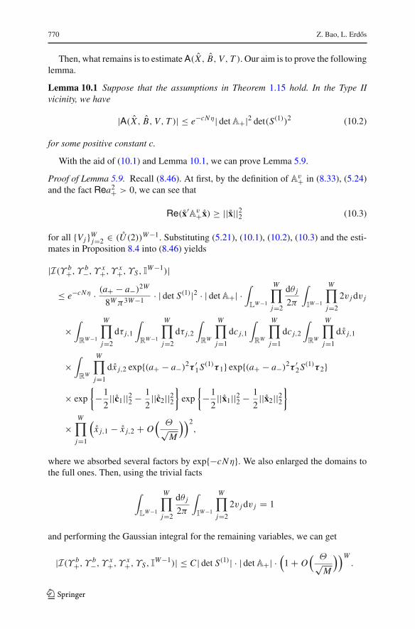
770 Z. Bao, L. Erdos
Then, what remains is to estimateA(X , B, V, T ). Our aim is to prove the followinglemma.
Lemma 10.1 Suppose that the assumptions in Theorem 1.15 hold. In the Type IIvicinity, we have
|A(X , B, V, T )| ≤ e−cNη| detA+|2 det(S(1))2 (10.2)
for some positive constant c.
With the aid of (10.1) and Lemma 10.1, we can prove Lemma 5.9.
Proof of Lemma 5.9. Recall (8.46). At first, by the definition of Av+ in (8.33), (5.24)and the fact Rea2+ > 0, we can see that
Re(x′Av+x) ≥ ||x||22 (10.3)
for all {Vj }Wj=2 ∈ (U (2))W−1. Substituting (5.21), (10.1), (10.2), (10.3) and the esti-mates in Proposition 8.4 into (8.46) yields
|I(Υ b+, Υ b−, Υ x+, Υ x+, ΥS, IW−1)|
≤ e−cNη · (a+ − a−)2W
8Wπ3W−1 · | det S(1)|2 · | detA+| ·∫
LW−1
W∏
j=2
dθ j2π
∫
IW−1
W∏
j=2
2v jdv j
×∫
RW−1
W∏
j=2
dτ j,1
∫
RW−1
W∏
j=2
dτ j,2
∫
RW
W∏
j=1
dc j,1
∫
RW
W∏
j=1
dc j,2
∫
RW
W∏
j=1
dx j,1
×∫
RW
W∏
j=1
dx j,2 exp{(a+ − a−)2τ ′1S(1)τ 1} exp{(a+ − a−)2τ ′
2S(1)τ 2}
× exp
{
−1
2||c1||22 − 1
2||c2||22
}
exp
{
−1
2||x1||22 − 1
2||x2||22
}
×W∏
j=1
(
x j,1 − x j,2 + O( Θ√
M
))2,
where we absorbed several factors by exp{−cNη}. We also enlarged the domains tothe full ones. Then, using the trivial facts
∫
LW−1
W∏
j=2
dθ j2π
∫
IW−1
W∏
j=2
2v jdv j = 1
and performing the Gaussian integral for the remaining variables, we can get
|I(Υ b+, Υ b−, Υ x+, Υ x+, ΥS, IW−1)| ≤ C | det S(1)| · | detA+| ·
(
1 + O( Θ√
M
))W.
123

Delocalization for a class of random block band matrices 771
(10.4)
Observe that
| detA+| ≤ |1 + a2+|W ≤ 2W . (10.5)
Moreover, by Assumption 1.1 (ii), we see that |si i | ≤ (1 − c0)/2 for some smallpositive constant c0. Consequently, since S(1) is negative definite, we have
| det S(1)| ≤∏
i �=1
|si i | ≤(1 − c0
2
)W(10.6)
by Hadamard’s inequality. Substituting (10.5) and (10.6) into (10.4) yields
|I(Υ b+, Υ b−, Υ x+, Υ x+, ΥS, IW−1)| = O(e−cW ) (10.7)
for some positive constant δ. Hence, we proved the first part of Lemma 5.9. The secondpart can be proved analogously. ��
In the sequel, we prove Lemma 10.1. We also ignore the factor Q(·) from thediscussion at first.
10.1 P(X, B, V, T ) in the Type II vicinity
Lemma 10.2 Suppose that the assumptions in Theorem 1.15 hold. In the Type IIvicinity, we have
|P(X , B, V, T )| ≤ W 2+γΘ2
M| detA+|2 det(S(1))2. (10.8)
Proof We will follow the strategy in Sect. 9.1. We regard all V -variables as fixedparameters. Now, we define the function
ι ≡ ι j (X , B, T ) := |x j,1| + |x j,2| + |b j,1| + |b j,2| + |t j |.
Then, we recall the representation (9.4) and the definition of Δ�, j in (9.5). We stilladopt the representation (9.8). It is easy to see that in the Type II vicinity, we also havethe bound (9.9) for p�, j,α,β . The main difference is the first factor of the r.h.s. of (9.4).We expand it around the saddle point as
exp{
− TrV ∗j X
−1j V jΩ j T
−1j B−1
j TjΞ j
}
=: exp{
− TrD−1+ Ω j D−1± Ξ j
}
× exp{
− 1√MΔ j
}
.
123

772 Z. Bao, L. Erdos
We take the formula above as the definition of Δ j , which is of the form
Δ j =4∑
α,β=1
p j,α,β · ω j,αξ j,β ,
where p j,α,β is a function of X , B, V and T -variables, satisfying
p j,α,β = O(ι).
Let H = (a−2+ A+) ⊕ S ⊕ (a−2+ A+) ⊕ S. Recalling the notation in (6.16), we canwrite
−∑
j,k
s jkT rΩ jΞk −W∑
j=1
TrD−1+ Ω j D−1± Ξ j = −�H�′.
Now, via replacingΔ1, j by Δ1, j , κ j by ι j ,H by H in the proof of Lemma 9.2, we canperform the proof of Lemma 10.2 in the same way. We leave the details to the reader.
��
10.2 F(X, B, V, T ) in the Type II vicinity
Lemma 10.3 Suppose that the assumptions in Theorem 1.15 hold. In the Type IIvicinity, we have
F(X , B, V, T ) = O
(
exp{−(a+ − a−)Nη}(Nη)n+1
)
. (10.9)
Proof Recall the decomposition (9.34). Note that Lemma9.9 is still applicable.Hence,it suffices to estimate F(X , V ). Now, note that in the Type II vicinity, it is easy to seethat
W∑
j=1
Tr X j J = O( ||x1||1 + ||x2||1√
M
)
= O( Θ√
M
))
.
Consequently, by the assumption on η, we have
exp
⎧
⎨
⎩
MηW∑
j=1
Tr X j J
⎫
⎬
⎭
= exp{O(Θ√Mη)} = 1 + o(1).
From (3.20) we can also see that all the other factors of f (P1, V, X , X [1]) are O(1).Hence, by the definition (9.33), we have F(X , V ) = O(exp{−(a+ − a−)Nη}), whichtogether with Lemma 9.9 yields the conclusion. ��
123

Delocalization for a class of random block band matrices 773
10.3 Summing up: Proof of Lemma 10.1
Analogously, we shall slightly modify the proofs of Lemma 10.2 and Lemma 10.3, inorder to take Q(·) into account. The proof can then be performed in the same manneras Lemma 9.1. We omit the details.
11 Proof of Theorem 1.15
The conclusion for Case 1 is a direct consequence of the discussions in Sects. 3.5–10.More precisely, by using Lemmas 5.1, 5.6, 5.8 and 5.9, we can get (1.21) immediately.
The proofs of Case 2 and Case 3 can be performed analogously, with slight modifi-cations, which will be stated below. In Case 2, we shall slightly modify the discussionsin Sects. 3.5–10 for Case 1, according to the decomposition of supermatrices in (3.9).Now, at first, in (3.12) and (3.13), for A = S, X , Y , Ω or Ξ , we replace A〈1〉
p and A〈1〉q
by A〈1,2〉p and Aq respectively, and replace A[1]
q by A[2]p . In addition, in the last three
lines of (3.13), we shall also replace s jq by s j p, and replace s pq and sqp by s pp, andin the first line, we replace φ1,q,1φ1,p,1φ2,p,1φ2,q,1 by φ1,p,2φ1,p,1φ2,p,1φ2,p,2. Then,
in (3.14) and (3.15), for A = X,Y,Ω,Ξ,ω, ξ ,w, y, u, v or σ , we replace A[1]q by
A[2]p . With these modifications, it is easy to check the proof in Sects. 3.5–10 applies to
Case 2 as well. The main point is we can still gain the factor 1/(Nη)n+1 from integralof g(·) defined in (3.21) (with y[1]
q and w[1]q replaced by y[2]
p and w[2]p ). Heuristically,
we can go back to (4.4), and replace σ [1]q by σ [2]
p therein. It is then quite clear thesame estimate holds. Consequently, Lemmas 5.1, 5.6, 5.8 and 5.9 still hold under thereplacement of the variables described above. Hence, (1.21) holds in Case 2.
In Case 3, we can also mimic the discussions for Case 1 with slight modifica-tions. We also start from (3.12) and (3.13). For A = S, X , Y , Ω, Ξ ,ω and ξ , wereplace A〈1〉
q by Aq , and replace A[1]q by 0. In addition, in the first line of (3.13), we
replace φ1,q,1φ1,p,1φ2,p,1φ2,q,1 by φ1,p,1φ1,p,1φ2,p,1φ2,p,1. Consequently, after using
superbosonization formula, we will get the factor (y[1]p |(w[1]
p (w[1]p )
∗)12|)2n instead of
(y[1]p y[1]
q (w[1]q (w
[1]q )
∗)12(w[1]p (w
[1]p )
∗)21)n in (3.16). Then, for the superdeterminantterms
∏
k=p,q
det(Xk −Ωk(Yk)−1Ξk)
det Yk,
∏
k=p,q
y[1]k
(
y[1]k − ξ
[1]k (X
[1]k )
−1ω[1]k
)2
det2(X [1]k )
.
we shall only keep the factors with k = p and delete those with k = q. Moreover,we shall also replace A[1]
q by 0 for A = X,Y,Ω,Ξ,ω, ξ ,w, y, u, v or σ in (3.16).
In addition, dA[1] shall be redefined as the differential of A[1]p -variables only, for
A = X, y,w,w and ξ . One can check step by step that such a modification does notrequire any essential change of our discussions for Case 1. Especially, note that ourmodification has nothing to do with the saddle point analysis on the Gaussian measureexp{−M(K (X , V )+ L(B, T ))}. Moreover, the term P(·) in (3.29) can be redefinedby deleting the factor with k = q in the last term therein. Such a modification does not
123

774 Z. Bao, L. Erdos
change our analysis of P(·). In addition, the irrelevant term Q(·) can also be definedaccordingly. Specifically, we shall delete the factor with k = q in the last term of(3.30) and replace A[1]
q by 0 for A = Ω,Ξ,ω, ξ ,w, y. It is routine to check thatLemma 6.3 still holds under such a modification. Analogously, we can redefine thefunctionsF(·), f (·) and g(·) in (3.19)–(3.21). Now, the main difference between Case3 and Case 1 or 2 is that the factor (y[1]
p |(w[1]p (w
[1]p )
∗)12|)2n does not produce oscilla-tion in the integral of g(·) any more. Heuristically, the counterpart of (4.4) in Case 3reads
e(a+−a−)Nη∫
dy[1]dw[1]dν(Q1) · g(B, T, Q1, y[1],w[1])
∼∫ ∞
02tdt
∫
L
dσ [1]p · e−cNηt2+c1e
−iσ [1]p t ∼ 1
Nη.
Hence, (1.21) holds for Case 3. Therefore, we completed the proof of Theorem 1.15.
12 Comment on the prefactor NC0 in (1.21)
In the proof of (1.21), we have used NC0 to replace MΘ2WC0/(Nη)� (see the proofof Lemma 5.8). However, the latter is also artificial. It can be improved to somen-dependent constant Cn via a more delicate analysis on A(·), i.e. the integral ofP(·)Q(·)F(·). Such an improvement stems from the cancellation in the Gaussianintegral. At first, a finer analysis will show that the factor Q(·) can really be ignored,in the sense that it does not play any role in the estimate of the order of E|Gi j (z)|2n .Hence, for simplicity, we just focus on the product P(·)F(·) instead of A(·). Then,we go back to Lemmas 9.2 and 9.7. Recall the decomposition (9.34). A more carefulanalysis on F(·) leads us to the following expansion, up to the subleading order termsof the factors G(·) and F(·),
F(·) = G(·)F(·) ∼ 1
(Nη)n+2
⎛
⎝1 + Mη√M
W∑
j=1
l j (x j,1, x j,2, v j )+ · · ·⎞
⎠
×⎛
⎝1 + Mη√M
W∑
j=1
l′j (b j,1, b j,2, t j )+ · · ·⎞
⎠ , (12.1)
where l j (·)’s and l′j (·)’s are some linear combinations of the arguments. Analogously,
we shall write down the leading order term of P(·) in terms of x, b, t and v explicitly.Then it can be seen that the leading order term of P(·) is a linear combination ofx j,1 xk,2, b j,1bk,2, x j,α bk,β , υ j,ατk,β for j, k = 1, . . . ,W and α, β = 1, 2, in whichall the coefficients are of order 1/M . Observe that the Gaussian integral in (8.45) willkill the linear terms. Consequently, in the expansion (12.1), the first term that survives
123
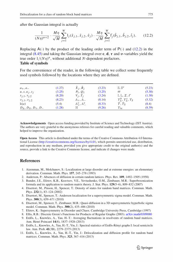
Delocalization for a class of random block band matrices 775
after the Gaussian integral is actually
1
(Nη)n+2 · Mη√M
W∑
j=1
l j (x j,1, x j,2, v j ) · Mη√M
W∑
j=1
l′j (b j,1, b j,2, t j ). (12.2)
Replacing A(·) by the product of the leading order term of P(·) and (12.2) in theintegral (8.45) and taking the Gaussian integral over c,d, τ and υ-variables yield thetrue order 1/(Nη)n , without additional N -dependent prefactors.Table of symbols
For the convenience of the reader, in the following table we collect some frequentlyused symbols followed by the locations where they are defined.
a+, a− (1.27) X j , B j (3.23) S, Sv (5.23)u, s, u j , s j (3.25) P1, Q1 (3.25) Θ (5.30)τ j,1, τ j,2 (8.20) Vj , Tj (3.24) I,L,Σ, Γ (1.30)υ j,1, υ j,2 (8.23) A+,A− (8.14) Υ b±, Υ x±, ΥS (5.32)k(a) (5.4) A
v+,Av− (8.33) Υ , ΥS (8.4)D±, D∓, D+, D− (1.28) H (9.26) Υ∞ (8.39)
Acknowledgements Open access funding provided by Institute of Science and Technology (IST Austria).The authors are very grateful to the anonymous referees for careful reading and valuable comments, whichhelped to improve the organization.
Open Access This article is distributed under the terms of the Creative Commons Attribution 4.0 Interna-tional License (http://creativecommons.org/licenses/by/4.0/), which permits unrestricted use, distribution,and reproduction in any medium, provided you give appropriate credit to the original author(s) and thesource, provide a link to the Creative Commons license, and indicate if changes were made.
References
1. Aizenman, M., Molchanov, S.: Localization at large disorder and at extreme energies: an elementaryderivation. Commun. Math. Phys. 157, 245–278 (1993)
2. Anderson, P.: Absences of diffusion in certain random lattices. Phys. Rev. 109, 1492–1505 (1958)3. Bunder, J.E., Efetov, K.B., Kravtsov, V.E., Yevtushenko, O.M., Zirnbauer, M.R.: Superbosonization
formula and its application to random matrix theory. J. Stat. Phys. 129(5–6), 809–832 (2007)4. Disertori, M., Pinson, H., Spencer, T.: Density of states for random band matrices. Commun. Math.
Phys. 232(1), 83–124 (2002)5. Disertori, M., Spencer, T.: Anderson localization for a supersymmetric sigma model. Commun. Math.
Phys. 300(3), 659–671 (2010)6. Disertori, M., Spencer, T., Zirnbauer, M.R.: Quasi-diffusion in a 3D supersymmetric hyperbolic sigma
model. Commun. Math. Phys. 300(2), 435–486 (2010)7. Efetov, K.: Supersymmetry in Disorder and Chaos. Cambridge University Press, Cambridge (1997)8. Ellis, R.B.: Discrete Green’s Functions for Products of Regular Graphs (2003). arXiv:math/03090809. Erdos, L., Knowles, A., Yau, H.-T.: Averaging fluctuations in resolvents of random band matrices.
Ann. Henri Poincaré 14(8), 1837–1926 (2013)10. Erdos, L., Knowles, A., Yau, H.-T., Yin, J.: Spectral statistics of Erdos-Rényi graphs I: local semicircle
law. Ann. Prob. 41(3B), 2279–2375 (2013)11. Erdos, L., Knowles, A., Yau, H.-T., Yin, J.: Delocalization and diffusion profile for random band
matrices. Commun. Math. Phys. 323, 367–416 (2013)
123

776 Z. Bao, L. Erdos
12. Erdos, L., Knowles, A., Yau, H.-T., Yin, J.: The local semicircle law for a general class of randommatrices. Electron. J. Probab 18(59), 1–58 (2013)
13. Erdos, L., Schlein, B., Yau, H.-T.: Local semicircle law and complete delocalization forWigner randommatrices. Commun. Math. Phys. 287, 641–655 (2009)
14. Erdos, L., Yau, H.-T., Yin, J.: Bulk universality for generalizedWigner matrices. Probab. Theory Relat.Fields 154(1–2), 341–407 (2012)
15. Fröhlich, J., Spencer, T.: Absence of diffusion in the Anderson tight binding model for large disorderor low energy. Commun. Math. Phys. 88, 151–184 (1983)
16. Fyodorov, Y.V., Mirlin, A.D.: Scaling properties of localization in random band matrices: a σ -modelapproach. Phys. Rev. Lett. 67, 2405–2409 (1991)
17. Klein, A.: Extended states in the Anderson model on the Bethe lattice. Adv. Math. 133(1), 163–184(1998)
18. Littelmann, P., Sommers, H.J., Zirnbauer, M.R.: Superbosonization of invariant randommatrix ensem-bles. Commun. Math. Phys. 283(2), 343–395 (2008)
19. Shcherbina, T.: On the second mixed moment of the characteristic polynomials of 1D band matrices.Commun. Math. Phys. 328(1), 45–82 (2014)
20. Shcherbina, T.: Universality of the local regime for the block band matrices with a finite number ofblocks. J. Stat. Phys. 155(3), 466–499 (2014)
21. Shcherbina, T.: Universality of the second mixed moment of the characteristic polynomials of the 1Dband matrices: real symmetric case (2014). arXiv:1410.3084
22. Schäfer, L., Wegner, F.: Disordered system with n orbitals per site: Lagrange formulation, hyperbolicsymmetry, and Goldstone modes. Z. Phys. B 38, 113–126 (1980)
23. Schenker, J.: Eigenvector localization for random bandmatrices with power law band width. Commun.Math. Phys. 290, 1065–1097 (2009)
24. Sodin, S.: An estimate for the average spectral measure of random band matrices. J. Stat. Phys. 144(1),46–59 (2011)
25. Sodin, S.: The spectral edge of some random band matrices. Ann. Math. 172(3), 2223–2251 (2010)26. Spencer, T.: SUSY Statistical Mechanics and Random Band Matrices, QuantumMany Body Systems.
Springer, Berlin Heidelberg (2012)27. Spencer, T., Zirnbauer, M.R.: Spontaneous symmetry breaking of a hyperbolic sigma model in three
dimensions. Commun. Math. Phys. 252(1–3), 167–187 (2004)28. Tao, T., Vu, V.: Random matrices: universality of local eigenvalue statistics. Acta Math. 206(1), 127–
204 (2011)29. Wang, W.M.: Mean field upper and lower bounds on Lyapunov exponents. Am. J. Math. 851-878
(2002)30. Wegner, F.J.: Disordered system with n orbitals per site: n → ∞ limit. Phys. Rev. B 19, 783–792
(1979)31. Wigner, E.: Characteristic vectors of bordered matrices with infinite dimensions. Ann. Math. 62, 548–
564 (1955)
123