Quantitative Strategies Research Notesjanroman.dhis.org/finance/Numerical Methods/enhanced_numerical_… · gest a method for enhancing the numerical solution ... See Derman and Kani

Quantitative StrategiesResearch Notes

GoldmanSachs

Enhanced Numerical Methodsfor Options with Barriers

Emanuel DermanIraj KaniDeniz ErgenerIndrajit Bardhan

May 1995

QUANTITATIVE STRATEGIES RESEARCH NOTESSachsGoldman

Copyright 1995 Goldman, Sachs & Co. All rights reserved.

This material is for your private information, and we are not soliciting any action based upon it. This report is not tobe construed as an offer to sell or the solicitation of an offer to buy any security in any jurisdiction where such an offeror solicitation would be illegal. Certain transactions, including those involving futures, options and high yieldsecurities, give rise to substantial risk and are not suitable for all investors. Opinions expressed are our presentopinions only. The material is based upon information that we consider reliable, but we do not represent that it isaccurate or complete, and it should not be relied upon as such. We, our affiliates, or persons involved in thepreparation or issuance of this material, may from time to time have long or short positions and buy or sell securities,futures or options identical with or related to those mentioned herein.

This material has been issued by Goldman, Sachs & Co. and/or one of its affiliates and has been approved byGoldman Sachs International, regulated by The Securities and Futures Authority, in connection with its distributionin the United Kingdom and by Goldman Sachs Canada in connection with its distribution in Canada. This material isdistributed in Hong Kong by Goldman Sachs (Asia) L.L.C., and in Japan by Goldman Sachs (Japan) Ltd. Thismaterial is not for distribution to private customers, as defined by the rules of The Securities and Futures Authorityin the United Kingdom, and any investments including any convertible bonds or derivatives mentioned in thismaterial will not be made available by us to any such private customer. Neither Goldman, Sachs & Co. nor itsrepresentative in Seoul, Korea is licensed to engage in securities business in the Republic of Korea. Goldman SachsInternational or its affiliates may have acted upon or used this research prior to or immediately following itspublication. Foreign currency denominated securities are subject to fluctuations in exchange rates that could have anadverse effect on the value or price of or income derived from the investment. Further information on any of thesecurities mentioned in this material may be obtained upon request and for this purpose persons in Italy shouldcontact Goldman Sachs S.I.M. S.p.A. in Milan, or at its London branch office at 133 Fleet Street, and persons in HongKong should contact Goldman Sachs Asia L.L.C. at 3 Garden Road. Unless governing law permits otherwise, youmust contact a Goldman Sachs entity in your home jurisdiction if you want to use our services in effecting atransaction in the securities mentioned in this material.

Note: Options are not suitable for all investors. Please ensure that you have read and understood thecurrent options disclosure document before entering into any options transactions.

-1


SUMMARY

Most real-world barrier options have no analyticsolutions, either because the barrier structure iscomplex or because of volatility skews in the market.Numerical solutions are a necessity. But optionswith barriers are notoriously difficult to valuenumerically on binomial or multinomial trees, or onfinite-difference lattices. Their values converge veryslowly as the number of tree or lattice levelsincrease, often requiring unattainably large comput-ing times for even a modest accuracy.

In this paper we analyze the biases implicit in valu-ing options with barriers on a lattice. We then sug-gest a method for enhancing the numerical solutionof boundary value problems on a lattice that helps tocorrect these biases. It seems to work well in prac-tice.

_______________________________

New York:

Emanuel Derman (212) 902-0129Iraj Kani (212) 902-3561Deniz Ergener (212) 902-4673

London:

Indrajit Bardhan (171) 774-1666

________________________________

We thank Barbara Dunn for comments on the manu-script.

1


As derivative markets have matured, options with barriers1 have becomeincreasingly popular because of the greater precision with which theyallow investors to obtain or avoid exposure. The value of a knockin stock(or index) option depends sensitively on the risk-neutral probability of thestock being in-the-money and beyond the barrier. Similarly, the value of aknockout option depends on the probability of the stock being in-the-money but not beyond the barrier. The analytic solution for these probabil-ities, and for the value of a European-style knockout option on stock underthe standard Black-Scholes assumptions, was published by Merton (1973).This analytic solution provides rapidly computed, accurate values andhedge ratios, so important for managing the risk of large books of exoticand standard options.

Many of the currently traded barrier-style derivatives have no analyticsolutions. The analytic method works only for simple barriers at a fixed orexponentially rising level, assuming lognormal stock price evolution andEuropean-style exercise. There are now over-the-counter markets inoptions whose barriers may have arbitrary time dependence, whoseimplied volatilities exhibit a skew that corresponds to non-lognormal evo-lution of the underlying stock price2, or whose exercise may be American-style. In most of these cases there exists no general analytic solution forthe value of the barrier option, and so a numerical solution is unavoidable.The most common numerical techniques involve solving the differentialequation on a binomial lattice (Cox, Ross and Rubinstein 1979), usingmore general (explicit or implicit) finite difference methods, or using theMonte Carlo method of integral evaluation (Boyle 1977). The numericalaccuracy of these methods becomes an important issue.

The binomial method for standard European-style options convergesfairly rapidly as the number of levels on the binomial tree increases. Fig-ure 1 shows the variation in value with level number for a typical case.You can see that the answer is accurate to better than 0.4% for binomialtrees of greater than 40 levels; the values oscillate about the analyticvalue of 12.99 as you increment the number of levels, and approach thecorrect analytic value asymptotically.

In contrast, the binomial method for barrier options converges very slowlyas the number of binomial levels increases, especially when the barrier isclose to spot, as first pointed out by Margrabe (1989). Figure 2 illustratesthe convergence of the binomial value of a representative down-and-out

1. For an overview of barrier options and their uses, see, for example, Derman and Kani(1993).2. See Derman and Kani (1994), Rubinstein (1994), Dupire (1994).

THE PROBLEM WITHBARRIER OPTIONS

2


call option to its analytic value. The solution approaches the analyticvalue of 7.31 in a sawtooth fashion, with severe periodic spikes thatmove away from the correct result. The magnitude of the spikesattenuate so slowly with increasing periods that even between 900and 1100 periods, as shown in the inset to Figure 2, the amplitude ofthe error due to the spike is 0.60, or about 8.2% of the correct theoret-ical option value. It may take tens of thousands of periods before thevalue converges to within 1%. Trinomial trees, implicit, explicit andother finite-difference methods suffer from similar problems.

In this paper we analyze the cause of this unsatisfactory conver-gence, and explain and illustrate a general method for improving it.Our method is applicable to all types of finite-difference methods.

FIGURE 1. Convergence to analytic value of a binomially-valued one-year European call option as the number of binomial levels increases.We assume an index level of 100, a strike of 100, an annuallycompounded riskless interest rate of 10% per year, zero dividendyield, and a volatility of 20%. The analytic value is 12.99.

Option Value

binomial

analytic

levels

10

20

30

40

50

60

70

80

90

10

01

10

12

01

30

14

01

50

16

01

70

18

01

90

20

0

12.75

12.85

12.95

13.05

13.15

13.25

12.99

3


Option Value

binomial

analytic

levels

10

20

30

40

50

60

70

80

90

10

01

10

12

01

30

14

01

50

16

01

70

18

01

90

20

0

7.00

8.00

9.00

10.00

11.00

FIGURE 2. Convergence to analytic value of a binomially-valued one-year European down-and-out call option as the number of binomiallevels increases. We assume an index level of 100, a strike of 100, abarrier level of 95, an annually compounded riskless interest rate of10% per year, zero dividend yield, and a volatility of 20%. The analyticvalue is 7.31. Inset shows convergence between 900 and 1100 binomiallevels.

7.31

90

0 9

50

10

00

10

50

11

00

7.20

7.95

4


Options valuation often involves the solution of a boundary-valueproblem. You know the future payoffs of the option at its terminalboundaries, as dictated by the contract. The ability to hedge with theunderlier dictates the replication strategy (and the correspondingcontinuous-time differential equation) that relates these future pay-offs to the present fair value. To solve the differential equationnumerically, you convert it to a finite difference equation on a dis-crete underlier value- and time-lattice, and then solve this equation.As you decrease the size of the lattice spacing, you get closer to thecontinuous-time result3.

There are (at least) two sources of inaccuracy in modeling options ona lattice. In most of this paper we will illustrate our methods throughthe use of the generally familiar binomial tree for stock prices, but westress that the same effects appear in any lattice scheme.

The first type of inaccuracy is caused by the unavoidable existence ofthe lattice itself, which “quantizes” the stock price and the instants intime at which it can be observed. Figure 3 contains a binomial latticefor a stock that moves up or down by $10 every year. We choose thesecoarse arithmetic (rather than geometric) increments to the stockprice so as to keep the illustration simple rather than realistic. Onceyou’ve chosen a lattice, the stock is allowed to take the values of onlythose points on the lattice. In essence, when you use a lattice you arevaluing an option on a stock that moves discretely. We call this unre-alistic lack of continuity quantization error. It leads to an option pricethat is theoretically correct only for a stock that actually displayssuch quantized behavior; if you want to use the model for options onreal stocks that move almost continuously, you must use a latticewith an infinitesimal mesh, or at least one small enough so that fur-ther reduction in its spacing has negligible numerical effect.

The second type of inaccuracy occurs because of the inability of thelattice to accurately represent the terms of the option. Once you’vechosen a lattice, the available stock prices are fixed. If the exerciseprice or barrier level of the option doesn’t coincide with one of theavailable stock prices, you effectively have to move the exercise price

3. Real stocks trade at discrete times, with discrete ticks, pay discrete dividends,and trade only during certain periods. In some contracts barriers are only operativeat certain times of day. In the interests of precise modeling, you may sometimes notwant to proceed all the way to the continuous-time limit, but rather preserve the con-tract’s or market’s discreteness. We ignore these effects here, and assume that stockprices can move continuously.

ERRORS ON A LATTICE

Stock PriceQuantization Error

OptionSpecification Error

5


or barrier to the closest stock price available. Then, the option youvalue on the lattice has contractual terms that differ from those ofthe actual option. We call this specification error.

We will show that for barrier options, specification error vanishesmuch more slowly than quantization error. However, you can adjustlattice methods for specification error to get a much improved result.

Consider a standard at-the-money call, struck at 100, with five yearsto expiration. Even on a coarse stock lattice you can choose a mesh sothat a set of stock nodes coincide with the expiration time of fiveyears. In Figure 4 we show the payoff of this call at the heavy expira-tion boundary on the binomial lattice of Figure 3. At all availablenodes at expiration where the call’s payoff is defined by the contract,the option’s payoff is strictly correct. There is no specification error,only quantization error: only the movement of the stock is being mod-

100

110

90

120

100

80

130

110

90

140

120

100

80

60

150

130

110

90

70

50

70

year 0 1 2 3 4 5

FIGURE 3. A sample binomial stock lattice. The stock price (rather thanits return) undergoes a simple arithmetic Brownian motion with avolatility of 10 points once a year. Although this is unrealistic, itmakes the numerical examples simpler to explain, without giving upanything essential.

Standard Optionson a Lattice:Quantization Error

6


eled unrealistically. As long as the final nodes of the tree are placedat times corresponding to the expiration of the option, you are alwaysvaluing the correct option. As the number of binomial levels isincreased, the quantization error diminishes. This behavior is mani-fested in Figure 1, where, in addition, because successive tree levelsalternate between even and odd numbers of nodes, the quantizationerror about the analytic solution alternates in sign.

Let’s look at an up-and-out European-style call option struck at 70,with five years to expiration and a knockout barrier at 120. Figure 5shows the boundary values of this call on the sample binomial latticeof Figure 3. There are a set of tree nodes that lie exactly on the expi-ration boundary, so the payoff at each node is exactly the value dic-tated by the terms of the call contract. There are also a set of nodesthat lie exactly on the knockout boundary at 120, so the payoff ateach node on the knockout boundary is also correct. There is no spec-ification error on the lattice; the only inaccuracy in the valuation of

FIGURE 4. The payoff of a five-year call struck at 100 on the binomiallattice of Figure 3. Call prices on the heavy expiration boundary areshown in bold type.

100

110

90

120

100

80

130

110

90

140

120

100

80

60

150

130

110

90

70

50

70

50

30

10

0

0

0

strike

year 0 1 2 3 4 5

Barrier Optionson a Lattice:Quantization andSpecification Error

7


the call occurs from quantization error — the lattice mesh is toocoarse to represent realistic stock price behavior. In the limit as thelattice mesh becomes infinitesimally small, the errors will vanish.

In contrast, Figure 6 shows a similar call with a knockout barrier at125. Because the barrier falls between the nodes at 120 and 130, thelattice first “feels” the effect of the barrier at 130, in the sense thatthe nodes at 130 are the lowest-price nodes where the knockoutboundary condition can be logically applied. So, call values at thenodes at 130 are set to zero. We call 130 the effective barrier.

If you now use this lattice to value the option, there are two ways inwhich you are valuing the wrong option. First, you are valuing anoption whose barrier is really at 130 instead of 125. Second, as wasthe case with the standard option, the stock evolution is unrealisti-cally coarse. As you decrease the lattice spacing, the effective barrier

FIGURE 5. The payoff of a five-year up-and-out call struck at 70 withknockout barrier at 120, illustrated on the binomial lattice of Figure 3.The specified expiration boundary and the barrier are denoted by aheavy line. Call payoffs on these boundaries are shown in bold type.

100

110

90

120

100

80

130

110

90

140

120

100

80

60

150

130

110

90

70

50

70

year 0 1 2 3 4 5

40

20

0

0

00

specified

barrier B

8


moves closer to the specified barrier — the specification error dimin-ishes — and the stock evolution becomes more nearly continuous.From the point of view of accuracy, this situation is worse than theone for standard options, where the specification error was zero forany lattice spacing, and only the stock evolution was discontinuous.This is the reason for the worse convergence in Figure 2 comparedwith Figure 1.

FIGURE 6. The payoff of a five-year up-and-out call struck at 70 withknockout barrier at 125, illustrated on the binomial lattice of Figure 3.The specified barrier lies at 125. The effective barrier at which thelattice first perceives the effect of the knockout lies at 130.

100

110

90

120

100

80

130

110

90

140

120

100

80

60

150

130

110

90

70

50

70

year 0 1 2 3 4 5

40

20

0

0

00

specified barrier B

effective barrier E

0

9


Boyle and Lau (1994) have recently pointed out a method of improv-ing binomial lattice valuation in certain cases. If you look at the saw-tooth pattern of convergence in Figure 2, you can see that forbinomial trees with about 15, 60 or 138 levels, the binomial value isvery close to the correct analytical value. The reason is that for thesenumbers of levels, the barrier falls almost exactly on the nodes and,in our language, the specification error is close to zero.

For a Cox-Ross-Rubinstein (1979) tree (a CRR tree) with N periods to

expiration, a barrier at stock level B lies exactly m nodes away from

the current stock price S when or

(EQ 1)

This argument relies on the fact that the locations of the stock nodesof a CRR tree are independent of the riskless interest rate, and lie atthe same stock levels at all times.

If the barrier level varies with time, or a different (non-CRR) tree isused, you cannot easily force the specification error to be zero byusing Boyle and Lau’s procedure. Therefore, we seek a method thatcorrects for the specification error no matter what the shape of thelattice or where the barrier falls relative to the lattice.

We’ll illustrate our strategy by referring to the option in Figure 6, inwhich the effective barrier lies at 130 but the (true) specified barrierlies at 125. When you value the option on this tree, the computedoption values at the first set of tree nodes just inside the specifiedbarrier will be incorrect, because they have been naively computedfrom a knockout at the effective barrier rather than at the specifiedbarrier. We call this first set of nodes with computed values the modi-fied barrier, and display it in Figure 4. The values on these modifiedbarrier nodes obtained by valuing the option using backward induc-tion from the effective barrier are larger than they should be, becausethe contract dictates that the call knocks out at 125, and the binomiallattice first “feels” the knockout at 130.

Therefore, in the interests of accuracy, we must adjust the naively-computed values at the modified barrier nodes. We will replace themby values that more accurately reflect their closer proximity to theknockout barrier at the specified level of 125. After modifying the val-

ELIMINATINGSPECIFICATION ERRORFOR BARRIER OPTIONS

S mσ TN-----

exp B=

N m2σ2T( ) lnBS----⁄= m 1 2 ....,±,±=

The Modified BarrierMethod

10


ues at the modified barrier, we will continue with valuation by back-ward induction towards the root of the tree, and so obtain the currentoption value.

What’s the right way to modify the naively-computed values on themodified barrier? First, notice that the naive values at all tree nodesare appropriate for an option contract with barrier level at the effec-tive barrier E. Their only inaccuracy is due to quantization error.Therefore, you can use this naive tree with knockout occurring at theeffective barrier to compute a reasonably accurate finite-difference

approximation for the . This is the rate at which the

barrier option’s value C varies with stock price S near its effectivebarrier E at all future times t. This derivative is also a good approxi-mation for the rate at which the value of the option, with knockoutoccurring at the specified barrier B, grows away from the barrier.

FIGURE 7. The modified barrier for the knockout option of Figure 6.Stock prices are shown in plain type. Call payoffs are shown in bold.

100

110

90

120

100

80

130

110

90

140

120

100

80

60

150

130

110

90

70

50

70

year 0 1 2 3 4 5

40

20

0

0

0

0specified barrier B

effective barrier E

modified barrier

0

S∂∂C S E t, ,( )

S E=

11


Because the distance between the specified barrier B and the effec-tive barrier E is small, the rate at which a barrier option value growsaway from the barrier is independent of the location of the barrier tofirst order, that is

(EQ 2)

Equation 2 provides an estimate for the derivative, at the barrier B,of the value of the option with knockout occurring at barrier B. Wecan use this derivative to develop a first-order Taylor expansion forthe option value about its specified barrier, and so get a more accu-rate value of the option on its modified barrier. We can then value theoption by backward recursion from this modified barrier to find amore accurate solution.

That’s the procedure for enhancing the value of a knockout option. Ifthe option C knocks into a target option T on a barrier B that liesbetween tree levels, we can use the same reasoning to obtain the esti-mated value of T on the specified barrier. Use the naive tree with the

effective barrier to get an estimate for . Then use

this derivative to develop a first-order Taylor expansion that com-putes the value of T(B) on the specified barrier from its zeroth-ordervalue on the modified barrier. This value of T(B) provides anenhanced estimate for the value of the target option on the specifiedbarrier. This value is then used as the zeroth-order term in a first-order Taylor expansion for the value of the barrier option on the mod-ified barrier. The method is illustrated in detail in A BINOMIAL EXAMPLE

on page 17.

To summarize, the modified barrier method is a sort of bootstrapmethod. You first value the (slightly) wrong option by backwardinduction from the wrong (effective) barrier to get (almost) rightnumerical values for the derivative of the true option at all times onits barrier. You then use these derivatives at each level of the tree ina first-order Taylor series on the barrier to obtain modified barriervalues for the true option. Finally, you value the correct option bybackward induction from the modified barrier.

S∂∂C S E t, ,( )

S E= S∂∂C S B t, ,( )

S B=O B E–( )2( )+=

S∂∂T S E t, ,( )

S E=

12


Consider an option with value V(S) that knocks into a target securityT(S) if the stock price S crosses a barrier B. (You can think of T(S) asbeing zero for a knockout option that pays no rebate.) Figure 8 showsthe method we use to correct the values on the modified barrier.

1. Value the target option T(S) and the barrier option V(S) at eachnode on the tree with the barrier at the effective barrier.

The Modified BarrierAlgorithm

FIGURE 8. The modified barrier algorithm on a binomial tree. U is theup-node on the effective barrier above the specified barrier.B represents the specified barrier that in general falls between an up-and a down-node. D is the down-node on the modified barrier belowthe specified barrier. V(S) is the value of the barrier option at stockprice S, assuming the specified barrier coincides with the effectivebarrier. T(S) is the value of the target option which V(S) knocks into onthe effective barrier. is the adjusted value of the barrier optionon the modified barrier.

V D( )

specified barrier

U

D

effective barrier

B

modified barrier

T B( ) T D( ) ∆T B D–( )+=

V U( ) T U( ),

V D( ) T D( ),

Taylorexpansion

Taylorexpansion

V D( ) T B( ) ∆V– B D–( )=

13


2. Calculate the finite-difference derivatives with respect to stockprice for each option on the effective barrier:

(EQ 3)

3. Use a first-order finite-difference Taylor series for T() to calculatethe value of the target option on the specified barrier B from itsvalue at node U:

(EQ 4)

4. Use a similar Taylor series for V() to calculate the corrected valueof the barrier option on the modified-barrier node D from itsknock-in value T(B) on the specified barrier:

(EQ 5)

5. Use backward induction from the modified barrier with asthe nodal boundary values to find the value of V(S) at all other nodesinside the barrier.

There is another, more intuitive way to understand this modified bar-rier expansion. Because the specified barrier lies between two sets ofnodes on the tree, it is tempting to regard the correct option value asthe one obtained by interpolating the two option values correspond-ing to 1) moving the barrier up to the effective barrier and 2) movingthe barrier down to the modified barrier. In fact, the algorithmdescribed in the previous section is equivalent to this procedure, pro-vided the interpolation at the barrier is done at every time period onthe tree or lattice.

Here’s the algorithm from this point of view, described with referenceto Figure 9:

1. Value the target option T(S) and the barrier option V(S) with thebarrier moved up to the effective barrier. In Figure 9 we call thisthe upper barrier. The computed value of V(S) on this modifiedbarrier is then V(D), the value obtained from an unenhanced cal-culation.

2. Similarly, value T(S) and V(S) with the specified barrier moveddown to the modified barrier. In Figure 9 we call this the lowerbarrier. The value of V(S) on the modified barrier is then preciselyT(D), the value of the target option it knocks into.

∆TT U( ) T D( )–

U D–-----------------------------------=

∆VV U( ) V D( )–

U D–-----------------------------------=

T B( ) T U( ) ∆T B D–( )+=

V D( ) T B( ) ∆V– B D–( )=

V D( )

Another Interpretation:The Modified BarrierAlgorithm asInterpolation at theBarrier

14


3. Replace V(D) on the lower barrier by the value obtainedfrom interpolating between V(D) and T(D) according to B’s dis-tance from the effective barrier and the modified barrier:

(EQ 6)

4. Use backward induction from the modified barrier with asthe boundary values to find the value of V(S) at all other nodes insidethe barrier.

FIGURE 9. The modified barrier algorithm interpreted as aninterpolation between the two barriers. When the specified barrier ismoved up to the effective barrier at the level of node U, the barrieroption at node D has value V(D). When the specified barrier is moveddown to the modified barrier at the level of node D, the barrier optionat node D has value T(D), the value of the target option it knocks intoat that level. is the interpolated value of the barrier option on themodified barrier.

V D( )

true (specified) barrier

U

D

upper (effective) barrier

B

lower (modified) barrier

T U( )

V D( ) T D( ),

V D( ) B D–U D–----------------

V D( ) U B–U D–----------------

T D( )+=

V D( )

V D( ) B D–U D–----------------

V D( ) U B–U D–----------------

T D( )+=

V D( )

15


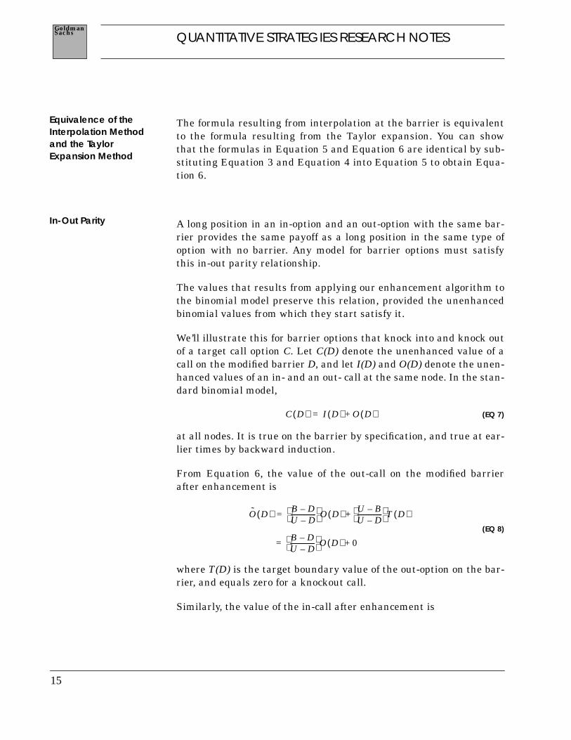
The formula resulting from interpolation at the barrier is equivalentto the formula resulting from the Taylor expansion. You can showthat the formulas in Equation 5 and Equation 6 are identical by sub-stituting Equation 3 and Equation 4 into Equation 5 to obtain Equa-tion 6.

A long position in an in-option and an out-option with the same bar-rier provides the same payoff as a long position in the same type ofoption with no barrier. Any model for barrier options must satisfythis in-out parity relationship.

The values that results from applying our enhancement algorithm tothe binomial model preserve this relation, provided the unenhancedbinomial values from which they start satisfy it.

We’ll illustrate this for barrier options that knock into and knock outof a target call option C. Let C(D) denote the unenhanced value of acall on the modified barrier D, and let I(D) and O(D) denote the unen-hanced values of an in- and an outcall at the same node. In the stan-dard binomial model,

(EQ 7)

at all nodes. It is true on the barrier by specification, and true at ear-lier times by backward induction.

From Equation 6, the value of the out-call on the modified barrierafter enhancement is

(EQ 8)

where T(D) is the target boundary value of the out-option on the bar-rier, and equals zero for a knockout call.

Similarly, the value of the in-call after enhancement is

Equivalence of theInterpolation Methodand the TaylorExpansion Method

In-Out Parity

C D( ) I D( ) O D( )+=

O D( ) B D–U D–----------------

O D( ) U B–U D–----------------

T D( )+=

B D–U D–----------------

O D( ) 0+=

16


(EQ 9)

where T'(D) is the target boundary value of the in-option on the bar-rier, and equals the value C(D) of the call itself.

Adding the above two equations gives

(EQ 10)

where the second line of Equation 10 follows from the unenhancedform of in-out parity in Equation 7, and the last line follows fromsimple algebra. The enhanced binomial values satisfy in-out parity.

I D( ) B D–U D–----------------

I D( ) U B–U D–----------------

T′ D( )+=

B D–U D–----------------

O D( ) U B–( )U D–( )

--------------------C D( )+=

O D( ) I D( )+B D–( )U D–( )

-------------------- O D( ) I D( )+[ ] U B–U D–----------------

C D( )+=

B D–( )U D–( )

-------------------- C D( )[ ] U B–U D–----------------

C D( )+=

C D( )=

17


In this section we illustrate how to implement the method on a sim-ple binomial tree.

Figure 10 contains the stock tree of Figure 3. It corresponds to a nor-mal stock price volatility of 10 points per year, with zero interestrates and zero dividend yields. Also shown are the expiration bound-ary for an up-and-out five-year call on the stock with a strike of 70and a knockout barrier at 125.

A BINOMIAL EXAMPLE

FIGURE 10. An up-and-out call with strike of 70 and out-barrier of 125on a sample binomial tree. The stock is assumed to have a normalprice volatility of 10 points per year, with moves occurring only onceper year. We also assume zero dividend yield and zero interest rates.All transition probabilities on the tree are identical and equal to 1/2.

100

110

130

140

150

130

110110

90

100 100

90 90

80 80

70 70

60

50

strike

specified barrier (125)

tree of stock prices

year 0 1 2 3 4 5

120 120

18


The first tree in Figure 11 shows the unenhanced valuation of the up-and-out call when the barrier is moved up to the effective barrier,according to the first step in our algorithm. The value at each node inyear 5 is the value of the call at expiration. At stock levels of 130 orhigher, the call is knocked-out and therefore worth zero at all nodeson the effective barrier. The option value Cn at any node n inside theeffective barrier and the expiration boundary is computed from thevalues Cu and Cd using the usual binomial discounted expectationsformula with equal probabilities and zero interest rates:

(EQ 11)

The current unenhanced value of the call at the root of the tree isfound to be 17.50.

Now let’s correct the values on the modified barrier to allow for thefact that the specified barrier is actually closer than the effective bar-rier. In the lower tree of Figure 11, in year 4, the real barrier B = 125lies between node U =140 on the effective barrier and node D = 120on the modified barrier. The value of the knockout call at node Dwhen the barrier is at the effective barrier is V(D) = 20; the value ofthe knockout call when the barrier is at the modified barrier is 0(because it knocks out there). In the notation of the interpolation for-mula of Equation 6, the enhanced value of the call option at node D isgiven by

(EQ 12)

The enhanced value at node D in the second tree of Figure 11 is 5,lower than the unenhanced value of 20, because the true barrier iscloser than the effective barrier.

We can use the same formula for interpolating between the U' = 130and D' = 110 nodes in year 3 of Figure 11. The unenhanced value ofthe call at node D' in the upper tree is V(D') = 25. The enhancedvalue is given by

CnCu Cd+

2--------------------=

V D( ) 125 120–( )140 120–( )

---------------------------- 20× 140 125–( )140 120–( )

---------------------------- 0×+=

520------ 20× 15

20------ 0×+=

5=

19


FIGURE 11. Valuing the up-and-out call on the tree of Figure 4.

17.5

17.5 12.5

0

0

0

20

4025

17.5 22.5

30

20 20

12.5

10

5 0

0

0

strike

effective (upper) barrie r

specified barrier

12.5 5

4018.75

20

0

0

15.937530

10

0

20

5

19.375

12.5

15.9375

15.9375

effective (upper) barrier

strike

specified barrier

modified (lower) barrier

unenhanced valuation

enhanced valuation

tree of call prices:

tree of call prices:

year 0 1 2 3 4 5

expiration

expiration

U

D

U'

D'

U

D

U'

D'

boundary

boundary

20


(EQ 13)

This value is again lower than the unenhanced value, because the D'node lies closer to the true barrier than to the effective barrier.

The lower tree of Figure 11 now has payoff values for the up-and-outcall on both the expiration boundary and the modified barrier. We canuse the backward induction formula of Equation 11 to calculate theoption values at all nodes interior to the boundaries. The currentenhanced option value at the root of the tree is found to be 15.94,lower than the unenhanced value of 17.50 found previously.

When interest rates and dividend yields are non-zero, you can useexactly the same methodology to diminish the specification error andso get enhanced values for barrier options. In practice you wouldneed to use trees with about 100 levels rather than 5 or 6.

V D( ) 125 110–( )130 110–( )

---------------------------- 25× 130 125–( )130 110–( )

---------------------------- 0×+=

1520------ 25× 5

20------ 0×+=

18.75=

21


We now present several examples that illustrate the improvementsobtained in using this method, both on binomial trees and on moregeneral lattices.

In Figure 2 we showed the slow convergence of the unenhanced bino-mial method for a one-year European down-and-out call option, withstrike at 100 and barrier at 95, as a function of the number of treelevels. Figure 12 shows the improved convergence of the enhancedvalues. You can see how much more rapidly the enhanced valuesapproach the analytical result as the number of levels increase. Thesawtooth behavior damps out at a faster rate. For numbers of levelsgreater than 80, the result is virtually perfect.

.

In the above example we knew the exact analytic value for theoption, so the enhancement was not really necessary. Now let’s lookat some other examples where the enhancement is importantbecause the analytic solution is unavailable.

THE EFFICACYOF THE ENHANCEMENT

FIGURE 12. Convergence to analytic value of an enhanced binomially-valued one-year European down-and-out call option as the number ofbinomial levels increases. We assume an index level of 100, a strike of100, a barrier level of 95, an annually compounded riskless interestrate of 10% per year, zero dividend yield, and a volatility of 20%. Theanalytic value is 7.31.

Option Value

binomial

enhanced

analytic

levels

10

20

30

40

50

60

70

80

90

10

01

10

12

01

30

14

01

50

16

01

70

18

01

90

20

0

7.00

8.00

9.00

10.00

11.00

22


Figure 13 demonstrates the enhancement obtained for an up-and-outcall with the same interest rates and volatility, but with a barrierthat increases linearly through time from a level of 120 at the start ofthe option’s life to a level of 130 at expiration. Again the enhancedsolution has a much smaller sawtooth amplitude than the plain bino-mial method. Between 90 and 100 tree levels, the magnitude of thesawtooth is about five times smaller for the enhanced solution thanfor the plain binomial solution. There is no known analytic solutionfor this type of barrier, so that an enhanced method saves both com-puting time and provides greater accuracy.

FIGURE 13. Convergence of an enhanced binomially-valued one-yearEuropean up-and-out call option as the number of binomial levelsincreases. We assume an index level of 100, a strike of 100, an annuallycompounded riskless interest rate of 10% per year, zero dividendyield, and a volatility of 20%. The barrier increases linearly with timefrom 120 to 130.

Option Value

binomial

enhanced

levels

40

50

60

70

80

90

10

0

11

0

12

0

13

0

14

0

15

0

16

0

2.50

2.80

3.10

3.40

3.70

4.00

23


Barrier options valued on an implied tree4 in the presence of a gen-eral volatility smile also have no analytic solution. Figure 14 illus-trates the enhancement obtained for an up-and-out call with barrierat 120, but with a volatility skew for the underlying stock. Weassume a skew that varies linearly from an implied volatility of 20%for out-of-the-money puts struck at 60 to an implied volatility of 12%for out-of-the-money calls struck at 140. Once again, the enhancedsolution seems to be converging to the asymptotically correct valuewith much smaller sawtooth fluctuations.

Finally, we stress that this enhancement method works for well-known lattice-based finite difference methods as well as the binomialmethod. Figure 15 shows the effect of our enhancement algorithm onthe value and delta of a down-and-in call with strike at 100 and bar-rier at 95, valued using the implicit (trinomial) finite-difference

4. See Derman and Kani (1994).

FIGURE 14. Convergence of an enhanced binomially-valued one-yearEuropean down-and-out call option as the number of binomial levelsincreases. We assume an index level of 100, a strike of 100, a barrierlevel of 120, an annually compounded riskless interest rate of 10% peryear, zero dividend yield, and a volatility skew that varies linearlyfrom 20%for puts struck at 60 to 12% for calls struck at 140.

Option Value

binomial

enhanced

levels

30 40

50

60

70

80

90

10

0

2.00

2.20

2.40

2.60

2.80

3.00

24


method. The enhancement again leads to a much smoother and morerapidly converging option value and delta.

FIGURE 15. Convergence of an enhanced binomially-valued one-yearEuropean down-and-in call option as the number of lattice levelsalong the stock axis increases. We assume an index level of 100, astrike of 100, a barrier level of 95, an annually compounded risklessinterest rate of 10% per year, zero dividend yield, and a volatility of20%.

-0.65

-0.6

-0.65

-0.5

-0.55

-0.4

De

lta binomialenhanced

3

3.5

4

4.5

5

5.5

6

Va

lue

binomialenhanced

25


REFERENCES

Boyle, Phelim P. Options: A Monte Carlo Approach, Journal of Finan-cial Economics 4 (May 1977), pp. 323-338.Boyle, Phelim P. and S. H. Lau. Bumping Up Against the Barrier withthe Binomial Method, Journal of Derivatives 1 (Summer 1994), pp. 6-14.Cox, John C., Stephen A. Ross and Mark Rubinstein. Option Pricing:A Simplified Approach, Journal of Financial Economics 7 (September1979), pp. 229-263.Derman, Emanuel and Iraj Kani. The Ins and Outs of BarrierOptions, Goldman Sachs Quantitative Strategies Research Notes,June 1993.Derman, Emanuel and Iraj Kani. Riding on a Smile, RISK 7 no 2(1994), pp. 32-39.Bruno Dupire. Pricing with a Smile, RISK 7 no 1 (1994), pp. 18-20.Margrabe, William. Binomial Pricing of Exploding Options, Topics inMoney and Securities Markets, Bankers Trust Company, May 1989,No. 149.R.C. Merton. Theory of Rational Option Pricing, Bell Journal of Eco-nomics and Management Science, 4 (1973), pp. 141-183.Mark E. Rubinstein, Implied Binomial Trees, Journal of Finance, 69(1994), pp. 771-818.

Documents

Quantitative Strategies Research Notesjanroman.dhis.org/finance/Numerical Methods/enhanced_numerical_… · gest a method for enhancing the numerical solution ... See Derman and Kani