Embed Size (px)
Citation preview
Pseudoadiabatic chart / sonde diagram
p
p
cR
cR
pconstT
ppT
⋅⋅=
⎟⎟⎠
⎞⎜⎜⎝
⎛=
θ
θ 0
This can be plotted with a logarithmic scale for the pressure.
The lines for constant potential temperature is following the dry adiabatic lapse rate.
We are most interested in the stippled area in Fig. 2.6.

Temperature – Entropy (pot.temp.) diagramThe chart in Fig. 2.6 may be plotted as a temperature-entropy diagram (Fig. 2.20a).
Again, we are only interested in the atmospheric temperature interval (stippled), which is usually rotated (ca. Fig. 2.20b).
Skew-T – ln p diagram (Fig. 2.20b)

Saturated air
When saturated air is lifted adiabatically, water vapor will condense. All the heat formed in the phase change is assumed to warm the air parcel and the liquid water removed.
The lapse rate for this process is called pseudoatiabatic lapse rate (fuktigadiabat).
It is a good idea to plot both adiabats in the same diagram!
And they are, as a function of pressure and temperature in the chart in the back of the book.
Also plotted are the saturated mixing ratios at given T and p.
dTdw
cLdz
dTs
p
ds
+
Γ=−=Γ1

Stability
Why do we want both adiabats in the same chart?
Because dry/unsaturated air follows the dry adiabat, while saturated air follows the moist (pseudo) adiabat.

( )Γ−Γ= dTdzd 11 θ
θ
0
0
0
>
=
<
dzddzddzd
θ
θ
θ Unstable
Neutral
Stable
Unsaturated air Saturated air
Condensing water will free energy: dq = -Ldws
Where L is latent heat, and dws is the amount condensed.
But we have
And it can be shown (Ex.2.33) that
So that
spp
dwTc
LTc
dqd −==θθ
⎟⎟⎠
⎞⎜⎜⎝
⎛=
TcLwddw
TcL
p
ss
p
⎟⎟⎠
⎞⎜⎜⎝
⎛=+=−
ep
s constTc
Lwθθθ lnln
es Tw θθ →⇒→ 0/
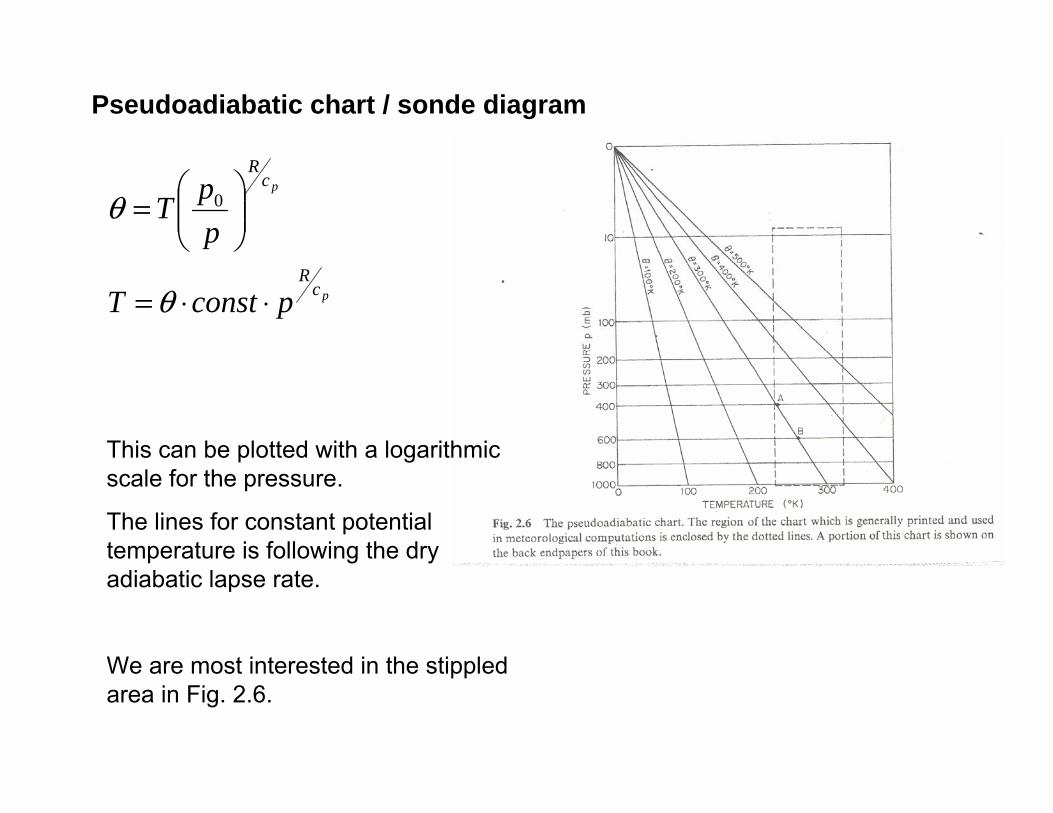
Convective instability
We have convective instability when
0<dzd eθ
0<dz
d wθ
or when
Conditional instability
We have conditional instability when
ds Γ<Γ<Γ
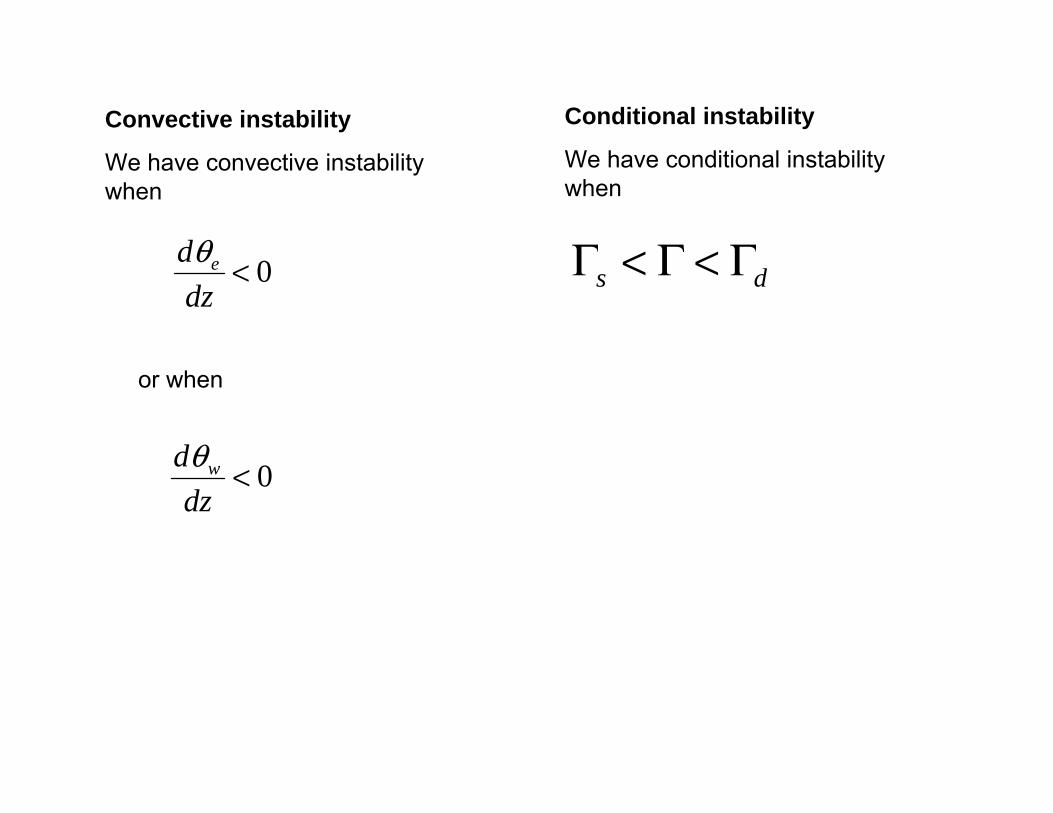
The Amble sonde diagram1050hPa – 500hPa: Skew-T – ln p diagram
500hPa – 20hPa: Skew-T – p diagram
Moist adiabatDry adiabatTemperatureSat. mix. rat.
Pot.temp. on the dry adiabat
Pressure
Thickness of layer
Height of the standard atmosphere

Exercise 2.48Pressure 200hPa, temperature T=-60˚C. Find the potential temperature using a sonde diagram.
200hPa
T=-60˚C
θ =70˚C
θ =60˚C
Approximately θ =66˚C
CKKppT
pcR
o64337200
10002131004
287
0 ==⎟⎠⎞
⎜⎝⎛×=⎟⎟
⎠
⎞⎜⎜⎝
⎛=θ

Exercise 2.49ap=1000hPa
T=15˚C
Td=4˚C
Mixing ratio (w)Relative humidity (RH)Potential temperature (θ)Wet-bulb temperature (Tw)Wet-bulb potential temperature (θw)
TTd
ws(Td) ws(T)
Dew point temperature
The final temperature when cooling air at constant pressure untill it is saturated.
The saturated mixing ratio at Td is then the mixing ratio of the air.
w(T) = ws(Td) = 5.1g/kg
Must NOT be confused with saturated mixing ratio at T: ws(T).
Relative humidity
RH = 100% w(T)/ws(T)
= 100% ws(Td)/ws(T)
= 100% x 5.1/10.8
= 47%
Potential temperature
We are at 1000hPa, so
θ = T = 15˚C
Wet-bulb temperature
The temperature we get after evaporating water into the air until saturation.
This is easily done on this chart, lifting the air along the dry adiabat until saturation, and then along the pseudoadiabat on its way down.
Tw = θw = 9.3˚C

Exercise 2.49bp=1000hPa
T=15˚C, Td=4˚C
Lift the air to 900hPa.
T
Td(900hPa)
ws(Td) ws(T)
900hPa
w = 5.1g/kgRH = 100% x 5.1/6.8 = 73%θ = 15˚C as before. (Conserved)Tw = 4.7˚Cθw = 9.3˚C as before. (Conserved)
Td Tw
Tw(900hPa)

Exercise 2.49cp=1000hPa
T=15˚C, Td=4˚C
Lift the air to 800hPa.
T
ws(Td) ws(T)
Td Tw
ws(Td(800hPa)
w = 4.4g/kgRH = 100% x 4.4/4.4 = 100%θ = 17˚C. (Not conserved for moist adiabatic processes)Tw = -1˚Cθw = 9.3˚C as before. (Conserved)
800hPa

How to find different properties on the chart
Potential temperature: Follow the dry adiabat to 1000hPa and read off the temperature.
Mixing ratio: At the dew point temperature, follow the lines for constant water vapor content downwards.
Saturation mixing ratio: At the actual temperature, follow the line for wdownwards.
Wet-bulb temperature: Follow the dry adiabat from the actual pressure upwards until saturation (the lifting condensation level), and then downwards along the moist adiabat to the starting pressure level.
Wet-bulb potential temerature: From the wet-bulb temperature, follow the moist adiabat to 1000hPa.
Equivalent potential temperature: Lift the parcel to saturation, and then along the moist adiabat until there is no water vapor left (where only the dry adiabat is plotted), and then downwards along the dry adiabat.
Static stability: Look at the lapse rate compared to the dry adiabat. Or look at potential temperature. Stable means θincrease with height.
Conditional instability: If the lapse rate is between the dry and the moist adiabat, we have conditional instability.
Level of free convection: In case of conditional instability only. Lift the parcel to saturation, and upwards along the moist adiabat.

Convective instable air: If θe or θw decreases with height.
When this occurs, an initially stable layer will destabilize as it is lifted, since the top of the layer will cool faster than the bottom, thereby steepening the lapse rate. In reality, whole layers may not be lifted at once; instead, parcels often lift from the boundary layer to their level of free convection (LFC) to form thunderstorms. Thus, the physical process that potential instability represents may or may not occur often during convection.
However, θe (which is more sensitive to moisture than temperature) decreasing with height IS important, since it represents the presence of dry air above moist air which enhances downburst and possibly hail potential if thunderstorms develop.
http://www.crh.noaa.gov/lmk/soo/docu/indices.php

T
ws(T2) ws(T)
Td
T2
Td = 13.9˚CLiquid water: ws(T)-ws(T2) = 10-6 = 4g/kgLose 80% of water: w=10-0.8*4 = 6.8g/kgT(900hPa) = 19.5˚C
700hPa
Exercise 2.52p=1000hPa
T=20˚C
w=10g/kg
Air is lifted when passing a mountain to 700hPa.