Journal of Pharmacokinetics and Biopharmaceutics, Vol. 1, No. 2, 1973

Properties of the Miehaelis-Menten Equation and Its Integrated Form Which Are Useful in Pharmacokinetics

John G. Wagner 1'2

Received Feb. 3, 1972 Final Aug. 7, 1972

Some old equations are reviewed and some new equations have been derived which indicate certain properties of the Michaelis-Menten equation and its integrated forms. Simulated data which obey Michaelis-Menten kinetics have been plotted in various ways to illustrate special relationships. An equation is derived which accurately estimates the slope of the apparently linear decline (ko) of concentrations from the values of Co, Kin, and V m. This indicates the hybrid nature of k o. It is pointed out that if a metabolite is formed by Michaelis-Menten kinetics, then (a) one would not expect linear plots of cumulative amount of metabolite excreted in the urine vs. time, and (b) the plasma clearance of the drug will change with dose, and the plasma clearance of the drug would be expected to be different following administration of the same dose in a rapidly available and a slowly available dosage form. The distortion in parameter values when data arising from M ichaelis-Menten kinetics are evaluated by classical linear pharmacokinetics is indicated.

KEY WORDS: Michaelis-Menten kinetics; dose:dependent kinetics; elimination half-life; areas under blood level curves : urinary excretion of metabolites.

INTRODUCTION

Classical linear pharmacokineties are based on two principal assump- tions: (a) tissues can take up an infinite amount of drug, and (b) drug elim- ination from the body obeys first-order kinetics. Neither of these assumptions is strictly valid even after administration of low doses of a drug, but the discrepancy between the assumptions and the facts becomes very evident when the same drug is studied in the same species following several different doses.

This report is concerned with certain properties of the Michaelis- Menten equation (1, 2) and its integrated form (3, 4), which together with

1 College of Pharmacy and Upjohn Center for Clinical Pharmacology, The University of Michigan, Ann Arbor, Michigan 48104.

2 Address requests for reprints to Dr. John G. Wagner, Upjohn Center for Clinical Pharmacology, The University of Michigan, Ann Arbor, Michigan 48104.

103

�9 1973 Plenum Publishing Corporation, 227 West 17th Street, New York, N.Y. 10011.

104 Wagner

appropriate tissue-binding equations (5-8) appear to explain observed data adequately. This will be illustrated in future publications.

Despite the wide use of the Michaelis Menten equation in enzyme kinetics and its use, since the paper of Lundquist and Wolthers (9), in pharma- cokinetics, the properties of the function appear to be poorly understood. This is mainly due to the fact that most authors have only used the equation in its differential form and are not familiar with C, t data derived from the function. There also seems to be the widespread concept that during an enzyme reaction in which a metabolite is formed the enzyme suddenly becomes "sa tura ted" as the substrate concentration is increased. The Michaelis Menten equation is shown as equation 1 :

v = - d C / d t = VmC/(K,, + C) (1)

where v is the overall velocity of the reaction, V m is the maximum velocity, K m is the so-called Michaelis-Menten constant, C is the substrate con- centration, and t is time. It is obvious from equation 1 that when C >> K m,

the velocity only approaches V,, but v = V m only when C approaches in- finity. Analogously, the fact that first-order drug elimination is usually an approximat ion to the Michaelis-Menten equation was apparently first pointed out by Rescigno and Segre (4). The apparent first-order rate constant for drug elimination, when a single metabolite is formed, is an approximation of the ratio V,,/K,, , but this value is never really reached until C reaches zero. Mathematically, it is more appropriate to write K ~ V,,/Km as C ~ 0. Lundquist and Wolthers (9) discussed certain properties of equation 1. These were (a) C = K m when v = Vm/2, and (b) v is a maximum when d2v/dt 2 = 0; this corresponds to v = Vm/3 and C = Kin~2.

The integrated form of equation 1 may be written as equation 2 :

C 1 - - C 2 --]- K,, In (C1/C2) = Vm(t 2 - gl) (2)

where C 1,q and C2,t 2 a r e any two points on the C,t curve. In a special case, one may write C 1 = Co where C o = C when t = 0. The author is suggesting that in the absence of tissue binding of drug, terminal blood or plasma concentration data should often be fitted to equation 2 rather than to the classical first-order equations shown as equations 3 and 4 :

C = Co e -K' (3)

l n C = l n C o - K t (4)

Kri iger-Thiemer (10) pointed out that deviations from linearity in pharmacokinetics may occur due to the absorption process, due to dis- tribution, due to tissue binding of the drug, due to metabolic processes, and

Properties of the Michaelis-Menten Equation 105

due to excretory processes. Krtiger-Thiemer and Levine (11) discussed several pharmacokinetic models involving Michaelis-Menten elimination kinetics, particularly one which comprises all characteristics of enzymatic processes, namely, reversibility, saturability, and substrate depletion.

THEORY

The Pseudolinear Phase

If equation 1 is integrated between the limits C = 0 to C = Co, one obtains equation 5 :

Co - C + K m In (Co/C) = V,,t (5)

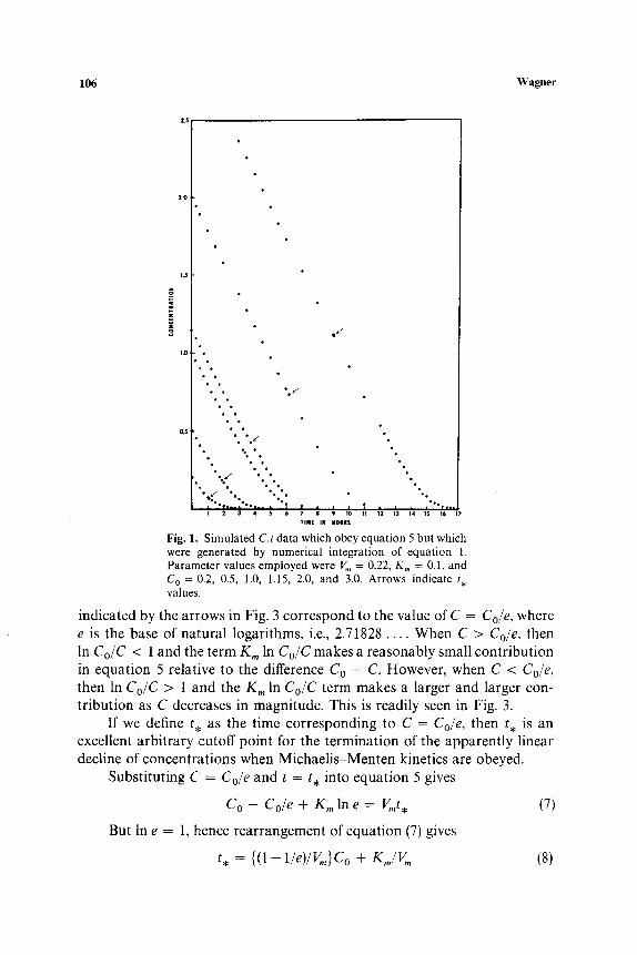
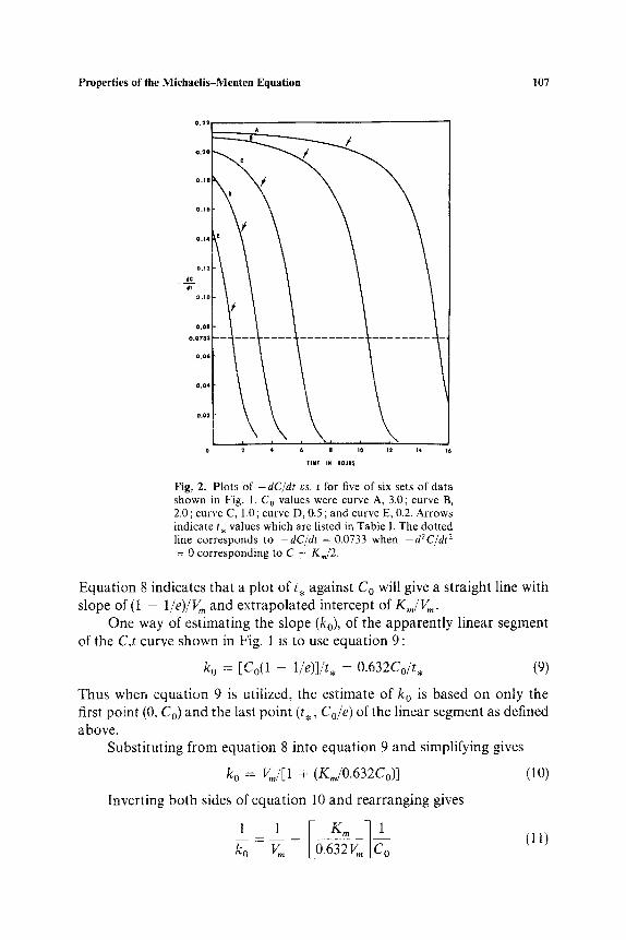
where C = Co at t = 0. It is interesting that Henri (3) published equation 5 in 1902 before Michaelis and Menten (1) published equation 1 in 1913. Plots of C vs. t, generated with equation 5 or by numerical integration of equation 1, as illustrated in Fig. 1, have a "hockey-stick" shape. Each curve has an apparently (but not actually) linear segment. The latter is emphasized by Fig. 2, which shows plots of - d C / d t vs. t for five of the six sets of data shown in Fig. 1. The arrows on both Figs. 1 and 2 designate certain times, which may be symbolized by t . . It should be noted that a plastic ruler placed over the curves in Fig. 1 in the intervals 0 _< t _< t . shows them to be essentially linear to the eye, but beyond the arrows, designating the t . values, there is noticeable curvature. This pseudolinear phase is evident in Fig. 1 despite the nonconstancy of the - dC/dt vs. t curves in the same intervals as seen in Fig. 2. A possible approach to show the deviation in linearity would be to rearrange equation 1 as shown in equation 6:

- d C / d t = Vm/[1 + (Km/C)] (6)

Equation 6 suggests that when C is large relative to K m, such that Km/C is small, then the slope of the C,t curve will be relatively constant. However, this approach suggests that if one chose some arbitrary value, such as C <_ 2K m or Km/C >_ 0.5, then one would predict that the end of the pseudo- linear phase would always correspond to the same value of C, independent of the Co value. A careful appraisal of the curves shown in Fig. 1 with a plastic ruler, as indicated above, will indicate that this situation does not hold.

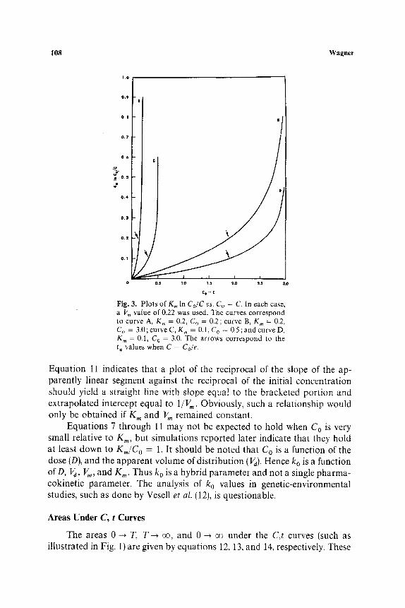
To meet the linearity requirement, the second term on the left-hand side of equation 5 must be small relative to the first term. Figure 3 is a plot of the second term, K~ In Co~C, against the first term, C o - C, for C,t data gener- ated from four representative combinations of C o, V,,, and K,,. The points

106 Wagner

1.5

2 5

2 0 -

I o . .

0 ,5 - �9

, � 9 1 4 9 1 7 6 1 4 9 1 4 9 �9 ~ I 2 3 4 5 6

~

t j

2 �9 ~ L � 9 1 4 9 1 4 9

TIME IN HOURS

Fig. 1. Simulated C,t data which obey equation 5 but which were generated by numerical integration of equation 1. Parameter values employed were V m = 0.22, K,, = 0.1, and C o = 0.2, 0.5, 1.0, 1.15, 2.0, and 3.0. Arrows indicate t , values.

indicated by the arrows in Fig. 3 correspond to the value of C = Cole, where e is the base of natural logarithms, i.e., 2.71828 . . . . When C > Co~e, then In Co/C < 1 and the term Km in Co/C makes a reasonably small contribution in equation 5 relative to the difference Co - C. However, when C < Cole, then In Co/C > 1 and the Km In Co/C term makes a larger and larger con- tribution as C decreases in magnitude. This is readily seen in Fig. 3.

If we define t , as the time corresponding to C = Cole, then t , is an excellent arbitrary cutoff point for the termination of the apparently linear decline of concentrations when Michaelis-Menten kinetics are obeyed.

Substituting C = Cole and t = t , into equation 5 gives

Co - Co/e + K,, In e = Vmt , (7)

But In e = 1, hence rearrangement of equation (7) gives

t , = { (1 - 1/e)/Vm}C o + K,,/V m (8)

Properties of the Michaelis-Menten Equation 107

0 2 4 6 H 10 12 14 16

TIME IN HOURS

Fig, 2. P lo t s of - dC/dt vs. t for five of six sets of da t a shown in Fig. 1. C o values were curve A, 3.0; curve B, 2.0; curve C, 1.0; curve D, 0.5 ; and curve E, 0.2. Ar rows ind ica te t , va lues which are l isted in Tab le I. The do t ted line co r r e sponds to - d C / d t = 0.0733 when -dZC/d t 2 = 0 co r r e spond ing to C = K,,/2.

Equation 8 indicates that a plot of t , against Co will give a straight line with slope of (1 - 1/e)/Vm and extrapolated intercept of K,,/Vm.

One way of estimating the slope (ko), of the apparently linear segment of the C,t curve shown in Fig. 1 is to use equation 9 :

k 0 = ECo(1 - 1/e)]/t , = 0 .632Co/t , (9)

Thus when equation 9 is utilized, the estimate of k 0 is based on only the first point (0, Co) and the last point (t , , Cole) of the linear segment as defined above.

Substituting from equation 8 into equation 9 and simplifying gives

k o = Vm/[1 + (Km/0.632Co) l (10)

Inverting both sides of equation 10 and rearranging gives

1 , F K m ] I ko - V,, + LO.632vmJCo (11)

108 W a g n e r

0,9 - j

0 . | -

O.Y

0 . 6

~_~O.S

J

0.4

0.3

0.2 -~ /

r I

D

0.5 1.0 1~5 2.0 2,5 3,0

Co-C

Fig. 3. P l o t s o f K,~ In C U C vs. Co - C. In e a c h case , a V,. v a l u e o f 0 .22 w a s used . T h e c u r v e s c o r r e s p o n d to c u r v e A, K m = 0.2, C O = 0.2; c u r v e B, K, , = 0.2, C o = 3.0 ; c u r v e C, K , , = 0.1, C o = 0.5 ; a n d c u r v e D, K , . = 0.1, C o = 3.0. T h e a r r o w s c o r r e s p o n d to the t , v a l u e s w h e n C = Co/e.

Equation l l indicates that a plot of the reciprocal of the slope of the ap- parently linear segment against the reciprocal of the initial concentration should yield a straight line with slope equal to the bracketed portion and extrapolated intercept equal to 1/V m. Obviously, such a relationship would only be obtained if K,, and V,, remained constant.

Equations 7 through 11 may not be expected to hold when Co is very small relative to K,,, but simulations reported later indicate that they hold at least down to Kin/Co = 1. It should be noted that Co is a function of the dose (D), and the apparent volume of distribution (Vd). Hence k o is a function of D, Va, Vm, and K,,. Thus ko is a hybrid parameter and not a single pharma- cokinetic parameter. The analysis of k 0 values in genetic-environmental studies, such as done by Vesell et al. (12), is questionable.

Areas Under C, t Curves

The areas 0-~ T, T ~ ~ , and 0-~ ~ under the C,t curves (such as illustrated in Fig. 1) are given by equations 12, 13, and 14, respectively. These

Properties of the Michaelis-Menten Equation 109

equations were readily obtained by appropriate integration from equation 5. They apply only to the pharmacokinetic situation where only one metabolite is formed according to the kinetics of Michaelis and Menten, and they assume a one-compartment open model.

Area 0 --, T

Area T-~ vo =

= C . d t = t . d C T

{ tl + - C o C r + K m C o - C r C r l n c r (12)

f; f) C . d t = t . d C

Vm L o ~ +Kin l n ~ r + 1

Area 0 -~ ~ . = C . d t = t . d C = K, , [~ 2 + K m

(13)

(14)

Urinary Excretion of a Metabolite When the Metabolite is Formed According to the Kinetics of Michaelis and Menten

In general, one may write (5)

Rate of Rate due to Rate due to urinary = glomerular + active tubular -

excretion filtration secretion

metabolite formed For a by equation 15 in mathematical form as in equation 16 :

Rate due to tubular (15)

reabsorption

Michaelis-Menten kinetics, one may write

In equation 16, d a f t & is the rate of urinary excretion of the metabolite, c~ is the fraction of the total drug in plasma which is free (non-protein-bound), k 1 and kap p a r e first-order constants, Va is the appropriate volume of dis- tribution of the metabolite, C is the plasma concentration of the metabolite, T,, is the transport maximum, K m is the Michaelis constant of the transport mechanism, V~ is the effective volume of the tubule fluid from which re- absorption occurs, and Cu is the urine concentration of the metabolite. The quantity k I V a is equivalent to the glomerular filtration rate.

TmC d A u / d t = ~ k l VaC + K m + C kapp" V r C, (16)

110 Wagner

When the transport mechanism is in the first-order region (i.e., K,, >> C), then equation 16 simplifies to equation 17 :

d A , / d t = Va[kxeC + k2C ~ - k a p p �9 V T . C u (17)

where k z = T'~/K~ and T~, = Tm/V d. At constant pH of tubule fluid, k,pp will be a constant. If there is no reabsorption of metabolite, then equation 17 simplifies to equation 18 :

d A , / d t = VdC[k,~ + k23 (18)

If there is only glomerular filtration of metabolite, then equation 19 applies :

dAu/dt = kx~VdC (19)

When metabolite is formed by the kinetics of Michaelis and Menten, then the C in equations 16 through 19 is the C in equation 1 or 5. All of these equations indicate a nonlinear relationship between dAu/dt and C or dAu/dt and t. Hence, if real excretion rate, time plots, and plots of cumulative amounts of metabolite excreted vs. time are apparently linear, true linearity is not supported by the above equations.

Methods for Obtaining Preliminary Estimates of V m and/~

Lundquist and Wolthers (9) described a method to obtain preliminary estimates of the parameters V m and Km from a set of alcohol blood levels. Two additional methods are described below :

M e t h o d 1

One chooses three points, ( C l , t l ) , (C2,t2) , and (C3,ta) , from the set of observed C,t values, or one draws a smooth line through the observed set of Cot values and takes three values from the smooth line. In relation to Fig. 1, one point should be at or near the top of the apparently linear portion, one point should be at or near the bottom of the apparently linear portion, and the third point should be near the bottom of the curved "foot" of the "hockey stick." One then writes two equations analogous to equation 2 as indicated by equations 20 and 21, The numerical values of C1, C2, C3, tl , t2, and t3 are substituted into

C1 - C2 + K,, In (C~/Cz) = V,,(tz - t l) (20)

C1 - C a + K m In (C1/C3) = V,,(t a - t~) (21)

Hence one has two equations with two unknowns, namely, V,, and Kin, and by the process of elimination can obtain one unknown; then by substitution into one of the equations, one can obtain the other unknown.

Properties of the Michaelis-Menten Equation i 11

Method 2

The derivatives of equation 1 are approximated from the observed data by - A C / A t values, and the C values are approximated as the mid- points of the AC values. Rearrangement of equation 1 yields equation 22:

- A C / d t - Vm + C (22)

Equation 22 is the equation of a straight line. When C / ( - A C / A T ) is plotted against C, the intercept of the line corresponding to C = 0 is Km/Vm and the slope of the line is 1/Vm. Hence from the values of the slope and the intercept, the estimates of Vm and K m may be obtained.

Estimates of Vm and K,, obtained by methods l and 2 should be con- sidered as only preliminary estimates which are good enough to start a computer iterating. The observed set of C,t data should then be fitted by the method of least squares.

EXPERIMENTAL

Generation of Simulated C, t Data

Simulated C,t data obeying equation 5 were generated by assigning numerical values to C o, V,,, and Km using the program NONLIN and IBM 360/67 computer. Two different approaches were taken: (a) equation 1 was employed and it was numerically integrated by the computer using the Runge-Kutta method which is part of the program NONLIN ; (b) equation 5 was employed in conjunction with a special "root-finder" subroutine. For a given set of parameters, C o, K m, arid V,,, both methods gave the same C values for a given set of t values. In the same manner, observed C,t data may be fitted to equation 5, or terminal blood concentration may be fitted to equation 2, using either of the above methods. Again, both methods give essentially the same estimated values of the parameters Co, V,,, and K m from a given set of C,t data. In addition, the author has programmed a Hewlett- Packard electronic calculator to numerically integrate equation 1 by the Runge-Kutta method, and for a given set of parameter values this method produced the same C,t values as the large digital computer. In all the simu- lations, the step height used was 0.01 hr, and the accuracy in the C values was at least four decimal places.

Most of the simulations were performed with V,, = 0.22, K m = 0.1, and C O = 0.1, 0,2, 0.5, 1.0, 1.15, 2.0, and 3.0. These values of V,, and K,, are those which have been reported (9,13) for alcohol metabolism in man. Other simulations were performed with V,, = 0.22, K,, = 0.2, and Co = 0.2 and

112 Wagner

3.0. Analogous to real alcohol blood levels, V,, has dimensions of mg/ml • hr) and Km and C have dimensions of mg/ml. A Co value of 1.0 or 1.15 in the simulations provides C values roughly equivalent to alcohol blood levels observed in man after a dose of 60 ml of 95 % alcohol (12).

Equation for Apparently Linear Segment of C, t Curves

In the interval 0 _< t _< t , for each set of simulated C,t data, the data were fitted to equation 23 by the method of least squares :

C = C'o - ko t (23.)

Percent Saturation Corresponding to C O

The percent saturation corresponding to C is readily obtained from re- arrangement of equation 1 shown as equation 24 :

- d C / d t IOOC Percent saturation - x 100 - - - (24)

vm K,.+C

RESULTS

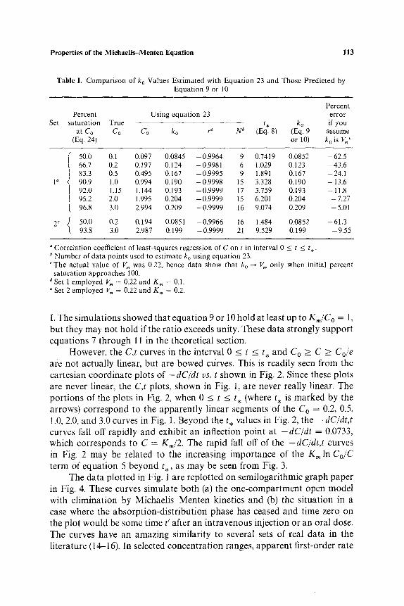
The C,t data generated as described in the experimental section by assigning values of V,, = 0.22, K,, = 0.1, and C o = 0.2, 0.5, 1.0, 1.15, 2.0, and 3.0 are plotted in Fig. 1 on cartesian coordinate graph paper. All curves have a similar shape. The plots are apparently (but not actually) linear for about two thirds of their length, i.e., from Co to Cole, equivalent to going from C o to 0,368Co. When t > t . , there is noticeable curvature. The parameters C~ and k 0 of equation 23 obtained from each set of C,t data in the interval 0 _< t < t . by the method of least squares are shown in Table I along with the correlation coefficients (r), the true Co values, the percent saturation at C o, and the percentage error made if one assumed that k o was equivalent to Vm. It may be seen that none of the k o values is equal to V m. Also, the smaller the value of Co, the smaller the value of k0 and the greater the deviation from the value of V m. Yet, even at low C o values, very high cor- relation coefficients are obtained. In addition, k o ~ V,, as Co ~ ~ . These clata illustrate clearly that when a real alcohol blood or plasma concentration time plot is apparently linear, one cannot conclude that the alcohol is being oxidized at the maximum rate! Goldstein (13) has pointed out that when the blood alcohol concentration falls from 4mg/ml to 0.5 mg/ml, the enzyme would be about 98 % saturated initially and 83 % finally, and the kinetics would appear to be virtually zero order (linear) through this range.

The data in Table I also show that equation 9 or 10 predicts ko essentially exactly, This is seen by comparing the k o values in columns 5 and 9 of Table

Properties of the Miehaelis-Menten Equation 113

Table I. Comparison of k o Values Estimated with Equation 23 and Those Predicted by Equation 9 or 10

Set

Percent Percent Using equation 23 error

saturation True t , k o if you at C O C O C'o ko r ~ N b (Eq. 8) (Eq. 9 assume

(Eq. 24) or 10) k o is V~'

1 d

2 e

50.0 0.1 0.097 0.0845 - 0.9964 9 0.7419 0.0852 - 62.5 66.7 0.2 0.197 0.124 -0.9981 6 1.029 0.123 -43 .6 83.3 0.5 0.495 0.167 -0.9995 9 1.891 0.167 -24.1 90.9 1.0 0.994 0.190 -0.9998 15 3.328 0.190 -13.6 92.0 1.15 1 . 1 4 4 0.193 -0.9999 17 3.759 0.193 -11.8 95.2 2.0 1.995 0.204 - 0.9999 15 6.201 0.204 - 7.27 96.8 3.0 2.994 0.209 -0.9999 16 9.074 0.209 -5.01

50.0 0.2 0.194 0 .0851 -0.9966 16 1 . 4 8 4 0.0852 -61.3 93.8 3.0 2.987 0.199 -0.9999 21 9.529 0.199 -9.55

"Correlation coefficient of least-squares regression of C on t in interval 0 b Number of data points used to estimate ko using equation 23. c The actual value of V,, was 0.22, hence data show that ko --* V,, only

saturation approaches 100. Set 1 employed V,, = 0.22 and K,, = 0.1. Set 2 employed I,~, = 0.22 and K m = 0.2.

< _ t < _ t , .

when initial percent

I. The simulations showed that equation 9 or 10 hold at least up to Km/C o = 1, but they may not hold if the ratio exceeds unity. These data strongly support equations 7 through 11 in the theoretical section.

However, the C,t curves in the interval 0 < t < t , and Co >_ C >>_ Cole are not actually linear, but are bowed ct/rves. This is readily seen from the cartesian coordinate plots of - d C / d t vs. t shown in Fig. 2. Since these plots are never linear, the C,t plots, shown in Fig. 1, are never really linear. The portions of the plots in Fig. 2, when 0 < t _< t , (where t , is marked by the arrows) correspond to the apparently linear segments of the Co = 0.2, 0.5, 1.0, 2.0, and 3.0 curves in Fig. 1. Beyond the t , values in Fig. 2, the - dC/dt,t curves fall off rapidly and exhibit an inflection point at - d C / d t = 0.0733, which corresponds to C = Kin~2. The rapid fall off of the -dC/d t , t curves in Fig. 2 may be related to the increasing importance of the K,, In Co/C term of equation 5 beyond t , , as may be seen from Fig. 3.

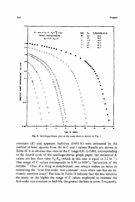
The data plotted in Fig. 1 are replotted on semilogarithmic graph paper in Fig. 4. These curves simulate both (a) the one-compartment open model with elimination by Michaelis-Menten kinetics and (b) the situation in a case where the absorption-distribution phase has ceased and time zero on the plot would be some time t' after an intravenous injection or an oral dose. The curves have an amazing similarity to several sets of real data in the literature (14-16). In selected concentration ranges, apparent first-order rate

114 W a g n e r

10.0

|

0.01

0.001

L C,1 data mf Oa-C+Kml l l~=Vmt

Platted Semilo|aritkmically Ym = 0.22, Im = 0.1

3 . 0 ' 0 0 0 0

2.0 O 0 0

O O O O 0

Ooo o zxz~

0"51 O0 V~7 (3 ~ s ~7 D D LXz~

V~7 O z~ ~7 [3 z~

0.2 ~ ~ o

0 0 ~ o

0 0 0 0 0 0 O

o.1 0

0 ~

0 ~7

0 ~

0 '7

0

I 1 2 4

Ood__t 01L % $aturatin at C o

�9 3.0 96,8 (9 2.0 95.2

1.15 92.0 0 1.0 90, 9 v 0.5 $3,3 0 0.2 66.7

O0 �9

0 0

0

0

% o

o

o

~ o o

D & D & 0 Q & D

& O

& 0 0 D O & O & D & O & Q

D V D

I I I 6 $ 10

TIM[ IN NOUlI

%%%

o

o

o

o

o

I I 12 14

Fig . 4. S e m i l o g a r i t h m i c p l o t o f the s a m e d a t a as s h o w n in Fig . 1.

0

I 16 111

constants (K) and apparent half-lives (0.693/K) were estimated by the method of least squares from the In C and t values. Results are shown in Table II. It is obvious that even in the C range 0.01 to 0.001, corresponding to the fourth cycle of the semilogarithmic graph paper, the estimated K values are less than ratio Vm/K,, (which in this case is equal to 2.2 hr-1). This range of C values corresponds to 0.99 to 9 . 0 9 ~ "saturation of the enzyme." Thus, if a drug is metabolized, one always makes an error in estimating the "true first-order rate constant" even when one has an ex- tremely sensitive assay! The data in Table II indicate that the less sensitive the assay, or the higher the range of C values employed to estimate the first-order rate constant or half-life, the greater the bias or error. Frequently,

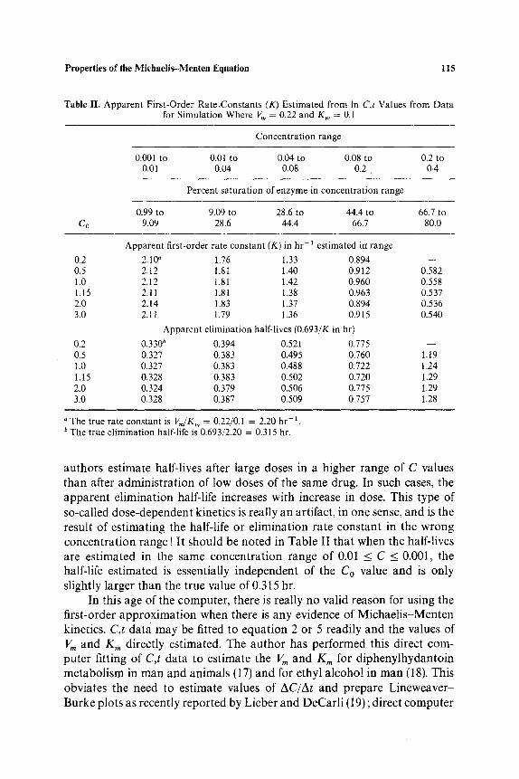
Properties of the Miehaelis-Menten Equation 115

Table II. Apparent First-Order RateoConstants (K) Estimated from In C,t Values from Data for Simulation Where V,, = 0.22 and K,, = 0.1

Concentration range

0.001 to 0.01 to 0.04 to 0.08 to 0.2 to 0.01 0.04 0.08 0.2 0-4

Percent saturation of enzyme in concentration range

0.99 to 9.09 to 28.6 to 44.4 to 66.7 to Co 9.09 28.6 44.4 66.7 80.0

Apparent first-order rate constant (K) in h r - 1 estimated ir~ range

0.2 2.10" 1.76 1.33 0.894 - - 0.5 2.12 1.81 1.40 0.912 0.582 1.0 2.12 1.81 1.42 0.960 0.558 1.15 2.11 1.81 1.38 0.963 0.537 2.0 2.14 1.83 1.37 0.894 0.536 3.0 2.11 1.79 1.36 0.915 0.540

Apparent elimination half-lives (0.693/K in hr)

0.2 0.330 b 0.394 0.521 0.775 - - 0.5 0.327 0.383 0.495 0.760 1.19 1.0 0.327 0.383 0.488 0.722 1.24 1.15 0.328 0.383 0.502 0.720 1.29 2.0 0.324 0.379 0.506 0.775 1.29 3.0 0.328 0.387 0.509 0.757 1.28

a The true rate constant is V,,/K,~ = 0.22/0.1 = 2.20 h r - 1. b The true elimination half-life is 0.693/2.20 = 0.315 hr.

authors estimate half-lives after large doses in a higher range of C values than after administration of low doses of the same drug. In such cases, the apparent elimination half-life increases with increase in dose. This type of so-called dose-dependent kinetics is really an artifact, in one sense, and i3 the result of estimating the half-life or elimination rate constant in the wrong concentration range ! It should be noted in Table II that when the half-lives are estimated in the same concentration range of 0.01 __<_ C < 0.001, the half-life estimated is essentially independent of the Co value and is only slightly larger than the true value of 0.315 hr.

In this age of the computer, there is really no valid reason for using the first-order approximation when there is any evidence of Michaelis-Menten kinetics. C,t data may be fitted to equation 2 or 5 readily and the values of V,, and K,, directly estimated. The author has performed this direct com- puter fitting of C,t data to estimate the V,, and K,, for diphenylhydantoin metabolism in man and animals (17) and for ethyl alcohol in man (18). This obviates the need to estimate values of AC/At and prepare Lineweaver- Burke plots as recently reported by Lieber and DeCarli (19) ; direct computer

116 Wagner

fitting is also more accurate and provides standard deviations of the esti- mated K,, and V,, values which are not obtainable when graphical methods are used. Direct computer fitting also obviates the need for various approx- imations of the integrated rate equation (equation 5) as discussed by Morgan (20)--except where these approximations may be used to obtain preliminary estimates of parameters to start the computer iterating.

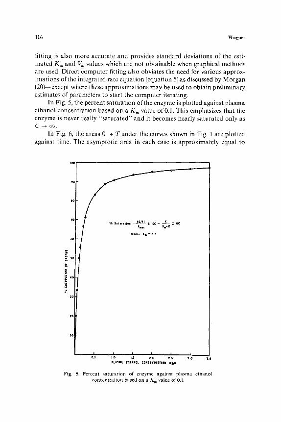
In Fig. 5, the percent saturation of the enzyme is plotted against plasma ethanol concentration based on a K m value of 0.1. This emphasizes that the enzyme is never really "saturated" and it becomes nearly saturated only as C --* oo.

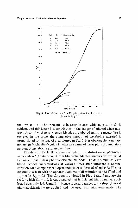
In Fig. 6, the areas 0 --* T under the curves shown in Fig. 1 are plotted against time. The asymptotic area in each case is approximately equal to

100

H

DO

70 X lOO

vRa x I~§

w h e r e Hm~ 0.1 6 0

R 50

4o

3o

2o

lO

I I I I I I O,S 1.0 1.5 ~.0 2,5 3,0 3,5

PLASMA ETHANOL COHC[IITI&TIOII, im|/ i l

Fig. 5. Percent saturat ion of enzyme against plasma ethanol concentration based on a K m value of 0.1.

Properties of the Michaelis-Menten Equation 117

22

20

18

16

14

12

Code 0 o % S a t u r a t i H mt g e

I ) 3 . 0 96.B

O 2 .0 95 .2

1.15 92 .0

(] 1.0 90 .9

~ ' 0.5 83 .3

Km = 0.1, Ym = 0.22

2 4 6 II 10 12 14 16

'TIM[ IN HOURS

Fig. 6. Pl0t of the area 0 -~ T against time for the curves plotted in Fig. 1.

the area 0 --, oo. The tremendous increase in area with increase in Co is evident, and this factor is a contr ibutor to the danger of ethanol when mis- used. Also, if Michaelis-Menten kinetics are obeyed and the metabolite is excreted in the urine, the cumulative amount of metabolite excreted is proport ional to the type of area plotted in Fig. 6. It is obvious that one can- not assign Michaelis-Menten kinetics as a cause of linear plots of cumulative amount of metabolite excreted vs. time.

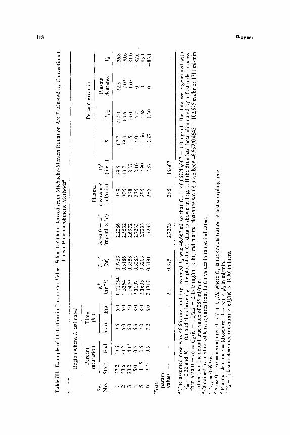
The data in Table III are an example of the distortion in parameter values when C,t data derived from Michaelis-Menten kinetics are evaluated by conventional linear pharmacokinet ic methods. The data simulated were blood alcohol concentrations at various times after intravenous admin- istration (one-compartment open model) of a dose of 60 ml (46.667 g) of ethanol to a man with an apparent volume of distribution of 46,667 ml and V m = 0.22, K m = 0.1. The C,t data are plotted in Figs. 1 and 4 and are the set for which C o = 1.0. It was assumed that in different trials data were col- lected over only 5, 6, 7, and 8 hr. Hence in certain ranges of C values, classical pharmacokinetics were applied and the usual estimates were made. The

Tab

le I

!!.

Ex

amp

le o

f D

isto

rtio

n i

n P

aram

eter

V

alue

s W

hen

C,t

Dat

a D

eriv

ed f

rom

Mic

hae

lis-

Men

ten

Eq

uat

ion

Are

Ev

alu

ated

by

Co

nv

enti

on

al

Lin

ear

Ph

arm

aco

kin

etic

Met

ho

ds

~

Reg

ion

whe

re K

est

imat

ed

Per

cen

t T

ime

Per

cen

t er

ror

in

satu

rati

on

(h

r)

Pla

sma

Set

K

b

Tl/

2 c

Are

a 0

~ ~

a cl

eara

nce

~

VJ

Pla

sma

No.

S

tart

E

nd

S

tart

E

nd

(h

r-l)

(h

r)

(mg

/ml

• hr

) (m

l/m

in)

(lit

ers)

K

7]

/2

clea

ran

ce

1 77

.2

2 53

.6

3 23

.2

4 15

.0

5 4.

15

6 2.

75

Tru

e par

am-

valu

es

-

53.6

3.

5 5.

0 0.

7105

4 0.

9753

2.

2286

34

9 29

.5

-67

.7

210.

0 22

.5

-36

.8

23.2

5.

0 6.

0 1.

3364

0.

5186

2.

5532

30

5 13

.7

39.3

64

.6

7.02

-

70.6

4.

15

6.0

7.0

1.94

79

0.35

58

2.69

72

288

8.87

-

11.5

13

.0

1.05

-

81.0

0.

5 6.

3 8.

0 2.

1107

0.

3283

2.

7233

28

5 8.

10

4.05

4.

22

0 -

82.6

0.

5 7.

0 8.

0 2.

1635

0.

3203

2.

7233

28

5 7.

90

- 1.

66

1.68

0

83.1

0.

5 7.

2 8.

0 2.

1717

0.

3191

2.

7232

28

5 7.

87

-1.2

7

1.30

0

- 83

.1

2.2

0.31

5 2.

7273

28

5 46

.667

a T

he

assu

med

d

ose

was

46,

667

rag,

an

d

the

assu

med

V

d w

as 4

6,66

7 m

l so

th

at

C o

=

46,6

67/4

6,66

7 =

1.0

mg

/ml.

Th

e d

ata

wer

e g

ener

ated

wit

h V

,, =

0.22

an

d

K m

=

0.1

and

the

ab

ov

e C

o.

Th

e pl

ot o

f th

e C

,t d

ata

is s

ho

wn

in

Fig

. 1.

If

the

dru

g h

ad b

een

elim

inat

ed b

y a

firs

t-or

der

proc

ess,

th

en a

rea

0 --*

~

= C

o/K

=

1.0/

2.2

= 0.

4545

mg

/ml

• hr

, an

d p

lasm

a cl

eara

nce

wo

uld

hav

e b

een

46,

667/

0.45

45

= 10

2,67

5 m

l/h

r or

171

1 m

l/m

in

rath

er t

han

the

act

ual

tru

e v

alu

e of

285

ml/

min

. b

Ob

tain

ed b

y m

eth

od

of

leas

t sq

uar

es f

rom

In

C,t

val

ues

in r

ang

e in

dic

ated

. T

x/2

= 0.

693/

K,

d A

rea

0 ~

oo =

ac

tual

are

a 0

~ T

+ C

T/K

whe

re C

r is

the

co

nce

ntr

atio

n a

t la

st s

amp

lin

g t

ime.

e

Pla

sma

clea

ran

ce =

(d

ose

/are

a 0

~ ~

) x

~o i

n m

l/m

in.

J V

a =

[pla

sma

clea

ran

ce (

ml/

min

) x

60]/

(K

x 10

00)

in l

iter

s.

Properties of the Michaelis-Menten Equation 119

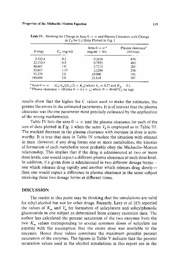
Table IV. Showing the C h a n g e in Area 0 --* oe and P l a s m a Clea rance wi th C h a n g e in Co for C,t D a t a P lo t ted in Fig. 1

Area 0 ~ oc ~ P l a s m a c learance b D (mg) Co (mg/ml) (mg/ml x hr) (ml /min)

9,333.4 0.2 0.1818 856. 23,333.5 0.5 0.7955 489. 46,667 1.0 2.7273 285. 53,667 1.15 3,5284 254. 93,334 2.0 10.000 156.

140,000 3.0 21.818 107.

" A r e a 0 ~ oc = (Co/V~)[(Co/2) + K,,] where V m = 0.22 and K m = 0.1. b P l a s m a clearance = (D/area 0 ~ oe) x ~o where D = 46.667C 0 (in mg).

results show that the higher the C values used to make the estimates, the greater the errors in the estimated parameters. It is of interest that the plasma clearance was the one parameter most precisely estimated by the application of the wrong mathematics.

Table IV lists the area 0 -~ oc and the plasma clearance for each of the sets of data plotted in Fig. 1 when the same V d is employed as in Table III. The marked decrease in the plasma clearance with increase in dose is note- worthy. It is true that data in Table IV simulate the situation with ethanol in man. However, if any drug forms one or more metabolites, the kinetics of formation of each metabolite most probably obey the Michaelis-Menten relationship. This implies that if the drug is administered at two or more dose levels, one would expect a different plasma clearance at each dose level. In addition, if a given dose is administered in two different dosage forms- - one which releases drug rapidly and another which releases drug slowly-- then one would expect a difference in plasma clearance in the same subject receiving these two dosage forms at different times.

DISCUSSION

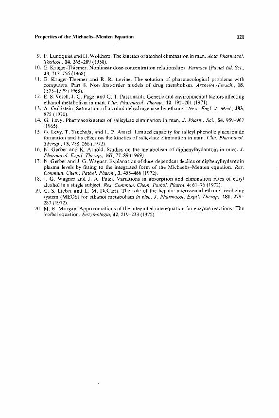
The reader at this point may be thinking that the simulations are valid for ethyl alcohol but not for other drugs. Recently, Levy et al. (15) reported the values of K,, and V,, for formation of salicylurate and salicylphenolic glucuronide in one subject as determined from urinary excretion data. The author has calculated the percent saturation of the two enzymes from the two K m values corresponding to several common doses of salicylate (as aspirin) with the assumption that the entire dose was available to the enzymes. Hence these values constitute the maximum possible percent saturation of the enzymes. The figures in Table V indicate that the percent saturation values used in the alcohol simulations in this report are in the

120 Wagner

Table V. Estimated Values of K,, and V m Reported by Levy et al. (15) and Estimated Percent Saturation of the Enzymes If the Entire Dose Were

Available to the Enzymes

Metabolite K,, (mg) V,~ (mg/hr)

Salicylurate 340 68 Salicylphenolic glucuronide 542 31

Dose of salicylate (mg)

Percent saturation of enzyme if entire dose were available to the enzyme

Salicylurate Phenolic glucuronide

300 46.9 35.6 600 63.8 52.5

1000 74.6 64.9 2000 ,~ 85.5 78.7 4000 92.2 88.1

same range as one may calculate for salicylate from the data of Levy et al.

(15). The fact that there are first-order paths parallel to the two Michaelis- Menten paths in salicylate pharmacokinetics (15) has no bearing on the calculations shown in Table V.

ACKNOWLEDGMENT

The author is grateful to Dr. Carl M. Metzler, The Upjohn Company, Kalamazoo, Michigan, for use of the program NONLIN.

REFERENCES

1. L. Michaelis and M. L. Menten. Die Kinetik der lnvertinwirkung. Biochem. Z., 49, 333-369 (1913).

2. A. F. Bartholomay. Stochastic models in medicine and biology. In Proceedings, of-a Sym- posium, Mathematics Research Center, U.S. Army, University of Wisconsin, June 12-14, (1963), pp. 105 112.

3. V. Henri. The6rie g6n~rale de Faction de quelques diastases. Compt. Rend. Hebd. S~:anc. Acad. Sci. (Paris), 135, 91(~919 (1902).

4. A. Rescigno and G. Segre. Drug and Tracer Kinetics. Blaisdell, Waltham, Mass., 1966, p. 14. 5. J. G. Wagner. A new generalized nonlinear pharmacokinetic model and its implications.

In Biopharmaceutics and Relevant Pharmacokinetics, Drug Intelligence Publications, Hamilton Press, Hamilton, Ill. (1971), pp. 302 317.

6. R. L. Dedrick and K. B. Bischoff. Pharmacokinetics in application of the artificial kidney. Chem. Engr. Prog. Svmp. Ser., 64, 32M4 (1968).

7. K. B. Bischoff and R. L. Dedrick. Thiopental pharmacokinetics. J. Pharm. Sci., 57, 1346 1357 (1968).

8. K. B. Bischoff, R. L. Dedrick, and D. S. Zaharko. Preliminary model for methotrexate pharmacokinetics. J. Pharm. Sci.. 59, 149 154 (1970).

Properties of the Michaelis-Menten Equation 121

9. F. Lundquist and H. Wolthers. The kinetics ofalcohol elimination in man. Acta Pharmacol. Toxicol., 14, 265-289 (1958).

10. E. Kriiger-Thiemer. Nonlinear dose-concentration relationships. Farmaco (Pavia) Ed. Sci., 23, 717-756 (1968).

11. E. Kriiger-Thiemer and R. R. Levine. The solution of pharmacological problems with computers. Part 8. Non first-order models of drug metabolism. Arzneim.-Forsch., 18, 1575-1579 (1968).

12. E. S. Vesell, J. G. Page, and G. T. Passonanti. Genetic and environmental factors affecting ethanol metabolism in man. Clin. Pharmacol. Therap., 12, 192-201 (1971).

13. A. Goldstein. Saturation of alcohol dehydrogenase by ethanol. New. Engl. J. Med., 283, 875 (1970).

14, G. Levy. Pharmacokinetics of salicylate elimination in man. J. Pharm. Sci., 54, 959 967 (1965).

15. G. Levy, T. Tsuchuja, and L. P. Amsel. Limited capacity for salicyl phenolic glucuronide formation and its effect on the kinetics of salicylate elimination in man. Clin. PharmacoL Therap., 13, 258 268 (1972).

16, N. Gerber and K. Arnold. Studies on the metabolism of diphenylhydantoin in mice. J. Pharmacol. Exptl. Therap., 167, 77-89 (1969).

17. N. Gerber and J. G. Wagner. Explanation of dose-dependent decline of diphenylhydantoin plasma levels by fitting to the integrated form of the Michaeli~Menten equation. Res. Commun. Chem. Pathol. Pharm., 3, 455~466 (1972).

18. J. G. Wagner and J. A. Patel. Variations in absorption and elimination rates of ethyl alcohol in a single subject. Res. Commun. Chem. Pathol. Pharm. 4:61-76 (1972).

19. C. S. Lieber and L. M. DeCarti. The role of the hepatic microsomal ethanol oxidizing system (MEOS) for ethanol metabolism in vivo. J. Pharmacol. Exptl. Therap., 181, 279- 287 (1972).

20. M. R. Morgan. Approximations of the integrated rate equation for enzyme reactions : The Veibel equation. Enzymologia, 42, 219 233 (1972).