Embed Size (px)
Citation preview

Computational Intelligence, Volume 29, Number 2, 2013
ACTION FAILURE RECOVERY VIA MODEL-BASED DIAGNOSISAND CONFORMANT PLANNING
ROBERTO MICALIZIO
University of Turin, Turin, Italy
A plan carried on in the real world may be affected by a number of unexpected events, plan threats, whichcause significant deviations between the intended behavior of the plan executor (i.e., the agent) and the observedone. These deviations are typically considered as action failures. This paper addresses the problem of recoveringfrom action failures caused by a specific class of plan threats: faults in the functionalities of the agent. The problemis approached by exploiting techniques of the Model-Based Diagnosis (MBD) for detecting failures (plan executionmonitoring) and for explaining these failures in terms of faulty functionalities (agent diagnosis). The recoveryprocess is modeled as a replanning problem aimed at fixing the faulty components identified by the agent diagnosis.However, since the diagnosis is in general ambiguous (a failure may be explained by alternative faults), the recoveryhas to deal with such an uncertainty. The paper advocates the adoption of a conformant planner, which guaranteesthat the recovery plan, if it exists, is executable no matter what the actual cause of the failure. The paper focuses ona single agent performing its own plan, however the proposed methodology takes also into account that agents aretypically situated into a multiagent scenario and that commitments between agents may exist. The repair strategy istherefore conceived to overcome the causes of a failure while assuring the commitments an agent has agreed withother team members.
Received 21 March 2011; Revised 12 December 2011; Accepted 12 February 2012; Published online 4 July2012
Key words: model-based diagnosis, plan execution monitoring, conformant planning.
1. INTRODUCTION
An agent performing a plan in the real world should be in charge of monitoring itsenvironment and the actual effects of its actions as they may fail for a number of reasons. Tomake the phase of plan execution robust to failures, many strategies to plan repair have beenrecently proposed (Gerevini and Serina 2000; van der Krogt and de Weerdt 2005a; Fox et al.2006).The basic idea of these approaches is that, during the plan execution, changes in thegoals (e.g., new goals can be added), or changes in the environment (e.g., a door expected tobe open is actually closed) make the current plan no longer adequate for achieving the desiredgoals. The plan execution is therefore stopped, and a plan repair mechanism is activated toadjust the current plan to the situation actually encountered at execution time.
As pointed out by Cushing and Kambhampati (2005), however, plan repair cannot assumethat execution failures are independent of the agent’s behavior; when such an assumption ismade, the agent might repeat indefinitely the same error. For instance, let us consider theblocks world domain and assume that an agent fails in picking a block up because of an errorin calculating the movements of its arm, in this case adapting the initial plan by introducinga new pick up action may resolve the problem. However, if the same pick up action fails dueto a fault in the agent’s arm, there will be no advantage in trying to execute that action againsince it would inevitably fail. To overcome this situation, one should first remove the rootcauses of the failure (i.e., the fault in the handling apparatus), and then attempt to repair theplan by inserting in the original plan a new pick up action.
In this paper, we intend to complement previous approaches to plan repair by takinginto account the problem of recovering from action failures caused by faults. To this end, we
Address correspondence to Roberto Micalizio, Dipartimento di Informatica, Universita di Torino, corso Svizzera 185,10149 Torino, Italy; e-mail: [email protected]
C© 2012 Wiley Periodicals, Inc.

234 COMPUTATIONAL INTELLIGENCE
adopt Model-Based Diagnosis (MBD) to detect action failures (plan execution monitoring)and to explain these failures in terms of faulty functionalities (agent diagnosis).
Our idea, in fact, is that the first step for handling effectively an action failure consistsin removing the root causes of the failure identified by the agent diagnosis, and restoring thenominal conditions in the agent functionalities. After this fundamental step, either the agentresumes the execution of the original plan from the same point where it was stopped; or, ifrequired, a plan repair mechanism is invoked to adjust the rest of the plan. In this paper, wewill focus on the problem of recovering from an action failure so that the execution of theoriginal plan can be resumed.
One of the main challenges in pursuing this objective is that the agent diagnosis cannotbe anticipated; thus the recovery strategy must be based on a planner which synthesizes on-the-fly a recovery plan, and whose goal consists in fixing the faulty functionalities mentionedby the agent diagnosis. Moreover, the agent diagnosis is typically ambiguous (several faultscan explain the same action failure), thereby the planner synthesizing the recovery plan mustbe able to deal with such ambiguity. To cope with these problems, we adopt a conformantplanner as this kind of planners is able to deal with ambiguous initial states, and assures thatthe recovery plan, when it exists, is executable even though the actual cause of the failure isnot precisely known.
Albeit the recovery strategy we propose is based on a single agent that can just changeits own plan, we also consider the problem from a wider point of view by situating the agentinto a multiagent setting. When an agent shares its environment with other agents, it has toconsider that its recovery plan may interfere with the plans the other agents are carrying on.In this paper, our objective is to make the recovery process of an agent transparent to allthe other agents. This means that, on one side the recovery cannot acquire new resourcesto avoid negotiations with other agents; on other side, the recovery must guarantee that thecommitments an agent has already agreed with other team members will be preserved. Themultiagent setting is given by a Multiagent Plan (MAP) (Durfee 2001), in which commitmentsand dependencies among agents are explicitly represented as precedence and causal linksbetween action instances.
A further difficulty in dealing with a multiagent scenario is that, when a recovery plandoes not exist (e.g., an agent cannot fix a fault on its own), the impaired agent can becomea latent menace for the other agents; for instance, an agent may lock indefinitely criticalresources. We try to limit the impact of unrecoverable faults by switching the goal of therecovery strategy from “fixing the faulty functionalities” to “reaching a safe status,” thatis, a state where the impaired agent does not hold any resource. As we will see, the mainadvantage of the proposed approach is that the conformant planner used for the synthesis ofa recovery plan can also be used for the synthesis of a plan to the safe status.
1.1. Organization
The paper is organized as follows. The next section recalls some basic notions aboutclassical planning and multiagent planning; these concepts are then exemplified in Section 3where we briefly introduce a multiagent scenario that will be used to illustrate the proposedmethodology throughout the paper. Section 4 delineates the main control strategy that allowsan agent to coordinate with other teammates and to supervise the progress of its ownlocal plan. The following three Sections, 5, 6, and 7, discuss the three activities involvedin the control strategy: the monitoring, the diagnosis and the recovery, respectively. Inparticular, the recovery relies on a conformant planner, which is presented in Section 8 wherewe also motivate why a recovery plan must satisfy a so stringent requirement. In Section 9we go back to the example and show how the control strategy actually intervenes duringthe execution of a MAP by detecting and recovering from action failures. The effectiveness

ACTION FAILURE RECOVERY: A MODEL-BASED APPROACH 235
of the repair methodology is discussed in Section 10, in which an extensive experimentalanalysis is presented. Finally, in Section 11 the proposed approach is compared with otherrelevant works in the literature.
2. BACKGROUND
In this section we briefly recall some basic notions on classical and multiagent planningwhich will be useful in the rest of the paper.
2.1. Classical Planning
Classical planning is traditionally formalized in terms of propositional logics.1 Accordingto Nebel (2000), in the propositional framework a system state s is modeled as a subset ofliterals in �, that is the set of all the propositional atoms modeling the domain at hand. Eachliteral can appear in its positive or negated form. A plan operator (i.e., an action instance)o ∈ 2� × 2� is defined by a set of preconditions pre ⊆ � and its effects eff ⊆ �; where �is the set � augmented with ⊥ (i.e., false) and � (i.e., true).
The application of an operator o to a state s is defined as App : 2� × o→ 2�
App(s, o) ={
(s −¬eff (o)) ∪ eff (o), if s |= pre(o) and s |= ⊥ and eff (o) |= ⊥{⊥}, otherwise.
Of course, actions are deterministic: when the preconditions pre(o) are satisfied in s,the effects eff (o) are always achieved.
A planning problem is the tuple � = 〈�, O, I, G〉 where:
1. � is the set of propositional atoms, also called fact or fluent;2. O ⊆ 2� × 2� is the set of available plan operators;3. I ⊆ � is the initial state;4. G ⊆ � is the goal state.
Solving a planning problem requires to find a sequence of plan operators that whenapplied to the initial state I reaches the goal state G.
2.2. Multi-Agent Planning
A MAP can be seen of as an extension of a Partial-Order Plan (POP) (Weld 1994) wheredeterministic actions, rather than being assigned to a single agent, are distributed among anumber of cooperating agents in a team T . Since agents share the same environment, theyalso share the same set of critical resources RES ; that is, resources that can only be accessedin mutual exclusion. A MAP has therefore to achieve the expected goals while guaranteeingthe consistent access to the resources. The formalism we adopt for modeling a MAP is asimplified version of the formalism presented by Cox, Durfee, and Bartold (2005). In ourview, a MAP instance P is the tuple 〈T , RE S, A, E, C, R〉, where:
1. T is the team of agents; agents will be denoted by the letters i and j ;2
2. RES is the set of critical resources available in the environment; in this paper we assumethat all the resources are renewable: they can be locked and relinquished by an agent,
1See, for instance, the seminal works about STRIPS (Fikes and Nilsson 1971), and more recently the Planning DomainDefinition Language (PDDL) (Ghallab et al. 1998; Fox and Long 2003).
2In principle, agents could be heterogeneous; that is, two agents may have different actuators; but for the sake of simplicityin the discussion, we will assume that all the agents are of the same type.

236 COMPUTATIONAL INTELLIGENCE
but are never consumed; for instance, renewable resources are tools, locations, objects,and so on;
3. A is the set of the action instances the agents have to perform. Each action instancea ∈ A is assigned to a specific agent i ∈ T ;
4. E is a set of precedence links between actions: a precedence link a ≺ a′ in E indicatesthat a′ can start only after the completion of action a;
5. C is a set of causal links of the form cl : aq→ a′; the link cl states that the action a
provides the action a′ with the service q (q is an atom occurring both in the effects of aand in the preconditions of a′);
6. R is a set of precedence links specifically used to rule the access to the resources. Theselinks have the form a ≺res a′, meaning that action a precedes a′ in the use of resourceres ∈ RES .
While causal links model the exchange of services between agents, precedence links in Rguarantee the concurrency requirement Roos and Witteveen (2009), for which two actions aand a′, assigned to different agents, cannot be executed at the same instant if they require thesame resource res; the two actions must be serialized by adding either a ≺res a′ or a′ ≺res ain R.
The goal G achieved by the MAP instance P consists of a conjunction of propositionsthat must hold in the final state. In general, an agent is responsible for providing just a subgoaland hence a subset of the propositions mentioned in G.
The problem of synthesizing the MAP P is outside the scope of this paper, possiblesolutions have been addressed in Boutilier and Brafman (2001), Jensen and Veloso (2000),and Cox et al. (2005). Independently of how the MAP P has been built, we assume it satisfiesthe following properties:
1. executable: the plan is deadlock free, and the concurrency requirement is satisfied;2. correct: all the domain-dependent constraints on the use of resources are satisfied, and the
global goal is actually reached if no unexpected event occurs during the plan execution.
2.3. Local plans
In our approach, each agent has just a partial view of the MAP P; in particular, an agenti knows just its own local plan Pi = 〈Ai , Ei , Ci , T i
in, T iout, Ri
in, Riout〉: Ai , Ei , and Ci have
the same meaning as A, E , and C , respectively, restricted to actions assigned to agent i .Thus Ei and Ci only contain links between actions in Ai . Whereas the sets T i
in, T iout, Ri
in, andRi
out contain links between actions of different agents. More precisely, T iin is a set of incom-
ing causal links of the form aq→ a′ where a′ belongs to Ai and a is assigned to another
agent j in T ; T iout is a set of outgoing causal links a
q→ a′ where a ∈ Ai and a′ ∈ A j (i = j).Similarly, Ri
in is a set of incoming precedence links of the form a ≺res a′ where a′ belongsto Ai and a is assigned to another agent j in the team; finally, Ri
out is a set of outgoingprecedence links a ≺res a′ where a ∈ Ai and a′ ∈ A j .
For the sake of simplicity, we assume that each local plan Pi extracted from P is totallyordered, and hence Pi can be seen as the ordered sequence of actions [ai
0, ai1, . . . , ai
n, ai∞].
Where, as usual in partial-order planning, ai0 and ai
∞ are two pseudo actions modeling,respectively, the initial state and the subgoal of the local plan Pi (Weld 1994).

ACTION FAILURE RECOVERY: A MODEL-BASED APPROACH 237
FIGURE 1. The set of action templates in the office domain.
3. AN EXAMPLE
Let us consider a simple applicative scenario where two agents, A1 and A2, provide adelivery service in an office. The task domain is modeled in propositional terms through thefollowing set of atoms:
1. place: denotes the resources available in the environment. In our example, we aregoing to consider an office with two desks, place(Desk1) and place(Desk2), arepository for the parcels, place(Rep), and a parking area place(Parking). Therepository and the two desks are critical resources that can be accessed by no more thanone agent at any time instant, while Parking is not constrained and hence many agentscan be simultaneously located in it;
2. position: models the position of an agent, for instance position(A1, Rep)means that the agent A1 is located within the repository;
3. at: models the position of an object, namely the parcels the agents have to deliver tothe desks; for instance at(Pack1, Rep) means that the parcel Pack1 is stored intothe repository Rep;
4. loaded: indicates whether an agent is carrying an object or not, the atomloaded(A1,Pack1) states that A1 is loaded with the parcel Pack1, whereas loaded(A1,empty) means that A1 is not carrying any object.
Figure 1 shows some examples of action templates in our office domain. The go actiontemplate models the movement of an agent from a place FROM to another place TO. Whilethe load and unload action templates describe how an agent can operate on a parcel. Ofcourse, these templates need to be instantiated with regard to concrete atoms to obtain anaction instance that an agent can actually perform.
Let us assume that, as a general rule, agent A1 is in charge of delivering parcels to deskspicking them up from the repository; while agent A2 is in charge of collecting parcels fromdesks and taking them back to the repository. In our specific case, we have that agent A1is assigned to deliver parcel Pack1 to Desk1 while agent A2 has to move the two parcelsPack1 and Pack2 back to the repository. Of course, agent A2 expects to collect parcelPack1 from Desk1, and hence agent A1 has to deliver that parcel first.
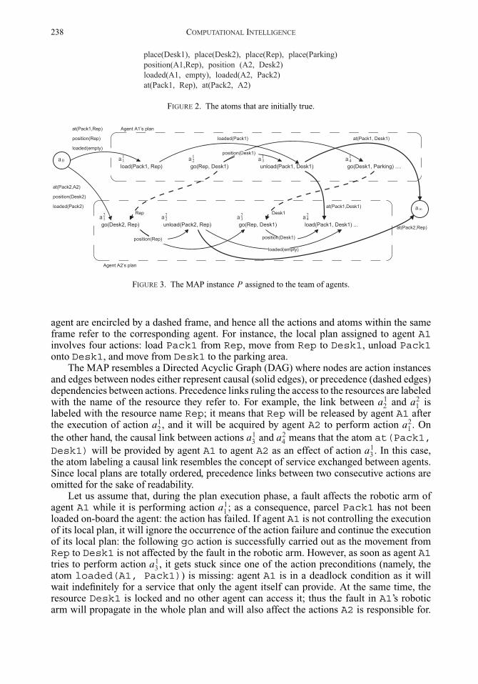
The initial set of atoms is given in Figure 2: agent A1 is in the repository and it is empty,so it is ready to load parcel Pack1; agent A1 is in Desk2 and already loaded with parcelPack2. Figure 3 shows a portion of the MAP assigned to the two agents. For the sake ofreadability of the picture, action instances and atoms have been simplified by removing theagent identifier; it can be easily determined by considering that all the actions of the same
238 COMPUTATIONAL INTELLIGENCE
place(Desk1), place(Desk2), place(Rep), place(Parking)position(A1,Rep), position (A2, Desk2)loaded(A1, empty), loaded(A2, Pack2)at(Pack1, Rep), at(Pack2, A2)
FIGURE 2. The atoms that are initially true.
load(Pack1, Rep) go(Rep, Desk1) unload(Pack1, Desk1) go(Desk1, Parking) ....
go(Desk2, Rep) unload(Pack2, Rep) go(Rep, Desk1) load(Pack1, Desk1) ...
Rep Desk1at(Pack1,Desk1)
loaded(Pack1)
position(Desk1)
position(Rep) position(Desk1)
Agent A1’s plan
Agent A2’s plan
at(Pack1, Desk1)
at(Pack1,Rep)
position(Rep)
loaded(empty)
at(Pack2,A2)
position(Desk2)
loaded(Pack2)
loaded(empty)
at(Pack2,Rep)
a0
a∞
a11 a12 a13 a14
a21 a22 a23 a24
FIGURE 3. The MAP instance P assigned to the team of agents.
agent are encircled by a dashed frame, and hence all the actions and atoms within the sameframe refer to the corresponding agent. For instance, the local plan assigned to agent A1involves four actions: load Pack1 from Rep, move from Rep to Desk1, unload Pack1onto Desk1, and move from Desk1 to the parking area.
The MAP resembles a Directed Acyclic Graph (DAG) where nodes are action instancesand edges between nodes either represent causal (solid edges), or precedence (dashed edges)dependencies between actions. Precedence links ruling the access to the resources are labeledwith the name of the resource they refer to. For example, the link between a1
2 and a21 is
labeled with the resource name Rep; it means that Rep will be released by agent A1 afterthe execution of action a1
2 , and it will be acquired by agent A2 to perform action a21 . On
the other hand, the causal link between actions a13 and a2
4 means that the atom at(Pack1,Desk1) will be provided by agent A1 to agent A2 as an effect of action a1
3 . In this case,the atom labeling a causal link resembles the concept of service exchanged between agents.Since local plans are totally ordered, precedence links between two consecutive actions areomitted for the sake of readability.
Let us assume that, during the plan execution phase, a fault affects the robotic arm ofagent A1 while it is performing action a1
1; as a consequence, parcel Pack1 has not beenloaded on-board the agent: the action has failed. If agent A1 is not controlling the executionof its local plan, it will ignore the occurrence of the action failure and continue the executionof its local plan: the following go action is successfully carried out as the movement fromRep to Desk1 is not affected by the fault in the robotic arm. However, as soon as agent A1tries to perform action a1
3 , it gets stuck since one of the action preconditions (namely, theatom loaded(A1, Pack1)) is missing: agent A1 is in a deadlock condition as it willwait indefinitely for a service that only the agent itself can provide. At the same time, theresource Desk1 is locked and no other agent can access it; thus the fault in A1’s roboticarm will propagate in the whole plan and will also affect the actions A2 is responsible for.

ACTION FAILURE RECOVERY: A MODEL-BASED APPROACH 239
Moreover, even though the system is blocked, no recovery strategy is activated as no failurehas been detected.
This simple example shows the necessity of detecting action failures as soon as possibleand properly reacting to them. The methodology we propose in this paper handles actionfailures in two ways: first, it tries to recover from a failure by fixing the faulty components;second, when the faulty components cannot be fixed, the methodology tries to reduce theimpact of the failure by moving the impaired agent into a “safe condition,” that is a conditionwhere the agent does not hold any resource and does not hinder other teammates.
4. DISTRIBUTED CONTROL STRATEGY
In a multiagent setting, where the execution of a MAP is carried on in parallel by a teamof cooperating agents, it appears natural to adopt a distributed approach also for the controlof the plan execution. This means that each team member must be able to:
1. Determine when the preconditions of the next action to perform are satisfied;2. Activate the execution of the next action;3. Determine the outcome of the last performed action;4. In case of nonnominal outcome, activate a strategy for recovering from the failure so
that the plan execution can be resumed.
To get these results, we propose a local control task consisting of three main activities:
1. plan execution monitoring, corresponding to the fault detection phase in the MBDterminology, tracks the status of the agent over time while the plan execution is inprogress, and detects deviations between the expected and the observed agent’s behavior.In this paper, such deviations can only be due to nonobservable faults affecting the agent’sfunctionalities;
2. agent diagnosis, corresponding to the fault identification phase in MBD, explains thedetected action failures in terms of faults in the agent’s functionalities;
3. action recovery aims at bringing the status of an agent back to its nominal conditions;the recovery has to fix the components that have been qualified as faulty by the agentdiagnosis. In this paper we propose a local recovery strategy which only intervenes onthe plan of the impaired agent while it is completely transparent for all the other agentsin the team.
Since agents execute their actions concurrently, they need to coordinate with one another toavoid the violation of the constraints defined during the planning phase. Effective coordina-tion is obtained by exploiting the causal and precedence links in P . As pointed out by Deckerand Li (2000), in fact, coordination between agents i and j is required when i provides j
with a service q. This is explicitly modeled in our framework by a causal link cl : aih
q→ a jk
in C , which belongs both to T iout and to T j
in as an effect of the decomposition of P . Therefore,on the one hand cl ∈ T i
out tells agent i to send agent j a message about the service q assoon as the action ai
h has been completed; on the other hand, cl ∈ T jin tells agent j that to
perform action a jk a message about the service q has to be received from agent i . Likewise,
the consistent access to the resources is a form of coordination which involves precedencelinks.

240 COMPUTATIONAL INTELLIGENCE
FIGURE 4. The local control strategy.
It follows that coordination among agents is only possible when the following require-ment is satisfied.
Requirement 1. Observability requirement. Each agent observes (at least) the directeffects of the actions it executes.
Note that this requirement must be satisfied even under the hypothesis that no fault canoccur as the plan execution is distributed and agents are not synchronized with one another.Moreover, since we are interested in monitoring the plan execution even when somethingwrong occurs, we also assume:
Assumption 1. Determinable outcome. The amount of observations an agent receivesare always sufficient to determine the outcome of every action the agent performs.
This means that right after the execution of an action, the agent is able to determinewhether the action effects have been achieved or not. Intuitively, the outcome of an actioncan be either succeeded or failed; this concept will be formalized in Section 5 together withthe process that leads an agent to the detection of action failures.
The control strategy is sketched3 in Figure 4 showing the high-level steps followed by anagent i while it is carrying on its local plan Pi . Each iteration of the while loop takes care ofthe execution of a single action: first, the agent determines its next action ai
l to be performed(line 02), then it verifies whether the action preconditions are satisfied or not (line 03). Notethat, since the plan P is correct, and since an agent immediately discovers the failure of oneof its own actions (Assumption 1), the preconditions of an action can be unsatisfied onlywhen some services that other agents have to provide are still missing. Thus, when action ai
lis not executable yet, the agent keeps waiting for the missing services.
3To keep the algorithm simple, the interagent communication has been omitted.

ACTION FAILURE RECOVERY: A MODEL-BASED APPROACH 241
On the other hand, when the action preconditions are satisfied, action ail is actually
performed in the real world (line 04).The outcome of an action is determined by the Monitoring activity (line 06) relying on
the set of observations received by the agent. When a nonnominal outcome is detected, theDiagnosis (line 10) is activated to explain such an outcome and to provide the Recoverystrategy with useful pieces of information. Recovery returns either a new local plan Pi
(overcoming the problems which caused the nonnominal outcome) or an empty plan whenthe recovery strategy failed in finding a solution. In this last case, the execution of the localplan Pi is stopped. Of course, when the local recovery fails in handling a failure, a globalplan repair strategy might be activated, such an option, however, is outside the scope of thispaper.
Note that the while loop ends with the increment of the time t (line 15), this representsjust a local clock for the agent i , namely, the agents are not temporally synchronized withone another.
In the rest of the paper we will examine these three activities (monitoring, diagnosis,and recovery), providing for each of them a formalization in terms of Relational Algebraoperators.
5. MONITORING THE EXECUTION OF A LOCAL PLAN
In this section we address the first step of the control loop previously discussed: the planexecution monitoring. As sketched in Section 4 the main objective of the monitoring taskconsists in detecting discrepancies between the expected behavior of agent i and its actual,observed activity.
To reach this objective, the monitoring needs two types of action models. The first typeis the one used during the planning phase, where just the nominal evolution of an action isrepresented in terms of preconditions and effects. These models are used by the monitoringto create expectations about the correct agent’s behavior. The second type of models is anextended version of the previous one which also includes anomalous evolutions of actions.These models describe how an agent behaves when a fault occurs during the execution of agiven action, and are used to trace the actual agent’s behavior. By comparing the expectedto the actual agent’s behavior, the monitoring task is able to detect discrepancies and henceaction failures.
In the remainder of this section we first formalize the extended action models and thenthe process that leads to the detection of action failures.
5.1. Agent Status
While the propositional language appears to be adequate during the planning phase (seeSection 2), it becomes awkward to deal with when one has to consider the plan execu-tion phase. Previous works on plan diagnosis (Roos and Witteveen 2009; de Jonge, Roos,and Witteveen 2009) have already shown that a state-based description of the world, withnon-Boolean status variables, is more effective as it is easier to update when actions areactually performed, especially when unexpected deviations may occur. In this subsection weintroduce the notion of agent status as a set of (non-Boolean) status variables; note that thisrepresentation is not in contrast with the propositional representation given above, in fact itis always possible to map each propositional atom into one (or more) status variables, andvice versa (Brenner and Nebel 2009).

242 COMPUTATIONAL INTELLIGENCE
Given an agent i ∈ T , the status of agent i is modeled by a set of discrete status variablesVARi ; for each variable v ∈ VARi , dom(v) denotes the finite domain of v . The set VARi ispartitioned into three subsets END i , ENV i , and HLT i :
1. END i maintains endogenous status variables modeling the internal state of agent i ; forinstance, in the example sketched in Section 3, endogenous variables are: position wheredom(position) = {Rep, Desk1, Desk2, Parking}, and loaded where dom(loaded)= {Pack1, Pack2, empty}; the empty value is added to model an agent which is notcarrying any parcel.
2. ENV i maintains variables concerning the environment where agent i operates, namely,the status of the available resources. Let RES be the set of available resources, for eachresource resk ∈ RES , ENV i includes a private variable resk,i whose domain is {in-use,not-in-use, unknown}: resk,i = in-use indicates that resource resk is being used by agenti at the current time; resk,i = not-in-use means that resource resk is assigned to agent ibut it is not currently used; finally, resk,i = unknown means that the agent i has no accessto resource resk . As we discuss in Section 7, the distinction between a resource in use,unused, or unknown, is essential during the recovery phase to determine the objective ofa repairing plan.
Of course, since a resource variable is duplicated in as many copies as there are agents,maintaining the consistency among all these copies could be an issue. In our approach,however, this issue does not arise since conflicts for accessing the resources are solvedat planning level. In fact, the precedence links in R guarantee that, at each time t ,a resource resk can only be used by a specific agent i ; thereby for any other agentj ∈ T \ {i} the status of the resk is unknown. In the rest of the paper we will denote asAvRes(i , t) (available resources) the subset of resources that agent i holds at time t ; thatis, AvRes(i , t) = {resk ∈ RES |resk,i = unknown}.
3. HLT i is the set of variables modeling the health status of agent i . In fact, while in manyapproaches to plan repair (see, e.g., Gerevini and Serina 2000; van der Krogt and deWeerdt 2005a) plan deviations are due to unexpected changes in the environment; in ourframework plan deviations are caused by faults in some agent’s functionalities. For thisreason, we associate each agent functionality f with a variable v f ∈ HLT i modelingthe current operative mode of f ; dom(v f ) = {ok, abn1, . . . , abnn}, where ok denotesthe nominal mode, while abn1, . . . , abnn denote anomalous or degraded modes. Forexample, the agent’s arm is modeled via the variable hnd (i.e., handling functionality)whose domain is the set {ok, blocked}; while the agent’s battery is modeled by thevariable pwr whose domain is {ok, low, flat}.
It is important to note that, while the variables in END i and in ENV i can be mapped withthe propositional formalism previously discussed, the variables in HLT i have been addedto capture the possible occurrence of faults, which is an aspect not considered during theplanning phase.
The status of agent i is therefore a complete assignment of values to the variables inVARi . It is worth noting that the status of an agent evolves over time according to the actionsit executes. Thus, an agent status is a snapshot of the agent taken at a given step of the planexecution. As we will see, the monitoring task has to consider consecutive agent states, so itis convenient to have a copy of the variables in VARi labeled with the time instant they referto. In the rest of the paper, we denote as VARi
t the copies of the status variables encodingthe status of agent i at time t .

ACTION FAILURE RECOVERY: A MODEL-BASED APPROACH 243
5.2. Extended Action Models
The main purpose of an extended action model is to describe how an action can deviatefrom its expected behavior when a subset of agent’s functionalities is not operating under thenominal mode; we propose to represent these extended action models as relations:
Definition 1. The extended model of action ail is the tuple:
〈AVAR(ail ), PRE (ai
l ), EFF (ail ), �(ai
l )〉, where:
1. AVAR(ail ) = {v1, · · · , vm} ⊆ VARi is the subset of active status variables; that is, they
are relevant for capturing all the changes which may occur in the status of agent i duringthe execution of action ai
l .2. PRE (ai
l ) ⊆ dom(v1)× · · · × dom(vm), is the set of preconditions of action ail .
3. EFF (ail ) ⊆ dom(v1)× · · · × dom(vm), is the set of effects of ai
l .4. �(ai
l ) ⊆ PRE (a il )× EFF (a i
l ) is the transition relation binding preconditions to effects.
All the passive variables in VARi/AVAR(ail ) are assumed to be persistent during the
execution of action ail .
Note that, since action ail is executed at a given time t , the transition relation �(ai
l )models the changes in the agent status from time t (when the action starts) to time t + 1(when the action ends). Hereafter ai
l (t) will denote that agent i started the execution of ail at
time t ; for readability, we will omit the time whenever it is not strictly required.Since not all the agent’s functionalities are typically required during the execution of
action ail , we highlight the subset of relevant functionalities through the following subset:
healthVar (ail ) = HLT i ∩ AVAR(ai
l )
the functionalities included in this set are essential for the successful completion of actionai
l ; in fact:
Property 1. The outcome of action ail (t) is succeeded if and only if for each variable v ∈
healthVar(ail ), v assumes the value ok at time t .
Namely, when all the functionalities healthVar(ail ) are nominal, action ai
l behaves de-terministically and its outcome is succeeded; whereas when at least one functionality is notnominal, the action behaves nondeterministically and its outcome might be failed.
5.2.1. Running example. Let us consider the go action a12 of our running example.
The template for the nominal model of such an action is given in propositional terms inFigure 1; the corresponding extended action model is sketched in Table 1 and it is representedas a relation. The active variables mentioned in the extended model are: pos (i.e., position),loaded, pwr (i.e., the power level of the battery) and engTmp (i.e., the temperature of theengine); these two last variables are health status variables, and hence there are included inhealthVar(a1
2).Each row of the extended model represents a state transition relating the active variables
at time t to the same active variables at time t + 1. The first two of them are nominal transitionas they model the expected effect of the go action when the agent is empty or is loaded,respectively. The third and fourth rows model degraded conditions; that is, even though theagent is somehow impaired, it can move from Rep to Desk1 when it is empty. However, inthe same healthy conditions, the agent cannot move when it is loaded with an object. The last

244 COMPUTATIONAL INTELLIGENCE
TABLE 1. The Extended Model of Action a12 :go(Rep,Desk1) (a Simplified Version).
Active variables at time t Active variables at time t + 1
pos loaded pwr engTmp pos loaded pwr engTmp
1 nominal Rep empty ok ok Desk1 empty ok ok2 nominal Rep obj ok ok Desk1 obj ok ok3 degraded Rep empty low ok Desk1 empty low ok4 degraded Rep empty ok hot Desk1 empty ok hot5 faulty Rep obj low ok Rep obj low ok6 faulty Rep obj ok hot Rep obj ok hot7 faulty Rep obj ok ok Rep obj low ok8 faulty Rep obj ok ok Desk1 obj low ok
four rows represent faulty transitions; in particular, rows 7 and 8 show how the same fault inthe battery (a drop from ok to low in the power level), may have nondeterministic impactson the go action: the agent cannot even leave Rep (row 7); the agent moves to Desk1 asexpected (row 8), but after this step it will not be able to move anymore.
Note that the model in the table is very partial; as we will discuss in the experimentalresults section, the action models actually used during our tests may include more than 100state transitions, and mention more than 20 active variables.
5.3. Fault Detection
5.3.1. Agent belief state. Requirement 1 guarantees that after the execution of anaction at time t , agent i receives at time t + 1 a set of observations—denoted as obsi (t +1)—that conveys pieces of information about the action’s effects. Although we assume thatobservations are correct, they are in general incomplete: an agent can just directly observethe status of its available resources, and the value of a subset of variables in END i (i.e., notall the variables in END i are observed at each time). Whereas variables in HLT i cannotbe observed and their actual value can only be inferred. As a consequence, the monitoringtask cannot be so accurate to precisely estimate the current status of agent i . In general, themonitoring is able to infer a belief state; that is, a set of alternative agent’s states which areall consistent with the received observations and hence are all possible. In the remainder ofthe paper, Bi (t) will refer to the belief of agent i inferred at time t .
5.3.2. Estimating the agent belief state. The estimation process aims at predictingthe status (i.e., the belief state) of agent i at time t + 1 after the execution of action ai
l (t); itis formalized in terms of the Relational Algebra operators as follows (see the Appendix fora short introduction about the Relational Algebra operators).
Definition 2. Let Bi (t) be the belief state of agent i , and let �(ail (t)) be the transition
relation of action ail executed at time t ; the agent belief state at time t + 1 results from:
Bi (t + 1) = PROJECTVARit+1
(SELECTobsi (t+1)(Bi (t)JOIN �(ail (t)))).

ACTION FAILURE RECOVERY: A MODEL-BASED APPROACH 245
Let us examine this expression in detail. The first step for estimating the new belief stateis the join operation between Bi (t) and �(ai
l (t)); this is the predictive step by means ofwhich all the possible agent states at time t + 1 are estimated. More precisely, each tuplein �(ai
l (t)) can be thought of as having the form 〈activeVariables t , activeVariables t+1〉,describing the transition from the active variables at time t to the active variables at time t +1. The (natural) join operator compares activeVariables t to the current belief state Bi
t , and ifBi
t � activeVariables t , the tuple is included within the join result and brings the assignmentsin activeVariables t+1 as an estimation of the next agent status. Since all the variables whichare not active are assumed persistent, the result of the join operation is a new relation havingthe form 〈VARi
t ,VARit+1〉; that is to say, a relation mapping an agent state at time t (i.e.,
belonging to Bit ) with a possible agent state at time t + 1 (built by means of the extended
action model). Of course, such a relation might contain spurious estimates; the selectionover obsi (t + 1) is therefore used to refine the result of the join operation by pruning off allthe estimates which are inconsistent with the agent’s observations. Finally, the belief stateBi (t + 1) results from the projection over the status variables of agent i at time t + 1.
Under the assumption that the action model �(ail (t)) is correct and complete the following
property holds.
Property 2. Let Bi (t) be the belief state of agent i at time t , and let s ∈ Bi (t) be theactual status of the agent i at time t ; given the extended action model �(ai
l (t)), the agentbelief state Bi (t + 1) inferred according to Definition 2 always includes the actual state s ′ ofagent i at time t + 1.
Proof . By contradiction, let us assume that the state s ′ does not belong to the belief stateBi (t + 1); this might happen for one of the following reasons:
(1) a state transition 〈s, s ′〉 is missing in �(ail (t)), but this is against the assumption of
correctness and completeness of the action model;(2) the state transition 〈s, s ′〉 is included in �(ai
l (t)), but the actual state s is not includedin Bi (t), but this is against the premises of the property;
(3) the state s ′ is correctly estimated via the join operator, but it is filtered out during theselection which prunes off all the agent states inconsistent with the observations. Butthis is against the assumption that the available observations, though incomplete, arecorrect. �
Property 2 assures that the monitoring is correct as the actual status of an agent is alwaystraced during the plan execution.
5.3.3. Inference of an action outcome. To infer the outcome of an action we adopt aconservative approach asserting that an action has outcome succeeded when the followingcondition holds:
Definition 3. Given the belief Bi (t + 1), the outcome of action ail (t) is succeeded if
and only if ∀s ∈ Bi (t + 1), s � eff (a il ). This condition states that action ai
l is success-fully completed when the nominal effects of the action hold in every state s belong-ing to the belief state inferred just after the execution of the action. This means thatwe adopt a rather pessimistic approach, in fact it is sufficient that the action effects

246 COMPUTATIONAL INTELLIGENCE
FIGURE 5. The Monitoring task.
TABLE 2. The Agent Belief State at the Time of the Failure of Action a12 .
pos loaded pwr engTmp hnd
i1 Rep Pack1 ok high oki2 Rep Pack1 low ok ok
are not satisfied in just one state in Bi (t + 1) to conclude that action ail (t) has outcome
failed.4
5.3.4. The Monitoring Task. After these premises, the monitoring task is summarizedin the pseudo-code of Figure 5. The first step consists in the estimation of the next belief stateBi (t + 1) according to Definition 2 (line 00). To determine whether the action outcome issucceeded or not, we build a temporary relation T emp as the join between Bi (t + 1) and thenominal action effects eff (a i
l ) (line 01); T emp will keep the same states as Bi (t + 1) onlyif the nominal effects of ai
l are satisfied in every state of Bi (t + 1); therefore, when T empis a proper subset of Bi (t + 1) we can conclude that the action outcome is failed (line 02);otherwise, the action outcome is succeeded (line 03).
See the Appendix for an analysis of the computational complexity of the monitoring taskimplemented by means of the Ordered Binary Decision Diagrams (OBDDs).
5.3.5. Running example. Let us assume that agent A1 has successfully completedaction a1
1 , so it is now located into the repository Rep and loaded with Pack1. The agentthen executes the subsequent go action to move from Rep to Desk1. To monitor this action,the agent exploits the model in Table 1, where the entries 2 and 5 through 8 play an activerole in estimating the possible next status of the agent. After the execution of the go action,the agent observes its current position and discovers that it is located in Rep (pos = Rep),this observation is used to refine its belief state and the result is showed in Table 2. It is easyto see that such a belief models an erroneous situation as the nominal expected effect ofaction a1
2 is pos = Desk1, which is not satisfied in any state included into the belief. Thusthe agent concludes that the go action has failed.
6. AGENT DIAGNOSIS
In this section we describe the model-based approach adopted for diagnosing action fail-ures; before that, however, we recall some basic definition about MBD. Intuitively, MBD can
4Definition 3 can be relaxed along the line discussed in Micalizio and Torasso (2008): whenever it is not possible tocertainly assert the successful or unsuccessful completion of an action, the action outcome remains pending; observationsreceived in the future will be used for discriminating between succeeded and failed.

ACTION FAILURE RECOVERY: A MODEL-BASED APPROACH 247
be viewed as an interpretation process that, given a model of the system under considerationand a set of observations about the system behavior, provides an indication of the presenceor absence of faults in the components of the system itself.
One of the first formal (logic-based) theories of diagnosis is the consistency-based diag-nosis proposed by Reiter (1987). In a consistency-based setting, the system to be diagnosedis described as a triple 〈SD,COMPS ,O〉 where:
1. SD (system description) denotes a finite set of formulae in first-order predicate logic,specifying only the system normal structure and behavior;
2. COMPS (components) is the set of system components; each component c ∈ COMPScan be qualified as either behaving abnormally ab(c), or nominally ¬ab(c);
3. O BS is a finite set of logic formulae denoting the observations.
We have a diagnostic problem when the hypothesis that all the components in COMPSbehave nominally (HNOM =
⋃c∈COMPS {¬ab(c)}) is inconsistent with the system descrip-
tion and the available observations. In other words, when SD ∪OBS ∪ HNOM |= ⊥ wehave detected an anomalous behavior of the system. Solving a diagnostic task requires tofind a subset D ⊆ COMPS of components that, when qualified as abnormal, make the newhypothesis H = {ab(c)|c ∈ D} ∪ {¬ab(c)|c ∈ COMPS \ D} consistent with the system de-scription and the observations: SD ∪ H ∪ O BS |= ⊥. The subset D is therefore a diagnosissince it identifies a subset of components whose anomalous behavior is consistent with theobservations.
Console and Torasso (Console, Theseider, and Torasso 1991; Console and Torasso 1991)have introduced the notion of abductive diagnosis by including within the system descriptionnot only the nominal states of the system but also its abnormal states and the correspondingabnormal observations. Having such a kind of system description, the diagnostic inferenceaims at finding a subset of components D such that:
(1) SD ∪ H |= O BS and(2) SD ∪ H is consistent.
Where H is again the hypothesis {ab(c)|c ∈ D} ∪ {¬ab(c)|c ∈ COMPS \ D}. This meansthat in the abductive diagnosis we are interested in identifying a subset of componentswhose anomalous behavior is not only consistent with the observations, but explains them.Moreover, having explicit fault models of the system components, it is also possible toidentify the specific abnormal behaviors affecting the impaired components.
6.1. Diagnosing Action Failures
We show now how our framework matches to the MBD concepts previously introduced.Since we are interested in detecting and diagnosing action failures as soon as they occur, themodel of an action corresponds to a portion of the system description to be used during thediagnostic inferences. Moreover, since we aim at recovering from action failures by fixingfaults, we are interested in an action model which allows us to infer an abductive diagnosis:we do not want just to know which components (i.e., agent’s functionalities) are faulty, butalso in which way.
The extended action model introduced in the previous section satisfies this requirement.In particular, Property 1 states that the outcome of an action is succeeded if and only if allthe functionalities in healthVar behave nominally; otherwise, the action fails. This means

248 COMPUTATIONAL INTELLIGENCE
that the agent diagnosis must explain the failure of an action by singling out a functionality(or a set of functionalities) which cannot be assumed to be nominal.
More formally, in our framework a diagnostic problem is the tuple
〈�(ail (t)), healthVar (ai
l ),Bi (t), obs i (t + 1)〉where:
1. �(ail (t)) is that portion of system description relevant for the diagnosis of action ai
l ,2. healthVar (ai
l ) is the set of agent’s functionalities which can be qualified as faulty,3. Bi (t) represents a piece of contextual information about the current status of agent i ,4. obsi (t + 1) is the set of available observations.
Solving such a diagnostic problem means finding a hypothesis Hi (t + 1) (i.e., an assign-ment of values to the variables in healthVar(ai
l ) at time t + 1), such that
Bi (t)∼∪ �(ai
l (t))∼∪ Hi (t + 1) � obsi (t + 1), (1)
where the symbol∼∪ means combined with. The agent diagnosis is obviously a subset Di of
variables in healthVar(ail ) such that
Hi (t + 1) = {v ∈ Di |v = ok} ∪ {v ∈ healthVar (ail ) \ Di |v = ok}
Namely, Di singles out a subset of functionalities which might have behaved erroneouslyduring the execution of action ai
l .Since we are dealing with relations, symbol
∼∪ in expression (1) corresponds to a joinoperator between relations; moreover, the entailment (�) can be matched to the select operatorof the Relational Algebra; expression (1) thus becomes:
SELECTIONobsi (t+1)(Bi (t)JOIN �(ail (t))JOIN Hi (t + 1)) (2)
that we have already met, though in a slightly different form, in Definition 2 where wehave described the process for estimating the next belief state Bi (t + 1). This means that forinferring the agent diagnosis we have just to extract the hypothesis Hi (t + 1) fromBi (t + 1):
Definition 4. Let ail (t) be an action whose outcome failed is detected within the belief
state Bi (t + 1), the qualification hypothesis explaining such a failure is
Hi (t + 1) = PROJECThealthVar (ail )Bi (t + 1)
In principle, Hi (t + 1) is a set of assignments to health status variables. Thus each tupleof this relation is a possible explanation for the failure of ai
l . In this work, however, we areinterested in singling out which functionalities can be qualified as abnormal, so the agentdiagnosis is defined as Di = {v ∈ healthVar (ai
l )|v = ok in Hi (t + 1)}
Property 3. The agent diagnosis Di inferred according to Definition 4 is correct as italways includes the actual explanation for the action failure.
Proof . The proof directly follows from Property 2, which guarantees that the actualstate s ′ of agent i at time t + 1 is included in Bi (t + 1). Since the agent diagnosis is inferredby projecting the belief status Bi (t + 1) over the health status variables of agent i , it followsthat Di includes, among others, the actual (anomalous) health status of agent i . �

ACTION FAILURE RECOVERY: A MODEL-BASED APPROACH 249
FIGURE 6. The plan repair strategy.
6.2. Running Example
Given the failure of thego action a12, agentA1 infers a qualification hypothesis by project-
ing the belief state in Table 2 over the variables in healthVar(go), namely, the variables pwrand engTmp. Consequently, the ambiguous agent diagnosis is the disjunction DA1 = {pwr=low ∨ engTmp = hot}; according to the extended action model in Table 1, in fact, it issufficient that either the battery (pwr) or the engine (engTmp) is in an anomalous mode, toprevent the agent from moving when it is loaded with an object.
7. RECOVERING FROM ACTION FAILURES: THE MAIN STRATEGY
In this section, we introduce the strategy we propose for recovering from an actionfailure. The basic idea of this strategy, sketched in Figure 6, is that the agent first tries toself-repair its impaired functionalities, and then it resumes the plan execution from the sameaction where it was stopped. Of course, the recovery builds up the results of the monitoringand diagnosis activities, so it takes in input the failed action ai
l , the last inferred belief stateBi (t + 1), and the corresponding agent diagnosis; the output consists of a recovery plan thatbrings agent i from its erroneous current situation back to a nominal condition; when therecovery plan does not exist, an empty plan is returned.
The strategy starts by determining the “healthy” agent state H, which represents thedesired situation where all the functionalities assumed to be faulty by the agent diagnosishave been fixed (line 00). Thus, in line 01, the recovered state R is synthesized as theconjunction of H and the nominal preconditions of the failed action ai
l ; R represents thesituation from which the plan execution can be resumed by trying again action ai
l . Thesubsequent step consists in the synthesis of a plan Pri reaching the state R. When Pri
exists, the plan repair strategy returns a recovery plan consisting of two parts: first theplan segment Pri which fixes the faulty functionalities, and then the original plan segment[ai
l , . . . , ai∞] (line 04).
On the other hand, when it is not possible to repair all the malfunctioning functionalities,the agent cannot complete the plan segment [ai
l , . . . , ai∞] which is aborted. In this case, the
strategy tries to take agent i into a safe status S; that is, a situation where the agent doesnot represent an obstacle for the other teammates. Therefore, even though agent i cannotcompletely recover from its failure, it can try to limit the impact of its failure in the wholesystem. If a plan Psi to the safe status exists, Psi is returned to the control loop which is incharge of executing it (lines 06-09).

250 COMPUTATIONAL INTELLIGENCE
Finally, when also the plan to safe status does not exist, the repair strategy returns anempty plan; in this case the agent interrupts the execution of its local plan.
In the rest of this section, we formalize the two planning problems that have to be solvedto achieve either the repaired status R or the safe status S. Next section will go into detailsof the conformant planner used to solve these planning problems, and explain why we needsuch a kind of planner.
7.1. Plan to RThe repaired status R is the conjunction of three conditions:
(1) all the functionalities mentioned into Di have been fixed;(2) the preconditions of action ai
l are satisfied;(3) for any action in the segment [ai
l+1, . . . , ai∞], no open preconditions are left.
The first condition removes the causes of the failure of ail , while the second and the third
ones assure that the plan segment [ail , . . . , ai
∞] is executable.A plan Pri reaching R is called recovery plan, and can be found by resolving the
following planning problem:
Definition 5. The plan Pri = [ar i0, . . . , ar i
∞] achieving R is a solution of the planningproblem 〈I,F,A〉; where:
1. I (initial state) corresponds to the agent belief state Bi (t + 1) inferred at the time of thefailure of action ai
l (t);2. F (final state) coincides with R = (
∧∀v∈Di v = ok) ∧ pre(ai
l ) ∧ grantedServices(l );3. A = is the set of action models which can be used during the planning process.
Where grantedServices(l ) = {q|q ∈ eff (ak), k < l, q ∈ pre(ah), h > l} are all those ser-vices achieved by actions preceding ai
l and consumed by actions following ail ; these services
must be included in R to avoid they are removed by some collateral effects of the recoveryplan.
Note that A contains all the actions the agent can perform, including actions whichrestore the nominal behavioral mode in the agent’s functionality. For example, a low chargein the battery (pwr = low) is fixed by means of a recharge action whose effect is pwr =ok; similarly, a high temperature in the engine (engTmp = hot) is mitigated by a refill ofa coolant fluid whose effect is engTmp = ok. In principle, these repairing actions could alsobe part of the original plan; for instance, a recharge action could be planned after a numberof actions to prevent the agent runs out of power. It is important to note, however, that somefaults cannot be autonomously repaired by the agent; for example, there is no repair actionthat can fix a blocked arm (hnd = blocked); these faults can be repaired only by humanintervention.
As mentioned earlier, when the plan Pri = [ar i0, . . . , ar i
∞] exists, the agent i yieldsits new local plan P∗i = [ar i
0, . . . , ar i∞]◦ [ai
l , . . . , ai∞]; where ◦ denotes the concatenation
between two plans (i.e., the second plan can be executed just after the last action of the firstplan has been completed).
Property 4. The plan P∗i is correct and executable.

ACTION FAILURE RECOVERY: A MODEL-BASED APPROACH 251
Proof . Both plan segments [ar i0, . . . , ar i
∞] and [ail , . . . , ai
∞] are correct and executableon their own as each of them has been produced by a specific planning step. More-over, by construction, ar i
∞ corresponds to a state where both the preconditions of ail
and the grantedServices(l ) are satisfied. It follows that the whole plan P∗i is correct andexecutable. �
7.2. Plan to SThe plan Pri may not exist as agent i could be unable to autonomously repair its faults.
The impaired agent, however, should not be left in the environment as it could become alatent menace for the other team members; for instance, the agent could lock indefinitelycritical resources preventing others from acquiring them. For this reason, the repair strategytries to move agent i into a safe status S in which i releases all its resources. Also this stepis modeled as a planning problem:
Definition 6. The plan Psi = [asi0, . . . , asi
∞] achieving S is a solution of the planproblem 〈I,F,A〉; where:
1. I (initial state) corresponds to the agent belief state Bi (t + 1) (as in the previous case);2. F (final state) is the safe status S =∧
∀resk∈AvRes(i ,t) resk,i = not-in-use;3. A is the set of action models which can be used during the planning process.
Since it is the result of a single planning phase, if the plan Psi exists, then it is alsofeasible and executable. When plan Psi exists, it becomes the new local plan assigned toagent i ; that is P∗i = Psi , and all the actions in the segment [ai
l , . . . , ai∞] are aborted.
8. A CONFORMANT PLANNER
The recovery strategy introduced in the previous section strongly relies on a plannerto either synthesize Pri or Psi ; the recovery strategy, however, must satisfy the followingdemanding requirements.
Requirement 2. Locality. The recovery strategy can only impose local changes in Pi :no new resources can be acquired for achieving either R or S.
The acquisition of a new resource would require an explicit synchronization with otheragents and hence the impact of the recovery strategy would affect, besides Pi , also the localplans of some other agents. This first requirement imposes that the planner can just exploitthe resources Av Res(i, t), already acquired by agent i at the time of the failure.
Requirement 3. Conformant Plan. Since the belief state Bi (t + 1) is in general ambigu-ous (the actual health status of the agent is not precisely known), the planning phase mustproduce a conformant plan.
This requirement assures that when the repairing plan Pri exists, it is also executable,namely, the agent can carry out that plan without the risk of getting stuck during the executionof the recovery plan.
In the remainder of the section, we will show how these two requirements shape theplanner used for the recovery purpose.

252 COMPUTATIONAL INTELLIGENCE
TABLE 3. The Model of Action a12 :go(Rep,Desk1) Refined for the Repair Purpose.
Active variables at time t Active variables at time t + 1
pos loaded pwr engTmp pos loaded pwr engTmp
1 nominal Rep empty ok ok Desk1 empty ok ok2 nominal Rep obj ok ok Desk1 obj ok ok3 degraded Rep empty low ok Desk1 empty low ok4 degraded Rep empty ok hot Desk1 empty ok hot
8.1. Refining Action Models
To integrate the planning phase within the control loop previously introduced, we presenta conformant planning algorithm based on the same Relational language we have so far usedto formalize the monitoring and the diagnostic tasks. In other words, we want to use the sameaction models envisaged for the monitoring purpose. These models, however, are too rich forthe planning purpose: an extended action model �(a) describes all the evolutions of actiona taking into account the possible occurrence of faults during its execution. From the repairpoint of view, however, it is sufficient to restrict the action model �(a) to those transitionswhich are consistent either with the agent diagnosis Di or with the nominal health status ofthe agent. In fact, on the one hand action a could be performed under the unhealthy statusassumed by Di . On the other hand, the same action could be performed when the faultyfunctionalities have been fixed and the nominal status has been restored.
Given an extended action model �(a), the corresponding refined model �(a) restrictedby the agent diagnosis Di is:
Definition 7.
�(a) ={{�(a) JOIN pre(a)} ∪ {�(a) JOIN Di } if {�(a) JOIN Di } = ∅∅ otherwise
�(a) is a subset of �(a) and it is defined only when action a can be performed given theagent diagnosis Di , in such a case it includes all the state transitions which are either nominalor consistent with Di . Otherwise, the refined model is empty.
An example of refined action model is given in Table 3 and refines the model of the goaction previously sketched in Table 1; it is easy to see that the refined model only containsthe nominal state transitions and the degraded state transitions which are consistent with theagent diagnosis DA1 = {pwr = low ∨ engTmp = high}.
8.2. Conformant Planning: Preliminaries
The conformant planning algorithm we propose is based on the same predictive mech-anism we have already used during the monitoring phase, and hence on the notion of agentbelief state. In the following discussion, however, we consider the synthesis of a plan ratherthan the plan execution; thus, when we mention an agent belief state, we will not intend astatus estimation made after the actual execution of an action, but an estimation made afterthe application (i.e., execution hypothesis) of an action to a given state.
After this premise, we define a conformant action as follows:

ACTION FAILURE RECOVERY: A MODEL-BASED APPROACH 253
Definition 8. An action a is conformant with regard to an agent belief state B if its(refined) model �(a) is applicable in every state s ∈ I.
Applying an action a to an agent belief B yields the relation:
P = B JOIN �(a) (3)
P is a set of state transitions of the form 〈s, s ′〉where s and s ′ are agent states before and afterthe application of a, respectively. The action a is conformant when each state s ∈ B matcheswith at least a transition in �(a). Of course, when P is empty, action a is not applicablein B. In all the intermediate conditions, where P is not empty but some states in B do notparticipate to the join, the action is applicable but it is not conformant.
Definition 9. Given a plan candidate π = a0, . . . , ah , and an initial agent be-lief state I = B0, the application of π to B0 is the relation Ph+1 = (((B0 JOIN �(a0))JOIN �(a1)) . . .) JOIN �(ah)
Ph+1 is a set of trajectories, each of which has the form 〈s0, s1, . . . , sh+1〉 where, exceptfor s0 which is an agent state in B0, each agent state sk+1 (k : 0..h) results by applying actionak to state sk .
The result of π is the agent belief state after the application of π to B0:
Bh+1 = PROJECTh+1Ph+15
For short, we will denote as π (B0) the agent belief state obtained by applying π to B0.In the previous section we have said that the repair strategy has to solve the planning
problem 〈I,F,A〉, where the initial state I coincides with the agent belief Bi (t + 1) uponwhich the failure of action ai
l has been detected; the final state F is either R or S; and A isthe set of action models to be used.
Definition 10. The plan candidate π = a0, . . . , ah is a conformant solution for theplanning problem 〈I,F,A〉 if:
1. π (I) � F ; that is, the goal F is satisfied in each state s ∈ π (I),and
2. a0, . . . , ah are all conformant action instances; that is, each action ak is conformant withregard to the (intermediate) agent belief state Bk extracted from Pk (k : 0..h).
To verify whether an intermediate action ak is conformant, it is sufficient to assess thefollowing property.
Property 5. ak is conformant if Bk ∩ Bextk = ∅.
Where Bk = PROJECTkPk , and Bextk = PROJECTkPk+1; namely, Bext
k is the agent beliefstate at the kth plan step (as Bk), but extracted from Pk+1; that is, after the application ofaction ak .
5To simplify the notation, the predicate h+ 1 of the project operator stands for VARih+1; that is, the agent status variables
at the (h + 1)th step.

254 COMPUTATIONAL INTELLIGENCE
Proof . By definition, action ak is conformant iff it is applicable in every state s ∈ Bk .If ak is not conformant, there must exist at least one state s ∈ Bk where ak is not applicable;as a consequence when the corresponding model �(ak) is joined with Bk , the state s doesnot participate to build the relation Pk+1. Namely, the state s is missing in Bext
k . This means
that s belongs to the dual set Bextk , and hence when ak is not conformant, Bk ∩ Bext
k cannotbe empty.
Now, let us assume that Bk ∩ Bextk = ∅ holds and conclude that ak must be conformant.
The intersection between Bk and Bextk can be empty only when Bk equals Bext
k ; this meansthat the application of the refined model �(ak) to Bk preserved in Pk+1 each state s ∈Bk . It follows that �(ak) has been applied in each state included in Bk , and hence ak isconformant. �
8.3. Search for a Conformant Solution
The conformant planning algorithm we propose adopts a forward-chaining approach thatfrom the initial state I finds a plan reaching the goal state F . More precisely, the algorithmrealizes a breadth-first strategy which carries on all the plan candidates built at a given step.
To formalize this strategy we introduce the macro-operator �, defined as follows:
Definition 11. � =⋃a∈A{�(a) such that a is executable given the resources in
AvRes(i , t)}.In other words, � is a set of refined models which just includes the actions that agent i
can perform by exploiting the resources it already holds.Our basic idea is to use � for pruning the space of plan candidates; in fact, the following
property holds.
Property 6. Given a planning problem � : 〈I,F,A〉, any conformant solution π for �that satisfies the locality requirement can only consist of actions in �.
Proof . By definition we have that: (1) � includes refined action models which areconsistent with the agent diagnosis, and this is a prerequisite for an action to be conformant;(2) � includes only the actions that are executable given the set of resources the agent alreadyholds.
Let us assume that there exists a conformant plan π including at least one action a whosemodel is not in �. If π is conformant, action a must be executable given the agent diagnosisDi (i.e., �(a) = ∅), and hence it has not been included into � as it uses resources outsideAvRes(i , t), it follows that π does not satisfies the locality requirement. On the other hand,if a just exploits resources in AvRes(i , t), a has been discarded from � as its refined model�(a) is empty, but this implies that π is not conformant against the initial hypothesis. �
Relying on the previous property, and since I equals the initial belief state B0, we cangeneralize expression (3) as follows:
PSET1 = B0 JOIN �. (4)
PSET1 is a set of P relations, and represents the set of all the plan candidates consistingof one single action. (Of course, only those actions which are applicable in B0 are actuallypart of the set PSET0.) We can further generalize expression (4) to model the space of the

ACTION FAILURE RECOVERY: A MODEL-BASED APPROACH 255
FIGURE 7. The high-level algorithm for the synthesis of a conformant plan.
(conformant) plan candidates incrementally built by applying � in succession:
PSETh+1 = PSETh JOIN � (5)
PSETh+1 is the result of h + 1 successive applications of �; it maintains all the plancandidates built by extending one step longer the previous set of candidates PSETh .
Intuitively, our planning algorithm first extends the space of the plan candidates byapplying �, and then it verifies whether there exists a plan π ∈ PSETh+1 representing aconformant solution for the problem at hand (Definition 10). Of course, since the algorithmgoes forward, we need a constant MAXDEPTH which limits the depth of the search, andguarantees the termination of the algorithm. In other words, MAXDEPTH represents themaximum number of times that it is possible to apply �. If a solution is not found in lessthan MAXDEPTH steps, the plan search terminates with a failure.
The high-level planning algorithm is showed in Figure 7; in the first five lines, someimportant structures are initialized: � is set by invoking the Build-� function which operatesaccording to equation (11); the sought plan π is empty; PSET0 (the initial explored space)just includes the initial state I; h, set to zero, counts the number of times � has been applied;finally, solved is a Boolean flag set to false; if a conformant plan is found, this flag willbe set to true, and the search will be stopped. After these preliminary steps, the algorithmloops until either a conformant solution has been found, or the number of iterations becomesgreater than MAXDEPTH .
At each iteration, the algorithm builds a new set of plan candidates PSETh+1 by ap-plying � to the previous set PSETh (line 06); PSETh+1 is therefore refined by pruningoff all those plan candidates which are not conformant, function PruneNotConformantrelies on Property 5 to achieve this objective (line 07). Note that, after the invocation offunction PruneNotConformant, PSETh+1 could become empty, this may happen when noconformant action exists, in that case the search is stopped and an empty plan is returned(line 08).
When the space of plan candidates is not empty, function CheckGoal checks whether atleast one candidate π leads to the goal F ; more precisely, π leads to a state Bh+1 where thecondition Bh+1 � F is satisfied. If this is the case, the conformant plan π is extracted fromPSETh+1, and the flag solved is turned to true (lines 09-11). Otherwise, h is incrementedand the loop is repeated.

256 COMPUTATIONAL INTELLIGENCE
If a solution has not been found after MAXDEPTH iterations, the loop is stopped andan empty plan is returned.
Note that, since the search proceeds in a breadth-first manner and keeps all the plancandidates found at a given iteration, there is no need to backtrack. Of course, an efficientimplementation of the algorithm becomes a critical issue; since the sizes of the relations mightbe very huge, the operations between relations might become computationally expensive.A possible way to mitigate the problem consists in the adoption of symbolic formalismsfor encoding the relations in a compact form. The work by Darwiche and Marquis (2002)describes and compares with one another different methodologies for compiling knowledgeinto symbolic representations. Relying on the results presented by Darwiche and Marquis, wehave adopted in our implementation the formalism of the OBDDs. The computational costof the algorithm implemented by means of OBDD operators is discussed from an empiricalpoint of view in Section 10; for a theoretical analysis of its computational complexity, seethe Appendix.
Theorem 1. Let h be the depth of the search space; when h < MAXDEPTH , theconformant planning algorithm is correct and complete.
Proof . In this proof we demonstrate that:
1. if it exists a plan π , having h steps, such that π (I) � F , then:
(i) π is a solution,(ii) π belongs to PSETh ,
(iii) the algorithm finds it;
2. otherwise, if PSETh becomes empty, then no conformant solution exists (even with anumber of steps greater than MAXDEPTH ).
With Property 6 we have already shown that any conformant plan satisfying the localityrequirement, if it exists, is a sequence of action instances in �. Since � is finite and hlimited by MAXDEPTH , the space of plan candidates is finite too. We demonstrate thatthe planning algorithm carries on an exhaustive search within this space and that it does notmiss solutions. We show this by induction:
Hypothesis: After h iterations PSETh maintains all the conformant plans satisfying thelocality requirement, each of these plan candidates has h actions.
Base Case: for h = 1 we have that PSET1, built as PSET0 JOIN �, maintains all theconformant plan candidates satisfying the locality requirement consisting of just one action.Since PSET0 equals I, the basic case is trivially satisfied (see equation 4).
Inductive step: We show that, at the (h + 1)th iteration, the synthesis of PSETh+1 doesnot lose solutions and keeps all the possible conformant plans:
(1) PSETh+1 = PSETh JOIN �:
(i) for each plan candidate π ∈ PSETh , the algorithm builds a set of new plan candidates
X [π ] :⋃a∈�{π ′| π ′ = π ◦ 〈a〉}

ACTION FAILURE RECOVERY: A MODEL-BASED APPROACH 257
Namely, for each action a ∈ �, the algorithm gets a new plan candidate π ′ byappending a in π ;
(ii) PSETh+1 is the union of the sets of plan candidates X [π ] for each π ∈ PSETh .
PSETh+1 =⋃
π∈PSETh
X [π ]
Since a plan candidate with h + 1 steps can only be obtained by appending an actionto a plan candidate with h steps, and since PSETh maintains all the (conformant)plan candidates of length h (for the inductive hypothesis), PSETh+1 contains allthe possible plan candidates having h + 1 steps, though some of them may not beconformant.
(2) The PruneNotConformant function prunes off from the PSETh+1 previously com-puted all the plan candidates π ′ which are not conformant; so after this step:
PSETh+1 = {π ′ = π ◦ 〈a〉|π ∈ PSETh and a is conformant with regard to π (I)}.Of course, PSETh+1 becomes empty when no plan π ∈ PSETh can be extended withany conformant action, and hence no plan candidates with h + 1 steps can be built.Otherwise, when PSETh+1 is not empty, it maintains all and only the conformant plansof length h + 1 obtained by appending an action to a plan π ∈ PSETh .
(3) Finally, the algorithm looks for a plan reaching the goal; function CheckGoal returnstrue when there exists a plan π ∈ PSETh+1 such that π (I) = F .
We have therefore demonstrated that the algorithm performs an exhaustive search andthat no solution is lost: for h < MAXDEPTH , the algorithm is correct and complete. �
The algorithm is not complete in general; when it terminates for h >= MAXDEPTH ,we can only assert that a solution with fewer than MAXDEPTH actions does not exist, butwe cannot state whether solutions involving a greater number of actions exist or not.
Corollary 1. When the algorithm terminates with success, the extracted solution π isoptimal in terms of number of applied actions. In other words, no conformant plan reachingthe goal with less actions than π exists; this is a direct consequence of the breadth-first searchthe algorithm carries on.
Corollary 2. When the algorithm terminates with success, PSETh+1 maintains all thepossible optimal solutions with exactly h + 1 actions.
In fact, the search carries on all the possible plan candidates found at a given step ofthe search. So far we have not exploited this property as our current implementation returnsthe first conformant solution that has been found. In general, however, one could consider toreturn the best plan with regard to some preference criteria.
8.4. Advantages and Limits of a Conformant Planner
Since the recovery strategy has to deal with ambiguous agent diagnoses, it has to exploita planner which is able to deal with belief states and nondeterministic actions. To cope withthis issue, in this paper we have proposed the adoption of a conformant planner, but thereare other kinds of planners that can deal with ambiguity as well. For instance, contingentplanning (Peot and Smith 1992) is the problem of finding conditional plans given incomplete

258 COMPUTATIONAL INTELLIGENCE
knowledge about the initial world and uncertain action effects. The basic idea of conformantplanning is to anticipate, at planning time, all the possible contingencies that may ariseduring the plan execution phase; for each contingency a contingent plan is inferred; sensingactions are thus used to identify the contingencies at execution time. Thereby, a contingentplan is not a linear plan, as in the conformant case, but it similar to a tree where theagent’s actions are interleaved with sensing actions. Contingent planning, however, doesnot seem to fit adequately the needs of the recovery strategy we have discussed. First ofall, it is not easy in our scenario to anticipate all the possible contingencies. In fact, eventhough the set of possible faults is finite, the same fault occurring in different contexts mayhave different consequences.6 Thus, predicting all the possible combinations of faults andcontextual conditions in which those faults can occur may become unpractical. Moreover,contingent planning explicitly requires that at execution time the sensing actions can observethe happening of contingencies; that is, faults, which are typically not observable.
The choice of a conformant planner is therefore motivated not only by the need to dealwith ambiguity, but also by the partial agent observability. Conformant planning, however,has also some drawbacks; first of all, it is computationally expensive (see the Appendix);in addition to that, the conformant requirement imposes a very stringent constraint on thepossible solutions, and it is easy to miss a recovery plan. The conformant planner, in fact,tries to fix all the faults assumed by the agent diagnosis; therefore, it is sufficient that one ofthem is nonrecoverable to conclude that no recovery plan exists, even though the actual faultis recoverable.
A possible way to mitigate this problem could be to consider preferred diagnoses ratherthan all the plausible diagnoses. One could synthesize a recovery plan just taking into accountthe most probable fault, and in that case a conformant planner would not even be required.Of course, the solution obtained in this way would not have any guarantee neither about itsexecutability nor about its effectiveness in restoring the nominal conditions: although a faultis more probable than others, it may not be the actual fault. Another possible solution couldbe the adoption of active diagnosis techniques to better identify the actual fault. In activediagnosis, the agent is required to perform tests intended to confirm or disconfirm a fault.We leave this aspect of the recovery problem for future research.
9. RUNNING EXAMPLE
In this section, we show how to recover from the failure of action a12 that has been
diagnosed as DA1 = {pwr = low ∨ engTmp = hot}. First of all, we determine the recoveredstate R to be reached. As discussed earlier, R must represent an agent state where the faultyfunctionalities mentioned in the agent diagnosis have been fixed, and the preconditions ofa1
2 are satisfied (the agent is ready to resume the execution of the original plan). It is easy tosee that the recovered state R coincides with the variable assignments: (pos = Rep; loaded= Pack1; pwr = ok; engT mp = ok); namely, the agent is positioned in Rep, loaded withPack1, and both the functionalities pwr and engTmp are in their nominal mode ok.
After this step, the relation � is built by considering the set of resources currentlyavailable to the agent, namely: {Rep, Desk1, Pack1, Parking}; agent A1 has the exclu-sive access to the first three resources, while the last one is a nonconstrained resource, andhence it is always available to any agent. It follows that � = {go(A1,Rep,Parking);
6See, for instance, the action model in Table 1 where a low charge in the battery has different consequences dependingon the fact that the agent is carrying an object or not.

ACTION FAILURE RECOVERY: A MODEL-BASED APPROACH 259
TABLE 4. The Refined Model for Repair Action recharge(Parking).
active vars. at t active vars. at t + 1
pos pwr pos pwr
Parking ok Parking okParking low Parking ok
go(A1, Parking, Rep); go(A1, Rep, Desk1); go(A1, Desk1, Rep);go(A1, Desk1, Parking); go(A1, Parking, Desk1); load(A1, Pack1,Rep); unload(A1, Pack1, Rep); load(A1, Pack1, Desk1); unload(A1,Pack1, Desk1); recharge(A1); refill(A1)}.
Note that � also includes the repairing actions (recharge and refill) which canbe used to fix the impaired functionalities; these actions can only be performed within theParking area. As an example of repair action, Table 4 shows the relational model for therecharge action; the first entry of this table states that when the agent’s battery is alreadycharged, recharge has no effect; whereas the second one models the transition from thenon-nominal low power to the nominal ok.
The result of the planning process is sketched in Figure 8, which shows how the PSETis incrementally built by successive applications of � starting from the initial agent belief I(see Table 2). For simplicity, the picture does not include in � the actions involving Desk1as this resource is not useful for the recovery purpose. In the picture, boxes represent agentbelief states, whereas ellipses represents the action instances included in �. An arrow froma box b to an ellipsis e indicates that the action e is conformant with regard to b. An arrowfrom an ellipsis e to a box b indicates that the application of e yields the new agent belief b.
Actions along a solid-arrow path form plans leading to the final state F , whereas actionsalong dashed-arrow paths represent infinite plans looping on “do”/“undo” actions. Gray boxesrepresent agent belief states along a conformant solution. From the picture it is apparent thattwo alternative solutions have been found:
Solution 1 Solution 2
(1) unload(A1, Pack1, Rep) (1) unload(A1, Pack1, Rep)(2) go(A1, Rep,Parking) (2) go(A1, Rep, Parking)(3) recharge(A1) (3) refill(A1)(4) refill(A1) (4) recharge(A1)(5) go(A1, Parking,Rep) (5) go(A1, Parking, Rep)(6) load(A1, Pack1,Rep) (6) load(A1, Pack1, Rep)
The two solutions just differ with each other for the order with which the repair actionsare performed within the parking area; our recovery strategy selects and returns one of themnondeterministically.
It is important to say that, for efficiency reasons, the conformant planner we haveimplemented maintains a history of visited states so that infinite loops of do/undo actionscan be pruned off from the PSET structure speeding up the search.
As an alternative example, let us assume that agent A1 fails in loading Pack1; action a11
terminates with a nonnominal outcome and the possible explanation inferred by the diagnostic
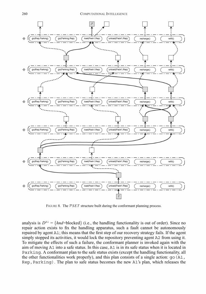
260 COMPUTATIONAL INTELLIGENCE
FIGURE 8. The PSET structure built during the conformant planning process.
analysis is DA1 = {hnd=blocked} (i.e., the handling functionality is out of order). Since norepair action exists to fix the handling apparatus, such a fault cannot be autonomouslyrepaired by agent A1; this means that the first step of our recovery strategy fails. If the agentsimply stopped its activities, it would lock the repository preventing agent A2 from using it.To mitigate the effects of such a failure, the conformant planner is invoked again with theaim of moving A1 into a safe status. In this case, A1 is in its safe status when it is located inParking. A conformant plan to the safe status exists (except the handling functionality, allthe other functionalities work properly), and this plan consists of a single action: go(A1,Rep,Parking). The plan to safe status becomes the new A1’s plan, which releases the
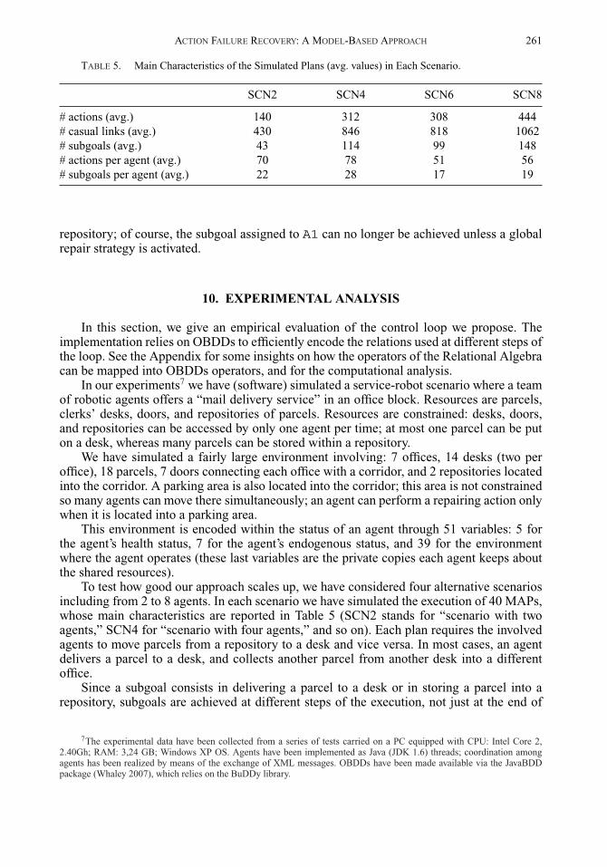
ACTION FAILURE RECOVERY: A MODEL-BASED APPROACH 261
TABLE 5. Main Characteristics of the Simulated Plans (avg. values) in Each Scenario.
SCN2 SCN4 SCN6 SCN8
# actions (avg.) 140 312 308 444# casual links (avg.) 430 846 818 1062# subgoals (avg.) 43 114 99 148# actions per agent (avg.) 70 78 51 56# subgoals per agent (avg.) 22 28 17 19
repository; of course, the subgoal assigned to A1 can no longer be achieved unless a globalrepair strategy is activated.
10. EXPERIMENTAL ANALYSIS
In this section, we give an empirical evaluation of the control loop we propose. Theimplementation relies on OBDDs to efficiently encode the relations used at different steps ofthe loop. See the Appendix for some insights on how the operators of the Relational Algebracan be mapped into OBDDs operators, and for the computational analysis.
In our experiments7 we have (software) simulated a service-robot scenario where a teamof robotic agents offers a “mail delivery service” in an office block. Resources are parcels,clerks’ desks, doors, and repositories of parcels. Resources are constrained: desks, doors,and repositories can be accessed by only one agent per time; at most one parcel can be puton a desk, whereas many parcels can be stored within a repository.
We have simulated a fairly large environment involving: 7 offices, 14 desks (two peroffice), 18 parcels, 7 doors connecting each office with a corridor, and 2 repositories locatedinto the corridor. A parking area is also located into the corridor; this area is not constrainedso many agents can move there simultaneously; an agent can perform a repairing action onlywhen it is located into a parking area.
This environment is encoded within the status of an agent through 51 variables: 5 forthe agent’s health status, 7 for the agent’s endogenous status, and 39 for the environmentwhere the agent operates (these last variables are the private copies each agent keeps aboutthe shared resources).
To test how good our approach scales up, we have considered four alternative scenariosincluding from 2 to 8 agents. In each scenario we have simulated the execution of 40 MAPs,whose main characteristics are reported in Table 5 (SCN2 stands for “scenario with twoagents,” SCN4 for “scenario with four agents,” and so on). Each plan requires the involvedagents to move parcels from a repository to a desk and vice versa. In most cases, an agentdelivers a parcel to a desk, and collects another parcel from another desk into a differentoffice.
Since a subgoal consists in delivering a parcel to a desk or in storing a parcel into arepository, subgoals are achieved at different steps of the execution, not just at the end of
7The experimental data have been collected from a series of tests carried on a PC equipped with CPU: Intel Core 2,2.40Gh; RAM: 3,24 GB; Windows XP OS. Agents have been implemented as Java (JDK 1.6) threads; coordination amongagents has been realized by means of the exchange of XML messages. OBDDs have been made available via the JavaBDDpackage (Whaley 2007), which relies on the BuDDy library.

262 COMPUTATIONAL INTELLIGENCE
TABLE 6. Monitoring under Nominal Conditions: CPU Time and OBDD Dimensions.
All four scenarios
CPU time [ms] action monitoring 11 ± 3 (avg.) 14 (max.)CPU time [ms] local plan monitoring 1072 ± 260 (avg.) 1355 (max.)# nodes within an agent belief 403 ± 20 (avg.) 635 (max.)# states within an agent belief 11 ± 2 (avg.) 16 (max.)# nodes within an action model 432 ± 82(avg.) 860 (max.)# state transitions within an action model 70 ± 26 (avg.) 129 (max.)
the plan. Of course, when agents execute their plans under nominal conditions, they achieveall their subgoals as the given MAP is assumed to be correct; otherwise, the occurrence ofa fault typically prevents the agents from achieving some of their subgoals; as we will see,a fault may have a huge impact affecting not only the agent where the fault occurs, but alsoother teammates. In the following analysis we use the number of achieved subgoals as ameasure both of the impact of a fault in the plan, and of the effectiveness of the proposedrepair strategy which tries to mitigate such an impact.
Table 6 reports relevant data about the execution of these plans under nominal conditions.Under this hypothesis, no time has been spent in the attempt of recovering from an actionfailure; thus we just show the average CPU time required by the monitoring phase in thefour scenarios. In fact the CPU time just depends on the sizes of the OBDDs encoding therelations mentioned in Definition 2 (namely, the agent belief state and the action model);while it does not depend on the number of agents involved in the team. It is evident thatthe monitoring activity is carried out very efficiently: estimating the belief state after theexecution of a single action is in the order of just 10 ms; such a time must be comparedto the actual time (in the order of seconds or even minutes) that a robotic agent takes forcompleting an action in the real world (service robots typically move very slowly especiallywhen they share the environment with humans).
Concerning the recovery problem, a key parameter to be set is the MAXDEPTHconstant. Such a value must be chosen taking into account that if it is too low, one canlose solutions; whereas if it is too high one could waste time looking for a solution thatdoes not exist, moreover a too long recovery plan may have a deleterious effect on the localplans of the other agents. In general, one can adopt some domain-dependent heuristics todetermine a reasonable value for MAXDEPTH. For instance, in our experiment we haveobserved that, according to the disposition of doors and resources, the longest round-tripfrom a resource to the parking area, including one repair action, requires 15 actions; so wehave set MAXDEPTH constant to 15.
To prove the effectiveness of our recovery strategy, we have perturbed each plan byrandomly injecting a fault in one agent’s functionality. Three typologies of faults have beenconsidered: repairable faults can autonomously be fixed by the agent through appropriaterepair actions; nonblocking faults cannot autonomously be repaired by the agent but theaffected agent may be able to move into a safe-status; finally, blocking faults have the worstimpact as the affected agent cannot even move into a safe-status. In our experiments we haveassumed that the first type of faults has a greater probability than the second one, which inturn is more probable than the last one. The chart in Figure 9 shows the distribution of faultsin the four scenarios.

ACTION FAILURE RECOVERY: A MODEL-BASED APPROACH 263
FIGURE 9. The distribution of faults over the four scenarios.
TABLE 7. SCN2 - Repair Costs: CPU Time in ms (in brackets the number of cases).
Repaired cases Cases moved to safe status Blocked cases
r + s 841 ± 129 [18 cases] 876 ± 138 [15 cases] 0 [7 cases]repair 838 ± 128 [18 cases] - 0 [22 cases]safe status - 112 ± 27 [33 cases] 0 [7 cases]no-repair - - −[40 cases]
The experimental evaluation has been conducted by comparing four alternative strategies.The first strategy, the easiest one, is no-repair: the agent in trouble does not react to an actionfailure, it just stops the execution of its local plan. The second strategy, called safe-status,aims at moving the agent in trouble into a safe-status after the occurrence of an action failure.In the third strategy, repair, the agent tries to repair its own plan by invoking the conformantre-planner, when the repair process fails the agent stops the plan execution. The last strategy,the one proposed in this paper, is a combination of the two previous strategies: first the agenttries to repair its plan, when this step fails the agent tries to move into a safe-status; thisstrategy will be denoted as r + s (repair + safe-status).
The efficiency of the different repair strategies has been measured by taking into accountboth the CPU time and the memory occupation (in terms of number of OBDD nodes). Table 7shows the CPU time spent by the conformant planner for synthesizing either a recovery planor a plan to safe status in SCN2. This time has been calculated according to the type of fault;for example, r+ s takes 841 ms (on average) when the case at hand is affected by a repairablefault; the same strategy takes a bit longer when it has to recover from a non-blocking faultas the conformant planner is invoked twice (first planning to R, and then planning to S). It

264 COMPUTATIONAL INTELLIGENCE
TABLE 8. SCN2 - Repair Costs: OBDDs Encoding � and PSET .
All four strategies
# nodes in � 6195 ± 697 (avg.) 7897 (max)# actions in � 36 ± 5 (avg.) 58 (max)CPU time to compute � [ms] 46 ±10 (avg.) 56 (max)
r + s
# nodes in P SET 288 ± 62 (avg.) 1351 (max)# repairing plans found 6 ± 2 (max) 33 (max)# repairing plan length 10 ± 3 (avg.) 14 (max)
TABLE 9. SCN4 - Repair Costs: CPU Time in ms (in brackets the number of cases).
Repaired cases Cases moved to safe status Blocked cases
r + s 841 ± 129 [18 cases] 876 ± 137 [15 cases] 0 [7 cases]repair 750 ± 200 [18 cases] - 0 [22 cases]safe status - 72 ± 25 [33 cases] 0 [7 cases]no-repair - - - [40 cases]
is worth noting that, when the fault is blocking, the strategy r + s does not waste time in avain search; this happens because the recovery strategy is driven by the agent diagnosis: it issufficient to include a blocking fault among the explanations to conclude that a conformantsolution does not exist. The table also reports the number of cases in which each strategy hasbeen activated successfully: the r+ s strategy successfully intervenes in all the 18 repairablefaults in this set of cases.
Table 8 shows the cost of the four strategies from the point of view of the dimensions(in terms of OBDD nodes) of two important structures: � and PSET . First of all, since� is built up by joining refined action models, its dimension is independent of the actualstrategy being used; moreover, even though � is a complex structure including a significantnumber of action models, the CPU time for computing it is almost negligible. The size ofPSET , on the other hand, which maintains the current set of plan candidates, depends onthe strategy being used; for brevity we just show some characteristics of this structure for ther + s strategy, captured when a solution has been found (i.e., when it gets the biggest size).Note that the dimension of PSET remains tractable in all the four scenarios (see Tables 10,12, and 14); this is an empirical demonstration that the r + s strategy is feasible in practiceeven though the theoretical computational cost of the conformant planner is exponential inthe length of the plan (see the Appendix).
The analysis of the repair strategies in scenarios SCN4, SCN6, and SCN8 is similar; theresults are showed in Tables 9–14.
The effectiveness of the four strategies is synthesized in Figure 10, reporting the averagenumber of plan actions performed by the agents in the four scenarios, and in Figure 11,where the percentage of achieved subgoals is showed. From the graphs it is apparent that r+s mitigates the harmful effects of a fault more effectively than the other strategies; in factwhen r + s is activated, the agents can perform more actions of the original plan, and hence

ACTION FAILURE RECOVERY: A MODEL-BASED APPROACH 265
TABLE 10. SCN4 - Repair Costs: OBDDs Encoding � and PSET .
All four strategies
# nodes in � 3945 ± 930 (avg.) 7932 (max)# actions in � 27 ± 6 (avg.) 58 (max)CPU time to compute � [ms] 46 ± 10 (avg.) 78 (max)
r + s
# nodes in PSET 177 ± 48 (avg.) 708 (max)# repairing plans found 3 ± 1 (max) 14 (max)# repairing plan length 10 ± 3 (avg.) 13 (max)
TABLE 11. SCN6 - Repair Costs: CPU Time in ms (in brackets the number of cases).
Repaired cases Cases moved to safe status Blocked cases
r + s 1009 ± 130 [18 cases] 1053 ± 135 [13 cases] 0 [9 cases]repair 1007 ± 146 [18 cases] - 0 [22 cases]safe status - 109 ± 34 [31 cases] 0 [9 cases]no-repair - - - [40 cases]
TABLE 12. SCN6 - Repair Costs: OBDDs Encoding � and PSET .
All four strategies
# nodes in � 6125 ± 1107 (avg.) 10,814 (max)# actions in � 33 ± 7 (avg.) 70 (max)CPU time to compute � [msec] 38 ± 6 (avg.) 93 (max)
r + s
# nodes in PSET 252 ± 53(avg.) 413 (max)# repairing plans found 4 ± 1 (max) 7 (max)# repairing plan length 9 ± 2 (avg.) 11 (max)
TABLE 13. SCN8 - Repair Costs: CPU Time in ms (in brackets the number of cases).
Repaired cases Cases moved to safe status Blocked cases
r + s 1677 ± 45 [20 cases] 1765 ± 47 [11 cases] 0 [9 cases]repair 1657 ± 35 [20 cases] - 0 [20 cases]safe status - 217 ± 34 [31 cases] 0 [9 cases]no-repair - - - [40 cases]
can achieve a greater number of subgoals. The chart in Figure 11 makes evident how theimpact of a fault is mitigated by r + s: when no-repair is active, the percentage of achievedsubgoals ranges from 40 to 63 in the four scenarios; this percentage rises to 71-84 whenr + s is active.

266 COMPUTATIONAL INTELLIGENCE
TABLE 14. SCN8 - Repair Costs: OBDDs Encoding � and PSET .
All four strategies
# nodes in � 9057 ± 1220 (avg.) 12,426 (max)# actions in � 37 ± 5 (avg.) 78 (max)CPU time to compute � [msec] 46 ± 7 (avg.) 94 (max)
r + s
# nodes in PSET 413 ± 62 (avg.) 529 (max)# repairing plans found 10 ± 2 (avg) 13 (max)# repairing plan length 10 ± 3 (avg.) 14 (max)
FIGURE 10. The average number of performed actions in the four scenarios: comparison between the repairstrategies and the nominal situation.
Of course, r + s requires more CPU time than other strategies, but the difference withrepair is very small; safestatus is cheaper than r + s and repair but its effects are limited;finally, no-repair is the cheapest, but, as expected, reaches the worst results.
From this analysis we can conclude that:
1. the monitoring process can be considered on-line as it is sufficiently efficient to followthe actual execution of an action performed by a robotic agent;
2. both monitoring and repair are able to deal with environments involving a significantnumber of resources;

ACTION FAILURE RECOVERY: A MODEL-BASED APPROACH 267
FIGURE 11. The percentage of achieved subgoals by the four repair strategies with the four scenarios.
3. in the worst cases the repair strategy takes 1.6 s to find a repairing plan, this time is accept-able in many domains involving mobile service-robots which, for safety requirements,typically move very slowly;
4. the number of actions within � (up to 78) demonstrates that our conformant planner isable to deal with nontrivial planning problems.
11. RELATED WORKS
There are two main research areas related to the work presented in this paper: planexecution monitoring and diagnosis and plan repair. The approach we have discussed, infact, represents a first step for the integration of plan execution and plan repair within a singlemodel-based framework. We start our discussion on related works by considering the planrepair area since the motivations of this work stems from that area.
In addressing the plan repair problem, a fundamental question must be answered: whatis the best solution between synthesizing a new plan from scratch and adapting the existing(failed) plan? Despite Nebel and Koehler (1995) have shown that plan adaptation representsa real advantage with respect to planning from scratch only when it reuses as much of theoriginal plan as possible, many researchers believe that plan adaptation still deserves tobe investigated, and a number of plan adaptation approaches have been proposed, see forexample PRODIGY/ANALOGY (Veloso et al. 1995), SPA (Hanks and Weld 1995), PRIAR(Kambhampati and Hendler 1992), GPG (Gerevini and Serina 2000).
The term plan adaptation comes from the case-based planning area, and refers to theprocess of modifying an existing plan π to solve a new problem, which is similar to the onesolved by π ; for instance, the old problem and the new one only differ for few facts in theinitial and goal states. Thus the original intent of plan adaptation is to solve a new planningproblem rather than repairing an existing plan (see e.g., Francis and Ram 1995; Hanks andWeld 1995; Hammond 1986; Kambhampati 1990).
More recent works (e.g., van der Krogt and de Weerdt 2005a; Cushing and Kambhampati2005; Fox et al. 2006) advocate that plan adaptation can be exploited to get robust planexecution in dynamic domains. These works, in fact, point out that plans are in general

268 COMPUTATIONAL INTELLIGENCE
synthesized by using abstract models of the worlds where they are going to be executed;since these abstract models just approximate the real world, discrepancies between theexpected status of the world (as predicted by the models), and the actual one may be detectedwhen a plan is actually executed. To cope with the new, unexpected conditions, the old planmust be replaced by a new one (i.e., the old plan needs to be repaired).
van der Krogt and de Weerdt (2005a) propose a basic template for plan repair, whichincludes two basic steps: first, actions that prevent the achievement of the goal(s) are removed;and then, actions that bring the agent closer to the goal(s) are introduced. The first phase isalso called plan unrefinement, whereas the second one is called plan refinement (see alsoKambhampati 1997). Plan unrefinement is driven by a heuristic to find an appropriate portionof the plan to be removed; whereas, plan refinement consists of a planning process that hasto fill the gaps left by the unrefinement step.
In the approach we have discussed we do not have an explicit phase of plan unrefinement.However, the planning phase can implicitly realize this step by including into the repairingplan actions which compensate the effects of actions that have already been executed. In theexample discussed in Section 9, for instance, both the two repairing solutions start with anunload action which compensate the effect of a previous load.
In Fox et al. (2006), the authors introduce the notion of plan stability as a metric to assessthe quality of a repaired plan. In fact, when the repaired plan is close to the original one it iseasier for humans to understand the changes. Moreover, a plan is also a way to communicatefuture intentions to other agents and, to do this successfully, the repaired plan should be asclose as possible to the original one (Cushing and Kambhampati 2005; Cushing, Benton,and Kambhampati 2008).
Since an agent is typically situated in an environment shared with other agents, someauthors have addressed the problem of plan repair in a multi-agent setting. van der Krogtand de Weerdt (2005b) discuss a planning methodology where self-interested agents achieveglobally consistent local plans by means of an iterative plan repair process. In their approacheach agent infers a local plan autonomously, during this process the agent can either decideto achieve a goal by itself or to ask some other agent for it. When an agent accepts to achievea goal for another agent, it has to change its original plan to include among its goals the newone; its local plan is therefore adapted (i.e., repaired) to this end. The methodology is veryinteresting but introduces some assumptions which make it unsuitable for our scenario; forexample, it is assumed that agents cannot share resources and that agents have a completeknowledge about its own problem. Both assumptions are acceptable during a planning phase,but they are not in plan execution.
Another approach to multiagent replanning is discussed in Zhang, Nguyen, andKowalczyk (2007); the authors present a distributed refinement strategy to construct a graphplan fixing errors occurred during the execution of a MAP; this work, however, does not takeinto account that failures may be due to faults in the agent’s functionalities.
Extensions of Markov Decision Processes (MDPs) have also been proposed to solve theproblem of coordinating a team of agents. For example, Decentralized MDPs (Dec-MDPs)have been proposed in Bernstein et al. (2002) to model teams of agents that operate undercollective observability. Collective observability is a condition where, although each agentis unable to independently identify the global world state, the union of all the observationsreceived by the team members at a given time yield a fully observed state. Other approachesare based on factored MDPs (Boutilier, Dearden, and Goldszmidt 2000; Guestrin, Koller,and Parr 2001; Guestrin and Gordon 2002); while standard MDPs enumerate all the possiblestates, factored MDPs take advantage of conditional independencies among state variablesand yield more compact state representations, and possibly more compact policies. Although

ACTION FAILURE RECOVERY: A MODEL-BASED APPROACH 269
these approaches are mainly concerned with the planning problem in a multiagent scenario,they could also be adopted to solve the plan repair problem.
The literature on the second area of interest, the plan execution monitoring, is verybroad; seminal studies on this topic come from the field of industrial control, where it isoften referred to as the problem of fault detection and isolation (FDI; Pettersson 2005). Sincethe end of 1970s, a number of monitoring methodologies have been validated in industrialapplications see Gertler (1998) and Chen and Patton (1999) for an overview.
Roughly speaking, execution monitoring in robotics can be categorized into two mainfamilies of approaches: model-based and model-free. In model-based approaches, a model ofthe system (robot and environment) is used to generate expectations about the nominal behav-ior of the robot; these expectations are subsequently compared to the available observationsreceived during the actual execution to detect discrepancies. Examples of architectures inthis category include, among others, the Remote Agent by Muscettola, Nayak, and Williams(1998), the LAAS proposal (Alami et al. 1998) and ROUGE (Haigh and Veloso 1998).Model-free approaches, on the other hand, do not use predictive models, but pattern recog-nition mechanisms to learn on-line both nominal and faulty behaviors (Pettersson, Karlsson,and Saffiotti 2003, 2005). It is easy to see that the present paper falls into the first category.
Most of the approaches in the literature assume that action failures are consequencesof unexpected environment conditions; in this paper we adopt a vision similar to the onediscussed in Birnbaum et al. (1990), where the outcome of an action is related to the healthstatus of the agent performing it. A nonnominal action outcome is therefore explained interms of domain-dependent threats which have affected the health status of the agent. Inour work, plan threats are faults in the agent’s functionalities; the proposed extended actionmodels capture the relation between the agent health status and action outcomes.
The work by Birnbaum et al. has been recently extended to the multiagent scenario.To the best of our knowledge, however, only a few approaches tackle plan execution mon-itoring and diagnosis in a multi-agent scenario. In Roos and Witteveen (2009) the authorsconsider the MAP as the system to be diagnosed, and hence they introduce the notion ofplan diagnosis as the subset of actions whose failure is consistent with the anomalous ob-served behavior of the system; thus this work just focuses on the detection of abnormalactions. In de Jonge et al. (2009) the same authors complement plan diagnosis with thenotion of secondary diagnosis. More precisely, while the plan diagnosis is the primary di-agnosis identifying the failed actions; the secondary diagnosis explains why those actionshave failed. Roos et al. distinguish three possible secondary plan diagnoses: agent diagnosis(faults in the agent’s functionalities), equipment diagnosis (faults in the resources used bythe agents), and environment diagnosis (unexpected changes in the environment). To achievethis result, the authors exploit action models which share some similarities with the extendedmodels we have proposed; in fact, their action models explicitly mention the functionali-ties and resources required for the successful completion of the action; moreover, knownfaulty models of the agent’s functionalities can be used to partially predict the next agentstatus.
At the current stage of development, the portion of our framework related to plandiagnosis is a subset of the framework by Roos et al. But in this work we are more interestedin the whole control loop from detection to recovery, and we have considered here justthe agent diagnosis to simplify the discussion. Nonetheless, Roos et al. have opened someappealing research lines along which our strategy could be extended. Indeed, we have startedworking on diagnosing failures caused by unexpected changes in the environment, seeMicalizio and Torasso (2008, 2009). From the recovery point of view, however, the controlstrategy must still be extended to deal with unexpected exogenous events. For instance, a

270 COMPUTATIONAL INTELLIGENCE
new general strategy must be conceived to match an exogenous event with a recovered stateto be reached in order to recover from a failure.
A different notion of diagnosis is the one discussed in Kalech and Kaminka (2007,2011) where the authors introduce the social diagnosis to find out the cause of coordinationfailures. In their approach the authors do not explicitly consider plans, they rather model ahierarchy of behaviors: each agent selects independently from others the more appropriatebehavior given its own beliefs. When an agent selects a behavior which is not in accordancewith the ones selected by its teammates, a disagreement has been detected, and a diagnosticprocess is activated to determine its root causes. In this case, the social diagnosis explainsthe disagreement by individuating portions of the agents’ beliefs which are one another inconflict.
12. SUMMARY AND CONCLUSIONS
Cushing and Kambhampati (2005) have observed that, to repair a plan after the occur-rence of an action failure, one has to consider not only the unexpected changes occurred inthe environment, but also faults affecting the agent’s functionalities. In their opinion, thus,a repair strategy has to get two results: on the one side, it must adjust the original planaccording to new environment conditions; on the other side, it must also fix (if possible) theagent’s faults.
The paper originates from this observation and represents an attempt of complementingprevious works on plan repair (see, e.g., van der Krogt and de Weerdt 2005a; Fox et al. 2006),which typically assume that the agent is fault-free and that the causes of an action failure aredue to the environment. In this work, we have focused on those situations where an actionfailure is due to faults, and we have proposed a recovery strategy which aims at restoring ahealthy status in the agent’s functionalities.
The paper points out some important challenges one has to face to solve the problem ofaction failure recovery. First of all, there is the need of detecting action failures and relatingthem to faults. Since the nominal action models used during the planning phase are inadequatefor this purpose, we have introduced extended action models which allow a mapping betweenfaults and action failures. However, since faults may have non-deterministic effects, mappingan action failure with a fault is not a trivial task as a number of alternative explanations maybe possible. To cope with this problem, the paper adopts techniques from the MBD fordetecting and diagnosing action failures. Finally, since faults and their contextual conditionsare difficult to anticipate, it is not possible to exploit precompiled recovery solutions; sothe paper presents a recovery strategy, which based on a conformant planner and drivenby the agent diagnosis, synthesizes on-the-fly a recovery plan fixing the (assumed) faultyfunctionalities.
The paper contributes to the plan repair area in a number of ways. First of all, it presentsin a formal way a unique framework where three main activities—monitoring, diagnosis, andrecovery—are integrated with one another within a closed loop of control. The frameworkhas been discussed in terms of relations and Relational Algebra operators between relations.This language has two important advantages: (1) it is easy to define extended action modelswith non-deterministic effects in terms of relations; (2) it allows a declarative presentationof the control loop.
A further contribution of the paper is that the recovery strategy, albeit conceived fora single agent, can successfully be adopted within a multi-agent setting. As noticed byRoth, Simmons, and Veloso (2007), in fact, in many multi-agent domains agents operateindependently of one another for long periods and coordinate their actions in just fewoccasions. The basic idea of our strategy is to intervene in the plan segments where an

ACTION FAILURE RECOVERY: A MODEL-BASED APPROACH 271
agent operates isolated from others; the recovery, however, preserves the plan segmentswhere the agent interacts with other team members. Therefore, when the recovery terminatessuccessfully, only the plan of the agent in trouble has been changed, and this change iscompletely transparent to the other members of the team.
12.1. Limits of the Framework and Future Developments
The proposed local strategy is meant to be a first attempt to overcome an action failuretrying to change the plan of the impaired agent only. When a recovery plan does not exist,the impaired agent tries to move into a safe status where it does not represent a menace forother agents. It may be possible, however, that such a safe status is not achievable or evenmissing; in that case the faulty agent gets stuck and locks a subset of resources indefinitely.A possible way to overcome this limitation consists in complementing the local strategy witha team-based strategy, where agents cooperate with one another to overcome a single failure.In particular, in a team-based strategy agents would be able to acquire and release resourcesfreely, without the limitations imposed by the locality requirement. This would help an agentto build a recovery plan by acquiring new resources. Moreover, when a recovery plan doesnot exist, the faulty agent could coordinate with the other teammates to move from place toplace without locking resources indefinitely. In other words, the safe status of a faulty agentwould not be a place where it can isolate itself, but a high-level goal achieved by a form ofcontinual planning.
The work by van der Krogt and de Weerdt (2005b) discusses an interesting approach toplan repair in a multiagent scenario where agents negotiate goals and services, however, thework introduces some assumptions which make the approach not directly applicable in ourscenario. For instance, the authors assume that the problems of all the agents are mutuallydistinct, meaning that agents cannot use the same resources. Of course, this assumption canbe hardly applied in a service-robots scenario, where resources are actually shared and agentsare typically involved in conflicts/negotiations for accessing them. An interesting researchline is to extend the framework by van der Krogt et al. to relax their assumptions and meetour scenario.
Another possible extension is about the agent diagnosis. In the current solution therecovery mechanism tries to find a plan fixing all the faults assumed by the agent diagnosis,which in general is ambiguous. Thereby some of the repairing actions included within therecovery plan are not really necessary. Redundant repairing actions may represent an issueespecially when they are expensive and time consuming. A possible solution to mitigate theproblem could be the adoption of “active diagnosis” techniques to refine the ambiguous agentdiagnosis. The basic idea of active diagnosis is to perform a number of actions intended totest the agent’s functionalities assumed to be faulty: test actions are therefore used to confirmor disconfirm the hypotheses made by the agent diagnosis. Of course, active diagnosistechniques do not guarantee to precisely identify the actual fault affecting an agent, but theycan significantly reduce the ambiguity of the agent diagnosis, and hence reduce the numberof redundant repairing actions in the recovery plan.
REFERENCES
ALAMI, R., R. CHATILA, S. FLEURY, M. GHALLAB, and F. INGRAND. 1998. An architecture for autonomy.International Journal of Robotics Research, 17(4):315–337.
BERNSTEIN, D., R. GIVAN, N. IMMERMAN, and S. ZILBERSTEIN. 2002. The complexity of centralized control ofmarkov decision processes. Mathematics of Operations Research, 27(4):819–840.

272 COMPUTATIONAL INTELLIGENCE
BIRNBAUM, L., G. COLLINS, M. FREED, and B. KRULWICH. 1990. Model-based diagnosis of planning failures. InProceedings of the AAAI90, Boston, MA, pp. 318–323.
BOUTILIER, C., and R. I. BRAFMAN. 2001. Partial-order planning with concurrent interacting actions. Journal ofArtificial Intelligence Research, 14:105–136.
BOUTILIER, C., R. DEARDEN, and M. GOLDSZMIDT. 2000. Stochastic dynamic programming with factoredrepresentations. Artificial Intelligence, 121(1-2):49–107.
BRENNER, M., and B. NEBEL. 2009. Continual planning and acting in dynamic multiagent environments.Autonomous Agents and Multi-agent Systems, 19:297–331.
BRYANT, R. 1986. Graph-based algorithms for Boolean function manipulation. IEEE Transactions on Computers,35(8):677–691.
BRYANT, R. 1992. Symbolic Boolean manipulation with ordered binary-decision diagrams. ACM ComputerSurveys, 24:293–318.
CHEN, J., and R. PATTON. 1999. Robust Model-Based Fault Diagnosis for Dynamic Systems. Kluwer AcademicPublishers: Boston: MA.
CIMATTI, A., and M. ROVERI. 2000. Conformant planning via symbolic model checking. Journal of ArtificialIntelligence Research, 13:305–338.
CONSOLE, L., D. THESEIDER, and P. TORASSO. 1991. On the relation between abduction and deduction. Journalof Logic and Computation, 1(5):661–690.
CONSOLE, L., and P. TORASSO. 1991. Integrating models of correct behavior into abductive diagnosis. Computa-tional Intelligence, 7(3):133–141.
COX, J. S., E. H. DURFEE, and T. BARTOLD. 2005. A distributed framework for solving the multiagent plancoordination problem. In Proceedings of the International Conference on Autonomous Agents and Multi-Agent Systems (AAMAS’05), Utrecht, the Netherlands, pp. 821–827.
CUSHING, W., J. BENTON, and S. KAMBHAMPATI. 2008. Replanning as deliberative re-selection of objectives. InTechnical report. ASU CSE.
CUSHING, W., and S. KAMBHAMPATI. 2005. Replanning: A new perspective. In Poster Program of the InternationalConference on Automated Planning and Scheduling (ICAPS’05), Monterey, CA.
DARWICHE, A., and P. MARQUIS. 2002. A knowledge compilation map. Journal of Artificial Intelligence Research,17: 229–264.
DE JONGE, F., N. ROOS, and C. WITTEVEEN. 2009. Primary and secondary diagnosis of multi-agent plan execution.Journal of Autonomous Agents and Multi-Agent Systems, 18:267–294.
DECKER, K., and J. LI. 2000. Coordinating mutually exclusive resources using gpgp. Journal of AutonomousAgents and Multi-Agent Systems, 3(2):113–157.
DURFEE, E. H. 2001. Mutli-agent systems and applications. Springer-Verlag: New York.
FIKES, R., and N. NILSSON. 1971. Strips: A new approach to the application of theorem proving to problemsolving. Artificial Intelligence, 2(3-4):189–208.
FOX, M., A. GEREVINI, D. LONG, and I. SERINA. 2006. Plan stability: Replanning versus plan repair. In Proceedingsof the International Conference on Automated Planning and Scheduling (ICAPS’06), Lake District, UK,pp. 212–221.
FOX, M., and D. LONG. 2003. Pddl2.1: An extension to pddl for expressing temporal planning domains. Journalof Artificial Intelligence Research, 20:61–124.
FRANCIS, A. G., Jr., and A. RAM. 1995. A domain-independent algorithm for multi-plan adaptation and merging inleast-commitment planners. In AAAI Fall Symposium: Adaptation of Knowledge Reuse, MIT, Cambridge,MA, pp. 19–25.
GEREVINI, A., and I. SERINA. 2000. Fast plan adaptation through planning graphs: local and systematic searchtechniques. In Proceedings of the International Conference on Artificial Intelligence Planning and Schedul-ing (AIPS’00), Breckenridge, CO, pp. 112–121.
GERTLER, J. 1998. Fault Detection and Diagnosis in Engineering Systems. CRC Press: New York.

ACTION FAILURE RECOVERY: A MODEL-BASED APPROACH 273
GHALLAB, M., A. HOWE, C. KNOBLOCK, D. MCDERMOTT, A. RAM, M. VELOSO, D. WELD, and D. WILKINS.1998. Pddl - the planning domain definition language. In Proceedings of the International Conference onArtificial Intelligence Planning and Scheduling, Carnegie Mellon University, Pittsburgh, PA.
GUESTRIN, C., and G. GORDON. 2002. Distributed planning in hierarchical factored mpds. In Proceedings of theEighteenth Conference on Uncertainty in Artificial Intelligence, University of Alberta, Edmonton, Canada,pp. 197–206.
GUESTRIN, C., D. KOLLER, and R. PARR. 2001. Multiagent planning with factored mdps. In Proceedingsof the Advances in Neural Information Processing Systems (NIPS’01), Vancouver, Canada, pp. 1523–1530.
HAIGH, K., and M. VELOSO. 1998. Planning, execution and learning in a robotic agent. In Proceedings of theInternational Conference on Artificial Intelligence Planning and Scheduling, Carnegie Mellon University,Pittsburgh, PA, pp. 120–127.
HAMMOND, K. J. 1986. Chef: A model of case-based planning. In Proceedings of the AAAI, Philadelphia, PA,pp. 267–271.
HANKS, S., and D. WELD. 1995. A domain-independent algorithm for plan adaptation. Journal of ArtificialIntelligence Research (JAIR), 2:319–360.
JENSEN, R. M., and M. M. VELOSO. 1999. Obdd-based universal planning: Specifying and solving planningproblems for synchronized agents in non-deterministic domains. LNCS, 1600:213–249.
JENSEN, R. M., and M. M. VELOSO. 2000. Obdd-based universal planning for synchronized agents in non-deterministic domains. Journal of Artificial Intelligence Research, 13:189–226.
KALECH, M., and G. A. KAMINKA. 2007. On the design of coordination diagnosis algorithms for teams of situatedagents. Artificial Intelligence, 171:491–513.
Kalech, M., and G. A. Kaminka. 2011. Coordination diagnostic algorithms for teams of situated agents: Scalingup. Computational Intelligence, 27(3):383–421.
KAMBHAMPATI, S. 1990. Mapping and retrieval during plan reuse: A validation structure based approach. InProceedings of the AAAI, Boston, MA, pp. 170–175.
KAMBHAMPATI, S. 1997. Refinement planning as a unifying framework for plan synthesis. AI Magazine, 18(2):67–97.
KAMBHAMPATI, S., and J. HENDLER. 1992. A validation structure based theory of plan modification and reuse.Artificial Intelligence, 55:193–258.
LAM, M., S., J. WHALEY, V. B. LIVSHITS, C. Martin, M., D. AVOTS, M. CARBIN, and C. UNKEL. 2005. Context-sensitive program analysis as database queries. In Proceedings of the twenty-fourth ACM SIGMOD Sym-posium on Principles of Database Systems, Baltimore, MD, pp. 1–12.
Lhotak, O., and L. HENDREN. 2004. Jedd: A bdd-based relational extension of java. SIGPLAN Not., 39:158–169.
Lind-Nielsen, J. 2003. Buddy: A binary decision diagram package. Available at: http://vlsicad.eecs.umich.edu/BK/Slots/cache/www.itu.dk/research/buddy/index.html/. Accessed May 28, 2012.
MICALIZIO, R., and P. TORASSO. 2008. Monitoring the execution of a multi-agent plan: Dealing with partialobservability. In Proceedings of the European Conference on Artificial Intelligence (ECAI’08), Patras,Greece, pp. 408–412.
MICALIZIO, R., and P. TORASSO. 2009. Agent cooperation for monitoring and diagnosing a map. In MultiagentSystem Technologies, 7th German Conference, MATES, Vol. 5774 of LNCS, Hamburg, Germany, pp.66–78.
MUSCETTOLA, N., P. NAYAK, and B. WILLIAMS. 1998. Remote agent: To boldly go where no AI system has gonebefore. Artificial Intelligence, 103:5–47.
NEBEL, B. 2000. On the compilability and expressive power of propositional planning formalisms. Journal ofArtificial Intelligence Research, 12:271–315.
NEBEL, B., and J. KOEHLER. 1995. Plan reuse versus plan generation: A theoretical and empirical analysis.Artificial Intelligence, 76(1):427–454.

274 COMPUTATIONAL INTELLIGENCE
PEOT, M., and D. E. SMITH. 1992. Conditional nonlinear planning. In Proceedings of the International Conferenceon Artificial Intelligence Planning and Scheduling(AIPS’92), College Park, MD, pp. 39–46.
PETTERSSON, O. 2005. Execution monitoring in robotics: A survey. Robotics and Autonomous Systems, 53:73–88.
PETTERSSON, O., L. KARLSSON, and A. SAFFIOTTI. 2003. Model-free execution monitoring in behavior-basedmobile robotics. In Proceedings of the International Conference on Advanced Robotics (ICAR), Coimbra,Portugal, pp. 864–869.
PETTERSSON, O., L. KARLSSON, and A. SAFFIOTTI. 2005. Model-free execution monitoring by learning fromsimulation. In Proceedings of the Computational Intelligence in Robotics and Automation (CIRA), Espoo,Finland, pp. 505–511.
REITER, R. 1987. A theory of diagnosis from first principles. Artificial Intelligence, 32(1):57–96.
ROOS N., and C. WITTEVEEN. 2009. Models and methods for plan diagnosis. Journal of Autonomous Agents andMulti-Agent Systems, 19(1):30–52.
ROTH, M., R. SIMMONS, and M. VELOSO. 2007. Exploiting factored representations for decentralized execution inmulti-agent teams. In Proceedings of the International Conference on Autonomous Agents and Multi-AgentSystems (AAMAS’07), Honolulu, HI, pp. 469–475.
TORTA G., and P. TORASSO. 2007. On the role of modeling causal independence for system model compilationwith obdds. AI Communications, 20(1):17–26.
van der Krogt, R., and M. DE WEERDT. 2005a. Plan repair as an extension of planning. In Proceedings of the15th International Conference on Automated Planning and Scheduling (ICAPS’05), Monterey, CA, pp.161–170.
van der Krogt, R., and M. DE WEERDT. 2005b. Self-interested planning agents using plan repair. In Proceedingsof the 15th International Conference on Automated Planning and Scheduling (ICAPS’05), Monterey, CA,pp. 36–44.
VELOSO M., J. CARBONELL, A. Perez, D. BORRAJO, and J. BLYTHE. 1995. Integrating planning and learning: Theprodigy architecture. Journal of Experimental and Theoretical Artificial Intelligence, 7:189–197.
WELD, D. S. 1994. An introduction to least commitment planning. AI Magazine, 15(4):27–61.
WHALEY, J. 2007. Javabdd package - project summary page at http://javabdd.sourceforge.net. Accessed May 28,2012.
ZHANG, J. F., X. T. NGUYEN, and R. KOWALCZYK. 2007. Graph-based multi-agent replanning algorithm. In Pro-ceedings of the International Conference on Autonomous Agents and Multi-Agent Systems (AAMAS’07),Honolulu, HI, pp. 798–805.
APPENDIX A: RELATIONAL ALGEBRA OPERATORS
This appendix summarizes some basic notions about relations and operators of theRelational Algebra.
A relation R consists of a schema Rσ and of a set of contained tuples Rτ . The schema isan ordered list of attributes, or variables, Rσ = 〈v1, . . . , vn〉, where each variable vi (i : 1..n)has a finite domain dom(vi ). Each tuple t = 〈d1, . . . , dn〉 in Rτ represents an assignmentof values to the variables in the relation schema such that di ∈ dom(vi ) for each i : 1..n(namely, t ∈ dom(v1)× · · · × dom(vn)).
The Relational Algebra operators we are interested in are:
1. union: given two relations R and S defined over the same set of attributes (Rσ equalsSσ ); the union R ∪ S is a new relation T , defined on the same set of attributes as R andS, containing all the tuples of R and all the tuples of S without duplicates; formally:Tσ = Rσ = Sσ , and Tτ = Rτ ∪ Sτ .

ACTION FAILURE RECOVERY: A MODEL-BASED APPROACH 275
2. intersection: given two relations R and S defined over the same set of attributes; theintersection R ∩ S is a new relation T , having the same schema as R and S, and containingthe tuples which belong both to R and to S: Tτ = Rτ ∩ Sτ . Of course, T might result tobe empty.
3. difference: given two relations R and S defined over the same set of attributes; thedifference R − S is a new relation T , having the same schema as R and S, and containingthe tuples which belong to R but which do not appear in S: Tτ = Rτ − Sτ .
4. Cartesian product: given two relations R and S defined over schemas which are oneanother disjointed (Rσ ∩ Sσ = ∅), the Cartesian product R × S is a new relation T suchthat:
(i) Tσ = Rσ ∪ Sσ
(ii) Tτ = Rτ × Sτ = {t is a tuple in Tτ such that t = t1 ∪ t2,∀ t1 ∈ Rτ ,∀ t2 ∈ Sτ }: eachtuple in R is combined with each tuple in S, the result is stored in T.
5. select: given a relation R and a predicate ρ, SELECTρ R is a new relation T such that:
(i) T has the same schema as R(ii) each tuple in Tτ satisfies the predicate ρ
ρ is defined over (a subset of) the schema variables, and typically represents arestriction of the domains of these variables.
6. project: given a relation R and a subset γ ⊆ Rσ of variables , PROJECTγ R is a new relationT such that:
(i) Tσ = γ(ii) Tτ is the projection of Rτ over the variables in γ : all the variables which are not in γ
are discarded, duplicated tuples are removed.
7. join: in the paper we only utilize the natural-join operator, which is a specific case ofjoin, for brevity however we use the generic term join. Let R and S be two relations suchthat Rσ ∩ Sσ = ∅ (the two relations share a subset of variables); let ω be such a subset ofshared variables. The (natural) join operation, denoted as R JOIN S, is the new relation Tdefined as:
(i) Tσ = Rσ ∪ Sσ (without duplication of variables)(ii) Tτ = {t is a tuple | t = t1 ∪ t2, ∀ t1 ∈ Rτ , ∀ t2 ∈ Sτ , such that ∀v ∈ ω, t1(v) = t2(v)}
The natural join combines a tuple t1 in R with a tuple t2 in S only when the two tuplesare related to each other as they assign the same values to the shared variables in ω.
APPENDIX B: COMPUTATIONAL ANALYSIS
In this work we have presented in a declarative manner a methodology to control theexecution of a plan by integrating model-based diagnosis and conformant planning. Boththese activities have been formalized in terms of relations and operations between relations.
The computational complexity of the proposed algorithms strongly depends on howefficiently these relations are handled; any operation on relations, in fact, can easily become

276 COMPUTATIONAL INTELLIGENCE
TABLE 15. OBDD Operators and Their Complexity.
Operator Result Time Size
Reduce( f ) G reduced to canonical form O(|G| · log |G|) |G|Apply(op, f1, f2) f1〈op〉 f2 O(|G1| · |G2|) |G1| · |G2|Restrict(xi , b, f ) f |xi=b O(|G|) ≤ |G|
a bottleneck. Before addressing the computational analysis, it is therefore necessary to brieflydiscuss how the algorithms have been implemented.
Basic Concepts on OBDDs
We have adopted the formalism of the Ordered Binary Decision Diagrams (OBDDs;Bryant 1986) to symbolically, and hence compactly, encode the relations involved in thecontrol strategy. OBDDs are a well-known mathematical tool, which compactly encodecomplex Boolean functions as rooted DAGs having only two leaves: zero (i.e., false) andone (i.e., true). While OBDDs have initially been developed to test hardware failures, they arebecoming widely used in many areas of the Artificial Intelligence for efficiently representingand manipulating large state spaces (see, for instance, diagnosis of component-based systems(Torta and Torasso 2007), and different kind of planning (Cimatti and Roveri 2000; Jensenand Veloso 2000)). Some basic operators on OBDDs are reported in Table 15 (see also Bryant1986). In the table, the Boolean function f is represented by a reduced function graph Gcontaining |G| vertices; similarly for the functions f1 and f2. The meaning of these operatorsis as follows:
1. the reduce operator gets the canonical form of a Boolean function f ; that is, given aspecific variables ordering, the reduce operator gets a graph G whose size is minimal.
2. the binary logical operations between two Boolean functions f1 and f2 is realized bythe apply operator working on the graphs G1 and G2, respectively encoding the twofunctions. The computational complexity in the worst case is the product of the sizes(i.e., number of vertices) of the two graphs.
3. the restrict operator substitutes a constant b to a variable xi in linear time in the numberof vertices.
The adoption of the OBDDs is not a per se panacea; since the computational complexityof the OBDDs operators depends on the sizes of the involved OBDDs, it is important toget minimal-size OBDDs. However, the size of an OBDD depends on the variable orderingchosen during the reduce operation, a wrong variable ordering may result in an exponentialgrowth of the OBDD size. It has been demonstrated that finding an optimal variable orderingminimizing the size of an OBDD is a NP-hard problem. Heuristics are typically used tocope with this issue; for instance, many approaches keep close variables which depend onone another (Jensen and Veloso 1999; Torta and Torasso 2007).
The problem of how translating a relation into an OBDDs has been addressed in previousworks (Bryant 1992; Lhotak and Hendren 2004). In this paper we just give some hints onhow to solve it. First of all, we observe that any n-ary relation R can be encoded as a Boolean
ACTION FAILURE RECOVERY: A MODEL-BASED APPROACH 277
function fR:
f (d1, . . . , dn) ={
1 if 〈d1, . . . , dn〉 ∈ R[τ ]0 otherwise.
For instance, given the belief state in Table 2, the corresponding Boolean func-tion is defined as fbelie f : dom(pos)× dom(loaded)× dom(pwr )× dom(engTmp)×dom(hnd)→ {0, 1}, and it assumes the value 1 only for the two combinations of valuesreported in the table, namely, 〈 Rep, Pack1, ok, high, ok 〉 and 〈 Rep, Pack1, low , ok,ok 〉; the function is 0 for any other combination of values. By means of a proper renamingof variables, also the relations representing action models (which report the same statusvariables at two consecutive time instants) can be translated into Boolean functions. Forinstance, the extended model of action go (see Table 1) is modeled by the Boolean function
fgo : dom(pos)× dom(loaded)× dom(pwr )× dom(engTmp)×
dom(posNxt)× dom(loadedNxt)× dom(pwrNxt)× dom(engTmpNxt)→ {0, 1}.
As in the previous case, the function fgo assumes the value true for each combination ofvalues corresponding to an entry of Table 1, false in any other case.
Note that we have heuristically chosen the variable ordering {pos, pos N xt , loaded,loaded N xt . . .} to obtain an OBDD Ggo efficiently encoding the Boolean function fgo; infact, the value of a “next” variable will strongly depend on the value of the corresponding“current” variable.
Once we have translated each relation into a Boolean function, we can observe thateach operator of the Relational Algebra can be mapped to an operation (or a combinationof operations) between Boolean functions (see Lam et al. 2005). Consider for example thepredictive step of the monitoring process, realized by a JOINoperator between the currentbelief state and the action model, this step is translated into the Boolean expression fbelie f ∧fgo.
Note also that some of the packages implementing OBDDs provide useful operatorswhich correspond to a sequence of Relational operations. For instance, natural join operationsare frequently followed by project operations to eliminate unnecessary attributes. The OBDDoperation relprod, provided by the BuDDy package (Lind-Nielsen 2003), efficientlycombines this sequence in a single operation. Similarly, the select and project operations canbe combined into a single restrict operation between OBDDs (Lam et al. 2005).
Computational Analysis
In this section we discuss separately the computational complexity of the three maintasks (monitoring, diagnosis, and recovery) included within the proposed control strategy bytaking into account their OBDD-based implementation.
Plan Execution Monitoring. The main goal of the monitoring activity consists in esti-mating the agent belief state Bi (t + 1) given the previous belief state Bi (t) and the extendedmodel of action ai
l (t). This process has been formalized in Definition 2. To assess the com-putational complexity of such a process, we have first to consider how it is actually translatedinto OBDD operators. Let Gbelie f be the OBDD encoding Bi (t), Gaction be the OBDD en-coding the model of action ai
l (t), and Gobs be the OBDD encoding the available observations

278 COMPUTATIONAL INTELLIGENCE
obsi (t + 1); then the Relational expression
SELECTobs i (t+1)(Bi (t)JOIN �(ail (t)) (B.1)
is translated into the following expression on OBDDs:
Gint = apply(∧, Gobs , apply(∧, Gbelie f , Gaction)), (B.2)
where Gint is the intermediate OBDD resulting from the two subsequent apply operations.Relying on Table 15, we can conclude that the complexity for getting Gint is
O(|Gbelie f | · |Gaction| · |Gobs |). (B.3)
The last relational operation to obtain the belief stateBi (t + 1) is the projection over the statusvariables in VARi
t+1 (i.e., the “next” variables ). To remove a variable v from an OBDD onecan exploit the restrict operation, in particular, one has to invoke the restrict operator for eachvalue in dom(v). The projection is therefore translated into a number of restrict operationsover Gint , which is proportional to the number of variables to be discarded (namely, thevariables in VARi
t ), and to the cardinality of the variable domains. Let maxDomSize =argmaxv∈VARi |dom(v )| be the greatest domain cardinality; the computational cost for theprojecting Gint over VARi
t+1 is
O(maxDomSize · |VARi | · |Gint |). (B.4)
Although this computational result might not appear completely satisfactory, it is importantto note that it is an estimation of the very worst case. Bryant himself states that this theoreticalcomplexity is not so frequent in practice, and he conjectures that the actual complexity ofan apply operation between two OBDDs G1 and G2 is O(|G1| + |G2| + |G3|), where G3 isthe resulting OBDD (Bryant 1986). Indeed, the experimental results discussed in Section 10have shown that the monitoring process is actually carried out very efficiently and that thesize of the OBDDs encoding the agent belief states and the action models are kept small.
Agent Diagnosis. The inference of the agent diagnosis in Relational terms is given inDefinition 4, it simply consists in a projection of the belief state Bi (t + 1) over the healthstatus variables. Let Gnew Belie f be the OBDD encoding such an agent belief state; thecomputational complexity for projecting Gnew Belie f over the variables in healthVar(ai
l ) is
O(maxDomSize · |VARi \ healthVar (a il ) | · |GnewBelief |). (B.5)
In fact, also in this case the projection is translated into a number of restrict operations whichis proportional to the number of variables that must be removed and to the size of theirdomains.
Recovery. The recovery strategy is formalized in the algorithm of Figure 6; this algorithmfirst determines which goal must be reached (either R or S), and then invokes the conformantplanner trying to find a plan getting the desired goal. It is easy to see that the real complexityof the recovery process is in the solution of a conformant planning problem rather than inthe recovery strategy itself; for this reason, we will only examine the computational cost ofthe conformant planner.
The pseudo-code of the conformant planner is given in Figure 7. To analyze the compu-tational complexity of this algorithm, we focus our attention on those steps in which the sizeof the relations grows or might represent an issue; in fact, these are the same steps where theOBDD implementation might become inefficient.

ACTION FAILURE RECOVERY: A MODEL-BASED APPROACH 279
In particular, there are two steps which deserve our attention. The first step we consideris
PSETh+1 ← PSETh JOIN �, (B.6)
which extends the plan candidates in PSETh one step longer by applying the � relation.Since PSETh is built incrementally, we can unfold it as
PSETh ← PSETh−1 JOIN �PSETh−1 ← PSETh−2 JOIN �
. . .PSET1 ← PSET0 JOIN �,
where PSET0 coincides with the initial state I.As we have noticed earlier, the relational join is translated into an apply operation between
OBDDs, it follows that expression (B.6) is translated into the following OBDD operation
GPSETh+1 = apply(∧, GPSETh , G�) (B.7)
which in turn is unfolded as:
GPSETh = apply(∧, GPSETh−1, G�). . .
GPSET1 = apply(∧, GI, G�),
where G� and GI are the OBDDs encoding the � relation and the initial state I, respectively;and GPSETk is the OBDD encoding PSETk (for k : 0..h + 1).
The computational complexity for getting GPSETh+1 is therefore
O(|GI | · |G�|h+1). (B.8)
The second critical step we consider is:
PSETh+1 ← PruneNotConformant(PSETh,PSETh+1), (B.9)
which discards from the new space of plan candidates all those candidates which are notconformant plans. As we have shown, this result can be obtained by exploiting Property 5;namely, when Bh ∩ Bext
h = ∅ the plan candidate including Bh is a conformant plan as it isbuilt by a sequence of h conformant actions.
Thus, we have first to extract the agent belief state Bh from PSETh and Bexth from
PSETh+1. A naıve implementation based on the restrict operation on OBDDs would be veryinefficient, for instance the computational cost for getting GBh would be
O(maxDomSize · |VARi |h−1 · |GPSETh |). (B.10)
In fact, we have to remove h-1 times the status variables in VARi to obtain a single agentbelief state. The computational complexity for extracting Bext
h is similar.To get a more efficient implementation, we have exploited the relprod operator
made available by the BuDDy package, this operator has the same complexity as the applyoperation, but has the advantage of existentially quantifying the variables we are not interestedin, and hence pruning them off from the final result. More precisely, we can obtain Bh as
GBh = relprod(GPSETh , GPSETh−1 ). (B.11)
In fact all the variables mentioned in GPSETh−1 are removed from the final result; the cost ofthis operation is O(|GPSETh | · |GPSETh−1 |).
In a similar way we can obtain the OBDD GBextt
from PSETh+1.
280 COMPUTATIONAL INTELLIGENCE
After this step, we have just to verify whether Bh ∩ Bexth is equal to zero. The dual belief
state Bexth is obtained in constant time as it is sufficient to invert the two special nodes 1 and
0 in GBextt
. The intersection between Bh and Bexth is again implemented by means of an apply
operator, so its computational complexity in worst case is the product of the sizes of theinvolved OBDDs. Note that, as far as the agent belief states remain small, the cost of suchan intersection is negligible with regard to the cost for extracting Bh and Bext
h .
According to Property 5, if the intersection Bh ∩ Bexth is not empty, it means that we
have applied a nonconformant action. Thus PSETh+1 must be refined by pruning off all thenonconformant actions. This can be done by the following relprod operation
GPSETh+1 = relprod(GPSETh+1, GBh ), (B.12)
which discards from PSETh+1 all the plan candidates leading to Bh and has complexityO(|GPSETh+1 | · |GBh |). Also this operation is negligible with regard to the cost of extractingBt and Bext
t ; so we can conclude that the computational cost of the PruneNotConformantstep is dominated by
O(|GPSETh | · |GPSETh−1 |)+ O(|GPSETh+1 | · |GPSETh |) ≈ O(2 · |GPSETh+1 | · |GPSETh |).(B.13)
Substituting equation (B.8) in equation (B.13) we have that the computational complexity ofthe conformant planner is dominated by
O(2 · |GI |2 · |G�|2(h+1)). (B.14)
Again, this result might appear below the expectations, however, the experimental analysiswe have discussed in Section 10 demonstrate how such a worst case is quite infrequent inpractical cases. In particular, we have empirically demonstrated that the size of the PSEThstructure does not grow exponentially. This is a consequence of the fact that, each time thespace of plan candidates is extended, not all the actions in � can be actually applied asconformant actions, and hence the real branching factor is well below |�|.
As a final remark about the conformant planner, it is easy to see that the worst situation thealgorithm may encounter is when it has to explore the whole space of plan candidates (limitedby h < MAXDEPTH ) before returning an answer. This may happen when solutions withless than MAXDEPTH do not exist, or when there exists at least a solution with exactlyMAXDEPTH − 1 actions. It must be noticed, however, that when a problem has no solution,we have experimentally observed that the PSETh structure in many cases becomes emptyin very few iterations of the algorithm. This happens because the algorithm discovers that noaction in � can be applied as a conformant action. It follows that the hardest problems to besolved are those whose solutions include a number of actions very close to MAXDEPTH .