184

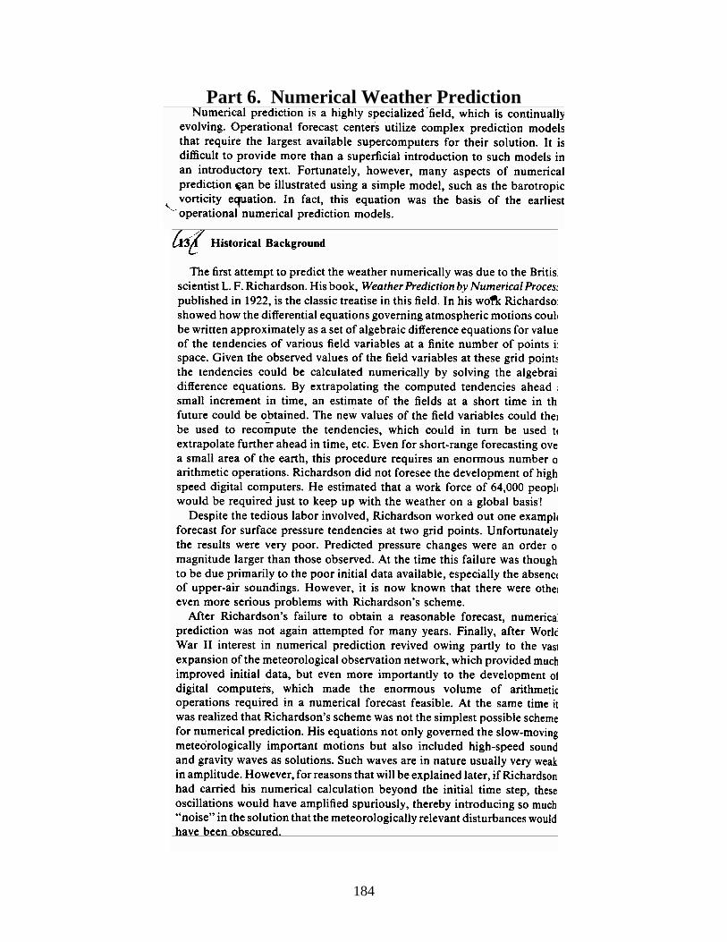
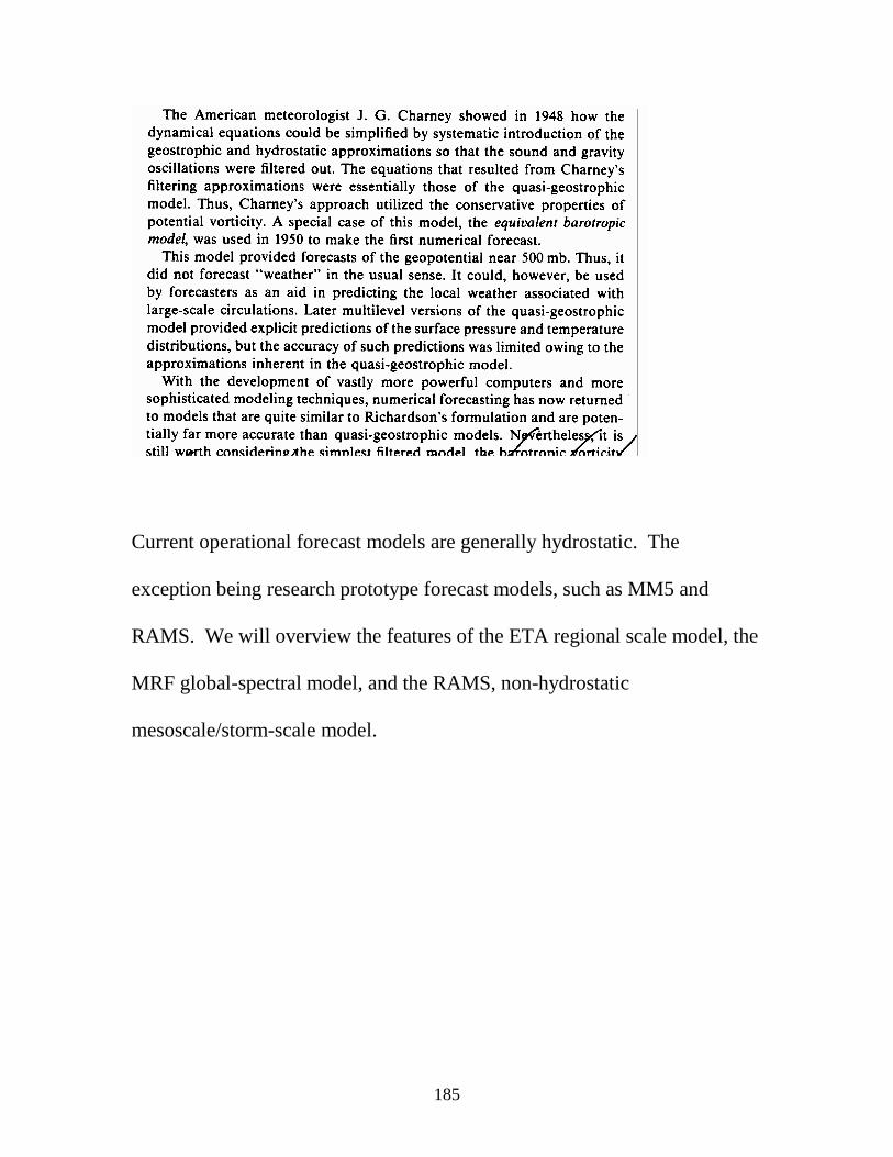
Part 6. Numerical Weather Prediction

185

Current operational forecast models are generally hydrostatic. The

exception being research prototype forecast models, such as MM5 and

RAMS. We will overview the features of the ETA regional scale model, the

MRF global-spectral model, and the RAMS, non-hydrostatic

mesoscale/storm-scale model.

186

The MediumThe MediumThe MediumThe Medium----Range Forecast Model Range Forecast Model Range Forecast Model Range Forecast Model status as of January 09, 2001

Model Documentation: Comprehensive documentation of the 1988 version of

the model was provided by the NMC (now NCEP) Development Division (1988),

with subsequent model development summarized by Kanamitsu(1989),

Kanamitsu et al. (1991), Kalnay et al. (1990).

The documentation NCEP MRF/RSM physics status as of August 1999 is located

here This document containing radiation, surface layer, vertical diffusion, gravity

wave drag, convective precipitation, shallow convection, non-convective

precipitation and references updates the old 1988 documentation. In addition

Office Note 424, New Global Orography Data Sets contains documentaiton of the

higher resolution orography for the MRF.

• Numerical/Computational Properties

o Horizontal RepresentationHorizontal RepresentationHorizontal RepresentationHorizontal Representation

Spectral (spherical harmonic basis functions) with transformation to

a Gaussian grid for calculation of nonlinear quantities and physics.

o Horizontal ResolutionHorizontal ResolutionHorizontal ResolutionHorizontal Resolution

Spectral triangular 170 (T170); Gaussian grid of 512x256, roughly equivalent to 0.7 X 0.7 degree latitude/longitude.

o Vertical DomainVertical DomainVertical DomainVertical Domain

Surface to about 2.0 hPa divided into 42 layers. For a surface pressure of 1000 hPa, the lowest atmospheric level is at a pressure of about 996 hPa.

o Vertical RepresentationVertical RepresentationVertical RepresentationVertical Representation

187

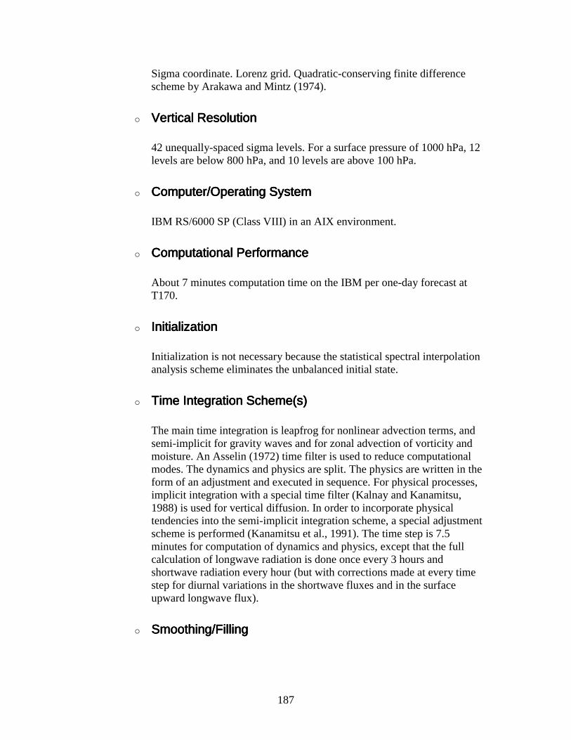
Sigma coordinate. Lorenz grid. Quadratic-conserving finite difference scheme by Arakawa and Mintz (1974).

o Vertical ResolutionVertical ResolutionVertical ResolutionVertical Resolution

42 unequally-spaced sigma levels. For a surface pressure of 1000 hPa, 12 levels are below 800 hPa, and 10 levels are above 100 hPa.

o Computer/Operating SystemComputer/Operating SystemComputer/Operating SystemComputer/Operating System

IBM RS/6000 SP (Class VIII) in an AIX environment.

o Computational PerformanceComputational PerformanceComputational PerformanceComputational Performance

About 7 minutes computation time on the IBM per one-day forecast at T170.

o InitializationInitializationInitializationInitialization

Initialization is not necessary because the statistical spectral interpolation analysis scheme eliminates the unbalanced initial state.

o Time Integration Scheme(s)Time Integration Scheme(s)Time Integration Scheme(s)Time Integration Scheme(s)

The main time integration is leapfrog for nonlinear advection terms, and semi-implicit for gravity waves and for zonal advection of vorticity and moisture. An Asselin (1972) time filter is used to reduce computational modes. The dynamics and physics are split. The physics are written in the form of an adjustment and executed in sequence. For physical processes, implicit integration with a special time filter (Kalnay and Kanamitsu, 1988) is used for vertical diffusion. In order to incorporate physical tendencies into the semi-implicit integration scheme, a special adjustment scheme is performed (Kanamitsu et al., 1991). The time step is 7.5 minutes for computation of dynamics and physics, except that the full calculation of longwave radiation is done once every 3 hours and shortwave radiation every hour (but with corrections made at every time step for diurnal variations in the shortwave fluxes and in the surface upward longwave flux).

o Smoothing/FillingSmoothing/FillingSmoothing/FillingSmoothing/Filling

188

Mean orographic heights on the Gaussian grid are used (see Orography). Negative atmospheric moisture values are not filled for moisture conservation, except for a temporary moisture filling that is applied in the radiation calculation.

• Dynamical/Physical Properties

o Atmospheric DynamicsAtmospheric DynamicsAtmospheric DynamicsAtmospheric Dynamics

Primitive equations with vorticity, divergence, logarithm of surface

pressure, specific humidityn and virtual temperature as dependent

variables.

o Horizontal DiffusionHorizontal DiffusionHorizontal DiffusionHorizontal Diffusion

Scale-selective, second-order horizontal diffusion after Leith (1971) is applied to vorticity, divergence, virtual temperature, and specific humidity. The diffusion of temperature and specific humidity are performed on quasi-constant pressure surfaces (Kanamitsu et al. 1991).

o Vertical DiffusionVertical DiffusionVertical DiffusionVertical Diffusion

See Planetary Boundary Layer

o GravityGravityGravityGravity----wave Dragwave Dragwave Dragwave Drag

Gravity-wave drag is simulated as described by Alpert et al. (1988). The parameterization includes determination of the momentum flux due to gravity waves at the surface, as well as at higher levels. The surface stress is a nonlinear function of the surface wind speed and the local Froude number, following Pierrehumbert (1987). Vertical variations in the momentum flux occur when the local Richardson number is less than 0.25 (the stress vanishes), or when wave breaking occurs (local Froude number becomes critical); in the latter case, the momentum flux is reduced according to the Lindzen (1981) wave saturation hypothesis. Modifications are made to avoid instability when the critical layer is near the surface, since the time scale for gravity-wave drag is shorter than the model time step (see also Time Integration Schemes and Orography). The treatment of the gravity-wave drag parameterization in the lower troposphere is improved by the use of the Kim and Arakawa (1995) enhancement. Included is a dependence of variance on wind direction relative to the mountain as well as subgrid statisical details of mountain

189

distribution. This improves the prediction of lee cyclogenesis and the accompanying movement of cold outbreaks (Alpert,et al, 199x).

o RadiationRadiationRadiationRadiation

Shortwave radiation is computed using multi-band techniques and includes absorption/scattering by water vapor, ozone, carbon dioxide, and clouds, with future options available for aerosols and oxygen. It is based on work by Chou (1992), Chou and Lee (1996), Chou (1990), and Hou, et al (1996). Data for Rayleigh scattering are calculated from Frohlich and Shaw's formulation (1980). Multi-scattering in clouds is treated using a delta-Eddington approximation with a two-stream adding method (Coakley, etal. 1983). Horizontal distribution of surface albedo is a function of Matthews (1985) surface vegetation types in a manner similar to Briegleb, etal (1986). Monthly variation of surface albedo is derived in reference to Staylor and Wilbur (1990). Longwave radiation follows the simplified exchange method of Fels and Schwarzkopf (1975) and Schwarzkopf and Fels (1991), with calculation over spectral bands associated with carbon dioxide, water vapor, and ozone. Schwarzkopf and Fels (1985) transmission coefficients for carbon dioxide, a Roberts et al. (1976) water vapor continuum, and the effects of water vapor-carbon dioxide overlap and of a Voigt line-shape correction are included. The Rodgers (1968) formulation is adopted for ozone absorption. Cloud radiative properties for shortwave (reflectance, absorptance) and longwave (emissivity) are obtained from cloud thickness, cloud layer temperature, and cloud layer moisture in a manner similar to Hashvardhan, Randall, Corsetti and Dazlich (1989). Independent cloud layered masses (separated by one clear layer) are randomly overlapped in the vertical direction. Vertically contiguous anvil cirrus and lower convective cloud is also randomly overlapped. See also Cloud Formulation.

o ConvectionConvectionConvectionConvection

Penetrative convection is simulated following Pan and Wu (1994), which is based on Arakawa and Schubert(1974) as simplified by Grell (1993) and with a saturated downdraft. Convection occurs when the cloud work function exceeds a certain threshold. Mass flux of the cloud is determined using a quasi-equilibrium assumption based on this threshold cloud work function. The cloud work function is a function of temperature and moisture in each air column of the model gridpoint. The temperature and moisture profiles are adjusted towards the equilibrium cloud function within a specified time scale using the deduced mass flux. A major simplification of the original Arakawa-Shubert scheme is to consider only the deepest cloud and not the spectrum of clouds. The cloud model incorporates a downdraft mechanism as well as the evaporation of

190

precipitation. Entrainment of the updraft and detrainment of the downdraft in the sub-cloud layers are included. Downdraft strenght is based on the vertical wind shear through the cloud. The critical cloud work function is a function of the cloud base vertical motion. As the large-scale rising motion becomes strong, the cloud work function (similar to CAPE) is allowed to approach zero (therefore approaching neutral stability).

o Shallow convectionShallow convectionShallow convectionShallow convection

Following Tiedtke (1983), the simulation of shallow (nonprecipitating) convection is parameterized as an extension of the vertical diffusion scheme. The shallow convection occurs where convective instability exist but no convection occurs. The cloud base is determined from the lifting condensation level and the vertical diffusion is invoked between the cloud top and the bottom. A fixed profile of vertical diffusion coefficients is assigned for the mixing process.

o Cloud FormationCloud FormationCloud FormationCloud Formation

The formation of stratiform clouds associated with fronts and tropical disturbances follows Slingo (1987) and Campana, et al (1994). Clouds are permitted to exist in most model layers (exceptions near the earth's surface and above the model-estimated tropopause). Stratiform cloud is computed from 10-month (March-December 1995) mean cloud/relative humidity relationships (Mitchell and Hahn, 1989), developed from U.S.A.F. RT Nephanalysis data, for tropics, mid-latitudes, land, sea, and vertical (high, middle, low, and 'boundary layer') regions. For the radiation computation, vertically contiguous diagnosed-cloud layers are maximally overlapped into individual cloud masses. The height of sub-gridscale convective cloud is determined by the level of non-buoyancy for moist adiabatic ascent (see Convection). The convective cloud fraction is a function of precipitation rate (Slingo, 1987). The fractional value of cloud cover is Slingo's convective coverage algorithm and the cloud is considered one columnar mass for the radiation calculations. Anvil cirrus also forms in the layer above the top of convection if precipitation is intense enough! See also Radiation for cloud-radiative interactions.

o PrecipitationPrecipitationPrecipitationPrecipitation

Precipitation is produced both from large-scale condensation and from the convective scheme (see Convection). The large-scale precipitation algorithm checks supersaturation in the predicted specific humidity, and latent heat is released to adjust the specific humidity and temperature to saturation. Evaporation of rain in the unsaturated layers below the level of

191

condensation is also taken into account. All precipitation that penetrates the bottom atmospheric layer is allowed to fall to the surface (see also Snow Cover). As of July 1998, a convective adjustment is included when the model column becomes super-saturated and conditionally unstable. The lowest level where supersaturation occurs is the cloud base and the cloud top is chosen as the maximum level where the theta-e from cloud base is warmer and while the resulting column can remain saturated.

o Planetary Boundary LayerPlanetary Boundary LayerPlanetary Boundary LayerPlanetary Boundary Layer

A new scheme based on the Troen and Mahrt (1986) paper was implemented on 25 October, 1995. The scheme is still a first-order vertical diffusion scheme. There is a diagnostically determined pbl height that uses the bulk-Richardson approach to iteratively estimate a pbl height starting from the ground upward. Once the pbl height is determined, the profile of the coefficient of diffusivity is specified as a cubic function of the pbl height. The actual values of the coefficients are determined by matching with the surface-layer fluxes. There is also a counter-gradient flux parameterization that is based on the fluxes at the surface and the convective velocity scale. (See Hong and Pan(1996) for a description of the scheme as well as a description of the convection scheme in the model).

o OrographyOrographyOrographyOrography

Raw orography obtained from the U.S. Navy dataset with resolution of 10 minutes arc (Joseph 1980) is area-averaged on the T126 Gaussian grid of the NMC operational model. Orographic variances are computed from the 10-minute dataset and also area-averaged to T126 Gaussian grid for use in the gravity-wave drag parameterization (see Gravity-wave Drag).

o OceanOceanOceanOcean

A 5-day running mean sea surface temperature analysis is used. The analysis is available once a day at 00GMT.

o Sea IceSea IceSea IceSea Ice

Sea-ice is obtained from the analysis by the marine Modeling Branch, available daily. The sea ice is assumed to have a constant thickness of 3 meters, and the ocean temperature below the ice is specified to be 271.2 K. The surface temperature of sea ice is determined from an energy balance that includes the surface heat fluxes (see Surface Fluxes) and the heat

192

capacity of the ice. Snow accumulation does not affect the albedo or the heat capacity of the ice.

o Snow CoverSnow CoverSnow CoverSnow Cover

Snow cover is obtained from an analysis by NESDIS (the IMS system) and the Air Force, updated daily. When the snow cover analysis is not available, the predicted snow in the data assimilation is used. Precipitation falls as snow if the temperature at sigma=.85 is below 0 C. Snow mass is determined prognostically from a budget equation that accounts for accumulation and melting. Snow melt contributes to soil moisture, and sublimation of snow to surface evaporation. Snow cover affects the surface albedo and heat transfer/capacity of the soil, but not of sea ice. See also Sea Ice, Surface Characteristics, Surface Fluxes, and Land Surface Processes.

o Surface CharacteristicsSurface CharacteristicsSurface CharacteristicsSurface Characteristics

Roughness lengths over oceans are determined from the surface wind stress after the method of Charnock (1955). Over sea ice the roughness is a uniform 0.01 cm. Roughness lengths over land are prescribed from data of Dorman and Sellers (1989) which include 12 vegetation types. Note that the surface roughness is not a function of orography. Over oceans the surface albedo depends on zenith angle. The albedo of sea ice is a function of surface skin temperature and nearby atmospheric temperature as well as snow cover (Grumbine, 1994), with values ranging from 0.65-0.8 for snow-covered sea ice and from 0.45-0.65 for bare sea ice. Albedoes for land surfaces are based on Matthews (1985) surface vegetation distribution (See Radiation). Longwave emissivity is prescribed to be unity (black body emission) for all surfaces. Soil type and Vegetation type data base from GCIP is used. Vegetation fraction monthly climatology based on NESDIS NDVI 5-year climatology is used.

o Surface Fluxes Surface Fluxes Surface Fluxes Surface Fluxes

Surface solar absorption is determined from the surface albedos, and longwave emission from the Planck equation with emissivity of 1.0 (see Surface Characteristics). The lowest model layer is assumed to be the surface layer (sigma=0.996) and the Monin-Obukhov similarity profile relationship is applied to obtain the surface stress and sensible and latent heat fluxes. The formulation was based on Miyakoda and Sirutis (1986) and has been modified by P. Long in the very stable and very unstable situations. A bulk aerodynamic formula is used to calculate the fluxes once the turbulent exchange coefficients have be obtained. Roughness

193

length over ocean is updated with a Charnock formula after surface stress has been obtained. Thermal roughness over the ocean is based on a formulation derived from TOGA COARE(Zeng et al, 1998). Land surface evaporation is comprised of three components: direct evaporation from the soil and from the canopy, and transpiration from the vegetation. The formulation follows Pan and Mahrt (1987).

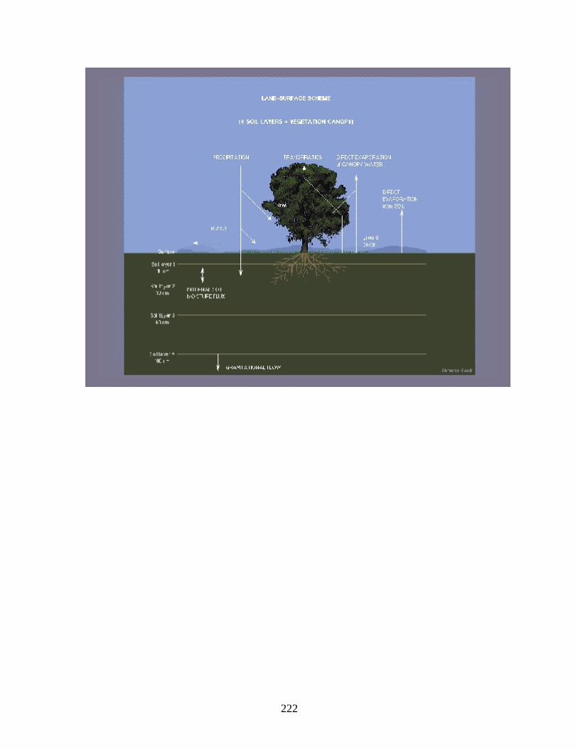
o Land Surface ProcessesLand Surface ProcessesLand Surface ProcessesLand Surface Processes

Soil temperature and soil volumetric water content are computed in two layers at depths 0.1 and 1.0 meters by a fully implicit time integration scheme (Pan and Mahrt, 1987). For sea ice, the layer depths were specified as 1.5 and 3 meters. Heat capacity, thermal and hydraulic diffusivity and hydraulic conductivity coefficients are strong functions of the soil moisture content. A climatological deep-soil temperature is specified at the third layer of 4 meters for soil and a constant value of 272 K is specified as the ice-water interface temperature for sea ice. The vegetation canopy is allowed to intercept precipitation and re-evaporation. Runoff from the surface and drainage from the bottom layer are also calculated.

o ChemistryChemistryChemistryChemistry

Ozone is now a prognostic variable that is updated in the analysis and transported in the model with zonally averaged seasonally varying sources and sinks. For longterm forecasts, we use a monthly zonal mean climatology obtained from NASA-Goddard.

ReferencesReferencesReferencesReferences

Alpert, J.C., S-Y Hong and Y-J Kim, 199x: Sensitivity of cyclogenesis to lower

troposphere enhancement of gravity wave drag using the Environmental

Modeling Center medium range model. REF Alpert, J.C., M. Kanamitsu, P.M.

Caplan, J.G. Sela, G.H. White, and E. Kalnay, 1988: Mountain induced gravity

wave drag parameterization in the NMC medium-range model. Preprints of the

Eighth Conference on Numerical Weather Prediction, Baltimore, MD, American

Meteorological Society, 726-733.

Arakawa, A. and W. H. Shubert, 1974: Interaction of a Cumulus Ensemble with

the Large-Scale Environment, Part I. J. Atmos. Sci., 31, 674-704.

194

Asselin, R., 1972: Frequency filter for time integrations. Mon. Wea. Rev., 100,

487-490.

Betts, A.K., S.-Y. Hong and H.-L. Pan, 1996: Comparison of NCEP-NCAR

Reanalysis with 1987 FIFE data. Mon. Wea. Rev., 124, 1480-1498

Briegleb, B. P., P. Minnus, V. Ramanathan, and E. Harrison, 1986: Comparison

of regional clear-sky albedo inferred from satellite observations and model

computations. J. Clim. and Appl. Meteo., 25, 214-226.

Campana, K. A., Y-T Hou, K. E. Mitchell, S-K Yang, and R. Cullather, 1994:

Improved diagnostic cloud parameterization in NMC's global model. Preprints of

the Tenth Conference on Numerical Weather Prediction, Portland, OR, American

Meteorological Society, 324-325.

Charnock, H., 1955: Wind stress on a water surface. Quart. J. Roy. Meteor. Soc.,

81, 639-640.

Chen, F., K. Mitchell, J. Schaake, Y. Xue, H.-L. Pan, V. Koren, Q. Y. Duan, M.

Ek, and A. Betts, 1996: Modeling of land surface evaporation by four schemes

and comparison with FIFE observations. J. Geophys. Res., 101, D3, 7251-7268.

Chou, M-D, 1990: Parameterizations for the absorption of solar radiation by O2

and CO2 with application to climate studies. J. Climate, 3, 209-217.

Chou, M-D, 1992: A solar radiation model for use in climate studies. J. Atmos.

Sci., 49, 762-772.

Chou, M-D and K-T Lee, 1996: Parameterizations for the absorption of solar

radiation by water vapor and ozone. J. Atmos. Sci., 53, 1204-1208.

Coakley, J. A., R. D. Cess, and F. B. Yurevich, 1983: The effect of tropospheric

aerosols on the earth's radiation budget: a parameterization for climate models.

J. Atmos. Sci., 42, 1408-1429.

Dorman, J.L., and P.J. Sellers, 1989: A global climatology of albedo, roughness

length and stomatal resistance for atmospheric general circulation models as

represented by the Simple Biosphere model (SiB). J. Appl. Meteor., 28, 833-855.

Fels, S.B., and M.D. Schwarzkopf, 1975: The simplified exchange approximation:

A new method for radiative transfer calculations. J. Atmos. Sci., 37, 2265-2297.

195

Frohlich, C. and G. E. Shaw, 1980: New determination of Rayleigh scattering in

the terrestrial atmosphere. Appl. Opt., 14, 1773-1775.

Grell, G. A., 1993: Prognostic Evaluation of Assumprions Used by Cumulus

Parameterizations. Mon. Wea. Rev., 121, 764-787.

Grumbine, R. W., 1994: A sea-ice albedo experiment with the NMC medium

range forecast model. Weather and Forecasting, 9, 453-456.

Harshvardhan, D. A. Randall, T. G. Corsetti and D. A. Dazlich, 1989: Earth

radiation budget and cloudiness simulation with a general circulation model. J.

Atmos. Sci., 46, 1922-1942.

Hong, S.-Y. and H.-L. Pan, 1996: Nonlocal boundary layer vertical diffusion in a

medium-range forecast model. Mon. Wea. Rev., 124, 2322-2339.

Hou, Y-T, K. A. Campana and S-K Yang, 1996: Shortwave radiation calculations

in the NCEP's global model. International Radiation Symposium, IRS-96, August

19-24, Fairbanks, AL.

Joseph, D., 1980: Navy 10' global elevation values. National Center for

Atmospheric Research notes on the FNWC terrain data set, 3 pp.

Kalnay, E. and M. Kanamitsu, 1988: Time Scheme for Stronglyt Nonlinear

Damping Equations. Mon. Wea. Rev., 116, 1945-1958.

Kalnay, M. Kanamitsu, and W.E. Baker, 1990: Global numerical weather

prediction at the National Meteorological Center. Bull. Amer. Meteor. Soc., 71,

1410-1428.

Kanamitsu, M., 1989: Description of the NMC global data assimilation and

forecast system. Wea. and Forecasting, 4, 335-342.

Kanamitsu, M., J.C. Alpert, K.A. Campana, P.M. Caplan, D.G. Deaven, M.

Iredell, B. Katz, H.-L. Pan, J. Sela, and G.H. White, 1991: Recent changes

implemented into the global forecast system at NMC. Wea. and Forecasting, 6,

425-435.

Kim, Y-J and A. Arakawa, 1995: Improvement of orographic gravity wave

parameterization using a mesoscale gravity wave model. J. Atmos. Sci. 52, 11,

1875-1902.

196

Lacis, A.A., and J. E. Hansen, 1974: A parameterization for the absorption of

solar radiation in the Earth's atmosphere. J. Atmos. Sci., 31, 118-133.

Leith, C.E., 1971: Atmospheric predictability and two-dimensional turbulence. J.

Atmos. Sci., 28, 145-161.

Lindzen, R.S., 1981: Turbulence and stress due to gravity wave and tidal

breakdown. J. Geophys. Res., 86, 9707-9714.

Matthews, E., 1985: "Atlas of Archived Vegetation, Land Use, and Seasonal

Albedo Data Sets.", NASA Technical Memorandum 86199, Goddard Institute for

Space Studies, New York.

Mitchell, K. E. and D. C. Hahn, 1989: Development of a cloud forecast scheme

for the GL baseline global spectral model. GL-TR-89-0343, Geophysics

Laboratory, Hanscom AFB, MA.

Miyakoda, K., and J. Sirutis, 1986: Manual of the E-physics. [Available from

Geophysical Fluid Dynamics Laboratory, Princeton University, P.O. Box 308,

Princeton, NJ 08542.]

NMC Development Division, 1988: Documentation of the research version of the

NMC Medium-Range Forecasting Model. NMC Development Division, Camp

Springs, MD, 504 pp.

Pan, H-L. and L. Mahrt, 1987: Interaction between soil hydrology and boundary

layer developments. Boundary Layer Meteor., 38, 185-202.

Pan, H.-L. and W.-S. Wu, 1995: Implementing a Mass Flux Convection

Parameterization Package for the NMC Medium-Range Forecast Model. NMC

Office Note, No. 409, 40pp. [ Available from NCEP, 5200 Auth Road,

Washington, DC 20233 ]

Pierrehumbert, R.T., 1987: An essay on the parameterization of orographic wave

drag. Observation, Theory, and Modelling of Orographic Effects, Vol. 1, Dec.

1986, European Centre for Medium Range Weather Forecasts, Reading, UK,

251-282.

Ramsay, B.H., 1998: The interactive multisensor snow and ice mapping system.

Hydrol. Process. 12, 1537-1546.

197

Roberts, R.E., J.A. Selby, and L.M. Biberman, 1976: Infrared continuum

absorption by atmospheric water vapor in the 8-12 micron window. Appl. Optics.,

15, 2085-2090.

Rodgers, C.D., 1968: Some extension and applications of the new random model

for molecular band transmission. Quart. J. Roy. Meteor. Soc., 94, 99-102.

Schwarzkopf, M.D., and S.B. Fels, 1985: Improvements to the algorithm for

computing CO2 transmissivities and cooling rates. J. Geophys. Res., 90, 10541-

10550.

Schwarzkopf, M.D., and S.B. Fels, 1991: The simplified exchange method

revisited: An accurate, rapid method for computation of infrared cooling rates and

fluxes. J. Geophys. Res., 96, 9075-9096.

Sela, J., 1980: Spectral modeling at the National Meteorological Center, Mon.

Wea. Rev., 108, 1279-1292.

Slingo, J.M., 1987: The development and verification of a cloud prediction model

for the ECMWF model. Quart. J. Roy. Meteor. Soc., 113, 899-927.

Staylor, W. F. and A. C. Wilbur, 1990: Global surface albedoes estimated from

ERBE data. Preprints of the Seventh Conference on Atmospheric Radiation, San

Francisco CA, American Meteorological Society, 231-236.

Tiedtke, M., 1983: The sensitivity of the time-mean large-scale flow to cumulus

convection in the ECMWF model. ECMWF Workshop on Convection in Large-

Scale Models, 28 November-1 December 1983, Reading, England, pp. 297-316.

Troen, I. and L. Mahrt, 1986: A simple model of the atmospheric boundary layer;

Sensitivity to surface evaporation. Bound.-Layer Meteor., 37, 129-148

Zeng, X., M. Zhao, and R.E. Dickinson, 1998: Intercomparison of bulk

aerodynamical algorithms for the computation of sea surface fluxes using TOGA

COARE and TAO data. J. Climate, 11, 2628-2644.

This web site and sites that are part of the EMC distributed Web operate under

the NWS Web policy - click here

for Disclaimer click here

198

199

200

201

202

203

204

205

206

207

208

209

210

211

212

213

214

215

216

217

218

219

220

221

222

223

224

225

226

227

228

229

230

231

232

233

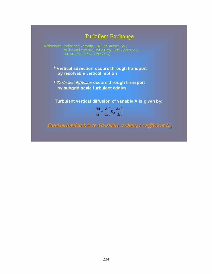
234

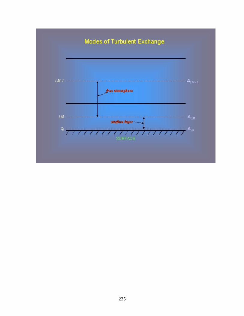
235

236

237

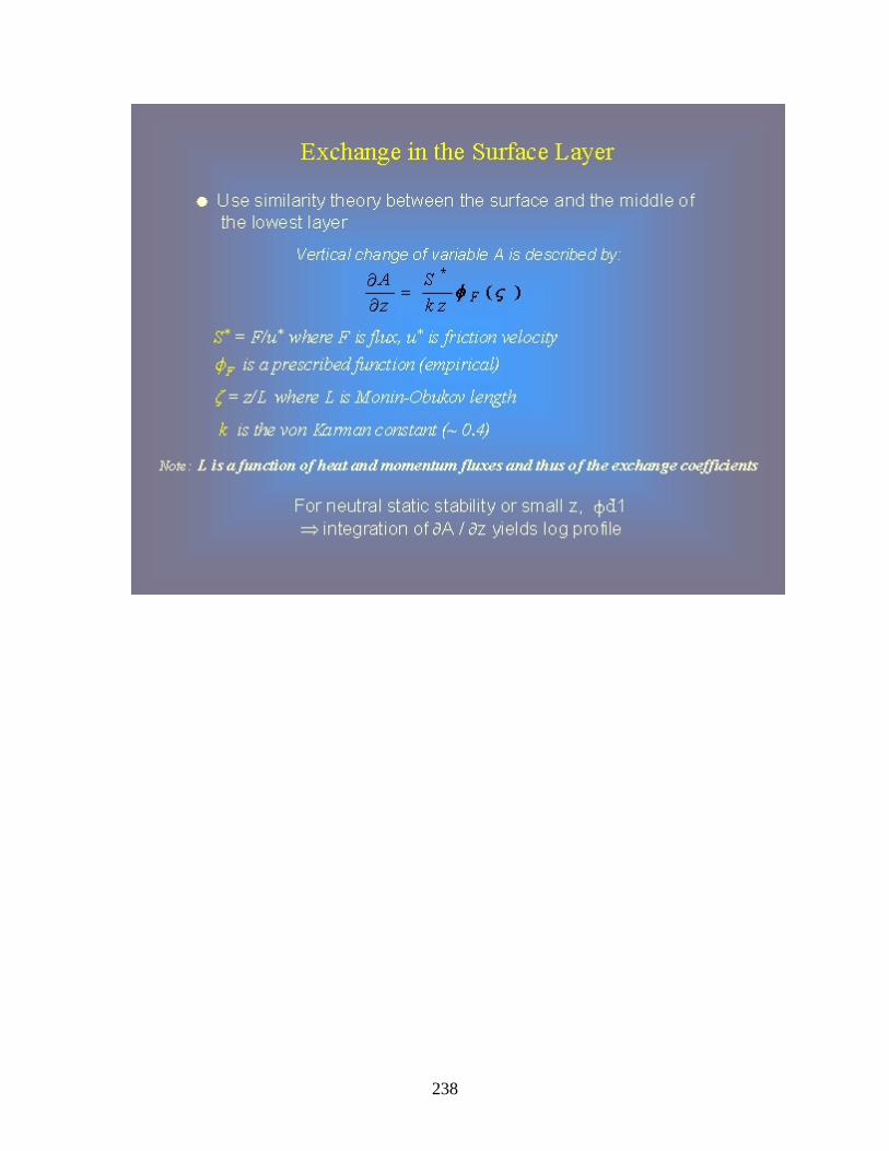
238

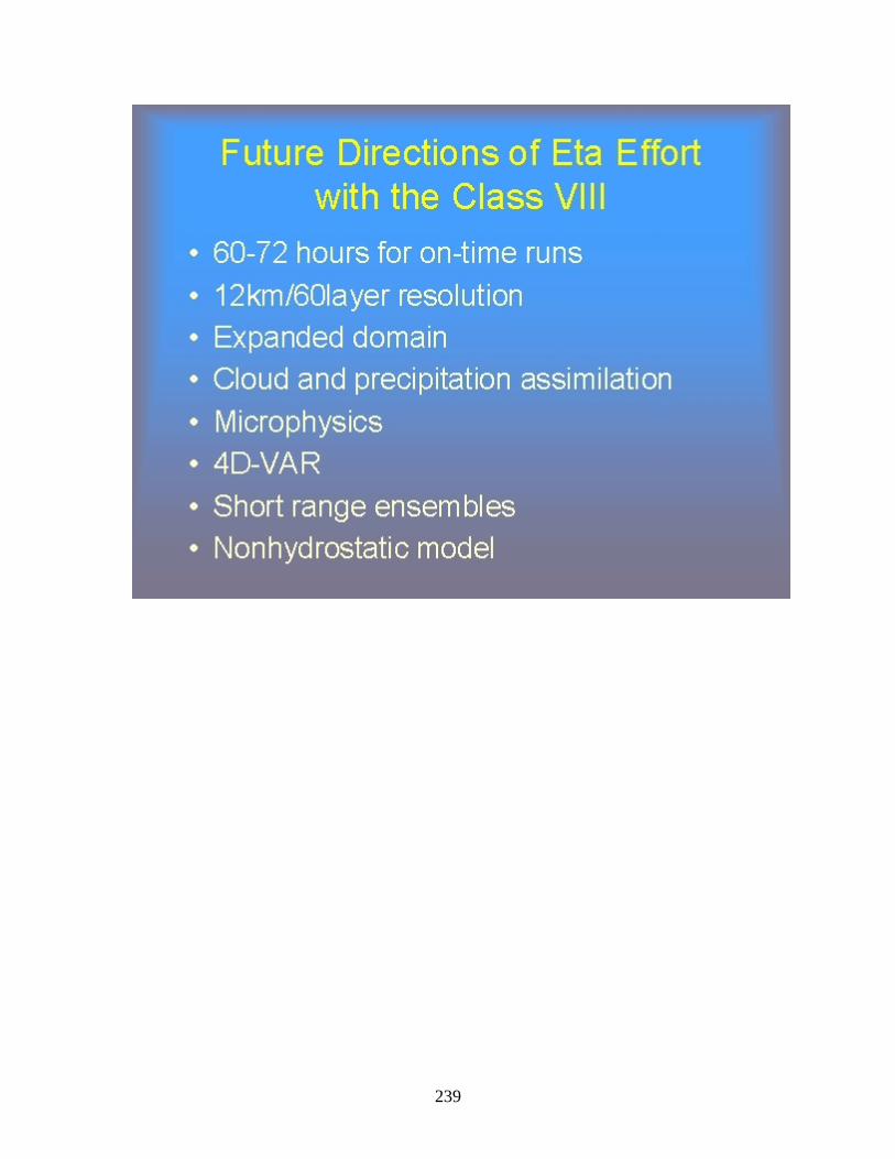
239

240

241

242

243

244

RAMS 2001: Current Status and Future Directions

1.0 Introduction

RAMS, which was developed at Colorado State University and MRC/*ASTeR, is a

multipurpose, numerical prediction model that simulates atmospheric circulations ranging

in scale from an entire hemisphere down to large eddy simulations (LES) of the planetary

boundary layer. It is most frequently used to simulate atmospheric phenomena on the

mesoscale (horizontal scales from 2 km to 2000 km) for applications ranging from

operational weather forecasting to air quality regulatory applications to support of basic

research. RAMS has often been successfully used with much higher resolutions to

simulate boundary layer eddies (10-100 m grid spacing), individual building simulation

(1 m grid spacing), and direct wind tunnel simulation (1 cm grid spacing). RAMS’

predecessor codes were developed to perform research in modeling physiographically

driven weather systems and simulating convective clouds, mesoscale convective systems,

cirrus clouds, and precipitating weather systems in general. RAMS use has increased to

more than 120 current RAMS installations in more than 30 different countries.

The RAMS concept was created in the early 1980’s at Colorado State University by

merging three related models: the CSU cloud/mesoscale mode (Tripoli and Cotton,

1982), a hydrostatic version of the cloud model (Tremback, 1990), and the sea breeze

model described by Mahrer and Pielke (1977).

The original RAMS was run exclusively on the NCAR CRAY-1 machine. That

machine’s small central memory (1 Mword or 8 Mbytes) forced various design constructs

that limited its application to what we would consider today to be small runs. When

computers with significantly more memory became available the entire RAMS code was

245

rewritten, obsolete features were removed, and parameterizations from the sea breeze

model were included. The first version of the “new” RAMS was released in 1988 as

version 0a, and the first widely distributed version, version 2c, was released in 1991.

A key issue in RAMS development was taking full advantage of modern parallel

computer capabilities. RAMS first parallel version was developed at CSU in 1991.

Message Passing Interface (MPI) did not exist then, so Parallel Virtual Machine (PVM)

was used for the message-passing package. An essentially complete version was finished

in 1994, support for MPI was implemented in 1995, and a prototype operational version

of the parallel RAMS was installed at Kennedy Space Center in late 1995. RAMS is well

suited for parallelization since it does not use global physical/numerical routines. For

example, it calculates pressure locally and non-hydrostatically using a time-split

compressible approximation. Also, advection is calculated using local finite difference

operators rather than non-local spectral methods.

1.0 Summary of RAMS Options

The current released version of RAMS is designated as version 4.3. RAMS provides

a broad range of options that allow it to be tailored for a wide range of applications. The

code contains a variety of structures and features ranging from non-hydrostatic codes,

resolution ranging from less than a meter to a hundred kilometers, domains from a few

kilometers to the entire globe, and a suite of physical options. This allows users to easily

select appropriate options for different spatial scales, meteorological problems or

applications, or locations.

246

RAMS has a multiple grid nesting scheme that lets it solve the model equations

simultaneously on any number of interacting computational meshes of differing spatial

resolution. The highest resolution meshes are used to model details of small-scale

atmospheric systems, such as flow over complex terrain and surface-induced thermal

circulations. Coarse meshes are used to model the environment of these smaller systems

and provide boundary conditions for the fine mesh regions. Coarse meshes are also used

to simulate large scale atmospheric systems that interact with the smaller-scale systems

resolved on the finer grids.

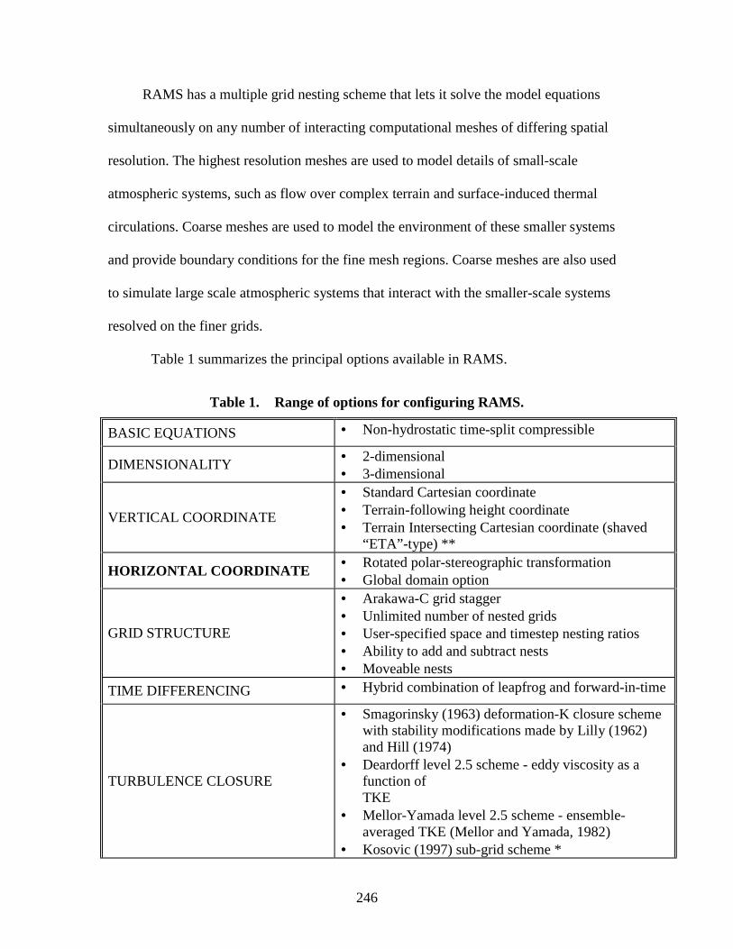
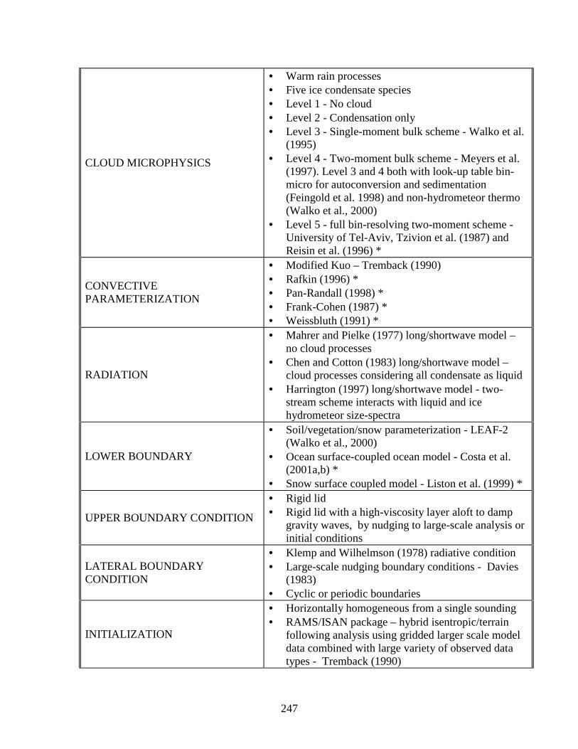
Table 1 summarizes the principal options available in RAMS.

Table 1. Range of options for configuring RAMS.

BASIC EQUATIONS • Non-hydrostatic time-split compressible

DIMENSIONALITY • 2-dimensional • 3-dimensional

VERTICAL COORDINATE

• Standard Cartesian coordinate • Terrain-following height coordinate • Terrain Intersecting Cartesian coordinate (shaved

“ETA”-type) **

HORIZONTAL COORDINATE • Rotated polar-stereographic transformation • Global domain option

GRID STRUCTURE

• Arakawa-C grid stagger • Unlimited number of nested grids • User-specified space and timestep nesting ratios • Ability to add and subtract nests • Moveable nests

TIME DIFFERENCING • Hybrid combination of leapfrog and forward-in-time

TURBULENCE CLOSURE

• Smagorinsky (1963) deformation-K closure scheme with stability modifications made by Lilly (1962) and Hill (1974)

• Deardorff level 2.5 scheme - eddy viscosity as a function of TKE

• Mellor-Yamada level 2.5 scheme - ensemble-averaged TKE (Mellor and Yamada, 1982)

• Kosovic (1997) sub-grid scheme *

247

CLOUD MICROPHYSICS

• Warm rain processes • Five ice condensate species • Level 1 - No cloud • Level 2 - Condensation only • Level 3 - Single-moment bulk scheme - Walko et al.

(1995) • Level 4 - Two-moment bulk scheme - Meyers et al.

(1997). Level 3 and 4 both with look-up table bin-micro for autoconversion and sedimentation (Feingold et al. 1998) and non-hydrometeor thermo (Walko et al., 2000)

• Level 5 - full bin-resolving two-moment scheme - University of Tel-Aviv, Tzivion et al. (1987) and Reisin et al. (1996) *

CONVECTIVE PARAMETERIZATION

• Modified Kuo – Tremback (1990) • Rafkin (1996) * • Pan-Randall (1998) * • Frank-Cohen (1987) * • Weissbluth (1991) *

RADIATION

• Mahrer and Pielke (1977) long/shortwave model – no cloud processes

• Chen and Cotton (1983) long/shortwave model – cloud processes considering all condensate as liquid

• Harrington (1997) long/shortwave model - two-stream scheme interacts with liquid and ice hydrometeor size-spectra

LOWER BOUNDARY

• Soil/vegetation/snow parameterization - LEAF-2 (Walko et al., 2000)

• Ocean surface-coupled ocean model - Costa et al. (2001a,b) *

• Snow surface coupled model - Liston et al. (1999) *

UPPER BOUNDARY CONDITION

• Rigid lid • Rigid lid with a high-viscosity layer aloft to damp

gravity waves, by nudging to large-scale analysis or initial conditions

LATERAL BOUNDARY CONDITION

• Klemp and Wilhelmson (1978) radiative condition • Large-scale nudging boundary conditions - Davies

(1983) • Cyclic or periodic boundaries

INITIALIZATION

• Horizontally homogeneous from a single sounding • RAMS/ISAN package – hybrid isentropic/terrain

following analysis using gridded larger scale model data combined with large variety of observed data types - Tremback (1990)

248

DATA ASSIMILATION • Four-dimensional “analysis” nudging to data analyses

COMPUTER ASPECTS

• Operating systems: UNIX, LINUX, MS Windows 95/98/NT/2000

• Parallel processing on distributed and shared memory platforms using Message Passing Interface (MPI)

* option only in research versions at Colorado State University ** option under development

4.8 Prototype realtime forecasting with RAMS

At Colorado State University RAMS has been used for real-time forecasting since

1991 (Cotton et al., 1994; http://rams.atmos.colostate.edu/cases/). The feasibility of

using RAMS as a forecast model has been investigated also by Snook and Pielke (1995),

Mukabana and Pielke (1996), and Papineau et al. (1994). Originally a simple ‘dump-

bucket’ scheme (Cotton et al., 1995) was used to generate quantitative precipitation

forecasts (QPF), but starting in the fall of 1995 real-time forecasts used the bulk

microphysics scheme available with RAMS. Gaudet and Cotton (1998) showed that the

bulk microphysics improved the forecasting of the areal extent and maximum amount of

precipitation, especially when compared to the snow telemetry (SNOTEL) automatic

pillow-sensor stations, which are found at locations more representative of the model

topography. For the month of April 1995, a series of 24-hour accumulated precipitation

forecasts was generated with both the dump-bucket and microphysics versions of the

forecast model. Both sets of output were compared to a set of 167 community-based

station reports, and to a set of 32 SNOTEL stations. Climatological station precipitation

forecasts were improved on the average by correcting for the difference between a

station's actual elevation and the cell-averaged topography used by the model. The model

249

had more problems with the precise timing and geographical location of the precipitation

features, probably due in part to the influence of other model physics, the failure of the

model to resolve adequately winter-time convection events, and lack of mesoscale detail

in the initializations.

The current prototype realtime forecast version of RAMS at CSU is based on version

4.29. The model is set up on a 21-processor cluster of 450 MHz Pentium PCs. Two

configurations are run daily. The first is the standard meteorological forecast model

configuration that has three interactive nested grids. Grid #1 has 48 km grid spacing and

covers the entire U.S. (see Figure 4), Grid #2 has 12 km grid spacing and covers all of

Colorado, most of Wyoming, and portions of adjacent states, and Grid #3 has 3 km grid

spacing covering a 150 km x 150 km area that is relocatable anywhere within Grid #2.

Vertical grid spacing on all grids starts with 150-km spacing at the lowest levels and is

stretched to 1000m aloft, with a total of 36 vertical levels extending into the

stratosphere. The model is initialized with 00UTC ETA model analysis fields and run for

a period of 48h, with the lateral boundary region of the coarse grid nudged to the ETA 6-

hourly forecast fields. A 48h run takes about 4h of CPU. We are currently assessing the

value added to the forecasts using the 3 km grid. Preliminary analysis suggests that the

model is able to forecast the formation and propagation of individual convective storms,

especially those originating in the mountains, and severe downslope windstorm events

(see Cotton et al., 1995). The model exhibits a consistent over-prediction bias on

precipitation. We are currently seeking the source of that bias and hope to rectify that

shortly. Although “false alarms” of precipitation events are forecast, they occur relatively

rarely.

250

The second prototype forecast model emphasizes boundary layer forecast

applications. In this configuration Grid #1 is the same as the standard forecast model.

Grid #2 is similarly configured as well, except that it and Grid #3 can be relocated

anywhere in the continental U.S. Grid #3 has vertically nested levels with 50 m spacing

to 1 km and 75 m spacing to 1.5 km, and covers a 150 km x 150 km area with 3 km

horizontal spacing. This version is initialized with 1200 UTC ETA model analysis fields

and is also nudged to ETA forecast boundaries for a 48 h period. The aim of this forecast

cycle is to provide high-resolution, accurate forecasts of boundary layer winds,

temperature, moisture, turbulence (using the Mellor and Yamada (1974) level 2.5 TKE

scheme), and other specialized products. One such product we jokingly call the Cotton

Soaring Index (CSI), see Figure 5. This product is available on all RAMS forecast grids.

It uses model surface forecast temperatures and then calculates the difference between

forecast air temperatures 1600m above the local grid point ground level and the

temperature of a parcel lifted dry adiabatically to that level. Like the lifted index, the

more negative the value of CSI, the better the potential for finding good thermals for

soaring gliders. The height of 1600 m AGL is chosen because it is high enough above

ground level to permit safe cross-country flights in gliders. Other model products useful

to soaring forecasting are vertical cross sections of TKE (giving boundary layer

depth variablility over terrain), cloud base heights, winds, and precipitation. Relocatable

grid operations with this model have been tested over the Whitesands Missile Range, near

Littlefield, TX in support of a Soaring Society of America regional forecast contest,

Tucson, AR, to support Dr. Cotton's glider flights in the area, in the vicinity of the WLEF

Tower, WI in support of CO2 Budget and Rectification Airborne Study (COBRA) at

251

various locations in Colorado, southern Minnesota, and near Leon, Kansas in support of

the CASES-99 field experiment (see website:

http://www.colorado-research.com/cases/CASES-99.html). Detailed evaluations of the

boundary forecast model is underway using data acquired during CASES-99.

252

Cloud Microphysics and Weather Forecasting Current numerical prediction models have very crude cloud microphysics parameterizations, if they have any at all. Most have some variation on a Kessler-type scheme in which it is assumed that all precipitation elements have an exponential size-spectrum and that they all fall with a mass-weighted mean terminal velocity. Large hydrometeors collect smaller droplets by continuous accretion, and bulk evaporation rates for precipitation particles are estimated. The bulk microphysics is applied to the explicitly-resolved motions which in forecast models is represented by grid spacings of ten’s of kilometers. Unfortunately, the grid-resolved vertical motions are typically a few tenths of a meter per second while even for stratocumulus clouds actual cloud velocities are of the order of a meter per second. But this does not matter much since these parameterization schemes do not represent cloud nucleation processes anyway. Only the rate of sedimentation of hydrometeors is affected by the lack of cloud-scale vertical motions. Some research forecast models such as RAMS have more sophisticated microphysics algorithms. RAMS, for example, also uses a bulk microphysics model as the size-spectra of hydrometeors is specified to be a generalized gamma function. But, the physics includes such processes as stochastic collection of hydrometeors using look-up tables for computational efficiency. Moreover sedimentation of hydrometeors is done via look-up tables in which the hydrometeor spectra is broken up into bins to calculate sedimentation rates. Also, RAMS has the option of predicting on one or two moments of the size-spectra. When two moments are predicted, only the width parameter nu is user-specified. In most models using bulk microphysics, the initial broadening of the nucleated droplet spectra to drizzle-sized drops is parameterized with rather ad hoc autoconversion formulations. Others derive autoconversion rates from idealized box simulations in which the initial droplet concentration, size-spectra, and liquid water content is specified and then the autoconversion formula is fitted to the results of a sequence of simulations over the specified initial parameter space. A different procedure is adopted in RAMS. The generalized gamma distribution function is applied to cloud droplets having a size of a few micrometers to 100 micrometers. Then using realistic collection kernels, self-collection amongst cloud droplets is calculated with the aid of look-up tables to represent autoconversion. A

253

recent advance in RAMS microphysics is the addition of a second cloud-droplet mode covering the size-range of 40 to 80 micrometers. This is expected to provide greater skill in the simulation of initial broadening of droplets and permit the representation of processes such as nucleation on giant cloud condensation nuclei(GCCN) to form larger-mode droplets. Droplets in the large cloud droplet mode can participate in sedimentation, which can be important in fogs and stratus clouds and provide a better representation of Hallett-Mossop ice multiplication since it is dependent on a mix of large and small cloud droplets. Currently RAMS as well as other bulk microphysics models is initialized with a specified cloud droplet concentration. Now droplet concentrations are controlled by airmass properties(ie. Maritime, continental, polluted), and peak supersaturations in clouds. Peak supersaturations, in turn, are controlled by cloud dynamics such as vertical motions as well as airmass properties. For example, in a moderately clean continental airmass, droplet concentrations may reach 600/cc in cumulus clouds as peak supersaturations may be close to 1%, whereas stratus clouds in the same airmass may have concentrations less than 100/cc since peak supersaturations may not exceed 0.1%. Thus when modeling individual clouds, with a model such as RAMS, one can guess that if the clouds are cumulonimbi, and the airmass is clean continental, then droplet concentrations should be 600/cc. However, when one performs mesoscale or global forecasts, clouds of a variety of types and in all sorts of different airmasses can occur in a forecast cycle. It thus does not make sense to prescribe droplet concentrations. The next generation of RAMS will have the ability to predict the transport and dispersion and sources and sinks of CCN and GCCN. What needs to be done is to develop and objective methodology for characterizing airmasses with respect to CCN and GCCN concentrations. This will have to be rather crude since we do not have realtime observations of CCN/GCCN especially vertical soundings. It is not uncommon for an airmass with warm-frontal over-riding air, to exhibit, high CCN concentrations in the boundary layer, and be very clean aloft in the over-riding air, and with airmasses with very different trajectories with height, be dirty above that. Thus, stratus clouds can have large variations in droplet concentrations depending on airmass properties. Another thing we need to do is develop parameterizations of source functions of CCN/GCCN. Thus not only do we need to objectively initialize the model, but since there are sinks in CCN/GCCN, primarily do to nucleation, we also need to account for sources such as over urban areas versus over clean oceans.

254

I have mentioned earlier that mesoscale and general circulation NWP (or climate) models do not explicitly resolve cloud-scale vertical motions, which we have shown are important to predicting cloud droplet concentrations. One way of overcoming this deficiency is by using a cloud parameterization, which provides vertical velocity-scale information. An example is Chris Golaz’s boundary layer cloud model that provides a probability density function (pdf) of vertical velocity. Given that information, in principle (Chris is scheduled to do that in a postdoc appointment), one can then diagnose peak supersaturations and thus droplet concentrations. This approach would still have to be applied to non-boundary layer clouds and deep convective clouds. The approach of explicitly predicting of cloud-forming aerosol should also be done for ice forming nuclei (IFN). There is no reason to expect that IFN are horizontally and vertically uniform in concentrations. For many years in RAMS we have assumed that IFN concentrations fall off with height, much like the concentrations of large aerosol particles is known to decay. The basis of this parameterization is that there are limited observations, which suggest that IFN concentrations correlate with large aerosol concentrations. On the other hand, we have observations in the Arctic where IFN concentrations in the boundary layer are very low, but above the boundary layer inversion concentrations can be 100 times greater, but still be less than in most mid-latitude sites. The implication is that air originating in lower latitude industrial areas, is advected into the Arctic basin (with some cleansing by sedimentation and nucleation), and thereby contaminating the clouds. There are also observations, which suggest that some industries like heavy metal refining factories are excellent sources of IFN. In RAMS we have also developed the capability of predicting the advection and diffusion of IFN. The problem is that there is not sufficient data to guide us in developing simple algorithms for identifying airmass properties with regard to IFN concentrations or IFN source functions. What are the potential gains in having prognostic CCN/GCCN/IFN concentrations? We know that the efficiency of precipitation formation is related to the concentrations of these aerosols. Thus one would expect that if we can forecast their concentrations with some skill it would improve precipitation forecast skill. In addition, cloud fractional coverage, is influenced by the precipitation efficiency of clouds. Heavily precipitating clouds will in general exhibit lower cloud coverage, which will influence

255

solar heating rates at the ground in particular, and longwave radiation cooling rates. Thus forecasting these aerosols and their variability would be of benefit to not only short-and medium-range prediction, but also to climate forecasting/simulations. Another application area is aircraft icing prediction. Aircraft icing is not only a function of the amount of supercooled water in clouds, but also the size-spectrum of drops. Thus a cloud containing moderate amounts of liquid water, all on very small droplets, would have little aircraft icing potential while the same clouds containing large cloud droplets and drizzle drops might have severe icing potential. Forecasting the broadness of droplet spectra is thereby important to aircraft icing prediction. But, the amount of supercooled water in a cloud is the residual between production of liquid water by condensation and removal of water by precipitation and growth of ice particles. Thus icing prediction is dependent upon forecasts of both ice crystal concentrations and sizes (i.e., IFN concentrations) and on CCN/GCCN concentrations. Are the benefits worth the added expense? The costs are non-trivial, but I estimate that we could forecast CCN/GCCN/IFN concentrations and their activation, sources and sinks, etc by expanding our current cluster of twenty-one 450 Mhz PCs having 128 MB ROM per processor, to twenty-one 1 Ghz PC with 1GB ROM per processor for a cost of $21,000. This is not a big investment if we could demonstrate that with that forecasting ability, we could improve the forecasts of precipitation, cloud cover, icing, etc substantially. We have to try it to see if the costs are worth the expenses.