Embed Size (px)
DESCRIPTION
대기과학에서의 수치모델링 (Numerical Weather Prediction, NWP). 홍 성 유 연세대학교. 순서. 수치예보에 대한 개념 및 역사 수치 모형의 구성 WRF 모형의 특성 예측도 한계. 홍성유 ( 연세대 ). 현업 모델 개발 경력. 관련 논문 : 국내 (15), 국제 SCI (34). 한국형 전산예보 시스템 개발 ( 서울대 , 1986-1989). 미국 기상청 현업모델의 개발 (NCEP/EMC, 1993-2000). - PowerPoint PPT Presentation
Citation preview
Numerical Modeling Laboratory
Numerical Modeling Laboratory
Yonsei UniversityYonsei University
홍 성 유연세대학교
홍 성 유연세대학교
대기과학에서의 수치모델링(Numerical Weather
Prediction, NWP)
대기과학에서의 수치모델링(Numerical Weather
Prediction, NWP)

Numerical Modeling Laboratory
Numerical Modeling Laboratory
Yonsei UniversityYonsei University
•수치예보에 대한 개념 및 역사
•수치 모형의 구성
•WRF 모형의 특성
•예측도 한계
•수치예보에 대한 개념 및 역사
•수치 모형의 구성
•WRF 모형의 특성
•예측도 한계
순서순서

Numerical Modeling Laboratory
Numerical Modeling Laboratory
Yonsei UniversityYonsei University
홍성유 홍성유 (( 연세대연세대 ))
한국형 전산예보 시스템 개발 ( 서울대 , 1986-1989)한국형 전산예보 시스템 개발 ( 서울대 , 1986-1989)
현업 모델 개발 경력현업 모델 개발 경력
미국 기상청 현업모델의 개발 (NCEP/EMC, 1993-2000)미국 기상청 현업모델의 개발 (NCEP/EMC, 1993-2000)
적운모수화 (Hong and Pan 1998, MWR) : 1998 년 현업구름물리과정 (Hong et al. 1998, MWR) : 1996 년 현업경계층 물리 (Hong and Pan 1996, MWR) : 1995 년 현업경계조건 (Hong and Juang, MWR) : 1996 년 현업현업모형 비교 (Nagata et al. 2001, BAMS) : 미기상청 대표미기상청 중기예보 모형 지침서 (Hong 2000, http://emc.ncep.noaa.gov) 차세대 전구모델의 개발 (1998-2000)차세대 전구모델의 개발 (1998-2000)
차세대 지역모델 (WRF) 의 개발 (2001-)차세대 지역모델 (WRF) 의 개발 (2001-)
관련 논문 : 국내 (15), 국제 SCI (34)
한국형 전구모형의 개발 (2002-)한국형 전구모형의 개발 (2002-)

Numerical Modeling Laboratory
Numerical Modeling Laboratory
Yonsei UniversityYonsei University
일기예보는 어떻게 만들어 지는가 ?
관측 예보
NO!
그러면 ??
Numerical Modeling Laboratory
Numerical Modeling Laboratory
Yonsei UniversityYonsei University
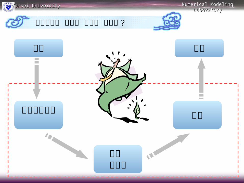
일기예보는 어떻게 만들어 지는가 ?
관측자료처리
분석
관측 예보
수치 모델링

Numerical Modeling Laboratory
Numerical Modeling Laboratory
Yonsei UniversityYonsei University
일기예보는 어떻게 만들어 지는가 ?
Step1: 관측
Step2: 자료처리
• 지상기상관측
• 고층기상관측 레이다관측
• 위성기상관측
• 해양기상관측
• 통신용 컴퓨터를 통한 전세계 기상자료의 수집 → 편집 , 가공
• 수집된 기상자료로 각종일기도와 예보자료를 작성

Numerical Modeling Laboratory
Numerical Modeling Laboratory
Yonsei UniversityYonsei University
대기현상 법칙은 ?
열역학 법칙
역학 법칙
• 열역학 제 2 법칙 → 에너지보존
열 = 에너지 + 일 p
v
H c T p
c T p
V00000000000000
( 가속도 )
힘 = 질량 × 가속도
• 질량 ≒ 1 kg/m³
• 힘 : 기압경도력 , 코리올리힘 , 마찰력 … 공기 ~
1kg/m³
rF
pF
cF

운동량 보존
질량 보존
수분 보존
이상기체 방정식
에너지 보존 ( 열역학 법칙 )
Numerical Modeling LaboratoryNumerical Modeling Laboratory
대기 현상의 법칙 ?지배 방정식
질량의 시간변화 = 0
수분의 시간변화 = 증발 - 응결
열 = 에너지 + 일
F : 기압경도력 , 중력 , 마찰력 , 원심력 , 코리올리힘 F ma
10
dM
M dt
dqE C
dt
p RT
v
dT dQ C p
dt dt

Numerical Modeling Laboratory
Numerical Modeling Laboratory
Yonsei UniversityYonsei University
V. Bjerknes (1904) pointed out for the first time that there is a complete set of
7 equations with 7 unknowns that governs the evolution of the atmosphere:
2d
pdt
v
F v- (1-3) 운동량 보존
The governing equations
.( )t
v (4)
이상기체 상태방정식 (5)
질량 보존 ( 연속방정식 )
1p
ds d QC
dt dt T
(6)
dqE C
dt 수증기 보존 (7)
열역학 제 1 법칙 ( 에너지 보존 )
p RT
7 equations, 7 unknown (u,v,w,T, p, den and q)solvable

컴퓨터 모델을 이용하여 대기의 운동을 지배하는 역학과정과 물리과정을 수식으로 풀어 미래 대기의 상태를 예측하는 것 .
Numerical Modeling LaboratoryNumerical Modeling Laboratory
수치예보란 ??
1. 관 측
2. 자료처리 3. 수치모델링 4. 분 석
5. 예 보
보다 정확한 물리과정보다 정학한 초기자료 예측성 향상 !!
Numerical Modeling Laboratory
Numerical Modeling Laboratory
Yonsei UniversityYonsei University
수치 예보의 역사
1904 : Norwegian V. Bjerknes (1862-1951) :날씨 예측 방법의 수학적 표현 기상 예보 위한 방정식 개발
1922 : British L. F. Richardson (1881-1953) :
수치 예측 모형 개념 정립 및 최초 계산 시도 ( 실패 )1. 원시방정식 사용2. 계산불안정3. 초기 조건의 문제점
1939 : Swedish C.-G. Rossby : 비발산 와도 방정식 개발 큰 규모 행성파 예측 1948, 1949, J. G. Charney (1917-1981)
Scale analysis 를 통하여 작은 규모 운동 제거 지균풍 가정 : 정역학방정식과 지균풍방정식 이용
소규모 파동 제거 , 일기의 변화에 중요한 영향 미치는 큰 규모
파동만 남김( 순압 준지균 잠재와도 방정식 )
1950 : Princeton Group (Charney, Fjortoft, von Newman)
ENIAC (Electrical Numerical Integrator and Computer) 첫 수치예보에 성공 !
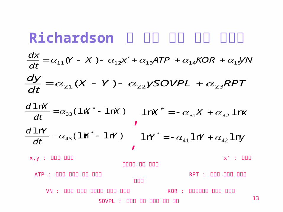
수치예보의 선구자 L.F. Richardson, 그리고 정치학
연세대학교 홍성유
13
Richardson 의 군비 예측 수치 방정식
VNKORATPxXYdt
dx1514131211 )(
RPTySOVPLYXdt
dy232221 )(
)ln(lnln *
33 XXdt
Xd xXX lnln 3231
* ,)ln(ln
ln *43 YY
dt
Yd
, yYY lnlnln 4241*
x,y : 소련의 국방비 x′ : 전쟁에 사용하지 않은 국방비
ATP : 미국이 소련에 대한 긴장감 RPT : 소련이 미국에 느끼는 긴장감
VN : 미국이 베트남 전쟁에서 지출한 국방비 KOR : 한국전쟁에서 지출한 국방비
SOVPL : 소련의 경제 제도에 대한 지수
14
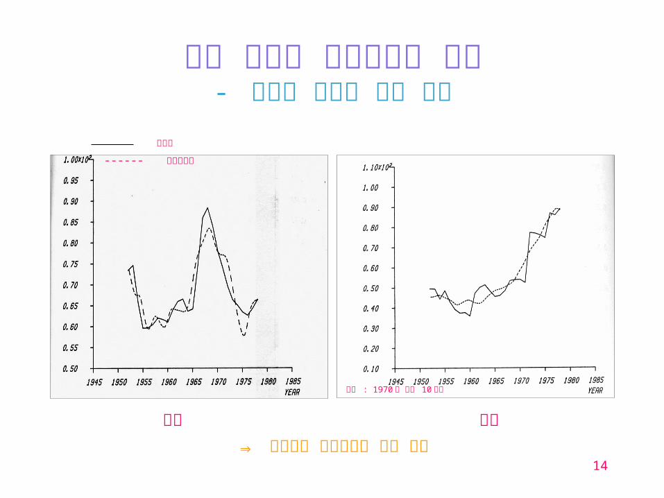
실제 자료와 시뮬레이션 결과- 국방비 예산의 연별 경향
미국 소련
실제값
------ 시뮬레이션
단위 : 1970 년 미화 10 억불
⇒ 기상학의 수치모형과 매우 유사

15
25
35
45
55
65
75
1950 1960 1970 1980 1990 2000
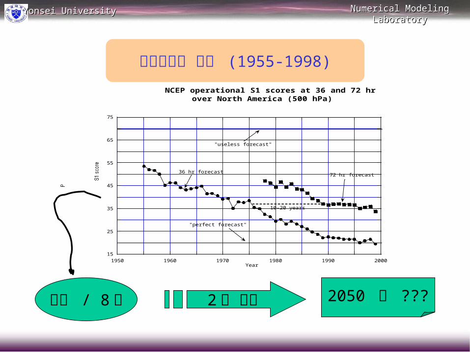
NCEP operational S1 scores at 36 and 72 hrover North America (500 hPa)
Year
"useless forecast"
"perfect forecast"
72 hr forecast36 hr forecast
10-20 years
예측오차의 경향 (1955-1998) : 미국기상청
하루 / 8 년
Numerical Modeling Laboratory
Numerical Modeling Laboratory
Yonsei UniversityYonsei University
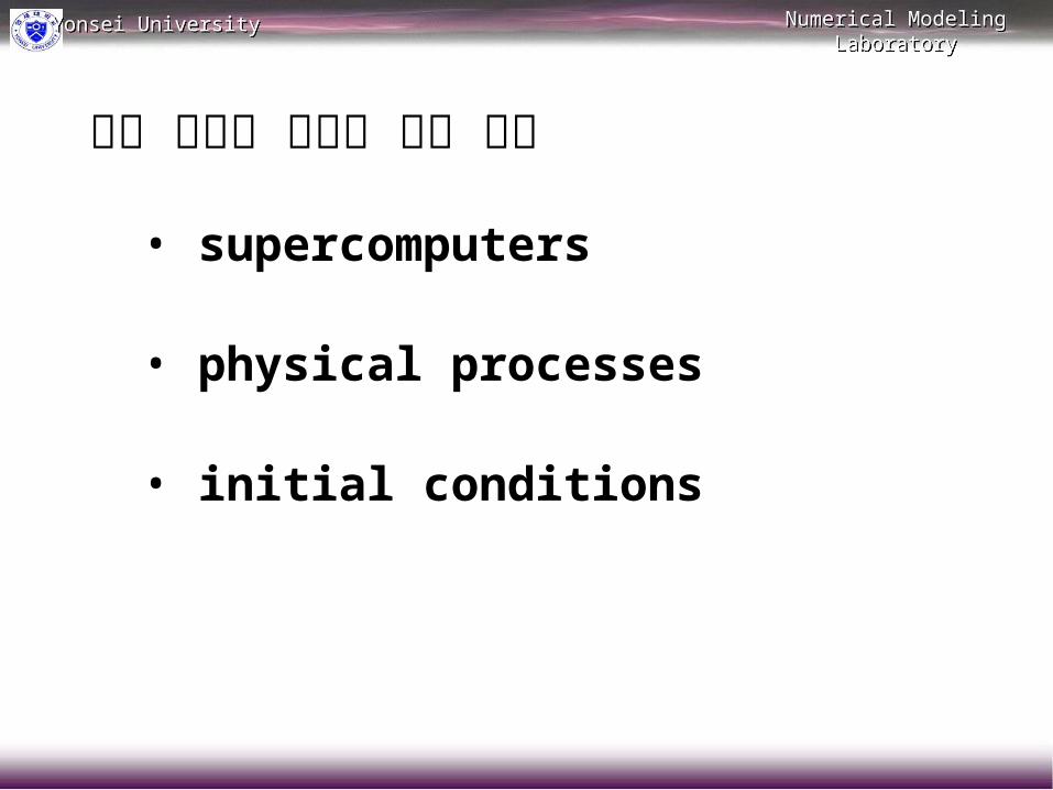
수치 예보의 예측성 향상 원인
• supercomputers
• physical processes
• initial conditions

Numerical Modeling Laboratory
Numerical Modeling Laboratory
Yonsei UniversityYonsei University
Supercomputers
18
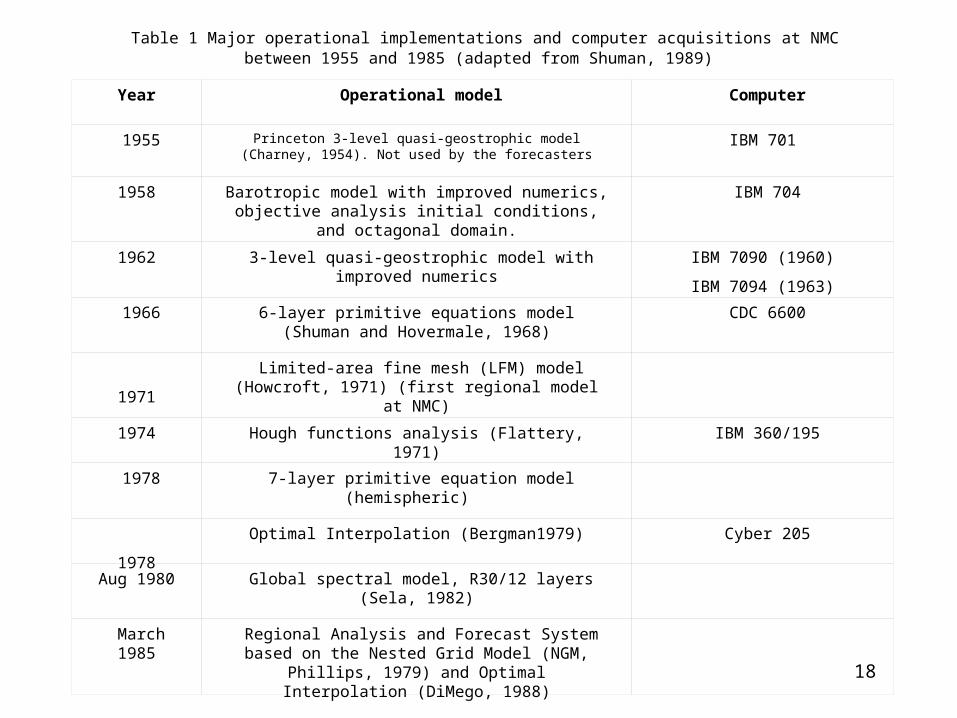
Table 1 Major operational implementations and computer acquisitions at NMC between 1955 and 1985 (adapted from Shuman, 1989)
Year Operational model Computer
1955 Princeton 3-level quasi-geostrophic model (Charney, 1954). Not used by the forecasters
IBM 701
1958 Barotropic model with improved numerics, objective analysis initial conditions, and octagonal domain.
IBM 704
1962 3-level quasi-geostrophic model with improved numerics
IBM 7090 (1960)
IBM 7094 (1963)
1966 6-layer primitive equations model (Shuman and Hovermale, 1968)
CDC 6600
1971
Limited-area fine mesh (LFM) model (Howcroft, 1971) (first regional model at NMC)
1974 Hough functions analysis (Flattery, 1971) IBM 360/195
1978 7-layer primitive equation model (hemispheric)
1978
Optimal Interpolation (Bergman1979) Cyber 205
Aug 1980 Global spectral model, R30/12 layers (Sela, 1982)
March 1985 Regional Analysis and Forecast System based on the Nested Grid Model (NGM, Phillips, 1979) and Optimal
Interpolation (DiMego, 1988)

19
Table 2: Major changes in the NMC/NCEP global model and data assimilation system since 1985 (from a compilation by P. Caplan, pers. comm., 1998)
Year Operational model Computer acquisition
April 1985
GFDL physics implemented on the global spectral model with silhouette orography, R40/ 18 layers
Dec 1986 New Optimal Interpolation code with new statistics
1987 2nd Cyber 205
Aug 1987
Increased resolution to T80/ 18 layers, Penman-Montieth evapotranspiration and other improved physics (Caplan and White, 1989, Pan, 1989)
Dec 1988 Implementation of Hydrostatic Complex Quality Control (Gandin, 1988)
1990 Cray YMP/8cpu/
32megawordsMar 1991 Increased resolution to T126 L18 and improved physics, mean
orography. (Kanamitsu et al, 1991)
June 1991 New 3D Variational Data Assimilation (Parrish and Derber, 1992, Derber et
al, 1991)
Nov 1991 Addition of increments, horizontal and vertical OI checks to the CQC (Collins and Gandin, 1990)
7 Dec 1992 First ensemble system: one pair of bred forecasts at 00Z to 10 days, extension of AVN to 10 days (Toth and Kalnay, 1993, Tracton and Kalnay, 1993)
Aug 1993 Simplified Arakawa-Schubert cumulus convection (Pan and Wu, 1995). Resolution T126/ 28 layers
Jan 1994 Cray C90/16cpu/
128megawordsMarch 1994 Second ensemble system: 5 pairs of bred forecasts at 00Z, 2
pairs at 12Z, extension of AVN, a total of 17 global forecasts every day to 16 days

20
10 Jan 1995 New soil hydrology (Pan and Mahrt, 1987), radiation, clouds, improved data assimilation. Reanalysis model
25 Oct 1995 Direct assimilation of TOVS cloud-cleared radiances (Derber and Wu, 1997). New PBL based on nonlocal diffusion (Hong and Pan,
1996). Improved CQC
Cray C90/16cpu/
256megawords
5 Nov 1997 New observational error statistics. Changes to assimilation of TOVS radiances and addition of other data sources
13 Jan 1998 Assimilation of non cloud-cleared radiances (Derber et al, pers.comm.). Improved physics.
June 1998
Resolution increased to T170/ 40 layers (to 3.5 days). Improved physics. 3D ozone data assimilation and forecast. Nonlinear increments in 3D VAR. Resolution reduced to T62/28levels on Oct. 1998 and upgraded back in
Jan.2000
IBM SV2 256 processors
June 2000
Ensemble resolution increased to T126 for the first 60hrs
May 2001 NEW cloud scheme, convection scheme, SSMI data assimilation
2002 MRF 254,L64
2005 GFS 382, L64
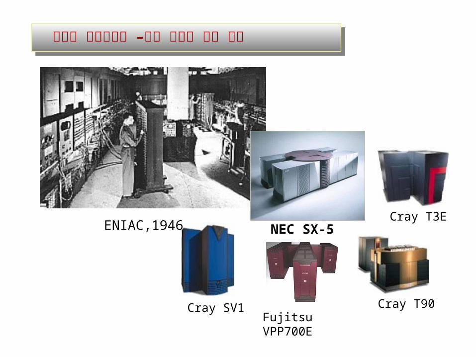
Cray T90
Cray T3E
Cray SV1Fujitsu VPP700E
NEC SX-5ENIAC,1946
고성능 수퍼컴퓨터 –수치 모델과 함께 발달
Initial condition(data assimilation : 자료동화 )
10
15
20
25
30
35
40
45
50
1975 1980 1985 1990 1995 2000
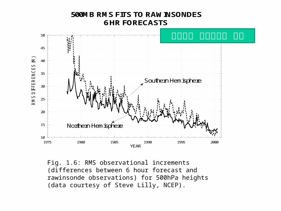
500MB RMS FITS TO RAWINSONDES6 HR FORECASTS
A
YEAR
RM
S D
IFFE
RE
NC
ES
(M
)
Southern Hemisphere
Northern Hemisphere
Fig. 1.6: RMS observational increments (differences between 6 hour forecast and rawinsonde observations) for 500hPa heights (data courtesy of Steve Lilly, NCEP).
북반구가 남반구보다 좋음
Numerical Modeling Laboratory
Numerical Modeling Laboratory
Yonsei UniversityYonsei University
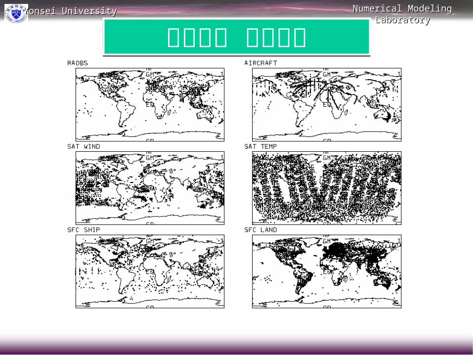
여러가지 관측자료여러가지 관측자료

Data Assimilation
• Model 1°X 1° resolution, 20 levels
u, v, T, q, Ps, Tg6 6360 180 20 1.3 10 4 var 5 10iabl
• observation : 4 510 ~ 10 non-uniform distribution
3 hour window
• Data assimilation cycle 1) data checking
2) objective analysis
3) Initialization: dynamical adjustment
4) short-range fcst for first guess
Global analysis (statistical interpolation) and balancing
Observation (+/-3hrs) Background of FG
Initial Conditions
Global forecast model
(operational forecasts)
6 hour forecast
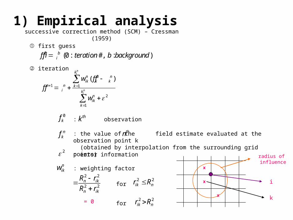
1) Empirical analysissuccessive correction method (SCM) – Cressman
(1959)① first guess
0 (0 : #, : )bi if f iteration b background
② iteration0
1 1
2
1
( )ni
ni
kn nik k k
n n ki i k
nik
k
w f ff f
w
nkf
0kf : observation
: the value of the field estimate evaluated at the observation point k (obtained by interpolation from the surrounding grid points)
2
thk
thn
: error information
nikw
2 2
2 2n ik
n ik
R r
R r
2 2ik nr R
2 2ik nr R
: weighting factor
= 0
for
for
x
x
x
i
k
radius of influence
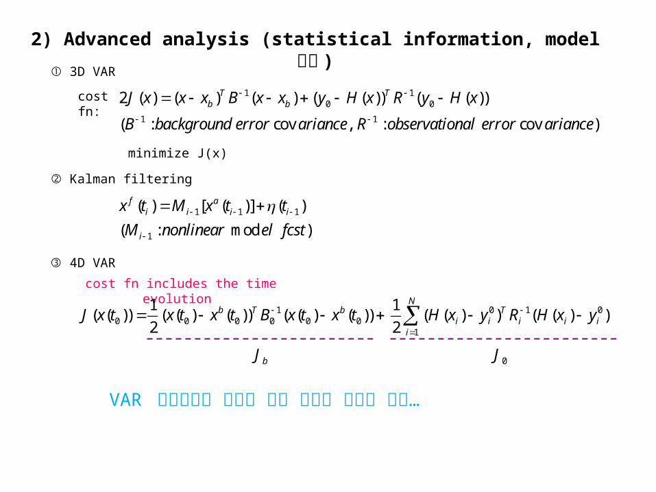
2) Advanced analysis (statistical information, model 사용 )
① 3D VAR
cost fn: 1 10 0
1 1
2 ( ) ( ) ( ) ( ( )) ( ( ))
( : cov , : cov )
T Tb bJ x x x B x x y H x R y H x
B background error ariance R observational error ariance
minimize J(x)
② Kalman filtering
1 1 1
1
( ) [ ( )] ( )
( : mod )
f ai i i i
i
x t M x t t
M nonlinear el fcst
③ 4D VAR
cost fn includes the time evolution
1 0 1 00 0 0 0 0 0
1
1 1( ( )) ( ( ) ( )) ( ( ) ( )) ( ( ) ) ( ( ) )
2 2
Nb T b T
i i i i ii
J x t x t x t B x t x t H x y R H x y
bJ 0J
VAR 초기자료는 모델의 역학 열역학 조건에 부합…

Standard 4D-Var
Initial guess
Forward Integration
NLM X, J
▽J ADJM
Backward Integration
Observations
Minimization Process
Revised Initial Conditions

Numerical Modeling Laboratory
Numerical Modeling Laboratory
Yonsei UniversityYonsei University
Model - Dynamics : Speed - Physics : Predictability
Numerical Modeling Laboratory
Numerical Modeling Laboratory
Yonsei UniversityYonsei University
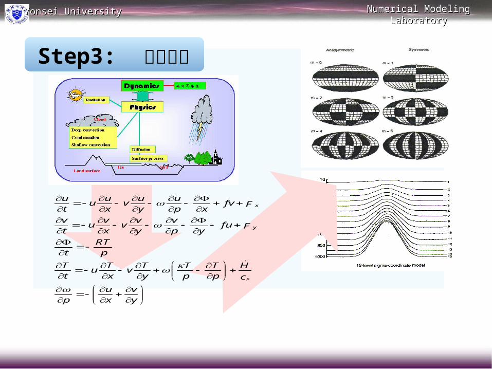
Step3: 수치적분
y
v
x
u
p
c
H
p
T
p
T
y
Tv
x
Tu
t
T
p
RT
t
Ffuyp
v
y
vv
x
vu
t
v
Ffvxp
u
y
uv
x
uu
t
u
p
y
x
31
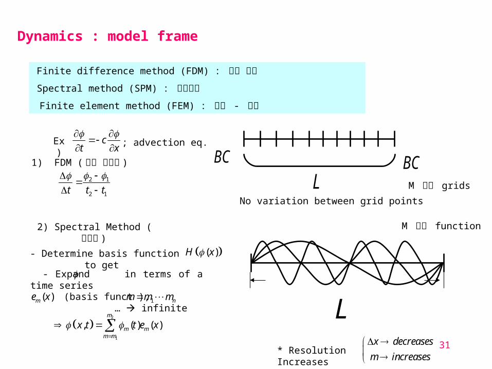
ct x
Ex)
; advection eq.
1) FDM ( 유한 차분법 )
BC BCL2 1
2 1t t t
Finite difference method (FDM) : 지역 모형
Spectral method (SPM) : 전구모형
Finite element method (FEM) : 중간 - 공학
Dynamics : model frame
No variation between grid points
M 개의 grids
2) Spectral Method ( 분광법 )
M 개의 function
- Determine basis function to get
( )H x
- Expand in terms of a time series
(basis funct ), … infinite ( )me x 1 nm m m
2
1
, ( ) ( )m
m mm m
x t t e x
* Resolution Increases
x decreases
m increases
L

Numerical Modeling LaboratoryNumerical Modeling Laboratory
수치모델링Dynamics
Physics
강수과정
단파복사
기압경도력 , 중력 , 원심력 , 코리올리힘 ..
장파복사
난류효과
현열 , 잠열
지면마찰효과
식생작용
해수면온도
적운대류
오염물질
온실기체
O3
Numerical Modeling LaboratoryNumerical Modeling Laboratory
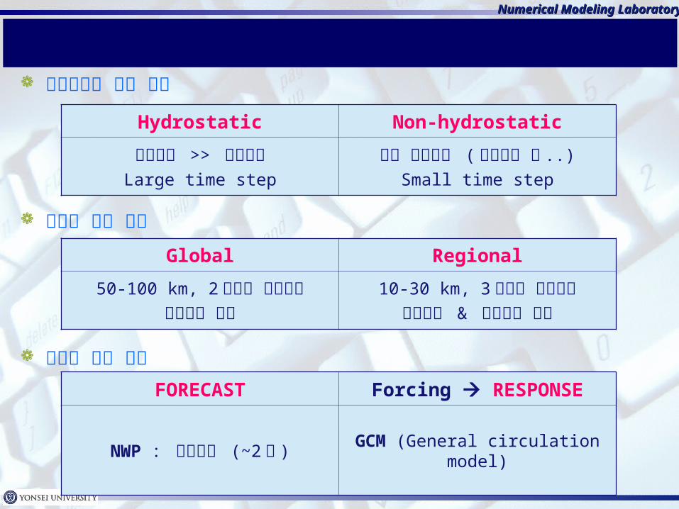
수치예보 모델의 분류
역학체계에 의한 구분
규모에 의한 구분
목적에 따른 구분
Hydrostatic Non-hydrostatic
수평규모 >> 연직규모Large time step
작은 수평규모 ( 집중호우 등 ..)Small time step
Global Regional
50-100 km, 2 주까지 예보가능초기조건 필요
10-30 km, 3 일까지 예보가능초기조건 & 경계조건 필요
FORECAST Forcing RESPONSE
NWP : 단기예보 (~2 주 )GCM (General circulation
model)

Numerical Modeling Laboratory
Numerical Modeling Laboratory
Yonsei UniversityYonsei University
수치 모델링
대기과학의 집합체
대기역학 대기물리
Numerical Modeling Laboratory
Numerical Modeling Laboratory
Yonsei UniversityYonsei University
NML

Numerical Modeling LaboratoryNumerical Modeling Laboratory
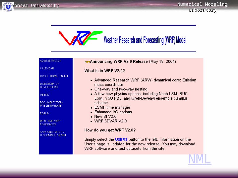
WRF Model
The Weather Research and Forecasting Model (WRF)
Mesoscale grid model
Global model
Mesoscale model
관측 및 자료처리
Numerical Modeling LaboratoryNumerical Modeling Laboratory
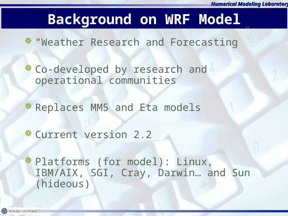
Background on WRF Model “Weather Research and Forecasting”
Co-developed by research and operational communities
Replaces MM5 and Eta models
Current version 2.2
Platforms (for model): Linux, IBM/AIX, SGI, Cray, Darwin… and Sun (hideous)
Numerical Modeling LaboratoryNumerical Modeling Laboratory
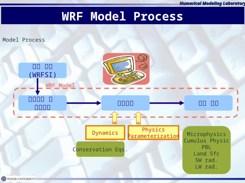
WRF Model Process
Model Process
PhysicsParameterization
초기자료 및 경계자료 수치적분 모형 결과
Dynamics
Conservation Eqs.
MicrophysicsCumulus Physic
PBLLand SfcSW rad.LW rad.
자료 생성(WRFSI)
WRF Model

Numerical Modeling LaboratoryNumerical Modeling Laboratory
WRF Model Process
Numerical Modeling LaboratoryNumerical Modeling Laboratory
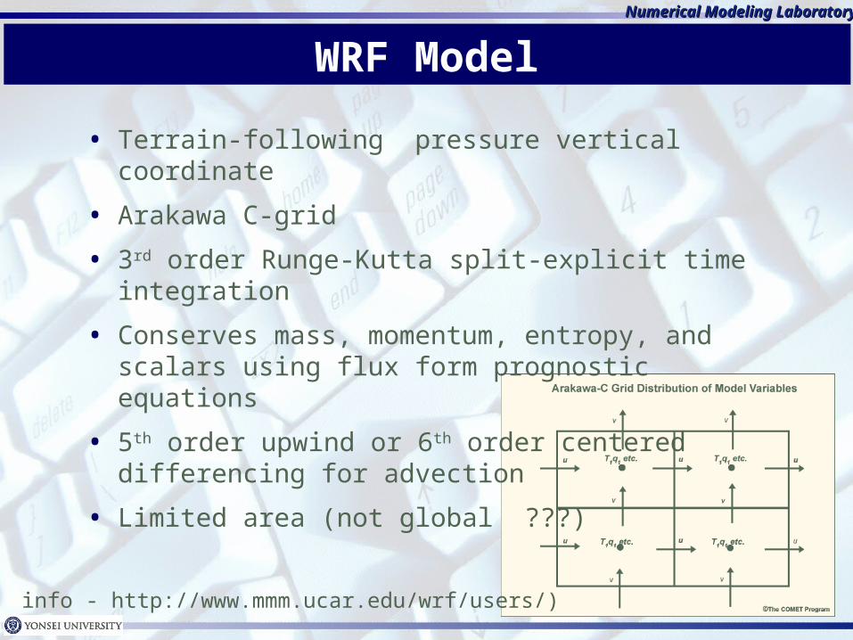
WRF Model
• Terrain-following pressure vertical coordinate
• Arakawa C-grid
• 3rd order Runge-Kutta split-explicit time integration
• Conserves mass, momentum, entropy, and scalars using flux form prognostic equations
• 5th order upwind or 6th order centered differencing for advection
• Limited area (not global ???)
(more info - http://www.mmm.ucar.edu/wrf/users/)

WRF 구름물리과정
Numerical Modeling Laboratory
Numerical Modeling Laboratory
Yonsei UniversityYonsei University
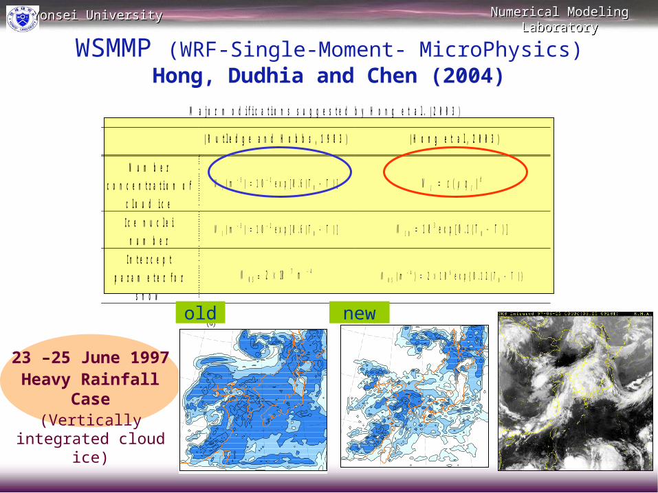
M a j o r m o d i f i c a t i o n s s u g g e s t e d b y H o n g e t a l . ( 2 0 0 3 )
( R u t l e d g e a n d H o b b s , 1 9 8 3 ) ( H o n g e t a l , 2 0 0 3 )
N u m b e r
c o n c e n t r a t i o n o f
c l o u d i c e
3 20( ) 1 0 e x p [ 0 . 6 ( ) ]IN m T T ( ) d
I IN c q
I c e n u c l e i
n u m b e r 3 2
0( ) 1 0 e x p [ 0 . 6 ( ) ]IN m T T 30 01 0 e x p [ 0 . 1 ( ) ]IN T T
I n t e r c e p t
p a r a m e t e r f o r
s n o w SN 0 = 7102 4m 4 6
0 0( ) 2 1 0 e x p { 0 . 1 2 ( ) }SN m T T
old new
WSMMP (WRF-Single-Moment- MicroPhysics)Hong, Dudhia and Chen (2004)
23 –25 June 1997Heavy Rainfall
Case(Vertically integrated
cloud ice)
Numerical Modeling Laboratory
Numerical Modeling Laboratory
Yonsei UniversityYonsei University
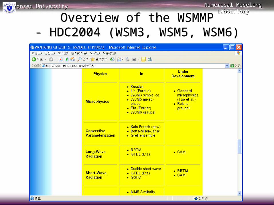
Overview of the WSMMP- HDC2004 (WSM3, WSM5, WSM6)
Overview of the WSMMP- HDC2004 (WSM3, WSM5, WSM6)

Numerical Modeling Laboratory
Numerical Modeling Laboratory
Yonsei UniversityYonsei University
Idealize 2D squall line experiment- 250 m horizontal resolution
WSM6WSM6WSM5WSM5WSM3WSM3
Precipitation
Hydrometer
WSM6 WSM5
WSM3
Numerical Modeling Laboratory
Numerical Modeling Laboratory
Yonsei UniversityYonsei University
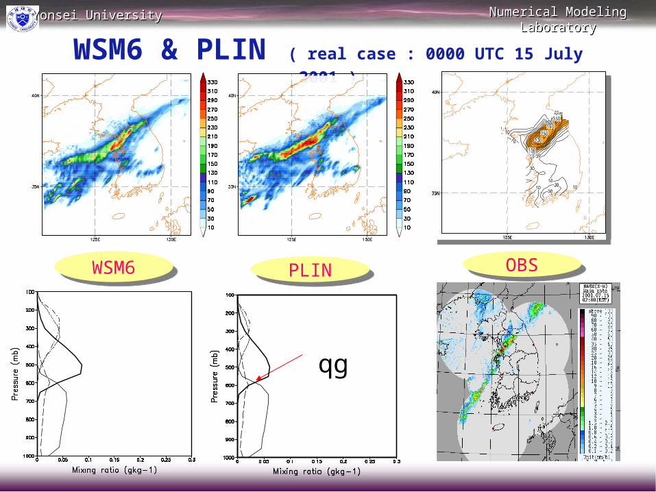
Comparison of WSM6 and PLIN - Hong et al. (2006, to be submitted to Mon.
Wea.Rev.)
Comparison of WSM6 and PLIN - Hong et al. (2006, to be submitted to Mon.
Wea.Rev.)

Numerical Modeling Laboratory
Numerical Modeling Laboratory
Yonsei UniversityYonsei University
Comparison of WSM6 and Lin
WSM6WSM6 PLINPLIN
Water vapor
Rain
Cloud ice
Snow
Cloud water
Piacr, Psacr
Pgfrz, P
iacr, Psa
cr, Pgacr
Pimlt
Pihmf, Pihtf
Pgmlt, Pgeml
Pcond
Pra
ci,
Psa
ci,
Psa
ut
Praci,
PgaciPsacw, Pgacw
Pra
ut,
Pra
cw,
Psa
cw,
Pgacw
Pracs, Pgacs, Pgaut
Psmlt, Pseml
Graupel
Pidep, Pigen
Pidep
Psdep
Psdep,Psevp
Pgdep
Pgdep
, Pgevp
Prev
p
Water vapor
Rain
Cloud ice
Snow
Cloud water
Piacr, Psacr
Pgfrz, P
iacr, Psa
cr, Pgacr
Pimlt
Pihmf
Pgmlt
Pcond
Pra
ci,
Psa
ci,
Psa
ut,
Psfi
Praci,
PgaciPsacw, Pgacw
Pra
ut,
Pra
cw,
Psa
cw,
Pgacw
Pracs, Pgacs, Pgaut
Psmlt
Graupel
Pidep
Pidep
Psdep
Psdep
Pgdep
Pgdep, P
gevp
Prev
p
Psfw
Water vapor
Rain
Cloud ice
Snow
Cloud water
Piacr, Psacr
Pgfrz, P
iacr, Psa
cr, Pgacr
Pimlt
Pihmf
Pgmlt
Pcond
Pra
ci,
Psa
ci,
Psa
ut,
Psfi
Praci,
PgaciPsacw, Pgacw
Pra
ut,
Pra
cw,
Psa
cw,
Pgacw
Pracs, Pgacs, Pgaut
Psmlt
Graupel
Pidep
Pidep
Psdep
Psdep
Pgdep
Pgdep, P
gevp
Prev
p
Psfw
Numerical Modeling Laboratory
Numerical Modeling Laboratory
Yonsei UniversityYonsei University
WSM6 & PLIN ( real case : 0000 UTC 15 July 2001 )
qg
WSM6WSM6 PLINPLIN OBSOBS

WRF-SINGLE-MOMENT-MICROPHYSICS SCHEME
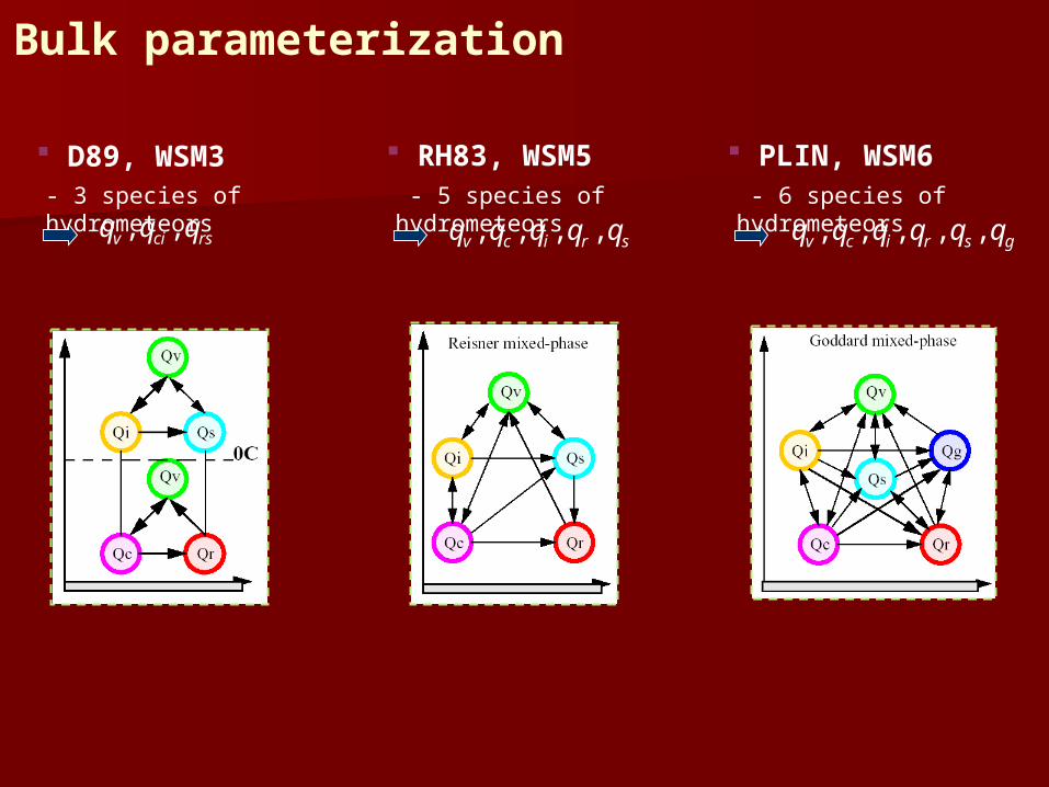
Bulk parameterization
RH83, WSM5 - 5 species of hydrometeors, , , ,v c i r sq q q q q
D89, WSM3- 3 species of hydrometeors, ,v ci rsq q q
PLIN, WSM6 - 6 species of hydrometeors, , , , ,v c i r s gq q q q q q
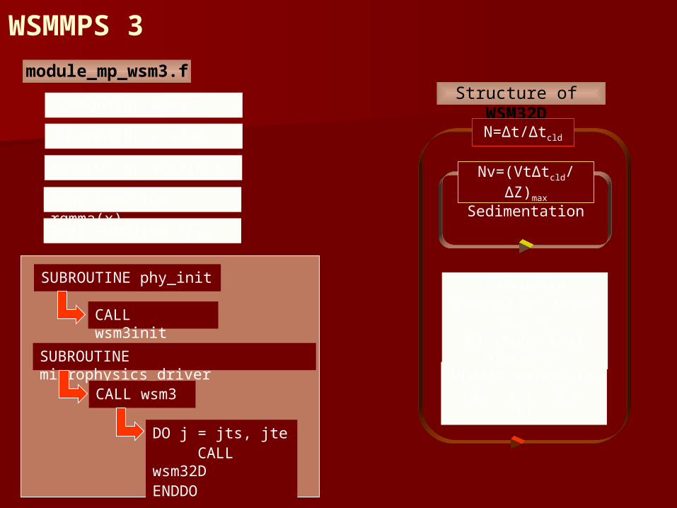
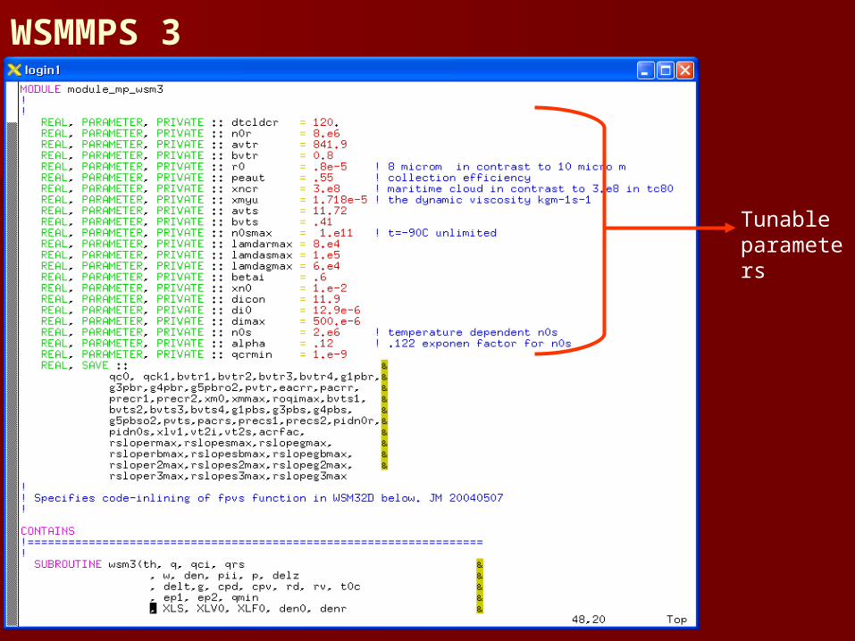
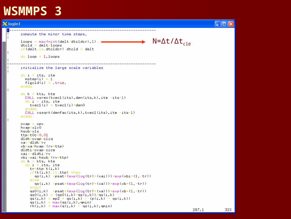
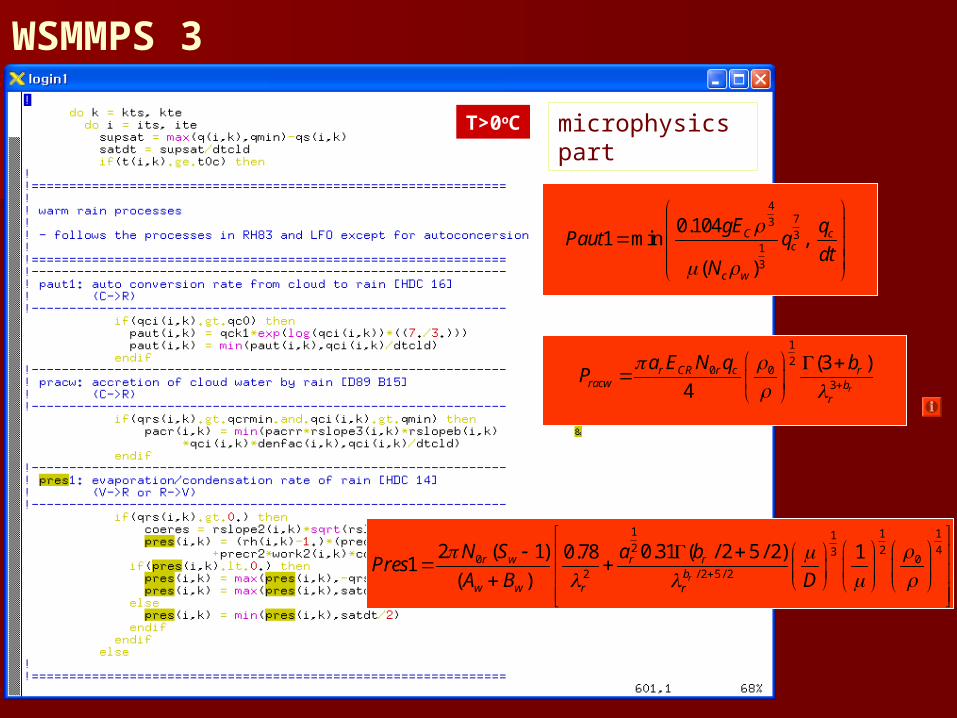
WSMMPS 3
Calculate production terms due to
Microphysical processes
Sedimentation
Structure of WSM32D
N=Δt/Δtcld
Nv=(VtΔtcld/ΔZ)max
Update variables(qv, qci, qrs, T)
module_mp_wsm3.f
SUBROUTINE wsm3
SUBROUTINE wsm32D
SUBROUTINE wsm3init
REAL FUNCTION rgmma(x)
REAL FUNCTION fpvs
SUBROUTINE microphysics_driver
CALL wsm3
SUBROUTINE phy_init
CALL wsm3init
DO j = jts, jte CALL wsm32DENDDO

WSMMPS 3T>0oC
T≤0oC
qrs (rain)
q (vapor)
qrs (snow)qci (ice)
qci (cloud)paut1pracw
paut2praci
pres1
pres2
pcon
pisdpgen
• paut1 : autoconversion of cloud water • pcon : condensation • pres1 : evaporation/condensation of rain • pracw : accretion of cloud water by rain
• pgen : generation(nucleation) of ice from vapor• pisd : Deposition/Sublimation rate of ice• pres2 : deposition/sublimation rate of snow • paut2 : conversion(aggregation) of ice to snow• praci : accretion of cloud ice by snow
T>0oC
T≤0oC
WSMMPS 3
Tunable parameters

WSMMPS 3
Define functions
WSMMPS 3
N=Δt/Δtcld

WSMMPS 3
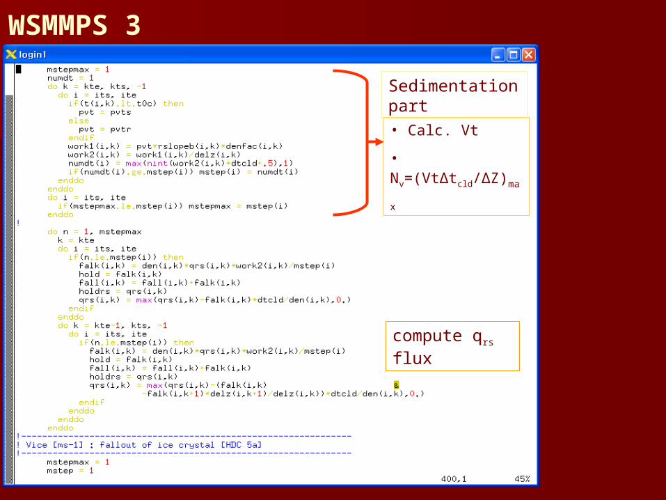
Sedimentation part
1
21 0(4 ) 1
[ ]6 r
r rr b
r
a bV ms
WSMMPS 3
• Calc. Vt
• Nv=(VtΔtcld/ΔZ)max
Sedimentation part
compute qrs flux

WSMMPS 3
Sedimentation part
WSMMPS 3
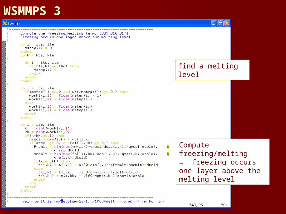
find a melting level
Compute freezing/melting→ freezing occurs one layer above the melting level
WSMMPS 3
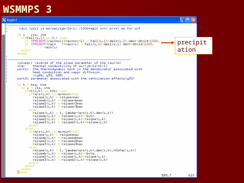
precipitation
WSMMPS 3
microphysics partT>0oC
4733
1
3
0.1041 min ,
( )
C cc
c w
gE qPaut q
dtN
1
20 0
3
(3 )
4 r
r CR r c rracw b
r
a E N q bP
1 1 112 2 43
0 02 / 2 5 / 2
2 ( 1) 0.31 ( / 2 5 / 2)0.78 11
( ) r
r w r rb
w w r r
N S a bPres
A B D

WSMMPS 3
microphysics partT≤0oC
psaci
1
20 0
03
(3 ), exp[0.05( )]
4 s
s SI s i ssaci SIb
s
a E N q bP E T T
1
2 4 ( 1)11.9 i i i
i i i
q n SPisd
n A B
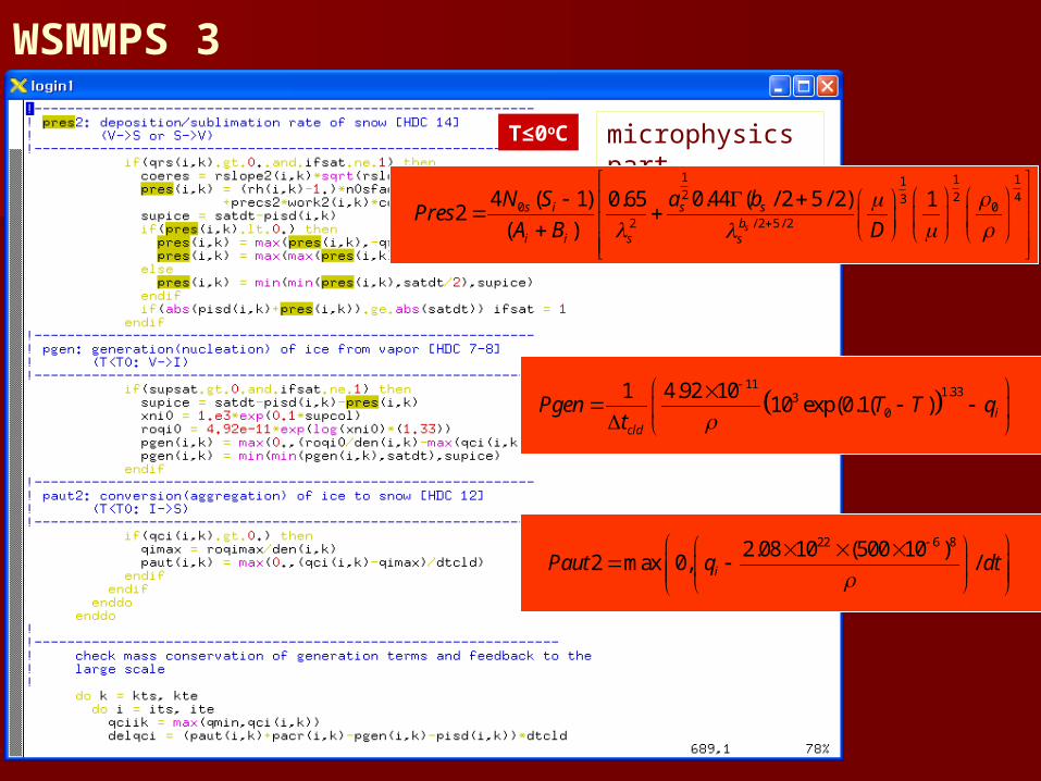
WSMMPS 3
microphysics partT≤0oC
22 6 82.08 10 (500 10 )2 max 0, /iPaut q dt
1 1 112 2 43
0 02 / 2 5 / 2
4 ( 1) 0.44 ( / 2 5 / 2)0.65 12
( ) s
s i s sb
i i s s
N S a bPres
A B D
11
1.3330
1 4.92 1010 exp(0.1( ) i
cld
Pgen T T qt

WSMMPS 3
update part
mass conservation check
update qv, qci, qrs, T

WSMMPS 3
update part
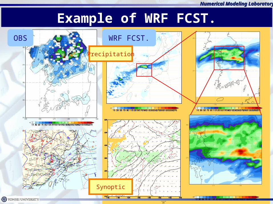
Numerical Modeling LaboratoryNumerical Modeling Laboratory
Example of WRF FCST.OBS WRF FCST.
Precipitation
Synoptic

▪ 연세대 : 1984-5 년 연구용 준지균 역학 모형 개발
차세대 수치모형 : YOURS
▪ 서울대 : 1986-1987 년 : VAX - MM4 run ( 폭설 사례 ) 1987-1989 년 : 1984 년 8.31-9.1 일 서울 호우 모의
▪ 기상청 : 1989 년 7 월 22 일 : 기상청 예비 모의 시작 1992 년 제한 지역 모형 현업 시작 (KLAPS) 1998 년 전구모형 현업 시작
한국의 수치예보

연구도구로서의 수치모델연구도구로서의 수치모델
역학적 , 열역학적 특성 연구
민감도 실험 (physics, external forcing)
Mechanism 규명
중요 forcing 규명
New theory 개발
시간 공간적 고해상도의 자료
Numerical Modeling Laboratory
Numerical Modeling Laboratory
Yonsei UniversityYonsei University
화남지방에 상륙한 태풍과 한반도 집중호우와의 관련성
김 계 환 ( 공군 ), 홍 성 유연세대 대기과학과
Numerical Modeling Laboratory
Numerical Modeling Laboratory
Yonsei UniversityYonsei University
0%
10%
20%
30%
40%
50%
60%
70%
80%
90%
100%
150 250 350
Precipitation (mm)
Ratio(%
)
0
5
10
15
20
25
30
35
150 250 350 850
Precipitation(mm)
Fre
quency
(num
ber)
0%
10%
20%
30%
40%
50%
60%
70%
80%
90%
100%
N TC R TC P TC + R TC
Ratio (
%)
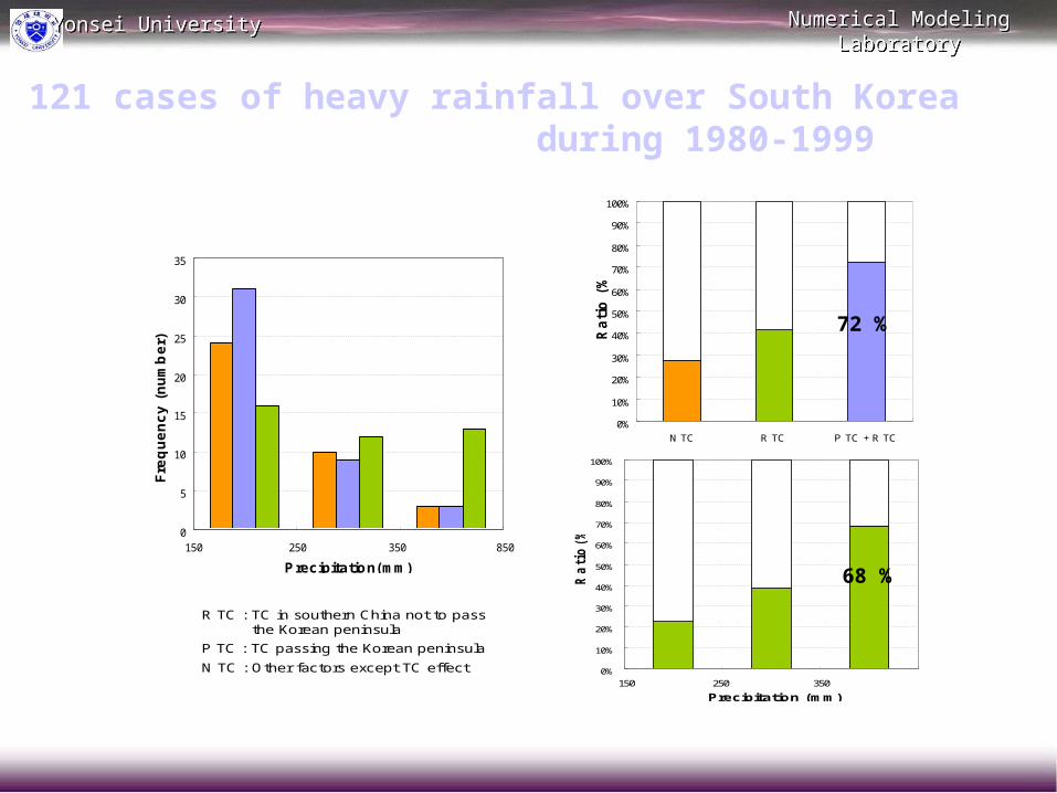
R TC : TC in southern China not to passthe Korean peninsula
P TC : TC passing the Korean peninsula
N TC : Other factors except TC effect
72 %
68 %
121 cases of heavy rainfall over South Korea during 1980-1999

Numerical Modeling Laboratory
Numerical Modeling Laboratory
Yonsei UniversityYonsei University
Heavy rainfall at Kanghwa during 1200 UTC 4-1200 UTC 6 August, 1998
00 03 06 09 12 15 18 21 00 (UTC)05AUG 06AUG
(mm)
120
90
60
30
0
00 03 06 09 12 15 18 21 00 (UTC)05AUG 06AUG
(mm)
120
90
60
30
0
Numerical Modeling Laboratory
Numerical Modeling Laboratory
Yonsei UniversityYonsei University
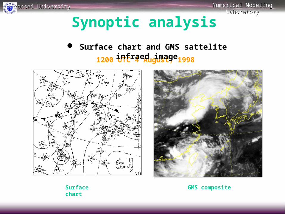
Synoptic analysis
1200 UTC 4 August, 1998
Surface chart GMS composite
Surface chart and GMS sattelite infraed image
Numerical Modeling Laboratory
Numerical Modeling Laboratory
Yonsei UniversityYonsei University
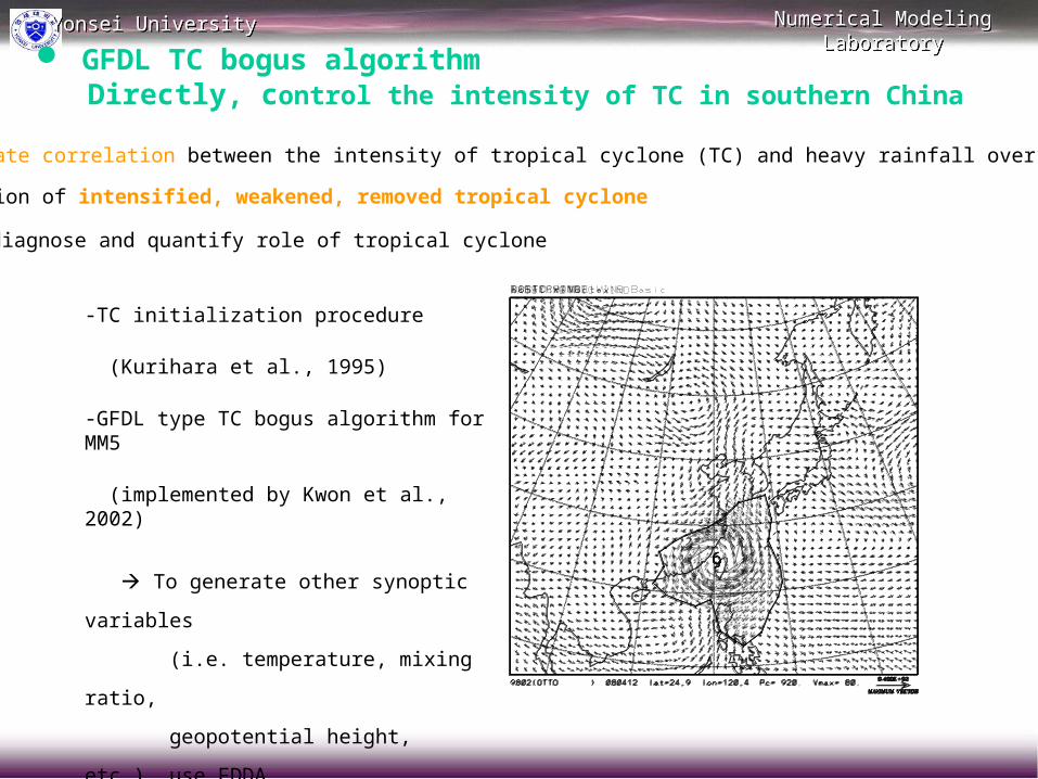
GFDL TC bogus algorithm Directly, control the intensity of TC in southern China
Intimate correlation between the intensity of tropical cyclone (TC) and heavy rainfall over Korea
Adoption of intensified, weakened, removed tropical cyclone
diagnose and quantify role of tropical cyclone
-TC initialization procedure
(Kurihara et al., 1995)
-GFDL type TC bogus algorithm for MM5
(implemented by Kwon et al., 2002)
To generate other synoptic
variables
(i.e. temperature, mixing ratio,
geopotential height, etc.), use
FDDA
(Four Dimensional Data
Assimilation)
in MM5 option.

Numerical Modeling Laboratory
Numerical Modeling Laboratory
Yonsei UniversityYonsei University
Model & experiments
Model MM5 version 3
Phsical option
Micro phsics Mixed phase
Cumulus Kain-Fritsch
PBL Blackadar
Radiation RRTM
Map projection
Lambert conformal
Domain Domain 1 Domain 2
Resolution 45km 15km
Grid size 141*141 121*121
Integration time
60 s 20 s
Vertical size 23 sigma layer (model top : 100 hPa)
Iintial data& Lateralboundary
Data
NCEP reanalysis data&
GTS
Model set-up
Numerical Modeling Laboratory
Numerical Modeling Laboratory
Yonsei UniversityYonsei University
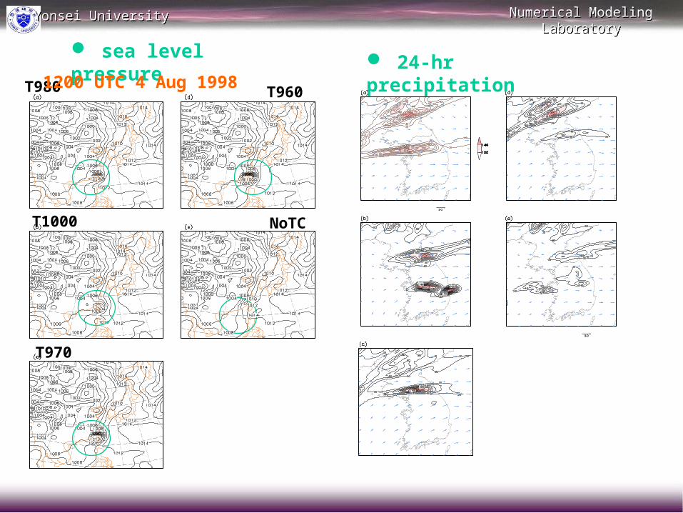
sea level pressure
T970
T980
T1000
T960
NoTC
1200 UTC 4 Aug 1998 24-hr precipitation

Numerical Modeling Laboratory
Numerical Modeling Laboratory
Yonsei UniversityYonsei University
불확실성
Numerical Modeling Laboratory
Numerical Modeling Laboratory
Yonsei UniversityYonsei University
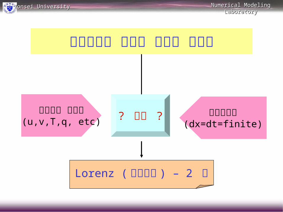
수치모형을 이용한 대기의 예측성
? 한계 ?대기현상 복잡성(u,v,T,q, etc)
계산상오차(dx=dt=finite)
Lorenz ( 혼돈역학 ) – 2 주
Numerical Modeling Laboratory
Numerical Modeling Laboratory
Yonsei UniversityYonsei University
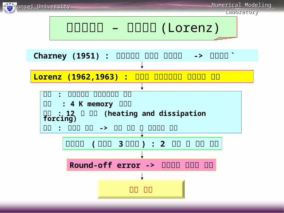
예측성이론 – 혼돈역학 (Lorenz)
Charney (1951) : 초기자료와 모델의 불확실성 -> 예측한계 `
Lorenz (1962,1963) : 불안정 역학시스템의 주기성의 한계
목적 : 수치모형이 통계모형보다 좋음도구 : 4 K memory 컴퓨터모델 : 12 개 변수 (heating and dissipation forcing)결과 : 변수의 변화 -> 수년 적분 후 비주기성 확인
초기조건 ( 소수점 3 째자리 ) : 2 개월 후 다른 결과
Round-off error -> 비주기성 결과의 원인
혼돈 역학
Numerical Modeling Laboratory
Numerical Modeling Laboratory
Yonsei UniversityYonsei University
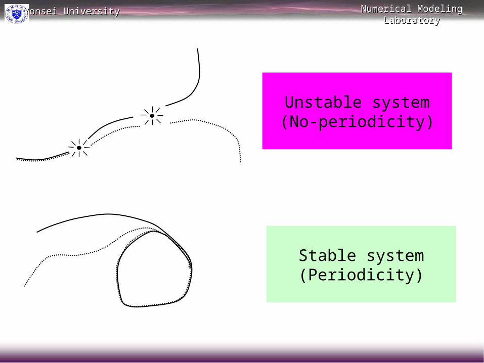
Unstable system(No-periodicity)
Stable system(Periodicity)

Numerical Modeling Laboratory
Numerical Modeling Laboratory
Yonsei UniversityYonsei University
앙상불 예보

Numerical Modeling Laboratory
Numerical Modeling Laboratory
Yonsei UniversityYonsei University
time
stochastic
deterministic
Transition : 2-3 days for largesccaleflows
2-3 hours for individual thunderstorm
Shorter for sharply nonlinear parameters
(precip. Diverges faster than 500 mb Z

Numerical Modeling Laboratory
Numerical Modeling Laboratory
Yonsei UniversityYonsei University
0
0.2
0.4
0.6
0.8
1
0 5 10 15
Anomaly Correlation for the winter of 1997/98 (from 00Z)Controls (T126 and T62) and 10 perturbed ensemble forecasts
mrf126
forecast day
Average of 10 perturbed forecasts
Individualperturbed forecasts
Control (deterministic)forecasts, T126 and T62
anom
aly
corr
ela
tion
Ensemble ( 앙상블 예보 )
Numerical Modeling Laboratory
Numerical Modeling Laboratory
Yonsei UniversityYonsei University
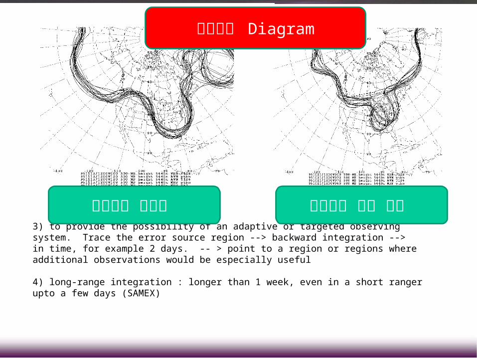
3) to provide the possibility of an adaptive or targeted observing system. Trace the error source region --> backward integration --> in time, for example 2 days. -- > point to a region or regions where additional observations would be especially useful
4) long-range integration : longer than 1 week, even in a short ranger upto a few days (SAMEX)
예보관이 신뢰함 예보관이 신뢰 못함
스파게티 Diagram
Numerical Modeling Laboratory
Numerical Modeling Laboratory
Yonsei UniversityYonsei University
예측성 한계

Numerical Modeling Laboratory
Numerical Modeling Laboratory
Yonsei UniversityYonsei University
수치모형을 이용한 대기의 예측성
? 한계 ?대기현상 복잡성(u,v,T,q, etc)
계산상오차(dx=dt=finite)
Lorenz ( 혼돈역학 ) – 2 주
Numerical Modeling Laboratory
Numerical Modeling Laboratory
Yonsei UniversityYonsei University
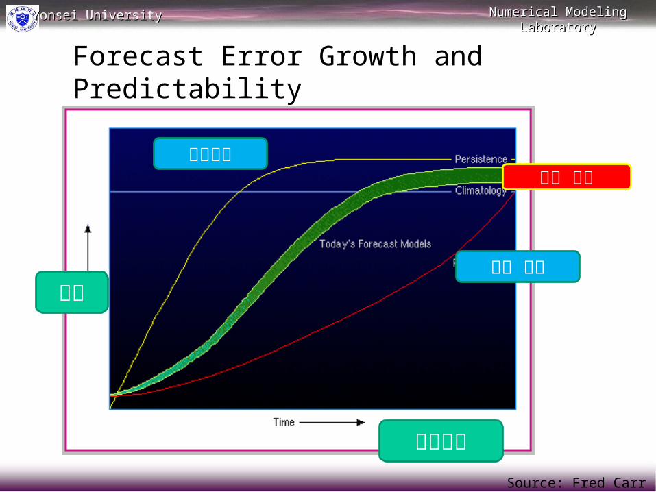
Forecast Error Growth and Predictability
Source: Fred Carr
예측시간
오차완전 모델
종관예보현재 수준
Numerical Modeling Laboratory
Numerical Modeling Laboratory
Yonsei UniversityYonsei University
15
25
35
45
55
65
75
1950 1960 1970 1980 1990 2000
NCEP operational S1 scores at 36 and 72 hrover North America (500 hPa)
Year
"useless forecast"
"perfect forecast"
72 hr forecast36 hr forecast
10-20 years
예측오차의 경향 (1955-1998)
2 주 까지 하루 / 8 년 2050 년 ???


![Data Assimilation for Numerical Weather Prediction - [NWP ......Data Assimilation for Numerical Weather Prediction [NWP] Project Ahmed Attia Statistical and Applied Mathematical Science](https://img.dokumen.tips/doc/110x75/6039cba9995b992a170c4a78/data-assimilation-for-numerical-weather-prediction-nwp-data-assimilation.jpg)


