On the Empirical Distribution of the Balassa Index files/ballassa wwa.pdf · 1 I. INTRODUCTION The concept of “revealed comparative advantage” as defined by Bela Balassa is widely

0

On the Empirical Distribution of the Balassa Index

Jeroen HINLOOPEN

University of Amsterdam and Delft University of Technology

Charles van MARREWIJK

Erasmus University Rotterdam

Published as: Hinloopen, J., and C. van Marrewijk (2001), “On the empirical distribution of the

Balassa index,” Review of World Economics / Weltwirtschaftliches Archiv 137: 1-35.

February, 2000; Revised August, 2000

CONTENTS:

I Introduction

II The Balassa Index

III Shape, stability and aggregation over time

IV Persistence

V Regional differences

VI Conclusions

REMARK: We would like to thank, without implicating, Leendert Punt for excellent assistance.

An earlier version of this paper was presented at CEPR’s 1998 European Research Workshop on

International Trade. We are grateful to an anonymous referee for detailed and constructive

comments, and to Harry Bowen, Stephen Martin, Stephen Redding, Teun Schmidt and workshop

participants at the University of Copenhagen and the CPB (Netherlands Bureau for Economic

Policy Analysis) for useful comments. Thanks are also due to the Dutch Japanese Trade

Association (Dujat) for making available the data. Any errors are, of course, our responsibility.

1

I. INTRODUCTION

The concept of “revealed comparative advantage” as defined by Bela Balassa is widely used in

practice to determine a country’s weak and strong sectors. Michael Porter, for example, uses a

Balassa Index exceeding 1, in some cases strengthened to a Balassa Index exceeding 2, to identify

a country’s strong sectors in his influential book The Competitive Advantage of Nations.1 Other

empirical examples are Ariovich (1979), Reza (1983), Yeats (1985), Peterson (1988), Crafts

(1989), and Amiti (1999). Despite detailed discussions on the Balassa Index - see Kunimoto

(1977), Hillman (1980), Bowen (1983, 1985, 1986), Balance et al. (1985, 1986, 1987), Vollrath

(1991), and Bowen et al. (1998) - the distribution of the Balassa Index cannot be derived

theoretically. In addition, the distribution has not been systematically analyzed empirically (see

also Yeats; 1985, p. 61).2 Specific values of the Balassa Index are therefore difficult to interpret.

Moreover, it is a priori not clear that a particular value for the Balassa Index implies the same

extent of comparative advantage for different countries.

We provide a systematic analysis of the empirical distribution of the Balassa Index. To

determine this distribution we could, in principle, proceed in two alternative directions. First, we

could take the world as a whole as the group of reference countries and consider all exports of all

countries. Second, we could select a group of similar countries for reference purposes and

investigate export flows for these countries only. There are several disadvantages to the first

approach. Not only could it be that countries at very different levels of (economic) development

are being compared, disturbing influences in the export flows are also not being controlled for.

Consider, for example, the export of flowers to Germany, either from The Netherlands or from

1 Additional selection criteria were also used by Porter, see Porter (1990, pp. 739-740) for details. 2 Hillman (1980), for example, develops a necessary and sufficient monotonicity condition under identical homothetic preferences for the correspondence between the Balassa Index and pre-trade relative prices for a particular industry in two different countries. In our data set the Hillman condition was violated for 7.0 percent of the export value (somewhat smaller than the 9.5 percent found by Marchese and Nadal de Simone; 1989), and for less than 0.5 percent of the number of observations. Since the distributions of the Balassa Index reported below are based on the number of observations we conjecture that our findings are not affected by the Hillman critique.

2

Kenya. Since, like Germany, The Netherlands are a member of the European Union, access to the

German market is easier for the Dutch than for the Kenyans.3 Moreover, as a neighbour the Dutch

incur much lower transport costs to reach the German market than do the Kenyans.

To circumvent these difficulties we take the second approach mentioned above. That is, we

analyse the export performance of similar countries to a third market. For that we have selected

the Member States of the European Union as the reference countries and consider export flows to

Japan. Apart from concentrating on countries with a comparable level of economic development

which all incur similar transport cost, there are two additional reasons for this selection; access to

the relatively homogenous Japanese market is, in principle, the same for all Member States of the

European Union, and the Japanese market is large enough to generate substantial export flows for

a representative array of products. Accordingly, the results presented in this paper provide

“clean” insights as to the statistical properties of the Balassa Index.4

To analyze in detail the empirical distribution of the Balassa Index we proceed as follows. In

section II we briefly discuss the Balassa Index and describe the data. In section III, we consider

the Balassa Index for the EU-12 as a whole, that is, we group all observations for the different

countries together. Both the effect of aggregation of export flows over time on the EU-wide

distribution of the Balassa Index is considered, as well as its stability over time. Observe that

there are (at least) two types of stability: (i) stability of the distribution of the Balassa Index from

one period to the next, and (ii) stability of the value of the Balassa Index for a particular industry

and country from one period to the next. The first type of stability is analyzed in section III. The

second type of stability is analyzed in section IV. The persistence issues addressed in section IV,

for which we analyze Markovian transition probability matrices, give insights into the behaviour

of a particular industry’s comparative advantage over time. Section V investigates the empirical

3 On the restrictions imposed on the import of flowers into the European Union see European Commission (1995, chapter 6).

3

distribution of the Balassa Index for the Member States separately. Although these distributions

also appear to be stable over time (type i stability), they differ markedly between nations. This

indicates that a particular value of the Balassa Index has a different meaning for different

countries.

Our main conclusions, see also section VI, can be summarized as follows. In all cases the

distribution of the Balassa Index is very skewed with a median well below one, a mean well

above one, and a monotonically declining density function. The process is apparently well

defined in the sense that the distribution changes very little from one period to the next.

Moreover, aggregation over time of export flows, that is analyzing annual rather than monthly

trade flows, or pooling values of the Balassa Index, either based on montly or annual flows, has

only a mild influence on the distribution. The observations for individual industries are, however,

more persistent over time for annual than for monthly trade flows. The widely used criterium

"Balassa Index > 1" to identify sectors with a comparative advantage selects about one third of

the exporting industries. Finally, we note that the distribution of the Balassa Index differs

considerably across countries, making comparisons of the index between countries problematic.

This certainly holds for the dynamic properties of the process. Although different mobility

indices based on our estimated transition probability matrices do not always lead to the same

ranking, within our sample of countries Germany appears to have the most persistent and Greece

the most mobile pattern of comparative advantage over time.

II. THE BALASSA INDEX

Although Liesner (1958) was the first to utilize an index of revealed comparative advantage, the

most frequently used measure in this respect is called the “Balassa Index”, after the refinement

and popularization by Balassa (1965, 1989). Given a group of reference countries the Balassa

4 Ignoring exports to other countries outside the European Union could yield biased results. However, since the export flows to Japan are the second-largest of total extra-EU exports (the flow to the U.S. is the

4

Index basically measures normalized export shares, where the normalization is with respect to the

exports of the same industry in the group of reference countries. In particular, if XjA is country A’s

export value of industry j, Xjref is industry j’s export value for the group of reference countries,

and we define Xi = ∑j Xji for i = A,ref, then country A’s Balassa Index of revealed comparative

advantage for industry j, BIjA, equals:

(1) .//

refrefj

AAjA

j XXXX

BI =

If BIjA exceeds 1 country A is said to have a comparative advantage in industry j, since this

industry is more important for country A’s exports than for the exports of the reference countries.

For our empirical investigation we use a comprehensive data set provided by Eurostat. The

data used concern export flows (in value) from 12 Member States of the European Union

(Germany, France, The Netherlands, Belgium, Luxembourg, The United Kingdom, Denmark,

Ireland, Spain, Portugal, Italy and Greece; henceforth referred to as “EU-12”) to Japan from 1992

through 1996. The export figures are monthly data and cover all 2-digit Combined Nomenclature

industries as distinguished by Eurostat. This includes the “secret uses” category “00” (weapons,

coming from the United Kingdom, Germany and The Netherlands) and the “special uses”

category “99” (with only a few observations), but it excludes category “77” (“reserved for future

use,” with no observations). The total number of different industries therefore equals 99 (Table

A1 in the Appendix provides a brief description of all the industries). Since Luxembourg is

combined with Belgium in the observations we have 5 (years) × 12 (months) × 11 (countries) ×

99 (industries) = 65,340 non-negative observations. The actual number of positive observations

equals 47,339 (which is 72.5% of all possible observations).

The exports from the EU-12 countries to Japan (Euro 20,566 million in 1992, rising to Euro

31,957 million in 1996) are much lower than the exports from Japan to the EU-12 countries (Euro

largest) we conjecture that this possible bias is modest if at all present.

5

51,530 million in 1992, falling to Euro 49,136 million in 1996), although the gap is narrowing

slowly. To illustrate the use of the Balassa Index to identify sectors with a comparative

advantage, and to characterize the data set we performed some calculations presented in Table 1

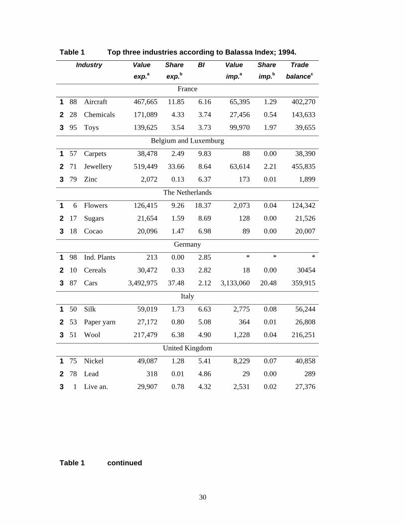
and Figure 1. First, Table 1 shows the three sectors for each country with the highest Balassa

Index in 1994, the year in the middle of our sample period, as well as the export value for these

sectors, and the share of the sector in the total exports of the country.

INSERT TABLE 1 ABOUT HERE

The sector with the highest comparative advantage in France, for example, is the aircraft

industry (BI = 6.16). With almost 500 million Euro in export value it represents a sizable share of

French exports (almost 12%). Clearly, this sector benefits from intermediate deliveries, mainly

from Spain, Germany and the United Kingdom, to the Airbus industry in Toulouse. A quick look

at the top three industries in Table 1 shows that many sectors are fairly traditional, for example

carpets and jewellery (diamants) in Belgium, flowers in Holland, cars in Germany, silk and wool

in Italy, (pork-) meat in Denmark, and cork in Portugal. In many cases the top ranking industries

represent a substantial share of a country's exports; from high to low: Danish meat (46.78%),

German cars (37.48%), Belgian jewelry (33.66%), Greek tobacco (31.18%), Irish chemicals

(28.69%), and Portuguese cork (15.53%). To illustrate that a top ranking industry in terms of the

Balassa Index, which after all is a relative measure, does not have to be an important sector for a

nation, we can look at the exports of German complete industrial plants (0.00%), English lead

(0.01%), or Belgian zinc (0.13%).

INSERT FIGURE 1 ABOUT HERE

When the Balassa Index exceeds one, the sector is identified as a sector with comparative

advantage and one would generally expect net exports to be positive. In this respect, however, we

have to be cautious since the comparative advantage is calculated with respect to a set of

reference countries which excludes Japan and, as mentioned above, the EU-12 countries have a

6

substantial trade deficit with Japan. Thus, to verify if net exports are indeed positive Table 1 also

gives the value of the imports from Japan, the share in total imports, and the trade balance for

each of the top three ranking industries. In all cases in Table 1 net trade is indeed positive.5 This

topic is analyzed further in Figure 1. First, panel a illustrates the evolution over time of the share

of industries with a Balassa Index higher than 1 and higher than 2 for the EU-12 countries

grouped together (monthly moving annual observations, see section III). As panel a shows, the

share of industries with a Balassa Index higher than 1, which are thus identified as industries with

a comparative advantage, is stable at 33% (+1%). Similarly, the share of industries with a Balassa

Index higher than 2, which could be characterized as industries with medium and strong

comparative advantage (see section IV), is stable at 17% (+1%). Second, panel b of Figure 1

shows for the industries with a Balassa Index exceeding 1 and exceeding 2, the share of those

industries with positive net exports. The share of industries with a Balassa Index higher than 1

with positive net exports is slowly rising from 72% to 83%. Similarly, the share of industries with

a Balassa Index higher than 2 with positive net exports is slowly rising from 86% to 94%. This

largely reflects the declining trade deficit of the EU-12 vis a vis Japan.

III. SHAPE, STABILITY AND AGGREGATION OVER TIME

This section analyzes three issues. First, we investigate the shape of the distribution of the

Balassa Index, focusing on the cumulative distribution, some summary statistics, and the

probability density function. Second, we investigate the stability of the distribution of the Balassa

Index over time, that is whether this distribution is the same, for example, in 1992 and in 1994 or

drastically different. Recall that in this section we will identify the second type of stability

mentioned in the introduction, tracking the evolution of individual sectors over time in section IV

below. Third, we analyze the impact of aggregation of export flows over time, that is grouping 12

5 Table 1 shows a fair number of *'s, indicating that import data are not available. Since this almost always implies that those flows are effectively zero, we put them equal to zero in Figure 1.

7

observations on monthly export flows together in one observation for an annual export flow, both

for the shape and the stability of the distribution of the Balassa Index. Subsection III.1 below

considers monthly export flows, while subsection III.2 considers annual export flows.

III.1 MONTHLY OBSERVATIONS

Panel a of Table 2 gives information on the distribution of the Balassa Index for the months of

1996. See Hinloopen and Van Marrewijk (2000)6 for the years 1992 through 1995. The results in

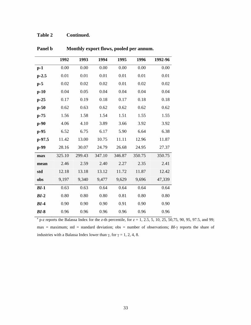
this table are pooled per annum as well as for the whole period in panel b of Table 2. In both

panels of Table 2 three types of information are listed.

First, the percentile points "p-z" are listed, where z varies from 1 to 99. This gives detailed

information on the cumulative distribution of the Balassa Index. For example, in January 1996

the p-25 point is at 0.20 (panel a), which indicates that 25% of the observations in January 1996

had a Balassa Index below 0.20 and 75% of the observations in January 1996 had a Balassa Index

above 0.20. Similarly, the p-90 point in that month was 4.24, indicating that 90% of the

observations had a Balassa Index below 4.24, and 10% above 4.24.

Second, some summary statistics on the distribution are given, in particular the maximum, the

mean, the standard deviation, and the number of observations. In January 1996 these were,

respectively, 303, 2.83, 16.4, and 762 (see panel a).

Third, the Balassa Index points "BI-z" are given, where z ranges from 1 to 8. This readily

identifies the share of industries below certain Balassa Index cut-off points. For example, in

January 1996 the BI-1 point was 0.61 (panel a), indicating that 61% of the observations in

January 1996 had a Balassa Index below 1, and thus 39% had a Balassa Index above 1. Similarly,

the BI-4 point in January 1996 is 0.89, indicating that 89% of the observations had a Balassa

Index below 4, and 11% of the observations had a Balassa Index above 4.

6 This refers to a companion paper for our analysis, which contains more details and is downloadable as pdf file and word 97 file from our personal web pages, see references.

8


The last column of panel b shows that the mean Balassa Index for the period as a whole for

monthly observations equals 2.41, almost 4 times the median Balassa Index of 0.62. This

indicates that the distribution is skewed to the right. Indeed, skewness for all observations for the

period as a whole equals 15.30, while the kurtosis is 282.81 (these values are not listed in Table

2).7 The distribution is therefore not only skewed, but also “fat tailed” (a relatively large share of

the observations is in the tails of the distribution). The median Balassa Index of 0.62 also

indicates that the “Balassa Index > 1” criterion used to identify industries with a comparative

advantage selects less than half of the industries when applied to monthly observations. More

precisely, 64% of the observations have a Balassa Index below 1, 80% have an index value below

2, 90% have an index value below 4, and 96% have an index value below 8. Put differently, the

“Balassa Index > 1” criterion applies to about 36% of the industries with positive (monthly)

exports.

Panel b of Table 2 shows also that the distribution of the Balassa Index is remarkably stable

over time if the values of the Balassa Index based on monthly export flows are pooled per annum:

the maximum (rounded) percentage point deviation of the cumulative distribution for any single

year from the (pooled total of the) period as a whole is 1%, 1%, 1% and 0% for “Balassa Index =

1, 2, 4, 8”, respectively. Panel a of Table 2 shows that this even holds for each individual month:

the maximum (rounded) percentage point deviation of the cumulative distribution for any single

month in 1996 from (the pooled total of) the period as a whole is 3%, 1%, 1% and 1% for

“Balassa Index = 1, 2, 4, 8” respectively. Also note that in all cases, that is, whether a particular

7 If μz is the z-th moment of a distribution, for z = 1,2,3,.. and σ is the standard deviation, then skewness is defined as μ3/σ3 and kurtosis as μ4/σ4. Note that these measures are dimensionless. For all symmetric distributions skewness equals 0, while skewness is positive (negative) for long tails to the right (left). Kurtosis is always positive, so that this measure is usually interpreted relative to the normal distribution which has a kurtosis of 3. Kurtosis values larger than 3 indicate fat tails (with respect to the normal distribution), while values smaller than 3 are indicative for relatively thin tails.

9

month or a particular (pooled) year is considered, at most 5% of the industries have a Balassa

Index exceeding 8.

The mean Balassa Index fluctuates more substantially over time. This comes as no surprise in

view of the very high skewness and kurtosis, which suggests the presence of outlying

observations. This also implies that the mean is a poor indicator. Consider for example the export

flows in February 1996 with 814 observations and a mean Balassa Index of 2.53, which

accommodates the maximum value of 351 for that month. Without that single maximum

observation there would be 813 observations with a mean Balassa Index of 2.10. Indeed, due to

one observation the mean increases from 2.10 to 2.53, or by more than 20%.


The findings of this subsection as summarized in Table 2 are illustrated in Figure 2. Panel 2a

shows the cumulative distribution per year (monthly observations, pooled per annum), while

panel 2b shows the cumulative distribution for the months of 1996. The distribution looks very

similar from month to month and from year to year, both in Table 2 and Figure 2. In fact, the

distribution is so stable over time that it is almost impossible to distinguish between the different

years (Figure 2, panel a), or between the different months (Figure 2, panel b).

III.2 ANUAL OBSERVATIONS

In this subsection we consider annual export flows. Observe that due to aggregation of the

monthly export flows the number of observations diminishes dramatically. However, since we

have data available on a monthly basis we would not make complete use of the information in our

dataset if we considered annual observations only from January to December. Indeed, we also

have observations for years starting in, say, April and ending in March. Combining then the best

of both worlds leads us to consider monthly moving annual observations, which gives us 46,280

observations.

10

Hinloopen and Van Marrewijk (2000) give the distribution of the Balassa Index for monthly

moving annual observations for each period for which data are available. In Table 3 this

information on annual observations is summarized and compared with monthly observations (see

also the last column of Table 2, panel b). As is to be expected, the distribution of the Balassa

Index based on annual rather than monthly observations has less extreme outliers, causing the

distribution to be more compact. The maximum falls by 29% from 351 to 250, the mean falls by

14% from 2.41 to 2.08, the standard deviation falls by 10% from 12.42 to 11.17, and the kurtosis

drops by 7% from 282.81 to 262.05. These measures are, however, dominated by relatively few

observations: as is evident from Table 3 less than 20% of the monthly observations and less than

17% of the annual observations of the Balassa Index is above the mean.


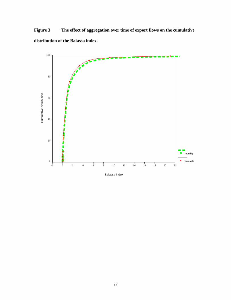
On the other hand, the shape of the cumulative distribution, which depends on the majority of

the observations, is much less affected by aggregation of export flows over time. Indeed, when

compared to Balassa indices based on monthly export flows, the share of industries with a

Balassa Index below 1, 2, 4 or 8 rises by only 3, 3, 2 and 1 percentage point(s), respectively. Also

the kurtosis changes little, from 15.30 to 15.14. This relatively mild influence of aggregation over

time on the shape of the cumulative distribution of the Balassa Index is illustrated in Figure 3.


Note that the distribution itself, based on monthly moving annual export flows, is also stable

over time (see also section III.1). This is perhaps most clearly illustrated by a comparison of the

results per annum for the period as a whole (see Table 3) with any distribution based on monthly

moving annual export flows (see Hinloopen and Van Marrewijk; 2000). This shows that the

maximum deviation for the Balassa Index at 1, 2, 4, or 8 is only 1 percentage point for all but one

"moving" year.

11

The final issue addressed in this subsection is the shape of the density function, rather than the

cumulative distribution. At various universities and seminars we asked our colleagues to sketch

their expected shape of this density function (before showing the cumulative distribution!).

Sometimes we gave them additional information, like the median and the mean. Invariably, they

sketched a bell-shaped function with a fat right tail, where the top could be either above or below

“Balassa Index = 1” (usually depending on whether or not we informed them that the median was

below 1). This, admittedly, unscientific method indicates that many economists have a poor

intuitive grasp of the shape of the density function of the Balassa Index. Our empirical results

show that the density function of the Balassa Index is not bell-shaped at all, but monotonically

declining, as shown in Figure 4.


IV. PERSISTENCE

Section III investigates the shape of the cumulative distribution of the Balassa Index and the

stability of this distribution over time, both for monthly and for annual observations. Since we

found this distribution to be rather stable over time, we can formulate statements such as “the

probability that the Balassa Index exceeds 2 in the period April 1994 - March 1995 is about

17%”. However, this type of stability does not imply that the observations for the Balassa Index

for a particular industry and country are persistent over time.

As an illustration of this point consider Figure 5. It depicts the value of the Balassa Index for

industry 6 (Live trees and other plants; bulbs, roots and the like; cut flowers and ornamental

foliage) for The Netherlands, both based on monthly observations and on monthly moving annual

observations. Clearly the value of the Balassa Index fluctuates over time, be it much less if it is

based on monthly moving annual export flows than on monthly export flows. Indeed, there may

be seasonal fluctuations in the exports of a particular industry. To the extent that these

fluctuations do not occur simultaneously in the country under investigation and the group of

12

reference countries these seasonal fluctuations lead to fluctuations in the Balassa Index which are

hard to interpret. Annual observations eliminate such difficulties of interpretation.


On the other hand, although the values of the Balassa Index in Figure 5 vary considerably,

they are always above one, both for monthly and annual data (in fact, CN-category 6 has the

highest Balassa Index for The Netherlands throughout the sample period). This suggests that

information on the value of the Balassa Index for a particular industry in a particular period is

also indicative for the value of the Balassa Index in the next period for that same industry. This

section investigates such persistence over time using transition probability matrices based on

monthly moving annual export flows.

Empirical research into the persistence and mobility of revealed comparative advantage over

time using transition probability matrices is pioneered by Proudman and Redding (1998a,b).

Although we use a similar procedure, there are also several differences. First, Proudman and

Redding (1998a) investigate 2 countries (the U.K. and Germany), extended to 5 countries (adding

France, Japan and the U.S.A.) in Proudman and Redding (1998b), whereas we investigate 12

Member States of the European Union. Second, they analyze 22 manufacturing industries,

whereas we analyze all (that is, 99) 2-digit CN industries. Third, they analyze annual OECD data

for 1970-1993, whereas we analyze monthly Eurostat data for 1992-1996. Fourth, for their

selected group of 5 countries they consider the world as a whole (approximated by the OECD

data) as a reference, without corrections in the trade data. As explained in the introduction, we

take the EU-12 countries as a reference and analyze exports to a third market (Japan) to correct

for trade biases (market access, distance, heterogeneous tastes) to get a clean measure of

comparative advantage. Fifth, they normalize the Balassa Index such that the mean is equal to one

for all countries. Since this normalization is not standard practice in applied research we did not

follow that procedure. Sixth, and finally, they endogenously divide the Balassa Index into four

13

classes to ensure that the number of observations is roughly equal for each class. Although

attractive for estimation purposes there are two main disadvantages to that approach. Not only are

the boundaries between the classes hard to interpret (what does it mean in Proudman and Redding

(1998a, p. 22) for the U.K. to have a normalized Balassa Index in the third class between 0.941

and 1.165?), but they also differ from one country to another (the third class for Germany in

Proudman and Redding (1998a, p. 22) ranges from 1.006 to 1.258). The latter makes comparisons

between countries, particularly of differences in persistence, difficult. For these reasons we divide

the Balassa Index into 4 classes which can be readily interpreted:

Class a: 0 < Balassa Index ≤ 1;

Class b: 1 < Balassa Index ≤ 2;

Class c: 2 < Balassa Index ≤ 4; and

Class d: 4 < Balassa Index.

Class a captures all those industries without a comparative advantage. The other three classes, b,

c, and d, relate to sectors with a comparative advantage, roughly divided into "weak comparative

advantage" (class b), "medium comparative advantage" (class c), and "strong comparative

advantage" (class d). The characteristics of these classes, and their differences across countries,

will become clear as we progress.

IV.1 TRANSITION PROBABILITY MATRICES

Let mabp denote a one-step transition probability, that is the probability that for monthly

observations next period’s Balassa Index of a particular sector and country fall in class b, given

that this period’s Balassa Index for that same sector and country falls in class a. Similarly, ydap

denotes the probability that for yearly observations next period’s Balassa Index of a particular

sector and country fall in class a, given that this period’s Balassa Index for that same sector and

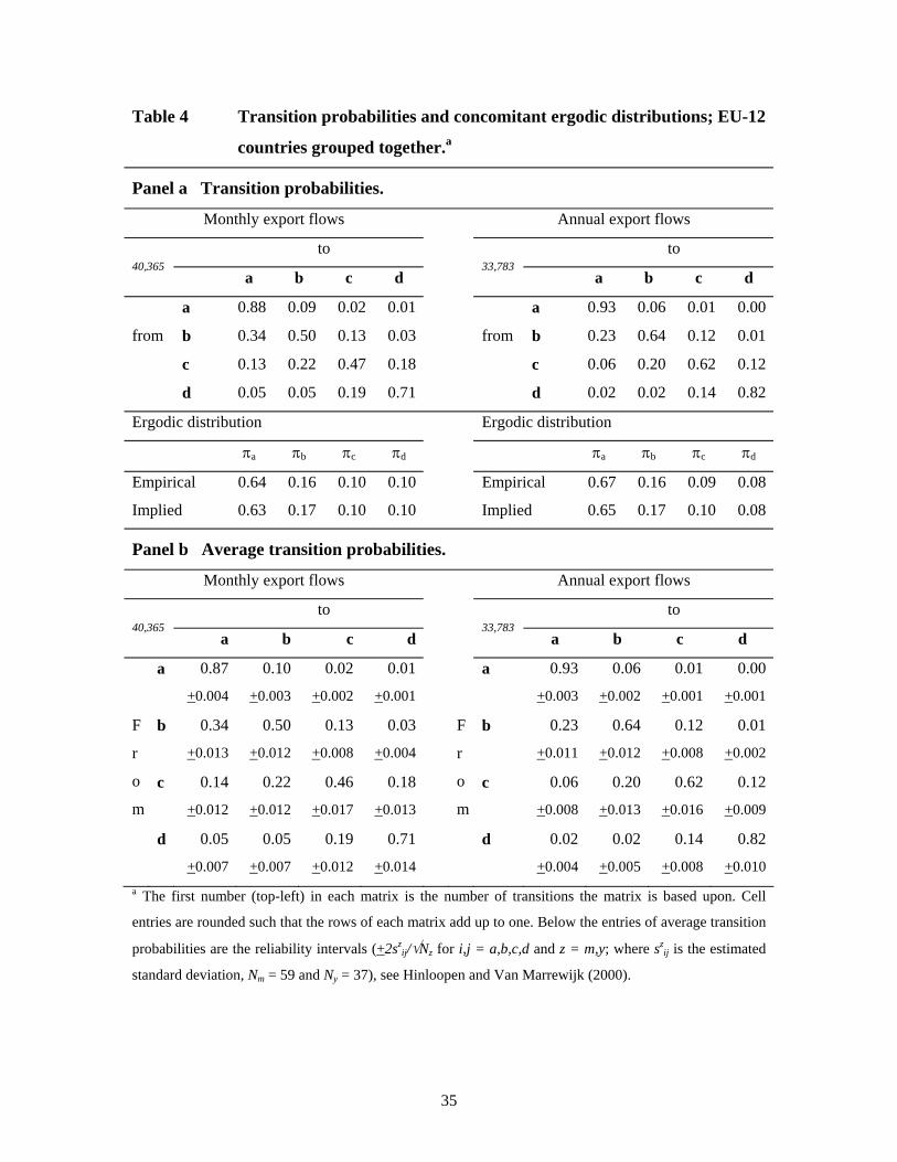
country falls in class d, etcetera. Panel a of Table 4 gives the pooled results of the one-step

14

empirical transition probabilities for all Member States considered for the period as a whole, both

monthly and annually, on the assumption that this probability is the same for all sectors and

countries. For example, panel a indicates that, given that an industry has a weak comparative

advantage in 1994 (is in class b for annual observations), the probability that it also has a weak

comparative advantage in 1995 is 64%, while the probability that it shows no comparative

advantage in 1995 is 23%, etc. Hinloopen and Van Marrewijk (2000) give all empirical, one-step,

4×4 transition probability matrices for all classes and all months, both for monthly observations

and for monthly-moving annual observations. These 59 monthly and 37 annual transition

probability matrices were used to calculate the average transition probabilities with a concomitant

95% reliability interval in Panel b of Table 4.


There is a close correspondence between the pooled and average transition probabilities: there is a

1% deviation for only 4 estimated transition probabilities for monthly flows, while there is a 0%

deviation for the other 12 monthly observations and for all annual observations. The estimated

reliability intervals are small and, with one exception, smaller for annual than for monthly flows.

The diagonal elements of the matrices in Table 4 suggest that the observations on the Balassa

Index are more persistent from period to period for both low (class a) and high (class d)

observations than for the apparently more transient intermediate classes (b and c). Moreover, as

argued above and illustrated in Figure 3, the classes appear to be more persistent for annual than

for monthly observations; all the diagonal entries, for example, are higher for annual than for

monthly observations, indicating that it is more likely to stay in the same class. Alternatively,

there is a 1% chance of moving from class a to class d for monthly observations, compared to a

0% probability for annual observation. The estimates on the reverse movements are 5% en 2%,

respectively.

15

IV.2 ERGODIC DISTRIBUTIONS

To assess whether or not the Markov transition matrices capture the underlying data-generating

process, we compute the implied limiting distribution and compare these with their empirical

counterpart. As we will see, the fit is quite good.

Assume that the transition probabilities in Table 4 are time stationary, and let Pz, for z = m,a,

be the Markov transition matrix, with pzij the probability of moving from class i to class j for z

type observations, i,j = a,b,c,d. In the terminology of Markov chains these are irreducible,

aperiodic, recurrent Markov chains with partially reflecting barriers. Further, let pijz (n) be the n-

step transition probability, i.e. the probability of going from class i to class j in n steps. If the

transition probability is stationary the matrix Pz(n), the n-step probability matrix, is simply given

by matrix multiplication: Pz(n)=Pz

n. Under these conditions (see Theorems 1.2 and 1.3, Karlin and

Taylor; 1975, pp. 83-85) the share of Balassa indices in each class a,b,c,d evolves to a stationary

probability distribution πaz, πb

z, πcz, and πd

z, the "ergodic" distribution, characterized by:

(2) ∑∑ ==≥

====∞→∞→

izij

zi

zji

zi

zi

zi

nziin

nzjin

pand

ymzanddcbajiforpp

ππππ

π

,1,0

,,,,,,limlim )()(

The top line of (2) indicates that the probability of evolving over time to any particular class is

independent of the initial class and equal to the stationary probability distribution. The bottom

line of (2) uniquely determines the πiz. It can be used to determine the stationary probability

distribution. Alternatively, one can simply calculate Pzn for large n, which is the procedure we

used, to obtain the implied stationary probability distribution (see Table 4). This result is then

compared with the empirical distribution in Table 4. These appear to be very similar, specifically

for monthly observations, suggesting that the transition probability matrices accurately

characterize the data generating process underlying the distributions of the Balassa Index.

IV.3 SECTORAL MOBILITY

16

The literature has developed a number of "mobility indices", which collapse into one number the

mobility information of a transition probability matrix, see Proudman and Redding (1998b, p.

24). Let P be the transition probability matrix, let n be the number of classes, let πi be its ergodic

distribution, where i indicates the class, and let mλ be the eigenvalues of P for m = 1,..,n.

Number the eigenvalues in declining modulus. We consider the following mobility indices,

labeled M1 - M4:8

Shorrocks (1978) )1())((1 −−= nPtrnM

Bartholomew (1973) ∑ ∑ −=k l klk lkpM π2

Shorrocks (1978) )det(13 PM −=

Sommers and Conlisk (1979) 24 1 λ−=M

Since the diagonal elements of P give the probability of staying in the same class, 1 minus these

elements give an indication of mobility, which explains M1. Since P is a transition probability

matrix there is always one eigenvalue equal to 1 and the modulus of the other eigenvalues is

bounded from above by 1. Convergence to the ergodic distribution occurs at a geometric rate

given by powers of the eigenvalues. The smaller the modulus of an eigenvalue, the faster its

corresponding component converges. Moreover, the dominant, that is the slowest, convergence

term is given by the second largest eigenvalue. Emphasizing that aspect explains M4.

Alternatively, the product of the eigenvalues is equal to the determinant of the matrix. This gives

a rationale for M3. As explained above, the size of each class evolves to the ergodic distribution.

Mobility index M2, finally, uses these as weights to calculate an extended version of M1 while

simultaneously ‘penalizing’ large movements.

Table 5 reports the mobility indices for both monthly and annual observations. All indices

indicate lower annual mobility than monthly mobility. On the face of it this seems to violate

8 Proudman and Redding (1998b) also consider ∑ −−= m m nnM ).1/()(5 λ Since all eigenvalues are real

17

Shorrocks’s (1978) period consistency criterion, as also discussed in Geweke et al. (1986),

arguing that over a longer period of observation for the same process mobility should increase.

Observe however that the process leading to the distribution of the Balassa Index based on annual

observations is not the same as the monthly process iterated 12 times. In the latter case the index

is based on a flow of exports over a one-month period and transitions are based on comparing

changes from one month to the next. For annual observations the index is based on a flow of

exports over a twelve month period and transitions are based on comparing changes from one

year to the next. Apparently, Shorrock's notion does not apply when different types of export

flows are considered.

As indicated, the Balassa indices based on annual export flows are more persistent (in the

sense of lower mobility) than those based on monthly export flows. A particular value of the

Balassa Index based on annual export flows is therefore more likely to reflect the ‘true’

comparative advantage. Accordingly, for the remainder of the analysis, which is concerned with

regional differences, we use (monthly moving) annual export flows.

V. REGIONAL DIFFERENCES

Sections III and IV focus on the shape of the distribution of the Balassa Index and its stability

over time. To that end the individual observations of different EU-12 member states are grouped

together. That, however, bypasses a range of interesting questions to be addressed on differences

in degree of specialization and mobility between countries (see also Proudman and Redding;

1998a, 1998b). Indeed, in most cases practitioners calculating Balassa indices are interested in

comparing the outcome for different countries. This section investigates these spatial differences

and finds them to be quite large. At this point we stress, however, that although the distribution

and the transition probabilities may vary from one country to another, the stability of the

for our matrices M5 equals M1.

18

distribution itself and of the transition matrices is comparable to the results found and discussed

for the EU-12 as a whole in sections III and IV.

V.1 DIFFERENT DISTRIBUTIONS

Table 6 summarizes the results on the distribution of the Balassa Index for individual countries

based on monthly moving annual export flows. There appears to be considerable country to

country variation. For example, on average 33% of the EU-12 industries has a Balassa Index

above 1 (see Table 3), but this ranges from a low of 18% for Ireland to a high of 42% for France.

Similarly, on average 8% of the EU-12 industries has a Balassa Index above 4, where the country

observations vary from 21% for Greece to 0% for Germany.


If anything, the results presented in Table 6 show that the same value for the Balassa Index

has a different meaning for different countries. Accordingly, using the Balassa Index to identify a

country’s weak and strong sectors in comparison to other countries should be done with care. On

the other hand, using the Balassa Index to rank a country’s exporting industries is not disputed by

the results presented in Table 6.

V.2 DIFFERENT TRANSITION PROBABILITIES

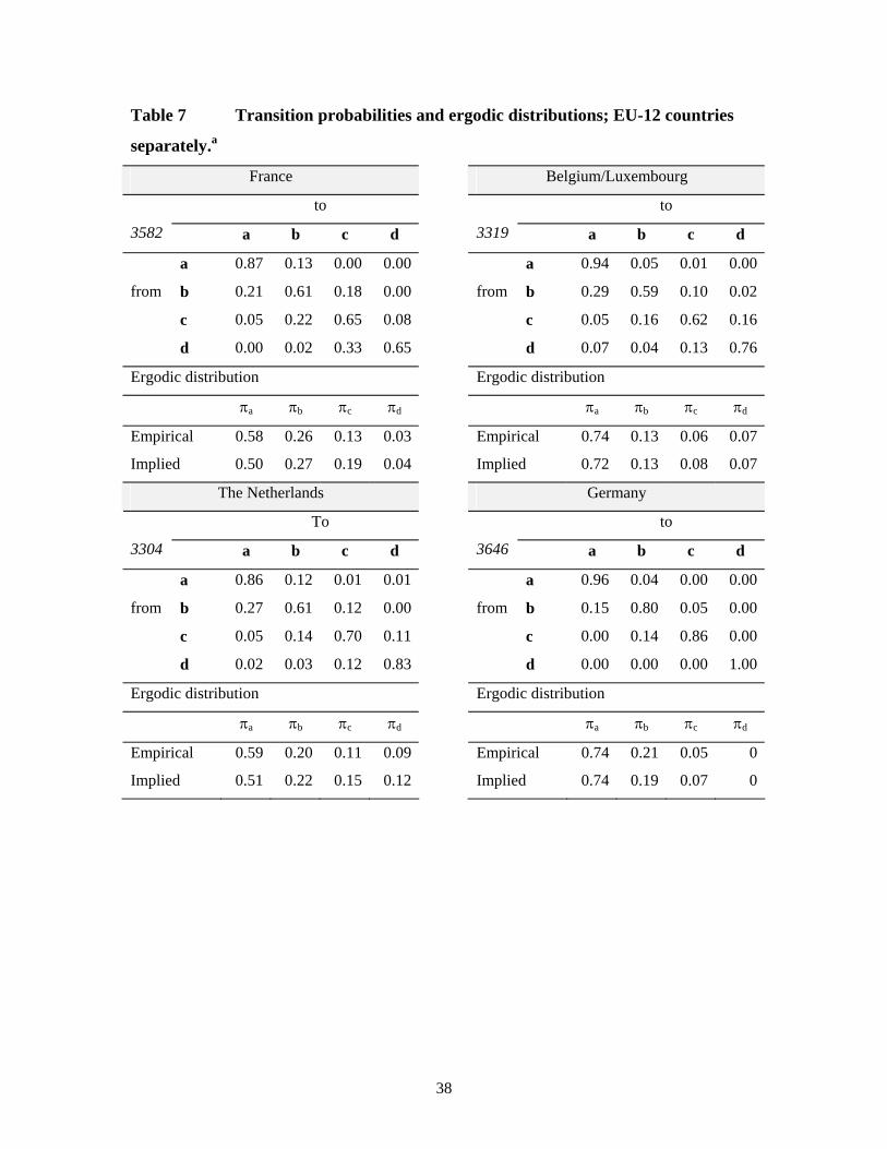
Table 7 reports the estimated pooled transition probability matrices for each EU-12 country for

the classes a-d as defined in section IV (see our webite for the estimated average transition

probability matrices).9 Again, there appears to be considerable variation, this time in transition

probabilities between the EU-12 countries. For example, the probability that an industry which

portrays no comparative advantage in a particular year remains in the same class (that is, does not

9 Since Germany has no industries with a Balassa Index exceeding 8 its estimated transition probability matrix is confined to the classes a-c only.

19

portray a comparative advantage the next year either) varies from 86% for The Netherlands to

97% for Denmark. Similar variation can be identified for the other three classes.

Below each estimated transition matrix the implied ergodic distribution is reported as well as

the empirical counterpart. In most cases the implied and empirical distribution are similar,

indicating that the transition probability matrices adequately capture the underlying distribution.

Accordingly, the transition probability matrices can be used to investigate differences in mobility

between the EU-12 Member States. Table 8 reports the four mobility indices defined in section

IV for each country, where the ordering of countries is roughly from persistent to mobile.

Proudman and Redding (1998b) estimate similar mobility indices for France, the UK and

Germany. For these countries they find a consistent ranking, being that France has the most

mobile trade specialization pattern while that of Germany is the most persistent. We find the same

ranking for each mobility index for these three countries. It is unclear at this point whether a high

or low mobility index is beneficial for the macro-economic development of a nation. As the

European soccer player of the last century10 has taught us: every disadvantage has its advantage.

In fact, this point is part of our ongoing research program.

INSERT TABLES 7 AND 8 ABOUT HERE

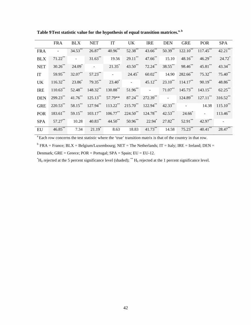
A formal confirmation that the dynamics of the Balassa Index is different for each

country is given in Table 9, which summarizes the findings on country-by-country testing for

equal transition probability matrices.11 Under the null hypothesis ijij pp ~= for each state i

(3) ,)(),1(~~)~( 1

0

*22

* ∑≡−∑− −

=

T

tii

m

j ij

ijiji tnnm

ppp

n χ

where pij are the estimated transition probabilities, ijp~ are the probabilities under the null, m is the

number of states, and ni(t) denotes the number of sectors in cell i at time t. The null hypothesis is

that the data generating process is given by the estimated transition probability matrix of the

country in each row of Table 9, that is for all states i = 1,..,m. The resulting test statistic

10 Johan Cruyff. 11 Obviously, Germany is not part of Table 8 as it is the only country that has no observations in class d.

20

determines if the estimated transition probability matrix for each country in the column of Table 9

is equal to the null. It is asymptotically distributed ))1((2 −mmχ , see Proudman and Redding

(1998a) for further details.12 Despite the relatively short observation period, since we obviously

cannot use overlapping (that is monthly-moving) observations, the null hypothesis of equal

transition probabilities is soundly rejected in 85 out of 90 country-by-country comparisons.

Indeed, mobility patterns differ between countries. The 5 asymmetric exceptions may well be part

of standard statistical fluctuations.

VI. CONCLUSIONS

We describe the empirical distribution of the Balassa Index by analyzing the export performance

of similar countries to a third market using European Union – Japan trade data. We investigate

individual countries and the EU-12 as a whole.

In all cases the distribution of the Balassa Index is very skewed with a median well below one,

a mean well above one, and a monotonically declining density function. The process is apparently

well defined in the sense that the distribution changes very little from one period to the next.

Moreover, aggregation over time, that is analyzing annual rather than monthly trade flows, or

pooling values of the Balassa Index, has only a mild influence on the distribution. The

observations for individual industries are, however, more persistent over time for annual than for

monthly trade flows. The widely used criterium "Balassa Index > 1" to identify sectors with a

comparative advantage selects about one third of the exporting industries.

The distribution of the Balassa Index differs considerably across countries, making

comparisons of the index between countries problematic. This certainly holds for the dynamic

properties of the process. Although different mobility indices based on our estimated transition

12 Observe that the distribution of the test-statistic is independent of the way the transition matrices are constructed.

21

probability matrices do not always lead to the same ranking, Germany appears to have the most

persistent and Greece the most mobile pattern of comparative advantage over time.

Several avenues for further research are worth investigating and preliminary work in some

directions is under way. It may be worthwhile to extend the database, both in time and

geographical sense, to see if the patterns of dynamic comparative advantage observed in this

study are structural. In addition, an investigation into country specific characteristics (such as

country size and breadth of export flows) that lead to different distributions of the Balassa Index

is needed. This could lead to corrections of the Balassa Index that make comparisons between

countries useful. Finally, an investigation into the desirability of mobility as defined in this paper

is needed, for example by analyzing to what extent the mobility indicators are correlated with

macro-economic performance indicators.

Jeroen Hinloopen† and Charles van Marrewijk‡

† Corresponding author; address: University of Amsterdam, Faculty of Economics and Econometrics,

Finance and Organization group, Roetersstraat 11, 1018 WB Amsterdam, The Netherlands;

[email protected]; http://www.fee.uva.nl/fo/jh/jh.htm.

‡ Erasmus University Rotterdam, Department of Economics, H8-10, P.O. Box 1738, 3000 DR Rotterdam

The Netherlands; [email protected]; http://www.few.eur.nl/few/people/vanmarrewijk

REFERENCES

Amiti, M. (1999). Specialization patterns in Europe. Weltwirtschaftliches Archiv 135: 573 - 593.

Ariovich, G. (1979). The comparative advantage of South Africa as revealed by export shares.

South African Journal of Economics 47 (2): 188-97.

22

Balance, R.H., H. Forstner, and T. Murray (1985). On measuring comparative advantage: A note

on Bowen’s indices. Weltwirtschaftliches Archiv 121: 346-350.

Balance, R.H., H. Forstner, and T. Murray (1986). More on measuring comparative advantage: A

reply. Weltwirtschaftliches Archiv 122: 375-378.

Balance, R.H., H. Forstner, and T. Murray (1987). Consistency tests of alternative measures of

comparative advantage. Review of Economics and Statistics: 157-161.

Balassa, B. (1965). Trade liberalization and ‘revealed’ comparative advantage. The Manchester

School of Economic and Social Studies 33: 92-123.

Balassa, B. (1989). ‘Revealed’ comparative advantage revisited. In: B. Balassa, ed., Comparative

advantage, trade policy and economic development. New York University Press, New York, pp.

63-79.

Bartholomew, D.J. (1973). Stochastic models for social processes. Second edition, Wiley,

London.

Bowen, H.P. (1983). On the theoretical interpretation of indices of trade intensity and revealed

comparative advantage. Weltwirtschaftliches Archiv 119 (3): 464-72.

Bowen, H.P. (1985). On measuring comparative advantage: A reply and extensions.

Weltwirtschaftliches Archiv 121 (2): 351-354.

Bowen, H.P. (1986). On measuring comparative advantage: Further comments.

Weltwirtschaftliches Archiv 122 (2): 379-381.

Bowen, H.P., A. Hollander and J.-M. Viaene (1998). Applied international trade analysis.

MacMillan, Houndmills and London.

Crafts, N.F.R. (1989). Revealed comparative advantage in manufacturing, 1899-1950. Journal of

European Economic History 18 (1): 127-37.

European Commission (1995). Commission Regulation (EC) No 1359/95. Official Journal of the

European Communities 38, L 142, Brussels: European Commission.

23

Geweke, J., R.C. Marshall and G.A. Zarkin (1986). Mobility indices in continuous time Markov

chains. Econometrica 54: 1407-1423.

Hillman, A.L. (1980). Observations on the relation between ‘revealed comparative advantage’

and comparative advantage as indicated by pre-trade relative prices. Weltwirtschaftliches Archiv

116 (2): 315-21.

Hinloopen, J., and C. Van Marrewijk (2000). Companion paper to: On the empirical distribution

of the Balassa Index. Mimeo, University of Amsterdam and Erasmus University Rotterdam.

Downloadable as pdf file and as word 97 file at http://www.few.eur.nl/few/people/vanmarrewijk

and ; http://www.fee.uva.nl/fo/jh/jh.htm.

Karlin, S., and H.M. Taylor (1975). A first course in stochastic processes. Second Edition,

Academic Press, New York.

Kunimoto, K. (1977). Typology of trade intensity indices. Hitotsubashi Journal of Economics 17:

15-32.

Liesner, H.H. (1958). The European common market and British industry. Economic Journal 68:

302-316.

Lowinger, T.C. (1977). Human capital and technological determinants of US industries’ revealed

comparative advantage. Quarterly Review of Economics and Business 17 (4): 91-102.

Marchese, S., and F. Nadal De Simone (1989). Monotonicity of indices of ‘revealed’ comparative

advantage: empirical evidence on Hillman’s condition. Weltwirtschaftliches Archiv 125: 158-67.

Peterson, J. (1988). Export shares and revealed comparative advantage, a study of international

travel. Applied Economics 20 (3): 351-65.

Porter, M. (1990). The competitive advantage of nations. McMillan, London, etc.

Proudman, J., and S. Redding (1998a). Persistence and mobility in international trade. Working

Paper, No. 1802. CEPR, London.

24

Proudman, J., and S. Redding (1998b). Evolving patterns of international trade. Discussion Paper,

No. 144. Nuffield College, Oxford.

Reza, S. (1983). Revealed comparative advantage in the South Asian manufacturing sector: some

estimates. Indian Economic Journal 31 (2): 96-106.

Shorrocks (1978). The measurement of mobility. Econometrica 46, 5: 1013-24.

Sommers, P.S., and J. Conlisk (1973). Eigenvalue immobility measures for Markov chains.

Journal of Mathematical Sociology 6: 253-276.

Vollrath, T.L. (1991). A theoretical evaluation of alternative trade intensity measures of revealed

comparative advantage,” Weltwirtschaftliches Archiv 127 (2): 265-80.

Yeats, A.J. (1985). On the appropriate interpretation of the revealed comparative advantage

index: implications of a methodology based on industry sector analysis. Weltwirtschaftliches

Archiv 121 (1): 61-73.

Figure 1 Evolution of share of industries (%) with Balassa Index exceeding 1 or 2,

and share of those industries with positive net exports.*

25

Panel a. Evolution of share; BI > 1 & BI > 2

0

10

20

30

40

0 10 20 30 40 50

period

%BI>1%BI>2

Panel b. Evolution of share of net exports; BI > 1 & BI > 2

0

20

40

60

80

100

0 10 20 30 40 50

period

BI > 1BI > 2

*Monthly moving annual observations, EU-12 countries grouped together; January 1992 –

December 1996.

26

Figure 2 The cumulative distribution of the Balassa index over time.

Panel a. Monthly export flows, pooled per annum; EU-12 countries grouped together.

Balassa index

2220181614121086420-2

Cum

ulat

ive

dist

ribut

ion

(per

cent

)

100

80

60

40

20

0

1996

1995

1994

1993

1992

Panel b. Monthly export flows, for the months of 1996; EU-12 countries grouped together.

Balassa index

2220181614121086420-2

Cum

ulat

ive

dist

ribut

ion

(per

cent

)

100

80

60

40

20

0

27

Figure 3 The effect of aggregation over time of export flows on the cumulative

distribution of the Balassa index.

Balassa index

2220181614121086420-2

Cum

ulat

ive

dist

ribut

ion

100

80

60

40

20

0

monthly

annually

28

Figure 4 The probability density function of the Balassa-index based on

monthly-moving annual observations (restricted to 0 ≤ BI ≤ 4).

0.04 0.68 1.32 1.96 2.60 3.24 3.88

Balassa-index

freq

uenc

y

29

Figure 5 The Balassa index based on monthly and annul export flows; The

Netherlands, Industry 6 (Live trees and other plants; bulbs, roots and the like; cut flowers

and ornamental foliage)

jan96jan95jan94jan93jan92

Bal

assa

inde

x; in

dust

ry 6

, NL

28

24

20

16

12

8

4

0

month

year

30

Table 1 Top three industries according to Balassa Index; 1994. Industry Value

exp.a

Share

exp.b

BI Value

imp.a

Share

imp.b

Trade

balancec

France

1 88 Aircraft 467,665 11.85 6.16 65,395 1.29 402,270

2 28 Chemicals 171,089 4.33 3.74 27,456 0.54 143,633

3 95 Toys 139,625 3.54 3.73 99,970 1.97 39,655

Belgium and Luxemburg

1 57 Carpets 38,478 2.49 9.83 88 0.00 38,390

2 71 Jewellery 519,449 33.66 8.64 63,614 2.21 455,835

3 79 Zinc 2,072 0.13 6.37 173 0.01 1,899

The Netherlands

1 6 Flowers 126,415 9.26 18.37 2,073 0.04 124,342

2 17 Sugars 21,654 1.59 8.69 128 0.00 21,526

3 18 Cocao 20,096 1.47 6.98 89 0.00 20,007

Germany

1 98 Ind. Plants 213 0.00 2.85 * * *

2 10 Cereals 30,472 0.33 2.82 18 0.00 30454

3 87 Cars 3,492,975 37.48 2.12 3,133,060 20.48 359,915

Italy

1 50 Silk 59,019 1.73 6.63 2,775 0.08 56,244

2 53 Paper yarn 27,172 0.80 5.08 364 0.01 26,808

3 51 Wool 217,479 6.38 4.90 1,228 0.04 216,251

United Kingdom

1 75 Nickel 49,087 1.28 5.41 8,229 0.07 40,858

2 78 Lead 318 0.01 4.86 29 0.00 289

3 1 Live an. 29,907 0.78 4.32 2,531 0.02 27,376

Table 1 continued

31

Industry Value

exp.a

Share

exp.b

BI Value

imp.a

Share

imp.b

Trade

balancec

Ireland

1 29 Org.chem. 256,485 28.69 4.21 10,780 1.20 245,705

2 21 Edible 8,442 0.94 3.39 24 0.00 8,418

3 30 Pharma 160,574 17.96 3.18 9,055 1.01 151,519

Denmark

1 2 Meat 626,190 46.78 17.98 * * *

2 16 Prep.meat 17,619 1.32 11.27 2,090 0.23 15,529

3 43 Fur 7,726 0.58 6.59 * * *

Greece

1 24 Tobacco 24,699 31.18 142.7 * * *

2 20 Fruit 18,269 23.06 47.64 * * *

3 5 Other an. 836 1.06 16.11 29 0.00 807

Portugal

1 45 Cork 17,201 15.53 187.1 118 0.02 17,083

2 47 Pulp 8,757 7.90 111.5 * * *

3 26 Ores 16,482 14.88 64.93 * * *

Spain

1 26 Ores 27,116 3.65 18.46 * * *

2 3 Fish 89,157 12.01 11.76 3,145 0.15 86,012

3 47 Pulp 3,663 0.49 8.06 * * * a In 1000 Euro; b As percentage; c Exports - Imports, in 1000 Euro. * = data not available (in almost all cases this means imports are effectively zero).

32

Table 2 Empirical distribution of the Balassa Index based on monthly export

flows; EU-12 countries grouped together.a

Panel a Monthly export flows.

1996 Jan Feb Mar Apr May Jun Jul Aug Sep Oct Nov Dec

p-1 0.00 0.00 0.00 0.00 0.00 0.00 0.00 0.00 0.00 0.00 0.00 0.00

p-2.5 0.00 0.01 0.01 0.01 0.00 0.01 0.01 0.01 0.01 0.01 0.01 0.00

p-5 0.02 0.02 0.02 0.02 0.01 0.02 0.02 0.02 0.02 0.02 0.02 0.01

p-10 0.04 0.04 0.04 0.04 0.03 0.04 0.04 0.04 0.05 0.04 0.04 0.03

p-25 0.20 0.18 0.19 0.17 0.18 0.15 0.19 0.19 0.20 0.20 0.19 0.18

p-50 0.67 0.62 0.62 0.66 0.59 0.59 0.62 0.66 0.58 0.65 0.62 0.60

p-75 1.66 1.53 1.49 1.61 1.62 1.43 1.55 1.63 1.58 1.52 1.48 1.42

p-90 4.24 3.89 3.83 3.95 3.58 3.73 3.62 4.04 4.08 3.92 4.22 3.76

p-95 7.22 6.17 6.13 7.10 6.04 6.43 6.41 7.92 6.21 6.74 6.90 5.97

p-97.5 13.1 12.5 13.1 11.7 10.1 13.4 14.8 17.1 14.0 12.4 12.0 10.3

p-99 24.2 29.4 27.7 36.9 22.7 21.1 35.5 26.2 23.3 22.9 22.8 19.1

max 303 351 183 321 192 208 159 199 210 235 288 202

mean 2.83 2.53 2.20 2.80 2.05 2.19 2.21 2.43 2.28 2.19 2.40 2.09

std 16.4 15.9 9.0 16.9 8.7 10.6 8.3 9.9 10.3 9.8 12.6 10.1

obs 762 814 809 791 816 813 825 807 814 824 808 813

BI-1 0.61 0.64 0.64 0.63 0.64 0.65 0.65 0.63 0.64 0.63 0.64 0.66

BI-2 0.79 0.80 0.81 0.79 0.80 0.81 0.79 0.79 0.80 0.80 0.80 0.81

BI-4 0.89 0.91 0.90 0.90 0.91 0.91 0.91 0.90 0.89 0.90 0.89 0.91

BI-8 0.96 0.96 0.96 0.96 0.96 0.96 0.96 0.95 0.96 0.96 0.96 0.96

33

Table 2 Continued.

Panel b Monthly export flows, pooled per annum.

1992 1993 1994 1995 1996 1992-96

p-1 0.00 0.00 0.00 0.00 0.00 0.00

p-2.5 0.01 0.01 0.01 0.01 0.01 0.01

p-5 0.02 0.02 0.02 0.01 0.02 0.02

p-10 0.04 0.05 0.04 0.04 0.04 0.04

p-25 0.17 0.19 0.18 0.17 0.18 0.18

p-50 0.62 0.63 0.62 0.62 0.62 0.62

p-75 1.56 1.58 1.54 1.51 1.55 1.55

p-90 4.06 4.10 3.89 3.66 3.92 3.92

p-95 6.52 6.75 6.17 5.90 6.64 6.38

p-97.5 11.42 13.00 10.75 11.11 12.96 11.87

p-99 28.16 30.07 24.79 26.68 24.95 27.37

max 325.10 299.43 347.10 346.87 350.75 350.75

mean 2.46 2.59 2.40 2.27 2.35 2.41

std 12.18 13.18 13.12 11.72 11.87 12.42

obs 9,197 9,340 9,477 9,629 9,696 47,339

BI-1 0.63 0.63 0.64 0.64 0.64 0.64

BI-2 0.80 0.80 0.80 0.81 0.80 0.80

BI-4 0.90 0.90 0.90 0.91 0.90 0.90

BI-8 0.96 0.96 0.96 0.96 0.96 0.96a p-z reports the Balassa Index for the z-th percentile, for z = 1, 2.5, 5, 10, 25, 50,75, 90, 95, 97.5, and 99;

max = maximum; std = standard deviation; obs = number of observations; BI-γ reports the share of

industries with a Balassa Index lower than γ, for γ = 1, 2, 4, 8.

34

Table 3 The cumulative distribution of the Balassa Index and aggregation of

export flows over time; EU-12 countries grouped together.a

Monthly Annually

p-1 0.00 0.00

p-2.5 0.01 0.00

p-5 0.02 0.01

p-10 0.04 0.03

p-25 0.18 0.13

p-50 0.62 0.53

p-75 1.55 1.34

p-90 3.92 3.34

p-95 6.38 5.56

p-97.5 11.87 9.63

p-99 27.37 22.12

max 350.75 249.76

mean 2.41 2.08

std 12.42 11.17

obs 47,339 46,280

BI-1 0.64 0.67

BI-2 0.80 0.83

BI-4 0.90 0.92

BI-8 0.96 0.97

a The table is based on monthly export flows (middle collumn) and monthly moving annual export flows

(right collumn) for January 1992 through December 1996; p-z reports the Balassa Index for the z-th

percentile, for z = 1, 2.5, 5, 10, 25, 50, 75, 90, 95, 97.5, and 99; max = maximum; std = standard deviation;

obs = number of observations; BI-γ reports the share of industries with a Balassa Index lower than γ, for γ

= 1, 2, 4, 8.

35

Table 4 Transition probabilities and concomitant ergodic distributions; EU-12

countries grouped together.a

Panel a Transition probabilities.

Monthly export flows Annual export flows

to to

40,365 a b c d

33,783 a b c d

a 0.88 0.09 0.02 0.01 a 0.93 0.06 0.01 0.00

b 0.34 0.50 0.13 0.03 b 0.23 0.64 0.12 0.01 from

c 0.13 0.22 0.47 0.18

from

c 0.06 0.20 0.62 0.12

d 0.05 0.05 0.19 0.71 d 0.02 0.02 0.14 0.82

Ergodic distribution Ergodic distribution

πa πb πc πd πa πb πc πd

Empirical 0.64 0.16 0.10 0.10 Empirical 0.67 0.16 0.09 0.08

Implied 0.63 0.17 0.10 0.10 Implied 0.65 0.17 0.10 0.08

Panel b Average transition probabilities.


to to

40,365 a b c d

33,783 a b c d

a 0.87 0.10 0.02 0.01 a 0.93 0.06 0.01 0.00

+0.004 +0.003 +0.002 +0.001 +0.003 +0.002 +0.001 +0.001

b 0.34 0.50 0.13 0.03 b 0.23 0.64 0.12 0.01

+0.013 +0.012 +0.008 +0.004 +0.011 +0.012 +0.008 +0.002

c 0.14 0.22 0.46 0.18 c 0.06 0.20 0.62 0.12

F

r

o

m +0.012 +0.012 +0.017 +0.013

F

r

o

m +0.008 +0.013 +0.016 +0.009

d 0.05 0.05 0.19 0.71 d 0.02 0.02 0.14 0.82

+0.007 +0.007 +0.012 +0.014 +0.004 +0.005 +0.008 +0.010 a The first number (top-left) in each matrix is the number of transitions the matrix is based upon. Cell

entries are rounded such that the rows of each matrix add up to one. Below the entries of average transition

probabilities are the reliability intervals (+2szij/√Nz for i,j = a,b,c,d and z = m,y; where sz

ij is the estimated

standard deviation, Nm = 59 and Ny = 37), see Hinloopen and Van Marrewijk (2000).

36

Table 5 Mobility indices based on the transition matrices;

EU-12 countries grouped together.


M1 0.49 0.33

M2 0.31 0.18

M3 0.90 0.73

M4 0.21 0.12

37

Table 6 Empirical distribution of the Balassa Index based on annual export flows;

EU-12 countries separately.a, b

FRA BLX NET GER IT UK IRE DEN GRE POR SPA

p-1 0.02 0.00 0.00 0.00 0.00 0.01 0.00 0.00 0.00 0.00 0.00

p-2.5 0.04 0.00 0.01 0.02 0.00 0.02 0.00 0.00 0.00 0.00 0.00

p-5 0.08 0.01 0.03 0.04 0.00 0.06 0.00 0.00 0.01 0.00 0.01

p-10 0.18 0.05 0.06 0.07 0.03 0.15 0.00 0.01 0.02 0.01 0.04

p-25 0.49 0.15 0.31 0.22 0.16 0.34 0.03 0.03 0.05 0.05 0.20

p-50 0.88 0.44 0.82 0.54 0.59 0.78 0.10 0.18 0.24 0.38 0.64

p-75 1.60 1.04 1.58 1.03 1.94 1.43 0.41 0.55 2.36 2.24 2.12

p-90 2.71 2.73 4.09 1.58 4.22 2.37 1.74 2.87 10.81 14.90 5.16

p-95 3.49 5.09 6.77 1.92 4.59 3.13 2.75 6.42 21.10 39.53 8.43

p-97.5 4.08 7.91 7.98 2.36 4.92 4.03 3.77 9.99 65.57 119.3 11.75

p-99 5.70 10.98 19.20 2.78 6.29 4.87 4.87 19.46 191.1 210.7 18.19

max 6.87 12.40 22.00 3.03 7.37 5.93 15.69 23.30 249.8 239.9 33.47

mean 1.20 1.12 1.62 0.71 1.31 1.06 0.56 1.16 6.87 8.94 1.96

std 1.09 1.97 2.70 0.62 1.58 1.00 1.25 3.08 27.49 31.57 3.52

obs 4,749 4,503 4,501 4,785 4,654 4,708 3,843 4,189 2713 3,309 4,326

BI-1 0.58 0.74 0.59 0.74 0.61 0.61 0.82 0.81 0.67 0.66 0.60

BI-2 0.84 0.87 0.79 0.95 0.76 0.87 0.92 0.88 0.73 0.74 0.74

BI-4 0.97 0.93 0.90 1.00 0.89 0.97 0.98 0.91 0.79 0.82 0.86

BI-8 1.00 0.97 0.98 1.00 1.00 1.00 1.00 0.96 0.87 0.87 0.95

a The table is based on monthly moving annual export flows for January 1992 through December 1996; p-z

reports the Balassa Index for the z-th percentile, for z = 1, 2.5, 5, 10, 25, 50,75, 90, 95, 97.5, and 99; max =

maximum; av = average; std = standard deviation; med = median; obs = number of observations; BI-γ

reports the share of industries with a Balassa Index lower than γ, for γ = 1, 2, 4, 8. b FRA = France; BLX = Belgium/Luxembourg; NET = The Netherlands; GER = Germany; IT =

Italy; IRE = Ireland; DEN = Denmark; GRE = Greece; POR = Portugal; SPA = Spain.

38

Table 7 Transition probabilities and ergodic distributions; EU-12 countries

separately.a

France Belgium/Luxembourg

to to

3582 a b c d

3319 a b c d

a 0.87 0.13 0.00 0.00 a 0.94 0.05 0.01 0.00

b 0.21 0.61 0.18 0.00 b 0.29 0.59 0.10 0.02 from

c 0.05 0.22 0.65 0.08

from

c 0.05 0.16 0.62 0.16

d 0.00 0.02 0.33 0.65 d 0.07 0.04 0.13 0.76




Implied 0.50 0.27 0.19 0.04 Implied 0.72 0.13 0.08 0.07

The Netherlands Germany

To to

3304 a b c d

3646 a b c d

a 0.86 0.12 0.01 0.01 a 0.96 0.04 0.00 0.00

b 0.27 0.61 0.12 0.00 b 0.15 0.80 0.05 0.00 from

c 0.05 0.14 0.70 0.11

from

c 0.00 0.14 0.86 0.00

d 0.02 0.03 0.12 0.83 d 0.00 0.00 0.00 1.00



Empirical 0.59 0.20 0.11 0.09 Empirical 0.74 0.21 0.05 0

Implied 0.51 0.22 0.15 0.12 Implied 0.74 0.19 0.07 0

39

Table 7 Continued. Italy United Kingdom

to to

3479 a b c d

3544 a b c d

a 0.93 0.06 0.01 0.00 a 0.95 0.04 0.01 0.00

b 0.17 0.70 0.13 0.00 b 0.17 0.78 0.05 0.00 from

c 0.03 0.12 0.78 0.07

from

c 0.09 0.24 0.62 0.05

d 0.00 0.01 0.11 0.88 d 0.00 0.01 0.22 0.77




Implied 0.54 0.18 0.17 0.10 Implied 0.74 0.19 0.06 0.02

Ireland Denmark

to To

2732 a b c d

3049 a b c d

a 0.96 0.03 0.01 0.00 a 0.97 0.03 0.00 0.00

b 0.18 0.59 0.23 0.00 b 0.26 0.60 0.14 0.00 from

c 0.08 0.36 0.44 0.12

from

c 0.06 0.28 0.51 0.15

d 0.06 0.00 0.58 0.36 d 0.03 0.01 0.02 0.94




Implied 0.75 0.14 0.09 0.02 Implied 0.82 0.09 0.03 0.07

40

Table 7 Continued. Greece Portugal

to to

1730 a b c d

2250 a b c d

a 0.91 0.04 0.03 0.02 a 0.90 0.07 0.03 0.00

b 0.37 0.27 0.26 0.10 b 0.43 0.25 0.29 0.03 from

c 0.05 0.23 0.34 0.38

from

c 0.13 0.21 0.38 0.28

d 0.03 0.04 0.06 0.87 d 0.00 0.01 0.06 0.93




Implied 0.46 0.07 0.08 0.38 Implied 0.40 0.07 0.09 0.44

Spain

to

3148 a b c d

a 0.94 0.05 0.01 0.00

b 0.38 0.49 0.12 0.01 from

c 0.06 0.21 0.53 0.20

d 0.04 0.02 0.28 0.66

Ergodic distribution

πa πb πc πd

Empirical 0.60 0.14 0.12 0.14

Implied 0.73 0.12 0.09 0.06

a The table is based on monthly moving annual export flows for January 1992 through December 1996.

Cell entries are rounded such that the rows of each matrix add up to one. The first number (top-left) in each

transition matrix is the number of Balassa indices the matrix is based upon.

41

Table 8 Mobility indices transition matrices; EU-12 countries separately.a,b

M1 M2 M3 M4

GER 0.19 0.08 0.36 0.10

IT 0.23 0.15 0.57 0.08

DEN 0.33 0.09 0.76 0.06

UK 0.29 0.12 0.67 0.17

BLX 0.36 0.17 0.76 0.15

NET 0.33 0.25 0.73 0.13

SPA 0.46 0.21 0.89 0.17

POR 0.51 0.21 0.98 0.07

FRA 0.40 0.26 0.82 0.18

IRE 0.55 0.17 0.98 0.17

GRE 0.54 0.28 0.98 0.13

EU-12 0.33 0.18 0.73 0.12

a The ordering of countries in the Table from persistent to mobile is based on the ranking of the four

mobility indices, where first the median ranking and then the mean ranking was decisive. b FRA = France; BLX = Belgium/Luxembourg; NET = The Netherlands; IT = Italy; IRE = Ireland; DEN =

Denmark; GRE = Greece; POR = Portugal; SPA = Spain.

42

Table 9 Test statistic value for the hypothesis of equal transition matrices.a, b

FRA BLX NET IT UK IRE DEN GRE POR SPA

FRA - 34.53** 26.87** 40.96** 52.38** 43.66** 50.39** 122.10** 117.45** 42.21**

BLX 71.22** - 31.63** 19.56 29.11** 47.66** 15.10 48.16** 46.29** 24.72*

NET 30.26** 24.09* - 21.35* 43.50** 72.24** 38.55** 98.46** 45.81** 43.34**

IT 59.95** 32.07** 57.23** - 24.45* 60.02** 14.90 282.66** 75.32** 75.40**

UK 116.32** 23.86* 79.35** 23.40* - 45.12** 23.10** 114.17** 90.19** 48.86**

IRE 110.63** 52.48** 148.32** 130.88** 51.96** - 71.07** 145.73** 143.15** 62.25**

DEN 299.23** 41.76** 125.13** 57.79** 87.24** 272.39** - 124.89** 127.11** 316.52**

GRE 220.53** 58.15** 127.94** 113.22** 215.70** 122.94** 42.33** - 14.38 115.10**

POR 183.61** 59.15** 103.17** 106.77** 224.50** 124.78** 42.53** 24.66* - 113.46**

SPA 57.27** 10.28 40.83** 44.50** 50.96** 22.94* 27.82** 52.91** 42.97** -

EU 46.85** 7.34 21.19* 8.63 18.83 41.73** 14.58 75.23** 40.41** 28.47** a Each row concerns the test statistic where the ‘true’ transition matrix is that of the country in that row. b FRA = France; BLX = Belgium/Luxembourg; NET = The Netherlands; IT = Italy; IRE = Ireland; DEN =

Denmark; GRE = Greece; POR = Portugal; SPA = Spain; EU = EU-12. *H0 rejected at the 5 percent significance level (shaded); ** H0 rejected at the 1 percent significance level.

43

Appendix Table A1

Overview of industries; 2-digit Combined Nomenclature industry code (Eurostat).a

CN Description

00 Secret uses, official confidentiality

01 Live animals

02 Meat and edible meat offal

03 Fish and crustaceans, molluscs and other aquatic invertebrates

04 Dairy produce; birds' eggs; natural honey; edible products of animal origin, not elsewhere specified

or included

05 Products of animal origin, not elsewhere specified or included

06 Live trees and other plants; bulbs, roots and the like; cut flowers and ornamental foliage

07 Edible vegetables and certain roots and tubers

08 Edible fruit and nuts; peel of citrus fruit or melons

09 Coffee, tea, maté and spices

10 Cereals

11 Products of the milling industry; malt; starches; inulin; wheat gluten

12 Oil seeds and oleaginous fruits; miscellaneous grains, seeds and fruit; industrial or medicinal plants;

straw and fodder

13 Lac; gums, resins and other vegetable saps and extracts

14 Vegetable plaiting materials; vegetable products not elsewhere specified or included

15 Animal or vegetable fats and oils and their cleavage products; prepared edible fats; animal or

vegetable waxes

16 Preparation of meat, of fish or of crustaceans, molluscs or other aquatic invertebrates

17 Sugars and sugar confectionery

18 Cocao and cocoa preparations

19 Preparations of cereals, flour, starch or milk; pastrycooks' products

20 Preparations of vegetables, fruit, nuts or other parts of plants

21 Miscellaneous edible preparations

22 Beverages, spirits and vinegar

23 Residues and waste from the food industrys; prepared animal fodder

24 Tobacco and manufactured tobacco substitutes

25 Salt; sulphur; earths and stone; plastering materials, lime and cement

Table A1 Continued.

44

26 Ores, slag and ash

27 Mineral fuels, mineral oils and products of their distillation; bituminous substances; mineral waxes

28 Inorganic chemicals; organic or inorganic compounds of precious metal, of rare-earth metals, of

radioactive elements or of isotopes

29 Organic chemicals

30 Pharmaceutical products

31 Fertilizers

32 Tanning or dyeing extracts; tannins and their derivatives; dyes, pigments and other colouring

matter; paints and varnishes; putty and other mastics; inks

33 Essential oils and resinoids; perfumery, cosmetic or toilet preparations

34 Soap, organic surface-active agents, washing preparations, lubricating preparations, artificial waxes,

prepared waxes, polishing or scouring preparations, candles and similar articles, modelling pastes,

'dental waxes' and dental preparations with a basis of plaster

35 Albuminoidal substances; modified starches; glues; enzymes

36 Explosives; pyrotechnic products; matches; pyrophoric alloys; certain combustible preparations

37 Photographic or cinematographic goods

38 Miscellaneous chemical products

39 Plastics and articles thereof

40 Rubber and articles thereof

41 Raw hides and skins (other than furskins) and leather

42 Articles of leather; saddlery and harness; travel goods, handbags and similar containers; articles of

animal gut (other than silkworm gut)

43 Furskins and artificial fur; manufactures thereof

44 Wood and articles of wood; wood charcoal

45 Cork and articles of cork

46 Manufactures of straw, of esparto or of other plaiting materials; basketware and wickerwork

47 Pulp of wood or of other fibrous cellulosic material; waste and scrap of paper or of paperboard

48 Paper and other paperboard; articles of paper pulp, of paper or of paperboard

49 Printed books, newspapers, pictures and other products of the printing industry; manuscripts,

typescripts and plans

50 Silk

Table A1 Continued.

51 Wool, fine or coarse animal hair; horsehair yarn and woven fabric

45

52 Cotton

53 Other vegetable textile fibres; paper yarn and woven fabrics of paper yarn

54 Man-made filaments

55 Man-made staple fibres

56 Wadding, felt and nonwovens; special yarns; twine, cordage, ropes and cables and articles thereof

57 Carpets and other textile floor coverings

58 Special woven fabrics; tufted textile fabrics; lace; tapestries; trimmings; embroidery

59 Impregnated, coated, covered or laminated textile fabrics; textile articles of a kind suitable for

industrial use

60 Knitted or crocheted fabrics

61 Articles of apparel and clothing accessories, knitted or crocheted

62 Articles of apparel and clothing accessories, not knitted or crocheted

63 Other made-up textile articles; sets; worn clothing and worn textile articles; rags

64 Footwear, gaiters and the like; parts of such articles

65 Headgear and parts thereof

66 Umbrellas, sun umbrellas, walking-sticks, seat-sticks, whips, riding crops and parts thereof

67 Prepared feathers and down and articles made of feathers or of down; artificial flowers; articles of

human hair

68 Articles of stone, plaster, cement, asbestos, mica or similar materials

69 Ceramic products

70 Glass and glassware

71 Natural or cultured pearls, precious or semi-precious stones, precious metals, metals clad with

precious metal, and articles thereof; imitation jewellery; coins

72 Iron and steel

73 Articles of iron or steel

74 Copper and articles thereof

75 Nickel and articles thereof

76 Aluminium and articles thereof

77 (reserved for possible future use in the harmonized system)

78 Lead and articles thereof

Table A1 Continued.

79 Zinc and articles thereof

80 Tin and articles thereof

46

81 Other base metals; cermets; articles thereof

82 Tools, implements, cutlery, spoons and forks of base metal; parts thereof of base metal

83 Miscellaneous articles of base metal

84 Nuclear reactors, boilers, machinery and mechanical appliances; parts thereof

85 Electrical machinery and equipment and parts thereof; sound recorders and reproducers, television

image and sound recorders and reproducers, and parts and accessories of such articles

86 Railway or tramway locomotives, rolling-stock and parts thereof; railway or tramway track fixtures

and fittings and parts thereof; mechanical (including electromechanical) travel signalling equipment

of all kinds

87 Vehicles other than railway or tramway rolling-stock, and parts and accessories thereof

88 Aircraft, spacecraft, and parts thereof

89 Ships, boats and floating structures

90 Optical, photographic, cinematographic, measuring, checking, precision, medical or surgical

instruments and apparatus; parts and accessories thereof

91 Clocks and watches and parts thereof

92 Musical instruments; parts and accessories of such articles

93 Arms and ammunition; parts and accessories thereof

94 Furniture; bedding, mattresses, mattress supports, cushions and similar stuffed furnishings; lamps

and lighting fittings not elsewhere specified or included; illuminated signs, illuminated name-plates

and the like; prefabricated buildings

95 Toys, games, and sports requisites; parts and accessories thereof

96 Miscellaneous manufactured articles

97 Works of art, collectors' pieces and antiques

98 Complete industrial plant exported in accordance with Commission Regulation (EEC) No. 518/79

99 (reserved for special uses determined by the competent Community authorities) a CN = Combined Nomenclature; No observations on categories 77 and 98.

47

ABSTRACT: On the empirical distribution of the Balassa Index.

The concept of revealed comparative advantage as measured by the Balassa Index is widely used

in practice to determine a country’s weak and strong sectors. Interpreting the Balassa Index is

difficult however in view of the limited knowledge to date on the distribution of this index. We

analyze the empirical distribution of the Balassa Index and its stability and properties over time,

using Japan - European Union trade data. It appears that the distribution is relatively stable over

time and that the widely used rule "a Balassa Index above one" to identify a strong sector, selects

about one third of all industries. On the other hand, the distribution appears to differ markedly

across countries.

Key words: Balassa Index, Revealed Comparative Advantage, Markov chains.

JEL Codes: C14, F01.

48

Prof. Dr. Harmen Lehment

Institut für Weltwirtschaft

Kiel Institute of World Economics

Duesternbrooker Weg 120

D-24105 Kiel

Rotterdam, 24 August, 2000

Dear professor Lehment,

Please find enclosed the revised version (containing a diskette with 2 Word 97 for Windows files

and 2 printouts) of our paper “On the empirical distribution of the Balassa index”, submitted for

publication in Weltwirtschaftliches Archiv. The main changes are discussed below.

We extensively revised the paper in line with the referee’s remarks and suggestions to

streamline the presentation of the results. This process involved making many small changes in

addition to the more substantive changes discussed below. We simultaneously followed the

guidelines in the “Instructions to Authors” leaflet during the revision process.

The new introduction gives a brief rationale for the paper, an overview of its structure, an

explanation of our approach, and a summary of the main results.

Equation (1) has been moved to a new section II, which describes the Balassa Index and

the data sample. To illustrate the approach we produced a new Table 1, giving the top three

Balassa Index industries and their main characteristics for each country, and a new Figure 1,

relating and discussing scores on the Balassa Index with net exports. All this is in line with the

referee’s suggestions. In contrast to his or her suggestion, however, we did not produce a table

with the three lowest Balassa Index scores as there are too many industries with zero exports

(leading to a Balassa Index of zero), or with virtually zero exports.

The first full paragraph on page 5 of the old section 2, which explains clearly the different

types of stability, has been moved to, and integrated in, section I. The introduction of what is now

section III has been rewritten.

The appendix has been squeezed to a minimum. With the exception of Table A1, which

gives a brief description of the various 2-digit CN industries and is still included in the appendix

to the paper, we decided to make all other tables in the appendix available to the reader upon

request. To ease this process as much as possible we refer the reader to our personal websites

49

where this “companion paper”, containing further details of the analysis in various tables, is

downloadable, both as word file and as pdf file. The paper is, of course, still self-contained.

We excluded those details we think the referee had in mind when mentioning “unnecesary

details” in the text, which was eased by the decision to produce the downloadable companion

paper. At the same time we explained some other terms in the text, such as p-z, in more detail.

We complied with all specific comments.

We hope you like this revised version of our paper and look forward to hearing from you.

Yours sincerely, Jeroen Hinloopen Charles van Marrewijk

Documents

On the Empirical Distribution of the Balassa Index files/ballassa wwa.pdf · 1 I. INTRODUCTION The concept of “revealed comparative advantage” as defined by Bela Balassa is widely