EI

547

Charles University Center for Economic Research and Graduate Education Academy of Sciences of the Czech Republic Economics Institute

A SMALL OPEN ECONOMY WITH THE BALASSA-SAMUELSON EFFECT

Róbert Ambriško

CERGE

WORKING PAPER SERIES (ISSN 1211-3298) Electronic Version

Working Paper Series 547

(ISSN 1211-3298)

A Small Open Economy with

the Balassa-Samuelson Effect

Róbert Ambriško

CERGE-EI

Prague, August 2015

ISBN 978-80-7343-353-6 (Univerzita Karlova v Praze, Centrum pro ekonomický výzkum

a doktorské studium)

ISBN 978-80-7344-345-0 (Národohospodářský ústav AV ČR, v. v. i.)

A Small Open Economy with the

Balassa-Samuelson E�ect∗

Róbert Ambri²ko†

CERGE�EI and CNB‡

Abstract

The Balassa-Samuelson (B-S) e�ect implies that highly productive countries havehigher in�ation and appreciating real exchange rates because of larger productivitygrowth di�erentials between tradable and nontradable sectors relative to advancedeconomies. The B-S e�ect might pose a threat to converging European countries,which would like to adopt the Euro because of the limits imposed on in�ation andnominal exchange rate movements by the Maastricht criteria. The main goal of thispaper is to judge whether the B-S e�ect is a relevant issue for the Czech Republicto comply with selected Maastricht criteria before adopting the Euro. For thispurpose, a two-sector DSGE model of a small open economy is built and estimatedusing Bayesian techniques. The simulations from the model suggest that the B-Se�ect is not an issue for the Czech Republic when meeting the in�ation and nominalexchange rate criteria. The costs of early adoption of the Euro are not large in termsof additional in�ation pressures, which materialize mainly after the adoption of thesingle currency. Also, nominal exchange rate appreciation, driven by the B-S e�ect,does not breach the limit imposed by the ERM II mechanism.

Keywords: Balassa-Samuelson e�ect, DSGE, European Monetary Union, exchangerate regimes, Maastricht convergence criteria

JEL classi�cation: E31, E52, F41

∗I am grateful to Michal Kejak, Nurbek Jenish, Byeongju Jeong, Jan Kmenta, and SergeySlobodyan for their help, valuable comments and encouragement during various stages of writingthis paper. I also thank Paul Whitaker for English proofreading. The �nancial support of theCzech Science Foundation project No. P402/12/G097 DYME Dynamic Models in Economics isacknowledged. The views expressed in this article are those of the author and do not necessarilyre�ect the views of the a�liated institutions. All errors remaining in this text are the responsibilityof the author.†Email: robert.ambrisko@cerge-ei.cz‡CERGE-EI, a joint workplace of Charles University and the Economics Institute of the

Academy of Sciences of the Czech Republic, Politických v¥z¬· 7, 111 21 Prague, Czech Republic.Czech National Bank, Na P°íkop¥ 28, 115 03 Prague, Czech Republic.

1

Abstrakt

D·sledkem Balassa-Samuelsonova (B-S) efektu je, ºe vysoce produktivní zem¥ mají

vy²²í in�aci a zhodnocení reálných sm¥nných kurz· kv·li v¥t²ím rozdíl·m v r·stu

produktivity mezi obchodovatelnými a neobchodovatelnými sektory ve srovnání

s vysp¥lými ekonomikami. B-S efekt m·ºe p°edstavovat hrozbu pro konvergující

evropské zem¥, které cht¥jí zavést euro, kv·li limit·m stanoveným pro in�aci a

nominální kurzové pohyby maastrichtskými kritérii. Hlavním cílem této práce je

posoudit, zda B-S efekt je relevantním problémem pro �eskou republiku v sou-

vislosti s dodrºováním vybraných maastrichtských kritérií p°ed p°ijetím eura. Pro

tento ú£el je vybudován dvousektorový DSGE model malé otev°ené ekonomiky,

který je odhadnut pomocí bayesovských technik. Simulace vycházející z tohoto

modelu nazna£ují, ºe B-S efekt nep°edstavuje pro �eskou republiku problém p°i

pln¥ní in�a£ního kritéria a kritéria na nominální sm¥nný kurz. Náklady na brzké

p°ijetí eura nejsou velké z hlediska dodate£ných in�a£ních tlak·, které se projeví

p°edev²ím po p°ijetí jednotné m¥ny. Také nominální apreciace sm¥nného kurzu

zp·sobená B-S efektem neporu²uje limit stanovený mechanismem ERM II.

2

1 Introduction

The Balassa-Samuelson (B-S) e�ect originated more than a half century ago in the

works by Balassa (1964) and Samuelson (1964), and is based on di�erential pro-

ductivity growth in tradable and nontradable production sectors. The B-S e�ect

implies that highly productive countries have higher in�ation and appreciating real

exchange rates because of larger productivity growth di�erentials between tradable

and nontradable sectors relative to advanced economies. This is particularly impor-

tant for new member countries of the European Union (EU), including the Czech

Republic, in which a catch-up process with advanced European countries is still

ongoing.

At some point, the Czech Republic is obliged to adopt the Euro as a single

currency. Prior to adopting the Euro, the so-called the Maastricht convergence

criteria have to be met, which include: the in�ation rate criterion, the nominal

interest rate criterion, the nominal exchange rate criterion and �scal criteria.1 If

the presence of the B-S e�ect is relevant for a country, occurring through higher

in�ation pressures and appreciation of its currency, then some criteria might not be

met. This concerns mainly the in�ation, interest rate and exchange rate criteria. In

other words, the ongoing convergence process, measured by excessive productivity

growth with respect to the rest of EU, might restrain a country from complying

with the Maastricht criteria.

The mainstream literature has predominately focused on the magnitude, causes

and consequences of the B-S e�ect within non-optimizing frameworks2. There are

some exceptions that build dynamic stochastic general equilibrium (DSGE) models

for European accession countries, which do address the implications of the B-S

e�ect on the ability of converging countries to satisfy the Maastricht criteria. For

instance, Ravenna and Natalucci (2008) construct a two-sector DSGE model for

the Czech Republic, and conclude that in the presence of the B-S e�ect there is no

monetary policy that would allow for the ful�llment of both nominal exchange rate

criterion and the in�ation rate criterion. Masten (2008) builds a simpler two-sector

DSGE model calibrated for the Czech Republic, and found that the B-S e�ect is not

a threat to ful�lling the in�ation rate criterion when monetary policy is committed

to an in�ation objective. The evidence seems to be mixed, at least for the Czech1Speci�cally, the annual in�ation rate must not exceed the average of the three countries in the

Euro Area with the lowest in�ation by more than 1.5 percentage points. The average long-terminterest rate must not exceed the long-term interest rates in the three countries in the Euro Areawith the lowest in�ation by more than 2 percentage points. The country has to participate inthe European Exchange Rate Mechanism (ERM II) for at least two years, which requires limitedmovements of the exchange rate against the Euro (+/-15%), without devaluating its currency.Fiscal criteria restrict general government debt and de�cit below 60% and 3% of GDP respectively.

2See for example Mihaljek and Klau (2004), Égert, Halpern, and MacDonald (2006) and relatedreferences therein.

3

Republic, and therefore this paper contributes to this debate, judging the ability

to meet the Maastricht criteria with Euro adoption. Another value added of this

paper is that it simulates a transition from a �exible to a �xed exchange rate regime

on the background of the B-S e�ect.

Furthermore, the following questions are tackled in this paper: What is an

appropriate time for a converging country to enter the Euro Area (EA)? Should it

wait until the B-S e�ect fades out over time and join the EA afterwards? Is early

adoption of the Euro wrong? If a country decides to enter the EA early, what are

the in�ation costs due to the ongoing transition process? What is the extent of

exchange rate appreciation that is induced by the productivity growth di�erential

between the Czech Republic and the EA?

In order to answer these questions, I build a two-sector DSGE model of a small

open economy, which is estimated for the Czech Republic. The model draws mainly

from Ravenna and Natalucci (2008), but in order to be more realistic it is extended

by several dimensions, including the following: i) the model is estimated on Czech

data using Bayesian techniques, ii) wages are set in staggered contracts, iii) habits

in consumption are allowed, iv) productivity growth can be permanent, and v) the

in�ation target can be non-zero.

The simulations from the model show that the B-S e�ect is not a relevant is-

sue for the Czech Republic in meeting the Maastricht convergence criteria before

adopting the Euro. The costs of early adoption of the Euro are not so large in

terms of additional in�ation pressures, which materialize after adoption of the sin-

gle currency. To be more speci�c, early transition is associated with initially higher

in�ation, rising by some 0.4 percentage points in the �rst year after adoption of the

Euro. Also, nominal exchange rate appreciation, driven by the B-S e�ect, does not

breach the limit imposed by the ERM II mechanism.

The remainder of this paper is organized as follows. Section 2 reviews relevant

literature concerning the B-S e�ect, Section 3 presents the model, used data, its

calibration and estimation, Section 4 provides the results of the simulations from

the model and their robustness. The last section summarizes �ndings and outlines

possible directions for future research.

2 Relevant Literature with the B-S E�ect

There is a growing number of papers that empirically investigate the extent of the

B-S e�ect for Central and Eastern Europe (CEE) countries. Older studies based

on data from 1990s estimated sizeable contributions of the B-S e�ect on in�ation

rates for CEE countries, whereas recent literature found the impact of the B-S e�ect

on in�ation di�erentials between the new EU member countries and the EA in the

4

range of 0 to 2 percentage points annually (Égert 2011; Konopczak 2013; Mihaljek

and Klau 2008; Miletic 2012).3 A couple of reasons might explain why the impact of

the B-S e�ect on in�ation di�erential is found to be relatively small. The large share

of food items and the low share of nontradables in the consumer price index (CPI)

may attenuate the extent of the B-S e�ect (Égert, Drine, Lommatzsch, and Rault

2003). Further, a large proportion of administrated and regulated prices in CPI can

account for an important share of excess in�ation (Cihak and Holub 2003). The

small extent of the B-S e�ect can be also attributable to the fact that purchasing

power parity (PPP) might not hold for tradable goods, since many prices of tradable

goods involve some nontradable components, such as the rents, distribution services,

advertising, etc.

The discussion in the literature focuses somewhat less on the implications of the

B-S e�ect in the DSGE-type models. Two relevant contributions were mentioned

in the introduction (Ravenna and Natalucci 2008; Masten 2008), which address the

consequences of the B-S e�ect on the ability of the Czech Republic to meet the

Maastricht criteria. Masten (2008) criticizes Ravenna and Natalucci (2008) for an

inappropriate simulation of the B-S e�ect, where a stationary productivity process

in the tradable sector is set so as to deliver the desired increasing productivity path,

and argues that one should simulate the B-S e�ect with permanent nonstationary

productivity shocks. He proceeds in this manner in his paper; nonetheless, the

main concern about the model in Masten (2008) is the assumption of exogenous

externality in production costs. This feature turned out to be crucial to mimic

theoretical predictions of the B-S e�ect, but it lacks any microeconomic foundations.

A closer view of the models used in these two papers, also compared against the

one developed in this paper, is provided in Table 3 in the Appendix.

Further, Devereux (2003) develops a DSGE of a small open economy to examine

the adjustment process following EU accession in the presence of capital in�ow and

productivity shocks. He identi�es the following transition problems after adopting

the Euro: large foreign borrowing, high wage in�ation, excessive growth on the

stock market and in the nontradable sector. However, these ine�ciencies can be

overcome by the application of alternative monetary policies; particularly, the policy

of �exible in�ation targeting with weight on exchange rate stability seems the best.

Laxton and Pesenti (2003) build a DSGE model of large complexity to assess the

e�ectiveness of the alternative Taylor rules in stabilizing variability in output and

in�ation. Their model is calibrated for the Czech Republic, and the authors found

that in�ation-forecast-based rules perform better than conventional Taylor rules.3One explanation can stem from the fact that the productivity di�erential has stalled during

the more recent period. For instance, see Figure 8 in the Appendix for the productivity di�erentialbetween the Czech Republic and the Euro Area.

5

Lipinska (2008) in her DSGE model, calibrated for the Czech Republic, ana-

lyzes what convergence criteria are not satis�ed when monetary policy is conducted

optimally. The author found that optimal monetary policy violates the in�ation

rate criterion and the nominal interest rate criterion. Moreover, she compares the

welfare costs when optimal monetary policy is unconstrained with the case when

monetary policy is constrained by the Maastricht convergence criteria. The results

indicate that constrained monetary policy accounts for additional welfare costs to

the amount of 30% of the deadweight loss associated with the optimal unconstrained

monetary policy.

Ghironi and Melitz (2005) provide an endogenous microfounded explanation for

the B-S e�ect in response to productivity shocks. In their two-country DSGE model

the �rms di�er in productivity, and face sunk entry cost and export costs. This sug-

gests that only su�ciently productive �rms enter the foreign market, and thus some

of the goods will remain nontraded. This is the feature of endogenous nontraded-

ness, which evolves over time in relation to productivity growth. The outcome of

the model is consistent with the B-S e�ect, that is, more productive countries are

associated with higher average prices and with appreciating real exchange rates.

Sadeq (2008) in his DSGE model compared estimated structural shocks and

impulse responses to permanent tradable productivity shocks across �ve accession

countries. In the case of the Czech Republic, he identi�ed a risk premium shock

to be volatile, but impulse responses to tradable shocks were less volatile compared

to other countries in the sample. Rabanal (2009) estimated a DSGE model of a

currency union to explain the sources of in�ation di�erentials between the EA and

Spain, and concluded that the B�S e�ect does not seem to be an important driver

of the in�ation di�erential.

3 Structural DSGE Model

The model is based on Ravenna and Natalucci (2008), enriched with several ex-

tensions. The small open economy is populated by monopolistically competitive

households, which provides di�erentiated labor services to an employment agency.

The employment agency distributes labor services to the �rms in the nontradable

and tradable sectors, according to their demand. Labor is perfectly mobile across

two sectors, and the wages are set in staggered contracts. The �rms in the nontrad-

able sector are monopolistically competitive, and adjust their prices in the manner

of Calvo (1983), whereas the �rms in the tradable sector are perfectly compet-

itive. Renting capital, the �rms face adjustment costs. The investment goods

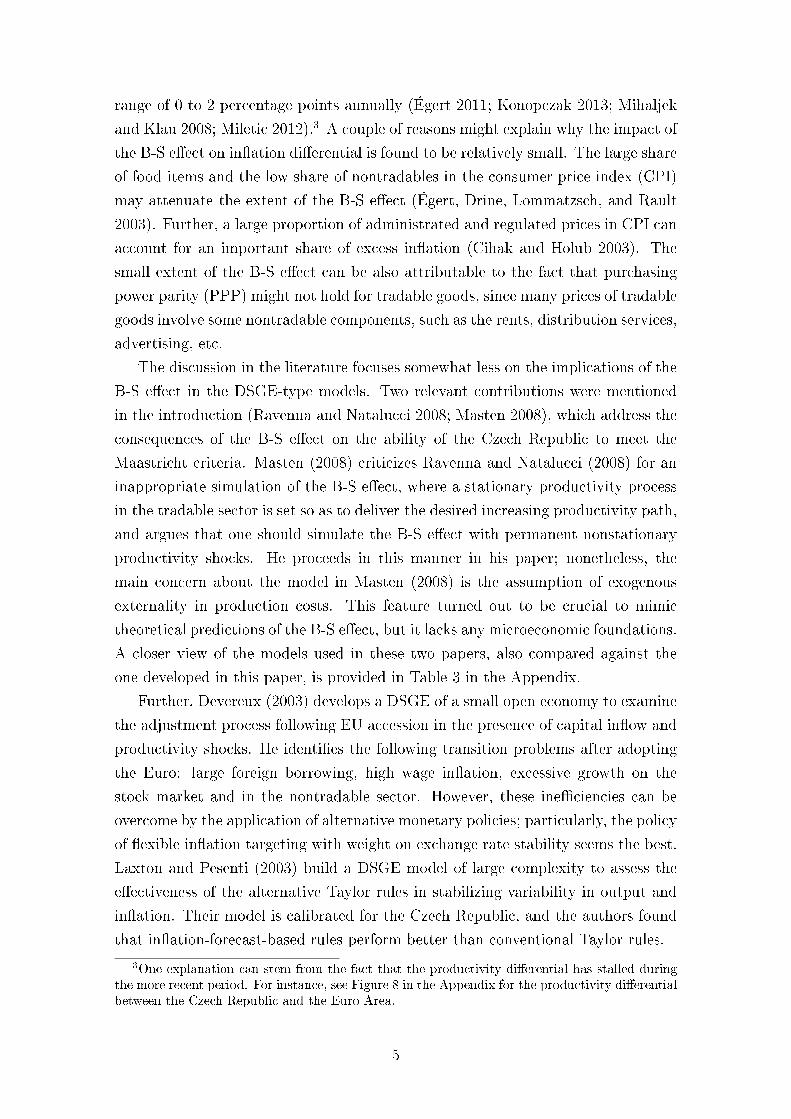
are composed from tradable, nontradable and foreign inputs. Tradable �rms are

allowed to use foreign inputs in their production. Notice that foreign goods im-

6

Figure 1: The Scheme of the Model

Consumption

Nontradable

investment

Exports

ImportsCapital

Labor

Tradable

firms

Tradable

investment

Rest of world

Households

tradable capital

Exports

Nontradable

firms

nontradable capital

plicitly enter nontradable production as well through capital accumulation. The

labor-augmenting productivity for tradable and nontradable �rms can di�er, which

enables the simulation of the B-S e�ect.

The value added of this model compared to Ravenna and Natalucci (2008) is

that it includes several more realistic features: i) the model is estimated on Czech

data using Bayesian techniques, ii) wages are set in staggered contracts, iii) habits

in consumption are allowed, iv) productivity growth can be permanent (balanced

growth path model), and v) the in�ation target can be non-zero. The features of the

model are shown in Figure 1, where the green parts depict the �ows in the tradable

sector, and the red parts represent the �ows in the nontradable sector.

3.1 Households

The economy is populated by a continuum of monopolistically competitive house-

holds, indexed by i ∈ [0, 1]. Each household supplies a di�erentiated labor service

to the �rms, and maximizes its lifetime utility function given by:

U(i) = E0

∞∑t=0

βt

{Dt log [Ct(i)− χcCt−1(i)]−l

[Lst(i)]1+ηL

1 + ηL

}, (1)

where β is a discount factor, χc is a consumption habit parameter, Dt is an ex-

ogenous preference shock, ηL is the inverse of the labor supply elasticity, l is the

parameter measuring relative disutility of labor supply, Ct(i) and Lst(i) are con-

7

sumption and labor supply of household i. Assuming perfect substitution between

hours worked in nontradable and tradable sectors, aggregate labor supply equals:

Lst = LNt + LHt (2)

Total consumption is a constant elasticity of substitution (CES) composite index

of nontradable and tradable consumption goods:

Ct =[(γn)

1ρN (CN,t)

ρN−1

ρN + (1− γn)1ρN (CT,t)

ρN−1

ρN

] ρNρN−1

, (3)

where 0 ≤ γn ≤ 1 is the share of nontradables in consumption, and ρN > 0 is

the elasticity of substitution between nontradable and tradable consumption goods.

The tradable consumption good is a CES composite of home and foreign tradable

goods:

CT,t =[(γh)

1ρH (CH,t)

ρH−1

ρH + (1− γh)1ρH (CF,t)

ρH−1

ρH

] ρHρH−1

, (4)

where 0 ≤ γh ≤ 1 is the share of domestic tradable goods in tradable consumption,

and ρH > 0 is the elasticity of substitution between domestic and foreign consump-

tion goods.4 The nontradable consumption good is an aggregate over a continuum

of di�erentiated goods:

CN,t =

1∫0

(CN,t)εN−1

εN (z)dz

εNεN−1

(5)

where the elasticity between nontradable good varieties εN > 1 and z ∈ [0, 1].

Based on the above preferences, it is possible to derive consumption-based price

indices:

Pt =[γn (PN,t)

1−ρN + (1− γn) (PH,t)1−ρN

] 11−ρN (6)

PN,t =

1∫0

(PN,t)1−εN (z)dz

1

1−εN

(7)

where Pt, and PN,t are the consumer price index (CPI), and the price index for

nontradable consumption goods. It is assumed that the price of tradable goods

is determined abroad, and the law of one price holds for tradable goods, and the

exchange rate pass-through is complete.5 So, the price for tradable goods is given4The posterior estimate of this elasticity turned out to be �at (see Figure 2), which suggests

that tradable aggregation may be simpli�ed, for instance using Cobb-Douglas speci�cation.5Ravenna and Natalucci (2008) also tried the speci�cation with local currency pricing for

foreign-produced goods. Its impact on the dynamics of aggregate variables following the B-Sshock was limited, which may be explained by the low share of foreign goods in tradable baskets.

8

as:

PH,t = ERtP∗t , (8)

where P ∗t is the exogenous foreign-currency price of tradable good, and ERt is the

nominal exchange rate, which is expressed as the value of foreign currency in units

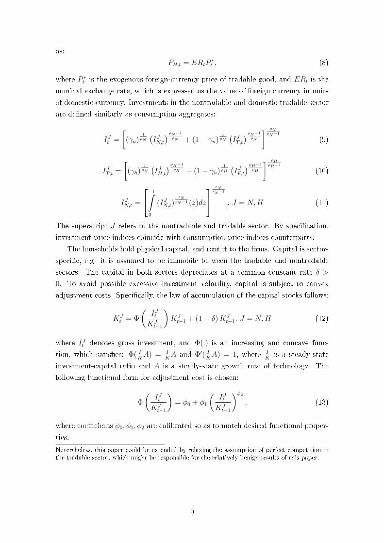
of domestic currency. Investments in the nontradable and domestic tradable sector

are de�ned similarly as consumption aggregates:

IJt =

[(γn)

1ρN

(IJN,t) ρN−1

ρN + (1− γn)1ρN

(IJT,t) ρN−1

ρN

] ρNρN−1

(9)

IJT,t =

[(γh)

1ρH

(IJH,t) ρH−1

ρH + (1− γh)1ρH

(IJF,t) ρH−1

ρH

] ρHρH−1

(10)

IJN,t =

1∫0

(IJN,t)εNεN−1 (z)dz

εNεN−1

, J = N,H (11)

The superscript J refers to the nontradable and tradable sector. By speci�cation,

investment price indices coincide with consumption price indices counterparts.

The households hold physical capital, and rent it to the �rms. Capital is sector-

speci�c, e.g. it is assumed to be immobile between the tradable and nontradable

sectors. The capital in both sectors depreciates at a common constant rate δ >

0. To avoid possible excessive investment volatility, capital is subject to convex

adjustment costs. Speci�cally, the law of accumulation of the capital stocks follows:

KJt = Φ

(IJtKJt−1

)KJt−1 + (1− δ)KJ

t−1, J = N,H (12)

where IJt denotes gross investment, and Φ(.) is an increasing and concave func-

tion, which satis�es: Φ( IKA) = I

KA and Φ′( I

KA) = 1, where I

Kis a steady-state

investment-capital ratio and A is a steady-state growth rate of technology. The

following functional form for adjustment cost is chosen:

Φ

(IJtKJt−1

)= φ0 + φ1

(IJtKJt−1

)φ2, (13)

where coe�cients φ0, φ1, φ2 are calibrated so as to match desired functional proper-

ties.

Nevertheless, this paper could be extended by relaxing the assumption of perfect competition inthe tradable sector, which might be responsible for the relatively benign results of this paper.

9

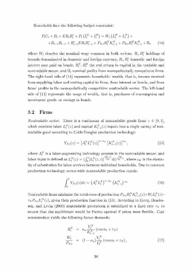
Households face the following budget constraint:

PtCt +Bt + ERtB∗t + Pt

(INt + IHt

)= Wt

(LHt + LNt

)+

+Rt−1Bt−1 +R∗t−1ERtB∗t−1 + PN,tR

Nt K

Nt−1 + PH,tR

Ht K

Ht−1 + Πt (14)

where Wt denotes the nominal wage common in both sectors; Bt, B∗t holdings of

bounds denominated in domestic and foreign currency, Rt, R∗t domestic and foreign

interest rate paid on bonds; RNt , R

Ht the real return to capital in the tradable and

nontradable sector, and Πt nominal pro�ts from monopolistically competitive �rms.

The right-hand side of (14) represents households' wealth, that is, income received

from supplying labor and renting capital to �rms, from interest on bonds, and from

�rms' pro�ts in the monopolistically competitive nontradable sector. The left-hand

side of (14) represents the usage of wealth, that is, purchases of consumption and

investment goods, or savings in bonds.

3.2 Firms

Nontradable sector. There is a continuum of nontradable goods �rms z ∈ [0, 1],

which combine labor LNt (z) and capital KNt−1(z) inputs into a single variety of non-

tradable good according to Cobb-Douglas production technology:

YN,t(z) =[ANt L

Nt (z)

]1−αn [KNt−1(z)

]αn, (15)

where ANt is a labor-augmenting technology process in the nontradable sector, and

labor input is de�ned as LNt (z) = (∫ 1

0[LNt (z, i)]

εW−1

εW di)εWεW−1 , where εW is the elastic-

ity of substitution for labor services between individual households. Due to common

production technology, sector-wide nontradable production equals:∫ 1

0

YN,t(z)dz =(ANt L

Nt

)1−αn (KNt−1)αn (16)

Nontradable �rms minimize the total costs of production PN,tRNt K

Nt−1(z)+WtL

Nt (z)−

τNPN,tYNt (z), given their production function in (15). According to Erceg, Hender-

son, and Levin (2000) nontradable production is subsidized at a �xed rate τN to

ensure that the equilibrium would be Pareto optimal if prices were �exible. Cost

minimization yields the following factor demands:

RNt = αn

Y Nt

KNt−1

(rmcnt + τN)

Wt

PN,t= (1− αn)

Y Nt

LNt(rmcnt + τN) , (17)

10

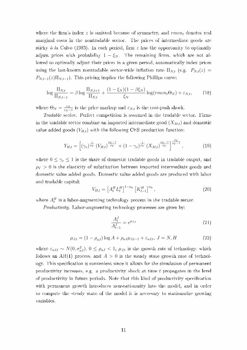
where the �rm's index z is omitted because of symmetry, and rmcnt denotes real

marginal costs in the nontradable sector. The prices of intermediate goods are

sticky à la Calvo (1983). In each period, �rm z has the opportunity to optimally

adjust prices with probability 1 − ξN . The remaining �rms, which are not al-

lowed to optimally adjust their prices in a given period, automatically index prices

using the last-known nontradable sector-wide in�ation rate ΠN,t (e.g. PN,t(z) =

PN,t−1(z)ΠN,t−1). This pricing implies the following Phillips curve:

logΠN,t

ΠN,t−1= β log

ΠN,t+1

ΠN,t

+(1− ξN)(1− βξN)

ξNlog(rmcntΘN) + εN,t, (18)

where ΘN = εNεN−1

is the price markup and εN,t is the cost-push shock.

Tradable sector. Perfect competition is assumed in the tradable sector. Firms

in the tradable sector combine an imported intermediate good (XM,t) and domestic

value added goods (VH,t) with the following CES production function:

YH,t =[(γv)

1ρV (VH,t)

ρV −1

ρV + (1− γv)1ρV (XM,t)

ρV −1

ρV

] ρVρV −1

, (19)

where 0 ≤ γv ≤ 1 is the share of domestic tradable goods in tradable output, and

ρV > 0 is the elasticity of substitution between imported intermediate goods and

domestic value added goods. Domestic value added goods are produced with labor

and tradable capital:

VH,t =[AHt L

Ht

]1−αh [KHt−1]αh , (20)

where AHt is a labor-augmenting technology process in the tradable sector.

Productivity. Labor-augmenting technology processes are given by:

AJtAJt−1

= eµJ,t (21)

µJ,t = (1− ρaJ) logA+ ρaJµJ,t−1 + εaJ,t, J = N,H (22)

where εaJ,t ∼ N(0, σ2aJ), 0 ≤ ρaJ < 1, µJ,t is the growth rate of technology, which

follows an AR(1) process, and A > 0 is the steady state growth rate of technol-

ogy. This speci�cation is convenient since it allows for the simulation of permanent

productivity increases, e.g. a productivity shock at time t propagates in the level

of productivity in future periods. Note that this kind of productivity speci�cation

with permanent growth introduces nonstationarity into the model, and in order

to compute the steady state of the model it is necessary to stationarize growing

variables.

11

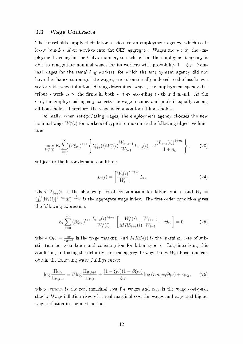
3.3 Wage Contracts

The households supply their labor services to an employment agency, which cost-

lessly bundles labor services into the CES aggregate. Wages are set by the em-

ployment agency in the Calvo manner, so each period the employment agency is

able to renegotiate nominal wages for its workers with probability 1 − ξW . Nom-

inal wages for the remaining workers, for which the employment agency did not

have the chance to renegotiate wages, are automatically indexed to the last-known

sector-wide wage in�ation. Having determined wages, the employment agency dis-

tributes workers to the �rms in both sectors according to their demand. At the

end, the employment agency collects the wage income, and pools it equally among

all households. Therefore, the wage is common for all households.

Formally, when renegotiating wages, the employment agency chooses the new

nominal wage W ∗t (i) for workers of type i to maximize the following objective func-

tion:

maxW ∗t (i)

Et

∞∑s=0

(βξW )t+s{λct+s(i)W

∗t (i)

Wt+s−1

Wt−1Lt+s(i)− l

(Lt+s(i))1+ηL

1 + ηL

}, (23)

subject to the labor demand condition:

Lt(i) =

[Wt(i)

Wt

]−εWLt, (24)

where λct+s(i) is the shadow price of consumption for labor type i, and Wt =

(∫ 1

0[Wt(i)]

1−εW di)1

1−εW is the aggregate wage index. The �rst order condition gives

the following expression:

Et

∞∑s=0

(βξW )t+sLt+s(i)

1+ηL

W ∗t (i)

[W ∗t (i)

MRSt+s(i)

Wt+s−1

Wt−1−ΘW

]= 0, (25)

where ΘW = εWεW−1

is the wage markup, and MRSt(i) is the marginal rate of sub-

stitution between labor and consumption for labor type i. Log-linearizing this

condition, and using the de�nition for the aggregate wage index Wt above, one can

obtain the following wage Phillips curve:

logΠW,t

ΠW,t−1= β log

ΠW,t+1

ΠW,t

+(1− ξW )(1− βξW )

ξWlog (rmcwtΘW ) + εW,t, (26)

where rmcwt is the real marginal cost for wages and εW,t is the wage cost-push

shock. Wage in�ation rises with real marginal cost for wages and expected higher

wage in�ation in the next period.

12

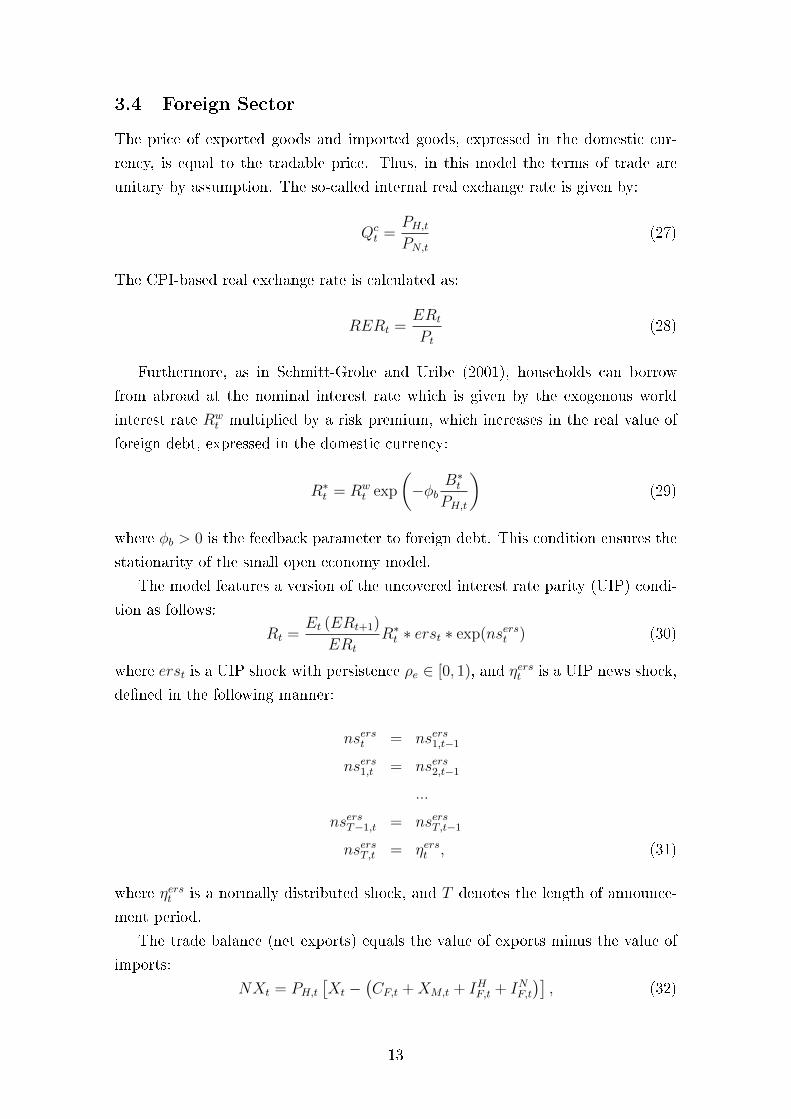
3.4 Foreign Sector

The price of exported goods and imported goods, expressed in the domestic cur-

rency, is equal to the tradable price. Thus, in this model the terms of trade are

unitary by assumption. The so-called internal real exchange rate is given by:

Qct =

PH,tPN,t

(27)

The CPI-based real exchange rate is calculated as:

RERt =ERt

Pt(28)

Furthermore, as in Schmitt-Grohe and Uribe (2001), households can borrow

from abroad at the nominal interest rate which is given by the exogenous world

interest rate Rwt multiplied by a risk premium, which increases in the real value of

foreign debt, expressed in the domestic currency:

R∗t = Rwt exp

(−φb

B∗tPH,t

)(29)

where φb > 0 is the feedback parameter to foreign debt. This condition ensures the

stationarity of the small open economy model.

The model features a version of the uncovered interest rate parity (UIP) condi-

tion as follows:

Rt =Et (ERt+1)

ERt

R∗t ∗ erst ∗ exp(nserst ) (30)

where erst is a UIP shock with persistence ρe ∈ [0, 1), and ηerst is a UIP news shock,

de�ned in the following manner:

nserst = nsers1,t−1

nsers1,t = nsers2,t−1

...

nsersT−1,t = nsersT,t−1

nsersT,t = ηerst , (31)

where ηerst is a normally distributed shock, and T denotes the length of announce-

ment period.

The trade balance (net exports) equals the value of exports minus the value of

imports:

NXt = PH,t[Xt −

(CF,t +XM,t + IHF,t + INF,t

)], (32)

13

where Xt are exports. In equilibrium trade is balanced.6 The net foreign debt law

of motion is given by the following relationship:

B∗t =ERt

ERt−1B∗t−1R

∗t−1 +NXt (33)

Modeling a small open economy, foreign variables � speci�cally foreign in�ation,

and the foreign gross nominal interest rate � are exogenously given:

Π∗tΠ

=

(Π∗t−1

Π

)ρpi∗exp(εpi∗t )

Rwt

R=

(Rwt−1

R

)ρrwexp(εrwt ) (34)

where Π∗t = P ∗t /P∗t−1, the steady states for foreign in�ation and world nominal

interest rates equal the steady states of their domestic counterparts, the ρ's from

[0, 1) measure the persistences of the exogenous processes, and ε's are normally

distributed shocks.

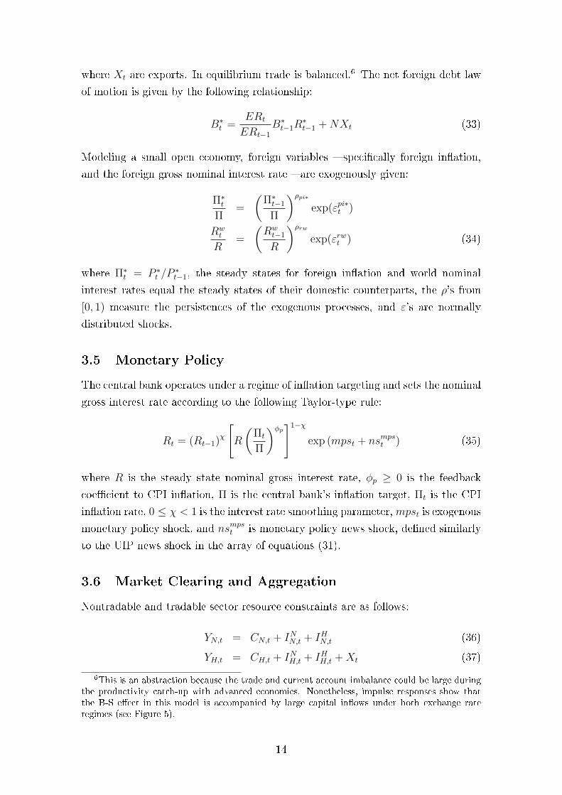
3.5 Monetary Policy

The central bank operates under a regime of in�ation targeting and sets the nominal

gross interest rate according to the following Taylor-type rule:

Rt = (Rt−1)χ

[R

(Πt

Π

)φp]1−χexp (mpst + nsmpst ) (35)

where R is the steady state nominal gross interest rate, φp ≥ 0 is the feedback

coe�cient to CPI in�ation, Π is the central bank's in�ation target, Πt is the CPI

in�ation rate, 0 ≤ χ < 1 is the interest rate smoothing parameter,mpst is exogenous

monetary policy shock, and nsmpst is monetary policy news shock, de�ned similarly

to the UIP news shock in the array of equations (31).

3.6 Market Clearing and Aggregation

Nontradable and tradable sector resource constraints are as follows:

YN,t = CN,t + INN,t + IHN,t (36)

YH,t = CH,t + INH,t + IHH,t +Xt (37)

6This is an abstraction because the trade and current account imbalance could be large duringthe productivity catch-up with advanced economies. Nonetheless, impulse responses show thatthe B-S e�ect in this model is accompanied by large capital in�ows under both exchange rateregimes (see Figure 5).

14

Aggregate output equals the value of nontradable and tradable output de�ated by

the CPI price:

Yt =PN,tPt

YN,t +PH,tPt

YH,t (38)

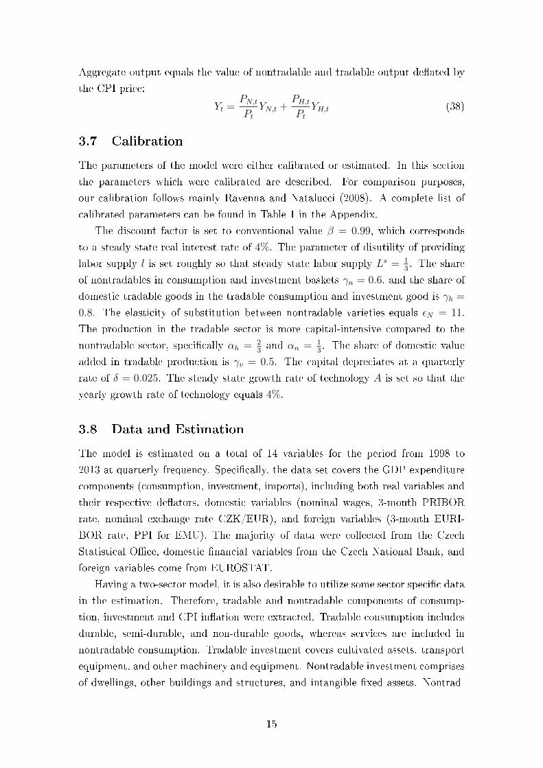
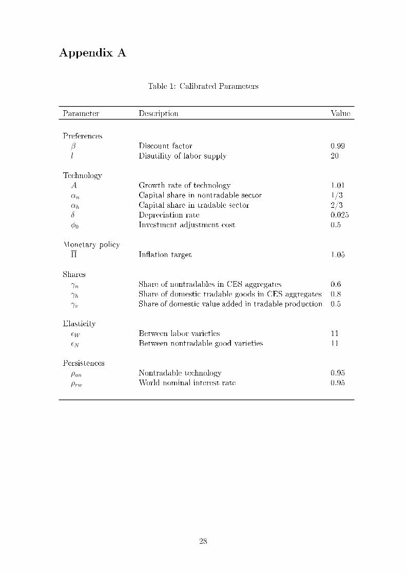
3.7 Calibration

The parameters of the model were either calibrated or estimated. In this section

the parameters which were calibrated are described. For comparison purposes,

our calibration follows mainly Ravenna and Natalucci (2008). A complete list of

calibrated parameters can be found in Table 1 in the Appendix.

The discount factor is set to conventional value β = 0.99, which corresponds

to a steady state real interest rate of 4%. The parameter of disutility of providing

labor supply l is set roughly so that steady state labor supply Ls = 13. The share

of nontradables in consumption and investment baskets γn = 0.6, and the share of

domestic tradable goods in the tradable consumption and investment good is γh =

0.8. The elasticity of substitution between nontradable varieties equals εN = 11.

The production in the tradable sector is more capital-intensive compared to the

nontradable sector, speci�cally αh = 23and αn = 1

3. The share of domestic value

added in tradable production is γv = 0.5. The capital depreciates at a quarterly

rate of δ = 0.025. The steady state growth rate of technology A is set so that the

yearly growth rate of technology equals 4%.

3.8 Data and Estimation

The model is estimated on a total of 14 variables for the period from 1998 to

2013 at quarterly frequency. Speci�cally, the data set covers the GDP expenditure

components (consumption, investment, imports), including both real variables and

their respective de�ators, domestic variables (nominal wages, 3-month PRIBOR

rate, nominal exchange rate CZK/EUR), and foreign variables (3-month EURI-

BOR rate, PPI for EMU). The majority of data were collected from the Czech

Statistical O�ce, domestic �nancial variables from the Czech National Bank, and

foreign variables come from EUROSTAT.

Having a two-sector model, it is also desirable to utilize some sector speci�c data

in the estimation. Therefore, tradable and nontradable components of consump-

tion, investment and CPI in�ation were extracted. Tradable consumption includes

durable, semi-durable, and non-durable goods, whereas services are included in

nontradable consumption. Tradable investment covers cultivated assets, transport

equipment, and other machinery and equipment. Nontradable investment comprises

of dwellings, other buildings and structures, and intangible �xed assets. Nontrad-

15

able in�ation covers services, whereas tradable in�ation follows price changes in

food, fuel and other tradable goods.

In the estimation, a stationary version of the model is used, e.g. productivity

growth is temporary, and the in�ation target is set to zero. Input data are detrended

with an HP-�lter, which means that only the business cycle information is retained.

Observed data are linked to the model variables through a block of measurement

equations. In these equations, the model variables are the sum of observed data

and the measurement error. The standard deviation of speci�c measurement error

is calibrated at roughly one fourth of the standard deviation of the corresponding

observed data.

The prior distributions for the estimated parameters were chosen as follows.

For parameters constrained on the interval 〈0, 1〉, the beta distribution is used.

This concerns, for example, the elasticity of substitution between nontradable and

tradable goods in the CES aggregates ρN , which re�ects the idea that nontradable

and tradable goods are likely to be complements. The standard errors of shocks

have priors from inverse gamma distributions. Also, the feedback parameter to

foreign debt φb has prior from inverse gamma distribution, since it attains rather

low values. For remaining parameters, the priors take form of normal distribution.

Estimation itself is carried out in the Dynare Toolbox.7 The prior distributions of

a subset of the model parameters get combined with the likelihood function based on

the observed data. This results in posterior distributions for particular parameters.

First, the Dynare is instructed to use numerical optimization techniques to search

for the posterior modes of the parameters. Next, the draws from the posterior

distributions around these modes are taken using the random walk Metropolis-

Hastings (MH) algorithm. To ensure that convergence of the posterior simulations

has been achieved, three parallel MH blocks are run, with a length of 200,000

draws. The �rst half of the draws get thrown away as a burn-in. Both simulations

result in average acceptance rates of approximately 26%. Figures 2 through 4 in

the Appendix show the comparison of the prior/posterior distributions and the

results of the multivariate convergence diagnostic test. During the estimation, two

parameters � persistences of nontradable technology and world nominal interest rate

� indicated the presence of computational problems, thus they were removed from

the estimation, and their values were calibrated.

A comparison of the prior and posterior distributions for the estimated parame-

ters can be found in Table 2 in the Appendix. A high posterior mean of the inverse

elasticity of labor supply ηL = 4.4 suggests low elasticity of labor supply in the

Czech Republic. The estimated value of habit parameter χc = 0.6 implies that the

households care about smoothing their consumption over time. Observed data fa-7Matlab-based toolbox, for further information see www.dynare.org.

16

vored the posterior mean for the elasticity of substitution between nontradable and

tradable goods in the CES aggregates ρN = 0.76; however, there was little infor-

mation in the data for the elasticities of substitution between domestic and foreign

goods (ρH , ρV ), for which prior and posterior means are roughly the same. Calvo

probabilities in the nontradable sector and wage setting (ξN , ξL) turned out to be

rather low, showing that nontradable �rms adjust their prices on average every two

quarters (∼ 1/(1 − 0.4)) and that wage contracts are rather �exible, renewed on

average every quarter. The interest rate smoothing parameter χ = 0.4 achieves

slightly lower value than its prior mean. The feedback coe�cient to the in�ation

gap is rather strong, with posterior mean φp = 2.7. The feedback parameter to

foreign debt achieves φb = 0.002, which is lower than its prior mean. Posterior

means for persistences in autoregressive processes attain values between 0.4 to 0.8,

with the smallest one associated with the UIP shock and the largest one with the

demand shock. The estimates of the standard deviations of structural shocks point

to the fact that productivity shock in the tradable sector is the most volatile.

3.9 Steady State

Given the calibrated and estimated parameters of the model, the steady state of the

model is computed. Estimated parameters are evaluated at their posterior means.

Since the model involves several price levels, one price level is taken as a numeraire

and the remaining prices are expressed with respect to this chosen numeraire. Fur-

ther, as was pointed out earlier, the presence of permanent productivity shocks

makes the model nonstationary, and consequently it is not possible to directly com-

pute its steady state. Therefore, one needs to perform additional transformations �

a detrending of growing variables � in order to solve for the steady state. The de-

trending of the variables is as follows. Except for the labor supply, real variables are

divided by the level of the labor-augmenting technology process in the nontradable

sector, e.g. X̃t = Xt/ANt , where X̃t is the transformed or detrended variable. The

selection of technology process for detrending is arbitrary, but in the simulations

of the B-S e�ect the productivity growth in the tradable sector is faster than in

the nontradable sector, and to judge directly the e�ects of excessive growth in the

tradable sector on real variables, it is preferable to express real variables with re-

spect to the technology process in the nontradable sector. Another issue here is that

the detrending of the shadow price of consumption λct (or the Lagrange multiplier

associated with the budget constraint) is somewhat more complicated because a

transformed version of this variable is given by the original one multiplied both by

the numeraire price level and by the technology process in the nontradable sector.

Afterwards, all optimality conditions are rewritten in detrended variables. Using

17

substitutions within the system of steady-state versions of the optimality condi-

tions, it is possible to numerically compute steady-state values for all the model

variables. Having computed the steady state, the system of optimality conditions

is log-linearized around the steady state and solved using the IRIS toolbox.8

4 The Results

In this section several simulations are carried out. Firstly, impulse responses to

productivity shock in the tradable sector are inspected, both under �exible- and

�xed-exchange-rate regimes. Secondly, transition from �exible to �xed exchange

rate is modeled on the background of the B-S e�ect. Thirdly, the issue raised by

Masten (2008) about the appropriate simulation of the B-S e�ect is brie�y ad-

dressed. Lastly, the robustness of the results is checked.

4.1 The B-S E�ect under Flexible and Fixed Exchange Rate

Regime

For the purposes of comparison, the B-S e�ect is simulated as in Ravenna and

Natalucci (2008), assuming a 30% gradual productivity increase in the tradable

sector over 10 years. This growth is also relative to the foreign economy, and

thus can be re-interpreted as excess relative productivity growth against the foreign

economy (Euro Area). At the beginning of the simulation it is assumed that the

economy is in its steady state. Impulse responses to such calibrated productivity

shocks are depicted in Figure 5 in the Appendix. Blue lines represent the simulation

with a �xed exchange rate, and red lines in the case of a �exible exchange rate. In

the simulation with a �xed exchange rate, the monetary policy rule is turned o�,

and the domestic interest rate equals the foreign interest rate, as de�ned in equation

29.

Except for the nominal exchange rate, it does not matter what kind of exchange

rate regime is adopted in the economy, �exible or �xed, since the impulse responses

overlap in the long run. Under the �exible-exchange-rate regime, the nominal ex-

change rate appreciates by about 6% in the long run, as productivity grows by 30%

in the tradable sector. However, in the short run, the dynamics di�er between these

two exchange rate regimes. With a �xed-exchange-rate regime, there are stronger

in�ationary pressures, with CPI in�ation rising on impact by approximately 7 per-

centage points in annualized terms. This in�ation arises solely from the nontradable

sector because tradable in�ation is linked to foreign tradable in�ation, which is un-8IRIS is a MATLAB toolbox for macroeconomic modeling and forecasting, developed by Bene²

(2014). For further information see www.iris-toolbox.com.

18

a�ected by the shock to domestic tradable productivity. Note that under a �xed

exchange rate the in�ationary pressures cannot be mitigated with the monetary pol-

icy by de�nition. With a �exible exchange rate, in�ation drops on impact, which is

given by an initial appreciation of the nominal exchange rate. There are still some

in�ationary pressures coming from the nontradable sector, albeit notably smaller

compared to the �xed-exchange-rate regime. The CPI-based real exchange rate

appreciates approximately 6% in the long run under both exchange rate regimes.

Comparing the two exchange rate regimes, there is an obvious trade-o� be-

tween nominal exchange rate appreciation and in�ationary pressures in response

to the productivity shock in the tradable sector. Either there are higher in�ation-

ary pressures with a �xed-exchange-rate regime, or higher nominal exchange rate

appreciation in the case of a �exible-exchange-rate regime.

Qualitatively, these results resemble those of Ravenna and Natalucci (2008),

but the extent of exchange rate appreciation in this paper is found to be somewhat

smaller. Some di�erence might be attributable to di�erent calibration and structure

of their model (for details see Table 3 in the Appendix). Overall, the model mimics

the theoretical predictions of the B-S e�ect well, captured by appreciating exchange

rates and/or rising in�ationary pressures in response to growing productivity in the

tradable sector.

4.2 Transition from Flexible to Fixed Exchange Rate

Currently, the Czech economy has a �oating exchange rate, which will switch to

a �xed exchange rate after the adoption of the Euro. Therefore, it is interesting

to inspect what is likely to happen to the economy before, during and after the

adoption of the Euro on the back of the productivity catch-up process to the rest

of Europe.

Performing such a simulation is not straightforward, since after the switch, a

di�erent set of equations describe the economy. Speci�cally, monetary policy loses

its power to control the domestic interest rate, and the domestic interest rate equals

the foreign interest rate (including a risk premium). To allow for such a change in

the model, one possible way is to adjust a�ected equations with desired calibrated

shocks. Firstly, the UIP shocks (in Eq. 30) are calibrated so that the nominal

exchange rate remains �xed after the switch. Secondly, after the switch to a �xed

exchange regime, monetary policy shocks to the monetary policy rule (in Eq. 35)

are calibrated so as to make the domestic interest rate equal to the foreign interest

rate. The calibration of monetary policy shocks is somewhat tricky, since the do-

mestic interest rate is an endogenous variable, whose trajectory is unknown prior

to the simulation. Hence, initially, the trajectory of the domestic interest rate is

19

conditionally set after the switch to its steady state level. A preliminary simulation

is run, and the di�erence between the trajectories of domestic and foreign interest

rates is computed. In the next iteration, the trajectory of the domestic interest

rate is set according to the last known trajectory of the foreign interest rate. The

iterations continue until the di�erence between the trajectories of the domestic and

foreign interest rates are minimized. This way one searches for desired monetary

policy shocks that would deliver a state in which the domestic interest rate equals

the foreign interest rate, e.g. the condition valid in a �xed exchange rate regime.

Again, as in the previous section, a 30% gradual productivity increase in the

tradable sector over 10 years is assumed, but at some point the transition from

a �exible to a �xed exchange rate occurs. What is relevant for the dynamics in

the transition is the level of nominal exchange rate which will be valid after the

adoption of the Euro, e.g. what the conversion rate is that will �x the Czech

crown against the Euro. Basically, the country might �x its exchange rate at a

depreciated, appreciated or consistent level as compared to the previous level of

nominal exchange rate in the �oating regime. Furthermore, the story is di�erent

when transition to a �xed exchange rate regime happens during episodes of higher

or lower productivity gains. What also matters for the transition is whether the

conversion rate is preannounced to the public or not. All these issues are addressed

in the following text.

In Figure 6 in the Appendix the trajectories of selected variables are shown for

the transition from a �exible to a �xed exchange rate. The switch occurs in the 8th

quarter, and the level of �xed exchange rate is preannounced 4 quarters ahead of

the switch, which is highlighted by a shaded area. Gold trajectories are for the case

of a �exible exchange rate, that is, without the switch to a �xed exchange rate. Red

trajectories are for the case when the �xed exchange rate is set to the last value of

the �exible exchange rate. Black/blue trajectories are for depreciated/appreciated

�xed exchange rates by 1 percentage point compared to the case when the exchange

rate would remain �exible at the time of the switch. Comparing the results, the

highest in�ation pressures occur in the case of a depreciated �xed exchange rate,

as a large proportion of in�ation is imported from abroad through a depreciated

currency. Across di�erent conversion rates the dynamics of real variables, such as

output or consumption, remain largely intact, especially in the long run. Soon after

the switch to a �xed exchange rate regime, CPI in�ation reaches similar trajectories

for all cases. In the "red" case, which represents the �x at the last value of the

�exible exchange rate, CPI in�ation in the �rst year after the switch is on average

approximately 0.4 percentage points higher compared to the case of the �exible

exchange rate.

The timing of the transition from a �exible to a �xed exchange rate regime is

20

also of key importance. The comparison of two di�erent timings of transition is

shown in Figure 7 in the Appendix. Red lines depict the simulation when a �xed

exchange rate is adopted in period 8, when the average productivity growth of a

tradable sector is approximately 4% annually. Blue lines represent the case where a

�xed exchange rate is adopted in period 20, with slower productivity growth in the

tradable sector reaching around 1% annually. Comparing these two simulations,

early adoption of the Euro brings additional in�ation costs, amounting on average

to 0.3 percentage points higher CPI in�ation when compared to the alternative case

of a later transition. However, the timing of the transition does not matter for the

in�ationary pressures prior to the adoption of the Euro. Also, the dynamics of real

variables are almost una�ected by di�erent timing of the transition. The results

suggest that a country should consider during what stage of the productivity catch-

up process it should enter the EA, since early transition might be associated initially

with higher in�ation, rising by some 0.4 percentage points in the �rst year after the

adoption of the Euro. These higher in�ation pressures do not seem large, but one

should bear in mind that they cannot be mitigated against by domestic monetary

policy, since its power is lost in the �xed exchange rate regime.

To be more realistic, this timing exercise is also repeated using a labor pro-

ductivity di�erential as a proxy for actual productivity improvement between the

Czech Republic and the Euro Area, depicted in Figure 8 over the time periods

of 2000�2015. Real labor productivity per hour worked is extracted from the

Eurostat database (variable namq_10_lp_ulc), and seasonally adjusted by the

Tramo/Seats method. To eliminate short-run �uctuations, the productivity di�er-

ential is smoothed with the H-P �lter, with the smoothing parameter set to 5. For

comparison, this productivity di�erential is also plotted against the autoregressive

process for the tradable/nontradable technology wedge used in previous simulations.

Current data show that productivity improved in the Czech Republic relative to the

Euro Area by more than 30% between 2000 and 2008, but from the Great Recession

the productivity catch-up process has stalled. Figure 9 shows di�erent timing of the

transition from a �exible to a �xed exchange rate regime on the background of a

current productivity di�erential. Early transition occurs in the 2nd quarter of 2004

(to re�ect the entry of the Czech Republic into the European Union), whereas later

transition is at the beginning of 2009 (chosen as the time when Slovakia entered

the Euro Area). Comparing these two timings, hypothetical early adoption of the

Euro brings additional in�ationary costs, reaching on average 0.4 percentage points

higher CPI in�ation when compared to the later transition. Initially, in�ation rises

by 0.6 percentage points in the �rst year after early adoption of the Euro. In the

event that the exchange rate remains �exible until the later transition, the nominal

exchange rate appreciation driven by the B-S e�ect is stronger by approximately 2

21

percentage points compared to the case of early transition.

The country might opt to adopt a single currency by surprise. Such simulation

is available in Figure 10 in the Appendix, with red/blue lines showing the unex-

pected/expected switch to a �xed exchange rate regime. Further, it is arbitrarily

assumed that a depreciated �xed exchange rate by 1 percentage point is going to

be adopted, compared to the case where the exchange rate would remain �exible at

the time of the switch. Inspecting the results, the adoption of the Euro by surprise

does not seem to be preferable, since it is associated with higher in�ation at the

time of the switch.

4.3 Masten's Critique

In this section, the issue of proper simulation of the B-S e�ect raised by Masten

(2008) is brie�y addressed. Masten (2008) criticizes Ravenna and Natalucci (2008)

for inappropriate simulation of the B-S e�ect, saying that: "..real appreciation in

response to their simulation of BS e�ect is not an equilibrium process. On the

contrary, it is a consequence of a large deviation from the actual equilibrium pro-

ductivity level of the economy leading to model dynamics that appear empirically

unlikely." Further in his paper he repeats his critique in other words: "Natalucci

and Ravenna (2002) construct the BS experiment by pushing a stationary process

of tradable productivity very far away from equilibrium with a sequence of positive

productivity shocks for 40 quarters. This means that at the time when tradable pro-

ductivity is supposed to reach a new steady state value (in 10 years) is in fact the

farthest away from the steady state. The tradable productivity increase is thus not

constructed as an equilibrium-driving process." As a remedy to this issue Masten

(2008) proposes using permanent sector-speci�c shocks so as to properly simulate

the B-S e�ect as an equilibrium-driving process.

The model in this paper allows using permanent sector-speci�c productivity

shocks in the simulation of the B-S e�ect. Nonetheless, both the simulation of the

B-S e�ect with permanent shocks and the simulation with temporary shocks in the

manner of Ravenna and Natalucci (2008) were tried and lead to the same results.

For instance, the impulse responses shown in Figure 5 in the Appendix are identical

for the simulation with permanent productivity shocks and for the simulation with

temporary shocks, where a stationary productivity process in the tradable sector is

exogenized so to match desired productivity path. In light of these results, Masten's

critique of the paper by Ravenna and Natalucci (2008) seems to be unjusti�ed.

Concerning exchange rate appreciation, driven by the B-S e�ect, in Masten

(2008) it is only present when the model assumes exogenous externality in the

production costs. In this paper such externality is not considered, and the simulation

22

of the B-S e�ect results in exchange rate appreciation. Nonetheless, the conclusions

of both papers are similar that the B-S e�ect is not an issue for the Czech Republic

to ful�ll the in�ation and nominal exchange rate criteria.

4.4 Robustness

The results were checked against several alternative assumptions. Concerning the

parameters of the model, perhaps the largest sensitivity of the results is found with

respect to the elasticity of substitution between nontradable and tradable goods

in the CES aggregates and the degree of price rigidity in the nontradable sector.

Therefore, in this section these two parameters are varied to check the implications

for the B-S e�ect.

Blue lines in Figures 11�12 in the Appendix show the simulations of the B-S e�ect

assuming lower elasticity of substitution between nontradable and tradable goods

ρN = 0.5, compared to the baseline in red lines with ρN = 0.76. Black lines in the

same �gures depict the simulations of the B-S e�ect assuming higher price rigidity

in the nontradable sector ξN = 0.8, compared to the baseline where ξN = 0.4.

Alternative calibrations of these two parameters are adopted from Ravenna and

Natalucci (2008). Gold lines represent the combination of both lower elasticity of

substitution between nontradable and tradable goods and higher price rigidity in

the nontradable sector. Impulse responses in Figure 11 are in the case of a �exible

exchange rate, and Figure 12 in case of a �xed exchange rate.

Lower elasticity of substitution between nontradable and tradable goods makes

the B-S e�ect under a �exible exchange rate regime more pronounced through nom-

inal exchange rate appreciation. The nominal exchange rate appreciates by almost

8% over ten years; however, it does not breach the limit imposed by the ERM

II mechanism. The e�ect on CPI in�ation is similar to the baseline. There is a

shift in the production patterns, with more production occurring in the nontrad-

able sector in comparison to the baseline, which is given by di�erent preferences

over nontradable and tradable goods in the consumption/investment baskets. The

B-S e�ect under a �exible exchange rate with a higher degree of price rigidity in the

nontradable sector resembles the baseline; however, some di�erences are notable.

The nominal exchange rate appreciates slightly more in the long run. Further,

the response of nontradable in�ation is initially below the baseline, but thereafter

persistently higher in the long run.

The B-S e�ect under a �xed exchange rate regime with lower elasticity of sub-

stitution between nontradable and tradable goods is more ampli�ed through CPI

in�ation, which reaches 13% on impact in annualized terms, compared to the 7%

initial increase in the baseline. The impulse responses of real variables, such as out-

23

put, consumption and real exchange rate, are similar to the case of �exible exchange

rate in the long run. The B-S e�ect under a �xed exchange rate regime with a higher

degree of price rigidity in the nontradable sector becomes less pronounced through

the response of the CPI in�ation. The initial response is roughly half compared to

the baseline, but the response is longer-lived over the �rst two years.

Interestingly, the alternative calibrations do not change signi�cantly the main

conclusions of this paper concerning the additional in�ation costs of early adoption

of the Euro. The same simulations as in Figure 7 in the Appendix were replicated for

alternative values of the elasticity of substitution between nontradable and tradable

goods and the degree of price rigidity in the nontradable sector. In these simulations,

early adoption of the Euro brings additional in�ation costs, amounting to on average

0.2 percentage-point higher CPI in�ation when compared to the alternative case of

later transition. This is slightly less compared to the baseline, with on average 0.3

percentage-point higher CPI in�ation over the period of early and later transition.

5 Conclusion

The B-S e�ect implies that highly productive countries have higher in�ation and

appreciating real exchange rates because of larger productivity growth di�erentials

between tradable and nontradable sectors relative to advanced economies. This is

also particularly important for the Czech Republic, in which a catch-up process with

advanced European countries is still ongoing. At some point, the Czech Republic

is obliged to adopt the Euro as a single currency. Before adopting the Euro the

Maastricht convergence criteria have to be ful�lled, imposing among others limits on

in�ation and nominal exchange rate �uctuations. An ongoing convergence process

or the presence of the B-S e�ect might restrain a country from complying with these

Maastricht criteria. Therefore, the main goal of this paper is to answer the question

whether the B-S e�ect could be an issue for the Czech Republic in its ability to

meet the Maastricht criteria.

For this purpose, I build a two-sector DSGE model of a small open economy,

estimated for the Czech Republic using Bayesian techniques. The structure of the

model is close to the one in Ravenna and Natalucci (2008), but is extended by several

more realistic features, including staggered wages, consumption habits, permanent

productivity growth, and a non-zero in�ation target. The prices are sticky in the

nontradable sector, whereas in the tradable sector �exible prices are assumed and

purchasing power parity holds for tradable goods.

The simulations from the model point to the fact that the B-S e�ect does not

pose a problem for the Czech Republic in meeting the Maastricht convergence cri-

teria before adopting the Euro. The costs of early adoption of the Euro are not so

24

large in terms of additional in�ationary pressures, which materialize after the adop-

tion of the single currency. More speci�cally, early transition is associated with

initially higher in�ation, rising by some 0.4 percentage points in the �rst year after

the adoption of the Euro. Also, nominal exchange rate appreciation, driven by the

B-S e�ect, does not breach the limit imposed by the ERM II mechanism. In the

baseline version of the model, the nominal exchange rate appreciates by about 6%

in the long run, as productivity increases by 30%.

This paper can be extended in several ways. For example, the model can be

improved by relaxing some of its underlying assumptions, such as a perfectly com-

petitive tradable sector and balanced trade in the equilibrium. Further, one can

extend its structure to include the �scal block in order to study the implications of

the B-S e�ect on the Maastricht �scal criteria, which impose the limits on govern-

ment budget balance and debt. Another interesting extension would be to search

for optimal monetary policy, which would minimize the costs of the B-S e�ect before

the adoption of the Euro.

25

References

Balassa, B. (1964). The Purchasing-Power Parity Doctrine: A Reappraisal. Jour-

nal of Political Economy 72, 584�596.

Bene², J. (2014). Iris toolbox reference manual. Ver. 2014-04-02.

Calvo, G. A. (1983). Staggered prices in a utility-maximizing framework. Journal

of Monetary Economics 12 (3), 383�398.

Cihak, M. and T. Holub (2003). Price Convergence: What Can the Balassa-

Samuelson Model Tell Us? Czech Journal of Economics and Finance (Finance

a úv¥r) 53 (7-8), 334�355.

Devereux, M. B. (2003). A Macroeconomic Analysis of EU Accession under Alter-

native Monetary Policies. Journal of Common Market Studies 41 (5), 941�964.

Erceg, C. J., D. W. Henderson, and A. T. Levin (2000). Optimal Monetary

Policy with Staggered Wage and Price Contracts. Journal of Monetary Eco-

nomics 46 (2), 281�313.

Égert, B. (2011). Catching-up and in�ation in europe: Balassa-samuelson, engel's

law and other culprits. Economic Systems 35 (2), 208�229.

Égert, B., I. Drine, K. Lommatzsch, and C. Rault (2003). The Balassa-Samuelson

E�ect in Central and Eastern Europe: Myth or Reality? Journal of Compar-

ative Economics 31 (3), 552�572.

Égert, B., L. Halpern, and R. MacDonald (2006). Equilibrium exchange rates

in transition economies: Taking stock of the issues. Journal of Economic

Surveys 20 (2), 257�324.

Ghironi, F. and M. J. Melitz (2005). International Trade and Macroeco-

nomic Dynamics with Heterogeneous Firms. The Quarterly Journal of Eco-

nomics 120 (3), 865�915.

Konopczak, K. (2013). The Balassa-Samuelson e�ect and the channels of its ab-

sorption in the Central and Eastern European Countries. National Bank of

Poland Working Papers 163, National Bank of Poland, Economic Institute.

Laxton, D. and P. Pesenti (2003). Monetary Rules for Small, Open, Emerging

Economies. Journal of Monetary Economics 50 (5), 1109�1146.

Lipinska, A. (2008). The Maastricht Convergence Criteria and Optimal Mone-

tary Policy for the EMU Accession Countries. Working Paper Series 0896,

European Central Bank.

Masten, I. (2008). Optimal Monetary Policy with Balassa-Samuelson-type Pro-

ductivity Shocks. Journal of Comparative Economics 36 (1), 120�141.

26

Mihaljek, D. and M. Klau (2004). The Balassa�Samuelson E�ect in Central Eu-

rope: A Disaggregated Analysis. Comparative Economic Studies 46 (1), 63�94.

Mihaljek, D. and M. Klau (2008). Catching-up and in�ation in transition

economies: the Balassa-Samuelson e�ect revisited. BIS Working Papers 270,

Bank for International Settlements.

Miletic, M. (2012). Estimating the Impact of the Balassa-Samuelson E�ect in

Central and Eastern European Countries: A Revised Analysis of Panel Data

Cointegration Tests. Working papers 22, National Bank of Serbia.

Rabanal, P. (2009). In�ation Di�erentials between Spain and the EMU: A DSGE

Perspective. Journal of Money, Credit and Banking 41 (6), 1141�1166.

Ravenna, F. and F. M. Natalucci (2008). Monetary Policy Choices in Emerg-

ing Market Economies: The Case of High Productivity Growth. Journal of

Money, Credit and Banking 40 (2-3), 243�271.

Sadeq, T. (2008). Bayesian estimation of a dsge model and convergence dynam-

ics analysis for central europe transition economies. Université d'Evry Val

d'Essonne, mimeo.

Samuelson, P. A. (1964). Theoretical Notes on Trade Problems. Review of Eco-

nomics and Statistics 46, 145�154.

Schmitt-Grohe, S. and M. Uribe (2001). Stabilization Policy and the Costs of

Dollarization. Journal of Money, Credit and Banking 33 (2), 482�509.

27

Appendix A

Table 1: Calibrated Parameters

Parameter Description Value

Preferencesβ Discount factor 0.99l Disutility of labor supply 20

TechnologyA Growth rate of technology 1.01αn Capital share in nontradable sector 1/3αh Capital share in tradable sector 2/3δ Depreciation rate 0.025φ0 Investment adjustment cost 0.5

Monetary policyΠ In�ation target 1.05

Sharesγn Share of nontradables in CES aggregates 0.6γh Share of domestic tradable goods in CES aggregates 0.8γv Share of domestic value added in tradable production 0.5

ElasticityεW Between labor varieties 11εN Between nontradable good varieties 11

Persistencesρan Nontradable technology 0.95ρrw World nominal interest rate 0.95

28

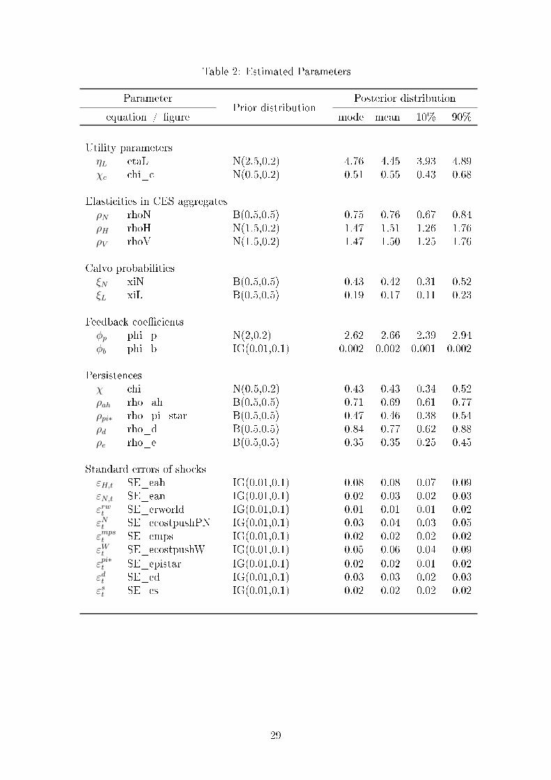
Table 2: Estimated Parameters

ParameterPrior distribution

Posterior distribution

equation / �gure mode mean 10% 90%

Utility parametersηL etaL N(2.5,0.2) 4.76 4.45 3.93 4.89χc chi_c N(0.5,0.2) 0.51 0.55 0.43 0.68

Elasticities in CES aggregatesρN rhoN B(0.5,0.5) 0.75 0.76 0.67 0.84ρH rhoH N(1.5,0.2) 1.47 1.51 1.26 1.76ρV rhoV N(1.5,0.2) 1.47 1.50 1.25 1.76

Calvo probabilitiesξN xiN B(0.5,0.5) 0.43 0.42 0.31 0.52ξL xiL B(0.5,0.5) 0.19 0.17 0.11 0.23

Feedback coe�cientsφp phi_p N(2,0.2) 2.62 2.66 2.39 2.94φb phi_b IG(0.01,0.1) 0.002 0.002 0.001 0.002

Persistencesχ chi N(0.5,0.2) 0.43 0.43 0.34 0.52ρah rho_ah B(0.5,0.5) 0.71 0.69 0.61 0.77ρpi∗ rho_pi_star B(0.5,0.5) 0.47 0.46 0.38 0.54ρd rho_d B(0.5,0.5) 0.84 0.77 0.62 0.88ρe rho_e B(0.5,0.5) 0.35 0.35 0.25 0.45

Standard errors of shocksεH,t SE_eah IG(0.01,0.1) 0.08 0.08 0.07 0.09εN,t SE_ean IG(0.01,0.1) 0.02 0.03 0.02 0.03εrwt SE_erworld IG(0.01,0.1) 0.01 0.01 0.01 0.02εNt SE_ecostpushPN IG(0.01,0.1) 0.03 0.04 0.03 0.05εmpst SE_emps IG(0.01,0.1) 0.02 0.02 0.02 0.02εWt SE_ecostpushW IG(0.01,0.1) 0.05 0.06 0.04 0.09εpi∗t SE_epistar IG(0.01,0.1) 0.02 0.02 0.01 0.02εdt SE_ed IG(0.01,0.1) 0.03 0.03 0.02 0.03εst SE_es IG(0.01,0.1) 0.02 0.02 0.02 0.02

29

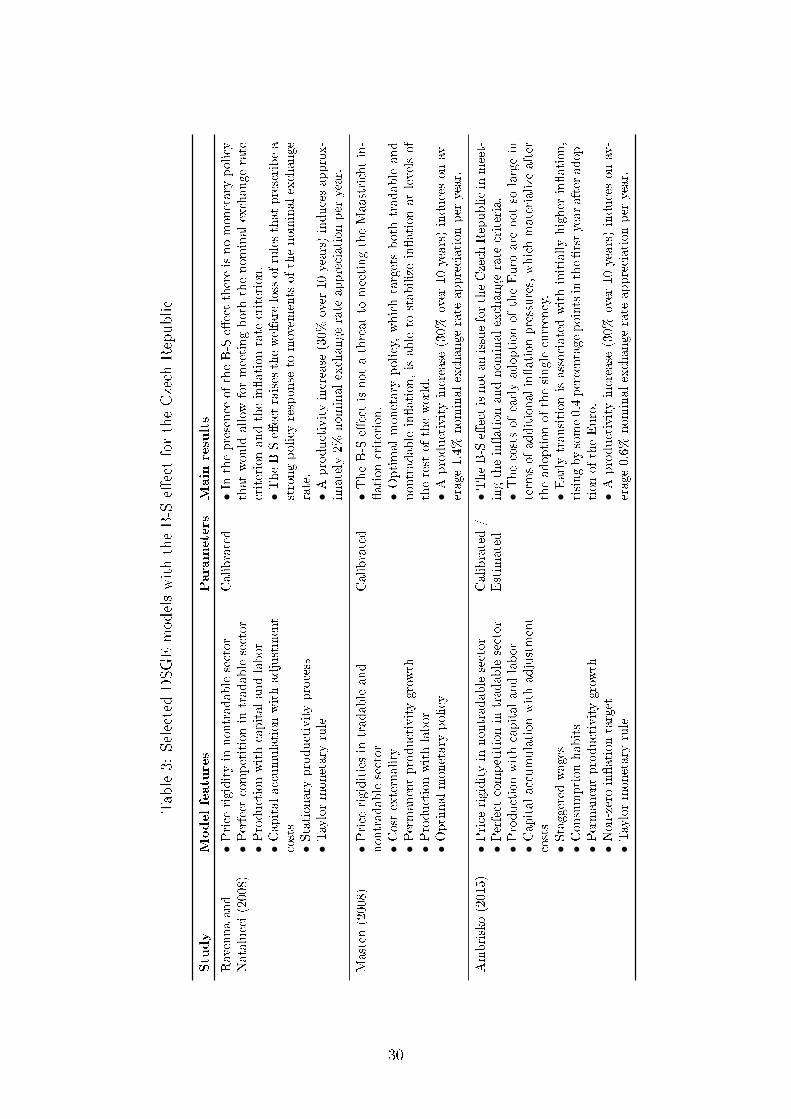
Table3:

Selected

DSG

EmodelswiththeB-S

e�ectfortheCzech

Repub

lic

Study

Modelfeatures

Parameters

Main

results

Ravenna

and

Natalucci(2008)

•Price

rigidity

innontradablesector

•Perfect

competitionin

tradablesector

•Produ

ctionwithcapitalandlabor

•Capital

accumulationwithadjustment

costs

•Stationary

productivity

process

•Taylormonetaryrule

Calibrated

•In

thepresence

oftheB-S

e�ectthereisno

monetarypolicy

that

would

allowformeeting

boththenominal

exchange

rate

criterionandthein�ation

rate

criterion.

•The

B-S

e�ectraises

thewelfare

lossofrulesthat

prescribea

strong

policyresponse

tomovem

entsof

thenominalexchange

rate.

•Aproductivity

increase

(30%

over

10years)indu

cesapprox-

imately2%

nominal

exchange

rate

appreciation

per

year.

Masten(2008)

•Price

rigidities

intradableand

nontradablesector

•Costexternality

•Permanentproductivity

grow

th•Produ

ctionwithlabor

•Optim

almonetarypolicy

Calibrated

•The

B-S

e�ectisnotathreat

tomeeting

theMaastrichtin-

�ation

criterion.

•Optim

almonetarypolicy,

which

targetsbothtradable

and

nontradablein�ation,isableto

stabilize

in�ation

atlevelsof

therest

oftheworld.

•A

productivity

increase

(30%

over

10years)

indu

ceson

av-

erage1.4%

nominal

exchange

rate

appreciation

per

year.

Ambrisko

(2015)

•Price

rigidity

innontradablesector

•Perfect

competitionin

tradablesector

•Produ

ctionwithcapitalandlabor

•Capital

accumulationwithadjustment

costs

•Staggeredwages

•Consumptionhabits

•Permanentproductivity

grow

th•Non-zeroin�ation

target

•Taylormonetaryrule

Calibrated/

Estim

ated

•The

B-S

e�ectisnotan

issuefortheCzech

Repub

licinmeet-

ingthein�ation

andnominal

exchange

rate

criteria.

•The

costsof

earlyadoption

oftheEuroarenotso

largein

term

sof

additionalin�ation

pressures,which

materializeafter

theadoption

ofthesinglecurrency.

•Early

transition

isassociated

withinitially

higher

in�ation,

rising

bysome0.4percentagepointsinthe�rstyear

afteradop-

tion

oftheEuro.

•A

productivity

increase

(30%

over

10years)

indu

ceson

av-

erage0.6%

nominal

exchange

rate

appreciation

per

year.

30

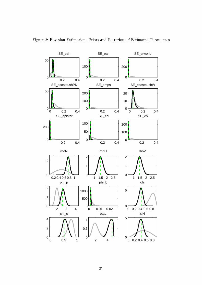
Figure 2: Bayesian Estimation: Priors and Posteriors of Estimated Parameters

0.2 0.40

50

SE_eah

0.2 0.40

100

SE_ean

0.2 0.40

200

SE_erworld

0 0.2 0.40

50

SE_ecostpushPN

0.2 0.40

100

200

SE_emps

0 0.2 0.40

10

20

SE_ecostpushW

0.2 0.40

200

SE_epistar

0.2 0.40

50

100

SE_ed

0.2 0.40

100

200

SE_es

0.2 0.4 0.6 0.8 10

5

rhoN

1 1.5 2 2.50

1

2

rhoH

1 1.5 2 2.50

1

2

rhoV

2 3 40

1

2

phi_p

0 0.01 0.020

500

1000

phi_b

0 0.2 0.4 0.6 0.80

5

chi

0 0.5 10

2

4

chi_c

2 40

0.5

1

etaL

0 0.2 0.4 0.6 0.80

5xiN

31

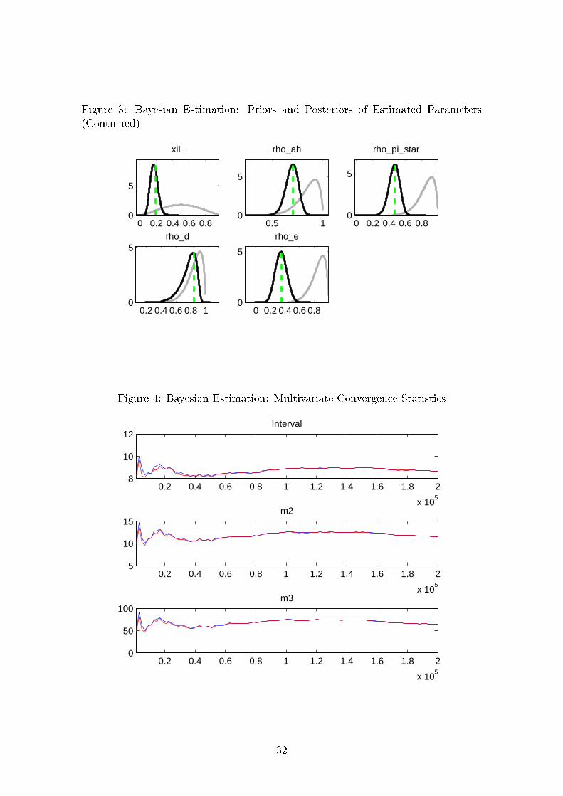
Figure 3: Bayesian Estimation: Priors and Posteriors of Estimated Parameters(Continued)

0 0.2 0.4 0.6 0.80

5

xiL

0.5 10

5

rho_ah

0 0.2 0.4 0.6 0.80

5

rho_pi_star

0.2 0.4 0.6 0.8 10

5rho_d

0 0.2 0.4 0.6 0.80

5

rho_e

Figure 4: Bayesian Estimation: Multivariate Convergence Statistics

0.2 0.4 0.6 0.8 1 1.2 1.4 1.6 1.8 2

x 105

8

10

12Interval

0.2 0.4 0.6 0.8 1 1.2 1.4 1.6 1.8 2

x 105

5

10

15m2

0.2 0.4 0.6 0.8 1 1.2 1.4 1.6 1.8 2

x 105

0

50

100m3

32

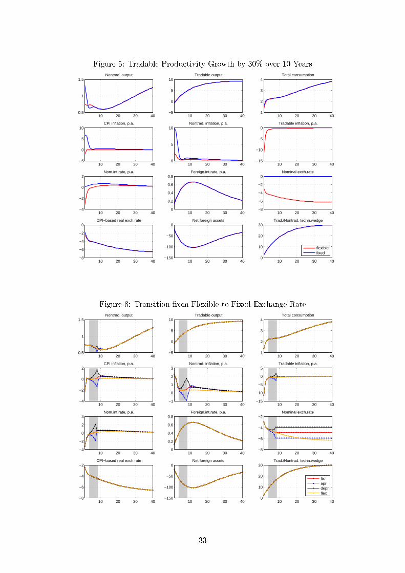
Figure 5: Tradable Productivity Growth by 30% over 10 Years

10 20 30 400.5

1

1.5Nontrad. output

10 20 30 40−5

0

5

10Tradable output

10 20 30 401

2

3

4Total consumption

10 20 30 40−5

0

5

10CPI inflation, p.a.

10 20 30 400

5

10Nontrad. inflation, p.a.

10 20 30 40−15

−10

−5

0Tradable inflation, p.a.

10 20 30 40−4

−2

0

2Nom.int.rate, p.a.

10 20 30 400

0.2

0.4

0.6

0.8Foreign.int.rate, p.a.

10 20 30 40−8

−6

−4

−2

0Nominal exch.rate

10 20 30 40−8

−6

−4

−2

0CPI−based real exch.rate

10 20 30 40−150

−100

−50

0Net foreign assets

10 20 30 400

10

20

30Trad./Nontrad. techn.wedge

flexiblefixed

balsam model Impulse response functions − compared 21−Jul−2015 18:40:31

Figure 6: Transition from Flexible to Fixed Exchange RateNontrad. output

10 20 30 400.5

1

1.5Tradable output

10 20 30 40−5

0

5

10Total consumption

10 20 30 401

2

3

4

CPI inflation, p.a.

10 20 30 40−4

−2

0

2Nontrad. inflation, p.a.

10 20 30 40−1

0

1

2

3Tradable inflation, p.a.

10 20 30 40−15

−10

−5

0

5

Nom.int.rate, p.a.

10 20 30 40−4

−2

0

2

4Foreign.int.rate, p.a.

10 20 30 400

0.2

0.4

0.6

0.8Nominal exch.rate

10 20 30 40−8

−6

−4

−2

CPI−based real exch.rate

10 20 30 40−8

−6

−4

−2Net foreign assets

10 20 30 40−150

−100

−50

0Trad./Nontrad. techn.wedge

10 20 30 400

10

20

30

fixaprdeprflex

balsam model B−S shock: transition from flexible to fixed 22−Jul−2015 17:52:28

33

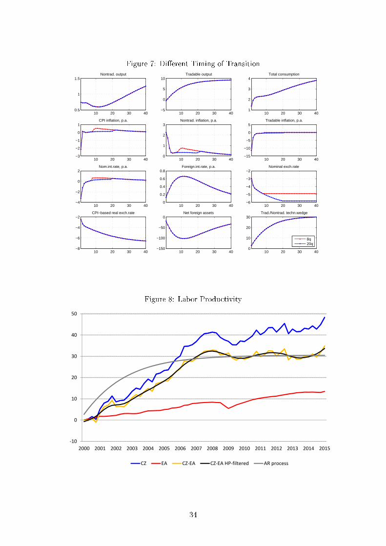
Figure 7: Di�erent Timing of Transition

10 20 30 400.5

1

1.5Nontrad. output

10 20 30 40−5

0

5

10Tradable output

10 20 30 401

2

3

4Total consumption

10 20 30 40−3

−2

−1

0

1CPI inflation, p.a.

10 20 30 400

1

2

3Nontrad. inflation, p.a.

10 20 30 40−15

−10

−5

0

5Tradable inflation, p.a.

10 20 30 40−4

−2

0

2Nom.int.rate, p.a.

10 20 30 400

0.2

0.4

0.6

0.8Foreign.int.rate, p.a.

10 20 30 40−6

−5

−4

−3

−2Nominal exch.rate

10 20 30 40−8

−6

−4

−2CPI−based real exch.rate

10 20 30 40−150

−100

−50

0Net foreign assets

10 20 30 400

10

20

30Trad./Nontrad. techn.wedge

8q20q

balsam model B−S shock: transition from flexible to fixed 21−Jul−2015 19:46:19

Figure 8: Labor Productivity

-10

0

10

20

30

40

50

2000 2001 2002 2003 2004 2005 2006 2007 2008 2009 2010 2011 2012 2013 2014 2015

CZ EA CZ-EA CZ-EA HP-filtered AR process

34

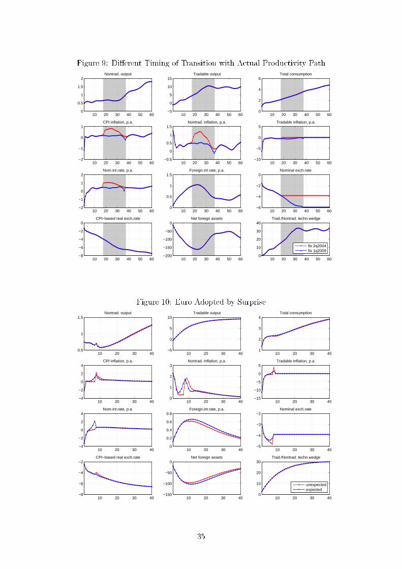
Figure 9: Di�erent Timing of Transition with Actual Productivity PathNontrad. output

10 20 30 40 50 600

0.5

1

1.5

2Tradable output

10 20 30 40 50 60−5

0

5

10

15Total consumption

10 20 30 40 50 600

2

4

6

CPI inflation, p.a.

10 20 30 40 50 60−2

−1

0

1Nontrad. inflation, p.a.

10 20 30 40 50 60−0.5

0

0.5

1

1.5Tradable inflation, p.a.

10 20 30 40 50 60−10

−5

0

5

Nom.int.rate, p.a.

10 20 30 40 50 60−2

−1

0

1

2Foreign.int.rate, p.a.

10 20 30 40 50 600

0.5

1

1.5Nominal exch.rate

10 20 30 40 50 60−6

−4

−2

0

CPI−based real exch.rate

10 20 30 40 50 60−8

−6

−4

−2

0Net foreign assets

10 20 30 40 50 60−200

−150

−100

−50

0Trad./Nontrad. techn.wedge

10 20 30 40 50 600

10

20

30

40

fix 2q2004fix 1q2009

balsam model B−S shock: transition from flexible to fixed 21−Jul−2015 19:42:15

Figure 10: Euro Adopted by Surprise

10 20 30 400.5

1

1.5Nontrad. output

10 20 30 40−5

0

5

10Tradable output

10 20 30 401

2

3

4Total consumption

10 20 30 40−4

−2

0

2

4CPI inflation, p.a.

10 20 30 400

1

2

3Nontrad. inflation, p.a.

10 20 30 40−15

−10

−5

0

5Tradable inflation, p.a.

10 20 30 40−4

−2

0

2

4Nom.int.rate, p.a.

10 20 30 400

0.2

0.4

0.6

0.8Foreign.int.rate, p.a.

10 20 30 40−5

−4

−3

−2Nominal exch.rate

10 20 30 40−8

−6

−4

−2CPI−based real exch.rate

10 20 30 40−150

−100

−50

0Net foreign assets

10 20 30 400

10

20

30Trad./Nontrad. techn.wedge

unexpectedexpected

balsam model B−S shock: transition from flexible to fixed 21−Jul−2015 19:46:23

35

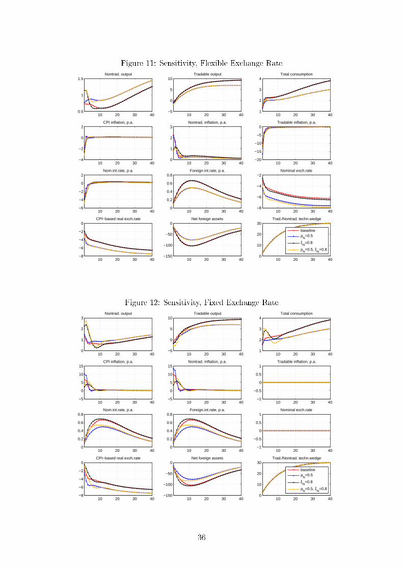
Figure 11: Sensitivity, Flexible Exchange Rate

10 20 30 400.5

1

1.5Nontrad. output

10 20 30 40−5

0

5

10Tradable output

10 20 30 401

2

3

4Total consumption

10 20 30 40−4

−2

0

2CPI inflation, p.a.

10 20 30 400

1

2

3Nontrad. inflation, p.a.

10 20 30 40−20

−15

−10

−5

0Tradable inflation, p.a.

10 20 30 40−6

−4

−2

0

2Nom.int.rate, p.a.

10 20 30 400

0.2

0.4

0.6

0.8Foreign.int.rate, p.a.

10 20 30 40−8

−6

−4

−2Nominal exch.rate

10 20 30 40−8

−6

−4

−2

0CPI−based real exch.rate

10 20 30 40−150

−100

−50

0Net foreign assets

10 20 30 400

10

20

30Trad./Nontrad. techn.wedge

baselineρ

N=0.5

ξN

=0.8

ρN

=0.5, ξN

=0.8

balsam model B−S shock: flexible exchange rate 22−Jul−2015 17:59:24

Figure 12: Sensitivity, Fixed Exchange Rate

10 20 30 400

1

2

3Nontrad. output

10 20 30 40−5

0

5

10Tradable output

10 20 30 401

2

3

4Total consumption

10 20 30 40−5

0

5

10

15CPI inflation, p.a.

10 20 30 40−5

0

5

10

15Nontrad. inflation, p.a.

10 20 30 40−1

−0.5

0

0.5

1Tradable inflation, p.a.

10 20 30 400

0.2

0.4

0.6

0.8Nom.int.rate, p.a.

10 20 30 400

0.2

0.4

0.6

0.8Foreign.int.rate, p.a.

10 20 30 40−1

−0.5

0

0.5

1Nominal exch.rate

10 20 30 40−8

−6

−4

−2

0CPI−based real exch.rate

10 20 30 40−150

−100

−50

0Net foreign assets

10 20 30 400

10

20

30Trad./Nontrad. techn.wedge

baselineρ

N=0.5

ξN

=0.8

ρN

=0.5, ξN

=0.8

balsam model B−S shock: fixed exchange rate 22−Jul−2015 17:59:30

36

Working Paper Series ISSN 1211-3298 Registration No. (Ministry of Culture): E 19443 Individual researchers, as well as the on-line and printed versions of the CERGE-EI Working Papers (including their dissemination) were supported from institutional support RVO 67985998 from Economics Institute of the ASCR, v. v. i. Specific research support and/or other grants the researchers/publications benefited from are acknowledged at the beginning of the Paper. (c) Róbert Ambriško, 2015 All rights reserved. No part of this publication may be reproduced, stored in a retrieval system or transmitted in any form or by any means, electronic, mechanical or photocopying, recording, or otherwise without the prior permission of the publisher. Published by Charles University in Prague, Center for Economic Research and Graduate Education (CERGE) and Economics Institute of the ASCR, v. v. i. (EI) CERGE-EI, Politických vězňů 7, 111 21 Prague 1, tel.: +420 224 005 153, Czech Republic. Printed by CERGE-EI, Prague Subscription: CERGE-EI homepage: http://www.cerge-ei.cz Phone: + 420 224 005 153 Email: office@cerge-ei.cz Web: http://www.cerge-ei.cz Editor: Marek Kapička The paper is available online at http://www.cerge-ei.cz/publications/working_papers/. ISBN 978-80-7343-353-6 (Univerzita Karlova v Praze, Centrum pro ekonomický výzkum a doktorské studium) ISBN 978-80-7344-345-0 (Národohospodářský ústav AV ČR, v. v. i.)