Numerical Modeling in Geotechnical Engineering 1 October ... · 3 Main References FLAC, Fast Lagrangian Analysis of Continua Manual, Itasca Inc., 2013 Steven F. Bartlett, Numerical

PRESENTED BY: Siavash Zamiran

Ph.D. Student, Research and Teaching Assistant, Department of

Civil Engineering, Southern Illinois University Carbondale

Email: [email protected]

Website: www.zamiran.net

Linkedin: www.linkedin.com/in/zamiran

Numerical Modeling in Geotechnical Engineering 1

October 17, 18 2014

Workshop Schedule 2

Date Time Session Room

October 17 , 2014 9 AM to 10:30 AM Session 1 EB 0160

October 17 , 2014 10:45 AM to 12:15 PM Session 2 EB 0160

October 17 , 2014 2 PM to 3:30 PM Session 3 EB 1140

October 17 , 2014 3:45 PM to 5:15 PM Session 4 EB 1140

October 18 , 2014 9 AM to 10:30 AM Session 5 EB 1140

October 18 , 2014 10:45 AM to 12:15 PM Session 6 EB 1140

October 18 , 2014 2 PM to 3:30 PM Session 7 EB 1140

October 18 , 2014 3:45 PM to 5:15 PM Session 8 EB 1140

Main References 3

FLAC, Fast Lagrangian Analysis of Continua Manual, Itasca Inc., 2013

Steven F. Bartlett, Numerical Methods in Geotechnical Engineering,

The University of Utah, 2012

Soil Mechanics

Foundation Engineering

Strength of Material

Prerequisites 4

Outline 5

•Introduction to Numerical Modeling in Geotechnical

Engineers

• Numerical Modeling Using FLAC

•Foundation, Stone Column Modeling

•Slope Stability Analysis

•Structural Elements

•Seismic Considerations

Introduction to Numerical Modeling in

Geotechnical Engineers

Chapter 1 6

Numerical modeling approach 7

Simple definition of modeling 8

Application of modeling 9

Numerical modeling procedure 10

Numerical Techniques 11

Numerical Techniques

•Finite Element

•Finite Difference

Commercially Available Software Packages

○ FLAC (Fast Lagrangian Analysis of Continua) (General FDM)

○ ABAQUS (FEM) (General FEM with some geotechnical relations)

○ ANSYS (FEM) (Mechanical/Structural)

○ PLAXIS (FEM) (Geotechnical)

○ SIGMA/W (FEM) (Geotechnical)

○ SEEP/W (FEM) (Seepage Analysis)

○ MODFLOW (FEM) (Groundwater Modeling)

FLAC and PLAXIS are the most commonly used by advanced

geotechnical consultants

Numerical Modeling Procedure 12

Selection of representative cross-section

• Idealize the field conditions into a design X-section

• Plane strain vs. axisymmetrical models

Choice of numerical scheme and constitutive relationship

• FEM vs FDM

• Elastic vs Mohr-Coulomb vs. Elastoplastic models

Characterization of material properties for use in model

• Strength

• Stiffness

• Stress - Strain Relationships

Grid generation

• Discretize the Design X-section into nodes or elements

Assign of materials properties to grid

Assigning boundary conditions

Calculate initial conditions

Determine loading or modeling sequence

Run the model

Obtain results

Interpret of results

Idealize Field Conditions to Numerical Modeling

13

• Complex site situation should be simplified reasonably for modeling

• Many 3D problems can be reduced to 2D problems by selection of

the appropriate X-sections.

Note for plane strain conditions to exist all strains are in the x-y coordinate system

(i.e., x-y plane). There is no strain in the z direction (i.e., out of the paper

direction). This usually implies that the structure or feature is relatively long, so

that the z direction and the balanced stresses in this direction have little influence

on the behavior within the selected cross section.

Plain Strain Numerical Modeling Examples

14

Deformation analysis of slopes Deformation analysis of tunnels


15

Dynamic analysis MSE walls


16

Retaining wall Embankment dam


17

Strip footing Roadway embankment

Axisymmetrical Conditions 18

Axisymmetrical Numerical Modeling Examples

19

Circular Footing Single Pile

20

Flow to an injection and/or pumping well

Point Load on Soil

Axisymmetrical Numerical Modeling Examples

Finite Element vs Finite Difference 21

Finite Element Method 22

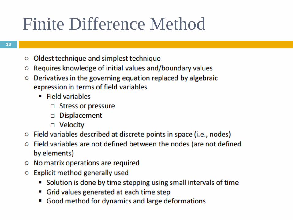
Finite Difference Method 23

Basic explicit calculation cycle 24

Constitutive Relationships 25

Constitutive Models: (i.e., stress-strain laws)

• Elastic: can be described by the linear elasticityequations such as

Hooke's law

•Viscoelastic: These are materials that behave elastically, but also

have damping: when the stress is applied and removed, work has to

be done against the damping effects. This implies that the material

response has time-dependence.

•Elaso-plastic: Materials that behave elastically generally do so

when the applied stress is less than a yield value. When the stress is

greater than the yield stress, the material behaves plastically and

does not return to its previous state. That is, deformation that occurs

after yield is permanent.

Constitutive Relationships II 26

Numerical Modeling Using FLAC

Chapter 2 27

Itasca Consulting Group, Inc. 28

•Itasca is a global, employee-owned, engineering consulting and

software firm

•Are of concentration: mining, civil engineering, oil & gas,

manufacturing and power generation

•Since 1981

• Provides:

FLAC

FLAC3D

Flac/ Slope

PFC

Kubrix

3DEC

UDEC

Download a demo version 29

szamira -as

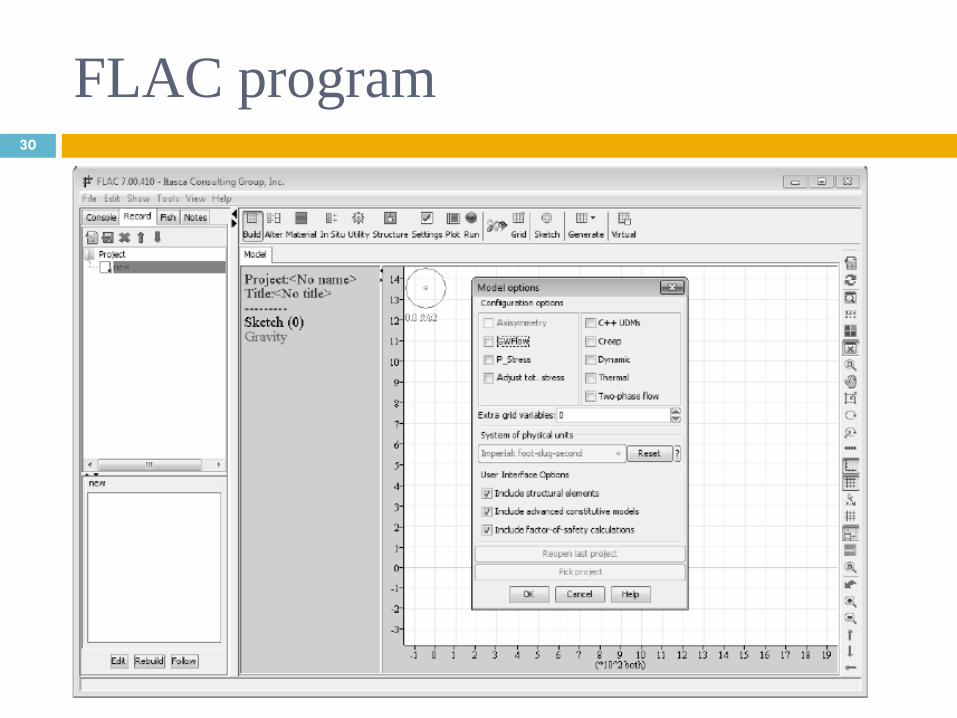
FLAC program 30

31

32

Terminology 33

Special Features 34

Field Equations in FLAC 35

Solution of solid-body: equations of motion and constitutive relations

Heat-transfer: Fourier’s Law for conductive heat transfer

Fluid-flow problems: Darcy’s Law

Motion and Equilibrium

Normal and Shear Stresses 36

Normal and Shear Strain 37

Strain - Displacement 38

Hooke’s law 39

Bulk Modulus 40

where P is pressure, Vis volume, and ∂P/∂Vdenotes the partial derivative of

pressure with respect to volume.

Elastic Correlations 41

Motion and Equilibrium 42

In a continuous solid body:

Constitutive Relation 43

strain rate is derived from velocity gradient as follows

Constitutive Model 44

The simplest example of a constitutive law is that of isotropic

elasticity:

Finite Difference Zones 45

Zone and Gridpoint 46

Finite Difference Grid with 400 zones 47

Zone Numbers 48

Grid Point Numbers 49

Boundary Condition 50

Initital Conditions 51

Boundary Conditions 52

Applied Condition 53

Modeling Steps 54

•Generate a grid for the domain

•Assign Constitutive Model

•Assign material properties

•Assign boundary/loading conditions

•Solve for the system of algebraic equations using the initial

conditions and the boundary conditions (This usually done

by time stepping in an explicit formulation.)

•Implement the solution in computer code to perform the

calculations.

Numerical Flowchart 55

Grids 56

General solution procedure:

Start: COMMAND keyword value . . . <keyword value . . . > . . .

; comments

grid icol jrow

grid 10 10

model elastic

grid 20,20

model elas

gen 0,5 0,20 20,20 5,5 i=1,11

gen same same 20,0 5,0 i=11,21

grid 20,20

m e

gen 0,0 0,100 100,100 100,0 rat 1.25 1.25

57

gr 10,10

m e

gen -100,0 -100,100 0,100 0,0 rat .80,1.25

Creating a circular hole in a grid

new

grid 20,20

m e

gen circle 10,10 5

model null region 10,10


Moving gridpoints with the INITIAL command

new

grid 5 5

model elastic

gen 0,0 0,10 10,10 10,0

ini x=-2 i=1 j=6

ini x=12 i=6

58

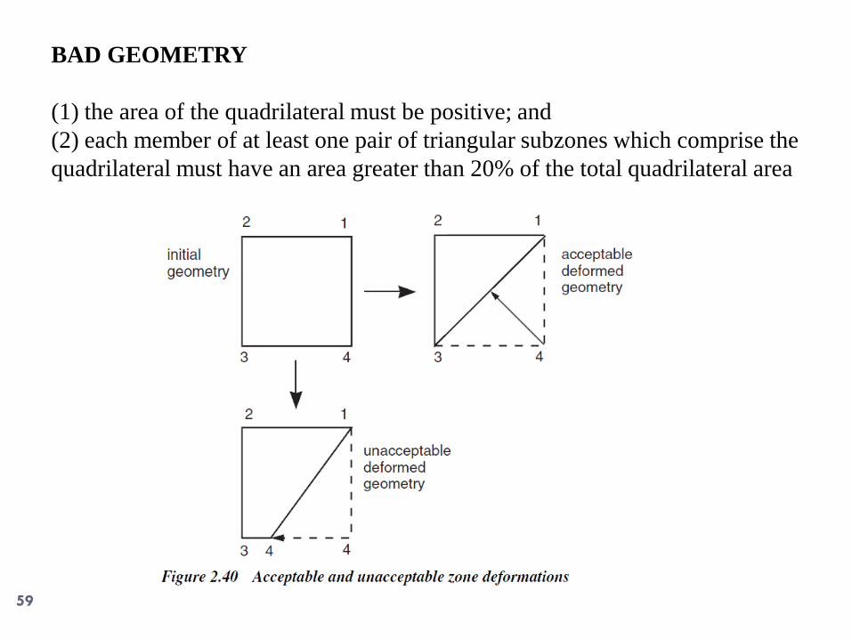
BAD GEOMETRY

(1) the area of the quadrilateral must be positive; and

(2) each member of at least one pair of triangular subzones which comprise the

quadrilateral must have an area greater than 20% of the total quadrilateral area

59

Assigning Material Models

Elastic Model MODEL elastic and MODEL mohr-coul require that material properties be

assigned via the PROPERTY

command. For the elastic model, the required properties are

(1) density;

(2) bulk modulus; and

(3) shear modulus.

60

Mohr-Coulomb plasticity model (1) density;

(2) bulk modulus;

(3) shear modulus;

(4) friction angle;

(5) cohesion;

(6) dilation angle; and

(7) tensile strength.

grid 10,10

model elas j=6,10

prop den=2000 bulk=1e8 shear=.3e8 j=6,10

model mohr j=1,5

prop den=2500 bulk=1.5e8 shear=.6e8 j=1,5

prop fric=30 coh=5e6 ten=8.66e6 j=1,5

61

Applying Boundary and Initial Conditions

62

Sign Conventions

DIRECT STRESS – Positive stresses indicate tension; negative stresses indicate

compression.

SHEAR STRESS

63

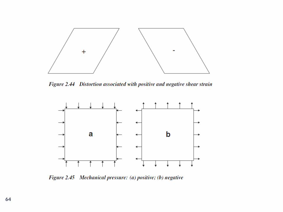
64

PORE PRESSURE – Fluid pore pressure is positive in compression. Negative

pore pressure

indicates fluid tension.

GRAVITY – Positive gravity will pull the mass of a body downward (in the

negative y-direction).

Negative gravity will pull the mass of a body upward.

65

66

67

;Example

grid 10 10

mod el

fix x i=1

fix x i=11

fix y j=1

app press = 10 j=11

ini sxx=-10 syy=-10

hist unbal

hist xvel i=5 j=5

hist ydisp i=5 j=11

68

grid 10 10

mod el

prop d=1800 bulk=1e8 shear =.3e8

fix x i=1

fix x i=11

fix y j=1

app pres=1e6 j=11

hist unbal

hist ydisp i=5 j=11

ini sxx=-1e6 syy=-1e6 szz=-1e6

set gravity=9.81

step 900

69

Performing Alterations

FLAC allows model conditions to be changed at any point in the solution

process. These changes

may be of the following forms.

• excavation of material

• addition or deletion of gridpoint loads or pressures

• change of material model or properties for any zone

• fix or free velocities for any gridpoint

;Example

grid 10,10

model elastic

gen circle 5,5 2

plot hold grid

gen adjust

plot hold grid

prop s=.3e8 b=1e8 d=1600

set grav=9.81

fix x i=1

fix x i=11

fix y j=1

solve

ini sxx 0.0 syy 0.0 szz 0.0 region 5,5

prop s .3e5 b 1e5 d 1.6 region 5,5

;mod null region 5,5

solve

70

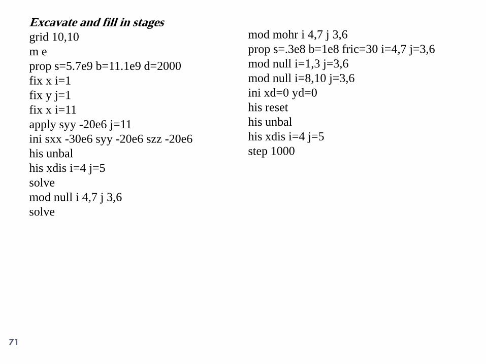
Excavate and fill in stages

grid 10,10

m e

prop s=5.7e9 b=11.1e9 d=2000

fix x i=1

fix y j=1

fix x i=11

apply syy -20e6 j=11

ini sxx -30e6 syy -20e6 szz -20e6

his unbal

his xdis i=4 j=5

solve

mod null i 4,7 j 3,6

solve

mod mohr i 4,7 j 3,6

prop s=.3e8 b=1e8 fric=30 i=4,7 j=3,6

mod null i=1,3 j=3,6

mod null i=8,10 j=3,6

ini xd=0 yd=0

his reset

his unbal

his xdis i=4 j=5

step 1000

71

Saving/Restoring Problem State

save file.sav

rest file.sav

save fill1.sav

72

Foundation, Stone Column Modeling

Chapter 3 73

Foundation and stone column modeling

74

Example 1:

;------------STAGE 1-----------------

config

grid 80 40

model elastic i=1,80 j=1,20

gen 0,0 0,5 20,5 20,0 i=1,81 j=1,21

prop b=8.3e6 s= 3.8e6 d=1800 i=1,80

j=1,20

fix x i=1

fix x i=81

fix x y j=1

set g=9.81

history unbal

;solve

ini xdisp=0 ydisp=0

;


75

;------------STAGE 2-----------------

model mohr i=1,80 j=1,20

apply press=100e3 i=38,45 j=21

prop b=8.3e6 s= 3.8e6 d=1800 c=30e3

f=10 i=1,80 j=1,20

set large

;solve

76

;Example 2:

;------------STAGE 1-----------------

config

grid 80 40


gen 0,0 0,5 20,5 20,0 i=1,81 j=1,21

fix x i=1

fix x i=81

fix x y j=1

set g=9.81

history unbal

group layer1 j=1,8

group layer2 j=9,16

group layer3 j=17,20

prop b=1.6e7 s= 7.6e6 d=1800 group layer1



solve


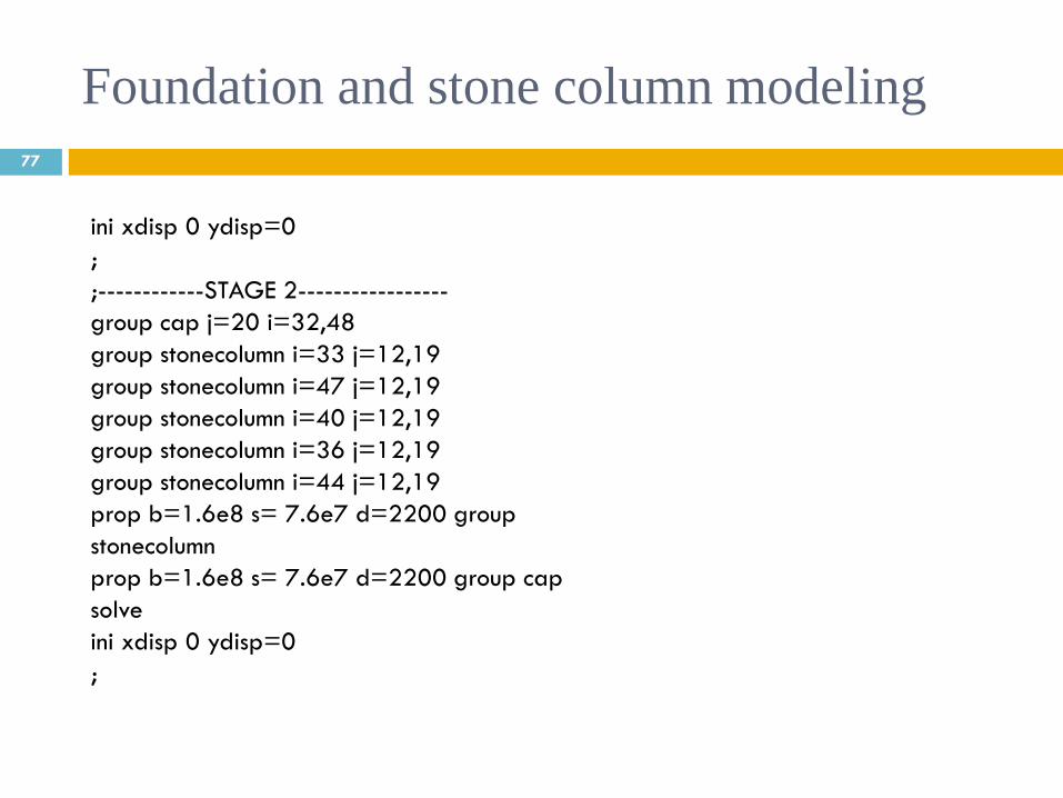
77

ini xdisp 0 ydisp=0

;

;------------STAGE 2-----------------

group cap j=20 i=32,48

group stonecolumn i=33 j=12,19





prop b=1.6e8 s= 7.6e7 d=2200 group

stonecolumn

prop b=1.6e8 s= 7.6e7 d=2200 group cap

solve

ini xdisp 0 ydisp=0

;


78

;------------STAGE 3-----------------

model mohr group layer1



prop b=1.6e7 s= 7.6e6 d=1800 c=35e3

f=10 group layer1

prop b=1.5e6 s= 6.9e5 d=2000 f=25 group

layer2

prop b=1.6e7 s= 7.6e6 d=2000 c=35e3

f=12 group layer3


solve


79


80

Example 3:

;------------STAGE 1-----------------

config

grid 80 40


gen 0,0 0,5 20,5 20,0 i=1,81 j=1,21

fix x i=1

fix x i=81

fix x y j=1

set g=9.81

history unbal

group layer1 j=1,8

group layer2 j=9,16

group layer3 j=17,20




solve


81

ini xdisp 0 ydisp=0

;

;------------STAGE 2-----------------

group cap j=20 i=32,48

prop b=1.6e8 s= 7.6e7 d=2200 group cap

solve

ini xdisp 0 ydisp=0

;------------STAGE 3-----------------




prop b=1.6e7 s= 7.6e6 d=1800 c=35e3

f=10 group layer1

prop b=1.5e6 s= 6.9e5 d=2000 f=25 group

layer2

prop b=1.6e7 s= 7.6e6 d=2000 c=35e3

f=12 group layer3


solve


82


83

0

1

2

3

4

5

6

-10 -8 -6 -4 -2 0

He

igh

t (m

)

Settlement (cm)

Settlement (cm)

Settlement (With Stone Column) (cm)


Slope Stability Analysis

Chapter 4 84

Groundwater simulation 85

•Water table

•Steady state analysis

•Transient analysis

Slope stability analysis – Dry 86

config ats

grid 20,10

m m

prop s=.3e8 b=1e8 d=1500 fri=20 coh=1e10

ten=1e10

; warp grid to form a slope :

gen 0,0 0,3 20,3 20,0 j 1,4

gen same 9,10 20,10 same i 6 21 j 4 11

mark i=1,6 j=4

mark i=6 j=4,11


; displacement boundary conditions

fix x i=1

fix x i=21

fix x y j=1

; apply gravity

set grav=9.81

; soil properties -- note large

cohesion to force initial elastic

; behavior for determining

initial stress state. This will

prevent ; slope failure when

initializing the gravity stresses

Slope stability analysis – Dry 87

; displacement history of slope

his ydis i=10 j=10

; solve for initial gravity stresses

solve

;

;*** BRANCH: DRY ****

;... STATE: SL2 ....

; reset displacement components to zero

ini xdis=0 ydis=0

; set cohesion to 0

prop coh=0

; use large strain logic

set large

step 200

;save sl2.sav

step 800

solve

; Change cohesion to c=10e3

; soil properties -- note large

cohesion to force initial elastic

; behavior for determining

initial stress state. This will

prevent ; slope failure when

initializing the gravity stresses

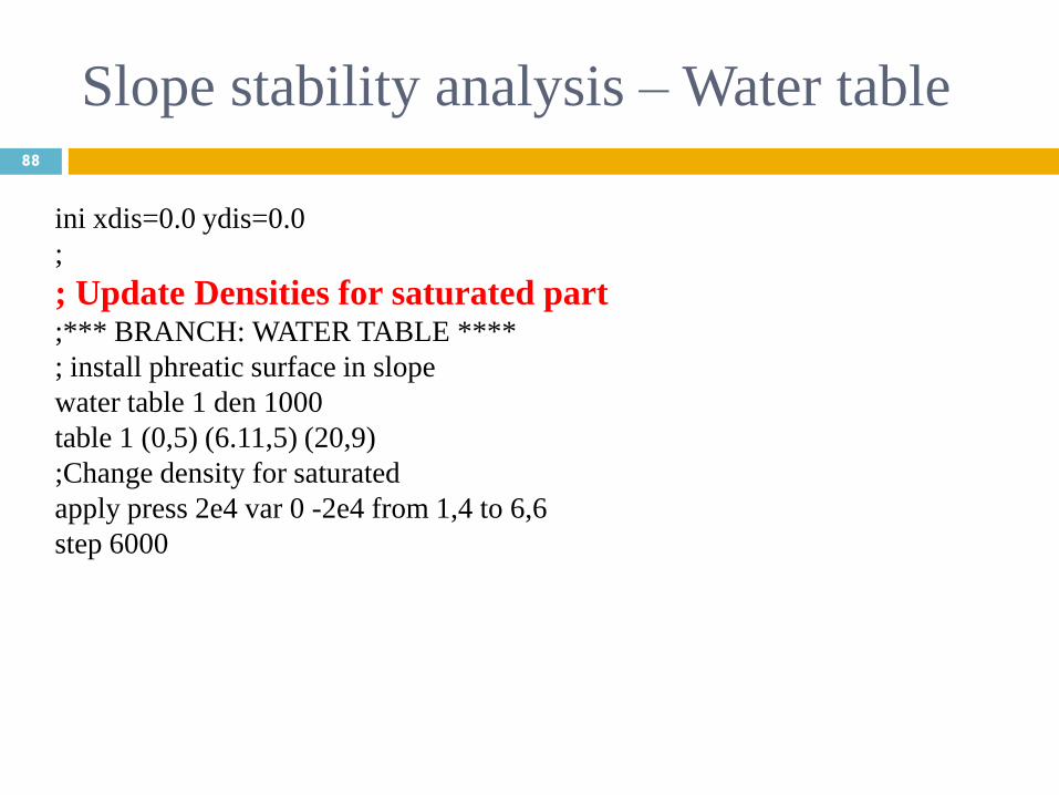
Slope stability analysis – Water table 88

ini xdis=0.0 ydis=0.0

;

; Update Densities for saturated part ;*** BRANCH: WATER TABLE ****

; install phreatic surface in slope

water table 1 den 1000

table 1 (0,5) (6.11,5) (20,9)

;Change density for saturated

apply press 2e4 var 0 -2e4 from 1,4 to 6,6

step 6000

Permeability 89

Slope stability analysis – Groundwater 90

config gw ats

grid 20,10

; Type "new" to start a new problem

;Mohr-Coulomb model

m m

prop s=.3e8 b=1e8 d=1500 fri=20 coh=1e10 ten=1e10

; warp grid to form a slope :

gen 0,0 0,3 20,3 20,0 j 1,4

gen same 9,10 20,10 same i 6 21 j 4 11

mark i=1,6 j=4

mark i=6 j=4,11


prop perm 1e-10 por .3

water den 1000 bulk 1e4


; displacement boundary conditions

fix x i=1

fix x i=21

fix x y j=1

; pore pressure boundary conditions

apply pp 9e4 var 0 -9e4 i 21 j 1 10

apply pp 5e4 var 0 -3e4 i 1 j 1 4

ini pp 2e4 var 0 -2e4 mark i 1 6 j 4 6

fix pp mark

; apply gravity

set grav=9.81

hist gwtime

set mech off

solve


;... STATE: SLGW3 ....

set flow off mech on

app press 2e4 var 0 -2e4 from 1 4 to 6 6

water bulk 0.0

; displacement history of slope

hist reset

his ydis i=10 j=10

solve

;... STATE: SLGW4 ....

ini xdis 0.0 ydis 0.0

prop coh 1e4 ten 0.0

set large

solve

Structural elements

Chapter 5 93

Structural element 94

•Beam

•Pile

•Cable

Nail and Anchor modeling 95

t is annulus thickness of the shear zone and is

considered equal to 0.004 m.

Material properties 96

Codes 97

struct node 1501 0.0 0.0

struct node 1500 0.0 -32.0

struct beam beg node 1500 end node 1501 prop 1001 seg 32

struct prop 1001

int 101 as from 31,35 to 31,67 bs from node 1500 to node 1501

int 102 as from 32,67 to 32,35 bs from node 1501 to node 1500

struct prop 1001 density 2400.0

struct cable begin node 1533 end node 1534 seg 1 tension 768000.0 prop 2001

struct cable begin node 1535 end node 1533 seg 6 prop 2002

struct prop 2002

struct prop 2001 spac 2.3 e 2.1E11 area 0.0015 yie 1e10 kb 0 sb 0

struct prop 2002 spac 2.3 e 2.1E11 area 0.0015 yie 1e10 kb 1.0E8 sb 1e8

Seismic Considerations

Chapter 6 98

Important points 99

•Loading

•Damping

•Boundary condition

Boundary conditions 100

Boundary conditions 101

Codes 102

config dyn

set dyn off

set dyn on

apply xquiet j=1

apply ff

apply nquiet squiet j=1 ;(bottom)

;----------------------damping

set dy_damp struc rayl 0.05 1.64 mass

set dy_damp rayl 0.05 1.64

apply sxy 4.8e5 hist table 1 j 1

set dytime 0

hist reset

hist dytime

his 10 xacc i=50 j=2

his 11 xacc i=50 j=26

solve dytime 4

table 1 0 0

table 1 0.02 -0.146

table 1 0.04 -0.374

table 1 0.06 -0.574

table 1 0.08 -0.761

table 1 0.1 -0.973

table 1 0.12 -1.223

table 1 0.14 -1.473

table 1 0.16 -1.682

table 1 0.18 -1.842

table 1 0.2 -1.97

table 1 0.22 -2.138

table 1 0.24 -2.389

table 1 0.26 -2.693

table 1 0.28 -2.971

table 1 0.3 -3.189

table 1 0.32 -3.345

table 1 0.34 -3.434

Documents

Numerical Modeling in Geotechnical Engineering 1 October ... · 3 Main References FLAC, Fast Lagrangian Analysis of Continua Manual, Itasca Inc., 2013 Steven F. Bartlett, Numerical