Nonlinear Finite Element Modeling of Cellular Materials

University of Rhode Island University of Rhode Island

DigitalCommons@URI DigitalCommons@URI

Open Access Master's Theses

2016

Nonlinear Finite Element Modeling of Cellular Materials Under Nonlinear Finite Element Modeling of Cellular Materials Under

Dynamic Loading and Comparison to Experiments Dynamic Loading and Comparison to Experiments

Colin J. Murphy University of Rhode Island, [email protected]

Follow this and additional works at: https://digitalcommons.uri.edu/theses

Recommended Citation Recommended Citation Murphy, Colin J., "Nonlinear Finite Element Modeling of Cellular Materials Under Dynamic Loading and Comparison to Experiments" (2016). Open Access Master's Theses. Paper 806. https://digitalcommons.uri.edu/theses/806

This Thesis is brought to you for free and open access by DigitalCommons@URI. It has been accepted for inclusion in Open Access Master's Theses by an authorized administrator of DigitalCommons@URI. For more information, please contact [email protected].

https://digitalcommons.uri.edu/

https://digitalcommons.uri.edu/theses

https://digitalcommons.uri.edu/theses?utm_source=digitalcommons.uri.edu%2Ftheses%2F806&utm_medium=PDF&utm_campaign=PDFCoverPages

https://digitalcommons.uri.edu/theses/806?utm_source=digitalcommons.uri.edu%2Ftheses%2F806&utm_medium=PDF&utm_campaign=PDFCoverPages

mailto:[email protected]

NONLINEAR FINITE ELEMENT MODELING OF CELLULAR MATERIALS

UNDER DYNAMIC LOADING AND COMPARISON TO EXPERIMENTS

BY

COLIN J. MURPHY

A THESIS SUBMITTED IN PARTIAL FULFILLMENT OF THE

REQUIREMENTS FOR THE DEGREE OF

MASTER OF SCIENCE

IN

MECHANICAL ENGINEERING AND APPLIED MECHANICS

UNIVERSITY OF RHODE ISLAND

2016

MASTER OF SCIENCE IN MECHANICAL ENGINEERING AND APPLIED

MECHANICS THESIS

OF

COLIN J. MURPHY

APPROVED:

Thesis Committee:

Major Professor Martin H. Sadd

Arun Shukla

George Tsiatas

Nasser H. Zawia

DEAN OF THE GRADUATE SCHOOL

UNIVERSITY OF RHODE ISLAND

2016

ABSTRACT

This study used an open source three-dimensional Voronoi cell software

library to create nonlinear finite element models of open cell metal foams in the 5% to

10% relative density range. Cubic and Body-Centered Cubic (BCC) seed point

generation techniques were compared. The impact of random positional perturbations

on original seed points was investigated as it relates to material stiffness and yield

strength. The models simulated a 10-cell cube of foam material under uniaxial loading

at strain rates of around 102/s up to about 80% compressive strain. It was shown that

the models created with BCC seed points generally had a higher modulus which was

less sensitive to perturbations in seed point location. The models were compared to

drop-weight experiments on ERG Duocel metal foams of 10, 20, and 40 Pores Per

Inch (PPI) which were filmed with a high speed camera. The models showed good

agreement with analytical predictions for material properties, but a comparison with

experimental data indicated that they lost accuracy in simulating material response

after 50% compressive strain. Past this point, cell-wall contact within the foam was a

dominant mechanism in the mechanical response, and model predictions did not

appear to match well with experimental data.

In a parallel experimental effort ERG foams of 10 PPI and around 8% relative

density were subjected to tensile loading at a strain rate of 73/s. High speed

photography was again used to interpret the data. The Young’s modulus and yield

strength of these foams were shown to increase by a factor of ten as compared to

quasistatic values, indicating significant rate dependence.

iii

ACKNOWLEDGMENTS

There are many people who have assisted with this effort and, more generally,

have offered advice and encouragement in my path as an engineer. First, thank you to

Dr. Martin Sadd who agreed to take on this project, agreed to advise a part time student,

and has been a dedicated and rigorous advisor. Dr. Arun Shukla provided invaluable

assistance by allowing access to his laboratory and equipment, and ideas and

suggestions for experiments. From his Dynamic Photomechanics Laboratory Dr. Nick

Heeder, Dr. Sachin Gupta, Prathmesh Parrikar, and Emad Makki provided assistance

with the experimental effort that was much appreciated. The Enhancement of Graduate

Research Awards Grant by URI’s Graduate School provided generous financial

assistance for the experimental portion of this study. At the Naval Undersea Warfare

Center: Dr. Fletcher Blackmon was instrumental in the decision to take on a thesis; Dr.

Jim Leblanc provided helpful discussion and an introduction to LS-DYNA; Scott

Weininger delivered excellent IT assistance in setting up a work station; and the Sensors

and SONAR Department provided financial support. At URI and NUWC Dr. Donna

Meyer and Dr. Jahn Torres have continually provided helpful conversations and much

needed mentorship. To my parents for their support and for an enriching childhood.

Finally, to my wife Ellen for her steadfast support for my dreams and her warm

friendship.

iv

TABLE OF CONTENTS

ABSTRACT .................................................................................................................. ii

ACKNOWLEDGMENTS .......................................................................................... iii

TABLE OF CONTENTS ............................................................................................ iv

LIST OF TABLES ...................................................................................................... vi

LIST OF FIGURES ................................................................................................... vii

CHAPTER 1 ................................................................................................................. 1

INTRODUCTION ...................................................................................................... 1

CHAPTER 2 ............................................................................................................... 12

REVIEW OF LITERATURE ................................................................................... 12

CHAPTER 3 ............................................................................................................... 27

FINITE ELEMENT MODELING ........................................................................... 27

3.1 PRELIMINARIES .......................................................................................... 27

3.2 SEED POINT GENERATION, PSEUDO-RANDOMIZATION, AND

VORONOI LATTICE COMPUTATION ............................................................ 28

3.3 FINITE ELEMENT MODEL INPUT PARAMETERS ................................. 33

3.4 FINITE ELEMENT MODEL RESULTS....................................................... 37

CHAPTER 4 ............................................................................................................... 46

COMPRESSION EXPERIMENTS .......................................................................... 46

4.1 INTRODUCTION .......................................................................................... 46

v

4.2 EXPERIMENTAL METHOD ........................................................................ 46

4.3 EXPERIMENT RESULTS AND DATA PROCESSING ............................. 49

CHAPTER 5 ............................................................................................................... 57

TENSION EXPERIMENTS .................................................................................... 57

5.1 INTRODUCTION .......................................................................................... 57

5.2 EXPERIMENTAL METHOD ........................................................................ 57

5.2 EXPERIMENT RESULTS AND DATA PROCESSING ............................. 60

CHAPTER 6 ............................................................................................................... 65

CONCLUSIONS ...................................................................................................... 65

6.1 COMPRESSION FEM AND EXPERIMENTS ............................................. 65

6.2 TENSION EXPERIMENTS ........................................................................... 68

6.3 CONCLUDING REMARKS AND RECOMMENDATIONS FOR

FURTHER WORK ............................................................................................... 70

APPENDIX A ............................................................................................................. 74

MATLAB SOFTWARE TO CREATE SEED POINTS, NODES, AND

ELEMENTS ............................................................................................................. 74

APPENDIX B ............................................................................................................. 87

LS-DYNA KEYWORD FILE REDUCED INPUT ................................................. 87

BIBLIOGRAPHY ...................................................................................................... 89

vi

LIST OF TABLES

TABLE PAGE

Table 3-1: Material constants chosen for the finite elements ...................................... 34

Table 3-2: Point generation types and randomness parameters compared in the finite

element models..................................................................................................... 37

Table 3-3: Point generation types and randomness parameters compared in the finite

element model. ..................................................................................................... 39

Table 4-1: Name, porosity, and relative density of each compression experiment

sample. ................................................................................................................. 47

Table 4-2: Young’s modulus for each sample computed using the two methods. ...... 52

Table 5-1: Tensile Young’s modulus and yield strength. ............................................ 64

Table 6-1: Tensile data from these experiments compared with those from previous

work . ................................................................................................................... 68

vii

LIST OF FIGURES

FIGURE PAGE

Figure 1-1: Examples of cellular materials from Sadd (2013). ...................................... 1

Figure 1-2: Compressive stiffness for various materials by Wadley (2014) ................. 2

Figure 1-3: Compressive strength for various materials by Wadley (2014). ................. 3

Figure 1-4: Typical stress-strain curve for foams by Gibson and Ashby (1997). .......... 4

Figure 1-5: Peak stress comparison of foams to solids by Gibson and Ashby (1997). . 4

Figure 1-6: A sample of Duocel ® open-cell aluminum foam. ..................................... 7

Figure 1-7: A two-dimensional Voronoi honeycomb created with MATLAB. ............ 8

Figure 1-8: A three-dimensional Voronoi lattice created in Voro++ by Rycroft (2014).

................................................................................................................................ 9

Figure 2-1: Cubic array used by Gibson and Ashby (1997) to model open-cell foams.

.............................................................................................................................. 14

Figure 2-2: The Voronoi honeycomb generated by Silva Hayes and Gibson (1995). . 16

Figure 2-3: Several cellular material types created by Within Technologies (2015) .. 24

Figure 3-1: General procedure for creating the finite element models ........................ 27

Figure 3-2: Cubic seed points with randomness parameters fxy=fz=0. ......................... 29

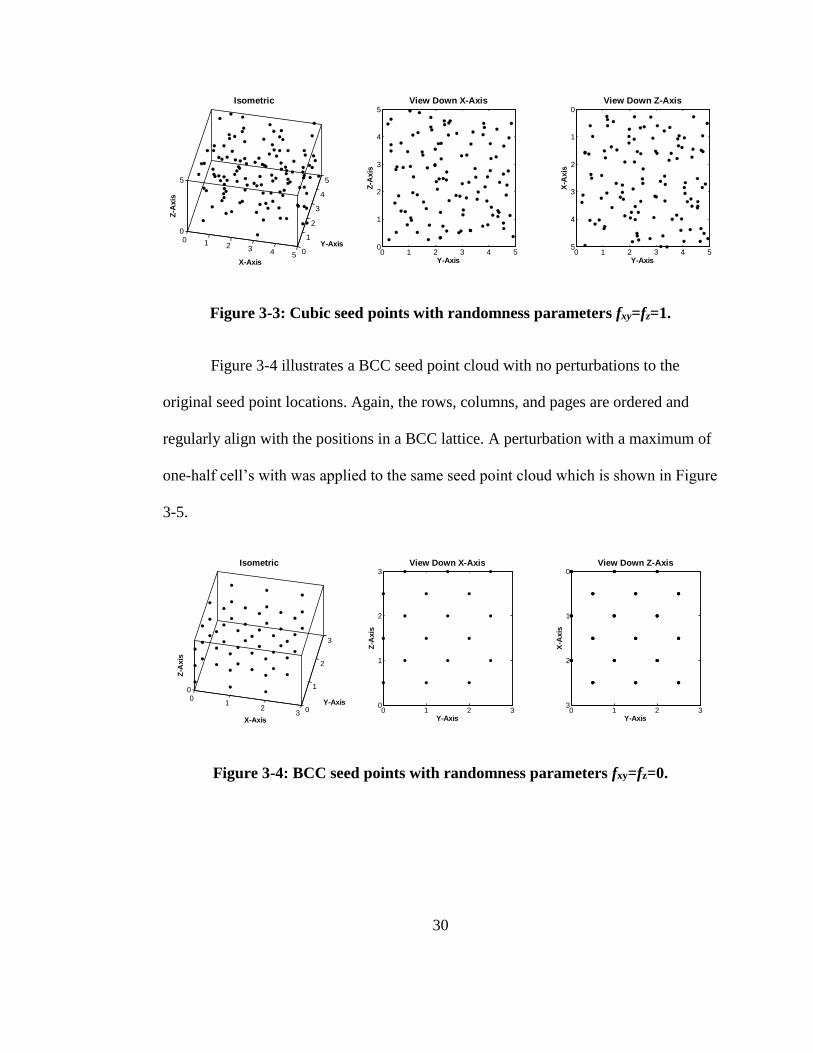
Figure 3-3: Cubic seed points with randomness parameters fxy=fz=1. ......................... 30

Figure 3-4: BCC seed points with randomness parameters fxy=fz=0. ........................... 30

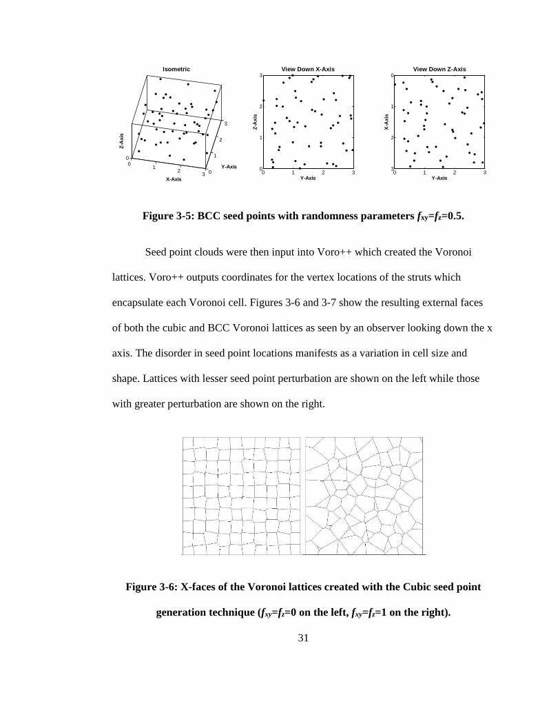
Figure 3-5: BCC seed points with randomness parameters fxy=fz=0.5. ........................ 31

Figure 3-6: X-faces of the Voronoi lattices created with the Cubic seed point

generation technique (fxy=fz=0 on the left, fxy=fz=1 on the right). ......................... 31

viii

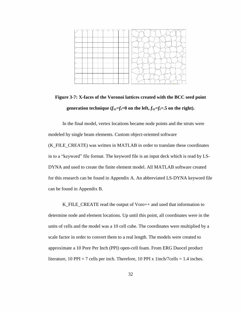
Figure 3-7: X-faces of the Voronoi lattices created with the BCC seed point generation

technique (fxy=fz=0 on the left, fxy=fz=.5 on the right). .......................................... 32

Figure 3-8: Visual representation of finite element model. ......................................... 35

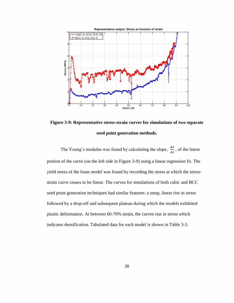
Figure 3-9: Representative stress-strain curves for simulations of two separate seed

point generation methods. .................................................................................... 38

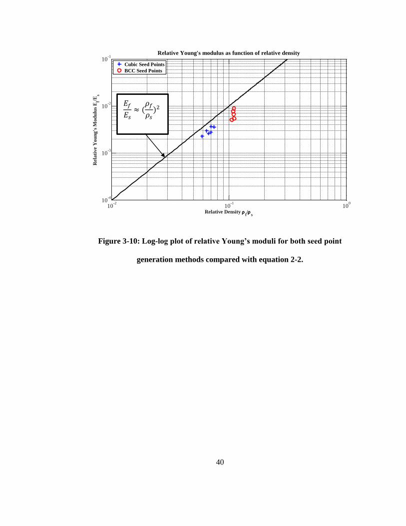
Figure 3-10: Log-log plot of relative Young’s moduli for both seed point generation

methods compared with equation 2-2. ................................................................. 40

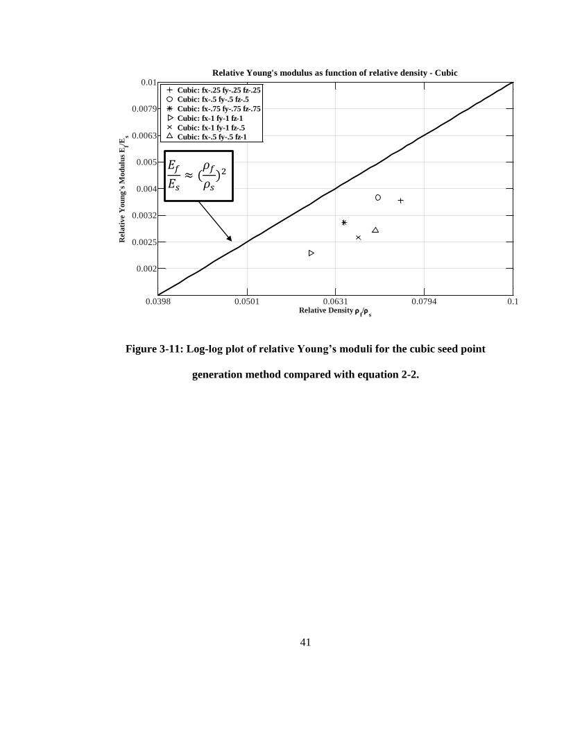
Figure 3-11: Log-log plot of relative Young’s moduli for the cubic seed point

generation method compared with equation 2-2. ................................................. 41

Figure 3-12: Log-log plot of relative Young’s moduli the BCC seed point generation

method compared with equation 2-2. ................................................................... 42

Figure 3-13: Log-log plot of relative yield strength for both seed point generation

methods compared with equation 2-3. ................................................................. 43

Figure 3-14: Log-log plot of relative yield strength for the cubic seed point generation


Figure 3-15 Log-log plot of relative yield strength for the cubic seed point generation


Figure 4-1: Force as function of time for all samples. ................................................. 50

Figure 4-2: Stress as function of strain for all samples. ............................................... 50

Figure 4-3: Force-time (left) and stress-strain (right) curves from sample .................. 52

Figure 4-4: Time-series of 10PPI-1 impact. Times are in seconds. ............................. 54

Figure 4-5: Time-series of 20PPI-1 impact. ................................................................. 55

ix

Figure 4-6: Time-series of 40PPI-2 impact. ................................................................. 56

Figure 5-1: Tensile sample dimensions. ...................................................................... 57

Figure 5-2: Tensile sample in sample holder. .............................................................. 58

Figure 5-3: Close-up of tensile sample epoxied into sample holder. ........................... 59

Figure 5-4: Photos of the tensile impactor. .................................................................. 59

Figure 5-5: Plot of force as function of time for both tensile experiments. ................. 61

Figure 5-6: Time-series photos from tensile experiment Test 1. ................................. 61

Figure 5-7: Time-series photos from tensile experiment Test 2. ................................. 62

Figure 5-8: Plot of stress as function of strain for both tensile experiments. .............. 63

Figure 6-1: Relative Young’s modulus as function of relative density comparison of

work from this thesis to previously published work. ........................................... 65

Figure 6-2: Relative Yield strength as function of relative density comparison of work

from this thesis to previously published work. .................................................... 66

Figure 6-3: Stress-strain curve from Gaitanaros, Kyriakides, and Kraynik (2012) ..... 67

Figure 6-4: Stress-strain curves from experimental and FEM data ............................. 67

Figure 6-5: Tensile stress-strain curve given by Andrews et al. (1999) ...................... 69

Figure 6-6: Experimental tensile stress-strain curve .................................................... 70

1

CHAPTER 1

INTRODUCTION

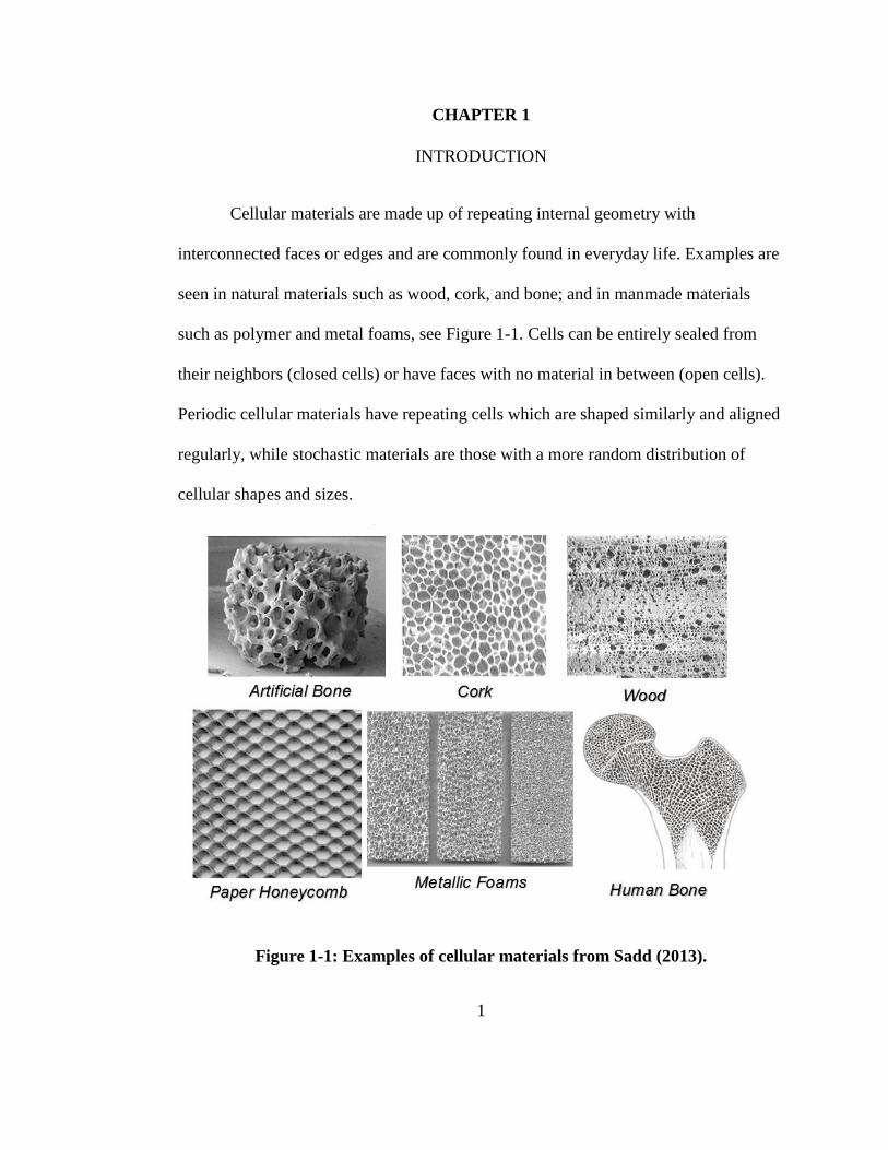
Cellular materials are made up of repeating internal geometry with

interconnected faces or edges and are commonly found in everyday life. Examples are

seen in natural materials such as wood, cork, and bone; and in manmade materials

such as polymer and metal foams, see Figure 1-1. Cells can be entirely sealed from

their neighbors (closed cells) or have faces with no material in between (open cells).

Periodic cellular materials have repeating cells which are shaped similarly and aligned

regularly, while stochastic materials are those with a more random distribution of

cellular shapes and sizes.

Figure 1-1: Examples of cellular materials from Sadd (2013).

2

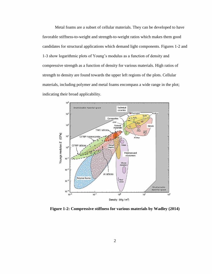
Metal foams are a subset of cellular materials. They can be developed to have

favorable stiffness-to-weight and strength-to-weight ratios which makes them good

candidates for structural applications which demand light components. Figures 1-2 and

1-3 show logarithmic plots of Young’s modulus as a function of density and

compressive strength as a function of density for various materials. High ratios of

strength to density are found towards the upper left regions of the plots. Cellular

materials, including polymer and metal foams encompass a wide range in the plot;

indicating their broad applicability.

Figure 1-2: Compressive stiffness for various materials by Wadley (2014)

3

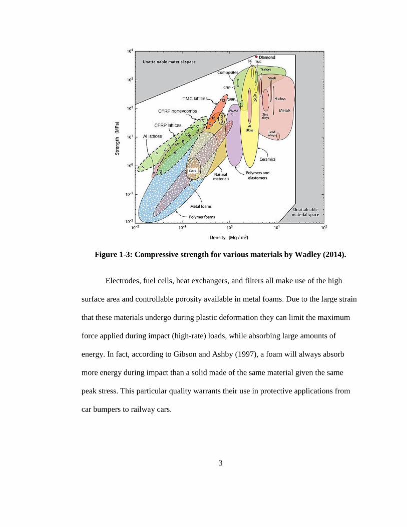
Figure 1-3: Compressive strength for various materials by Wadley (2014).

Electrodes, fuel cells, heat exchangers, and filters all make use of the high

surface area and controllable porosity available in metal foams. Due to the large strain

that these materials undergo during plastic deformation they can limit the maximum

force applied during impact (high-rate) loads, while absorbing large amounts of

energy. In fact, according to Gibson and Ashby (1997), a foam will always absorb

more energy during impact than a solid made of the same material given the same

peak stress. This particular quality warrants their use in protective applications from

car bumpers to railway cars.

4

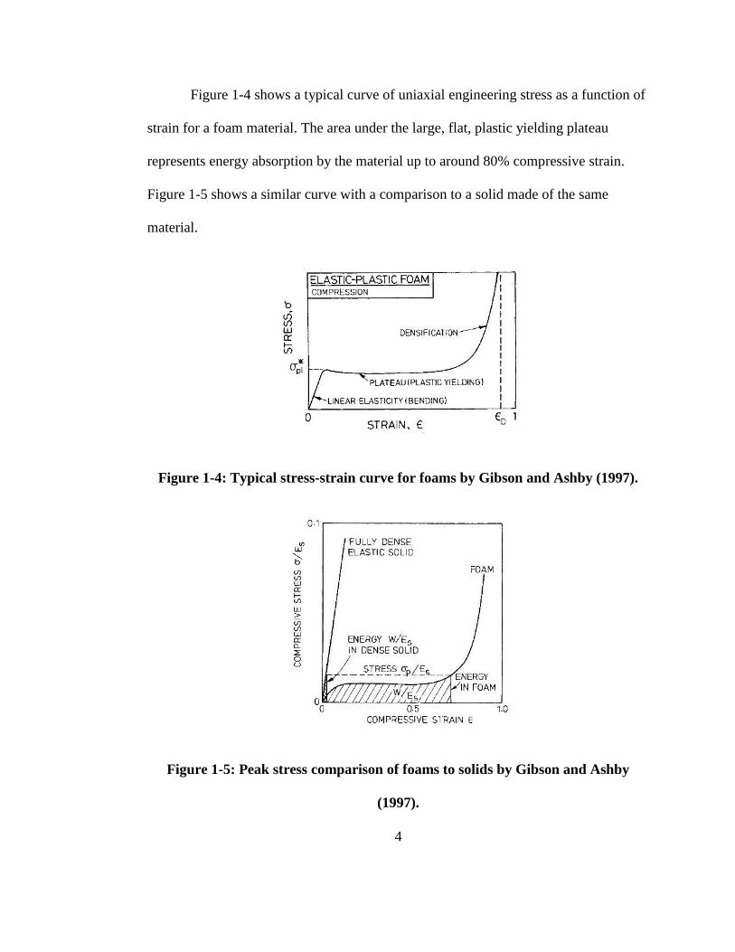
Figure 1-4 shows a typical curve of uniaxial engineering stress as a function of

strain for a foam material. The area under the large, flat, plastic yielding plateau

represents energy absorption by the material up to around 80% compressive strain.

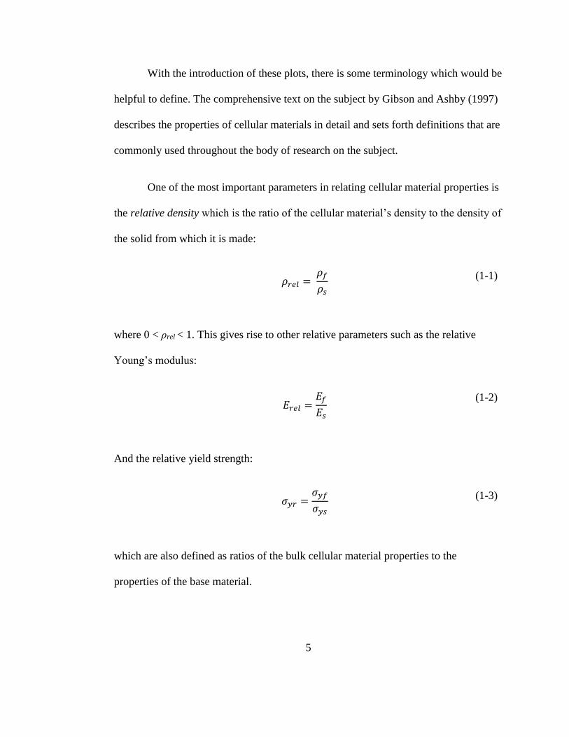
Figure 1-5 shows a similar curve with a comparison to a solid made of the same

material.

Figure 1-4: Typical stress-strain curve for foams by Gibson and Ashby (1997).

Figure 1-5: Peak stress comparison of foams to solids by Gibson and Ashby

(1997).

5

With the introduction of these plots, there is some terminology which would be

helpful to define. The comprehensive text on the subject by Gibson and Ashby (1997)

describes the properties of cellular materials in detail and sets forth definitions that are

commonly used throughout the body of research on the subject.

One of the most important parameters in relating cellular material properties is

the relative density which is the ratio of the cellular material’s density to the density of

the solid from which it is made:

𝜌𝑟𝑒𝑙 = 𝜌𝑓

𝜌𝑠

(1-1)

where 0 < ρrel < 1. This gives rise to other relative parameters such as the relative

Young’s modulus:

𝐸𝑟𝑒𝑙 =

𝐸𝑓

𝐸𝑠

(1-2)

And the relative yield strength:

𝜎𝑦𝑟 =𝜎𝑦𝑓

𝜎𝑦𝑠

(1-3)

which are also defined as ratios of the bulk cellular material properties to the

properties of the base material.

6

Similarly, since there are different stress and strain measures for materials

which undergo finite deformation, it is helpful to state that stress and strain in these

plots are generally reported in the literature as the engineering stress:

𝜎 =

𝐹

𝐴0

(1-4)

which is a ratio of the applied force to the original area of the foam; and the

engineering strain:

𝜀 =

∆𝐿

𝐿0

(1-5)

which is a ratio of the change in length of the foam to the original length. For the

remainder of this work, these will simply be referred to solely as stress and strain,

respectively.

In addition to these material parameters, several other properties of these plots

stand out. From left to right in Figure 1-4, it is noted that there are three distinct

regimes in which these foams behave: an elastic regime, in which stress as a function

of strain has a positive, nearly linear slope; a plastic yielding regime, in which stress is

mostly flat as strain increases; and a densification regime, in which a steep rise in

stress is noted as strain increases. The presence or absence of these regimes as well as

their description in relation to material properties will serve as guides in matching

material models to real world behavior.

7

Open-cell metal foams are made up of small metal ligaments. An example of

these foams is shown in Figure 1-6. Bubbles form in a molten metal mix which is then

cooled and hardened in to a porous media in which the ligaments form the new cell

boundaries.

Figure 1-6: A sample of Duocel ® open-cell aluminum foam.

The mathematical description of this process involves a random seeding of

points in a medium with subsequent nucleation and growth of bubbles about these

points. The boundary of each bubble encloses a volume in which all locations are

closer to the bubble’s original seed point than to any other. In two dimensions this

forms what is known mathematically as a Voronoi honeycomb. In three dimensions it

is a Voronoi foam. The terms “Voronoi lattice” and “Voronoi diagram” will also be

used interchangeably to describe this arrangement. Okabe et al. (1992) describes the

myriad applications of the Voronoi diagram including the description of particles in

8

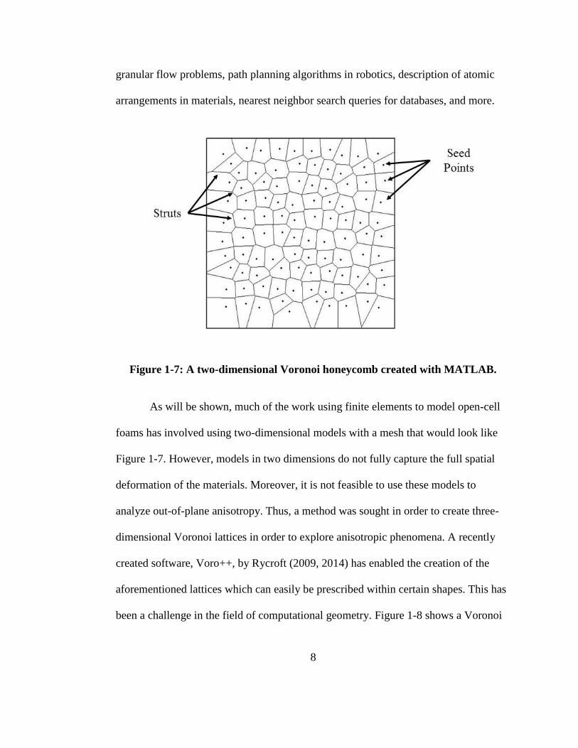
granular flow problems, path planning algorithms in robotics, description of atomic

arrangements in materials, nearest neighbor search queries for databases, and more.

Figure 1-7: A two-dimensional Voronoi honeycomb created with MATLAB.

As will be shown, much of the work using finite elements to model open-cell

foams has involved using two-dimensional models with a mesh that would look like

Figure 1-7. However, models in two dimensions do not fully capture the full spatial

deformation of the materials. Moreover, it is not feasible to use these models to

analyze out-of-plane anisotropy. Thus, a method was sought in order to create three-

dimensional Voronoi lattices in order to explore anisotropic phenomena. A recently

created software, Voro++, by Rycroft (2009, 2014) has enabled the creation of the

aforementioned lattices which can easily be prescribed within certain shapes. This has

been a challenge in the field of computational geometry. Figure 1-8 shows a Voronoi

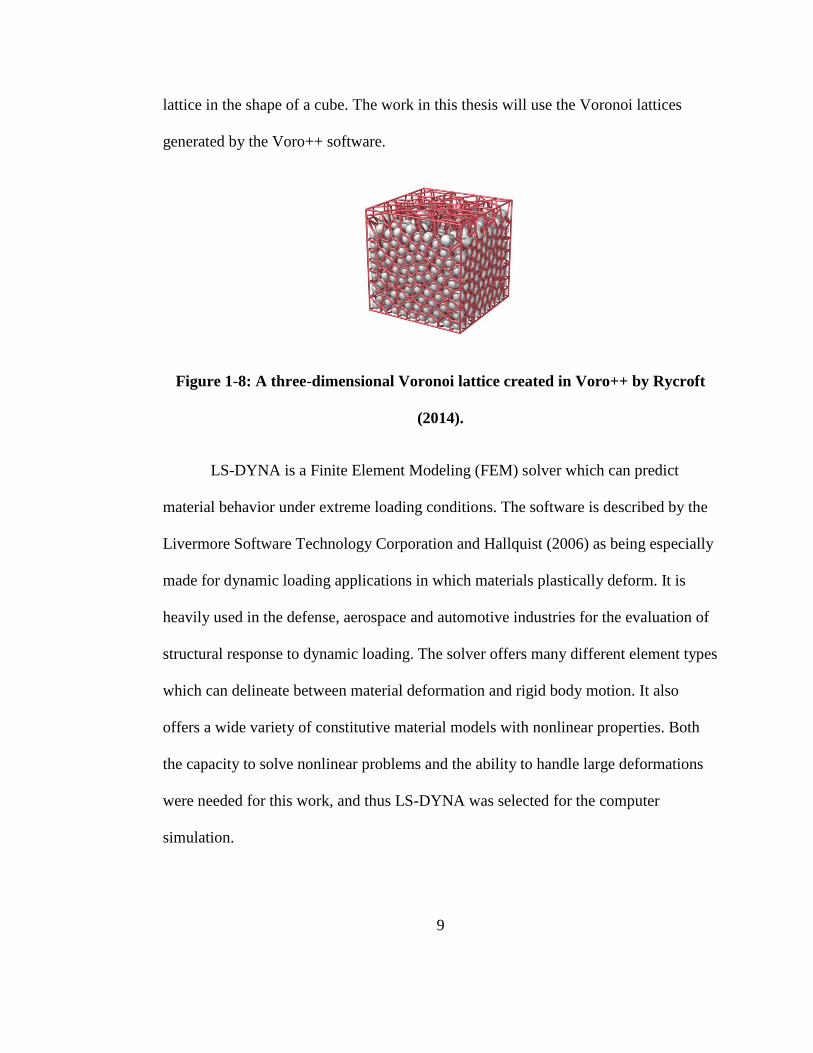
9

lattice in the shape of a cube. The work in this thesis will use the Voronoi lattices

generated by the Voro++ software.

Figure 1-8: A three-dimensional Voronoi lattice created in Voro++ by Rycroft

(2014).

LS-DYNA is a Finite Element Modeling (FEM) solver which can predict

material behavior under extreme loading conditions. The software is described by the

Livermore Software Technology Corporation and Hallquist (2006) as being especially

made for dynamic loading applications in which materials plastically deform. It is

heavily used in the defense, aerospace and automotive industries for the evaluation of

structural response to dynamic loading. The solver offers many different element types

which can delineate between material deformation and rigid body motion. It also

offers a wide variety of constitutive material models with nonlinear properties. Both

the capacity to solve nonlinear problems and the ability to handle large deformations

were needed for this work, and thus LS-DYNA was selected for the computer

simulation.

10

With increasing emphasis on efficiency and cost reductions, many impact-

absorption applications seek to reduce weight while maintaining or increasing energy

absorption during an impact event. Cellular materials, in particular open-cell metal

foams, offer advantages in this area and their response to dynamic loading has long

been studied. Recent mass-availability of 3D printing and surging interest in

advancing this technology have renewed attention to understanding the mechanical

response of these metal foams. The prospect of designing and building a material

which will increase energy absorption effectiveness in custom applications

necessitates in-depth understanding of the mechanisms by which these materials

deform.

This thesis has developed a highly adaptable and computationally efficient

finite element model which was used to explore the relation between foam parameters

and mechanical response in both linear (elastic) and nonlinear (elastic-plastic) load

regimes while under high-rate (dynamic) loading. This was accomplished by tying in

the three dimensional Voronoi lattices created in Voro++ with the LS-DYNA solver

which simulated large deformations and rate effects. In this way cellular porosity,

anisotropy, and shape/size distributions of open-cell foam material make-up was

controlled, observed, and altered. Drop-weight experiments, in which the open-cell

metal foams were dynamically loaded in compression and tension, were also

performed and photographed with a high speed camera. Data from the computational

material models were then compared with the experiments, previously published

11

research, and manufacturer’s specifications. This allowed for an evaluation of model

accuracy as well as for conclusions to be drawn as to how the aforementioned

properties affect dynamic material response.

With an understanding of the previous research on cellular materials it is

evident that a three-dimensional foam finite element model would add to the body of

research. Additionally, the absence of research on the response of open-cell foams to

tensile loading leads to interesting questions about such behavior. This work sought a

better understanding and exploration of the means by which open-cell foams deform

both in compression and tension. This adaptable model could then facilitate targeted

material design and creation.

12

CHAPTER 2

REVIEW OF LITERATURE

The mechanical behavior of metal foams has been well studied. Since initial

patents for methods to produce a “sponge metal” by Sosnik (1948) and “metal foam”

by Elliot (1951) these materials have been recognized as having unique properties.

According to ERG Aerospace Corporation (2014) open-cell metal foams were mostly

limited to military use until after the Cold War in the mid-1990s. Thus, the majority of

early work on metal foams was focused mainly on closed-cell materials. Since the

main definitions and many of the parameters still apply to open-cell materials, this

early research is still a good place to begin.

Initial studies by Thornton and Magee (1975) of closed-cell aluminum foams

in the 5-18% relative density range at strain rates of 8x10-3/s observe that a “greater

than linear” increase in yield strength occurs with increase in density. This leads them

to conclude that bending stresses within the foams are important mechanisms of

plastic collapse. They report an energy-absorbing efficiency parameter which is given

by:

𝑃 = ∫ 𝐹𝑑𝑙

𝑙

0

𝐹𝑚𝑎𝑥𝐿

(2-1)

where F is the instantaneous force which is then integrated over the distance of the

deformation, Fmax is the maximum force during the deformation, and L is the total

13

length of the deformed sample. Further, they concluded from their analysis that a more

regular cell structure would improve energy absorption. This work was also reported

by Davies and Zhen (1983) along with the description of manufacturing techniques to

create various types of foams in four different categories: casting, metallic deposition,

powder metallurgy, and sputter deposition. Along with methods of fabrication they

discuss the benefits and drawbacks of metallic foams in various applications. The

work concluded that impact absorption would be the application in which metal foams

have the greatest possibility for use.

The work by Ashby (1983) went in to great detail to describe the elastic,

plastic, creep, and fracture properties of cellular solids (mostly polymeric foams, but

Thornton and Magee’s work is included as well as some ceramic foams). Many of the

original figures and results from the experimental/analytical work are seen in the

second edition of the textbook, by Gibson and Ashby (1997). Although primarily

regarding nonmetallic foams, Ashby’s work sets forth a number of different

definitions and parameter relations which are used throughout the body of research on

the subject. Relative density and relative yield strength are two such parameters.

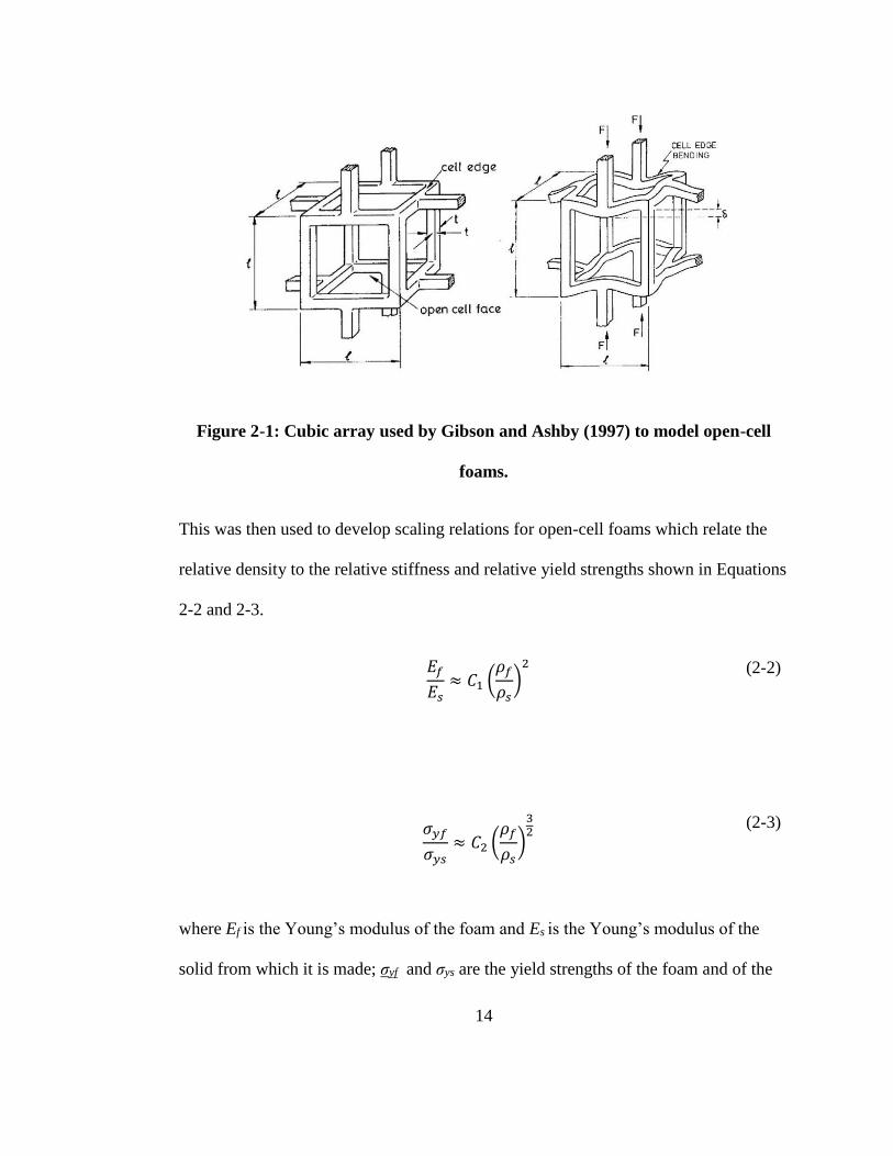
Gibson and Ashby then modeled an open-cell foam as the cubic array of struts

shown in Figure 2-1. Dimensional arguments were used to generalize the cell

properties without regard to specific cell geometry. The dimensional arguments

combined the cell size, l; the ligament thickness, t; with Timoshenko beam theory to

find the deflection, δ, as a function of F.

14

Figure 2-1: Cubic array used by Gibson and Ashby (1997) to model open-cell

foams.

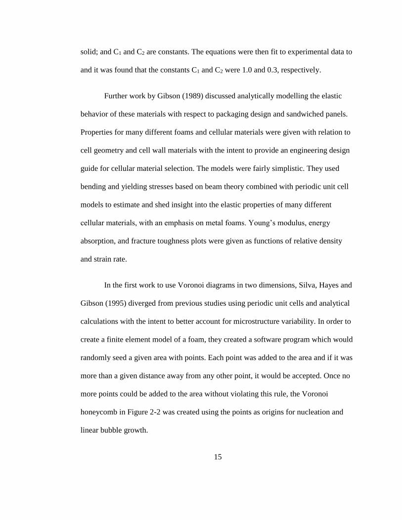
This was then used to develop scaling relations for open-cell foams which relate the

relative density to the relative stiffness and relative yield strengths shown in Equations

2-2 and 2-3.

𝐸𝑓

𝐸𝑠≈ 𝐶1 (

𝜌𝑓

𝜌𝑠)

2

(2-2)

𝜎𝑦𝑓

𝜎𝑦𝑠≈ 𝐶2 (

𝜌𝑓

𝜌𝑠)

32

(2-3)

where Ef is the Young’s modulus of the foam and Es is the Young’s modulus of the

solid from which it is made; σyf and σys are the yield strengths of the foam and of the

15

solid; and C1 and C2 are constants. The equations were then fit to experimental data to

and it was found that the constants C1 and C2 were 1.0 and 0.3, respectively.

Further work by Gibson (1989) discussed analytically modelling the elastic

behavior of these materials with respect to packaging design and sandwiched panels.

Properties for many different foams and cellular materials were given with relation to

cell geometry and cell wall materials with the intent to provide an engineering design

guide for cellular material selection. The models were fairly simplistic. They used

bending and yielding stresses based on beam theory combined with periodic unit cell

models to estimate and shed insight into the elastic properties of many different

cellular materials, with an emphasis on metal foams. Young’s modulus, energy

absorption, and fracture toughness plots were given as functions of relative density

and strain rate.

In the first work to use Voronoi diagrams in two dimensions, Silva, Hayes and

Gibson (1995) diverged from previous studies using periodic unit cells and analytical

calculations with the intent to better account for microstructure variability. In order to

create a finite element model of a foam, they created a software program which would

randomly seed a given area with points. Each point was added to the area and if it was

more than a given distance away from any other point, it would be accepted. Once no

more points could be added to the area without violating this rule, the Voronoi

honeycomb in Figure 2-2 was created using the points as origins for nucleation and

linear bubble growth.

16

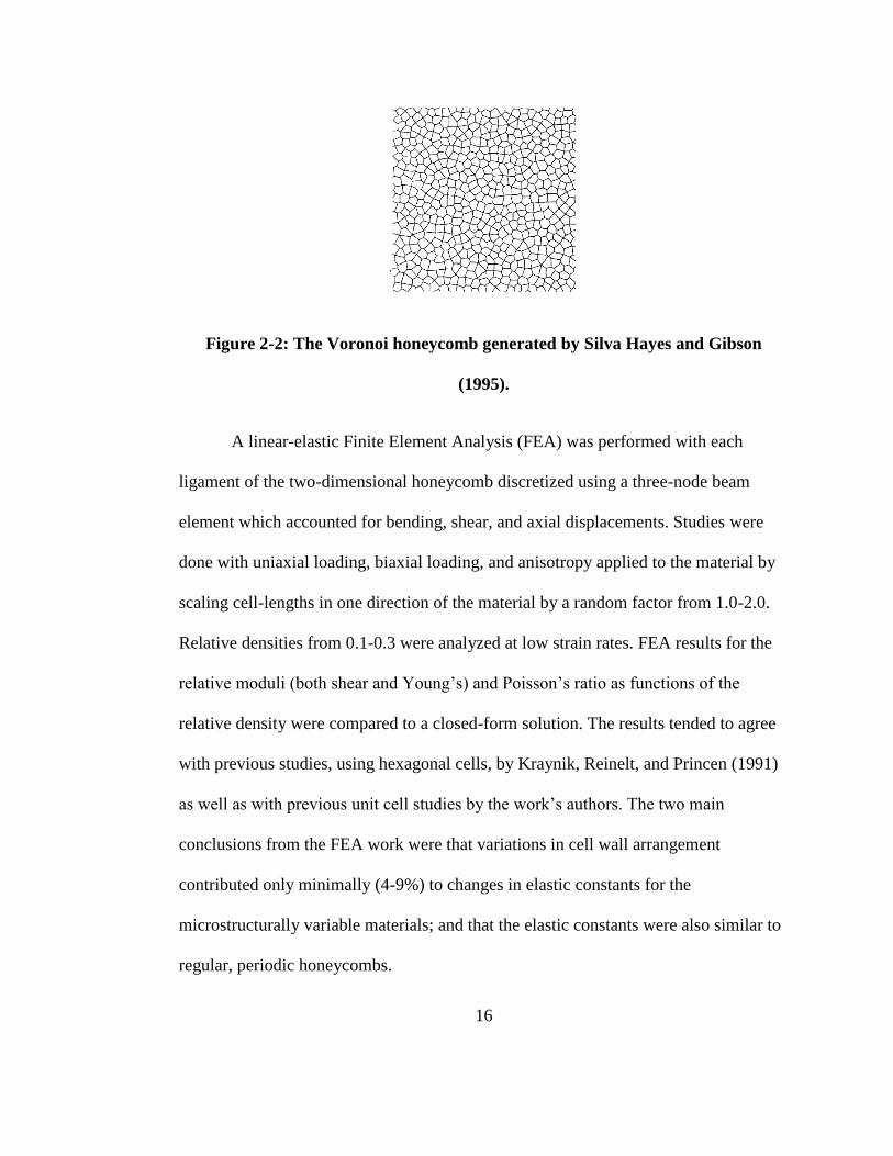
Figure 2-2: The Voronoi honeycomb generated by Silva Hayes and Gibson

(1995).

A linear-elastic Finite Element Analysis (FEA) was performed with each

ligament of the two-dimensional honeycomb discretized using a three-node beam

element which accounted for bending, shear, and axial displacements. Studies were

done with uniaxial loading, biaxial loading, and anisotropy applied to the material by

scaling cell-lengths in one direction of the material by a random factor from 1.0-2.0.

Relative densities from 0.1-0.3 were analyzed at low strain rates. FEA results for the

relative moduli (both shear and Young’s) and Poisson’s ratio as functions of the

relative density were compared to a closed-form solution. The results tended to agree

with previous studies, using hexagonal cells, by Kraynik, Reinelt, and Princen (1991)

as well as with previous unit cell studies by the work’s authors. The two main

conclusions from the FEA work were that variations in cell wall arrangement

contributed only minimally (4-9%) to changes in elastic constants for the

microstructurally variable materials; and that the elastic constants were also similar to

regular, periodic honeycombs.

17

Three-dimensional foam models started appearing with a study by Roberts and

Garboczi (2002) which used a three-dimensional finite element model to study the

dependence of Young’s modulus on relative density. At the time the work was done,

many theoretical models were using periodic cellular structures. Their research noted

that a gap existed between the understanding of these periodic models and the

behavior of real world cellular solids which have more random makeups. They used

Voronoi tessellations similar to the present study; models in which layers of the

material have a Gaussian density distribution; and nearest neighbor node-bonded

foams. They found that Young’s modulus was proportional to the density of the foam

to the power of n, where n is between 1.3 and 3.0.

Additional three-dimensional models using the finite element method were

created by Gan, Chen, and Shen (2005). Their work developed a three-dimensional

Voronoi finite element model which was then used to explore the mechanical response

of open-cell polymeric foams in the 1 to 10% relative density range. However, the

work focused only on the linear elastic response of the foams and thus diverged from

the present study. The Voronoi lattices were compared with a more-regular Kelvin

formulation proposed by Warren and Kraynik (1997) which was comprised of regular

tetrakaidecahedra (14-sided cells in a BCC lattice arrangement). The model by Gan,

Chen, and Shen model consisted of analyzing the response of N x N x N Voronoi cell

unit blocks (N = 3,4,5, and 6) and then adding them together to create a “super cell”

model of ultimate dimensions 3N x 3N x 3N cells. The calculated relative Young’s

18

moduli results for N = 3 and N = 5 models differed by less than 10%. They found that

the elastic constants predicted by Voronoi and Kelvin foams for low density open-cell

foams were in close agreement, but diverged as relative density increased. In addition,

they concluded that Young’s modulus of Voronoi foams was sensitive to

imperfections in the foam lattice, while the plateau stress of the foams was not.

More recent work has focused on using greater cellular variations in two-

dimensional finite element models of Voronoi tessellations to further explore

microstructural effects. Alkhader and Vural (2006, 2008) used models of this type to

link cellular microstructure with material response in both the quasistatic and dynamic

load regimes. Their work focused on characterizing what role specimen size, boundary

morphology, cellular topology, and microstructural irregularity have on the

mechanical response of two-dimensional foams. These studies looked at similar

methods of generating nucleation points for the Voronoi tessellation as the

aforementioned study by Silva et al. It also used a second method which began with a

point grid and then added random perturbations to the points in the grid (this method is

ultimately chosen by the current work). Between 2 and 7 Timoshenko beam elements

were used to discretize each ligament in the foam models which had relative densities

in the range of 15%. In the quasistatic study, a displacement boundary condition was

set at the top of the specimen, enforcing a 1/s strain rate. The dynamic study by

Alkhader and Vural set up the FE model similarly, but with a strain rate of 1000/s. The

models looked at several sample sizes (in numbers of cells), shapes (pure Voronoi,

19

tetragonal, hexagonal), and perturbations to the nucleation points in the foam. The

authors made several conclusions with direct applicability to the work herein. First,

they found that the response of the models was most accurately modeled at a size of at

least 10 x 10 cells. Next, they concluded that the arrangement of cells around the

boundaries had little effect on compressive response, but boundary conditions did

have a significant effect. Lastly, with respect to microstructure, they found that a loss

of periodicity can contribute to bending-dominated structural response which, in turn,

leads to slight decrease in macroscopic stiffness. These conclusions hold true for both

the quasistatic and dynamic loading scenarios. A unique conclusion for the dynamic

load scenario was that the simulations suggested a strong sensitivity to load rates, with

particular emphasis on the rise time of initial loading. They suggest that more study

should be tuned to investigating appropriate rise times in dynamic simulations of

cellular materials.

The idea of “functionally graded materials” for enhanced properties was

explored by Ajdari et al. (2009) in the quasistatic loading case and again by Ajdari et

al. (2011) to look at tailored microstructure’s effects on dynamic crushing properties.

The 2009 study created a finite element model with a two-dimensional Voronoi

honeycomb in a similar way to the previously mentioned studies: using beam elements

in SIMULIA (formerly ABAQUS). Between 2 and 6 elements were used for each

ligament. Beam materials were linear elastic and elastic-perfectly plastic for the elastic

and elastic-plastic load regimes, respectively; with constants which mimicked

20

properties of aluminum. The authors diverged from previous studies by simulating a

material with a relative density that varied spatially from 10% increasing along the

loading direction to a peak density of 53% at the surface to which the load was

applied. Results were compared to a sample with 10% constant density. The work

concluded that the increasing density gradient increased both the material’s stiffness

and yield stress, but had a more pronounced effect on the former. The 2011 Adjari

work used regular, periodic honeycomb models with similar computational inputs and

explored dynamic scenarios. Although the exact strain rates imposed in the research

were unclear, the research found that a decreasing gradient in the load direction

increased the energy absorption in early stages of crushing.

Jones (2011) studied the effect that topology has on the stress intensification

around a circular hole. The work used a two-dimensional Voronoi honeycomb to

explore these effects and found that reducing the hole size resulted in a reduction of

the stress amplification at the corners, which is the opposite effect found in solid

materials. Additionally, the research found that by optimizing relative density

distribution to align with areas in the material in which high stresses were present a

global reduction in material stresses could be achieved. Breault (2012) expanded on

this finding by aligning the topology (struts and ligaments) of a cellular material with

stress trajectories found in the continuum material. The Breault research found that

alignment of the struts according to stress trajectories lowered both maximum and

average stresses found in the material.

21

Although many efforts to model open-cell foams have involved finite element

models of semi-randomly generated networks of beam elements, some research has

actually tried to exactly match specific samples and then model them. One such

example is from Liebscher et al. (2012) who used X-ray computed tomography to scan

a material sample. This data was then used to create a finite element model consisting

of Timoshenko beams to predict material response to vibrations.

An experimental work by Tan, Reid, and Harrigan (2012) examined how the

structural response of cell walls in open-cell metal foams is affected by the anisotropy

of cell shape. They further investigated how this alteration of cell shape would affect

crush patterns and the mechanical properties while the materials are subjected to

dynamic loads. The experiments looked at open-cell aluminum foams of 6106-T6

Alumininum in the 9-10% relative density range with porosities of 10 and 40 pores-

per-inch. The foams were compressed at strain rates from 400/s to 4,000/s. The

deformation and crush patterns in the materials are shown to be functions of the load

rate. These patterns fit into regimes which are delineated by critical impact velocities

at which the deformation patterns are observed to change (the border between the

“sub-critical” and “super-critical” load regimes is around 2300/s).

The work concludes that in the sub-critical regime, translational and rotational

inertia of the cell ligaments contribute to strength enhancement and the plastic

collapse strength increases linearly with load rate. However, in the super-critical load

regime, the plastic collapse strength is a function of the square of the impact velocity.

22

They conclude that this change is based on shock propagation effects. This cell

ligament motion is termed “microinertia”. The experiments are compared with

previously conducted two-dimensional finite element simulations. Notably, the work

investigates the effects of the anisotropy of the foam cells. Samples were observed to

have cells which were slightly oblong. Strength and plateau stress were shown to

decrease when the load was aligned perpendicular to the longer axis of the cells.

Finite element studies which have analyzed three-dimensional Voronoi lattices

under dynamic loads are rare, this is most likely due to the complexity in creating a

three-dimensional Voronoi lattice as well as the large computational requirements in

analyzing it. Very recent work by Gaitanaros, Kyriakides, and Kraynik (2012), and

Gaitanaros and Kyriakides (2013), have studied this behavior. Their research closely

parallels the work herein in its use of the LS-DYNA numerical solver and a lattice

which departs from previously studies in that varying cell size is accounted for. The

2012 work by Gaitanaros, et al. creates a soap froth using a software created by called

Surface Evolver. The creator, Brakke (1992) describes it as a software which can

model the shape that liquid surfaces take in response to various forces. The froth is

reduced to a set of ligaments through an algorithm which minimizes the surface

energy of the bubbles in the froth (similarly to how real open-cell foams form). This

gives the model the ability to vary cross-section diameter along ligament length. Each

ligament is discretized in great detail by 7-9 beam Hughes-Liu (1981) beam elements,

depending on the length of the ligament. The Hughes-Liu beam element accounts for

23

finite deformations, rotations, and shear and has the capability to account for and

apply friction to contact between beam elements. The authors looked at the

relationship between the model size (in cell dimensions) and convergence. The models

were shown to converge at around 1,000 cells (a 10 x 10 x 10-cell cube) which is in

general agreement with previous two-dimensional finite element models.

Foams in the 8% density range were first modeled under quasistatic conditions

in the Gaitanaros, Kyriakides, and Kraynik’s 2012 study and then under dynamic

conditions in Gaitanaros and Kyriakides’s 2013 study. Strain rates in each study were

0.1/s and 800-8000/s, respectively. Models were shown to exhibit many of the same

physical phenomena (crush zones, densification, and large plastic deformation) as real

foams.

The current study seeks a more flexible tool with which to model open-cell

foams. The forces of nature (surface forces in molten aluminum slurries) currently

drive the ability to control the porosity and microstructure of these foams. However,

with the advances in additive manufacturing it is easy to imagine a future in which

these foams can be designed and then formed in ways which would not be possible

with present manufacturing technologies. Cells and ligaments can take more varied

shapes; their sizes and anisotropy can be controlled. An open-cell foam could

conceivably be designed and built ligament by ligament with a specific purpose in

mind. In order to do this, foam models will need to be more easily adaptable and

controllable. The present work seeks to build upon this concept.

24

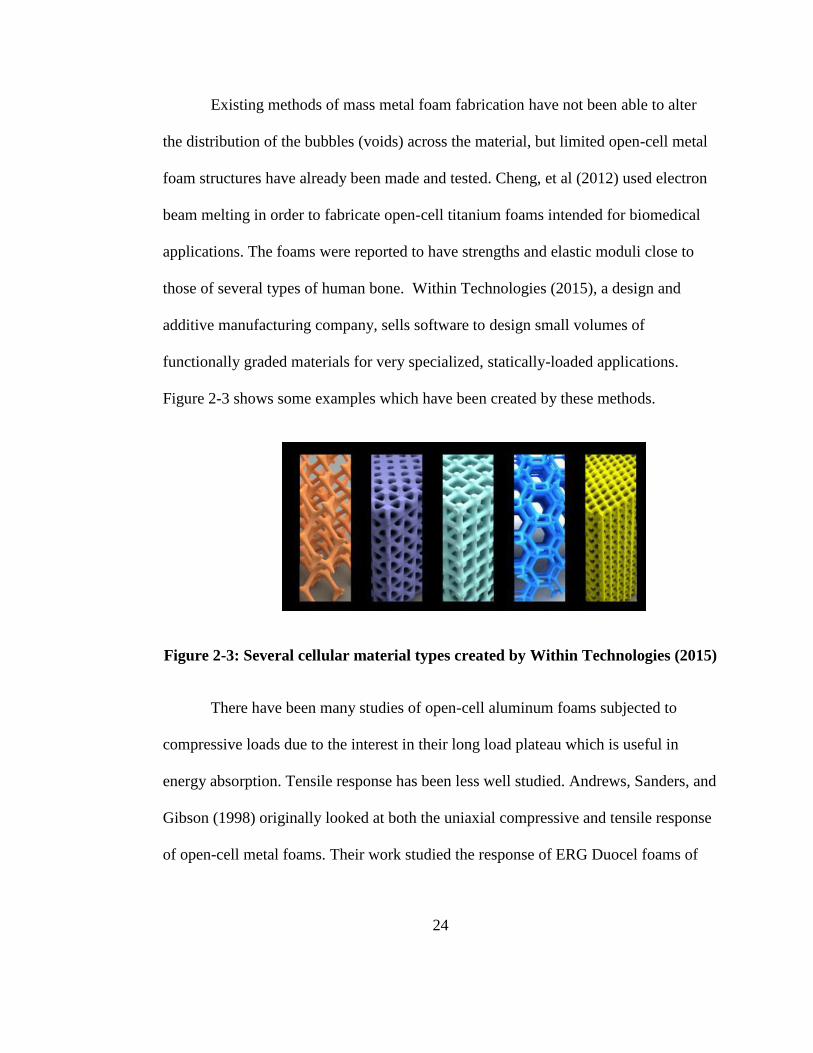
Existing methods of mass metal foam fabrication have not been able to alter

the distribution of the bubbles (voids) across the material, but limited open-cell metal

foam structures have already been made and tested. Cheng, et al (2012) used electron

beam melting in order to fabricate open-cell titanium foams intended for biomedical

applications. The foams were reported to have strengths and elastic moduli close to

those of several types of human bone. Within Technologies (2015), a design and

additive manufacturing company, sells software to design small volumes of

functionally graded materials for very specialized, statically-loaded applications.

Figure 2-3 shows some examples which have been created by these methods.

Figure 2-3: Several cellular material types created by Within Technologies (2015)

There have been many studies of open-cell aluminum foams subjected to

compressive loads due to the interest in their long load plateau which is useful in

energy absorption. Tensile response has been less well studied. Andrews, Sanders, and

Gibson (1998) originally looked at both the uniaxial compressive and tensile response

of open-cell metal foams. Their work studied the response of ERG Duocel foams of

25

8% relative density and10 PPI in the .0002/s strain rate regime. They published the

Young’s modulus and yield strength of the foams to be .502 GPa and 1.93 MPa,

respectively. They compared the response of open-cell foams to an analytical model

and found good agreement. In contrast, they found that closed-cell foams were not

well described by this model which they attributed to imperfections in the metal which

made up the cell walls. Related tensile work was performed by Olurin, Fleck, and

Ashby (2000) on closed-cell foams in the 8-15% relative density range at strain rates

of .00017/s and found that the foams exhibited strain hardening and failed in the range

of 1-3% strain. Scatter in their sample response data lead them to conclusions which

generally agreed with those of Andrews et al in that the samples had heterogeneous

microstructure and imperfections.

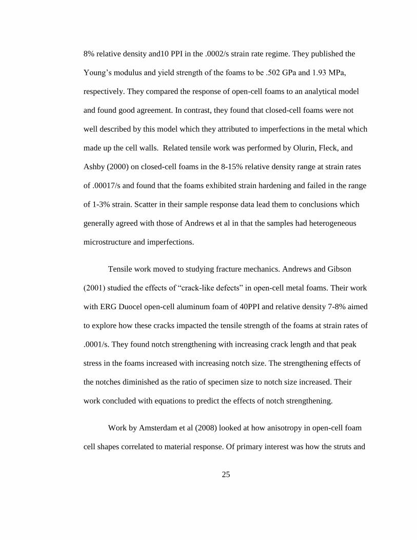
Tensile work moved to studying fracture mechanics. Andrews and Gibson

(2001) studied the effects of “crack-like defects” in open-cell metal foams. Their work

with ERG Duocel open-cell aluminum foam of 40PPI and relative density 7-8% aimed

to explore how these cracks impacted the tensile strength of the foams at strain rates of

.0001/s. They found notch strengthening with increasing crack length and that peak

stress in the foams increased with increasing notch size. The strengthening effects of

the notches diminished as the ratio of specimen size to notch size increased. Their

work concluded with equations to predict the effects of notch strengthening.

Work by Amsterdam et al (2008) looked at how anisotropy in open-cell foam

cell shapes correlated to material response. Of primary interest was how the struts and

26

ligaments bend and reorient themselves when foams are subjected to an applied strain.

The ERG Duocel open-cell Aluminum foam of 20PPI and relative density 3-13% were

Electro-Discharge Machined (EDM) and strained at .0019/s strain rate. They found

that strain hardening in the foams was unaffected by cell orientation and that a higher

peak strain is obtained in the foams when the long axis of the sample was oriented

transverse to the loading axis. They attributed this to an increase in the contribution of

strut bending to the foam mechanical response.

27

CHAPTER 3

FINITE ELEMENT MODELING

3.1 Preliminaries

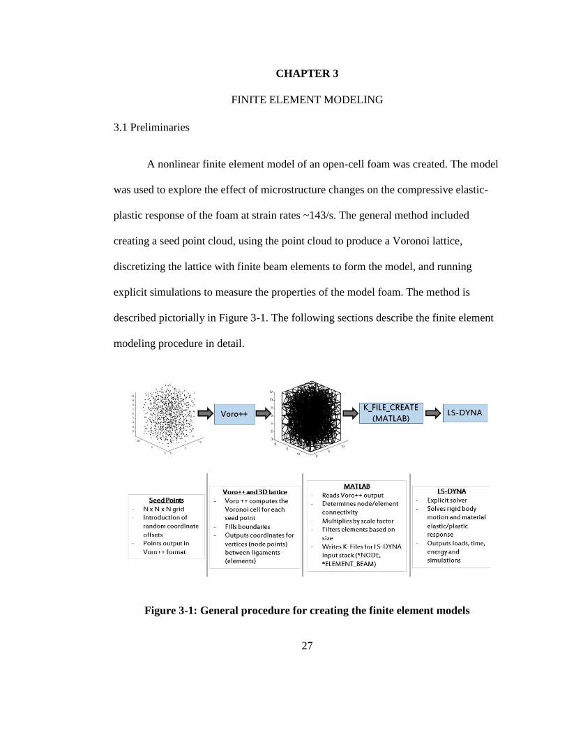
A nonlinear finite element model of an open-cell foam was created. The model

was used to explore the effect of microstructure changes on the compressive elastic-

plastic response of the foam at strain rates ~143/s. The general method included

creating a seed point cloud, using the point cloud to produce a Voronoi lattice,

discretizing the lattice with finite beam elements to form the model, and running

explicit simulations to measure the properties of the model foam. The method is

described pictorially in Figure 3-1. The following sections describe the finite element

modeling procedure in detail.

Figure 3-1: General procedure for creating the finite element models

28

3.2 Seed Point Generation, Pseudo-Randomization, and Voronoi Lattice Computation

Two methods for creating the Voronoi seed points were explored: the “Cubic”

method, and the “Body-Centered Cubic” or BCC method. Each of these methods were

taken from natural crystallographic atomic packing arrangements. Attempts were

made to produce Face-Centered Cubic (FCC) and Hexagonal Close-Packed (HCP)

seed points, but each resulted in dense packing which produced too many elements for

the element-limited version of LS-DYNA which was obtained.

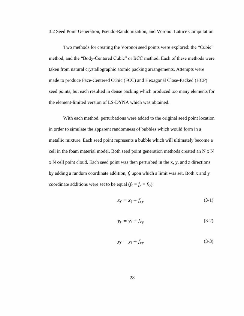
With each method, perturbations were added to the original seed point location

in order to simulate the apparent randomness of bubbles which would form in a

metallic mixture. Each seed point represents a bubble which will ultimately become a

cell in the foam material model. Both seed point generation methods created an N x N

x N cell point cloud. Each seed point was then perturbed in the x, y, and z directions

by adding a random coordinate addition, f, upon which a limit was set. Both x and y

coordinate additions were set to be equal (fx = fy = fxy):

𝑥𝑓 = 𝑥𝑖 + 𝑓𝑥𝑦 (3-1)

𝑦𝑓 = 𝑦𝑖 + 𝑓𝑥𝑦 (3-2)

𝑦𝑓 = 𝑦𝑖 + 𝑓𝑥𝑦 (3-3)

29

in which xi, yi, zi are the x,y,z coordinates of the original seed points created in both

the cubic and BCC lattices. The value for f was chosen to be from zero to one full

cell’s width in the cubic seed point generation technique and from 0 to one-half cell’s

width in the BCC seed point generation technique. Due to the half-cell spacing of the

BCC points, they could not be moved one full cell as that would shift the seed points

to a new position. Figures 3-2 through 3-5 show seed point clouds for some specific

cases.

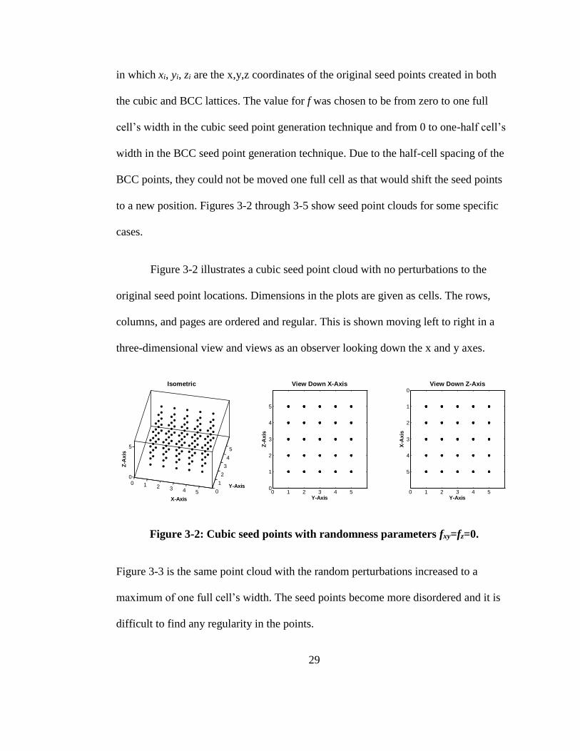
Figure 3-2 illustrates a cubic seed point cloud with no perturbations to the

original seed point locations. Dimensions in the plots are given as cells. The rows,

columns, and pages are ordered and regular. This is shown moving left to right in a

three-dimensional view and views as an observer looking down the x and y axes.

Figure 3-2: Cubic seed points with randomness parameters fxy=fz=0.

Figure 3-3 is the same point cloud with the random perturbations increased to a

maximum of one full cell’s width. The seed points become more disordered and it is

difficult to find any regularity in the points.

0 1 2 3 4 5 0

1

2

3

4

5

0

5

Z-A

xis

Isometric

X-Axis

Y-Axis0 1 2 3 4 5

0

1

2

3

4

5

View Down X-Axis

Z-A

xis

Y-Axis

0

1

2

3

4

5

0 1 2 3 4 5

View Down Z-Axis

X-A

xis

Y-Axis

30

Figure 3-3: Cubic seed points with randomness parameters fxy=fz=1.

Figure 3-4 illustrates a BCC seed point cloud with no perturbations to the

original seed point locations. Again, the rows, columns, and pages are ordered and

regularly align with the positions in a BCC lattice. A perturbation with a maximum of

one-half cell’s with was applied to the same seed point cloud which is shown in Figure

3-5.

Figure 3-4: BCC seed points with randomness parameters fxy=fz=0.

0 1 2 3 4 5 0

1

2

3

4

5

0

5

Y-Axis

X-Axis

Isometric

Z-A

xis

0 1 2 3 4 50

1

2

3

4

5View Down X-Axis

Y-Axis

Z-A

xis

0

1

2

3

4

50 1 2 3 4 5

View Down Z-Axis

Y-Axis

X-A

xis

01

23 0

1

2

3

0

Z-A

xis

Isometric

X-Axis

Y-Axis0 1 2 3

0

1

2

3View Down X-Axis

Z-A

xis

Y-Axis

0

1

2

30 1 2 3

View Down Z-AxisX

-Axis

Y-Axis

31

Figure 3-5: BCC seed points with randomness parameters fxy=fz=0.5.

Seed point clouds were then input into Voro++ which created the Voronoi

lattices. Voro++ outputs coordinates for the vertex locations of the struts which

encapsulate each Voronoi cell. Figures 3-6 and 3-7 show the resulting external faces

of both the cubic and BCC Voronoi lattices as seen by an observer looking down the x

axis. The disorder in seed point locations manifests as a variation in cell size and

shape. Lattices with lesser seed point perturbation are shown on the left while those

with greater perturbation are shown on the right.

Figure 3-6: X-faces of the Voronoi lattices created with the Cubic seed point

generation technique (fxy=fz=0 on the left, fxy=fz=1 on the right).

01

23 0

1

2

3

0

Y-Axis

X-Axis

Isometric

Z-A

xis

0 1 2 30

1

2

3View Down X-Axis

Y-Axis

Z-A

xis

0

1

2

30 1 2 3

View Down Z-Axis

Y-Axis

X-A

xis

32

Figure 3-7: X-faces of the Voronoi lattices created with the BCC seed point

generation technique (fxy=fz=0 on the left, fxy=fz=.5 on the right).

In the final model, vertex locations became node points and the struts were

modeled by single beam elements. Custom object-oriented software

(K_FILE_CREATE) was written in MATLAB in order to translate these coordinates

in to a “keyword” file format. The keyword file is an input deck which is read by LS-

DYNA and used to create the finite element model. All MATLAB software created

for this research can be found in Appendix A. An abbreviated LS-DYNA keyword file

can be found in Appendix B.

K_FILE_CREATE read the output of Voro++ and used that information to

determine node and element locations. Up until this point, all coordinates were in the

units of cells and the model was a 10 cell cube. The coordinates were multiplied by a

scale factor in order to convert them to a real length. The models were created to

approximate a 10 Pore Per Inch (PPI) open-cell foam. From ERG Duocel product

literature, 10 PPI = 7 cells per inch. Therefore, 10 PPI x 1inch/7cells = 1.4 inches.

33

Since the models were in units of meters (m), kilograms (kg), seconds (s) this number

was multiplied by .0254 to equate the 10 cell cube to a model cube which was .036m

on a side. Prior to putting the final coordinates into keyword format, duplicate nodes

and elements were rejected as well as elements which were less than 0.1mm in length.

This was done to get rid of non-real elements as well as to expedite the finite element

simulation since the time step of an explicit analysis is determined by the shortest

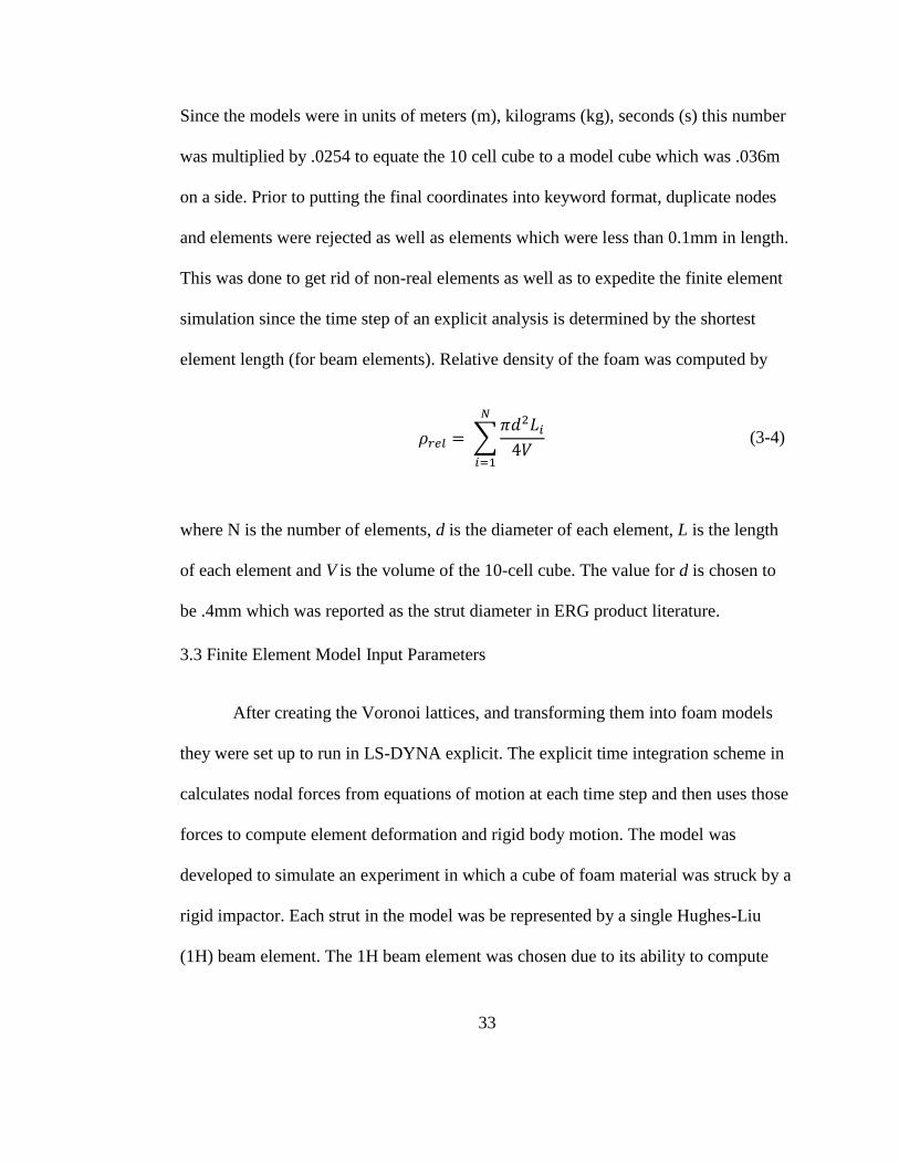
element length (for beam elements). Relative density of the foam was computed by

𝜌𝑟𝑒𝑙 = ∑𝜋𝑑2𝐿𝑖

4𝑉

𝑁

𝑖=1

(3-4)

where N is the number of elements, d is the diameter of each element, L is the length

of each element and V is the volume of the 10-cell cube. The value for d is chosen to

be .4mm which was reported as the strut diameter in ERG product literature.

3.3 Finite Element Model Input Parameters

After creating the Voronoi lattices, and transforming them into foam models

they were set up to run in LS-DYNA explicit. The explicit time integration scheme in

calculates nodal forces from equations of motion at each time step and then uses those

forces to compute element deformation and rigid body motion. The model was

developed to simulate an experiment in which a cube of foam material was struck by a

rigid impactor. Each strut in the model was be represented by a single Hughes-Liu

(1H) beam element. The 1H beam element was chosen due to its ability to compute

34

compression, tension, moment, and torsion. In addition, the 1H element reported

contact between elements and distinguished between element deflection and rigid

body motion.

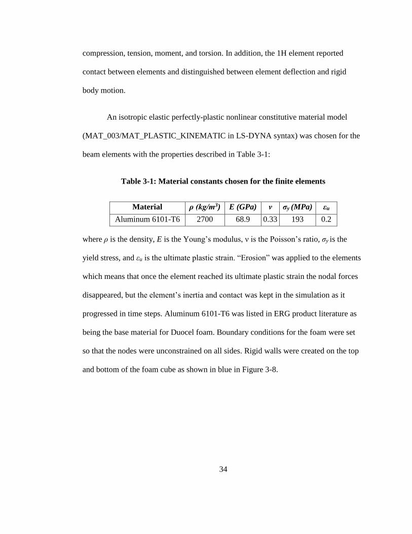
An isotropic elastic perfectly-plastic nonlinear constitutive material model

(MAT_003/MAT_PLASTIC_KINEMATIC in LS-DYNA syntax) was chosen for the

beam elements with the properties described in Table 3-1:

Table 3-1: Material constants chosen for the finite elements

Material ρ (kg/m3) E (GPa) ν σy (MPa) εu

Aluminum 6101-T6 2700 68.9 0.33 193 0.2

where ρ is the density, E is the Young’s modulus, ν is the Poisson’s ratio, σy is the

yield stress, and εu is the ultimate plastic strain. “Erosion” was applied to the elements

which means that once the element reached its ultimate plastic strain the nodal forces

disappeared, but the element’s inertia and contact was kept in the simulation as it

progressed in time steps. Aluminum 6101-T6 was listed in ERG product literature as

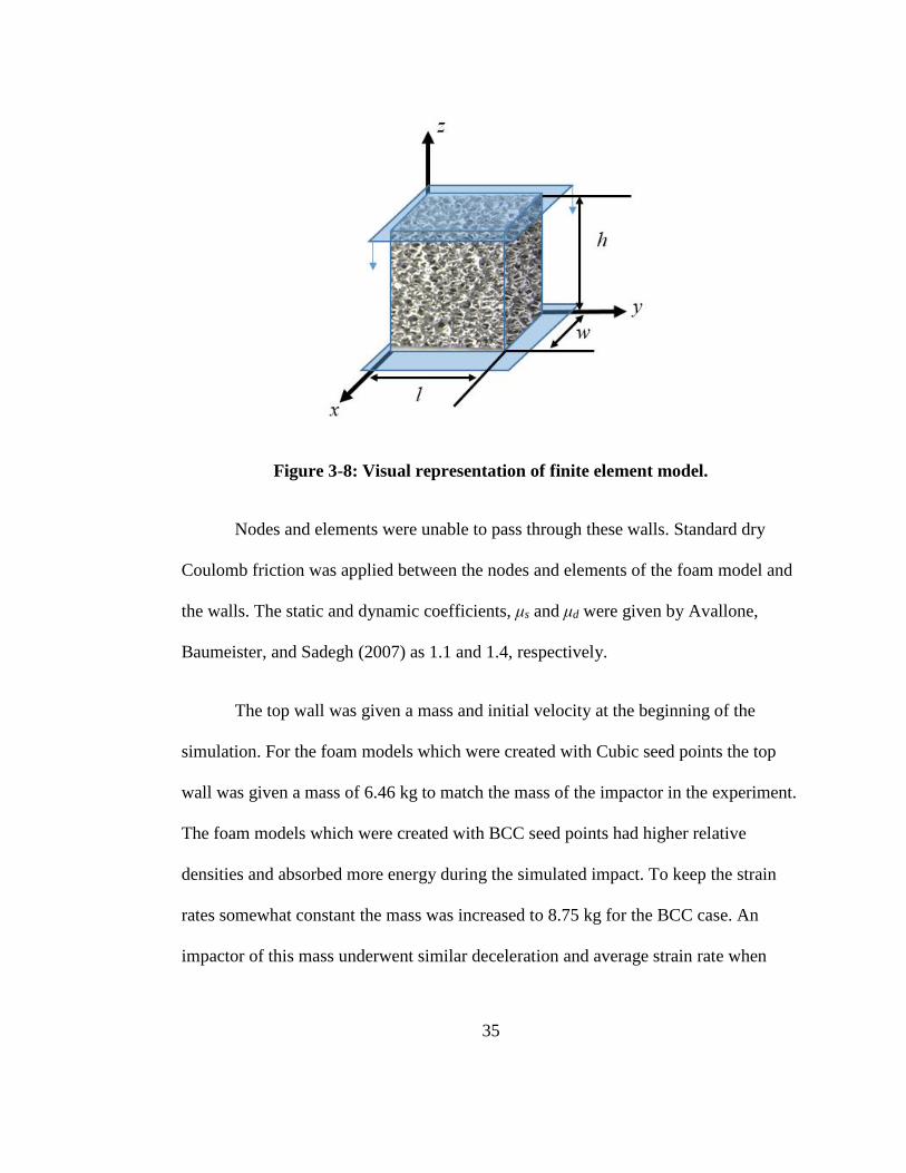
being the base material for Duocel foam. Boundary conditions for the foam were set

so that the nodes were unconstrained on all sides. Rigid walls were created on the top

and bottom of the foam cube as shown in blue in Figure 3-8.

35

Figure 3-8: Visual representation of finite element model.

Nodes and elements were unable to pass through these walls. Standard dry

Coulomb friction was applied between the nodes and elements of the foam model and

the walls. The static and dynamic coefficients, μs and μd were given by Avallone,

Baumeister, and Sadegh (2007) as 1.1 and 1.4, respectively.

The top wall was given a mass and initial velocity at the beginning of the

simulation. For the foam models which were created with Cubic seed points the top

wall was given a mass of 6.46 kg to match the mass of the impactor in the experiment.

The foam models which were created with BCC seed points had higher relative

densities and absorbed more energy during the simulated impact. To keep the strain

rates somewhat constant the mass was increased to 8.75 kg for the BCC case. An

impactor of this mass underwent similar deceleration and average strain rate when

36

impacting a BCC model as a 6.46 kg mass experienced when impacting a Cubic

model.

Force was measured across the top wall. Stress (given in Equation 1-4) was

computed by dividing this force by the initial area, lw. The foam model and real foams

undergo changes in cross-sectional area during large deformations. However, due to

the microstructure of the foam, this area change is not necessarily constant throughout

the z-direction of the foam. Finding the exact area for each of these slices would be

difficult to determine and it would vary from slice to slice. Further, most of the

literature referenced in Chapter 2, as well as ERG product literature report the stress

measure as engineering stress, rather than true stress. For these reasons, it was deemed

best to simply use the original area of the foam to calculate the stress.

Similarly, strain was reported as engineering strain (given in Equation 1-5).

The z displacement of the impacting wall was recorded and compared to the original

length of the sample. The equations below referencing the variables given in Figure 3-

8 were substituted in to Equations 1-4 and 1-5.

𝐴0 = 𝑙𝑤 (3-5)

ℎ = 𝐿0, 𝛥𝑧 = 𝛥ℎ = 𝛥𝐿 (3-6)

For each seed point method, several variations of the randomness parameter

were tested and compared. Additionally, a larger model was run which matched the

37

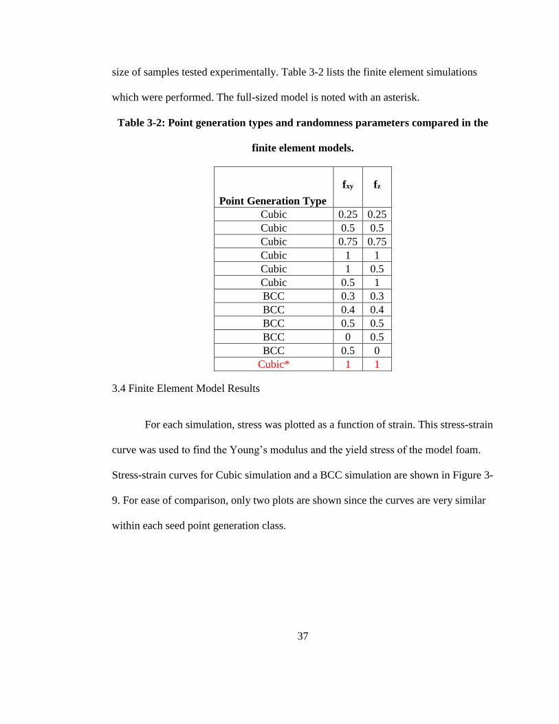
size of samples tested experimentally. Table 3-2 lists the finite element simulations

which were performed. The full-sized model is noted with an asterisk.

Table 3-2: Point generation types and randomness parameters compared in the

finite element models.

Point Generation Type

fxy fz

Cubic 0.25 0.25

Cubic 0.5 0.5

Cubic 0.75 0.75

Cubic 1 1

Cubic 1 0.5

Cubic 0.5 1

BCC 0.3 0.3

BCC 0.4 0.4

BCC 0.5 0.5

BCC 0 0.5

BCC 0.5 0

Cubic* 1 1

3.4 Finite Element Model Results

For each simulation, stress was plotted as a function of strain. This stress-strain

curve was used to find the Young’s modulus and the yield stress of the model foam.

Stress-strain curves for Cubic simulation and a BCC simulation are shown in Figure 3-

9. For ease of comparison, only two plots are shown since the curves are very similar

within each seed point generation class.

38

Figure 3-9: Representative stress-strain curves for simulations of two separate

seed point generation methods.

The Young’s modulus was found by calculating the slope, 𝛥𝜎

𝛥𝜀 , of the linear

portion of the curve (on the left side in Figure 3-9) using a linear regression fit. The

yield stress of the foam model was found by recording the stress at which the stress-

strain curve ceases to be linear. The curves for simulations of both cubic and BCC

seed point generation techniques had similar features: a steep, linear rise in stress

followed by a drop-off and subsequent plateau during which the models exhibited

plastic deformation. At between 60-70% strain, the curves rise in stress which

indicates densification. Tabulated data for each model is shown in Table 3-3.

0 10 20 30 40 50 60 70 80 90 1000

1

2

3

4

5

6

Strain (%)

Str

es

s (

MP

a)

Representative output: Stress as function of strain

Cubic: fx-.25 fy-.25 fz-.25

BCC: fx-.5 fy-.5 fz-.5

39

Table 3-3: Point generation types and randomness parameters compared in the

finite element model.

Point

Generation

Type fxy fz

Relative

Density

(%)

Number

of

Elements

Young's

Modulus

(Mpa)

Yield

Stress

(Mpa)

Cubic 0.25 0.25 7.47 11328 247 1.25

Cubic 0.5 0.5 7.04 11664 254 2.06

Cubic 0.75 0.75 6.45 11825 204 1.98

Cubic 1 1 5.91 12023 157 1.72

Cubic 1 0.5 6.70 11819 180 1.95

Cubic 0.5 1 7.00 11492 191 2.17

BCC 0.3 0.3 10.83 22657 533 5.06

BCC 0.4 0.4 10.93 22754 461 4.34

BCC 0.5 0.5 11.05 23054 375 3.94

BCC 0 0.5 10.55 21669 354 4.27

BCC 0.5 0 11.04 22995 617 4.66

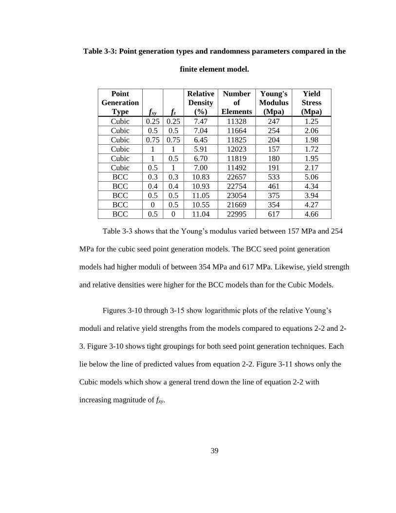
Table 3-3 shows that the Young’s modulus varied between 157 MPa and 254

MPa for the cubic seed point generation models. The BCC seed point generation

models had higher moduli of between 354 MPa and 617 MPa. Likewise, yield strength

and relative densities were higher for the BCC models than for the Cubic Models.

Figures 3-10 through 3-15 show logarithmic plots of the relative Young’s

moduli and relative yield strengths from the models compared to equations 2-2 and 2-

3. Figure 3-10 shows tight groupings for both seed point generation techniques. Each

lie below the line of predicted values from equation 2-2. Figure 3-11 shows only the

Cubic models which show a general trend down the line of equation 2-2 with

increasing magnitude of fxy.

40

Figure 3-10: Log-log plot of relative Young’s moduli for both seed point

generation methods compared with equation 2-2.

10-2

10-1

100

10-4

10-3

10-2

10-1

Relative Density f/

s

Rela

tive Y

ou

ng's

Mod

ulu

s E

f/Es

Relative Young's modulus as function of relative density

Cubic Seed Points

BCC Seed Points

𝐸𝑓

𝐸𝑠≈ (

𝜌𝑓

𝜌𝑠)2

41

Figure 3-11: Log-log plot of relative Young’s moduli for the cubic seed point

generation method compared with equation 2-2.

0.0398 0.0501 0.0631 0.0794 0.1

0.002

0.0025

0.0032

0.004

0.005

0.0063

0.0079

0.01

Relative Density f/

s

Rela

tiv

e Y

ou

ng

's M

od

ulu

s E

f/Es

Relative Young's modulus as function of relative density - Cubic




Cubic: fx-1 fy-1 fz-1

Cubic: fx-1 fy-1 fz-.5

Cubic: fx-.5 fy-.5 fz-1

𝐸𝑓

𝐸𝑠≈ (

𝜌𝑓

𝜌𝑠)2

42

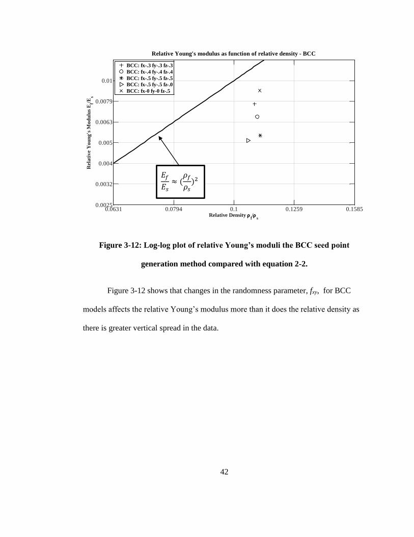
Figure 3-12: Log-log plot of relative Young’s moduli the BCC seed point


Figure 3-12 shows that changes in the randomness parameter, fxy, for BCC

models affects the relative Young’s modulus more than it does the relative density as

there is greater vertical spread in the data.

0.0631 0.0794 0.1 0.1259 0.15850.0025

0.0032

0.004

0.005

0.0063

0.0079

0.01

Relative Density f/

s

Rela

tiv

e Y

ou

ng

's M

od

ulu

s E

f/Es

Relative Young's modulus as function of relative density - BCC





BCC: fx-0 fy-0 fz-.5

𝐸𝑓

𝐸𝑠≈ (

𝜌𝑓

𝜌𝑠)2

43

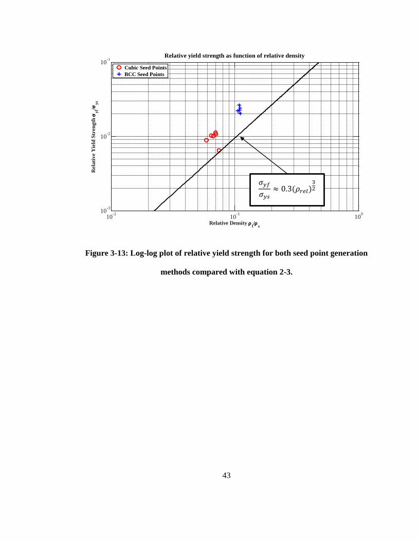
Figure 3-13: Log-log plot of relative yield strength for both seed point generation

methods compared with equation 2-3.

10-2

10-1

100

10-3

10-2

10-1

Relative Density f/

s

Rela

tive Y

ield

Str

en

gth

yf/

ys

Relative yield strength as function of relative density

Cubic Seed Points

BCC Seed Points

𝜎𝑦𝑓

𝜎𝑦𝑠≈ 0.3(𝜌𝑟𝑒𝑙)

32

44

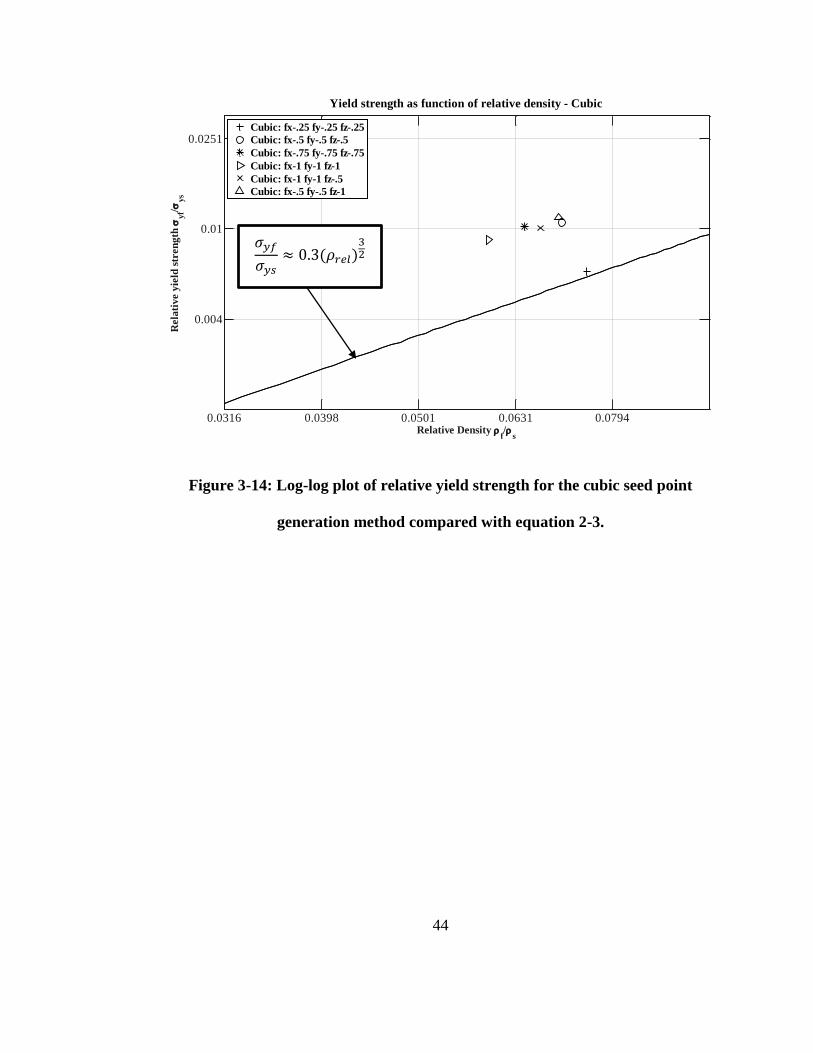
Figure 3-14: Log-log plot of relative yield strength for the cubic seed point


0.0316 0.0398 0.0501 0.0631 0.0794

0.004

0.01

0.0251

Relative Density f/

s

Rela

tiv

e y

ield

str

en

gth

yf/

ys

Yield strength as function of relative density - Cubic




Cubic: fx-1 fy-1 fz-1

Cubic: fx-1 fy-1 fz-.5

Cubic: fx-.5 fy-.5 fz-1

𝜎𝑦𝑓


32

45

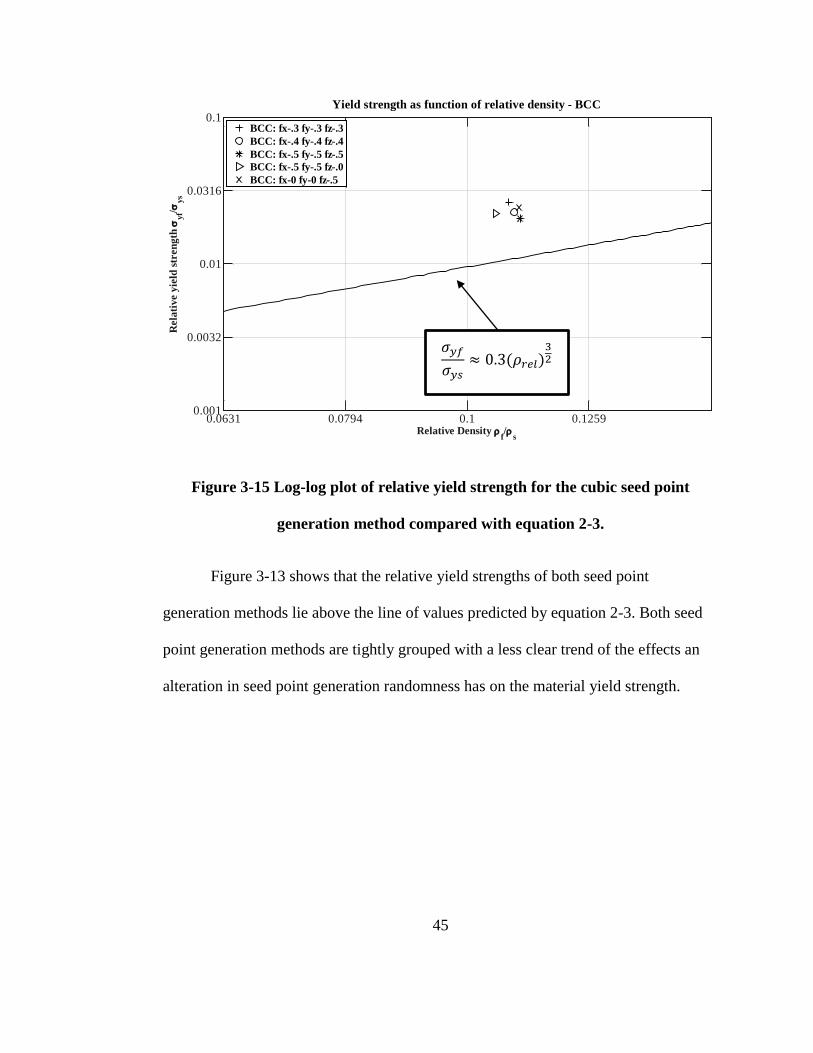
Figure 3-15 Log-log plot of relative yield strength for the cubic seed point


Figure 3-13 shows that the relative yield strengths of both seed point

generation methods lie above the line of values predicted by equation 2-3. Both seed

point generation methods are tightly grouped with a less clear trend of the effects an

alteration in seed point generation randomness has on the material yield strength.

0.0631 0.0794 0.1 0.12590.001

0.0032

0.01

0.0316

0.1

Relative Density f/

s

Rela

tiv

e y

ield

str

en

gth

yf/

ys

Yield strength as function of relative density - BCC





BCC: fx-0 fy-0 fz-.5

𝜎𝑦𝑓


32

46

CHAPTER 4

COMPRESSION EXPERIMENTS

4.1 Introduction

Drop weight experiments were performed on open-cell metal foam samples in

order to compare their results with those of the finite element modeling. Samples of

varying porosities were subjected to loading at a strain rate of 110/s. High speed

photography was used to view the samples as they were compressed. The high speed

photography was used to visualize crush patterns within the samples and interpret the

results.

4.2 Experimental Method

Samples of Duocel open-cell aluminum foam of porosity 10 PPI, 20 PPI, and

40 PPI were purchased from KRReynolds Company, which is a distributor of ERG

Duocel foam materials. All samples were listed to have 8% nominal relative density

and were made of 6101-T6 Aluminum base material. Each sample was then weighed

and measured in order to obtain the true relative density. The measured relative

densities are given in Table 4-1. The densities for both 10PPI and 20PPI foams were

close to the manufacturer’s specification, but the 40PPI foam diverged by ~1.2%.

47

Table 4-1: Name, porosity, and relative density of each compression experiment

sample.

Sample

Name

Porosity

(PPI)

Relative

Density (%)

10 PPI - 1 10 7.95

10 PPI - 2 10 7.95

20 PPI - 1 20 7.82

20 PPI - 2 20 7.82

40 PPI - 1 40 6.40

40 PPI - 2 40 6.40

The samples were originally 3.5” long by 1.5” wide x .5” thick, but were cut by hand

with a band saw to 1.75” long, by 1.5” wide x .5” thick. Although careful attention

was paid to maintain square edges, it was noted that after cutting some edges of some

samples were slightly skewed. Attempts were made to get samples which were

thicker, however .5” was the thickest size available.

After the samples were cut, the 1.5” x 1.75” face of each sample which would

be facing the high-speed camera was painted with black Por 15 priming paint. Por 15

was chosen due to its rugged adherence to a range of different metals. The paint was

carefully dabbed on to the front ligaments of the sample. Outward-facing ligaments

down to approximately one cell’s width beneath the surface were covered across the

entire surface. It was hoped that the black color would add contrast to the cellular

ligaments to assist in visualizing crush zone formation and cellular deformation.

The samples were then placed in an Instron Dynatup 9210 dynamic testing

machine and aligned with the center of the impactor. The impactor was a 2” diameter

48

by 2” long steel bar which was attached to the machine by a threaded bolt. The surface

of the impactor which would contact the sample was machined smooth in a lathe and

then sanded with a fine-grit sand paper.

A Photron SA1 high-speed camera was then focused on the front face of the

sample with an f8 aperture setting which balanced lighting conditions with depth of

field. High-power lighting was focused on the sample. It should be noted that due to

the intensity of the light, considerable temperature rise was observed in the sample.

Although warm to the touch, the sample was still able to be held.

The impactor was raised and then dropped at free-fall in order to crush the

samples. Raising the impactor to its greatest height yielded an impact velocity of 4.86

meters per second which is a strain rate of ~109/s. The mass of the impactor and frame

together was 6.36 kilograms. As the impactor made contact with the sample, a load

cell was used to measure the force on the impactor as a function of time. Velocity at

the time of impact was also measured by the machine. Concurrently, the camera was

triggered to take pictures at 10,000 frames per second. These pictures were then

compiled into a video.

The Dynatup machine outputs a force signal from its load cell. This force

signal is scaled by a ratio of the total mass impacting the specimen to the mass of the

crosshead. The scaled result is the force “seen” by the sample during the impact event.

The scaled force is then divided by the total mass in order to get acceleration. The

acceleration is numerically integrated to get the velocity. The velocity is then

49

numerically integrated to get the displacement of the impactor as it hits the sample.

Both integrations are trapezoidal and the acceleration due to gravity during sample

deformation is neglected. The final displacement is used to get the strain.

MATLAB image analysis was used to turn the video from grayscale to binary

(enhancing contrast). The threshold of .25 was chosen because it seemed to give the

best view of the ligaments.

4.3 Experiment Results and Data Processing

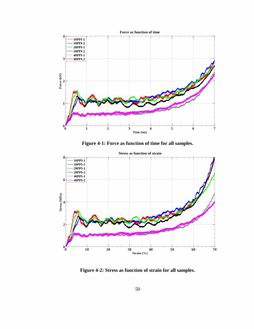
Figures 4-1 and 4-2 show the force-time curves and stress-strain curves

obtained from the samples tested in the experiments. Both 10PPI and 20PPI samples

have similarly shaped curves which have steep rises on the left-hand side followed by

a plateau and a final rise as sample densification occurs.

The stress-strain curves were then used to compute both the Young’s modulus

and yield stress of the samples. The modulus of each sample was originally computed

using a linear regression fit of the first 250 points of the stress-strain curve, which was

assumed to be linear. The values obtained in this approach are listed in the second

column, “Young’s 1”, of Table 4-2.

50

Figure 4-1: Force as function of time for all samples.

Figure 4-2: Stress as function of strain for all samples.

0 1 2 3 4 5 6 70

1

2

3

4Force as function of time

Time (ms)

Force (

kN

)

10PPI-1

10PPI-2

20PPI-1

20PPI-2

40PPI-1

40PPI-2

0 10 20 30 40 50 60 700

2

4

6

8Stress as function of strain

Strain (%)

Str

ess

(M

Pa)

10PPI-1

10PPI-2

20PPI-1

20PPI-2

40PPI-1

40PPI-2

51

Duocel foam is listed as having a compressive modulus of 100 MPa and yield

strength 2.53 MPa. As seen from the table, the originally computed values are notably

lower than these manufacturer’s specifications. Comparison between the stress-strain

data curves and the high speed camera footage reveals that due to the slightly-skewed

edges of some of the samples the impactor makes contact with only an edge before the

sample “seats” to have both top and bottom faces parallel with the impactor. This

process takes about 2 frames or .2 ms. This .2 ms seating process aligns well with

visible nonlinearities, or “kinks” in the initial portions of the force-time and stress-

strain curves.

Due to this observation, the Young’s modulus was recomputed using the linear

portion of the stress-strain curve directly after the kinks (see column “Youngs 2” in

Table 4-2). The recomputed Young’s values matched well with expected values.

Figure 4-3 shows the force-time curve of sample 10PPI-1 with the aforementioned

kink. The portion used to get the Young’s modulus is noted in red. On the right side of

Figure 4-3 is a plot of the rise in the stress-strain curve. The linear regression fits (with

zero intercept) of the first 250 points and of the red section of the force-time curve are

shown in red and green, respectively. It is evident from the right-hand plot that the

green line, “Linear Int. 2” matches the slope of the stress-strain after the kink. This

slope adjustment is carried out for the remaining samples. Adjusted values are listed in

the third column of Table 4-2.

52

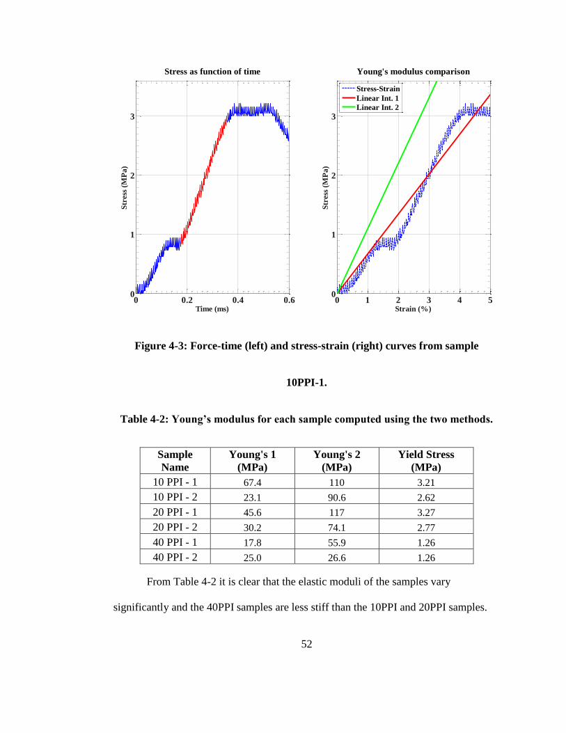
Figure 4-3: Force-time (left) and stress-strain (right) curves from sample

10PPI-1.

Table 4-2: Young’s modulus for each sample computed using the two methods.

Sample

Name

Young's 1

(MPa)

Young's 2

(MPa)

Yield Stress

(MPa)

10 PPI - 1 67.4 110 3.21

10 PPI - 2 23.1 90.6 2.62

20 PPI - 1 45.6 117 3.27

20 PPI - 2 30.2 74.1 2.77

40 PPI - 1 17.8 55.9 1.26

40 PPI - 2 25.0 26.6 1.26

From Table 4-2 it is clear that the elastic moduli of the samples vary

significantly and the 40PPI samples are less stiff than the 10PPI and 20PPI samples.

0 1 2 3 4 50

1

2

3

Young's modulus comparison

Strain (%)

Str

ess

(M

Pa

)

Stress-Strain

Linear Int. 1

Linear Int. 2

0 0.2 0.4 0.60

1

2

3

Stress as function of time

Time (ms)

Str

ess

(M

Pa

)

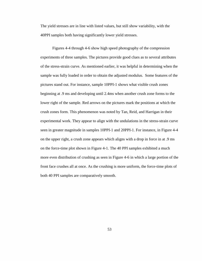
53

The yield stresses are in line with listed values, but still show variability, with the

40PPI samples both having significantly lower yield stresses.

Figures 4-4 through 4-6 show high speed photography of the compression

experiments of three samples. The pictures provide good clues as to several attributes

of the stress-strain curve. As mentioned earlier, it was helpful in determining when the

sample was fully loaded in order to obtain the adjusted modulus. Some features of the

pictures stand out. For instance, sample 10PPI-1 shows what visible crush zones

beginning at .9 ms and developing until 2.4ms when another crush zone forms to the

lower right of the sample. Red arrows on the pictures mark the positions at which the

crush zones form. This phenomenon was noted by Tan, Reid, and Harrigan in their

experimental work. They appear to align with the undulations in the stress-strain curve

seen in greater magnitude in samples 10PPI-1 and 20PPI-1. For instance, in Figure 4-4

on the upper right, a crush zone appears which aligns with a drop in force in at .9 ms

on the force-time plot shown in Figure 4-1. The 40 PPI samples exhibited a much

more even distribution of crushing as seen in Figure 4-6 in which a large portion of the

front face crushes all at once. As the crushing is more uniform, the force-time plots of

both 40 PPI samples are comparatively smooth.

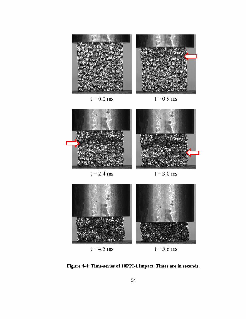
54

Figure 4-4: Time-series of 10PPI-1 impact. Times are in seconds.

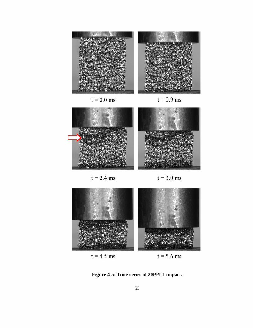
55

Figure 4-5: Time-series of 20PPI-1 impact.

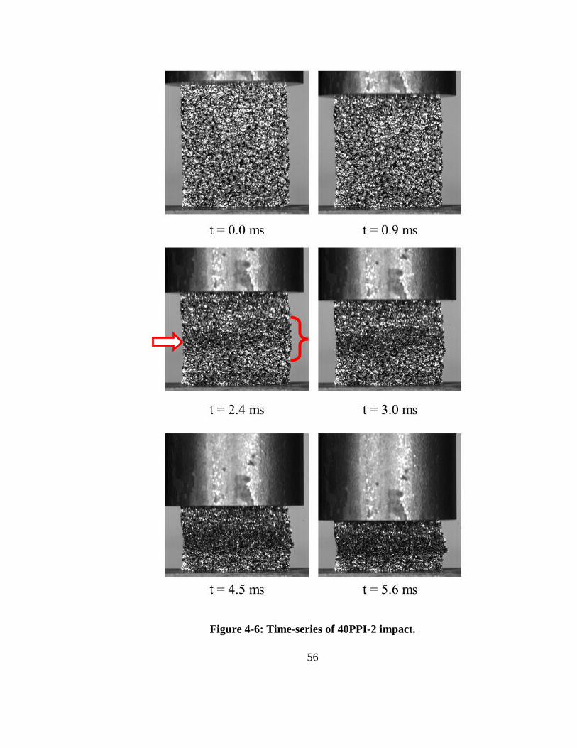
56

Figure 4-6: Time-series of 40PPI-2 impact.

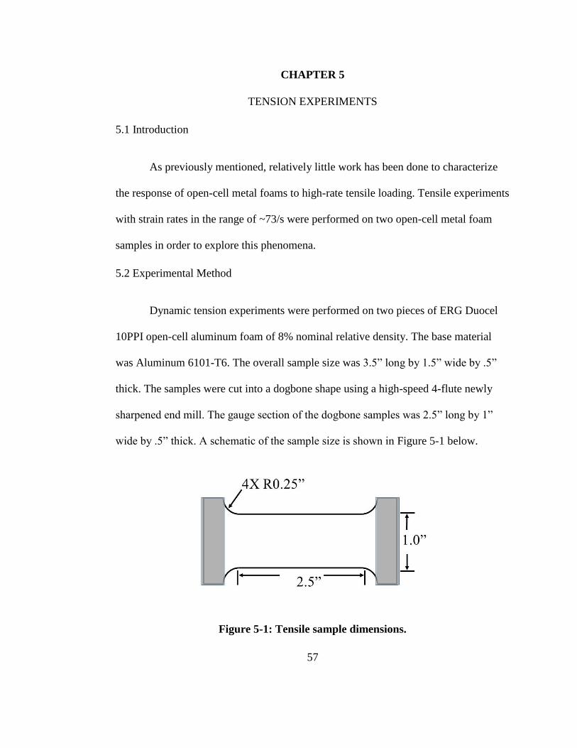
57

CHAPTER 5

TENSION EXPERIMENTS

5.1 Introduction

As previously mentioned, relatively little work has been done to characterize

the response of open-cell metal foams to high-rate tensile loading. Tensile experiments

with strain rates in the range of ~73/s were performed on two open-cell metal foam

samples in order to explore this phenomena.

5.2 Experimental Method

Dynamic tension experiments were performed on two pieces of ERG Duocel

10PPI open-cell aluminum foam of 8% nominal relative density. The base material

was Aluminum 6101-T6. The overall sample size was 3.5” long by 1.5” wide by .5”

thick. The samples were cut into a dogbone shape using a high-speed 4-flute newly

sharpened end mill. The gauge section of the dogbone samples was 2.5” long by 1”

wide by .5” thick. A schematic of the sample size is shown in Figure 5-1 below.

Figure 5-1: Tensile sample dimensions.

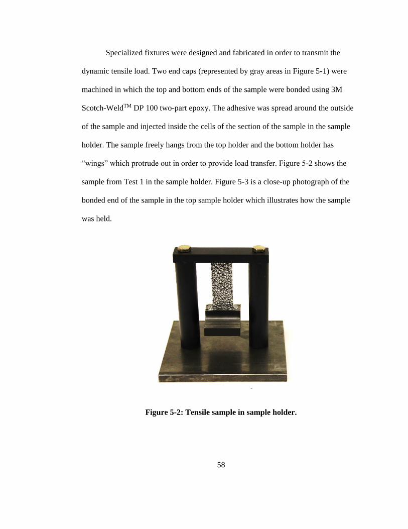
58

Specialized fixtures were designed and fabricated in order to transmit the

dynamic tensile load. Two end caps (represented by gray areas in Figure 5-1) were

machined in which the top and bottom ends of the sample were bonded using 3M

Scotch-WeldTM DP 100 two-part epoxy. The adhesive was spread around the outside

of the sample and injected inside the cells of the section of the sample in the sample

holder. The sample freely hangs from the top holder and the bottom holder has

“wings” which protrude out in order to provide load transfer. Figure 5-2 shows the

sample from Test 1 in the sample holder. Figure 5-3 is a close-up photograph of the

bonded end of the sample in the top sample holder which illustrates how the sample

was held.

Figure 5-2: Tensile sample in sample holder.

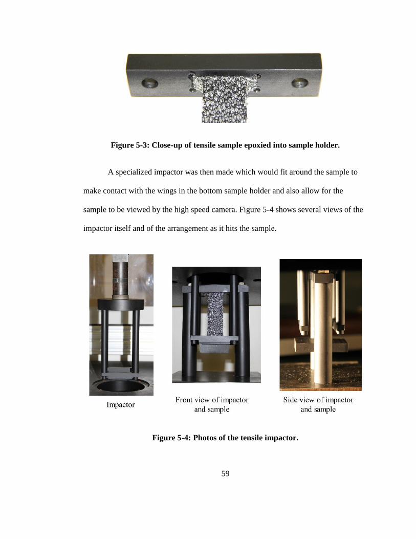
59

Figure 5-3: Close-up of tensile sample epoxied into sample holder.

A specialized impactor was then made which would fit around the sample to

make contact with the wings in the bottom sample holder and also allow for the

sample to be viewed by the high speed camera. Figure 5-4 shows several views of the

impactor itself and of the arrangement as it hits the sample.

Figure 5-4: Photos of the tensile impactor.

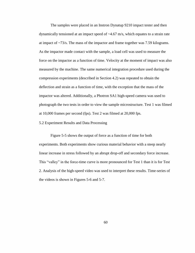
60

The samples were placed in an Instron Dynatup 9210 impact tester and then

dynamically tensioned at an impact speed of ~4.67 m/s, which equates to a strain rate

at impact of ~73/s. The mass of the impactor and frame together was 7.59 kilograms.

As the impactor made contact with the sample, a load cell was used to measure the

force on the impactor as a function of time. Velocity at the moment of impact was also

measured by the machine. The same numerical integration procedure used during the

compression experiments (described in Section 4.2) was repeated to obtain the

deflection and strain as a function of time, with the exception that the mass of the

impactor was altered. Additionally, a Photron SA1 high-speed camera was used to

photograph the two tests in order to view the sample microstructure. Test 1 was filmed

at 10,000 frames per second (fps). Test 2 was filmed at 20,000 fps.

5.2 Experiment Results and Data Processing

Figure 5-5 shows the output of force as a function of time for both

experiments. Both experiments show curious material behavior with a steep nearly

linear increase in stress followed by an abrupt drop-off and secondary force increase.

This “valley” in the force-time curve is more pronounced for Test 1 than it is for Test

2. Analysis of the high-speed video was used to interpret these results. Time-series of

the videos is shown in Figures 5-6 and 5-7.

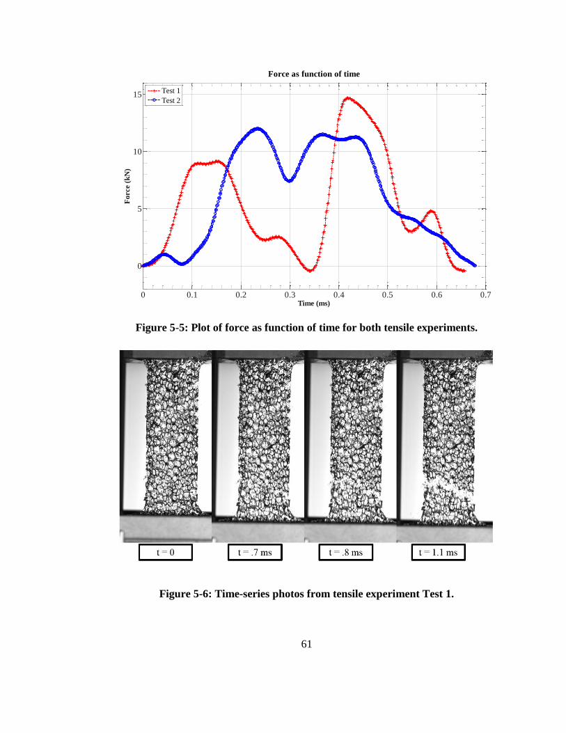
61

Figure 5-5: Plot of force as function of time for both tensile experiments.

Figure 5-6: Time-series photos from tensile experiment Test 1.

0 0.1 0.2 0.3 0.4 0.5 0.6 0.7

0

5

10

15

Force as function of time

Time (ms)

Fo

rce (

kN

)

Test 1

Test 2

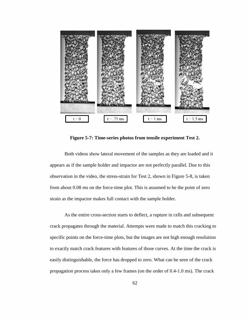
62

Figure 5-7: Time-series photos from tensile experiment Test 2.

Both videos show lateral movement of the samples as they are loaded and it

appears as if the sample holder and impactor are not perfectly parallel. Due to this

observation in the video, the stress-strain for Test 2, shown in Figure 5-8, is taken

from about 0.08 ms on the force-time plot. This is assumed to be the point of zero

strain as the impactor makes full contact with the sample holder.

As the entire cross-section starts to deflect, a rupture in cells and subsequent

crack propagates through the material. Attempts were made to match this cracking to

specific points on the force-time plots, but the images are not high enough resolution

to exactly match crack features with features of those curves. At the time the crack is

easily distinguishable, the force has dropped to zero. What can be seen of the crack

propagation process takes only a few frames (on the order of 0.4-1.0 ms). The crack

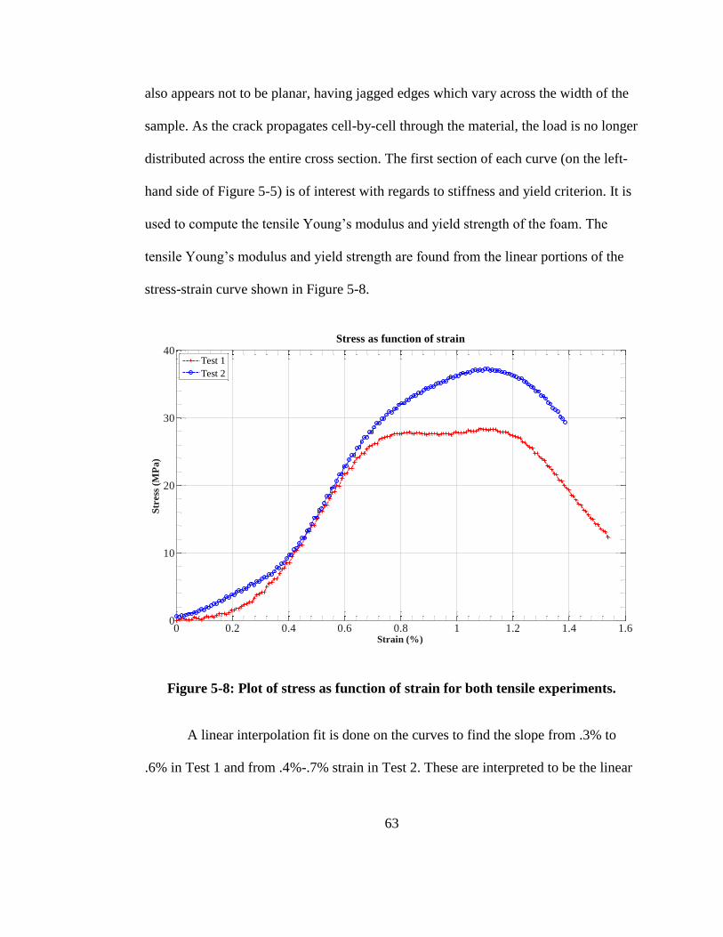
63

also appears not to be planar, having jagged edges which vary across the width of the

sample. As the crack propagates cell-by-cell through the material, the load is no longer

distributed across the entire cross section. The first section of each curve (on the left-

hand side of Figure 5-5) is of interest with regards to stiffness and yield criterion. It is

used to compute the tensile Young’s modulus and yield strength of the foam. The

tensile Young’s modulus and yield strength are found from the linear portions of the

stress-strain curve shown in Figure 5-8.

Figure 5-8: Plot of stress as function of strain for both tensile experiments.

A linear interpolation fit is done on the curves to find the slope from .3% to

.6% in Test 1 and from .4%-.7% strain in Test 2. These are interpreted to be the linear

0 0.2 0.4 0.6 0.8 1 1.2 1.4 1.60

10

20

30


Strain (%)

Str

ess

(M

Pa

)

Test 1

Test 2

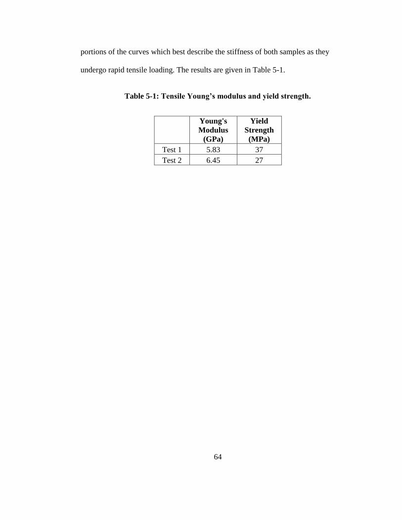
64

portions of the curves which best describe the stiffness of both samples as they

undergo rapid tensile loading. The results are given in Table 5-1.

Table 5-1: Tensile Young’s modulus and yield strength.

Young's

Modulus

(GPa)

Yield

Strength

(MPa)

Test 1 5.83 37

Test 2 6.45 27

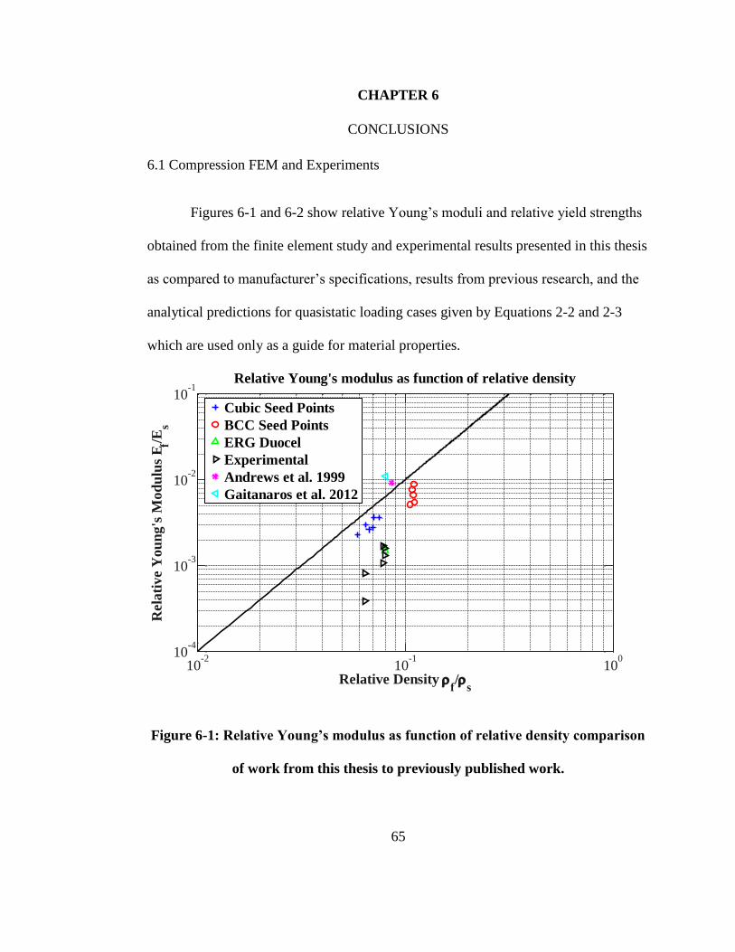
65

CHAPTER 6

CONCLUSIONS

6.1 Compression FEM and Experiments

Figures 6-1 and 6-2 show relative Young’s moduli and relative yield strengths

obtained from the finite element study and experimental results presented in this thesis

as compared to manufacturer’s specifications, results from previous research, and the

analytical predictions for quasistatic loading cases given by Equations 2-2 and 2-3

which are used only as a guide for material properties.

Figure 6-1: Relative Young’s modulus as function of relative density comparison

of work from this thesis to previously published work.

10-2

10-1

100

10-4

10-3

10-2

10-1

Relative Density f/

s

Rela

tiv

e Y

ou

ng

's M

od

ulu

s E

f/Es

Relative Young's modulus as function of relative density

Cubic Seed Points

BCC Seed Points

ERG Duocel

Experimental

Andrews et al. 1999

Gaitanaros et al. 2012

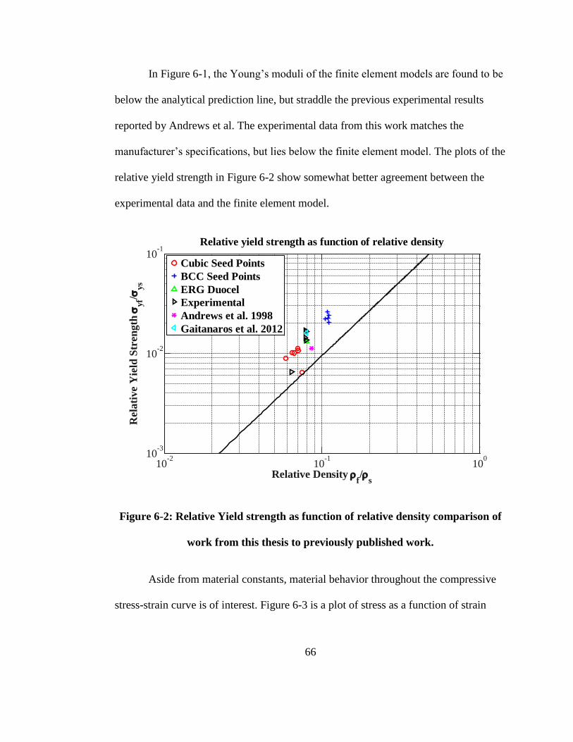
66

In Figure 6-1, the Young’s moduli of the finite element models are found to be

below the analytical prediction line, but straddle the previous experimental results

reported by Andrews et al. The experimental data from this work matches the

manufacturer’s specifications, but lies below the finite element model. The plots of the

relative yield strength in Figure 6-2 show somewhat better agreement between the

experimental data and the finite element model.

Figure 6-2: Relative Yield strength as function of relative density comparison of

work from this thesis to previously published work.

Aside from material constants, material behavior throughout the compressive

stress-strain curve is of interest. Figure 6-3 is a plot of stress as a function of strain

10-2

10-1

100

10-3

10-2

10-1

Relative Density f/

s

Rela

tive Y

ield

Str

en

gth

yf/

ys

Relative yield strength as function of relative density

Cubic Seed Points

BCC Seed Points

ERG Duocel

Experimental

Andrews et al. 1998

Gaitanaros et al. 2012

67

from the models created by Gaitanaros, Kyriakides, and Kraynik (2012). The stress-

strain data produced from both models and experiments from the present work is

shown in Figure 6-4.

Figure 6-3: Stress-strain curve from Gaitanaros, Kyriakides, and Kraynik (2012)

Figure 6-4: Stress-strain curves from experimental and FEM data

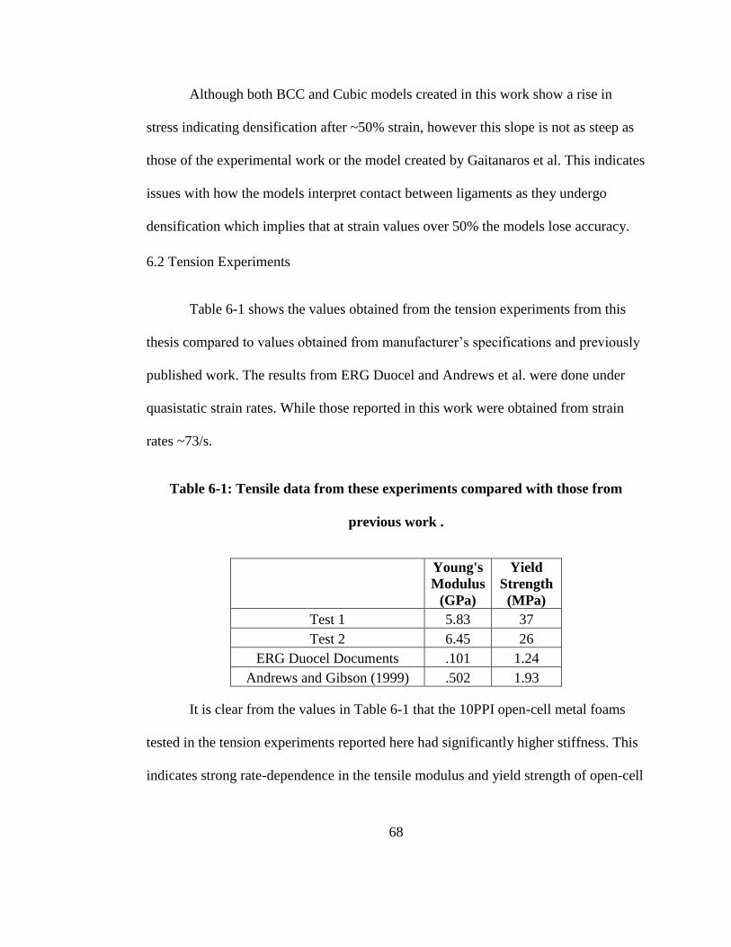
68

Although both BCC and Cubic models created in this work show a rise in

stress indicating densification after ~50% strain, however this slope is not as steep as

those of the experimental work or the model created by Gaitanaros et al. This indicates

issues with how the models interpret contact between ligaments as they undergo

densification which implies that at strain values over 50% the models lose accuracy.

6.2 Tension Experiments

Table 6-1 shows the values obtained from the tension experiments from this

thesis compared to values obtained from manufacturer’s specifications and previously

published work. The results from ERG Duocel and Andrews et al. were done under

quasistatic strain rates. While those reported in this work were obtained from strain

rates ~73/s.

Table 6-1: Tensile data from these experiments compared with those from

previous work .

Young's

Modulus

(GPa)

Yield

Strength

(MPa)

Test 1 5.83 37

Test 2 6.45 26

ERG Duocel Documents .101 1.24

Andrews and Gibson (1999) .502 1.93

It is clear from the values in Table 6-1 that the 10PPI open-cell metal foams

tested in the tension experiments reported here had significantly higher stiffness. This

indicates strong rate-dependence in the tensile modulus and yield strength of open-cell

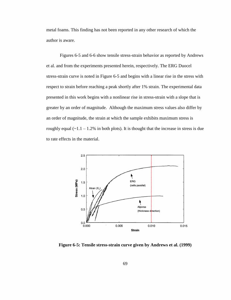
69

metal foams. This finding has not been reported in any other research of which the

author is aware.

Figures 6-5 and 6-6 show tensile stress-strain behavior as reported by Andrews

et al. and from the experiments presented herein, respectively. The ERG Duocel

stress-strain curve is noted in Figure 6-5 and begins with a linear rise in the stress with

respect to strain before reaching a peak shortly after 1% strain. The experimental data

presented in this work begins with a nonlinear rise in stress-strain with a slope that is

greater by an order of magnitude. Although the maximum stress values also differ by

an order of magnitude, the strain at which the sample exhibits maximum stress is

roughly equal (~1.1 – 1.2% in both plots). It is thought that the increase in stress is due

to rate effects in the material.

Figure 6-5: Tensile stress-strain curve given by Andrews et al. (1999)

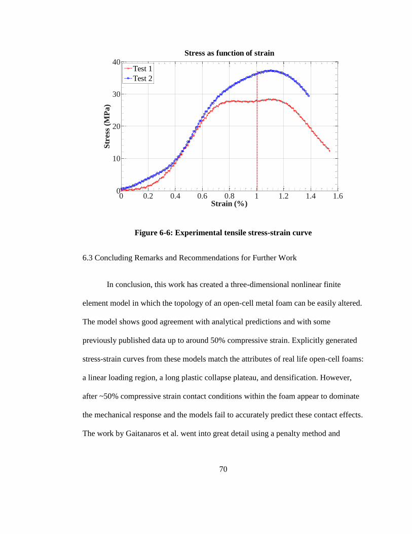
70

Figure 6-6: Experimental tensile stress-strain curve

6.3 Concluding Remarks and Recommendations for Further Work

In conclusion, this work has created a three-dimensional nonlinear finite

element model in which the topology of an open-cell metal foam can be easily altered.

The model shows good agreement with analytical predictions and with some

previously published data up to around 50% compressive strain. Explicitly generated

stress-strain curves from these models match the attributes of real life open-cell foams:

a linear loading region, a long plastic collapse plateau, and densification. However,

after ~50% compressive strain contact conditions within the foam appear to dominate

the mechanical response and the models fail to accurately predict these contact effects.

The work by Gaitanaros et al. went into great detail using a penalty method and

0 0.2 0.4 0.6 0.8 1 1.2 1.4 1.60

10

20

30


Strain (%)

Str

ess

(M

Pa

)

Test 1

Test 2

71

defining an interface stiffness between ligaments. This work used a simpler method

which decreased computation time, but limited accuracy at high strains. Better

estimates of friction coefficients or erosion parameters within the material could be

used to increase accuracy. Mechanical constants taken from below the 50%

compressive strain value are deemed to be reliable indicators of foam behavior.

Two seed point generation techniques for a three dimensional Voronoi lattice

were explored and used to look at the effects of seed point positional perturbations on

the elastic-plastic response of the foam. While more work is needed to make firmer

conclusions, several can be made from the data presented herein.

First, a BCC seed point generation technique will create foams with higher

relative moduli than a cubic seed point generation technique. Second, increasing

perturbations in the seed point position will decrease the relative stiffness of the foam.

These results agree with the conclusions made by Alkhader and Vural (2008) who

made this same conclusion about the loss of periodicity in 2D foams. Finally, the

mechanical properties of foams created with BCC seed points have greater sensitivity

to seed point perturbations than do their relative densities. The last point is important

because it shows that in a BCC foam, alterations in the seed point perturbations can

change the mechanical characteristics of the foam without a comparative increase in

the relative density of the foam. As the relative density is related to weight and cost,

this finding can be used to tailor foams for specific applications.

72

Results from the compression experiments performed in this work are deemed

to be less reliable as there were imperfections in material preparation which affected

the results. In addition, the thin sample size available off the shelf produced out-of-

plane bending and buckling which may have impacted the results. Still, crush patterns

were clearly visible in the high speed photography and the experiments were valuable

to compare to finite element models of the same size. These crush patterns were more

visible in the lower porosity samples than the higher ones.

The tensile tests produced results which show evidence of strain-rate hardening

in open-cell metal foams. While the low compressive plastic yield stress and longer

strain plateau of these foams make them suitable energy absorbers, the significantly

higher stiffness attributed to dynamic tensile loading indicates that these materials

make poor tensile energy absorbers.

The models created in this work were helpful in comparing material stiffness

and yield strength of open-cell metal foams, but their usefulness could also be

extended to energy absorption of the foams. This work was limited in computing

power, but larger models with more elements per strut could easily be studied. Further,

functional gradation of the material is possible by altering the seed point locations or

strut diameters throughout. In an effort to improve the modeling beyond 50% strain

and into densification much more work could be done in understanding the

complicated contact conditions within the foam. Varying friction between struts

during the crush plateau would provide interesting insight and targeted studies on

73

specific contact scenarios would help further define contact conditions. These models

are adaptable and have already shown use in understanding foam material properties,

but also provide the foundation for further research.

74

APPENDIX A

MATLAB SOFTWARE TO CREATE SEED POINTS, NODES, AND ELEMENTS

%--------------------------------------- % K_FILE_CREATE clear all;close all; clc % % Created by Colin J. Murphy % % Description: K_FILE_CREATE is script which runs the object-oriented % routines Element and Node. These routines read file output from

%Voro++ % 3D voronoi cell library and % then create "nod_list.k" and "el_list.k" and node and element files

%in % LS-DYNA keyword format. % To use, one would use "random_point_gen.m" to % output a list of seed points. This list is put into Voro++ using

%the % "import" function found here:

http://math.lbl.gov/voro++/examples/import/ % following the pack_ten_cube example. Voro++ is a C++ library which

%can % easily be compiled in linux. % % Make sure to change the file names and max/min values in the

%"import" % file to match the ones created in random_point_gen. Use the file

ouput % from import (in the example, it is "pack_ten_cube.gnu") as "fname"

in the % script below % % First, GNU_V_reader parses the file to determine the cells and node % locations. Node.m uses that information to create the node list and % Element.m uses the Node information to create the element list. %--------------------------------------- % Options % % directory -> the directory in which Voro++ output file is placed

and % where element % % sf -> scale factor to scale the model from "cells" to meters % % fname -> Voro++ output file with voronoi cell locations % % directory = 'C:’; fname = 'Cube_10x10x10_fx-1_fy-1_fz-1_1.gnu'; sf = .0033;

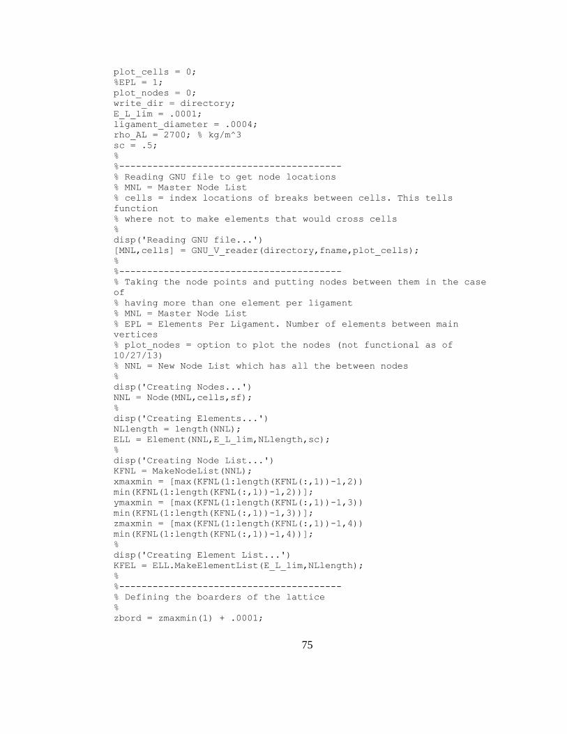
75

plot_cells = 0; %EPL = 1; plot_nodes = 0; write_dir = directory; E_L_lim = .0001; ligament_diameter = .0004; rho_AL = 2700; % kg/m^3 sc = .5; % %---------------------------------------- % Reading GNU file to get node locations % MNL = Master Node List % cells = index locations of breaks between cells. This tells

function % where not to make elements that would cross cells % disp('Reading GNU file...') [MNL,cells] = GNU_V_reader(directory,fname,plot_cells); % %---------------------------------------- % Taking the node points and putting nodes between them in the case

of % having more than one element per ligament % MNL = Master Node List % EPL = Elements Per Ligament. Number of elements between main

vertices % plot_nodes = option to plot the nodes (not functional as of

10/27/13) % NNL = New Node List which has all the between nodes % disp('Creating Nodes...') NNL = Node(MNL,cells,sf); % disp('Creating Elements...') NLlength = length(NNL); ELL = Element(NNL,E_L_lim,NLlength,sc); % disp('Creating Node List...') KFNL = MakeNodeList(NNL); xmaxmin = [max(KFNL(1:length(KFNL(:,1))-1,2))

min(KFNL(1:length(KFNL(:,1))-1,2))]; ymaxmin = [max(KFNL(1:length(KFNL(:,1))-1,3))

min(KFNL(1:length(KFNL(:,1))-1,3))]; zmaxmin = [max(KFNL(1:length(KFNL(:,1))-1,4))

min(KFNL(1:length(KFNL(:,1))-1,4))]; % disp('Creating Element List...') KFEL = ELL.MakeElementList(E_L_lim,NLlength); % %---------------------------------------- % Defining the boarders of the lattice % zbord = zmaxmin(1) + .0001;

76

xbord1 = xmaxmin(1); xbord2 = xmaxmin(2); ybord1 = ymaxmin(1); ybord2 = ymaxmin(2); % % shell_nodes are used for the rigidwalls which impact the Lattice % shell_nodes = [199999,xbord2,ybord2,zbord,0,0;... 199998,xbord2,ybord1,zbord,0,0;... 199997,xbord1,ybord1,zbord,0,0;... 199996,xbord1,ybord2,zbord,0,0]; % Element_Lengths = ELL.Compute_Lengths(E_L_lim); Area = xmaxmin(1)*ymaxmin(1); Length = zmaxmin(1); Volume = xmaxmin(1)*ymaxmin(1)*zmaxmin(1); Surface_Area = sum(Element_Lengths)*pi*ligament_diameter; Relative_Density =

((sum(Element_Lengths)*(pi*((ligament_diameter^2))/4)... *rho_AL)/(rho_AL*Volume))*100; % %---------------------------------------- % Writing 3 files: % % nod_list.k is the list of nodes used in the LS-DYNA simulations.

The % nodes are then used in the element list. The last four nodes are

used to % define the rigidwall which impacts the sample % % el_list.k is the list of elements created from the node list % % run_stats.txt has the size of the sample, relative density

computation, % and volume. It also has a list of the length of every element in

the % computation if length statistics are desired %

cd(write_dir);

disp('Writing Node File...')

fid = fopen('nod_list.k','w'); fprintf(fid,'%s\r\n','*keyword'); fprintf(fid,'%s\r\n','*NODE'); fclose(fid); dlmwrite('nod_list.k',KFNL,'-

append','roffset',0,'newline','pc','precision',6); dlmwrite('nod_list.k',shell_nodes,'-

append','roffset',0,'newline','pc','precision',6);

77

disp('Writing Element File...')

fid = fopen('el_list.k','w'); fprintf(fid,'%s\r\n','*keyword'); fprintf(fid,'%s\r\n','*ELEMENT_BEAM'); fclose(fid); dlmwrite('el_list.k',KFEL,'-

append','roffset',0,'newline','pc','precision',6);

disp('Writing Stats File...')

fid = fopen('run_stats.txt','w'); fprintf(fid,'%s\r\n',(['Element Limit: ',num2str(E_L_lim)])); fprintf(fid,'%s\r\n',(['Scale Factor: ',num2str(sf)])); fprintf(fid,'%s\r\n',(['Area: ',num2str(Area)])); fprintf(fid,'%s\r\n',(['Ligament Diameter:

',num2str(ligament_diameter)])); fprintf(fid,'%s\r\n',(['Height: ',num2str(Length)])); fprintf(fid,'%s\r\n',(['Volume: ',num2str(Volume)])); fprintf(fid,'%s\r\n',(['Surface Area: ',num2str(Surface_Area)])); fprintf(fid,'%s\r\n',(['Relative Density:

',num2str(Relative_Density)])); fclose(fid); dlmwrite('run_stats.txt',Element_Lengths,'-

append','roffset',0,'newline','pc')

---------------------------------

function[MNL,cells] = GNU_V_reader(directory,fname,plot_cells)

% When in standalone mode, uncomment the lines below % clear all % clc % cd('C:\Users\Colin\Desktop\MATLAB NODE MAKER'); % fname = 'random_points_v.txt'; % fname = 'pack_six_cube.txt'; %% Change in to datafile directory cd(directory); % Opening file and reading in data fid = fopen(fname); % Taking in all of the data to struct C including spaces C = textscan(fid,'%s','delimiter','\n'); fclose(fid); %------------------------------------------------------ %indexing for lines dcol = 1; drow = 1; spaces = 1; numcells = 1; mrow = 1; %-----------------------------------------------------

78

% Going through each part of the data and separating the numbers % If a line is empty, it means that it is a new cell % Since there are two spaces between cells, it has to read after the

second % space which is why the second if loop is there % for i = 1:length(C{1,1}) lod = char(C{1,1}(i)); if ~isempty(lod) nlod = textscan(lod,'%f %f %f','delimiter',' '); X{dcol}(drow) = nlod{1,1}; Y{dcol}(drow) = nlod{1,2}; Z{dcol}(drow) = nlod{1,3}; MNL(mrow,:) = [nlod{1,1} nlod{1,2} nlod{1,3}]; drow = drow + 1; mrow = mrow + 1; end % % Sorting the spaces. Also will give the index "mrow" in the master

node % list "MNL" at which there is a new cell being created % If there is an empty space at the line and spaces is equal to one,

record % index and add 1 to space. If it is empty and spaces equals 2,

advance % main indexes and set space back to one % if isempty(lod)&& spaces == 1 cells(numcells) = mrow; spaces = spaces + 1; numcells = numcells + 1; elseif isempty(lod) && spaces == 2 spaces = 1; dcol = dcol + 1; drow = 1; end

end

clear C % %--------------------------------------------------- % Plotting the cells from the file in a MATLAB FIGURE if plot_cells == 1 figure for i = 1:length(X) x = X{i}(:,:)'; y = Y{i}(:,:)'; z = Z{i}(:,:)'; h=line(x,y,z,'linewidth',2,'Color',[0 0 0]); clear x y z end

79

end

--------------------------------- classdef Node < handle properties ID coordinates translation rotation cell_begin duplicate first_instance Top_Nodes end methods function obj = Node(nodelist,cells,sf) if nargin ~=0 R = size(nodelist,1); obj(R) = Node; nodelist = nodelist * sf; [~,ia,ic] = unique(nodelist,'rows');

zmin_indxs = find(nodelist(:,3)==0); zmax_indxs = find(nodelist(:,3)==max(nodelist(:,3)));

zindx = 1; ztindx = 1; celli = 1; for i = 1:R obj(i).ID = i; obj(i).coordinates = nodelist(i,1:3); if ia(ic(i)) < i obj(i).duplicate = 'yes'; obj(i).first_instance = ia(ic(i)); else obj(i).duplicate = 'no'; obj(i).first_instance = []; end

if i == cells(celli) obj(i).cell_begin = 'yes'; celli = celli + 1; else obj(i).cell_begin = 'no'; end

if i == zmin_indxs(zindx) obj(i).translation = 7; obj(i).rotation = 7; %disp('Constrained node') if zindx < length(zmin_indxs) zindx = zindx + 1; end

80

else obj(i).translation = 0; obj(i).rotation = 0; end

if i == zmax_indxs(ztindx)

obj(i).Top_Nodes = 'yes'; if ztindx < length(zmax_indxs) ztindx = ztindx + 1; end

end

end end end function TNL = Make_Top_Node_List(obj)

tnlidx = 1;

for i = 1:length(obj) if strcmp(obj(i).Top_Nodes,'yes') &&

~strcmp(obj(i).duplicate,'yes') TNL(tnlidx) = obj(i).ID; tnlidx = tnlidx + 1; end end end

end end

---------------------------------

classdef Element properties ID PID = 1; N1 N2 N3 RT1 = 0; RR1 = 0; RT2 = 0; RR2 = 0; CS = 2; Length; Center; duplicate; first_instance;

81

Close_Elements; Intersect_Reject = 'no'; end

methods function obj = Element(Node,E_L_lim,NLlength,sc) if nargin ~=0 C = size(Node,2); EID = 1; %obj(C) = Element; for i = 1:C-1 if strcmp(Node(i+1).cell_begin,'yes') % Do not create element elseif strcmp(Node(i+1).cell_begin,'no') obj(EID).ID = EID;

if strcmp(Node(i).duplicate,'yes') obj(EID).N1 = Node(i).first_instance ; elseif strcmp(Node(i).duplicate,'no') obj(EID).N1 = Node(i).ID; end

if strcmp(Node(i+1).duplicate,'yes') obj(EID).N2 = Node(i+1).first_instance ; elseif strcmp(Node(i+1).duplicate,'no') obj(EID).N2 = Node(i+1).ID; else disp('Duplication property not entered'); end d = Node(i+1).coordinates - Node(i).coordinates; l = sqrt((d(1)^2)+ (d(2)^2) + (d(3)^2)); obj(EID).Length = l; clear d l EID = EID + 1; else disp('Duplication property not entered'); end end %end %end

%%%%%%% Added 4/13------------------------------- %function [KFEL] = MakeElementList(obj,E_L_lim,NLlength,NNL) NNL = Node; %----Find centers and create center list for i = 1:length(obj)

N1 = obj(i).N1; N2 = obj(i).N2;

obj(i).Center = [ (NNL(N1).coordinates(1) +

NNL(N2).coordinates(1))/2 ...

82

(NNL(N1).coordinates(2) + NNL(N2).coordinates(2))/2

... (NNL(N1).coordinates(3) + NNL(N2).coordinates(3))/2 ];

CTR_LIST(i,:) = obj(i).Center;

end % %---- Find duplicates and mark them % [~,ia,ic] = unique(CTR_LIST,'rows');

for i = 1:length(obj)

if ia(ic(i)) < i

obj(i).duplicate = 'yes'; obj(i).first_instance = ia(ic(i));

else

obj(i).duplicate = 'no'; obj(i).first_instance = [];

end

end % %---- Create the list based on duplicates and length

end

% ------- Done creating list end

function obj = set.Close_Elements(obj,elements) obj.Close_Elements = elements; end

function obj = set.Intersect_Reject(obj,status) obj.Intersect_Reject = status; end %end % %-------- % function KFEL = MakeElementList(obj,E_L_lim,NLlength); ei = 1;

83

for i = 1:length(obj)

if obj(i).Length > E_L_lim && ~strcmp(obj(i).duplicate,'yes')

&& strcmp(obj(i).Intersect_Reject,'no')

KFEL(ei,:) = [obj(i).ID ... obj(i).PID... obj(i).N1 obj(i).N2 NLlength... obj(i).RT1 obj(i).RR1 obj(i).RT2 obj(i).RR2... obj(i).CS]; ei = ei + 1;

end

end end % %---- Create a list of node lengths % function Element_Lengths = Compute_Lengths(obj,E_L_lim) ei = 1; for i = 1:length(obj) if obj(i).Length > E_L_lim &&

~strcmp(obj(i).duplicate,'yes')&&

strcmp(obj(i).Intersect_Reject,'no') Element_Lengths(ei,1) = obj(i).Length; ei = ei + 1; end end end % %---- Find elements with centers that are closer than %sc*ligament_diameter % %function obj =

Find_Close_Elements(obj,ligament_diameter,E_L_lim,sc); function [obj IDX IDs] =

Find_Close_Elements(obj,ligament_diameter,E_L_lim,sc); j = 1; for i = 1:length(obj)

if obj(i).Length > E_L_lim &&

~strcmp(obj(i).duplicate,'yes')

C(j,:) = obj(i).Center; IDs(j) = obj(i).ID; j = j + 1;

end end

84

[IDX,~] = rangesearch(C,C,sc*ligament_diameter);

%Creates a list of close elements as a propertie of the

Element

for i = 1:length(IDX)

if length(IDX{i}) > 1 %ce = obj(IDs(i)).Close_Elements =

IDX{i}(2:length(IDX{i})); %obj(IDs(i)).Close_Elements =

IDX{i}(2:length(IDX{i}));

end

end

% Finding intersecting elements and marking the shortest

for % deletion

for i = 1:length(IDX)

clear int_lengths

if length(IDX{i}) > 1 &&

~strcmp(obj(i).Intersect_Reject,'yes');

for j = 2:length(IDX{i})

if

strcmp(obj(IDX{i}(j)).Intersect_Reject,'no');

int_lengths(j-1) = obj(IDX{i}(j)).Length;

else int_lengths = 0;

end

end

if obj(i).Length < max(int_lengths)

obj(i).Intersect_Reject = 'yes';

end end

85

end end

%-----------

function El_Loc = Element_Locations(obj,E_L_lim)

j = 1; for i = 1:length(obj)

if obj(i).Length > E_L_lim &&

~strcmp(obj(i).duplicate,'yes')

El_Loc(j,:) = obj(i).Center; IDs(j) = obj(i).ID; j = j + 1;

end end end

%----------- function [n close_elements] = Return_Close_Elements(obj)

n = 0; k = 1; for i = 1:length(obj)

if ~isempty(obj(i).Close_Elements) num_els = length(obj(i).Close_Elements); n = n + num_els;

for j = 1:length(num_els)

%el_id = obj(i).Close_Elements close_elements(k+j-1) = obj(i).Close_Elements(j);

end

k = k + num_els;

end

end end

86

%%%%%%% Added 4/13 end end

--------------------------------- % random_point_gen % creates seed points for input into Voro++ 3D Voronoi cell library % clc,clear all;clf NX = 2; NY = 2; NZ = 2; fx = 0; fy = 0; fz = 0; fname = 'Cube_2x2x2_fx-0_fy-0_fz-0_1'; %fnsize = ([num2str(NX),'x',num2str(NY),'x',num2str(NZ)]); fnrandp = (['fx-',num2str(fx),'_','fy-',num2str(fy),'_','fz-

',num2str(fz),'.emf']); %fname = (['Cube_',fnsize,'_',fnrandp,'_1']);

[x,y,z]=meshgrid(1:NX,1:NY,1:NZ);

r1=fx*rand(NY,NX,NZ); r2=fy*rand(NY,NX,NZ); r3=fz*rand(NY,NX,NZ);

xr=x+r1 yr=y+r2 zr=z+r3

figure('Units', 'pixels', ... 'Position', [100 10 2000 500]); hold on;

m = 1; for i = 1:length(zr(:,1,1)) for j = 1:length(yr(1,:,1)) for k = 1:length(xr(1,1,:))

p(m,:) = [m xr(i,j,k) yr(i,j,k) zr(i,j,k)]; m = m+1; end end end

cd('C:\Users\Colin\Desktop\Point Clouds\Simple Cubic')

dlmwrite(fname,p,'delimiter','\t','newline','pc');

87

APPENDIX B

LS-DYNA KEYWORD FILE REDUCED INPUT

*keyword

*title

Title of the run

$

$---------------------------

*CONTACT_AUTOMATIC_GENERAL

0,0

1.1,1.4

1,1

*CONTROL_IMPLICIT_GENERAL

0,0.00001

*CONTROL_TERMINATION

.0085

*DATABASE_BINARY_D3PLOT

0.00001

*DATABASE_BINARY_D3THDT

.00001

*DATABASE_HISTORY_NODE

199999

*DATABASE_NODOUT

.00001,1

*DATABASE_GLSTAT

.00001,1

*DATABASE_RWFORC

.00001,1

*DATABASE_RBDOUT

.00001,1

*DATABASE_ELOUT

.0000001

$

$----------------------------------

$

*PART

aluminum beam

1,1,1

*SECTION_BEAM

1,1,1,2,1

.0004,.0004,0,0,0,0

*MAT_003

88

1,2700,68.9e+9,.33,1.93e+8,0,0

0,0,.2,0

$--------------------------------

$ The following “include” files are created by K_FILE_CREATE

*INCLUDE

nod_list.k

*INCLUDE

el_list.k

$--------------------------------

*RIGIDWALL_PLANAR_MOVING_FORCES

$ nsid nsidex boxid

0,0,0

$ xt yt zt xh yh zh fric

.0182,.0182,.0364,.0182,.0182,0,.61,0

$ sw mass sw vel

6.46,4.835

89

BIBLIOGRAPHY

Ajdari, A., Canavan, P., Nayeb-Hashemi, H., Warner, G. (2009). Mechanical

properties of functionally graded 2-D cellular structures: A finite element simulation.

Materials Science and Engineering A, 499,434-439.

Ajdari, A., Nayeb-Hashemi, H., Vaziri, A. (2011). Dynamic crushing and

energy absorption of regular, irregular and functionally graded cellular structures.

International Journal of Solids and Structures, 48, 506-516.

Alkhader, M., Vural, M. (2006). Influence of cellular topology on dynamic

response of solid foams. Proceedings of the ASME International Mechanical

Engineering Congress and Exposition.

Alkhader, M., Vural, M. (2008). Mechanical response of cellular solids: Role

of cellular topology and microstructural irregularity. International Journal of

Engineering Science, 46, 1035-1051.

Amsterdam, E., Hedde van Hoorn, J., De Hosson, J., and Onck, P. (2008). The

influence of cell shape anisotropy on the tensile behavior of open cell aluminum foam.

Advanced Engineering Materials, 10, 9.

Andrews, E., Sanders, W., Gibson, L. (1998). Compressive and tensile

behavior of aluminum foams. Materials Science and Engineering, A270, 113-124.

90

Andrews, E., Gibson, L. (2001). The influence of crack-like defects on the

tensile strength of an open-cell aluminum foam. Scripta Materialia, 44, 1005-1010.

Ashby, M. (1983). The mechanical properties of cellular solids. Metallurgical

Transactions, 14A, 1755-1769.

Avallone, E., Baumeister T., and Sadegh, A. (2007). Mark’s Standard

Handbook for Mechanical Engineers. New York, New York. McGraw-Hill, p. 3-21.

Brakke, K.A., (1992). The surface evolver. Experimental Mathematics 1, 141-

165. Retrieved from http://www.susqu.edu/facstaff/b/brakke/evolver.

Breault, S., (2012). Improving load distributions in cellular materials using

stress trajectory topologies. Open Access Master’s Theses. Paper 100.

http://digitalcommons.uri.edu/theses/100

Cheng, X.Y., Li, S.J., Murr, L.E., Zhang, Z.B., Hao, Y.L, Yang, R., Medina,

F., and Wicker, R.B., (2012). Compression deformation behavior of Ti-6Al-4V alloy

with cellular structures fabricated by electron beam melting. Journal of the

Mechanical Behavior of Biomedical Materials, 16, 153-162.

Davies, G., Zhen, S. (1983). Metallic foams: their production, properties and

applications. Journal of Materials Science, 18, 1899-1911.

Elliot, J. (1951). Method of producing metal foam. United States Patent

2751289.

91

ERG Aerospace Corporation (2014). About Us. Retrieved from

http://www.ergaerospace.com/about-us.htm

Gaitanaros, S., Kyriakides, S., Kraynik, A. (2012). On the crushing response of

random open-cell foams. International Journal of Solids and Structures, 49, 2733-

2743.

Gaitanaros, S., Kyriakides, S. (2013). Dynamic crushing of aluminum foams:

Part II – Analysis. International Journal of Solids and Structures, (yet to be

published).

Gibson, L. (1989). Modelling the mechanical behavior of cellular materials.

Material Science Engineering, A110, 1-36.

Gibson, L., Ashby, M. (1997). Cellular solids: structure and properties –

Second edition. Cambridge, UK: Cambridge University Press.

Hallquist, J. (2006). LS-DYNA theory manual. Livermore Software

Technology Corporation, Livermore, CA.

Hughes, T.J.R, Liu, W.K., (1981). Nonlinear finite element analysis of shells.

Part II: Two-dimensional shells. Computer Methods in Applied Mechanics and

Engineering, 27, 167-181.

Jones, R. (2011). Mechanical behavior of functionally graded cellular materials

around a circular hole. Dissertations and Master’s Theses (Campus Access). Paper

92

AAI1497503. http://digitalcommons.uri.edu.uri.idm.oclc.org/dissertations/

AAI1497503.

Liebscher, A., Proppe, C., Redenbach, C., Schwarzer, D. (2012). Uncertainty

quantification for metal foam structures by means of image analysis. Probabilistic

Engineering Mechanics, 28, 143-151.

Kraynik, A.M. Reinelt, A., Princen, H.M., (1991). The nonlinear elastic

behavior of polydisperse hexagonal foams and concentrated emulsions. Journal of

Rheology, 35, 1235-1253.

Ochsner, A., Klaus, L., (2003). On the uniaxial compression behavior of

regular shaped cellular materials. Mechanics Research Communications, 30, 573-579.

Okabe, A., Boots, B., Sugihara, K. (1992). Spatial tessellations: concepts and

applications of Voronoi diagrams. New York, NY: Wiley & Sons.

Olurin, O., Fleck, N., and Ashby, M. (2000). Deformation and fracture of

aluminum foams. Materials Science and Engineering, A291, 136-146.

Predictive Engineering (2011). LS-DYNA analysis for structural mechanics

Roberts, A., Garboczi, E. (2002). Elastic properties of model random three-

dimensional open-cell solids. Journal of the Mechanics and Physics of Solids, 50, 33-

55.

93

Rycroft, C. (2009). Voro++: A three-dimensional Voronoi cell library in C++,

Chaos 19, 041111.

Rycroft, C. (2014). Voro++ - A 3D Voronoi cell software library. Retrieved

from http://math.lbl.gov/voro++/.

Sadd, M. (2013). “Micromechanical Simulation of Cellular Materials with

Varying Topologies.” Special Symposium: Performance of Materials and Structures

Under Extreme Loading Conditions. URI’s Cherry Auditorium, Kingston. 12 October

2013. Lecture.

Silva, M.J, Hayes, W.C. and Gibson, L.J., (1995), "The Effects of Non

Periodic Microstructure on the Elastic Properties of Two-Dimensional Honeycombs"

International Journal of Mechanical Science, 37, 1161-1177.

Sosnick, B. (1948). Process for making foamlike mass of metal. United States

Patent 2434775.

Tan, P.J, Reid, S.R, and Harrigan, J.J, (2012). “On the dynamic mechanical

properties of open-cell metal foams – A re-assessment of the ‘simple-shock theory”.

International Journal of Solids and Structures, 49, 2744-2753.

Wadley, H. (2014). Ultralight Cellular Materials: Material property chart

comparing the Young’s modulus and density of engineering materials. Wadley

94

Research Group, University of Virginia. Retrieved from

http://www.virginia.edu/ms/research/wadley/celluar-materials.html.

Warren, W.E., Kraynik, A.M., (1997). Linear elastic behavior of a low-density

Kelvin foam with open cells. ASME Journal of Applied Mechanics, 64, 787-794.

Within Technologies. (2014, January). Overview and Case study lattice

designs. Retrieved from http://withinlab.com/case-studies/index10.php.