No deposition Sediment Transport in Sewers Using Gene ...jsoftcivil.com/article_46845_939933649999c0af310c3f047268182b.pdf · No-deposition Sediment Transport in Sewers Using Gene

Journal of Soft Computing in Civil Engineering 1-1 (2017) 29-53

journal homepage: http://www.jsoftcivil.com/

No-deposition Sediment Transport in Sewers Using

Gene Expression Programming

Isa Ebtehaj1 and Hossein Bonakdari

2*

1. Ph.D. Candidate, Department of Civil Engineering, Razi University, Kermanshah, Iran

2. Professor, Department of Civil Engineering, Razi University, Kermanshah, Iran

Corresponding author: [email protected]

ARTICLE INFO

ABSTRACT

Article history:

Received: 26 May 2017

Accepted: 14 June 2017

The deposition of flow suspended particles has always been

a problematic case in the process of flow transmission

through sewers. Deposition of suspended materials decreases

transmitting capacity. Therefore, it is necessary to have a

method capable of precisely evaluating the flow velocity in

order to prevent deposition. In this paper, using Gene-

Expression Programming, a model is presented which

properly predicts sediment transport in sewer. In order to

present Gene-Expression Programming model, firstly

parameters which are effective on velocity are surveyed and

considering each and every of them, six different models are

presented. Among the presented models the best is being

selected. The results show that using verification criteria, the

presented model presents the results as Root Mean Squared

Error, RMSE=0.12 and Mean Average Percentage Error,

MAPE=2.56 for train and RMSE=0.14 and MAPE=2.82 for

verification. Also, the model presented in this study was

compared with the other existing sediment transport

equations which were obtained using nonlinear regression

analysis.

Keywords:

Bed load,

Sediment Transport, Sewer,

No-deposition,

Gene-Expression Programming.

1. Introduction

Transmitting flow through sewage channel is often accompanied by solid materials. Sediment

deposition takes place because of solid materials wide range entry into the sewer as well as the

intermittent and variable nature of flow regimes within the sewer. Therefore, the management of

sediment transport in sewers is considered as one of the most important items in sewer designing

and operation. During wet weather flow, the flow rate is enough to suspend the solid sediments.

http://www.jsoftcivil.com/

30 I. Ebtehaj and H. Bonakdari/ Journal of Soft Computing in Civil Engineering 1-1 (2017) 29-53

Solid materials deposition in sewers takes place especially in low flow rate cases such as the

beginning of the layout period, low consumption hours or warm seasons of the year. Permanent

deposition on the pipe bed causes cross sectional variation and bed roughness and therefore

velocity and shear stress distribution change and sewer hydraulic resistance consequently

influences sediment transport capacity and finally causes operation maintenance cost increments.

In order to convey minimum entry flow into the sewer, the slope ought to be as much to be able

to prevent sediment deposition or for a fixed channel slope, the minimum transmitting flow rate

shall be as much to be able to transport solid materials. In addition to design the velocity that is

somehow capable of transmitting no-deposition solid materials, pipe diameter shall be selected in

a way that transmitting maximum flow rate becomes possible.

Therefore, methods are needed to manage deposit transmission in a way that the transmitting

flow would be capable of cleansing deposited sediments. Also, hand design process needs to be

economical and optimized (Butler and Clark, 1995). The traditional method of designing sewage

channels to prevent sediment deposition in the flow uses minimum velocity or minimum shear

stress. In this method, sewer designing was done by presenting a fixed velocity or minimum

shear stress at a determined flow depth or specified period of time. For example, ASCE (1970)

proposes the constant velocity for full and semi-full flow equal to 0.6 m/s for sanitary sewer and

0.9 m/s for storm sewer. British Standard (1987) proposes 0.75 m/s for full flow and storm sewer

and 1 m/s for combined sewer. European Standard (1997) considers the constant velocity for

pipes with diameters less than 300 mm equal to 0.7 m/s. While this criterion has not presented

any suggestion for larger diameter pipes, flow conditions are not denoted in this standard. Also,

for constant shear stress criterion, ASCE (1970) has proposed shear stress within the range of 1.3

to 12.6 N/m2 and Lysne (1969) has proposed shear stress between 2 to 4 N/m

2. Therefore, we can

conclude that velocity or minimum shear stress values are not equal in different conditions and

countries. This is related to implemented experiments, size of sediments in different region and

other parameters. So, in order to determine self-cleansing velocity, one has to achieve factors

effective on sediment transport such as sediment concentration and size, flow hydraulic depth or

radius, pipe roughness and diameter, so that the designer can achieve minimum required velocity

according to regional conditions.

I. Ebtehaj and H. Bonakdari/ Journal of Soft Computing in Civil Engineering 1-1 (2017) 29-53 31

To survey sediment transmission in no-deposition case within sewers, sediment transport has

been presented in two general ways: using dimensional analysis and semi-experimental relations.

In order to present sediment transport relations with the use of dimensional analysis,

dimensionless parameters are determined after implementing various experiments and studying

the effect of effective parameters on sediment transport, and finally sediment transport relations

are presented. In order to present semi-experimental relations with the use of effective forces

exerted on a particle in equilibrium state, relations are presented. Using dimensional analysis,

presented relations are given in three different states. The first approach, evaluates densimetric

Froude Number (Fr) with the use of volumetric sediment concentration (CV), relative flow depth

(d/R) and overall sediment friction factor (λs) (Pedroli 1963; Graf and Acaroglu 1968; Novak and

Nalluri 1975; Nalluri 1985). The second approach calculates Fr similar to the first case, but the

difference is that in this approach in addition to the presented parameter in the first case,

dimensionless particle number (Dgr) is also used, (Mayerle 1988; Mayerle et al. 1991; Ab Ghani

1993; Azamathulla et al. 2012). The third approach of the presented relations which uses

dimensional analysis evaluates Fr by using volumetric sediment concentration (CV) and flow

proportional depth (d/R or d/y) (Mayerle et al. 1991; Ota and Nalluri 1999; Vongvisessomjai et

al. 2010). Semi-experimental relations are also presented in different ways and will be briefly

presented. May (1982) obtained his model of bed load transport based on effective loads which

are exerted on particles transmitted at limit of deposition. Using dimensional analysis the author

simplified the theoretical model in order to present his model and fit it with experimental data.

May et al. (1996) modified the relation of May (1982) by using seven different sets of data. This

relation is considered as the best sediment transport relation at limit of deposition, which is

achieved semi-experimentally (Ackers et al. 1996). Correcting the relation by Ackers and White

(1973) and in order to consider flow cross section form in pipes, Ackers (1991) presented his

relation. May (1993) presented his relation in a semi-experimental way to transport at the limit of

deposition based on effective shear stress on the sediments surface. To develop a new practical

methodology for sewer, a comprehensive research project conducted in the UK based on

available experimental knowledge. The results of this project were offered by Butler et al.

(2003). The harvest of this study is presented as a self-cleansing sewer design methodology

based on a new definition of self-cleansing. The authors considered an efficient self-cleansing

sewer which has sediment transport capacity by considering a minimum amount of deposited bed


to balance between consolidated expenses of construction, operation, and maintenance. Banasiak

(2008) investigated the behavior of non-cohesive and partly cohesive deposited sediment in a

partially full sewer pipes and its effect on the hydraulic performance of sewer. They found the

presence of cohesive- like beds is more desirable than granular ones in terms of the bed

roughness. Because the attendance of fine sediments as deposited sediment results in partly

cohesive deposited solids so that decrease or in such cases prevent bed forms development. Ota

and Perrusquia (2013) conducted several experimental tests in two sewer pipes at the limit of

deposition condition to the measurement of sediment particle and sphere velocity. As regards,

sediment transport depends on sediment repose angle, the authors developed a new semi-

theoretical equation based on a reclaimed non-dimensional bed shear stress. Safari et al. (2017)

carried out a series of experiment tests on trapezoidal channel cross-section. Using these samples

and collected a wide range of experimental data of U-shape, rectangular and circular channel

cross sections from the literature, the authors developed a self-cleansing midels based on

definition of a shape factor to consider the effect of channel cross section.

In recent years, using soft computing (SC) in different sciences has led to desirable results

(Mondal et al. 2012; Gad and Khalaf 2013; Gorani et al. 2014; Al-Abadi 2014; Khoshbi et al.

2016; Ahmadianfar et al. 2016; Azimi et al. 2017). To overcome the uncertainty and complexity

accompained with bed load sediment transport estimation in sewers, Azamathulla et al. (2012)

presented multi-ninlinear regression-based model and adaptive neuro-fuzzy inference systems

(ANFIS). They found that the offered ANFIS model could employed as a strongth alternative

tool in sedimen transport prediction at clean pipe. Ebtehaj and Bonakdari (2013) evaluated the

performance of artificial neural network (ANN) in estimation of sediment transport using self-

cleansing concept. They found the superior results of ANN in compared with existing regression-

based methods. Ebtehaj and Bonakdari (2014) employed two different algorithms; back-

propagation (BP) and hybrid of back-propagation and least-square (BP-LS); to train ANFIS in

predicting of sediment transport in sewers. Moreover, to the generation of fuzzy inference

systesm (FIS), sub-clustering (SC) and grid partitioning (GP) were utilized. Based on these

methods, they introduced four different methods in ANFIS training. The results illustrated that a

combination of GP and Hybrid results in the most precise sediment transport prediction.


All computational methods have different advantages and disadvantages depending on the type

of problems, the decision on whether or not to use it done. In ANN, the learning and

computations are easy but the major drawbacks of this approach are as arriving at the local

minimum, less generalizing performance, over-fitting problem and slow convergence speed.

Moreover, attaining the optimal structure of a constructed ANN is not simple (Rezaei et al.

2017). The main shortcoming of fuzzy logic (FL) is in finding the shape of each variable and

suitable membership functions are untangled by trial and error (Singh et al. 2012, 2013). To

overcome the disadvantage of ANN and fuzzy logic, ANFIS has been introduced which are

knowning as a most popular strong SC tool. ANFIS is an adaptive fuzzy system which allows to

utilization of ANN topology with FL simultaneously. It not only contains the features of both

approaches, but also removes some shortcomings of their lonely-utilized case. Indeed, ANFIS

consists of ANN advantages such as understanding mathematical details is not obligate and

acquaintance with the job data is enough, employed different algorithm within learning course

and solving nonlinear complex problems with strong capacity (Isanta Navarro 2013). Moreover,

the advantages of ANFIS in comparison with ANN are attained highly nonlinear mapping, better

learning capacity, and involves fewer tuneable parameters. However, the most constraints in

ANFIS are more complex than FIS, not existe for all types of FIS (Rezaei et al. 2017) and there

is no law for tunning the membership functions.

In addition to these drawbacks, the main problem in both of ANN and ANFIS is the existence of

a black-box and don’t provide a certain equation to apply in practical applications. Therefore, it

needs to a technique to overcome to this shortcoming. One of the newest presented models in

soft computing topic is Gene Expression Programming (GEP). The main shortcomings of this

method are premature convergence due to derivation of this method from genetic programming

and genetic algorithm, preservation of best individual based on roulette-wheel selection method

with elitism so that results in losing other better individuals (Gan et al. 2007) and CPU time

consuming. Azamathulla and Ab. Ghani (2010) predicted pipeline scour depth with the use of

GEP and concluded that in comparison with existing models, the presented model provides better

results. Khan et al. (2012) used GEP in order to predict bridge pier scour. The authors compared

their presented model with artificial neural network and regression relations and concluded that

the presented model leads to more satisfactory results when compared to existing models. Chang

et al. (2012) compared three different methods available in soft computing, adaptive neuro-fuzzy


inference system, feed forward neural network and GEP, to survey bed load in the rivers.

Azamathulla and Ahmad (2012) used GEP model to predict transverse mixing coefficient in open

channels flow. Using laboratorial results mostly, the authors presented a relation in order to

estimate transverse mixing coefficient which presented the results with more precession

compared with the existing relations. With the use of Gene-Expression Programming (GEP) in

this study, sediment transport in sewerage channels has been studied. The presented model is

applicable for no-deposition case.

To increase the accuracy of the presented model in this study – in comparison with the existing

models (Ab Ghani and Azamathulla, 2011) which only used the four basic mathematical

operations multiplication, subtraction, division and addition – various functions which can be

seen in Table 1 were used. Firstly, considering the effective parameter on sediment transport, six

different models have been presented. Comparing the presented models with data sets which

were not used in presenting models, the best model has been selected. To assess the accuracy of

the models presented through GEP algorithm versus the existing equations, the experimental

results of Ota and Nalluri (1999) which had no role in the training of the GEP were used.

2. Non-deposition sediment transport equations

May et al. (1996), with the use of seven different data sets (Mack 1982; May et al. 1989; Mayerle

et al. 1991; May 1993; Nalluri and Ab Ghani 1993; Ab Ghani 1993; Nalluri et al. 1994) studied

the existing sediment transport relations. Laboratorial data was used to evaluate these relations.

Results of studying the relations showed that each relation presents good results only for data

sets which have been used for relation presenting, thus in order to present a relation for sediment

transport studying at the limit of deposition, they presented following relation :

4t1.5

2

0.6

2

2

V)

V

V(1)

1)Dg(s

V()

D

d)(

A

D(103.03C

(1)

0.470.5

t]

d

y[1)d]0.125[g(sV (2)

where CV is volumetric sediment concentration, D pipe diameter, A Cross-sectional area of the

flow, d median diameter of particle size, g gravitational acceleration, s specific gravity of


sediment (=ρs/ρ), V flow velocity, Vt the required velocity for incipient motion of sediment (Eq.

2) and y flow depth.

In order to sediment transport at limit of deposition Ackers et al. (1996) considered the above

relation as the best existing relation for designing usage and Vongvisessomjai et al. (2010) too

used Eq. 1 for verification of his relation. Considering volumetric sediment consideration (CV)

and relative flow depth (d/R), Ebtehaj et al. (2014) presented the Fr in the form of following

relations:

0.54

0.21

VR

d4.49C

1)dg(s

VFr

(3)

Ab. Ghani and Azamathulla (2011) used GEP to predict bed load transport in sewers. The authors

presented their equation by considering the parameters of volumetric sediment concentration

(CV), relative depth of flow (d/R), dimensionless particle number (Dgr) and Overall sediment

friction factor (λs=1.13Dgr0.01

CV0.02

λC0.98

, λC clear water friction factor) as follows:

d

RD8.43λλ

λ

0.014

D

15.91

C

)d

R(

0.411.425

1)gd(s

Vgr

1.5

ss

sgr

V

(4)

3. Data Collection

In this research a combination of the lab test results by Vongvisessomjai et al. (2010) and Ota

and Nalluri (1999) was used. The model is proposed using experimental results presented by

Vongvisessomjai et al. (2010) and the results of lab experiments are used to verify the feasibility

of the model proposed by Ota and Nalluri (1999). Vongvisessomjai et al. (2010) conducted their

tests on pipes in two sizes of 100 and 150 mm in diameter and 16 m in length. They employed

two sections to measure the flow: one at a distance of 4. 5 m upstream, and the other at the

distance of 5.5 m downstream. These two points were 6 m apart. In each section the velocities

were measured at flow surface, middle depth and near bottom and their mean average was taken

as the average velocity. For the air/water phase of the flow, the Manning coefficient of roughness

(n) was equal to 0.0125. Vongvisessomjai et al. (2010) tests were conducted in a non-deposited

bed state. More details are given in Vongvisessomjai et al. (2010). To validate the accuracy of


results presented in this article, Ota and Nalluri (1999) data were used for limit of deposition. For

the purpose of their tests at limit of deposition, Ota and Nalluri (1999) used six different

dimensions of d (ranging from 0.71 mm to 5.61 mm). They conducted 24 tests in total.

Moreover, to test the impact of granulation on sediment transport, they conducted 20 further

experiments using five different ranges of sediments with an average diameter of d = 2 mm.

More details are given in Ota and Nalluri (1999). Table 1 shows the range of the data used in

their tests.

Table 1. Range of data in Ota and Nalluri (1999) and Vongvisessomjai et al. (2010) studies

y/D V (m/s) R (m) CV (ppm) d (mm)

Ota and Nalluri (1999) 0.39-0.84 0.515-0736 0.005-0.076 16-59 0.6-6.3

Vongvisessomjai et al. (2010) 0.2-0.4 0.24-0.63 0.012-0.032 4 to 90 0.2-0.43

4. Overview of Gene Expression Programming

Gene expression programming (GEP) is an expansion of genetic programming (GP) (Koza

1992). GEP belongs to the family of evolutionary algorithms and is closely related to genetic algorithms

and genetic programming. From genetic algorithms it inherited the linear chromosomes of fixed

length; and from genetic programming it inherited the expressive parse trees of varied sizes and

shapes (Ferreira 2001). The GEP procedure is such that initially required functions for model

creation and terminal set are being selected. In the next step, in order to evaluate the aimed

parameter (in this study Fr) and comparing it with the real value, existing data sets are being

recalled. Afterwards, in order to randomly present the initial population, chromosomes are being

produced. In the next step, for population mass production with the use of existing

chromosomes, the program is run and the fitness of target function is surveyed. If we arrive at

pause conditions, program is stopped, otherwise with the use of new chromosomes - which have

been corrected via genetic operators - as well as new population; again target function is being

evaluated. This action continues until program pause conditions are present.

Fitness of an individual program (i) for fitness model (j) has been presented by Ferreira (2006) in

the following form:

0,1,)()()(

ijijfelsefthenpijEIf (5)

http://en.wikipedia.org/wiki/Evolutionary_algorithm

http://en.wikipedia.org/wiki/Genetic_algorithms

http://en.wikipedia.org/wiki/Genetic_programming

http://en.wikipedia.org/wiki/Parse_tree


where p precision and E(ij) the error of program i for fitness case (j). For absolute error, it is

being stated as in following form:

j(ij)TpE(ij) (6)

Also the fitness value (fi) for an individual program is stated in the following form:

)Tp|(Rfj(ij)i

(7)

where R is selection range, p(ij) the predicted value by individual program (i) for fitness case (j)

and Tj the target value for fitness case (j). After fitness function determination, the terminal set

(T) and function set (F) have to be determined in order to selecting chromosomes.

5. Methodology

In order to survey sediment transport in pipes, effective parameters on flow and sediment

particles movement have to be recognized. According to laboratorial studies by researchers (Ab

Ghani 1993; May et al. 1996; Vongvisessomjai et al. 2010), the most important surveyed and

utilized parameters to present their relations, include parameters like flow velocity (V),

dimensionless particles number (Dgr), volumetric sediment concentration (CV), median diameter

of particles size (d), pipe diameter (D), flow depth (y), hydraulic radius (R), cross sectional area

of the flow (A), overall sediment friction factor (λs) and special gravity of sediment (s). Thus

dimensionless parameters could be considered in the form of movement, transport, sediment,

transport mode, and flow resistance. Movement parameters are respectively stated as densimetric

Froude number (Fr) or (ψ) which uses shear stress instead of velocity. Transport parameter

contains volumetric sediment concentration (CV) or the presented transport parameter (φ),

dimensionless particle number (Dgr), proportional average size of particles (d/D) and specific

gravity of sediment (s). Transport form parameter includes the ratio of hydraulic radius to the

median diameter of particles size (R/d), the ratio of squared pipe diameter to the flow cross

sectional area (D2/A), relative flow depth (y/d) - instead of which usually R/d is being used - and

the flow resistance parameter that considers flow overall frictional coefficient (λs). Based on

these explanations, in order to study the effect of each and every parameter in different


dimensionless groups, dimensionless parameters can be presented in order to predict Fr in the

form of Table 2.

Table 2. Dimensionless sediment transport parameters in clean pipes

Dimensionless groups Parameter type

1)dρg(s

τ

ψ

1,

1)gd(s

VFr 0

Movement

3

V

V

1)dg(s

VRCφ,C

Transport

sd/D,,Dgr

Sediment

y/Dd/y,/A,Dd/R, 2 Transport mode

)/Dk(k,λs0s

Flow resistance

It is necessary to use different statistical indexes to verify the feasibility of the proposed model.

The statistical indexes used in this study include dimensionless coefficient criteria called R-

Squared (R2), the relative criteria of Mean Average Percentage Error (MAPE) and absolute

criteria of Root Mean Squared Error (RMSE). The R-Squared (R2) index is the ratio of the

combined dispersion of the estimated model and the observed value to the dispersion of the

estimated and observed models. The MAPE expresses the estimated value in relation to the

observed value. MAPE is a non-negative index which has no higher limit. The RMSE is a

criterion of mean error that has no upper limit and has the lowest possible value of zero,

representing the best estimation by the model.

2

n

1i

2

iGEPiEXP

n

1i

2

iEXPiEXP

n

1iiGEPiGEPiEXPiEXP

2

FrFrFrFr

FrFrFrFrR

(8)

n

1i

2

iGEPiEXP)Fr(Fr

n

1RMSE

(9)


)Fr

|FrFr|()

n

100(MAPE

n

1iiEXP

iGEPiEXP

(10)

The above-mentioned indexes present the estimated amounts as the average of the forecasted

error and do not present any sort of information on the forecasted error distribution of the

suggested models. It is obvious that a high correlation coefficient (80- 90%) is not always

considered as an indication of the high accuracy of a model; on the contrary, this index may lead

to showing high accuracy for mediocre models (Legates and McCabe 1999). In addition RMSE

index indicates the model’s ability to predict a value away from the mean (Hsu et al. 1995).

Therefore, the presented model must be evaluated using other indexes such as average absolute

relative error (AARE) and threshold statistics (Jain et al. 2001; Jain and Ormsbee 2002; Rajurkar

et al. 2004; Maghrebi and Givehchi 2007). TSx index indicates forecasted error distribution by

each model for x% of the anticipations. This parameter is determined for various amounts of

average absolute relative error. The amount of the TS index for x% of the predictions is

determined as explained below:

100n

YTS x

x (10)

n

1iiEXP

iGEPiEXP

Fr

FrFr

n

1AARE (11)

where Yx is the number of the forecasted amounts of all the data for each amount of AARE is less

than x%.

6. Derivation densimetric Froude number based on GEP

This section concentrates on GEP method to calculate densimetric Froude number (Fr). The

training set must be selected from amongst all the existing data for the purposes of presenting a

model. To that end, the data presented by Vongvisessomjai et al. (2010) was selected as training

set and the data presented by Ota and Nalluri (1999) was selected as testing set. The training

environment of the system has been defined after selecting the training set. After classifying the

data, various parameters must be defined to make a model. To create the generation the initial


population of the individuals, multi-genic chromosomes, are used which include four genes. We

must now determine the number of the initial population. Considering Ferreira’s (2001)

suggestion stating that using the size population within the range of 30- 100 can lead to good

results, the size of the used population include 50 chromosomes in this study which was selected

through trial and error. After selecting the population size, the individuals are evaluated and their

fitness function is calculated using MSE as follows:

jiji

i

iOPEfor

Ef

1

1000 (12)

where Qij is the amount observed for fitness case, and Pij is the amount predicted through using i

individual chromosome for fitness case j. The best state is when the equation Eij= 0 is obtained.

This means that the amounts predicted using i individual chromosome for fitness case j is equal

to the amount observed for fitness case j (Pij= Eij). The set of terminals and the set of function

must be determined for each gene in the chromosome after selecting fitness function. The

function sets used in this study include {×, -, ÷, ×, Gau2} while the set of terminals are as

follows:

s

2

grVrλ,

D

R,

A

D,

R

d,

D

d,D,C,FT (13)

Afterwards the number of genes and their head and tail length must be determined for each gene

in the chromosome. By using trial and error and the succeeding rate, four genes were selected in

the present study in each chromosome. The head length was selected to be 5 (h=5) and while the

maximum number of arguments per function is equal to 2 (nmax= 2) the length of the tail turns out

to be equal to 6 (t= 5 × (2-1) +1). The genetic operator rate must now be determined. Genetic

operators such as mutation, inversion, transportation (IS, RIS, gene transportation),

recombination and crossover (one point, two points and gene recombination) were used. The

rates of the mentioned parameters are presented in Table 3. We must finally determine the linking

function. Considering the fact that using four different sub-expressions in this study has led to

having 4 genes, the genes must be bound in order for us to reach the final result. Therefore, {+}

operator has been used as the linking function among the genes in this study. Simulating the


model begins after determining the essential parameters. Gau2{x, y} function presented in Table

2 returns exp (-(x+ y)2) amount.

Table 3. Parameters of GEP model

Parameter Setting

Population size 50

Number of generations 250000

Number of chromosomes 50

Number of genes 4

function set ×, -, ÷, ×, Gau2

Linking function Addition

Mutation rate 0.03

Inversion rate 0.15

IS transposition rate 0.1

RIS transposition rate 0.1

Gene transposition rate 0.15

One-point recombination rate 0.3

Two-point recombination rate 0.3

Gene recombination rate 0.15

7. Result and Discussion

To study sediment transport, different parameters in no-deposition stage and to present a model

which could estimate the best results in comparison with actual values, dimensionless parameters

in Table 2 have been used. As considered in this table, dimensionless parameters effective on

sediment transport in no-deposition mode are categorized in five groups. In order to present a

model, the effect of four groups of transport, deposition, and transport form and flow resistance

on movement group was surveyed. Thus, six different models are listed in Table 4. In the

presented models, volumetric sediment concentration (CV) which is related to transport

dimensionless group and overall sediment frictional coefficient (λs) which is related to flow


resistance dimensionless group have been considered constant. For sediment group Dgr and d/D

parameters and for transport form group d/R ،D2/A and y/D have been considered.

Table 4. Dependent parameters in predicting Fr considering the effect of dimensionless group parameters

Model

Dependent Independent Train Test

parameter parameters R2 MAPE RMSE R

2 MAPE RMSE

1 Fr CV, Dgr, d/R, λs 0.98 2.66 0.16 0.96 2.94 0.12

2 Fr CV, Dgr, D2/A, λs 0.89 6.58 0.73 0.81 11.09 0.30

3 Fr CV, Dgr, y/D, λs 0.89 5.33 0.53 0.90 7.84 0.32

4 Fr CV, d/D, d/R, λs 0.99 2.56 0.12 0.99 2.82 0.14

5 Fr CV, d/D, D2/A, λs 0.92 5.70 0.65 0.85 9.39 0.27

6 Fr CV, d/D, y/D, λs 0.97 2.94 0.20 0.96 3.05 0.19

Table 3 shows sextet presented models with the use of Table 1. In order to present models,

laboratorial results by Vongvisessomjai et al. (2010) have been utilized. After presenting different

models to evaluate the estimated results, via each model, the Fr has been surveyed with the use

of Ota and Nalluri (1999) laboratorial results. According to verification criteria presented in

Table 3, model 4 which uses volumetric sediment concentration (CV), relative flow depth (d/R),

proportional average size of particles (d/D) and overall frictional factor (λs) to estimate Fr

delivers the best result. The MAPE index in Fr evaluation with the use of this model is about

2.56% for test and 2.82% for train and RMSE is 0.12 for train and 0.14 for test. It is considered

that the effect of data sets alternations on the precision of this model is about less than 1%. Other

presented models in this table, compared to the mode with train data, show better results than test

data, and this is an indication that using these models (models 1, 2, 3, 5 and 6) would not be

trustworthy. Therefore, it could be said that, to present a model which could well estimate Fr in

sewer at limit of deposition state, effective parameters are able to be considered like model 4 in

Table 3. This means that using CV as transport parameter, d/R as transport form parameter, d/Das

sediment parameter and λs as flow resistance parameter in Fr evaluation, leads to good results.

The presented equation through using the parameters of model 4 and expression tree presented in

Figure 1 can be presented as follows. The amounts of the parameters presented in this figure

have been shown in Table 5.


9.54

5.9

D

d92.4

D

d

D

dλCexp

132.42

D

d

λ

C67D

d

C

D

d

R

d

4.23

λ

15.45D

dC33.1

R

dC

R

dλ

D

d

R

d89.66

D

drF

2

sV

s

V

V

s

V

V

s

(14)

We can rewrite the above-mentioned formula as follows:

0.62D

d92.4

D

d

D

dλCexp

C67D

d

132.42

D

d

λC

D

d

R

d

4.23

λ

15.45D

dC33.1

R

dC

R

dλ

89.66R

d

D

d2rF

2

sV

V

s

V

s

V

V

s

(15)


Figure 1. Expression Tree (ET) for GEP formulation


Table 5. Values of the parameters used in ET (Figure 1)

d0 d1 d2 d3 G1C5 G2C2 G2C0 G2C5 G3C8 G3C6 G4C7 G4C0 G4C6

Cv d/R d/D λs 89.66 33.10 4.23 15.45 132.42 67.08 92.40 -5.90 9.54

Figure 2 shows the Fr results predicted by model 4 (Eq. 15) in both training and testing stage.

Due to the fact that the accuracy of GEP model presented in Table 4 in this research (Eq. 15) has

been studied quantitatively for both test (MAPE= 2.82 & RMSE= 0.14) and train (MAPE= 2.56

& RMSE= 0.12) states, in this figure, we will attend to studying the prediction results of the GEP

model. The figure indicates that the forecasted Fr which were obtained through using GEP

presented fairly good results in both train and test states while almost all estimated amounts have

a relative error of less than 10%. The data used for the purpose of test and train of equation 15

have different ranges of Fr in such manner that the Fr used in training the model was within the

range of 4 to 9 while the Fr range used in testing the model is 3 to 6. Therefore, it could be stated

that while studying the model accuracy in test state all the Fr are not within the range which was

used in training the model, thus, considering the qualitative results (Table 4) and quantitative

results (Figure 2), it proves the accuracy of the presented results obtained by this equation.

Figure 2. Comparison of GEP result for both of train and test stages with actual values

Figure 3 compares the prediction results of Fr through using the GEP model presented in this

study (Eq. 15) and the existing regression equation with the actual values. The figure shows that

the results of the presented predictions using GEP are almost accurate in a way that all forecasted


points have an error less than ten percent and taking into consideration Figure 4 which shows the

accumulative distribution of the error, we can see that the maximum relative error in estimating

Fr through using GEP is almost equal to 6 %. Also, this figure indicates that approximately 90%

of the anticipated amounts have a relative error less than 5%. Now in case we intend to study the

results of the presented model through statistical indexes, referring to Table 6 shows us that the

amounts of the presented statistical indexes for this model with an R2= 0.99, MAPE= 2.82 and

RMSE= 0.14 is minimum in amount in comparison to other equations presented in this table. The

equation presented by Ab. Ghani and Azamathulla (2011) is less accurate (R2= 0.74, MAPE=

13.18 and RMSE= 0.49) considering Table 6 and Figure 4. The figure indicates that in the

majority of the points the results are presented with an error more than 10 percent. Figure 4

shows that only 25% of the amounts estimated by this model have a relative error less than 10%.

Also, it indicates that some of the Fr forecasted by this equation have a relative error more than

30 percent which indicates the uncertainty of the equation presented by Ab Ghani and

Azamathulla (2011). Therefore, using this equation for the purpose of estimating Fr cannot be

that much confident. Ebtehaj et al. (2014) equation is fairly accurate because it estimates the

majority of Fr with a less-than-10-percent relative error, but it is less accurate in comparison

with the equation presented in this study. This is in a way that considering Figure 4, which

indicates the distribution of the estimation error by different models, we can see that

approximately 70 percent of the estimation results of this model have an error less than 5% while

for the model presented in this study the predicted amounts have an error of less than 5% for

almost 90% of the Fr. At times, May et al. (1996) equation which has been obtained through

semi-experimental method and has been known as one of the best sediment transport equations

in limit of deposition (Vongvisessomjai et al. 2010) presents the estimated amounts with a more-

than-15% relative error according to Figure 5 while the equation presented in this study has a

maximum relative error of 6%. Also, considering Figure 6, the amounts of statistical indexes

presented by this equation (R2= 0.93, MAPE= 5.74 and RMSE= 0.24) indicates lesser estimation

accuracy of this equation in comparison with that of the presented equation.


Figure 3. Comparison of proposed equation and existing equations

Figure 4. Error distribution of for GEP and existing equations

Table 6. Validation of proposed equation and existing equations with statistical indexes

Equation R2 MAPE RMSE

Proposed Equation (Eq. 15) 0.99 2.82 0.14

Ab. Ghani and Azamathulla (Eq. 4) 0.74 13.18 0.49

Ebtehaj et al. (Eq. 3) 0.97 3.70 0.18

May et al. (Eq. 1) 0.93 5.74 0.24


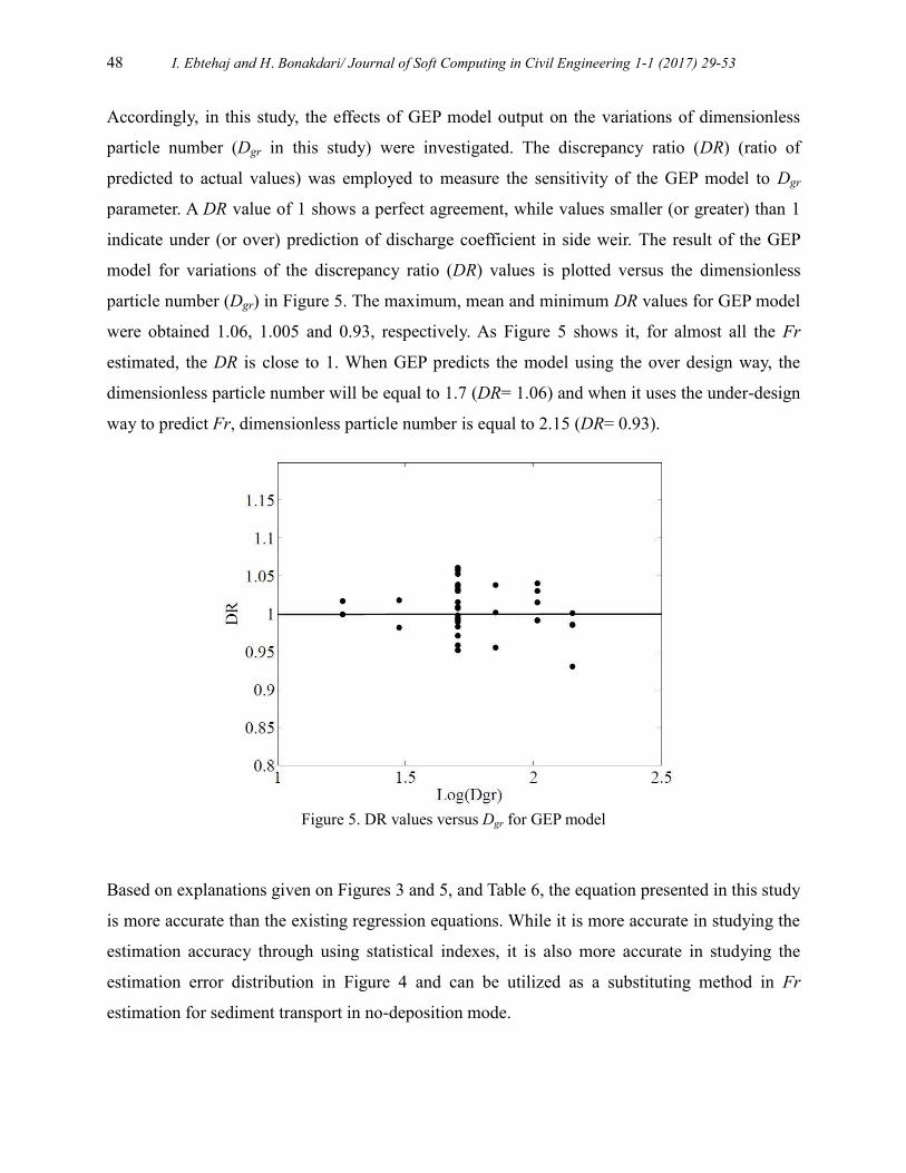
Accordingly, in this study, the effects of GEP model output on the variations of dimensionless

particle number (Dgr in this study) were investigated. The discrepancy ratio (DR) (ratio of

predicted to actual values) was employed to measure the sensitivity of the GEP model to Dgr

parameter. A DR value of 1 shows a perfect agreement, while values smaller (or greater) than 1

indicate under (or over) prediction of discharge coefficient in side weir. The result of the GEP

model for variations of the discrepancy ratio (DR) values is plotted versus the dimensionless

particle number (Dgr) in Figure 5. The maximum, mean and minimum DR values for GEP model

were obtained 1.06, 1.005 and 0.93, respectively. As Figure 5 shows it, for almost all the Fr

estimated, the DR is close to 1. When GEP predicts the model using the over design way, the

dimensionless particle number will be equal to 1.7 (DR= 1.06) and when it uses the under-design

way to predict Fr, dimensionless particle number is equal to 2.15 (DR= 0.93).

Figure 5. DR values versus Dgr for GEP model

Based on explanations given on Figures 3 and 5, and Table 6, the equation presented in this study

is more accurate than the existing regression equations. While it is more accurate in studying the

estimation accuracy through using statistical indexes, it is also more accurate in studying the

estimation error distribution in Figure 4 and can be utilized as a substituting method in Fr

estimation for sediment transport in no-deposition mode.


8. Conclusion

Transmitting flow from sewerage systems often contains suspended materials. Therefore, transporting suspended

materials and preventing their sedimentation are important matters in flow transport through sewerage networks.

Different methods have been presented for sediment transport in sewages, but due to the lack of recognition of

effective factors on sediment transport these methods show different results in different conditions. Hence, in recent

years, soft computations have been utilized in order to estimate densimetric Froude number (Fr) in these systems. In

this paper, with the use of presented model by Gene-expression programming (GEP), Fr has been estimated. In

order to present the effective factor on Fr estimation, six different models were presented. In these models, the effect

of movement, transport, sediment, transport mode and flow resistance parameters have been considered. After Fr

estimation, the precision of all sextet models has been studied. The results indicated that among the three parameters

provided by “Transport mode” group, the best and the worst accuracy were achieved by using d/R and D2/A

(respectively) as improper use of the parameters of this group, up to two-fold increase relative error. In addition to,

Also, with the constant parameters in the groups “transport”, “flow resistance” and “transport mode”, the parameter

d/D in all input combinations, leading to better results than when used Dgr as “sediment” parameter. Therefore, it

was revealed that the model which considers volumetric sediment concentration (CV), relative flow depth (d/R),

proportional average size of particles (d/D), overall friction factor (λs) for Fr estimation, shows the best results. The

presented model estimates Fr with an average error value about 2.82%. The comparison of existing methods

illustrated the high level of accuracy of Ebtehaj et al. (Eq. 3) method in comparison with others. It should not be

inappropriate use of GEP functions such as Eq. (4) results in weak performance of model. The presented model with

existing values was also studied and the results showed that in proportion with existing relations the model well

estimates the Fr. Incidentally making use of the proposed GEP-based technique in form of the most superlative

formulations has a dominant role to experience in the attaining astonishing and remarkable successes for real-world

application. Another plus aspect of this study is the use of extracted mathematical expressions as realistically

valuable technique for practical engineering as an alternative for existing methods.

Notation:

A Cross-sectional area of the flow

CV Volumetric sediment concentration


D Pipe diameter

d Median diameter of particle size

Dgr Dimensionless particle number

E(ij) Error of program i for fitness case j (Eq. 5)

Fr Densimetric Froude number

P Precision (Eq. 5)

P(ij) Value predicted by individual program i for fitness case j (Eq. 6)

R Hydraulic radius, Selection Range (Eq. 6)

s Specific gravity of sediment (=ρs/ρ)

V Velocity of flow

Vt Incipient flow velocity which follows from equation (2)

y Flow depth

λc Clear Water friction factor

λs Overall sediment friction factor

ψ Flow parameter

φ Transport parameter

References

Ab Ghani A (1993) Sediment transport in sewers. PhD Thesis, University of Newcastle Upon Tyne, UK

Ab Ghani A, Azamathulla HM (2011) Gene Experession Programming for Sediment Transport in Sewer

Pipe Systems. J Pipeline Syst Eng Pract 2(3):102-106

Ackers P (1991) Sediment aspects of drainage and outfall design. Proc Int Symp Environ Hydraul, Hong

Kong.

Ackers JC, Butler D, May RWP (1996) Design of sewers to control sediment problems. Report No.

CIRIA 141, Construction Industry Research and Information Association, London, UK

Ackers P, White WR (1973) Sediment transport; new approach and analysis. J Hydraul Div-ASCE.,

99(HY11):2041-2060

Ahmadianfar I, Adib A, Taghian M (2016) Optimization of multi-reservoir operation with a new hedging

rule: application of fuzzy set theory and NSGA-II. Appl Water Sci. doi:10.1007/s13201-016-0434-

z

Al-Abadi AM (2014) Modeling of stage–discharge relationship for Gharraf River, southern Iraq using

backpropagation artificial neural networks, M5 decision trees, and Takagi–Sugeno inference

system technique: a comparative study. Appl Water Sci. 1-14. doi:10.1007/s13201-014-0258-7

ASCE. (1970) Water pollution control federation: Design and construction of sanitary and storm sewers.

American Society of Civil Engineers Manuals and Reports on Engineering Practices, No. 37,

Reston, VA


Azamathulla HM, Ab Ghani A (2010) Genetic Programming to Predict River Pipeline Scour. J Pipeline

Syst Eng Pract 1(3):127-132

Azamathulla HM, Ab Ghani A, Fei SY (2012) ANFIS – based approach for predicting sediment transport

in clean sewer. J Appl soft Comput 12(3):1227-1230

Azamathulla HMd, Ahmad Z (2012) Gene-expression programming for transverse mixing coefficient. J

Hydrol 435(20):142-148

Azimi H, Bonakdari H, Ebtehaj I, Talesh SHA, Michelson D G, Jamali A (2017) Evolutionary Pareto

optimization of an ANFIS network for modeling scour at pile groups in clear water condition.

Fuzzy Set Syst 319:50-69.

Banasiak R (2008) Hydraulic performance of sewer pipes with deposited sediments. Water Sci Technol

57(11):1743-1748

Butler D, Clark RB (1995) Sediment management in urban drainage catchments. CIRIA Report No. 134,

Construction Industry Research and Information Association, London, UK.

Butler D, May R, Ackers J (2003) Self-cleansing sewer design based on sediment transport principles. J

Hydraul Eng 129(4):276-282.

BS8005-1. (1987) Sewerage Guide to New Sewerage Construction, British Standard Institution, London,

UK.

Chang CK, Azamathulla HM, Zakaria NA, Ab Ghani A (2012) Appraisal of soft computing techniques in

prediction of total bed material load in tropical rivers. J Earth Syst Sci 121(1):125-133

Ebtehaj I, Bonakdari H (2013) Evaluation of Sediment Transport in Sewer using Artificial Neural

Network. Eng Appl Comput Fluid Mech 7(3):382-392

Ebtehaj I, Bonakdari H (2014) Performance Evaluation of Adaptive Neural Fuzzy Inference System for

Sediment Transport in Sewers. Water Resour Manage 28(13):4765–4779

Ebtehaj I, Bonakdari H, Sharifi A (2014) Design criteria for sediment transport in sewers based on self-

cleansing concept. J Zhejiang Univ-Sci A 15(11):914-924

European Standard EN 752-4 (1997) Drain and sewer system outside building: Part 4. Hydraulic design

and environmental considerations, Brussels: CEN (European Committee for Standardization)

Gad MI, Khalaf S (2013) Application of sharing genetic algorithm for optimization of groundwater

management problems in Wadi El-Farigh, Egypt. Appl Water Sci 3(4):701-716

Gorai AK, Hasni SA, Iqbal J (2014) Prediction of ground water quality index to assess suitability for

drinking purposes using fuzzy rule-based approach. Appl Water Sci. doi:10.1007/s13201-014-

0241-3

Maghrebi MF, Givehchi M (2007) Using non-dimensional velocity curves for estimation of longitudinal

dispersion coefficient. Proceedings of the seventh international symposium river engineering, 16-

18 October, Ahwaz, Iran.

Ferreira C (2001) Gene Expression Programming: A New Adaptive Algorithm for Solving Problems.

Complex Syst 13(2):87–129

Ferreira C (2006) Gene Expression Programming: Mathematical Modeling by an Artificial Intelligence.

2nd

Edition, Springer-Verlag, Germany

Gan Z, Yang Z, Li G, Jiang M (2007) Automatic modeling of complex functions with clonal selection-

based gene expression programming. In Natural Computation, 2007. ICNC 2007. Third

International Conference on (Vol. 4, pp. 228-232). IEEE.

Graf WH, Acaroglu ER (1968) Sediment transport in conveyance systems. Bulletin IAHR, Part 1,

13(2):20-39.

Hsu K, Gupta VH, Sorroshian S (1995) Artificial neural network modeling of the rainfall-runoff process.

Water Resour Res 31(10):2517-2530

http://www.gene-expression-programming.com/webpapers/GEP.pdf

http://www.gene-expression-programming.com/books/index.asp


Isanta Navarro R (2013) Study of a neural network-based system for stability augmentation of an

airplane. Universitat Polite`cnica de Catalunya, Barcelona, pp. 77.

Jain A, Ormsbee LE (2002) Evaluation of short-term water demand forecast modeling techniques:

Conventional methods versus AI. J Am Water Works Ass 94(7):64-72

Jain A, Varshney AK, Joshi UC (2001) Short-term water demand forecast modeling at IIT Kanpur using

artificial neural networks. Water Resour Manage 15(5):299-321

Khan M., Azamathulla, HM, Tufail M, Ab Ghani A (2012) Bridge pier scour prediction by gene

expression programming. P ICE-Water Manage 165(9):481-493

Khoshbin F, Bonakdari H, Ashraf Talesh SH, Ebtehaj I, Zaji AH, Azimi H (2016) Adaptive neuro-fuzzy

inference system multi-objective optimization using the genetic algorithm/singular value

decomposition method for modelling the discharge coefficient in rectangular sharp-crested side

weirs. Eng Optimiz 48(6):933-948.

Koza JR (1992) Genetic programming: On the programming of computers by means of natural selection,

MIT Press, Cambridge, MA, USA

Legates DR, McCabe JR (1999) Evaluating the use of goodness-of-fit measures in hydrologic and

hydroclimatic model validation. Water Resour Res 35(1):233-241

Lysne DK (1969) Hydraulic design of self-cleaning sewage tunnels. J Sanitary Eng Div-ASCE

95(SA1):17-36

Macke E (1982) About sediment at low concentrations in partly filled pipes. Mitteilungen, Leichtweiss

institut fur Wasserbau der technischen Universitat Braunschweig, Heft 71:1-151 (In Germany)

May RWP (1982) Sediment transport in sewers. Hydraulic Research Station, Wallingford, England,

Report IT 222

May RWP, Ackers JC, Butler D, John S (1996) Development of design methodology for self-cleansing

sewers. Water Sci Technol 33(9):195-205

May RWP, Brown PM, Hare GR, Jones KD (1989) Self-cleansing condition for sewers carrying

sediment. Hydraulic Research Ltd (Wallingford), Report SR 221

Mayerle R (1988) Sediment transport in rigid boundary channels. PhD Thesis, University of Newcastle

Upon Tyne, UK

Mayerle R, Nalluri C, Novak P (1991) Sediment transport in rigid bed conveyance. J Hydraul Res

29(4):475-495

Mondal SK, Jana S, Majumder M, Roy D (2012) A comparative study for prediction of direct runoff for a

river basin using geomorphological approach and artificial neural networks. Appl Water Sci 2(1):1-

13

Nalluri C (1985) Sediment transport in rigid boundary channels. Proceeding Euromech 192: Transport of

Suspended Solids in Open channels, Neubiberg, Germany

Nalluri C, Ab Ghani A (1993) Bed load transport without deposition in channel of circular section.

Proceeding of the sixth international conference on Urban Storm Drainage, Niagara Falls, Canada

Nalluri C, Ab Ghani A (1996) Design option for self-cleansing storm sewers. Water Sci Technol

33(9):215-220

Nalluri C, Ab Ghani A, El-Zaemey AK (1994) Sediment transport over deposited beds in sewers. Water

Sci Technol 29(1-2):125-133

Novak P, Nalluri C, (1975) Sediment transport in smooth fixed bed channels. J Hydraul Div-ASCE

101(9):1139-1154

Ota JJ, Nalluri C (1999) Graded sediment transport at limit deposition in clean pipe channel. 28th Int

Assoc Hydro-Environ Eng Res, Graz, Austria

Ota JJ, Perrusquía GS (2013).Particle velocity and sediment transport at the limit of deposition in sewers.

Water Sci. Technol 67(5):959-967.


Pedroli R (1963) Bed load transportation in channels with fixed and smooth inverts. PhD Thesis, Scuola

Politecnica Federale, Zurigo, Switzerland

Rajurkar MP, Kothyari UC, Chaube UC (2004) Modeling of the daily rainfall-runoff relationship with

artificial neural network. J Hydrol 285(1):96-113.

Rezaei H, Rahmati M, Modarress H (2017) Application of ANFIS and MLR models for prediction of

methane adsorption on X and Y faujasite zeolites: effect of cations substitution. Neural Comput

Appl 28(2):301-312.

Safari MJS, Aksoy H, Unal NE, Mohammadi M (2017) Non-deposition self-cleansing design criteria for

drainage systems. J Hydro-environ Rese 14:76-84.

Singh R, Vishal V, Singh T (2012) Soft computing method for assessment of compressional wave

velocity. Sci Iran 19:1018–1024

Singh R, Vishal V, Singh T, Ranjith P (2013) A comparative study of generalized regression neural

network approach and adaptive neuro-fuzzy inference systems for prediction of unconfined

compressive strength of rocks. Neural Comput Appl 23:499–506

Vongvisessomjai N, Tingsanchali T, Babel MS (2010) Non-deposition design criteria for sewers with

part-full flow. Urban Water J 7(1):61-77

Documents

No deposition Sediment Transport in Sewers Using Gene ...jsoftcivil.com/article_46845_939933649999c0af310c3f047268182b.pdf · No-deposition Sediment Transport in Sewers Using Gene