Embed Size (px)
Citation preview

Louisiana State UniversityLSU Digital Commons
LSU Historical Dissertations and Theses Graduate School
1986
Mud Deposition at the Shoreface: Wave andSediment Dynamics on the Chenier Plain ofLouisiana.George Paul KempLouisiana State University and Agricultural & Mechanical College
Follow this and additional works at: https://digitalcommons.lsu.edu/gradschool_disstheses
This Dissertation is brought to you for free and open access by the Graduate School at LSU Digital Commons. It has been accepted for inclusion inLSU Historical Dissertations and Theses by an authorized administrator of LSU Digital Commons. For more information, please [email protected].
Recommended CitationKemp, George Paul, "Mud Deposition at the Shoreface: Wave and Sediment Dynamics on the Chenier Plain of Louisiana." (1986).LSU Historical Dissertations and Theses. 4305.https://digitalcommons.lsu.edu/gradschool_disstheses/4305

INFORMATION TO USERS
While the most advanced technology has been used to photograph and reproduce this manuscript, the quality of the reproduction is heavily dependent upon the quality of the material submitted. For example:
• Manuscript pages may have indistinct print. In such cases, the best available copy has been filmed.
• Manuscripts may not always be complete. In such cases, a note will indicate that it is not possible to obtain missing pages.
• Copyrighted material may have been removed from the manuscript. In such cases, a note will indicate the deletion.
Oversize materials (e.g., maps, drawings, and charts) are photographed by sectioning the original, beginning at the upper left-hand comer and continuing from left to right in equal sections with small overlaps. Each oversize page is also film ed as one exposure and is available, for an additional charge, as a standard 35mm slide or as a 17”x 23” black and white photographic print.
Most photographs reproduce acceptably on positive microfilm or microfiche but lack the clarity on xerographic copies made from the microfilm. For an additional charge, 35mm slides of 6”x 9” black and white photographic prints are available for any photographs or illustrations that cannot be reproduced satisfactorily by xerography.
Reproduced with permission of the copyright owner. Further reproduction prohibited without permission.

Reproduced with permission of the copyright owner. Further reproduction prohibited without permission.

8710568
K em p, G eorge Paul
MUD DEPOSITION AT THE SHOREFACE: WAVE AND SEDIMENT DYNAMICS ON THE CHENIER PLAIN OF LOUISIANA
The Louisiana State University and A gricu ltura l and M echanical Col. Ph.D.
UniversityMicrofilms
International 300 N. Zeeb Road, Ann Arbor, Ml 48106
Copyright 1987
by
Kemp, George Paul
All Rights Reserved
1986
Reproduced with permission of the copyright owner. Further reproduction prohibited without permission.

Reproduced with permission of the copyright owner. Further reproduction prohibited without permission.

PLEASE NOTE:
In all c a ses this material has been filmed in the best possible way from the available copy. Problems encountered with this docum ent have been identified here with a ch eck mark V .
1. Glossy photographs or p a g e s .
2. Colored illustrations, paper or print_______
3. Photographs with dark background i / ^
4. Illustrations are poor co p y _______
5. Pages with black marks, not original co p y _______
6. Print show s through as there is text on both sides of p a g e ________
7. Indistinct, broken or small print on several pages
8. Print exceeds margin requirem ents_______
9. Tightly bound cop y with print lost in sp in e________
10. Computer printout pages with indistinct print_______
11. P age(s)_____________ lacking when material received, and not available from school orauthor.
12. P age(s)_____________ seem to b e missing in numbering only as text follows.
13. Two pages num bered . Text follows.
14. Curling and wrinkled p a g e s_______
15. Dissertation contains pages with print at a slant, filmed a s received t /
16. Other_______________________________________________________________________________
UniversityMicrofilms
International
Reproduced with permission of the copyright owner. Further reproduction prohibited without permission.

Reproduced with permission of the copyright owner. Further reproduction prohibited without permission.

MUD D E PO SIT IO N AT T H E SH O R E FA C E : W AVE AND SED IM EN T D Y N A M ICS
ONT H E C H E N IE R PLA IN O F L O U ISIA N A
A Dissertation
Submitted to the Graduate Faculty of the Louisiana State University and
Agricultural and Mechanical College in partial fulfillment of the
requirements for the degree of Doctor of Philosophy
in
The Department of Marine Sciences
byG. Paul Kemp
B.S., Cornell University, 1975 M.S., Louisiana State University, 1978
December 1986
Reproduced with permission of the copyright owner. Further reproduction prohibited without permission.

©1987
GEORGE PAUL KEMP
All Rights Reserved
Reproduced with permission of the copyright owner. Further reproduction prohibited without permission.

A C K N O W L E D G E M E N T S
Support for this project was provided by the Louisiana Sea Grant
University Program, a part of the National Sea Grant University Program
maintained by the National Oceanic and Atmospheric Administration of the
U.S. Department o f Commerce. Additional field support was generously
furnished by the Louisiana Universities Marine Consortium (LUMCON),
and the U.S. Army Corps of Engineers staff at Freshwater Bayou Canal
Lock. .
John Wells introduced me to the mudflat problem and supervised this
research. Dag Nummedal participated actively in the field program, and was
unfailing in his encouragement. William Wiseman, Jr., patiently schook i
me in the art of time-series analysis. Charles Adams, Jr., gave invaluable
assistance with boundary layer theory. James Coleman and James Gosselink
contributed sound advice throughout an unorthodox student career. W.
David Constant assisted ably as a member of the examining committee.
Floyd Demers, Annie McK. Prior, and Gerald McHugh at the Coastal
Studies Institute, and Mike DeTraz of LUMCON, were instrumental in
bringing this project to a successful completion. Celia Harrod and Kerry
Lyle provided much needed assistance with the graphics. Scott Dinnel, Ivor
LI. van Heerden, Lauro Calliari, and Allison Drew deserve recognition
among the many students who contributed.
A special thanks is extended to my understanding colleagues at
Groundwater Technology, Inc., to the Joseph Lipsey, Sr., Scholarship award
committee, and to Geraldine Newman at the Department of Marine Sciences.
The greatest measures of appreciation go to my parents, and to Linda
Fowler, my partner in all endeavors.
ii
Reproduced with permission of the copyright owner. Further reproduction prohibited without permission.
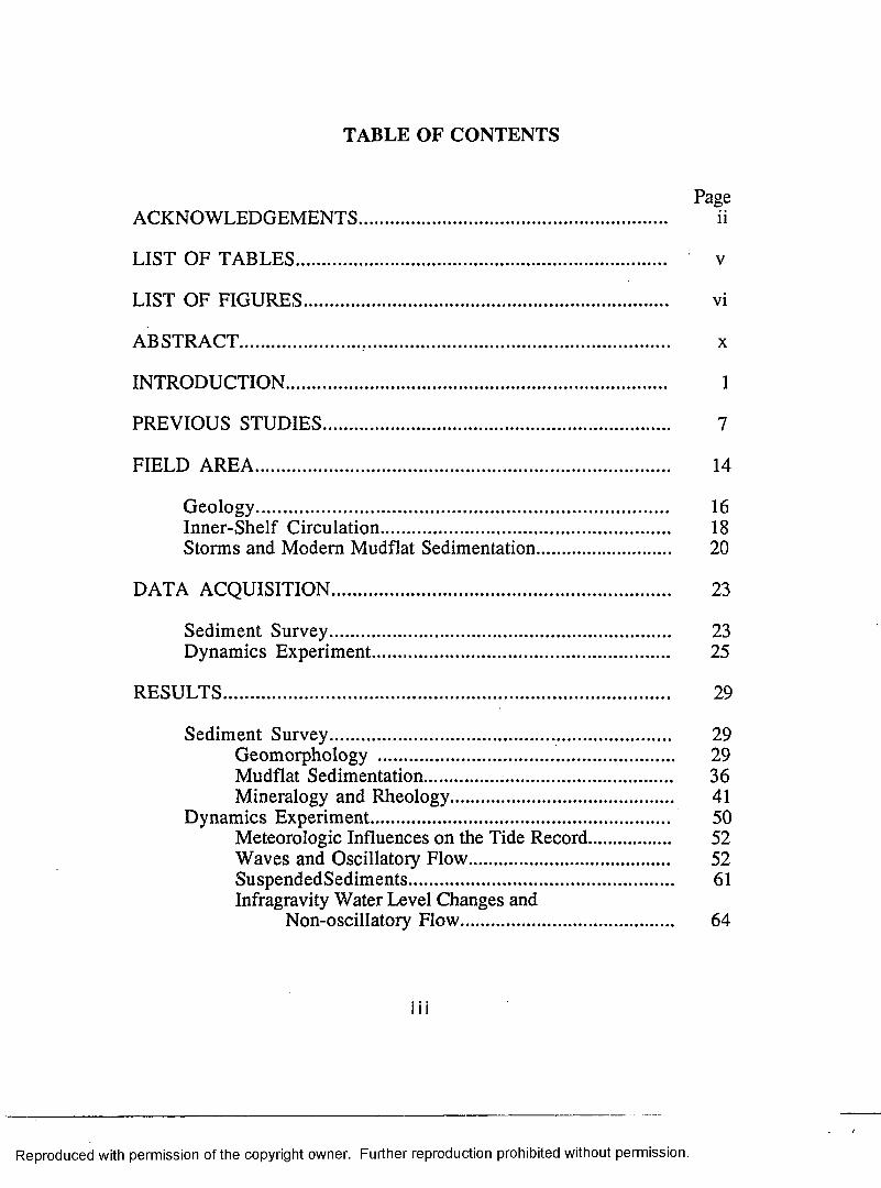
TABLE OF CONTENTS
PageACKNOW LEDGEM ENTS...................................................................... ii
LIST OF TABLES.................................................................................... v
LIST OF FIGURES................................................................................... vi
A BSTRACT........................... x
INTRODUCTION...................................................................................... 1
PREVIOUS STUDIES............................................................................... 7
FIELD A REA .............................................................................................. 14
G eology.............................................................................................. 16Inner-Shelf C irculation.................................................................. 18Storms and M odem Mudflat Sedimentation.............................. 20
DATA ACQUISITION............................................................................. 23
Sediment Survey............................................................................. 23Dynam ics Experim ent ........................................................... 25
RESU LTS..................................................................................................... 29
Sediment Survey............................................................................. 29Geomorphology ................................................................... 29M udflat Sedimentation........................................................ 36Mineralogy and Rheology.................................................. 41
Dynamics Experim ent.................................................................... 50Meteorologic Influences on the Tide Record.................. 52Waves and Oscillatory Flow............................................. 52SuspendedSediments............................................................ 61Infragravity W ater Level Changes and
Non-oscillatory Flow................................................ 64
Reproduced with permission of the copyright owner. Further reproduction prohibited without permission.

DISCUSSION 80
Formation and Transport of Fluid M ud...................................... 85Kinematics of Fluid Mud Deposition at the Shoreface............... 91Shelf Sediment Dispersal................................................................ 100Future Chenier Plain Progradation............................................... 102Implications for Other Coasts and the Geologic Record 103
CONCLUSIONS.......................................................................................... 106
BIBLIOGRAPHY......................................................................................... I l l
APPEND ICES.............................................................................................. 133
A. Beach Profiles.......................................................................... 133B. Program for Grant-Madsen Boundary Layer Closure 142
V ITA .................................................................................................................. 148
APPROVAL SHEETS............................................................................... 149
iv
Reproduced with permission of the copyright owner. Further reproduction prohibited without permission.

LIST OF TABLES
Table . Page
1. Chenier Plain Shoreline Characteristics...................................... 31
2. Clay Mineral Abundances.............................................................. 46
3. Sea and Swell Wave Statistics....................................................... 53
4. Total Suspended Sediment............................................................. 62
5. W ater Level Variance Below 0.005 cps....................................... 67
6. Non-Oscillatory Onshore-Offshore Flow.................................... 70
7. Steady Alongshore Flow............................................................... 73
8. Characteristic Alongshore Velocity Profile Parameters 78
9. Grant-Madsen Boundary Layer Model Results........................... 88
v
Reproduced with permission of the copyright owner. Further reproduction prohibited without permission.

LIST OF FIGURES
Figure Page
1. Location of chenier plain study area............................................ 6
2. Map of study area, showing major shoreline featuresand beach survey stations.................................................. 15
3. Cross-section of shoreface at station 6, showingdeployment of sensors during cold frontexperim ent............................................................................ 26
4. Nearshore surficial sediments and bathymetry in thestudy area.............................................................................. 30
5a-b. Muddy shoreface at station 7 (5a); reactivatedchenier beach (station 2) at Cheniere au Tigre (5b)........ 32
6a-b. Time-lapse views of the vegetated mudflat mapped by Morgan et al. (1953) at station 3; eroding marsh scarp, May, 1982 (6a), replaced by clastic washover beach, May, 1985 (6b)......................... 34
7. Bar migration at Tigre Point (station 4)..................................... 35
8. Oblique aerial view of western limb of large mud barformed in Spring, 1982, between stations 7 and 8.......... 37
9. Profile time-series of mudflat accretion and erosionat station 8, February - July, 1981................................... 37
lOa-b. Shoreface mud at station 7; Freshly-deposited fluidmud, Spring 1982 (10a); eroding surface showingdevelopment o f shore-normal flutes 5 monthslater (10b).............................................................................. 38
11. Log of vibracore from marsh now covering mudflatdescribed by Morgan et al. (1953) west of Cheniere au Tigre at station 3............................................ 40
vi
Reproduced with permission of the copyright owner. Further reproduction prohibited without permission.

12a-c. Bedding structure in radiograph positives of mudflatsequences............................................................................... 42
13. Texture and bulk density changes with depth in uppermeter of newly deposited m udflat.................................... 43
14. X-ray diffractograms of smears from the <1 jx fractionof mudflat sediments treated as indicated........................ 45
15. Shear stress-strain rate plot from capillaryviscometer measurements on mudflat sediment 48
16. Fluid mud yield strength plotted as a function ofsediment concentration (from McCave 1984)................. 49
17. Winds and tides during cold front experiment,1 0 - 1 3 December, 1982..................................................... 51
18. Representative energy density spectra from 20 minutepressure and flowmeter time-series for pre-frontal, frontal, and post-frontal runs............................................ 55
19a-b. Concurrent spectra, and cross-spectral estimates of coherence and phase for records from run 3; between seaward and landward sensors located 10 m apart (19a), and between near-surface and near-bottom flowmeters (19b)............................. 57
20. The areas of application of the several wave theoriesas a function of H/d and d/L (from Komar 1976)........... 59
21a-c. Relationships between wave parameters determined from the spectra and cross-spectra, and those predicted by shallow water LWT; wavelength (21a), and orbital velocity (21b)................................................... 60
22. Mean suspended sediment concentrations fromrepresentative pre-frontal, frontal, and post-frontal runs............................................................................. 63
vii
Reproduced with permission of the copyright owner. Further reproduction prohibited without permission.

23. Relationship between vertical sediment concentrationgradient and the relative heights of sea andsw ell........................................................................................ 65
24. Low frequency water level and onshore-offshoreflowmeter data from frontal run 3.................................... 68
25. Sequence of vertical velocity profiles during onshore-offshore flow event in run 3.............................................. 71
26. Low frequency water level and alongshore flowmeterdata from frontal run 5 ....................................................... 74
27. Characteristic logarithmic alongshore velocityprofiles for frontal runs 4 and 5, and post-frontalrun 8........................................................................................ 79
28. B-L-S model for sorting of cohesive and non-cohesivesediments in the boundary layer of a turbidity current
(from Stow and Bowen 1980)............................................ 82
29. Generalized shoreface geometry, showing slopes usedin determining standing wave node position, and changes in the cross-section affecting crossshore velocities...................................................................... 94
30a-b. Cross-shore trends in low-frequency flow understanding waves (30a), and bed shear stress dueto waves attenuated at a constant H/d ratio of0.2 (30b).................................................................................. 95
A -l. Station 1 profile sequence................................................................ 134
A-2. Station 2 profile.sequence.......................... 135
A-3. Station 3 profile.sequence................................................................ 136
A-4. Station 4 profile sequence................................................................ 137
A-5. Station 5 profile.sequence............................................................... 138
A-6. Station 6 profile sequence................................................................ 139viii
Reproduced with permission of the copyright owner. Further reproduction prohibited without permission.

A-7. Station 7 profile sequence................................................................. 140
A-8. Station 8 profile sequence................................................................. 141
ix
Reproduced with permission of the copyright owner. Further reproduction prohibited without permission.

A B STR A C T
Sedimentological data, and high-resolution current velocity time-
series were acquired nearshore along the muddy coast of Louisiana's chenier
plain. Results suggest that the 2 to 10 cm thick, laminated and graded
silt/shell + mud beds which characterize shoreface mudflat sedimentation
form through intermittent dumping of fluid mud suspensions. Cohesive and
non-cohesive sediments are first separated and concentrated by shear within a
wave boundary layer (WBL). Rapid sedimentation, or "freezing", of the
mud fraction occurs when the yield strength of the fluid mud suspension
equals that of the WBL shear stress.
Incident waves were well described by shallow water linear wave
theory, but exhibited the progressive nearshore attenuation and absence of
breaking characteristic of muddy shorelines. An onshore decrease in wave
shear stress results, which is the reverse of that on surf-dominated coasts.
Fluid mud layers, characterized by significant yield strength, are proposed to
form when high concentrations of suspended sediments are introduced
nearshore, but are prevented from depositing by WBL shear stresses close to
the bed. In cross-section, WBL sorting causes a near-bottom discontinuity in
sediment concentration, and the associated vertical yield strength gradient.
Expanded spatially, this point of weakness forms a plane along which the
fluid mud layer can move in response to shear exerted at its upper margin by
an accelerating flow.
Adjustment of the steady alongshore current velocity profile to the
fluid mud layer restricts coastwise sediment transport. Significant cross
shore transport of fluid mud may occur, however, under the influence of
unsteady flows. Such low-frequency flows were found to be associated with
x
Reproduced with permission of the copyright owner. Further reproduction prohibited without permission.

shore-amplified water level oscillations which have characteristics of a
standing wave with an antinode at the shoreline. The onshore decreasing
wave shear stress gradient leads to preferential deposition at the shoreface.
Widespread renewal of chenier plain shoreline advance through
mudflat accretion is predicted when the Atchafalaya delta, now forming 100
km to the east in Atchafalaya Bay, emerges on the inner shelf, and the
nearshore supply of fine-grained sediment is dramatically increased.
Reproduced with permission of the copyright owner. Further reproduction prohibited without permission.

IN T R O D U C T IO N
The past 15 years have witnessed a growth in knowledge about silt and
clay sedimentation which was recently likened to an "information explosion"
(Stow and Piper 1984). An early casualty of this "explosion" was the belief
that marine muds accumulate only in quiescent environments, isolated from
currents exceeding a few cm-s_l . Nowhere does the "quiescent
environment" paradigm contrast more with what is observed than on a
significant fraction of the world's coastlines where fine-grained sediment is
deposited at the beach face itself. There, mud sedimentation occurs in non-
estuarine settings exposed to high-velocity wave-generated flows, in addition
to significant steady currents (Dolan et al. 1972, Rine and Ginsburg 1985).
In most locations it alternates spatially and temporally with the more familiar
coarse-grained clastic deposition (Delaney 1963, Wells and Coleman 1981a,
b). Elsewhere, it appears to occur only during the high energy conditions
accompanying storms (Morgan et al. 1958, Nair 1976, Martins et al. 1979).
Modem mud coasts can provide guidance in the interpretation of
ancient sequences in which marine shales are observed to merge laterally or
vertically into non-marine deposits without the transitional beach and tidal
facies normally considered indicative of shoreline processes (Rine and
Ginsburg 1985, Walker and Harms 1971,1976; Keulegan and Krumbein
1949, Moore 1929). An understanding of the hydrodynamic and
oceanographic factors which give rise to any muddy shoreface would greatly
improve the utility of a facies model of widespread applicability. Unlike the
dynamics of littoral onshore-offshore clastic sediment transport, which have
been studied for nearly a century (Cornish 1898), those pertaining to
1
Reproduced with permission of the copyright owner. Further reproduction prohibited without permission.
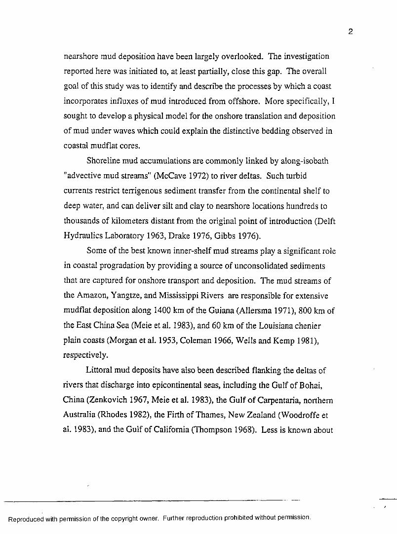
2
nearshore mud deposition have been largely overlooked. The investigation
reported here was initiated to, at least partially, close this gap. The overall
goal of this study was to identify and describe the processes by which a coast
incorporates influxes of mud introduced from offshore. More specifically, I
sought to develop a physical model for the onshore translation and deposition
of mud under waves which could explain the distinctive bedding observed in
coastal mudflat cores.
Shoreline mud accumulations are commonly linked by along-isobath
"advective mud streams" (McCave 1972) to river deltas. Such turbid
currents restrict terrigenous sediment transfer from the continental shelf to
deep water, and can deliver silt and clay to nearshore locations hundreds to
thousands of kilometers distant from the original point of introduction (Delft
Hydraulics Laboratory 1963, Drake 1976, Gibbs 1976).
Some of the best known inner-shelf mud streams play a significant role
in coastal progradation by providing a source of unconsolidated sediments
that are captured for onshore transport and deposition. The mud streams of
the Amazon, Yangtze, and Mississippi Rivers are responsible for extensive
mudflat deposition along 1400 km of the Guiana (Allersma 1971), 800 km of
the East China Sea (Meie et al. 1983), and 60 km of the Louisiana chenier
plain coasts (Morgan et al. 1953, Coleman 1966, Wells and Kemp 1981),
respectively.
Littoral mud deposits have also been described flanking the deltas of
rivers that discharge into epicontinental seas, including the Gulf of Bohai,
China (Zenkovich 1967, Meie et al. 1983), the Gulf of Carpentaria, northern
Australia (Rhodes 1982), the Firth of Thames, New Zealand (Woodroffe et
al. 1983), and the Gulf of California (Thompson 1968). Less is known about
Reproduced with permission of the copyright owner. Further reproduction prohibited without permission.

3
apparently non-deltaic coastal mudflat deposition reported adjacent to lagoon
systems on the south-west coast of India (Nair 1976) and on the Rio Grande
do Sul coast of southern Brazil (Delaney 1963, Martins et al. 1979).
These sources document littoral mud deposition in all tide ranges and
wave energy regimes. The coastal features formed exhibit a spectrum of
morphologies. Ephemeral mud "arcs", spits and bars with a few square
kilometers of subaerial expression have been described from Louisiana
(Morgan et al. 1958, Wells and Kemp 1981). In contrast, migratory "mud
banks" a hundred times larger have been tracked for decades off the coast of
Surinam and the Guianas (NEDECO 1968, Rine and Ginsburg 1985).
Elsewhere, coastal mud deposits have been designated only with the generic
terms "flat" or "tidal flat", suggesting that features with discrete alongshore
boundaries are not observed.
While our knowledge of the processes important to fine-grained
sedimentation under waves is growing rapidly, lessons learned in the
laboratory about the complexity of this subject have led some to believe that
little might be gained from field research. The singular investigation by
Wells and Coleman (1981a, b) of the relationship between shallow-water
waves and mud suspension on the coast of Surinam suggests, however, that
such work can provide insights which might not be recognized at laboratory
scales.
The eastern margin of Louisiana's chenier plain coast today offers an
ideal location for study of the dynamics of fine-grained sediment deposition
and erosion in a wave-dominated environment (Fig. 1). This area is
presently receiving an influx of mud from the Atchafalaya River, a
Mississippi distributary now building a delta lobe in a bay 100 km to the east
Reproduced with permission of the copyright owner. Further reproduction prohibited without permission.
/

4
(van Heerden et al. 1981). In some locations, fine-grained sediments
accumulate near shore under conditions similar to those described by Wells
and Coleman (1981a) in a process which appears to involve deposition from
highly concentrated mud-water suspensions or fluid mud. Nearby, however,
muddy shorelines exposed to the same wind and wave conditions are
erosional, while on others, normal surf zone processes and sandy beach
sedimentation prevail (Wells and Kemp 1981, Kaczorowski and Gemant
1980).
A two-staged approach was adopted to meet the objectives. First, a
survey of offshore bathymetry and sediment composition was combined with
a 2.5 year beach profiling program to supply regional coverage of the
temporal and spatial patterns of sand and mud deposition along the 30 km of
coast indicated in Figure 1. Cores from marsh, mudflat, and nearshore
environments were analyzed to provide information on depositional
processes, as well as the mineralogy and rheology of the mud itself.
Second, a dynamics experiment was conducted during the passage of a
winter cold front, when a range of energy conditions, typical to this coast,
could be examined and compared over a short time interval. Rapid-response
flowmeters, pressure sensors, and a multi-level suspended sediment sampler
were deployed in the shallow nearshore zone where mud deposition occurs.
This equipment was used to record wave characteristics, and to monitor
suspended sediment concentrations and flow velocities at various elevations
above the bed.
Evidence of major depositional events was acquired during the long
term monitoring program. Although significant mud sedimentation did not
take place during the four day period of the dynamics experiment, analysis of
Reproduced with permission of the copyright owner. Further reproduction prohibited without permission.
/

the time-series records yielded new insight into the nature of nearshore fine
grained sediment transport under waves.
Reproduced with permission of the copyright owner. Further reproduction prohibited without permission.

6
9.
I
c m eo
ooeCM0)
CO0CO> .
•O13w
oeo "co0CM CL
0) k -0
‘c0
-CO*♦—ocoCOoo
• —Ioo ,e T~COCD 0
k _3o>
'l l
Reproduced with permission of the copyright owner. Further reproduction prohibited without permission.

PR E V IO U S STU D IES
Even a brief survey of the literature reveals that the mechanics which
govern deposition of fine-grained sediments close to shore in the presence of
waves are largely unknown (Wells and Kemp 1985). The mere presence of
mud at the shoreface is troubling, as it appears to violate the consensus of
nearly a century of work establishing the preferential onshore transport of
the coarsest sediment fraction in clastic settings (Cornish 1898). The current
lack of understanding stems, first, from the absence of a general theory
relating mud deposition to fluid and sediment parameters, and, second, from
a paucity of field data. I. N. McCave (1984) addressed both of these factors
when he stated in a recent review that:
"there are no good ways of predicting the state of aggregation of polydisperse, multimineralic suspensions . . . , thus in natural situations empiricism reigns, but based on very few measurements".
Muddy coasts pose unique difficulties for researchers not only in the
theoretical sense, but also from the standpoint of logistics and
instrumentation. The development of new sensors, continued progress in the
laboratory, and an increased awareness of the disparity between what is
known about littoral sand and mud transport, have provided new impetus for
field efforts.
Gibbs (1970,1976) inferred from work in the vicinity of the Amazon
River mouth that a nearshore concentration of fine-grained sediments
occurred down coast through an Ekman-type coastal upwelling process.
Suspended sediments introduced from the Amazon are initially carried
7
Reproduced with permission of the copyright owner. Further reproduction prohibited without permission.

8
offshore and the sand fraction is deposited relatively close to the river mouth.
The great majority of the suspended load is, however, deflected to the west
by the Guiana Current. There, it becomes concentrated in bottom waters
with a significant shoreward velocity component which returns only the clay
fraction to the coast.
Van Straaten and Kuenen (1958) and Postma (1961) provided the first
physical model to account for the selective nearshore deposition of fine
grained sediments in a coastal marine setting, albeit one dominated by tidal
rather than wave generated flows. On the North Sea tidal flats studied,
deposits of mud were restricted to the higher elevation surfaces which
experienced only the final stages of the flood tidal current. These workers
developed the well known "scour-lag" hypothesis to explain this size
segregation. In it, they proposed that fine-grained sediments which settled
from the waning flood current and during slack tide formed deposits
sufficiently competent to resist removal by the subsequent ebb tidal scour.
These models provide an indication of the span of spatial and temporal scales
at which processes important to nearshore mud deposition can be expected to
operate, but do not specifically address the basic dynamics problem at the
shoreface, that is, how mud is deposited under waves.
The limited data available suggests that the presence of gel-like fluid
mud is characteristic of most open littoral settings where significant
shoreface deposition occurs (Morgan et al. 1953, Delft Hydraulics
Laboratory 1962, NEDECO 1965,1968; Zenkovitch 1967, Nair 1976,
Martins et al. 1979, Wells and Kemp 1985). This term has been loosely
applied to unconsolidated clay and silt suspensions with sediment
concentrations ranging from 10 to 300 g-1"1 (Einstein and Krone 1962).
Reproduced with permission of the copyright owner. Further reproduction prohibited without permission.
/

9
Chronic channel siltation associated with the occurrence of fluid mud
in San Francisco Bay led Einstein and Krone (1962) to conduct a classic
series of laboratory experiments on the modes of cohesive sediment transport
in salt water. Suspensions with salinities of l ° / o o and greater were found to
be of sufficient ionic strength to ensure that collisions between clay particles
would result in aggregates with lasting bonds. They proposed that fluid mud
forms from coagulation of dispersed fine-grained sediments in a flocculation
process involving collisions caused by both Brownian motion and fluid shear.
In the dispersed suspension, away from the bed, collisions between
particles take place primarily as a consequence of Brownian motion. Closer
to the bed, however, where both the particle population and the range of
particle sizes are greater, Einstein and Krone (1962) showed that local shear
could cause collisions at a rate far greater than Brownian motion alone.
Under these conditions large floes have a high probability of collision with
small ones and thereby continue to grow in size as they fall toward the bed.
The maximum size attainable by cohesive particles in the suspension is
thought to be determined by a complex and largely unknown interplay
between settling velocity, shear at the bed, and the strength of aggregate
bonds (McCave 1984). Einstein and Krone (1962) proposed that destruction
of floes by shear stress near the bed might return disaggregated particles to
the suspension and thereby restrict clay sedimentation.
Stow and Bowen (1980) suggest from their examination of silt
laminated turbidite muds that shear within the bottom boundary layer may
indeed act to sort silts and clays by concentrating clays in suspension while
allowing silts to deposit. In order to explain the graded and laminated silt-
mud couplets they observed, they proposed that at some critical
Reproduced with permission of the copyright owner. Further reproduction prohibited without permission.

10
concentration, shear is "overcome" and clays deposit rapidly as a blanket
over the silt laminae. Rine and Ginsburg (1985) found silt and clay couplets
in radiographs of Surinam mudflat deposits and have proposed that a similar
sorting process may operate in this coastal setting. No mechanism was
identified in either study to explain the required rapid clay deposition. More
than 40 years ago, however, Einstein (1941) explained sudden deposition, or
"freezing", of mud-charged subaqueous underflows as a consequence of the
tendency for such suspensions to acquire internal, or yield, strength in excess
of the shear stress applied.
It has long been known from viscometer measurements, that clay
suspensions in the fluid mud range behave as plastic solids rather than true
fluids (Bingham 1922, p. 215). As such, they are characterized by a capacity
to resist deformation up to some critical level of imposed shear stess
(Einstein 1941, Einstein and Krone 1962). The magnitude of the applied
stress required to initiate flow, or conversely, the level below which flow
ceases, defines the yield strength of the suspension. Krone (1962) found that
the yield strength of fluid mud from San Francisco Bay increased in
proportion to the sediment concentration raised to the power of 2.5. The
results of subsequent work on harbor muds from other locations suggest that
this empirical relationship may have broad applicability (Owen 1975,
Hydraulic Research Station 1979).
Because of the cohesive nature of the clay particles, deposits formed
from fluid mud suspensions produce beds which also exhibit non-Newtonian
rheological characteristics (Faas 1981). Maa and Mehta (in press) have
recently prepared a useful review of the extensive engineering literature on
this topic, which is briefly summarized here.. Beds of cohesive sediments
Reproduced with permission of the copyright owner. Further reproduction prohibited without permission.

11
respond to wave-induced shear in a complex manner which ranges from
elastic deformation to mass erosion (Alishahi and Krone 1964, Migniot
1968). Orbital motion and pressure oscillations associated with surface
waves have been observed to cause horizontal and vertical displacements at
and below the mudline both in the laboratory (Lhermitte 1960, Migniot
1968, Doyle 1973), and in the field (Tubman 1977). Furthermore, response
to one set of wave conditions may change with time. Mud beds "soften"
under cyclic loading (Thiers and Seed 1968, Schuckman and Yamamoto
1982) or suddenly liquify when pore pressures build beyond some critical
point (Turcotte et al. 1984).
The work performed by waves at and below the mudline effectively
dissipates wave energy, thereby attenuating wave heights at a far greater rate
than does normal friction over a consolidated sand bed. To explain wave
damping observed over the "mud hole", a region of fluid mud located
offshore of the central Louisiana coast, Gade (1958) provided an analytical
solution for the dissipation of wave energy by a deformable mud bed. In this
case, the bed was considered a viscous fluid. Since then, other analyses have
assumed bed response to be elastic (Gade 1959, Mallard and Dalrymple 1977,
Dawson 1980) or viscoelastic (Tubman 1977, Macpherson 1980, Hsiao and
Shemdin 1980, Maa 1986).
The study of Wells and Coleman (1981a) was the first to address the
effect of shoaling waves on mud suspension and transport nearshore.
Working along the coast of Surinam, they observed not only attenuation as
waves propagated over a gently sloping (0.0005) bottom blanketed with fluid
mud, but also a deformation of the characteristic wave profile from
sinusoidal in deep water to the steep, symmetrically crested, flat-troughed
Reproduced with permission of the copyright owner. Further reproduction prohibited without permission.
/

12
shape best described by solitary wave theory. Plunging breakers were
observed at mud-free interbank locations, but at stations fronted by fluid
mud, the long-crested solitary-like waves disappeared completely before
reaching the shoreline. Wave height decreased with water depth at a constant
ratio (H/d) of 0.23, far below 0.78, the critical value at which breaking can
theoretically occur (McGowan 1894). By monitoring pressure variations in
the upper 0.5 m of fluid mud, Wells and Coleman were able to obtain time-
series records of sediment suspension and deposition. These data indicated
that sediment was suspended at frequencies ranging from tidal (T=12.4 hr) to
that of the incident waves (T=10 s). An intermediate, infragravity range was
also identified (T=0.5 to 5 min) in this low-slope, dissipative environment.
Suspended sediment concentrations were highest in areas where
solitary-like waves were observed. Arguing that these waves might, in fact,
be waves of translation, Wells et al. (1979) proposed that high rates of
onshore sediment transport might be possible without invoking breaking
waves or nearshore circulation cells.
Solitary wave theory predicted free-surface elevations well, but as
Wells et al. (1979) point out, several of the assumptions upon which this
theory is based (Boussinesq 1872), particularly the requirements for an
inviscid fluid, irrotational motion, and a rigid bottom, are certainly violated.
High quality velocity time-series from the muddy nearshore are clearly
needed, but, heretofore, have been unavailable.
In the past 10 years, the advent of rapid-response flowmeters has
permitted direct measurements of nearshore flows associated with shoaling
and breaking waves (Huntley and Bowen 1973, Meadows 1976). Spectral
analysis of such time-series has been used effectively to isolate the low
Reproduced with permission of the copyright owner. Further reproduction prohibited without permission.
/

13
frequency components of the nearshore velocity field which govern the net
transport of sediments suspended by waves (Meadows 1976). When
flowmeter data is acquired simultaneously at several levels above the bed,
boundary layer models, developed by analogy from laminar flow theory, can
be used to parameterize the turbulent shear flow. Results generated by these
simple models, when applied to sediment-laden flows (Smith and McLean
1977a, b; Adams and Weatherly 1981a, b), and to flows affected by waves
(Grant and Madsen 1979), have guided recent efforts to understand factors
critical to sediment erosion, transport, and deposition.
In the present study, I extend the work begun by Wells and Coleman
(1981a, b) to include nearshore velocity data. The equatorial coast of
Surinam enjoys relatively constant wind and wave conditions year-round and
is rarely affected by storms. In contrast, the muddy coast o f Louisiana,
located 30° to the north, outside the trade wind belt, experiences a far greater
range of weather types. Data was collected on time-scales ranging from
seasonal to wave frequency in order to place a quantitative study of the
nearshore sediment dynamics in the context o f this evolving shoreline.
Reproduced with permission of the copyright owner. Further reproduction prohibited without permission.

F IE L D A REA
The 30 km section of coast selected for study lies west of the Southwest
Pass of Vermilion Bay on the eastern margin of the Louisiana chenier plain
(Fig. 2). This area has historically been the primary locus for chenier plain
mudflat deposition (Morgan et al. 1953, Morgan and Larimore 1957,
Coleman 1966, Morgan and Morgan 1983). It also includes segments of
three other shoreline types which are more representative of the rest of the
modem chenier plain coast, namely, unprotected marsh scarps, perched
washover beaches, and reactivated strandline or chenier beaches
(Kaczorowski and Gemant 1980, Wells and Kemp 1981).
In plan view, this shoreline projects into the G ulf as a gradual headland
with an apex at Tigre Point. The curvature is more pronounced on the
eastern arm of this bulge, where the broad, shallow Trinity Shoal platform
extends 30 km offshore. The presence of this shoal results in a lessening of
the offshore slope from 0.001 (0.06°) at Dewitt Canal on the western margin
of the study area to 0.0005 (0.03°) at the eastern edge, 10 km west of
Southwest Pass.
From offshore, this low-lying shoreline appears almost featureless,
broken only by the outlet of Freshwater Bayou Canal. This artificial ship
channel is periodically dredged to maintain a 4 m depth in its offshore
approach, but discharge of freshwater and sediment is regulated by locks 2
km inland. Otherwise, the only landmarks are spoil banks associated with
pipeline canals, and the 2 to 3 m relief of Cheniere au Tigre, a truncated
beach complex which obliquely intersects the modem coast 5 km east of
Tigre Point.
14
Reproduced with permission of the copyright owner. Further reproduction prohibited without permission.

Reproduced
with perm
ission of the
copyright ow
ner. Further
reproduction prohibited
without
permissh
i S f e > f O
92-25'
DEWITT CANAL^ CHEN|EREAUT!iatti
PIPELINE CANALS
D jU .S .A .C .d .E .' TsTIDE GAGE ; :
/FRESHWATER 'BAYOU CANAL. iTIGRE:
.POINT;
□ Marsh □ Beach Ridge IB Tidal Mudflat Q Profile Station
Figure 2. Map of study area, showing major shoreline features and beach survey stations.
o
cn

16
GEOLOGY
Early workers recognized that the chenier plain evolved as a result of
the coastwise transport and deposition of sediments derived from Mississippi
deltaic systems to the east. Russell and Howe (1935) were the first to
hypothesize mudflat formation as the primary mechanism for Recent coastal
progradation. They interpreted the linear, generally coast-parallel sand/shell
ridges, locally called "cheniers", which now form "islands" surrounded by
marsh, as beaches built by waves during intervals of slackened fine-grained
sediment supply.
Fisk (1948) suggested on the basis of limited borings that it might be
possible to correlate major progradational episodes on the chenier plain with
the proximal location of specific Mississippi subdeltas. Price (1955)
generalized the facies relationships described by Fisk (1948) into what he
called the "chenier plain" type coast and was the first to note the analogy
between this shoreline and that of the Guianas in South America. However, it
was not until the completion of a major drilling program in 1959 that the
geochronology and stratigraphic complexity of the chenier plain really began
to be understood. Gould and McFarlan (1959) and Byrne et al. (1959) were
then able to reconstruct its genesis on the basis of radiocarbon dating and
paleofaunal analysis, respectively.
Briefly, their interpretation indicates that as post-glacial sea level rose
from -5 m to near its present level between 5600 and 3000 years B.P., the
Gulf of Mexico inundated a dissected Pleistocene prairie surface forming a
complex coastline of shallow lakes and bays. Sea-level rise ushered in a new
era of delta development to the east as lobes spread out over large areas of the
shallow shelf. Fine-grained sediments accumulated in the estuaries and filled
Reproduced with permission of the copyright owner. Further reproduction prohibited without permission.
/
17
depressions in the Pleistocene surface. The oldest, most inland chenier ridges
formed as spits or detached barriers coincident with the gradual leveling of
the rate of eustatic rise at approximately 3000 years BP.
Subsequently, two Mississippi delta complexes, the Teche, and the
Lafourche, built out from the coast in the area between the present river
mouth and the chenier plain (Kolb and Van Lopik 1958). The supply of both
fine and coarse-grained sediment to the chenier plain was increased during
these episodes, and progradation accelerated. Sand and shell chenier ridges
continued to form, but, from this point on, mudflats, which previously were
confined to back-barrier bays, began to appear at the coast itself, onlapping
beaches on the Gulf side. These mudflats make up the bulk of the late Recent
regressive sequence.
In geological terms, the stratigraphy of the chenier plain documents a
major progradational episode. Along a 150 km long front, the position of the
shoreline was extended 20 to 30 km south into the Gulf of Mexico, advancing
at a mean rate of 5 to 10 m -y r l . The presence of the abandoned coarse
grained chenier ridges indicates, however, that this has not been a continuous
process. Today, in fact, truncated and eroding chenier deposits all along the
modem shoreline signify that the long-term progradational trend is, at least
temporarily, in abeyance (Kaczorowski and Gemant 1980). Indeed,
historical records suggest, paradoxically, that coastal retreat on the chenier
plain has averaged nearly 10 m -y r l in the 200 years since the first reliable
surveys were made (Morgan and Larimore 1957, Morgan and Morgan
1983).
Wave reworking of chenier beaches provides most of the clastic
sediments currently in transport along the coast (Beall 1968). It is only
Reproduced with permission of the copyright owner. Further reproduction prohibited without permission.

18
within the coastal bulge encompassed by the study area, and to a lesser extent,
near Rollover Bayou, 20 km farther west (Wells and Kemp 1981), that
significant fine-grained deposition and localized progradation continue
today.
Despite the regional erosional trend, these areas experienced a
dramatic influx of mud in the early 1950's. It was at this time that Morgan et
al. (1953) mapped subaerial mudflats fronting the coast throughout the study
area from Cheniere au Tigre west. These workers attributed this deposition,
which meant economic disaster to the small beach resort developed at
Cheniere au Tigre (Bailey 1934), to the growing importance of the
Atchafalaya River as a Mississippi distributary, and a source of fine-grained
sediments to the shelf.
INNER-SHELF CIRCULATION
Atchafalaya River discharge, comprising roughly a third of the
combined Mississippi and Red River flows at Simmesport, Louisiana,
averages 5126 m ^-s-l (USACOE 1974). It is dispersed onto the shelf
through a dredged navigation channel and, to a lesser extent, through other
breaks in an oyster reef at the seaward margin of Atchafalaya Bay (Roberts et
al. 1980, Wells et al. 1983). The most significant influx of low salinity,
sediment-laden waters from the Bay occurs during the spring flood which
typically builds from late December through April, and declines rapidly
thereafter (Angelovic 1976, Dinnel and Wiseman 1986, Cochrane and Kelly
1986). Flood discharge commonly exceeds the average rate by 300 percent
(USACOE 1974).
Tidal and wind-driven currents control the mixing of Atchafalaya and
Gulf waters, and the dispersal of river-borne sediments on the inner
Reproduced with permission of the copyright owner. Further reproduction prohibited without permission.
/
19
continental shelf. Mixed diumal and semi-diurnal tides in the study area have
a mean amplitude of 60 cm (Manner 1954; NOAA, NOS 1981). Currents
associated with these tides rotate in a clockwise manner with average speeds
inside the 10 m isobath of less than 10 cm-s- * (Murray 1976). Because of the
well-behaved rotation and low velocity of these flows, wind-driven currents
with speeds ranging up to 50 cm-s“l (Adams et. al. 1982) play a more
significant role in shelf sediment transport except in the immediate vicinity
of the tidal passes of Atchafalaya and Vermilion Bays (Todd 1968).
Cochrane and Kelly (1986) have recently integrated a variety of shelf
current data to provide a coherent regional perspective. Their work
indicates that flow on the Texas-Louisiana shelf is dominated for 10 months
out of the year by cyclonic circulation around a mid-shelf geopotential low
which appears off Texas in September and elongates to the east through the
winter and spring. Westerly flow in the coastal limb is balanced by an
easterly countercurrent over the outer shelf. Cochrane and Kelly (1986)
show convincingly that the nearshore portion of this gyre is a wind-driven
coastal boundary current (Csanady 1977), which is set up by the mean
alongshore component of the wind stress, directed to the west. This
interpretation is supported by the rapid change in circulation which occurs
when the regional wind stress shifts to easterly in July and August. The
cyclone which controls the inner-shelf current regime is abruptly replaced
for these two months by anti-cyclonic flow. The geopotential high around
which this circulation develops is located just off the coast of the study area,
but drives significant northerly and easterly nearshore currents only along
the Texas coast. Cyclonic circulation is re-established in September with the
onset of winds from the east.
Reproduced with permission of the copyright owner. Further reproduction prohibited without permission.

20
High winds promote vertical mixing of the water column and build
waves which put bottom sediments into suspension. Barring hurricanes and
tropical storms, sustained high winds of regional extent are common only
between September and April when extratropical cyclones or cold fronts
cross the coast every 5 to 10 days.
Femandez-Partagas and Mooers (1975) have described the detailed
structure of surface wind systems associated with cold fronts traversing the
northern Gulf of Mexico. They found that hourly observations of wind
speed and direction made at a single station exhibit a characteristic sequence.
A pre-frontal period of steady southerlies of increasing magnitude ends with
a rapid clockwise shift in direction coincident with front passage. After a
180° rotation, a second steady wind regime, this time with a northerly
orientation, becomes established, and wind speeds gradually diminish.
The dominant cross-shelf component of the wind stress during these
fronts results in sequential water level set-up and set-down along the east-
west oriented coast of the study area (Chuang and Wiseman 1983). Wave
energy also builds during the steady southeasterlies which preceed front
passage. Wind-forced flow is to the west and onshore (Daddio et al. 1978).
The onset of northwesterly offshore winds gives rise to short-lived, but
relatively high-velocity, eastward setting currents (Crout et al. 1985, Adams
et al. 1982), and strong inertial oscillations (Daddio et al. 1978).
STORMS AND MODERN MUDFLAT SEDIMENTATION
Some of the same investigators who originally mapped the mudflats on
the eastern margin of the chenier plain (Morgan et al. 1953) revisited this
coast five years later, following the passage of Hurricane Audrey in June,
1957 (Morgan et al. 1958). This devastating storm went ashore near the
Reproduced with permission of the copyright owner. Further reproduction prohibited without permission.
/

21
Texas-Louisiana border and generated a 3 to 4 m storm surge in the study
area. Morgan et al. (1958) noted that although the hurricane caused an
average of nearly 100 m of coastal retreat along most of the chenier plain, the
mudflat-fronted shoreline experienced very little erosion. In two locations,
in fact, shoreline progradation was documented. There, mud was deposited
as discrete shore-welded "mud arcs" or bars 2 m thick with alongshore
dimensions of nearly 4 km. The mud in these features had abrupt, easily
defined lateral boundaries. The sharpness of the contact suggested to the
researchers "that the mass of fluid mud was transported by the storm tide and
deposited as a unit". Seeing the effects of the hurricane brought to mind an
observation made during the initial surveys in the spring of 1952. In 1958,
Morgan et al. wrote:
"There is morphological evidence of the effectiveness of suspended mud during the height of the storm. With normal storms this material is moved toward the shore where some of it may be permanently or temporarily incorporated into the beach. During field work in 1952 a beach profile was surveyed across an essentially non- mudflat area. Three days later following a m inor storm the area was revisited. The storm had blanketed the foreshore with a layer of gelatinous clay which had a maximum thickness of about 18 inches."
In the mid-1960s, Coleman (1966) found little change with respect to
the distribution of mud in the study area, but added much new information on
the physical and biological properties of the mudflat sediments. He X-rayed
mudflat cores which, to the unaided eye, appeared almost featureless.
Radiographs of "massive" sections disclosed multiple sets of parallel
laminations relatively undisturbed by biological reworking. The laminae
Reproduced with permission of the copyright owner. Further reproduction prohibited without permission.
/

were composed of concentrated silts slightly coarser and denser than the
predominantly clay matrix.
The observations made by Morgan and his colleagues in 1952 and
1957, together with the sedimentological data provided by Coleman (1966),
suggest, somewhat surprisingly, that chenier plain mudflats are deposited
rapidly under the highest energy conditions this coast experiences.
Reproduced with permission of the copyright owner. Further reproduction prohibited without permission.

DATA A C Q U ISIT IO N
Data were collected over a 2.5 year hurricane-free period from
December, 1980, to May, 1983, and during a follow-up reconnaissance made
in May, 1985. The bathymetry and surficial sediment distribution was
surveyed along the 30 km length of the study area to 4 km offshore, or
roughly the 3 m isobath. Geomorphological, sedimentological, and
rheological data were acquired in beach and nearshore environments at
shoreline stations spaced 3 to 5 km apart (Fig. 2). This work, summarized in
the first subsection below, provided the information necessary to design a
dynamics experiment and interpret its results in a regional context. The
second subsection covers the experiment conducted in December, 1982.
SEDIMENT SURVEY
Depth and positioning data for the offshore survey were obtained with
a Raytheon 731 depth recorder and a Decca-DelNorte trisponder system,
respectively. One hundred-eighty bottom samples were collected at a 0.5 km
spacing along arced traverses which intersected the coast at 1 km intervals. A
long-handled scoop-type sampler was used to minimize loss of fine-grained
sediments in this shallow water setting. Samples were analyzed for percent
sand, shell, silt and clay using standard techniques (Folk 1980). Sizing of the
silt and clay fractions was accomplished by Coulter Counter (Sheldon and
Parsons 1967).
Benchmarks were established at eight field stations and beach profiles
were surveyed at these locations every 3 to 4 months. The stations were
located using the trisponder system and benchmark elevation was determined
by referencing local water levels at each station to the datum of a recording
23
Reproduced with permission of the copyright owner. Further reproduction prohibited without permission.

24
tide gauge maintained by the U. S. Army Corps of Engineers at Freshwater
Bayou Canal. Survey lines were initiated on a stable marsh surface landward
of washover effects, carried over the berm, if present, and continued
offshore as far as visibility and water depths permitted (approximately 200
m). Where soft muds were present, the bottom was defined as the upper
surface of the mud layer. Profiles were digitized relative to mean sea level
(MSL = +0.24 m Gulf Coast Low Water Datum). The shoreline was defined
as the point where the MSL datum intersects the profile. Shoreline
progradation or retreat was determined from the translation of this point
relative to the benchmark.
Push-cores (Van Straaten 1954) up to one meter long were obtained to
characterize deposition in nearshore sub-environments. These cores were
split and described from X-ray radiographs of 1.5 cm thick slabs using the
methods of Roberts et al. (1976). They were compared with sequences
identified in a 5.5 m long vibracore (Laneski et al. 1979) recovered at profile
station 3 from a vegetated mudflat formed in the early 1950s (Morgan et al.
1953). In addition to being X-rayed, this core was sampled at 5 cm intervals
and analyzed for textural variability in the same way as the offshore
sediments.
A push-core obtained in the sub-aqueous section of a newly deposited
mudflat was analyzed to determine the mass physical properties of this
sediment. The core was transported to the lab in a vertical position, and was
subsampled with a glass tube composed of pre-weighed, detachable 5 cm
sections of known volume. The tube was vibrated slightly and allowed to
sink into the sediment as described by Sikora et al. (1981). Upon extraction,
the tube was segmented and each section weighed to determine bulk density.
Reproduced with permission of the copyright owner. Further reproduction prohibited without permission.

25
In this way a qualitative record of the vertical variation in density and degree
of consolidation was obtained. These data were then compared with grain
size measures determined by pipetting (Folk 1980).
Surficial sediments from the same location were subjected to X-ray
diffraction to determine clay mineral composition (Schultz 1964, Griffin
1971) and analyzed to determine viscosity and Bingham yield strength in a
capillary viscometer linked to a manometer to allow application of variable
known head pressures. This equipment and the method were first described
by Einstein (1941), and more completely later by Das (1970).
DYNAMICS EXPERIMENT
Nearshore wave characteristics, flow velocities, and suspended
sediment concentrations were monitored at profile station 6 between 9 and 13
December, 1982. A cold front traversed the study area during this time, and
data was collected in three sessions corresponding to the pre-frontal, frontal,
and post-frontal periods. At the time of the experiment, nearshore soft mud
accumulations averaged 0.5 m in thickness. A tide record was obtained for
the duration of the experiment using a pressure transducer water-level gauge
fixed to a platform at the mouth o f Freshwater Bayou Canal, 2 km east of
station 6. Hourly observations of wind speed and direction were recorded at
the Freshwater Bayou Locks.
The smooth mud bottom at station 6 had a slope of 0.004 (Fig. 3).
Time-series data were acquired at two shallow water locations (d ~ 1.0 m) 10
m apart along the shore-normal transit. The landward station (B) was
approximately 90 m from shore. At each location, a 2 cm-diameter steel rod
was driven vertically into the bottom. The transducer of a pressure-type
Reproduced with permission of the copyright owner. Further reproduction prohibited without permission.
/

Reproduced
with perm
ission of the
copyright ow
ner. Further
reproduction prohibited
without
permission.
I N S T R U M E N T S U P P O R T
R O D S
E L E C T R O N I C R E L E A S E
A N A L O G R E C O R D E R S
S U S P E N D E DS E D I M E N TS A M P L E R S B I - D I R E C T I O N A L
DUCTE M P E L L O O W M E T E H S
■' ■ / / / / / / / / / / / / / / . ' / / . '' / / / / / / / /
/ / / / ••' / // / .. 7 7 - ‘ / / / / / / / / / / / / / / . / ’. .B O T T O M 7 / V /V * * A / L V Y / / / / / /
j- L .S E N S O R S
Figure 3. Cross-section of shoreface at station 6, showing deployment of sensors during cold front experiment.
rv>CD

27
wave gage (Fredericks and Wells 1980) was clamped to the landward rod
such that the diaphragm of the sensor was fixed at the sediment-water
interface. An identical transducer was attached to the seaward rod (A) at the
same level as the first to ensure that the frequency response factor was the
same for both sensors.
Three miniature (8 cm diameter), ducted, bidirectional impellor-type
flowmeters fabricated at Coastal Studies Institute were fixed with a common
orientation to a 2.5 cm diameter stainless steel sleeve. The sleeve was
dropped over the landward steel rod and lowered until it rested against the
housing of the pressure transducer. In this position, by rotating and
clamping the sleeve, the flowmeters could be oriented to measure either
onshore-offshore or alongshore flows at 13, 30, and 60 cm above the bed.
All data were recorded in analog form aboard a small boat moored 30 m
from the instrument array. Signals from the wave gages were logged by a 2-
channel Gould Brush strip chart recorder. The sense o f rotation and
intervals between discrete on-off signals generated by the rotating flowmeter
contacts were converted electronically to positive and negative instantaneous
velocities which were logged on heat-sensitive paper by two Astromed
recorders.
Nine 20 minute data runs, in addition to a trial run (No. 1, not used in
this analysis), were completed during the course of the experiment, including
4 paired runs in which the flowmeters were sequentially oriented onshore
and then alongshore. During the last two runs, a recorder malfunction
limited the number of time-series obtained. During these runs, pressure data
was acquired only at the shoreward station (B), and flowmeter data was
limited to the 60 and 13 cm elevations.
Reproduced with permission of the copyright owner. Further reproduction prohibited without permission.
/

28
During runs 2 through 10, 39 instantaneous suspended sediment
concentration profiles were obtained within 2 m of the instrument array
using a multi-level sampler modified from that of Kana (1979). The sampler
consisted of four 1-liter Van Dorn bottles stacked on a frame and fitted with a
common release. When triggered with the bottom of the frame at the bed,
samples were obtained simultaneously at mean elevations of 10, 35, 65, and
95 cm above the bottom.
In the laboratory, measured aliquots of the water samples were passed
through Millipore 0.45 micron filters using a pressure filtration system. The
filters were weighed to determine sediment concentration following standard
procedures (Meade et al. 1975).
Pressure and flowmeter records were digitized at a 0.5 s time step
which was determined to preclude aliasing (Nyquist frequency = 2 cps). The
power spectra were computed (Bendat and Piersol 1966) using a Fast Fourier
Transform (FFT) algorithm (Cooley et al. 1969). Coherence-squared
statistics and phase relations were calculated between similar time-series
(Jenkins and Watts 1968). Low-pass smoothing of the records was
accomplished in the frequency domain by suppressing Fourier coefficients
with a frequency greater than 0.005 cps (T = 200 s).
Reproduced with permission of the copyright owner. Further reproduction prohibited without permission.

R E SU L T S
SEDIMENT SURVEY Geomorphologv
The nearshore bathymetry and distribution of sediments in the study
area are mapped in Figure 4. Isobaths show the effect of Trinity Shoal on the
offshore gradient and outline a 3 km^ mudflat between profile stations 7 and
8. Poorly sorted muds with a median size of 2.5 microns and a silt content
ranging from 20 to 40 percent dominate the nearshore surficial sediment
suite. Fine sand (3 phi median) fronts the coast east of Freshwater Bayou
Canal. There, it expands west to east from a ribbon a few 10's of meters wide
near station 5 to an apron nearly a kilometer wide off station 1. A second
band of sandy sediments in this area also trends to the east from Tigre Point
somewhat seaward of the first. The only sand-sized sediments on the other
side of the canal are found trailing west from the dredged spoil disposal area
on the margin of the navigation channel.
A summary of grain-size, morphological, and shoreline change
statistics at the eight survey stations is given in Table 1. These results
confirm indications in the offshore data that Freshwater Bayou Canal divides
the shoreline of the study area into two distinct sedimentary provinces.
Unvegetated mudflats 10's to 100's of meters wide characterize the coast west
of the canal (Fig. 5a). There, clastic sedimentation is limited to pockets of
small bivalve shells (Mulinea lateralis. Nuculana concentricaV and organic
"coffee grounds". In contrast, sand and shell beaches are continuous east of
the canal, except for a gap of eroding marsh between station 3 and Cheniere
au Tigre. This space of less than 2 km separates two beach systems which
differ significantly in composition. Oyster shell fragments fCrassostrea
29
Reproduced with permission of the copyright owner. Further reproduction prohibited without permission.

Reproduced
with perm
ission of the
copyright ow
ner. Further
reproduction prohibited
without
permission.
DEWITT CANALCHENIERE AUTIGR
PIPELINE CANALS
mSEHR
FRESHWATER- CANALo OINTJ
saxet
CONTOUR INTERVAL 0 .5 METERS BELOW MEAN LO W W ATER O A tU M
□ M arsh □ B sach Rldga □ Tidal Mudflat Q Profit* Station □ Mud □ Silt E3 Sandy Mud E3 Muddy Sand ♦ B ottom SamplingS tation
Figure 4. Nearshore surficial sediments and bathymetry in the study area.
COo

Reproduced
with perm
ission of the
copyright ow
ner. Further
reproduction prohibited
without
permission.
Table 1Chenier Plain Shoreline Characteristics
December, 1980 - May, 1983
Station (E to W) 1 2 3 4 5 6 7 8
Morphology!') OWB CB MS OWB OWB M M OWB/M
Foreshore (MSL to berm crest)Median size (phi) 1.5 0 .0 3.0 3 .0 -4 .0 <4.0 <4.0 <4.0Height (m) 1.9 2 .4 1.1 1.4 1.4 1.1 1.1 1.6S lope .05 .08 .08 .05 .04 .02 .02 .01
Inshore (MSL to100 m offshore)Median size (phi) 3.0 3 .0 3.0 3 .0 3 .7 5 <4.0 <4.0 <4.0
Features!2) B B B FM B/FM FM FM FMSlope .002 .002 .003 .009 .009 .005 .004 .004
Shoreline change between surveys (3 to 4 months)Max advance (+m) 8.0 6.5 2.0 5 .5 1.0 20.5 144.0 107.5Month observed Jul Jul Jul Jul Oct Mar Mar May
Max retreat (-m) 10.0 13.5 6.2 5 .8 4.5 27 .5 90 .0 19.0Month observed Dec Oct May May Mar Jul Sep Jul
Net 2 year change:May, 1981-May, 1983 (m) -15.5 -1.0 -7.8 +1.5 -9.0 +15.0 +20.0 -3 3 .0
0)OWB = overwash beach; CB = chenier beach; MS = marsh scarp; M = mudflat. <2)B = sand bars; FM = fluid mud
CO

Reproduced
with perm
ission of the
copyright ow
ner. Further
reproduction prohibited
without
permission.
A
Figures 5a-b. Muddy shoreface at station 7 (5a); reactivated chenier beach (station 2) at Cheniere au Tigre (5b).

33
virginical eroding out of the reactivated beach ridge form an important
component of the relatively steep beaches extending from Cheniere au Tigre
to the east (Fig. 5b). In contrast, low-profile overwash beaches with little
shell characterize the shoreline extending east and west of Tigre Point.
An abrupt scarp marks the seaward edge of the marsh in the area
between the two beach systems. This marsh is the remains of a large expanse
of unvegetated mudflats which Morgan et al. (1953) observed during the
1950's. Significant clastic beach sedimentation did not occur at survey
station 3, which was located in this section, throughout the duration of the
field program (Fig. 6a), although bars of fine sand resting on consolidated
marsh sediments were often present just offshore. When this location was
revisited in 1985, however, a low-profile sandy beach covered the survey
station (Fig. 6b). This deposition was clearly a consequence of westerly
longshore transport, as the boundary of the sandless shoreface could still be
found 0.5 km to the east.
Fine details of shoreline change are not resolved in beach profiles
surveyed at 3 to 4 month intervals. The results of the 2.5 year program do,
however, provide important information about seasonal and spatial patterns
of deposition and erosion. A complete set of the profiles obtained at the eight
survey stations is compiled in Appendix A.
The sandy beaches east of the canal undergo an annual cycle of winter
erosion followed by onshore translation of a bar, or multiple bars, during the
summer and fall (Fig. 7). The most extensive bar development occurs at the
easternmost stations, 1 and 2. Although the position of the shoreline was
stable at Tigre Point (Sta. 4) and Cheniere au Tigre (Sta. 2), the remainder of
the stations east of the canal experienced between 8 and 16 m of coastal
Reproduced with permission of the copyright owner. Further reproduction prohibited without permission.

34
■ h
Figure 6a-b. Time-lapse views of the vegetated mudflat mapped by Morgan et al. (1953) at station 3; eroding marsh scarp, May, 1982 (5a), replaced by clastic washover beach, May, 1985 (5b).
Reproduced with permission of the copyright owner. Further reproduction prohibited without permission.

Non-winter Accretion at Clastic Station 4
14 DEC'8115 MAR'82
1.0m
Sand Bar Formation250m50mMSL
200m100m 150m
13 JUL'82
15 MAR'82
20 OCT'8213 JUL‘82
Onshore Bar Translation
Figure 7. Bar migration at Tigre Point (station 4).
Reproduced with permission of the copyright owner. Further reproduction prohibited without permission.

36
retreat over the two-year period between May, 1981, and May, 1983 (Table
1).
Mudflat Sedimentation
The beach survey program demonstrated that, non-hurricane, littoral
deposition of low-density muds takes place west of the canal only between the
months of January and May. The most extensive mudflat observed during
the study period formed between stations 7 and 8 after a survey in mid-
December, 1981, but before the next visit in late February, 1982. It was
initially arcuate in form, and closely resembled those mapped by Morgan et
al. (1958) after Hurricane Audiy. The shore-normal and alongshore
dimensions were estimated at 300 m, and 1500 m, respectively, and the
maximum thickness at 2 m. Although the eastern arm of the arc was not
visible after 6 months, the western arm survived as a subaerial spit obliquely
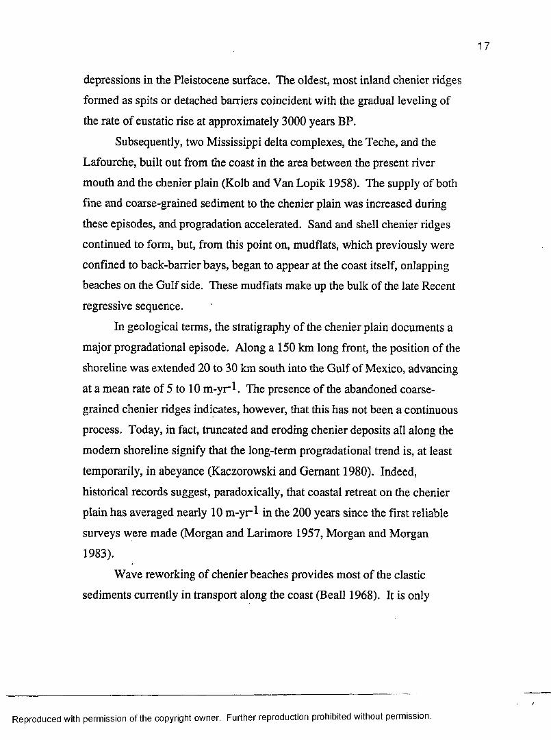
intersecting the coast for at least 1.5 years (Fig. 8).
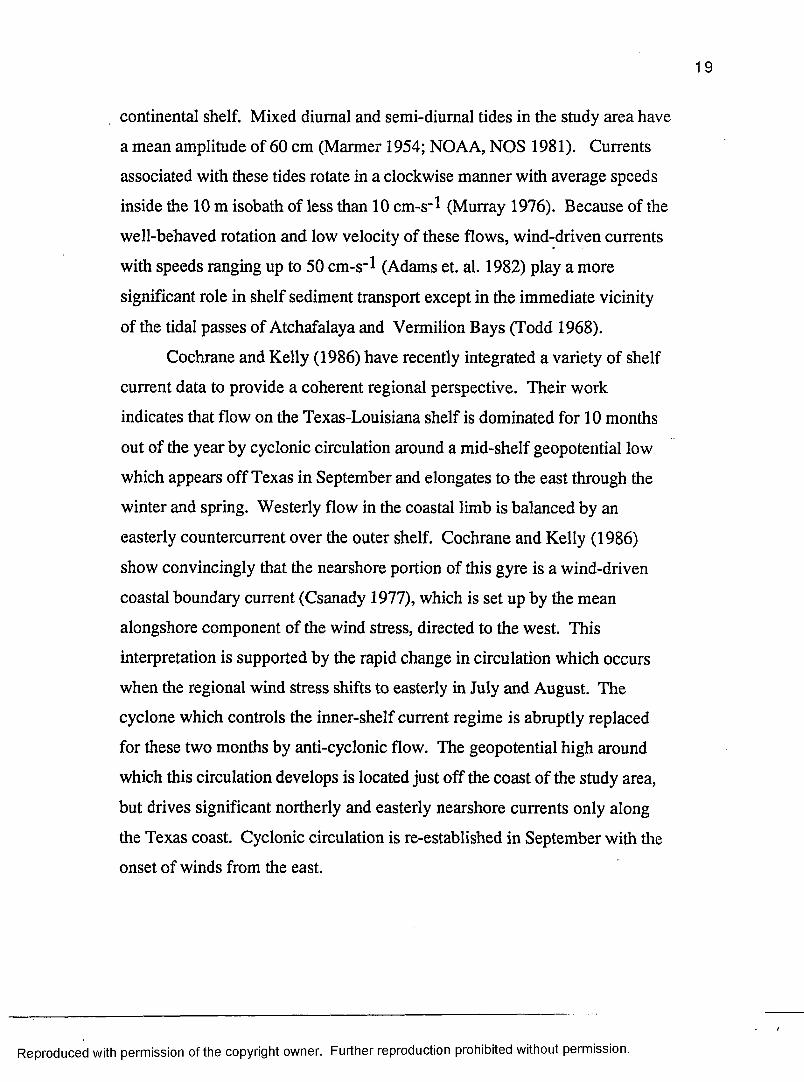
An elevated bar or berm on the seaward margin of the mudflat is
typical of new deposits (Fig. 9) of highly fluid sediment (Fig. 10a).
Subsequently, the bar and other regularly exposed areas dry and the surface
cracks into ever smaller polygons (Fig. 5a). When these areas are subject to
wave action, pieces of the surface crust are ripped up and the mudflat
acquires an irregular surface. The bar is usually gone by the beginning of the
winter following deposition (Fig. 9). Mud clasts, shells, and "coffee
grounds" accumulate in offshore-oriented erosional grooves or flutes (Fig.
10b). If new mud is deposited the next spring, that part of the mudflat which
survives the winter will be protected from further erosion. Oyster grass
(Spartina altemifloral then propagates onto this newly available land.
Freshly deposited mud is easily removed, and mudflats undergo
Reproduced with permission of the copyright owner. Further reproduction prohibited without permission.
/
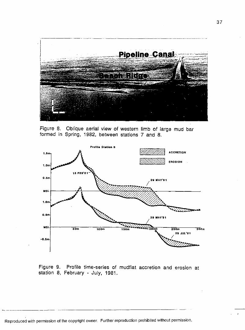
Figure 8. Oblique aerial view of western limb of large mud bar formed in Spring, 1982, between stations 7 and 8.
P r o l l la S ta t io n 8
ACCRETION1.5m -
EROSION1.0m
13 FEB’81
0.5m2 9 MAY’8 1
MSL
1.0m -
0 .5 m2 9 MAY’S 1
MSL 50 m 3 0 0 m1 0 0 m 2 5 0 m2 9 J U L '8 1
1 5 0 m
-0 .5 m
Figure 9. Profile time-series of mudflat accretion and erosion at station 8, February - July, 1981.
Reproduced with permission of the copyright owner. Further reproduction prohibited without permission.

38
r
Figure 10a-b. Shoreface mud at station 7; Freshly-deposited fluid mud, Spring 1982 (10a); eroding surface showing development of shore-normal flutes 5 months later (10b).
Reproduced with permission of the copyright owner. Further reproduction prohibited without permission.

39
erosion in all seasons. The most rapid retreat, however, occurs during the
summer immediately following a major depositional event (Table 1). Then,
the bar loses definition as sediments are redistributed both landward and
seaward along the profile section (Fig. 9). Progradation may more than
offset shoreline retreat in any given year, but the required sedimentation
does not occur at a uniform rate, or at the same locations each year. As a
result, zones experiencing major deposition in any single spring may be
separated by long stretches of shoreline which receive little or no mud. The
data summarized in Table 1 shows that between May, 1981, and May, 1982,
shoreline translation, whether through accretion or erosion, was far more
active at mudflat stations 6,7, and 8, than at any of the stations east of the
canal. The shoreline shifted 15 and 20 m seaward in this period at stations 6
and 7, respectively, but moved 33 m landward at station 8. It is illustrative of
the dynamic nature of the mud-fronted coast that between February and May,
1981, the months just prior to the two year period considered above, the
shoreline at station 8 moved seaward 108 m (Fig. 9).
A log of the 5.5 m vibracore from station 3 is provided in Figure 11.
Coring took place 20 m from the shoreline in the marsh which now covers a
mudflat described by Morgan et al. (1953). The core penetrated a
bioturbated sandy mud at 3.2 m below the marsh surface which matches
Coleman's (1966) description of nearshore marine sedimentation.
The upper 2 m o f the core record the mudflat and marsh sequence.
The basal 0.5 m of this sequence fines up and is composed of poorly-defined
layers of silty-sand and clayey-silt with no discernible erosion surfaces.
Radiographs of this section show wavy bedding distorted by water escape
structures (Fig. 12a) which may be artifacts of the coring process. In
Reproduced with permission of the copyright owner. Further reproduction prohibited without permission.
/

CHENIER AU TIGRE-CORE T 3
«SAND tSH E L L «ORG C LfTHOLOGV 0 SO 0 10 0 2
UNIT DESCRIPTION
wim Imbricated eJwie
2to lOcmttttoKbattocomooeedof lemmatad dbownoyrnaeaaamudiacwand M common at baaa of ootoata; btrrowa. roots, mud cracfca, and concisions tHupaauaon: •hall haen and aand present atbaaa ofutt ;iarmnationa change from oonvaua and tontiojnr naar oaaa to wavy and flat hmg farther up; Aama and toed svucaras convnon naar Oaaa
dean aand and anal; tomnaoona ndacrrt btf no burrows teoma wavy iamrae andamel- seals i-baddtoq; tnoncatedshalel baaa
Intaroaddad aand end mud;wedge-shaped poorty-aonedlaminattons; shelt-noah at baaa; no burrowa
heevfy bisrowed. faw tontteufar and wavy aand/attt laminae dUcernaols ; aftail haan secumuettone{burrowingrHenwty Ineraaaaa witti depth
DEPOSmONALENVIRONMENT
BEACH/M ARSH
MUDFLAT
BAR
TR A N SITIO N A L
(BAR TROUGH)
N EA R SH O R EMARINE
Figure 11. Log of vibracore from marsh now covering mudflat described by Morgan et al. (1953) west of Cheniere au Tigre at station 3; see Figure 6a-b.
Reproduced with permission of the copyright owner. Further reproduction prohibited without permission.

contrast, bedding is well-preserved in the overlying sand-free mudflat
sediments and shows repeated 2 to 10 cm thick beds consisting of flat and
lenticular silt laminae overlain conformably by a layer of featureless silty-
clay. The clay layer makes up an estimated 60 to 90 percent of the thickness
of each couplet. Erosional surfaces separating the couplets are marked by
scour-and-fill structures (Fig. 12b), and, in some cases, by thin layers of
imbricated Mulinea shells (Fig. 12c). Five of these cycles were recognized
below the bioturbated, organic carbon-rich marsh horizon. A 0.2 m thick
cross-bedded sand and shell washover deposit caps the rooted zone.
Mineralogy and Rheologv
The cyclic bedding observed in the upper mudflat section of the
vibracore produces variations in bulk density with depth. Overall, the trend
in a push-core obtained through newly deposited mud is from 1.2 g-cm-3 at
the surface to 1.4 g-cm-3 a meter below (Fig. 13). The density increase
occurs as a series of steps, however, increasing downward within each silt-
mud or shell-mud couplet to the point where grain-size data indicates the base
of the cycle. Bulk density drops off abruptly below the erosional interfaces
so that the upper part of each cycle is underconsolidated. The percent of
sand-sized particles (mainly shell) in the mudflat samples from this core
ranged from near zero to 14 percent. Silt content varied between 20 and 50
percent, while clay made up the remainder, between 50 and 80 percent of the
total. The within-bed pattern of consolidation, apart from the trend which
characterizes the deposit as a whole, suggests that each of these couplets
represents sedimentation occuring during a single depositional event.
X-ray diffraction traces from the <1 micron fraction of mudflat
sediments subjected to the standard suite of laboratory treatments are shown
Reproduced with permission of the copyright owner. Further reproduction prohibited without permission.

Reproduced
with perm
ission of the
copyright ow
ner. Further
reproduction prohibited
without
permission.
Figures 12a-c. Bedding structure in radiograph positives of mudflat sequences
(light tones indicate higher density silt and shell); flat and lenticular
laminae distorted by loading and water escape (12a), flat-lying silt
laminae filling scour depressions in underlying erosional surface (12b),
lamina of disarticulated, imbricated M ulinea valves at erosional surface (12c).

43
C O A R S EF R A C T I O N
(% > 63 M) D E P T H
D E N S I T Y(g -c m " 3)
30
50
70
90
Figure 13. Texture and bulk density changes with depth in upper meter of newly deposited mudflat.
Reproduced with permission of the copyright owner. Further reproduction prohibited without permission./

44
in Figure 14. The major clay mineral groups identified were illite, smectite,
and kaolinite. As is shown in Table 2, the two analytical methods used to
obtain semi-quantitative estimates of the abundances of these minerals give
somewhat different results for the dominant expanding-lattice illite and
smectite groups.
The method of Griffin (1971) is similar to techniques which have been
used in previous studies of sediments in Atchafalaya Bay and the inner shelf
(Powers 1957, Johns and Grim 1958, Whitehurst et al. 1960, Ho and
Coleman 1969, Brooks 1970, Mobbs 1981, Van Heerden 1983). Mobbs
(1981) worked both in the Bay and just offshore, and found insignificant
differences in composition between the two locations. Comparing his results
with earlier work, he did, however, suggest a long-term trend toward an
increased illite fraction in the most recent deltaic sediments. Van Heerden
(1983) noted a similar trend in cores containing both bay bottom sediments
and those associated with the newly emergent subaerial delta. He further
observed some indication of an increased illite content in flood deposition
relative to low-flow sedimentation. Mean percentages for the < 2 micron
fraction from Mobbs (1981) are presented in Table 2, and show a somewhat
higher percentage of illite relative to smectite than do the comparable
mudflat results.
A mixed-layer illite-smectite group was identified in the mudflat
sediment using the more detailed method of Schultz (1964). This mixed-
layer clay makes up almost half of the smectite identified following Griffin
(1971). This mineral group can form when degraded illite enters seawater
and regains much of its original potassium content (Johns and Grim 1958).
The dominance of the transitional mixed-layer illite-smectite clay in
Reproduced with permission of the copyright owner. Further reproduction prohibited without permission.
/

45
A IR -D RI ED
GLYCOLATED
3 3 0
5 5 0
10 15DIFFRACTION ANGLE (29 )
2520 3 0ANGLE
Figure 14. X-ray diffractograms of smears from the < 1ji fraction of mudflat sediments treated as indicated: S=Smectite, l=lllite,K=Kaolinite, and Q=Quartz.
Reproduced with permission of the copyright owner. Further reproduction prohibited without permission.
/

46
Table 2 Clay Mineral Abundances
Chenier Plain Mudflat and Atchafalaya Bay
Clay Mineral Atchafalaya Bay <2 jim
Kao Unite
Il l i te
Sm ectite
M ixed-LayerIllite -S m e c tite
%Mobbs (1981)
16d)
53
31
Chenier Plain <1jim
Methods--------Griffin(1971) Schultz(1964)
— % ..............17 19
%
43
39
31
20
30
(^Includes Chlorite
Reproduced with permission of the copyright owner. Further reproduction prohibited without permission.

47
sediments from the study area suggests a close connection between mudflat
deposition and the illite-rich Atchafalaya suspended load.
Results of viscometer runs on newly deposited mudflat sediment with a
bulk density of 1.26 g-cm-3 (sediment concentration = 416 g-l_l) and a
salinity of 22 °/OQ are summarized in the shear stress - strain rate plot in
Figure 15. The data describe an approximately linear relationship (r2 =
0.93) between the applied shear stress, T, and the rate o f deformation, du/dy.
The equation for this line describes the behavior of a Bingham plastic
T = T p + |i (du/dy) (1)
where Tp is the shear stress corresponding to the yield strength, and |i is the
sediment viscosity (Bingham 1922). Deformation ceases when the applied
shear stress falls below the yield strength. The yield strength, 171
dynes-cm"2, and viscosity of the mudflat sediment, 52 dyne-s-cm_2, are
determined by the intercept and slope, respectively, in Figure 15.
Krone's (1962) relationship between yield strength and sediment
concentration has the form
Tp = FC2.5 (2)
where C is the sediment concentration in g-1‘1, if Tp is measured in dynes-
cm-2. The experimental results indicate a value of 4.9 * 10"5 for the
proportionality factor, F. If Krone’s empirical relation holds, determination
of this factor allows estimation of yield strength for a range of sediment
concentrations. The line described by this equation is plotted on Figure 16
(adapted from McCave 1984) along with results for other marine muds
(Krone 1962,1963, Owen 1975, Hydraulic Research Station 1979).
Reproduced with permission of the copyright owner. Further reproduction prohibited without permission.

48
5 0 0 i
4 0 0
/* = 51.7dyne-s-cm-2
S t 3 0 0OC o < >
Z 2 0) >9 2 0 0
100 Tp = 1 7 0 .9 dynes-cm -2
0 1 32 4s-1
DEFORMATION RATE(du/dy)
Figure 15. Shear stress-strain rate plot from capillary viscometer measurements made at 22° C on mudflat sediment with a density of 1.26 g -cnr3 (sediment conc. = 416 g-M ), and a pore water salinity of 22 °/00. Bingham plastic behavior is indicated by the presence of
a Bingham yield strength, T p , of 170.9 dynes-crrr2
Reproduced with permission of the copyright owner. Further reproduction prohibited without permission.

49
1 0 0 0 .0
C9 1 0 0 .0
1.0
"S .
0.440 60 1002 0 2 0 0 40010
SEDIMENT CONCENTRATION (g-l-1 )
Figure 16. Fluid mud yield strength plotted as a function of sediment concentration (from McCave 1984). Data from Krone (1963), Owen (1970), and Hydraulics Research Station (1979) for a variety of marine muds plot with approximately the same trend (T p = F C 2-5). This trend is extrapolated from the mudflat data along
the dashed line shown.
Reproduced with permission of the copyright owner. Further reproduction prohibited without permission.
/

50
DYNAMICS EXPERIMENT
The wind record for 10 through 13, December, 1982, in Figure 17,
shows the 180° shift in direction which marks the passage of a cold front in
the early morning hours of the 1 l^h . Wave characteristics, flow velocities,
and suspended sediment concentrations were monitored in the three sessions
indicated.
The pre-frontal regime began at midday on the lO^1 with the onset of
easterlies ranging between 10 and 15 knots. The steady pre-frontal regime
lasted 15 hours and includes the period of the first two instrument runs.
Starting at midnight, wind direction rotated in a clockwise manner from
easterly to northwesterly during the next 8 hours. Speeds averaged less than
10 knots during this shift, which we identify as the frontal period. A rapid
increase in velocity after runs 3 through 6, on the afternoon on the 1l^ 1,
signaled the onset of the post-frontal regime. Northwesterly winds
strengthened over the next 8 hours to sustained speeds between 25 and 35
knots. Eight hours later, velocity dropped to between 15 and 25 knots, but
continued steady from the north throughout the 12^ . Wind azimuth then
shifted clockwise a second time in the early hours of the 1 3 ^ and speeds
dropped off to 10 to 15 knots. By midday, during the period of runs 7
through 10, winds were from the east once again.
The effects of front passage were manifested in departures of the
observed tide record from that predicted, in changes in the gravity wave
regime, and in the distribution of suspended sediments above the bed. These
effects are described in the first three sections below. The final results
section is focused on the relationship between infragravity water level
oscillations and low pass flow velocities.
Reproduced with permission of the copyright owner. Further reproduction prohibited without permission.
/

RUNS1 - 2
RUNS7-10100 PREDICTED
E3 50zO< MGL >UJmi
OBS ERVEDUJHI “50 O
\ - /
HZsN<
(0g 30Z*o 201UUJa(0a 10 z5
10 13
Figure 17. Winds and tides during cold front experiment, 1 0 - 1 3 December, 1982. Tide level recorded at the experiment site are compared with those predicted at the mouth of the Mermentau River (NOAA, NOS 1981). Wind data are hourly observations at Freshwater Bayou Canal Lock. The periods of the pre-frontal, frontal, and post- frontal instrument runs are indicated by stippling.
Reproduced with permission of the copyright owner. Further reproduction prohibited without permission.

52
Meteorological Influences on the Tide Record
W ater level at Freshwater Bayou Canal is plotted along with that
predicted at the mouth of the Mermantau River in Figure 17 (NOAA, NOS
1981). This gauging station, located 70 km west of the Canal, is the closest
for which predictions are made. Although the mean tide range there exceeds
that at Freshwater Bayou by 0.1 m, a general comparison can be made.
W ater level is an average of 0.2 m above predicted for the pre-frontal period
on the 10th Predicted and observed elevations are in agreement on the 11 &
coincident with front passage. Following the onset of the strong
northwesterlies later that day and continuing through the 12th, Freshwater
Bayou levels average 0.3 m below predicted. On the 13^ , the water level
depression was reversed as easterlies again set in.
Waves and Oscillatory Flow
Four kilometers offshore of station 6, significant wave height during
the first 6 data runs (Pre-frontal and frontal periods) was estimated at 1 m.
The wave field at this time included a long-crested swell which approached
the shoreline from the south-southeast at a 5 to 10 degree angle of incidence.
Following front passage, wave height offshore was less than 0.5 m, but a
short-crested, confused sea made the dominant direction of approach
impossible to assess.
Wave data acquired at the experiment site are summarized in Table 3.
W ater depth ranged from 85 to 105 cm, and wave heights averaged less than
20 cm. These low-amplitude waves formed spilling breakers at a point 30 m
landward of the instrument array during the first two runs (pre-frontal
period). In all subsequent runs, waves were completely attenuated before
reaching the shoreline, and breaking waves were not observed.
Reproduced with permission of the copyright owner. Further reproduction prohibited without permission.

Reproduced
with perm
ission of the
copyright ow
ner. Further
reproduction prohibited
without
permission.
Table 3Sea and Swell Wave Statistics
Cold Front Experiment 1 0 - 1 3 December, 1982
Run No. Time FlowmeterOrientation
W aterDepth
d(cm)
Period T (s)
Height ^rms (cm)
Wavelength L (cm)
Orbital Vel. Urms (cm-s-1)
Swell/Sea Swell/Sea Swell/Sea Swell/Sea
Pre-Frontal 12/10 2 14:20 On/Off 85 6.8 3.0 10.4 10.2 2097 965 17 18
Frontal 12/113 13:07 On/Off 100 6.9 2.8 11.3 4.4 2174 829 22 84 13:38 Along 100 7.3 3.5 11.0 4.6 2242 1107 — —
5 14:23 Along 100 5.8 3.5 13.0 4.3 1806 1107 — —
6 15:09 On/Off 90 6.1 3.2 8.9 3.6 2000 976 20 9
Post-Frontal 12/137 10:51 On/Off 85 6.5 2.8 5.6 6.3 2067 829 9 118 11:30 Along 90 8.0 3.2 5.3 5.7 2397 976 — —
9 12:34 Along 100 7.3 3.4 5.1 4.8 2290 1025 — —
10 13:01 On/Off 105 6.8 2.5 5.0 4.9 2097 761 8 8
Mean 96 6.8 3.1 8.4 5.4 2130 953 15 11Std. Dev. 8 0.7 0.4 3.1 1.9 173 123 6 4
cnco

54
The effects of front passage on wave height and oscillatory flow can be seen
in the sequence of pressure and flowmeter spectra shown in Figure 18.
Spectra computed from representative 20 minute pressure and flowmeter
records acquired before, during, and after front passage all show energy
density peaks at two frequencies in the gravity wave range. These peaks
define distinct wave trains; swell with an average period of 6.8 s (0.1471 cps)
and locally generated seas of 3.1 s period (0.3226 cps). The energy
contributed by linear trends and infragravity oscillations of period greater
than 200 s (0.005 cps), combine to form a third peak which appears close to
the origin in all the spectra. Root-mean-square wave heights (Hrmg) and
oscillatory flow velocities (Um s ) calculated for the principal gravity wave
peaks (Thompson 1981) are also included in Table 3.
Two changes in the wave field associated with the transition from pre-
to post-frontal conditions are apparent. First, the total gravity wave energy,
consisting of the combined contributions of both sea and swell, decreases
through the sequence. Second, the distribution of energy between swell and
sea frequencies shifts significantly. Hnns and UnxiS in both bands are of
comparable amplitude in the pre-frontal runs. Energy associated with the
swell is retained during the second sampling period coincident with the shift
to northwesterly winds, while that of the seas is greatly diminished. Finally,
a reduced, residual swell and building seas characterize the final, post-frontal
records.
The differences in inferred wave height between seaward (A) and
landward (B) pressure sensors 10 m apart were less than 5 percent in all runs
where simultaneous data were obtained. Although it was noted qualitatively
that, except during the pre-frontal period, waves were completely attenuated
Reproduced with permission of the copyright owner. Further reproduction prohibited without permission.
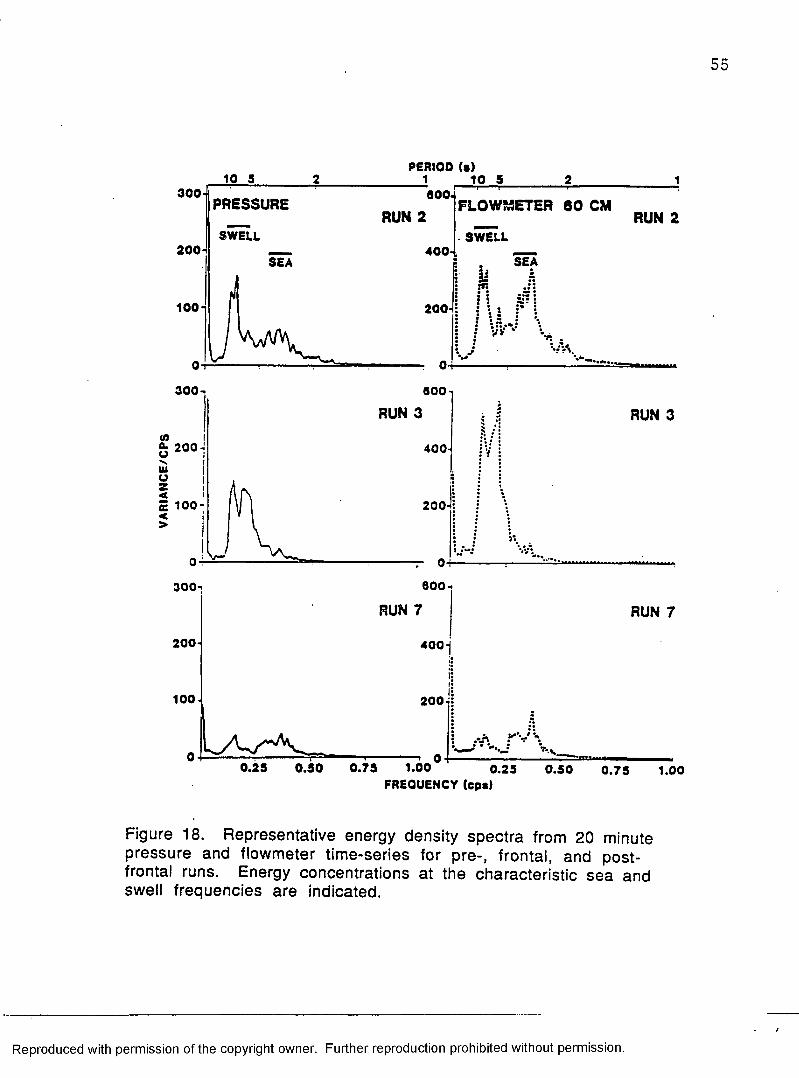
PERIOD (•)10 5
300 -IPRESSURE
SWELLSIa
FLOWMETER 6 0 CMRUN 2 RUN 2
■ SWELL200-I 400- SEA
100-1 200-1
3001 600
RUN 3 RUN 3
200 ■! 400-
200 -
600300-;
RUN 7 RUN 7
200 - 400 -j
1 0 0 - 200
0.25 1.00FREQUENCY (cps)
0.50 0.75 0.25 0.50 0.75 1.00
Figure 18. Representative energy density spectra from 20 minute pressure and flowmeter time-series for pre-, frontal, and post- frontal runs. Energy concentrations at the characteristic sea and swell frequencies are indicated.
Reproduced with permission of the copyright owner. Further reproduction prohibited without permission.

56
before reaching the shoreline, comparison of water level spectra at the two
stations indicates that in four runs, wave height actually increased slightly in
the landward direction. Such an increase can be seen in spectra from run 3
plotted in Figure 19a.
Coherence and phase estimates computed from the cross-spectra of
simultaneous water level records from run 3 are also shown in Figure 19a.
The relationships between coherence, phase, and frequency shown in this
figure are representative of all the runs and provide information about the
incident waves which cannot be deduced from individual spectra. As is
expected, coherence between the records is highly significant through all
frequencies with appreciable energy. The strength of the correlation lends
credibility to the phase trend shown.
Below 0.005 cps, in the infragravity peak, the two records are in
phase. The gradual increase in lag with increasing frequency suggests that
the spectral peaks observed in the gravity wave range are associated with
progressive waves rather than standing waves or spectral harmonics
(Suhayda 1974). Given that the spacing between the sensors is known
exactly, the magnitude of the phase lag at the principal gravity wave
frequencies provides a direct measure of swell and sea wavelengths. Mean
wavelengths of the swell and sea calculated in this way were 21.3 m and 9.5
m, respectively (Table 3).
Spectra of flowmeter records obtained at 60 and 13 cm above the bed
during the same run are shown in Figure 19b. Energy densities at swell
frequency during this run were somewhat higher at 13 cm than at 60 cm, but
in most onshore-offshore runs, gravity wave energy was almost identical at
all levels. Coherence and phase estimates from the cross-spectra indicate that
Reproduced with permission of the copyright owner. Further reproduction prohibited without permission.
/

10 sPERIOD (a )1 10 5
3 0 0 -l
O 2 0 0 -MlU
100
PRESSURE: RUN 3 ••a w a rd sanaor (A)
•horaw ard sanaor (B)
600
AOf
• VV
400
200i
i ife c J
FLOWMETERS: RUN 3* . . . . . 6 0 cm
— 13 cm
■ <»Jo-f v
1-0-1 1.0-1
ttluziusUlzoo
0.5-0 .5 -
i 0 . 0 -
(B) lags (A)
0.250.75 0.50 0.750.25 0.50 1.00FREQUENCY ( c p a )
Figures 19a-b. Concurrent spectra, and cross-spectral estimates of coherence and phase for records from run 3; between seaward and landward pressure sensors located 10 m apart (19a), and between near-surface and near-bottom flowmeters (19b).
Reproduced with permission of the copyright owner. Further reproduction prohibited without permission.

58
oscillatory flow at the two elevations is highly coherent and in phase. These
observations suggest that oscillatory wave motion is reasonably
approximated by potential flow, at least down to 13 cm above the bed
(Komar 1976, p. 39).
A knowledge of wave height, water depth, and wavelength is sufficient
to classify surface gravity waves within the bounds o f specific wave theories.
As is shown in Figure 20, adapted from Komar (1976, p. 61), both sea and
swell fall within the range of Airy or Linear Wave Theory (LWT), well
below the line beyond which wave steepness is limited by breaking. Because
of their limited wavelength, the seas are considered "intermediate water"
waves even in 1 m water depth and lie outside the region where LWT shallow
water approximations are most valid.
Wavelengths determined from the cross-spectra average 6 percent
longer than those calculated using shallow water LWT, as is indicated by a
slope slightly less than unity in Figure 21a, but otherwise are well predicted
by this theory (r2 = 0.92). The oscillatory velocity data plotted in Figure 21b
also shows a good fit (r2=0.99) between Urms determined from spectra, and
the theoretical maxima predicted. Umax exceeds Unns, as is expected. The
62 percent difference is, however, an indication that orbital velocities
calculated from the spectra provide a somewhat inadequate representation of
oscillatory flow for the shoaling waves considered here (Cornish 1898). In
all runs, at all depths, an assymetry was observed between maximum onshore
and offshore velocities, both before and after correction for the low-
frequency mean flow component. Corrected peak onshore orbital velocities
exceeded offshore maxima by an average of 28 percent.
Reproduced with permission of the copyright owner. Further reproduction prohibited without permission.

Lina of l imiting w i v « s t a a p n a s a
£ ' / S W E L L > v EA
H /d 0.1
AIRY WAVE THEORY
Airyd e e pw a t e r
Airy Airy’■N
sha l l ow 'o i n t e r m e d i a t e w a t e r w a t e r
0 .010 .01 0.1 1 10
Figure 20. The areas of application of the several wave theories as a function of H/d and d/L (from Komar 1976, p. 61). The regions occupied, within the span of Airy or Linear W ave Theory (LWT), by seas and swell monitored during the cold front experiment are shown in stippling.
Reproduced with permission of the copyright owner. Further reproduction prohibited without permission.

60
(A)2 2
*y = 0 . 9 1 x ♦ 0 . 5 7
140 . 9 2
10
6 1 0 1 4 18 2 2 2 6WAVELENGTH FROM CROSS-SPECTRA (m)
Q
(B)
« 3 0
y = 1 . 6 1x ♦ 0 . 1 7
2 2 0 . 9 9
1 4 2 2 3 0
Urms FROM SPECTRA (cm -*’ 1 )
3 8 4 6
x<2
Figures 21a-b. Relationships between wave parameters determined from the spectra and cross-spectra, and those predicted by shallow water LWT; wavelength (21a), and orbital velocity (21b).
Reproduced with permission of the copyright owner. Further reproduction prohibited without permission.

61
Suspended Sediments
Total suspended sediment concentration results from the multi-level
sampler are summarized for the pre-frontal, frontal, and post-frontal
periods in Table 4. Concentrations ranged from 160 to 9400 mg-l“l. Both
concentration and between-sample variability decreased with elevation above
the bed. The highest concentrations, which approached those of fluid mud,
were monitored at 10 cm above the bed during the frontal period (runs 3 - 6 ) .
Concentrations at this elevation, during these runs, averaged more than 10
times greater than during the pre-frontal period, and 3 times higher than the
post-frontal mean.
Ratios calculated between concentrations at the 65 and 10 cm levels are
shown in Table 4. Near-bottom concentrations (10 cm elevation) during the
frontal period were 550 percent higher than at 65 cm, but only 2 and 54
percent greater during the pre- and post-frontal periods, respectively. These
results indicate that a significant vertical gradient in sediment concentration
was developed in the frontal runs which was not present during the other two
periods. Representative concentration profiles from runs 2, 3, 5, and 7,
plotted in Figure 22, show the progression of gradient development through
the frontal sequence.
It is clear that suspended sediment concentrations are not directly
related to wave energy as the highest values near the water surface were
found during the post-frontal period when wave heights were lowest. One
interpretation of the distinctive character of the frontal profiles, relative to
those from the pre- and post-frontal periods, is that gradient development
may be linked to the frequency composition of the gravity wave energy,
rather than to wave amplitude. Ratios of sea to swell wave
Reproduced with permission of the copyright owner. Further reproduction prohibited without permission.
/

Reproduced
with perm
ission of the
copyright ow
ner. Further
reproduction prohibited
without
permission.
Table 4 Total Suspended Sediment
Cold Front Experiment 1 0 - 1 3 December, 1982
Run No. Time Water No. Height Ratio Mean Cone. (Std. Dev.) Cone. Ratiodepth Samples Sea/Swell sampled at 4 elev. 65cm/10cm
d (cm) 95 cm 65 cm 35 cm 10 cm....................... - m g - h 1 - - ..................................................Pre-Frontal 12/10
2 14:20 85 4 0.98 — 318( 53) 320( 45) 325( 56) 0.98(.03)Pre-Frontal Mean 4 0.98 — 318( 53) 320( 45) 325( 56) 0.98(.03)
Frontal 12/113 13:07 100 3 0.39 205(28) 256( 92) 350( 61) 3213(3531) 0.13(.07)4 13:38 100 2 0.42 304(21) 355( 4) 634(232) 4650(2792) 0.09(.06)5 14:23 100 3 0.33 360(54) 341 ( 25) 362( 11) 5666(3597) 0.09(.06)6 15:09 90 3 0.40 337( 95) 515(129) 1155( 358) 0.30(.09)
Frontal Mean 11 0.39(.04) 290(99) 317( 76) 443(152) 3582(3037) 0.16(.11)
Post-Frontal 12/137 10:51 85 6 1.12 820( 61) 901 ( 82) 1355( 398) 0.66(.21)8 11:30 90 6 1.08 582( 46) 618( 86) 1131(455) 0.61 (.28)9 12:34 100 6 0.94 413(12) 426( 16) 439( 29) 732( 250) 0.65(.23)
10 13:01 105 6 0.98 431(20) 477( 20) 466( 18) 773( 391) 0.69(.27)Post-Frontal Mean 24 1.03(.08) 425(19) 568(168) 606(196) 998( 443) 0.65(.23)
Grand Mean 96 39 0.74(.34) 364(93) 473(185) 533(200) 1658(2020) 0.54(.33)
CDro

100
5 0
Eo
aUi“ 10 iu > o m <
tTl fcml
RUN 2
— ,— imu
RUN 3
* Vinmi~lQmi|lmjni|i
RUN 5-i 50RUN 7
J ,li minmfan'lilfl.nnmri101000 10000100
SUSPENDED SEDIMENT ( m g - f1)
Figure 22. Mean suspended sediment concentrations from representative pre-frontal (2), frontal (3 and 5), and post-frontal (7) runs. Error bars show two standard deviations about the mean.
Reproduced with permission of the copyright owner. Further reproduction prohibited without permission.

64
heights, given in Table 4, provide one measure of the relative importance of
these components of the wave field. When the near-surface/near-bottom
concentration ratios (65cm/10cm) from each run are plotted against the
respective wave height ratios, the data from the pre- and post-frontal periods
form one cluster distinctly separate from a second frontal cluster, as is shown
in Figure 23. The concentration ratios exhibit large within-run variability,
as is indicated by the error bars in the figure. Within-run variability in the
wave height ratios cannot be estimated. Even so, when all the data are
considered together, a weak linear relationship emerges (r2 = 0.69). This
result suggests that swell waves may contribute to the formation of a
suspended sediment gradient, which does not develop if higher frequency
seas make up an important part of the wave field.
Infragravitv W ater Level Changes and Non-Oscillatorv Flow
Energy contained in the low-frequency peak below 0.005 cps
constitutes between 30 and 60 percent of the total variance in the water level
data, and from 7 to 22 percent of that in onshore-offshore flowmeter
records. An average of 54 percent of the low-frequency variance in the
pressure records is contributed by uni-directional tidal trends in water level
which are long with respect to the 20 minute sample length. These can be
approximated by a straight line and are readily removed using a linear
detrending procedure. Non-tidal water level fluctuations contribute the
remaining low-frequency variance. As was noted earlier, concurrent water
level spectra obtained 10 m apart differ by less than 5 percent in the gravity
wave frequencies, and, overall, indicate no consistent cross-shore pattern
with respect to wave height. In contrast, a systematic amplitude increase in
the direction of the shoreline is observed below the gravity wave range. The
Reproduced with permission of the copyright owner. Further reproduction prohibited without permission.
/

o5 1 - °oczoj= 0.8<OCz Eg S 0 .6 -
siO o
IA <0
O*£<<>0.4UJ2Ew 0.2</>Q UJa zUJ CL CO
1.00 .2 0.4 0.6Hsea/Hswei!
1.20.8
WAVE TYPE RATIO
Figure 23. Relationship between vertical sediment concentration gradient, indicated by the ratio between near-surface and nearbottom values, and the relative significance of sea and swell, indicated by the ratio of their respective heights determined from the spectra. Circled numerals correspond to run number, and error bars indicate two standard deviations about the mean concentration ratio for each run.
Reproduced with permission of the copyright owner. Further reproduction prohibited without permission.

6 6
sum of variances in spectral frequency bands below 0.005 cps from the
detrended water level records are listed by station in Table 5.
Between-station differences provide a relative measure of the
landward amplification of the non-tidal, low-frequency water level changes
occurring during each run. This amplification was less than 5 percent in 2 of
the 7 runs from which data at both (A) and (B) are available, but ranged from
11 to 33 percent in the remainder, and averaged 12 percent overall.
Concurrent water level records are in phase at frequencies below 0.005 cps,
as the cross-spectral results in Figure 19a show for run 3. An amplitude
increase in the direction of the shoreline, without a progressive phase shift
over the same distance, is characteristic of a standing wave with an offshore
node and an antinode at the shoreline (Suhayda 1972, Waddell 1973).
Attention is drawn to the variance values for run 3 in Table 5 which
exceed the means for all runs by nearly 300 percent. Low-pass wave and
flowmeter data (T > 200 s) from run 3 are shown in Figure 24 and clearly
show the source of this energy. Mean water level drops gradually in the first
half of this segment, then abruptly rises 10 cm in 340 s. During this period of
rapid water level rise, flowmeters at all depths register significant onshore
flow. Most of the low-frequency adjustment in flow velocities occurs away
from the bed at the upper flowmeter elevations. The records shown in
Figure 24 clearly establish that coherent onshore-offshore flows lasting for
minutes are associated with non-tidal fluctuations in nearshore water
elevation. Local and regional wind data of comparable resolution are
lacking. It appears, however, that the wind-forced sequential water level set
up and set-down which characterizes the frontal tide record is reflected in
higher-frequency changes observed in 20 minute records.
Reproduced with permission of the copyright owner. Further reproduction prohibited without permission.

Table 5Water Level Variance Below 0.005 cps
in Concurrent Detrended Records from Stations A and B10 m Apart
Run Variance (cm)2 D ifference %No. --------------------
Station A Station B
P re -fro n ta l2 1.59 1.78 +0.19 + 12
Frontal3 7.74 8.63 +0.86 + 11
4 1.18 1.21 +0.03 + 3
5 1.54 1.71 +0.17 + 11
6 1.20 1.21 +0.01 + 1
P o st-fro n ta l7 0.87 1.16 +0.29 + 33
8 1.02 1.14 +0.12 + 11
Mean Std. Dev.
2.162.47
2.412.76
+0.240.29
+ 12 10
Reproduced with permission of the copyright owner. Further reproduction prohibited without permission.

Reproduced
with perm
ission of the
copyright ow
ner. Further
reproduction prohibited
without
permission.
RUN 3 LOW PASS
60cmT "O N S H O R E
IEo sr- 30cma111IIIQ.0)
1 3cmO F F S H O R E
300 1050750 900600 TIME (s)
450150
F igure 2 4 . Low freq u en cy w a ter le v e l and o n sh o r e -o ffsh o r e flow m eter d a ta from frontal run 3 . Low p a s s w ater le v e l is su p e r p o s e d on d e m e a n e d p r e ssu r e record in upper fram e. Low p a s s flow m eter v e lo c it ie s ab o u t a true z e r o point a re sh o w n in th e low er fram e. Logarithm ic flow p er io d s stip p led .
O)00

69
The existence of a connection between infragravity water level
changes and cross-shore flow is supported by analysis of the flowmeter
variance statistics presented in Table 6. Flowmeter variance less than 0.005
cps increases with elevation above the bed. Covariances were computed
between the low-frequency velocity time-series and the low-pass water level
records. Then the same comparison was made between the velocity data and
the time-series which results from evaluating the change in water level
between each time step. This simple derivative of the low-pass water level
time-series exhibits positive values when water level rises, and negative
values when it falls.
Change in the rate of water level rise and fall, represented by the
derivative time-series, is positively correlated with the low-frequency
flowmeter records and explains, on average, 60 percent of the variance in
velocity below 0.005 cps. The undifferentiated water level record explains
only 22 percent of the low-frequency onshore-offshore flow. The poor
correlation between untreated water level and velocity is not unexpected
given that maxima and minima in water level represent end points which are
out of phase with cross-shore flow. Physically, as the surface elevation
fluctuates about a mean position, high and low water stands are both periods
of diminished shore-normal transport.
The covariance data in Table 6 indicates that the correlation between
the rate of water level change (derivative) and shore-normal velocity is far
stronger at the 60 and 30 cm levels than it is closer to the bed, at the 13 cm
level. The reason for the decreased correlation there can be seen in Figure
25. This figure shows a progression of velocity profiles extracted at 50 s
intervals during the low-frequency flow event shown in Figure 24 (run 3).
Reproduced with permission of the copyright owner. Further reproduction prohibited without permission.
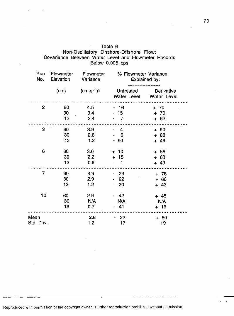
Table 6Non-Oscillatory Onshore-Offshore Flow:
Covariance Between Water Level and Flowmeter RecordsBelow 0.005 cps
Run Flowmeter Flowmeter % Flowmeter Variance No. Elevation Variance Explained by:
(cm) (cm-s-1 )2 Untreated Water Level
Derivative Water Level
2 60 4.5 - 16 + 7030 3.4 - 15 + 7013 2.4 - 7 + 62
3 60 3.9 - 4 + 9030 2.6 - 6 + 8813 1.2 - 60 + 49
6 60 3.0 + 10 + 5830 2.2 + 15 + 6313 0.9 - 1 + 49
7 60 3.9 - 29 + 7630 2.9 - 22 + 6613 1.2 - 20 + 43
10 60 2.9 - 42 + 4530 N/A N/A N/A13 0.7 - 41 + 19
Mean 2.6 - 22 + 60Std. Dev. 1.2 17 19
Reproduced with permission of the copyright owner. Further reproduction prohibited without permission.

Reproduced
with perm
ission of the
copyright ow
ner. Further
reproduction prohibited
without
permission.
80
708080
40
30
20ouoUl>oD<Zo
70I-<>111_]ui
60
6040
3020
T=675»10
-3 -2 1 0 21 43
O F F 8 H O R E O N S H O R E
T=575 8 T=626 s
1 30 1 42
V E L O C I T Y C C M - S - 1 )
!
Figure 25. Sequence of vertical velocity profiles from 525 to 775 s during onshore-offshore flow event in run 3 (see Fig. 24).
72
The sequence demonstrates that both onshore and offshore transport begin as
flow reversals close to the bed. This observation lends credibility to the
standing wave concept introduced earlier, as near-bottom flow reversals are
characteristic of transport predicted under both standing (Longuet-Higgins
1953) and partially reflected progressive waves (Carter et al. 1973). The 20
minute length of the records obtained during this study does not permit
resolution of the periodicity of the low-frequency water level fluctuations
observed, if, indeed, any such periodicity exists. Establishment of periodic
forcing is not required with respect to the kinematics, however, as any
perturbation of the free surface will involve a redistribution of mass
requiring shore-normal currents. These currents emulate those developed
under a true standing wave characterized by a particular node position and
frequency.
Spectra from flowmeters oriented alongshore have a significant peak
only at frequencies below 0.005 cps as the ducts eliminated an estimated 95
percent of the gravity wave signal. Alongshore flowmeter statistics compiled
in Table 7 lead to three important observations. First, alongshore flow was
to the west throughout the course of the experiment. Second, mean velocities
remained relatively constant, ranging from 7.6 to 8.1 cm-s"l at the 60 cm
elevation, through the frontal and post-frontal sequence when wave heights
dropped significantly. Finally, mean flow velocities in all runs increase with
elevation above the bed.
Low-pass wave and flowmeter data from run 5 are shown in Figure
26. The dependence of velocity on flowmeter elevation is more pronounced
in this alongshore data than in the onshore-offshore record from the same
period (Fig. 24). W ater level drops through most of this segment but rises
Reproduced with permission of the copyright owner. Further reproduction prohibited without permission.
/

73
Table 7 Steady Alongshore Flow:
Covariance Between Water Level and Flowmeter RecordsBelow 0.005 cps
Run Flowmeter Mean % Flowmeter VarianceNo. Elevation Westward Explained by:
Velocity ......................................(cm) (cm-s-1) - Untreated
Water LevelDerivative
Water Level
4 60 7.8 + 52 + 1130 4.5 + 49 + 1013 1.7 + 56 + 11
5 60 7.9 + 57 + 3530 5.6 + 66 + 4013 1.3 + 81 + 24
8 60 8.1 + 54 + 2030 6.2 + 48 + 1013 3.0 + 40 + 3
9 60 6.0 + 86 - 1630 N/A N/A N/A13 1.7 + 82 + 24
Mean 4.9 + 61 + 19Std. Dev. 2.6 16 11
Reproduced with permission of the copyright owner. Further reproduction prohibited without permission.

Reproduced
with perm
ission of the
copyright ow
ner. Further
reproduction prohibited
without
permission.
RUN 5 LOW PASS
30cm
n. ■-w o -----------------------------1-----------------------------1-----------------------------1-----------------------------1-----------------------------1---------------------------- 1-----------------------------1-----------------------------1-----------------------------< ■ ■■ i wISO 300 450 600 750 900 1050
TIME (s)Figure 26. Low frequency water level and alongshore flowmeter data from frontal run 5. Low pass water level is superposed on demeaned pressure record in upper frame. Westerly low pass flowmeter velocities about a true zero point are shown in the lower frame. Logarithmic flow periods indicated by stippling.
■vl

75
toward the end. Flowmeter velocities generally mirror the water level
curve, decreasing when water level falls, and increasing when water level
rises. As before, covariances were computed first between the low-
frequency flowmeter time-series and the untreated water elevation record,
and then between the velocity data and the derivative water level time-series.
For the alongshore runs, the untreated water elevation data is positively
correlated with velocity (positive to the west) and explains an average of 61
percent of the low-frequency flow variance. The derivative of the water
level time-series explains, on average, only 19 percent of the flowmeter
variance below 0.005 cps. Physically, the positive correlation between
alongshore flow velocity and water level means that maximum and minimum
velocities occur at high and low water stands, respectively. A rise in water
level, then, results in an increase in westerly alongshore flow velocities at the
instrument array.
The depth dependence of the mean alongshore velocities in Table 7
suggests that the alongshore current might be well characterized as a
boundary shear flow. The physical constraint that velocities must be zero at
the bed gives rise in a neutrally stable flow to a boundary modified layer in
which mean steady horizontal velocities typically approach free-stream
values as a logarithmic function of elevation above the bed (Adams and
Weatherly 1981a). The equation which expresses the relationship of
horizontal velocity to depth in the bottom boundary layer has the form,
u* zU = — In — (3)
K zo
Reproduced with permission of the copyright owner. Further reproduction prohibited without permission.
/

76
where U is the velocity measured at a reference height z above the bed and K
is von Karman's constant (0.4). This profile is fitted to the data by
minimizing the square of the velocity deviations with respect to a characteristic shear velocity, u*, and an apparent bottom roughness length,
z0 (Wilkinson 1984).
In the present investigation, low-pass velocities averaged over 5 s
intervals at each of the three flowmeter elevations were fit to equation (3) to obtain 240 profiles, with associated estimates of u* and z0, for each 20
minute record. A profile was defined as logarithmic when A , the coefficient
of determination, exceeded 0.9755, the t-test criterion for a 90 percent
confidence level in a three point fit (Adams et al. 1982). Low-frequency
onshore-offshore flows met this test between 5 and 25 percent of the time.
Alongshore flow, in contrast, was logarithmic for 65 to 85 percent of the
runs where three point velocity data was available (runs 4, 5, and 8), and was
close to logarithmic most of the rest of the time. Periods of significant
logarithmic flow are shown in the onshore-offshore record in Figure 24 and
in the alongshore data in Figure 26.
A subsample of velocity profiles meeting the logarithmicity test was
selected from periods of steady flow when the mean current was undergoing
neither acceleration or deceleration. It is important to note here, for
consideration later, that no periods of steady flow were found in the onshore-
offshore data. Ten steady flow profiles with r^ values above 0.99 were
identified, however, in each of alongshore runs 4, 5, and 8. Mean values of
u*, z0, and the velocities at each reference elevation derived from these
subsamples are given in Table 8 and were used to generate characteristic
steady flow profiles for each of these runs.
Reproduced with permission of the copyright owner. Further reproduction prohibited without permission.
/

77
The characteristic velocity profiles are shown in Figure 27. In these semi-log plots the y-intercept corresponds to z0, the apparent bed roughness,
while the slope is K/u*. The profiles for runs 4 and 5, which were obtained
less than 1 hour apart, are similar, while that from run 8 in the post-frontal
period differs significantly. At 60 cm, velocities in runs 4 and 5 exceed that
for run 8, while at 30 and 13 cm the reverse is true. Values for z0 in all of
these profiles suggest the presence of bottom roughness elements 2 to 5 times
the amplitude of any actually found on the smooth mud bed at the experiment
site (2 cm maximum).
In briefly reviewing the results of the cold front experiment, we note
that both sea and swell waves at the study site were well described by shallow
water LWT. The major effect of front passage on the wave field appears to
be a modulation of the relative importance of the high-frequency sea
component. A significant vertical gradient in suspended sediment
concentration was developed during the frontal period under essentially
monochromatic swell waves (runs 3 - 6). This gradient was not present
during the pre- or post-frontal runs, when seas contributed more
significantly to the spectral energy distribution. W ater level oscillations in
the infragravity region were observed to be correlated with unsteady cross
shore flows. The low pass alongshore current, in contrast, was found to be a
fully developed, and relatively steady, boundary shear flow.
Reproduced with permission of the copyright owner. Further reproduction prohibited without permission.

78
Table 8Characteristic Alongshore Velocity Profile Parameters
Run Tim e Water u* z0 Velocity %— at— Log
No. Depth 60cm 30cm 13cm.(cm) (cm-s-1) (cm) (cm-s-1)
Frontal Period 12/114 13:38 100 1.9 10.1 8.3 5.0 1.2 85
5 14:23 100 1.8 10.1 8.0 4.8 1.1 65
Post-Frontal Period 12/138 12:34 85 1.2 5.1 7.4 5.3 2.8 80
Reproduced with permission of the copyright owner. Further reproduction prohibited without permission.
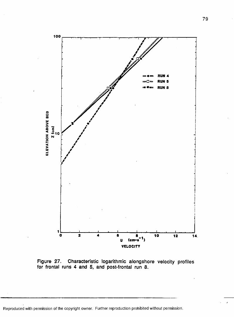
79
100
— RUN 4in O m RUN 5
r u n 3
aUJaUJ>Oa<zo<>UJmlUJ
0 2 4 0 8 10 12 14.1
VELOCITY
Figure 27. Characteristic logarithmic alongshore velocity profiles for frontal runs 4 and 5, and post-frontal run 8.
Reproduced with permission of the copyright owner. Further reproduction prohibited without permission.

D ISC U SSIO N
The results o f this study show that mudflat deposition has ceased east of
Freshwater Bayou Canal, but remains active in the western half of the study
area. Mudflats form there only in late winter and early spring, and are
characterized in cross-section by distinctive 2 to 10 cm thick beds displaying
both grading and flat-lying basal silt or shell laminae. The goal of
monitoring nearshore dynamics over a broad range of wave energy
conditions was achieved during the December cold front experiment. Fine
grained sediments were in motion during this event, but sequential bed
profiles conducted in the course of the experiment showed no significant
changes indicative of accretion or erosion. A conspicuous lack of
sedimentation is not surprising given the intermittency which characterizes
mud deposition in this area. It is, however, an important indication that all
factors necessary for nearshore mud deposition were not present at the time
of the experiment.
Significant water level set-up and set-down were associated with the
characteristic clockwise rotation in wind direction which accompanies front
passage. These effects were clearly manifested in departures from the
predicted tide, but also showed up as infragravity oscillations in 20 minute
nearshore water level records. These oscillations exhibited characteristics of
a standing wave with an antinode at the shoreline. Significant low-frequency,
onshore-offshore flows were correlated with these shore-amplified water
level changes and support an assumption of standing wave motion.
The sea and swell waves monitored during the cold front experiment
were found to be well described by shallow water linear wave theory, but
80
Reproduced with permission of the copyright owner. Further reproduction prohibited without permission.

81
also experienced the nearshore attenuation documented by Wells and
Coleman (1981a, b) on the muddy coast of Surinam. A significant near
bottom gradient in suspended sediment concentration was observed under
monochromatic swell waves, at the time of front passage, which was absent
when higher-frequency seas contributed significantly to the total wave
energy. Mean alongshore velocities near the surface responded to low-
frequency changes in the depth of flow at the flowmeter array, rather than to
changes observed in the incident wave field. This current consistently set to
the west in spite of the sequential shifts in wind direction which characterized
the cold front progression.
The vertical velocity distribution of the alongshore current, unlike that
of the the low-frequency shore-normal transport, was indicative of a steady,
logarithmic boundary shear flow. Apparent bottom roughness estimates (z0)
were, however, 2 to 5 times greater than the amplitude of any physical
roughness elements present at the experiment site. A marked decrease in both apparent bottom roughness, and the characteristic shear velocity (u*),
was noted in the transition between frontal and post-frontal profiles.
Now that we have some information about the nearshore dynamics, it
is appropriate to re-examine in more detail the boundary layer sorting model
(B-L-S model) proposed by Stow and Bowen (1980). Their representation
of the near-bottom dynamical environment is reproduced in Figure 28. Stow
and Bowen (1980) inferred, on the basis of sedimentological data alone, that
the origin of graded and laminated silt + mud beds must depend on a
fundamental difference in the way suspended cohesive and non-cohesive
sediments respond to boundary layer shear. Differential settlement of these
two types of particles in a waning flow could not explain the within-bed
Reproduced with permission of the copyright owner. Further reproduction prohibited without permission

SEA SURFACE
— z = h
TURBIDITYCURRENT
SUSPENSION
Nl
SHEAR
BOUNDARYLAYER10-
>VISCOUS SUB- { \ LAYERlam inarSUB-LAYER
SETTLING
Figure 28. B-L-S model for sorting of cohesive and non-cohesive sediments in the boundary layer of a turbidity current (from Stow and Bowen 1980). Elevation, z, measured from the bed in a millimeter logarithmic scale.
Reproduced with permission of the copyright owner. Further reproduction prohibited without permission.

83
sorting they found in fine-grained, shelf margin turbidite sedimentation, as
clay floes and silt grains with equivalent settling velocities would be expected
to deposit together. According to the B-L-S model, initially only silt grains
can settle through the high-shear zone to form the characteristic basal
laminae, while clay floes approaching the bottom are disaggregated and
returned to the flow interior. Stow and Bowen (1980) suggest that clay
concentrations build up above the boundary shear layer to the point that
aggregates form which are sufficiently large to "overcome" shear. At some
critical concentration, they penetrate the high shear zone, "break-up", and
deposit rapidly to form the characteristic mud "blanket" overlying the silt
laminae. Following deposition of a silt + mud couplet, the process is repeated
at the new surface, such that a sequence of stacked laminated and graded beds
is developed.
Observations made during the course of the present study indicate that
the first part of this process, the selective passing o f non-cohesive particles
through the shear zone, could well explain the flat-lying basal laminations
found in mudflat sedimentation. It is not clear, however, how large clay
floes, which initially could not survive passage to the bed, could later resist
disaggregation by the same shear stress. An alternative mechanism for
deposition of the mud part of the silt + mud couplet is proposed here which
does not require any diminution of boundary layer shear. This approach is
founded on the assumption that the mud suspension supported above the high
shear zone acquires yield strength as its sediment concentration rises.
Sudden deposition might then occur, as suggested by Einstein (1941), without
break-up o f the floes, through a "freezing" process, similar to that observed
in mudflows on land (Johnson 1970). Freezing would be initiated when the
Reproduced with permission of the copyright owner. Further reproduction prohibited without permission./
yield strength of the suspension'reached equivalence with the boundary layer
shear stress. As yield strength is a property which characterizes fine-grained
sediment suspensions only at fluid mud concentrations, deposition by the
mechanism proposed requires the presence of a fluid mud layer above the
high shear zone.
The dynamics data collected in the present study permit a more
detailed investigation of parameters relevant to boundary layer sorting than
has been possible in the past. In the first section below, we address the
problem, also recognized by Einstein (1941), of how turbulence, generated
in this case primarily by wave shear at the bed, is prevented from
propagating into the flow interior, where it would prevent development of
the significant near-bottom sediment concentrations required. This analysis
establishes a potential for the intact transport of a fluid mud layer by a uni
directional current. In the second section below, we consider the potential
for nearshore deposition of fluid mud transported along the unusual cross
shore shear stress gradient developed under progressively attenuated waves.
A scaling argument is advanced to explain why deposition did not occur
during the cold front investigated, and, more importantly, when it could.
This leads, in the third section, to a discussion of the temporal and spatial
connections between coastal mud deposition, the shelf sediment dispersal
system, and the Atchafalaya River. Predictions for the future of the chenier
plain are made in a fourth part, based on projections of Atchafalya delta
development. Finally, generalizable features of the chenier plain model are
extrapolated to other muddy coasts, both modem and ancient.
permission of the copyright owner. Further reproduction prohibited without permission.

85.
FORMATION AND TRANSPORT OF FLUID MUD
Implicit in the simple logarithmic boundary layer model defined by
Equation (3) is the assumption that a single boundary layer length scale is
sufficient to fully characterize interaction between the flow and the bottom
(Tennekes and Lumley 1972, p. 146). Elevated estimates of the bottom
roughness, such as those derived from the alongshore velocity profiles in this
study, are common in shear flows where additional length scales play a role
(Adams and Weatherly 1981a). Multiple scales arise when the flow is
influenced by turbulence from sources other than that due to the steady
current boundary shear, or when turbulence production is restricted by a
density gradient.
Turbulence generated by unsteady oscillatory wave flows at the bed
gives rise to a second, shorter length scale, that of the wave boundary layer
(WBL), which must be considered in addition to the scale associated with the
steady current boundary layer. Grant and Madsen (1979) have developed a
widely applied method for parameterizing the effects on the steady current
which result from combined wave and current interactions in the WBL.
Their analysis, which will not be repeated here, indicates that this interaction
is non-linear and results in estimates of bottom shear stress which are greater
than the sum of wave or current shear stresses treated separately. The steady
current in the region above the WBL, in which wave motion is characterized
by non-turbulent potential flow, experiences a resistance which depends not
only on the physical bottom roughness, but also on characteristics of the
WBL. The velocity profile above the WBL has a form similar to that given
in Equation (3):
Reproduced with permission of the copyright owner. Further reproduction prohibited without permission.

86
u* 30z
U = — In —
K ZcW
Z > 8yy (4)
where the only new term is ZcW, an "apparent roughness length" containing
the combined effects of the physical roughness (z0), and that due to the
presence of a WBL of thickness Sw. Inside the WBL, the appropriate
roughness is once again z0, the amplitude of the bottom relief, and the
velocity profile is determined by:
u* u* 30z
U = — ( — ) In — z < 8W (5)
K u*cw zo
where u*cw is the characteristic turbulence intensity inside the W BL due to
the nonlinear wave and current interaction. Maximum shear stress at the bed
due to both waves and the current is given by:
where p is the density of the fluid. The thickness of the WBL is estimated as:
2K(U*CW)
(0
WBL thickness is thus proportional to u*cw and inversely proportional to co,
the radian wave frequency.
Reproduced with permission of the copyright owner. Further reproduction prohibited without permission.
Tew,max = P(u*cw)^ (6)
(7)

87
Values for u*, u*Cw> zcw> zo> Tcw,max> and §w are determined from
the velocity at a reference elevation in an iterative closure dependent on a
small number of wave and current parameters (See FORTRAN listing in
Appendix B). Results of this analysis, based on current velocities at 13 cm
and swell parameters for the three alongshore, cross-wave runs in Figure 27
are given in Table 9.
Calculated WBL thicknesses (8W) for the runs range from 1.5 to 2.0
cm, roughly 2 orders of magnitude less than that of the current boundary
layer, which can be considered to cover the full depth of the flow (100 cm). The characteristic turbulence intensity in this limited region, u*cw, is nearly
an order of magnitude greater than that determined in the model for the flow
above the WBL, from 1.5 cm-s-! in run 8 to 2.2 cm-s-1 in run 4. The
estimated bed shear stress due to the combined wave and current motion
ranges from 2.1 to 4.6 dynes-cm-2 for runs 8 and 4, respectively.
Calculated WBL shear velocities are competent to suspend fine to
medium sand (McCave 1984). More significantly, bed shear stresses equal or
exceed Bingham yield strengths experimentally determined by Krone (1962,
1963) and Owen (1975) for fluid mud suspensions in the 20 to 100 g-l“l
range (Fig. 16). These shear stresses are, however, far below those required
to maintain in suspension a slurry with the concentration of the surficial
mudflat sediment, which, the results of this study suggest, has a yield strength
greater than 100 dynes-cm-2 (Fig. 15).
The large magnitude of the wave-induced flow, relative to that of the
steady current, leads to estimates of an apparent roughness length, zcw,
which range up to 36 cm (Table 9). This is the amplitude of physical
roughness elements which the model predicts would produce the same drag
Reproduced with permission of the copyright owner. Further reproduction prohibited without permission.
/
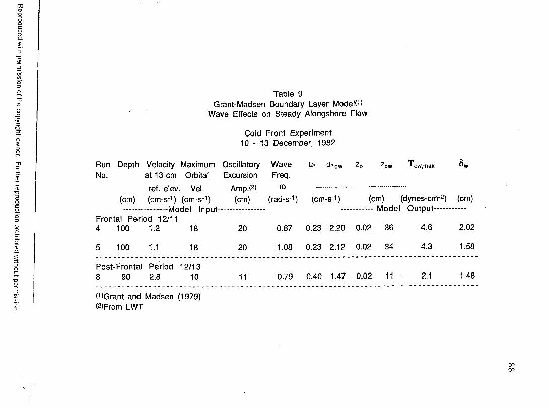
Reproduced
with perm
ission of the
copyright ow
ner. Further
reproduction prohibited
without
permission
Table 9Grant-Madsen Boundary Layer ModelO)
Wave Effects on Steady Alongshore Flow
Cold Front Experiment 1 0 - 1 3 December, 1982
-cwRun Depth Velocity Maximum Oscillatory Wave u* u*cw ;No. at 13 cm Orbital Excursion Freq.
ref. elev. Vel. Amp.(2) 05 ----------------(cm) (cm-s-1) (cm-s-1) (cm) (rad-s-1) (cm-s-1).......................Model Input........................ ........
Frontal Period 12/114 100 1.2 18 20 0.87 0.23 2.20 0.02 36
cw.max 'w
(cm) (dynes-cnr2) (cm) — Model Output................
100 1.1 18 20 1.08 0.23 2.12 0.02 34
4.6
4.3
2.02
1.58
Post-Frontal Period 12/13 8 90 2.8 10 11 0.79 0.40 1.47 0.02 11 2.1 1.48
OIGrant and Madsen (1979) (2)From LWT
OOoo

89
on the steady current as the combination of physical roughness, and the non
linear interaction of oscillatory and non-oscillatory flows in the WBL. This
resistance is transmitted to the flow interior in calculated values for u* (Table
9) which are nearly an order of magnitude lower than estimates derived from
the three-point velocity measurements given in Table 8. As a result, the
Grant-Madsen model predicts, for all the alongshore runs, velocity profiles
far steeper than the characteristic profiles shown in Figure 27. This
observation suggests that the current does not "feel" the drag generated in the
WBL, at least to the degree predicted by the model. One explanation for this
result may be that W BL turbulence, while important for maintaining
sediment in suspension close to the bed, is largely destroyed before it reaches
the interior of the flow.
An assumption of neutral stability, or the lack of significant turbulence
damping features in the flow, is implicit in both boundary layer models introduced thusfar. The increased slope (decreased u*) and lower z0 which
characterize the post-frontal velocity profile (run 8) in Figure 27, relative to
those from the two earlier runs is strongly suggestive of a change from a
stably stratified flow to one that is more neutral. Gradients in suspended
sediment concentration, like those due to salinity and temperature, can
produce a stable density field capable of inhibiting the vertical eddy diffusive
flux of turbulence (Smith and McLean 1977a). The suspended sediment
profiles shown in Figure 22, and the more complete data in Table 4, clearly
indicate the presence of a significant near-bottom concentration gradient
during runs 4 and 5, which was developed to a far lesser degree during run 8.
Gravity acts on the suspended sediment particles to oppose the upward
flux of turbulence produced by shear at the bed. The flux Richardson
Reproduced with permission of the copyright owner. Further reproduction prohibited without permission.

90
number provides a dimensionless measure of the relative magnitudes of these
forces. Smith and McLean (1977a) give the appropriate form of this ratio as:
(ps-p) dCs duR f = - g r~ ~ ■ —1(~)-2 (8)
p dz dz
where g is the force of gravity, dCs/dz is the volumetric sediment
concentration gradient (z positive up), du/dz is the horizontal velocity
gradient, and ps and p are the respective densities of the sediment and the
fluid. It can be seen that the gravity force, which acts on the excess mass of
sediment, represented by the bracketed term, is balanced against turbulence
produced by the velocity gradient. A flow characterized by a positive Rf
number is stably stratified, and acts as a sink for turbulent energy. Rf values
calculated for the velocity and suspended sediment gradients between 13 and
30 cm elevations during the alongshore runs range from +0.01 for run 8 to
+0.10 in run 5. At values of Rf greater than approximately +0.20,
laboratory experiments show that turbulent flux is completely suppressed
(Tennekes and Lumley 1972, p. 99).
Einstein and Krone (1962) found that differential consolidation of
fluid mud, a process which reduces water content in the lower part of a layer
at a more rapid rate than in the upper part, results in a characteristic increase
in sediment concentration with decreasing elevation above the bed. If fluid
mud was present below the 10 cm elevation o f the bottom-most sampler
during runs 4 and 5, and turbulence associated with the wave motion is generated within a W BL 1 to 2 cm thick, the magnitude of the R f number
might be expected to increase at least to the top of the WBL. The effect of
Reproduced with permission of the copyright owner. Further reproduction prohibited without permission./

91
such a stable density gradient will be to limit the vertical flux of turbulence
generated at the bed and thereby restrict sediment dispersal into the flow
interior.
One consequence of a restriction on the vertical flux of turbulence is
the emergence of a mechanism whereby a coherent fluid mud layer might be
transported in the direction of the mean flow. As Einstein and Krone (1962)
argued cogently 24 years ago, the vertical density and yield strength
gradients which characterize such suspensions render their transport en
masse by a uni-directional current alone improbable. Shear stress applied
only at the upper surface would initiate movement there first, with the result
that sediment would be stripped off and dispersed, while the denser
suspension closer to the bed remained stationary. Returning once more to the
B-L-S model (Fig. 28), however, we note that a sorting mechanism which
acts to segregate silt particles from a much larger population of clay floes in
the mixed suspension above the high shear zone must cause a break in the
sediment concentration gradient close to the bed. Given the relationship
between sediment concentration and yield strength, a concentration drop
imposed by shear at the bottom of a fluid mud layer would also be a point of
reduced yield strength. Transport of an intact fluid mud layer might then
occur, under the influence of shear exerted at its upper margin, along a shear
plane defined in 2 dimensions by the drop in yield strength at the top of the
high shear zone, in this case the WBL.
KINEMATICS OF FLUID MUD DEPOSITION AT THE SHOREFACE
Having developed the potential for transport of sediments contained
within a fluid mud layer under the influence of a unidirectional flow, the task
is now to identify such flows nearshore, particularly those with an onshore
Reproduced with permission of the copyright owner. Further reproduction prohibited without permission./

92
orientation. A re-examination o f the characteristic alongshore velocity
profiles (Fig. 27) suggests, however, that near-bottom current velocities in
these steady flows are so low that significant transport of sediment in a fluid
mud layer would be unlikely. All nearshore flows monitored during the cold
front experiment were not steady, however, and would not be expected to
reflect this equilibrium condition. This is particularly true of the shore-
normal flows observed, which, though sometimes logarithmic, continually
undergo acceleration and deceleration. This evolution is apparent in the
sequence o f velocity profiles from the low-frequency flow event captured
during run 3 (Fig. 25). Unlike the characteristic alongshore profiles,
velocity profiles associated with shore-normal flow suggest a potential for
non-equilibrium sediment transport close to the bed.
As noted previously, the low-frequency fluctuations in water level,
which are correlated with significant unsteady onshore-offshore flow, have
characteristics of a standing wave with an antinode at the shoreline and an
offshore node. Suhayda (1972) has shown that, for a linear wave field on a
sloping bottom, the frequency of a standing wave which has a node X meters
offshore is given by:
2.4 (g tan <X>)l/2f ------------------------------------------------------------ ( 9 )
4 tcX1/2
where tan O is the bottom slope. The period of the low frequency oscillation
in run 3 (Fig. 24) is estimated to be 600 s (0.0017 cps). The bottom slope is
0.004. Equation (9) can be rearranged to solve for the distance of the node
from shore,
with permission of the copyright owner. Further reproduction prohibited without permission.

93
5.76 g tan OX = -------------- (10)
(4 7 i f ) 2
which, in this case, is found to be 400 m.
It was observed that the amplitude of the low frequency oscillations
increases in the direction of the shoreline or antinode. In the present
example, the amplitude (H/2) of the low-frequency oscillation at sensor B
was 4.7 cm. The amplitude at sensor A, 10 m seaward, was 0.17 cm less, a
value which yields a maximum between-sensor slope of the still water
surface, tan N, of 0.00017. When this slope is linearly extrapolated offshore,
the node position is predicted to lie 369 m from the shoreline, a value in
reasonable agreement with the result from Equation (10).
The shoreface geometry at station 6 is shown schematically in Figure
29. A control volume approach was adopted to estimate the depth and time-
averaged velocities required to accomodate standing wave-induced flux
through water column cross-sections spaced at 25 m intervals along the
shore-normal transit shown in this figure. Onshore/offshore velocities
between the shoreline and 800 m offshore were calculated for 3 standing
waves, each with a 4.7 cm amplitude at sensor B, but with node positions
ranging from 200 to 800 m offshore, and the corresponding periods
determined from Equation (9). Results are plotted in Figure 30a for
conditions of rising water at the shoreline antinode. Except for a change in
sign, the results are identical for falling water conditions.
Reproduced with permission of the copyright owner. Further reproduction prohibited without permission.

1.0
ANTINODEANTINODE TAN N NODE
0 .5
800I6 0 04 0 02 0 0
P ressu reS e n so rs
5.76g tancp- ° - 5 r ( b ) x^ V ( a ) X=( 4 n f )
/ /S . TAN0
- 1 . 5
- 2.0
- 2 . 5
Figure 29. Generalized shoreface geometry, showing slopes used in determining standing wave node position, and changes in the cross- section affecting cross-shore velocities.
Reproduced with permission of the copyright owner. Further reproduction prohibited without permission.
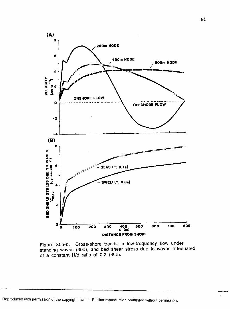
95
(A)
200m NODE
400m NODE800m NODE
i"'*"‘*......
>HOo- IUl>
ONSHORE FLOWOFFSHORE FLOW
- 2
-4
l i t * '
.1*'*“ — SEAS (T: 3.1s)
0 "
— SWELUT: 6.8s)
_i_____ .— .— i100 200 300 400
X (m)DISTANCE FROM SHORE
500 600 700 800
Figure 30a-b. Cross-shore trends in low-frequency flow under standing waves (30a), and bed shear stress due to waves attenuated at a constant H/d ratio of 0.2 (30b).
Reproduced with permission of the copyright owner. Further reproduction prohibited without permission.

96
The model predicts that a standing wave with the amplitude observed
during run 3, and a node located 400 m offshore, would generate a mean
depth-averaged onshore velocity during the rising water phase of 3.8 cm-s-1
at sensor B. This is twice the actual depth- and time-averaged low frequency
onshore velocity monitored at this point between 600 and 900 s in run 3 (Fig.
24), but, given the many simplifications, the result is encouraging.
It can be seen in Figure 30a that, although the higher frequency,
shorter wavelength standing waves generate greater shore-normal velocities
for the same amplitude, cross-shore current speeds associated with a 750 s
oscillation (node 800 m from shore) would still be significant. The shape of
these curves is more important than the velocities calculated in this example.
For all three standing waves, the onshore velocity peak is shifted significantly
shoreward of the node position it would occupy if the bottom did not slope.
As a result, deceleration of onshore, and acceleration of offshore flows, due
to standing waves of any period, will be most pronounced within 100 m of
the shoreface. The existence of waxing and waning flows at a position fixed
by geometry is of great interest with respect to nearshore sediment transport
and deposition. It does not completely explain preferential deposition at the
shoreface, however, as both onshore and offshore velocities under a standing
wave are of the same magnitude.
Waves observed during the frontal and post-frontal periods were
attenuated completely before reaching the shoreface. Wells (1978) found
that attenuation across a Surinam mud bank was a linear function of depth.
The characteristic ratio of H/d identified in Surinam (0.2) also appears to act
as a limit to wave heights monitored in this study (Fig. 20). If this ratio is
assumed to be constant across the nearshore profile shown in Figure 29, peak
Reproduced with permission of the copyright owner. Further reproduction prohibited without permission./

97
bed shear stresses generated by waves alone may be estimated at any point
using an equation derived by Krone (1976) from LWT:
pjc flHrms/T
T m ax = 1-7 p (— -------------------------------- (11)T \x sinh (2jcd/L)
where ji is the coefficient of viscosity. The empirical coefficient of 1.7 is
included to account for laboratory results which indicate that, without it, this
equation underestimates shear stress based on significant wave height (H j/3 =
1.4 Hrms) by 20 percent (Krone 1976). It should be noted that, for shallow
water waves, both the period, T, and the depth, d, enter Equation (11)
through the wavelenth, L = T (gd)l /2} as well as where explicitly stated.
Results of shear stress determinations at 25 m intervals are plotted in Figure
30b for the characteristic sea and swell wave periods, 3.1 and 6.8 s,
respectively.
Two points arise from this analysis. First, it is clear that shorter
wavelength seas generate greater peak bed shear stresses than do swells of
equal amplitude, attenuated at the same rate. Second, shear stresses due to
waves of both periods increase with distance from the shoreline.
The presence of a shore-normal wave shear stress gradient which is the
reverse of that found on surf-dominated coasts has clear implications for
sediment deposition, particularly when considered together with the
possibility for cross-shore transport of fluid mud. If a fluid mud layer
formed and maintained at one level of WBL shear is carried shoreward, the
potential exists for deposition when its yield strength exceeds the lower
Reproduced with permission of the copyright owner. Further reproduction prohibited without permission.
/

98
nearshore WBL shear. Mud transported offshore remains supported and is
less likely to deposit.The effect of wave period is less apparent. Though hardly conclusive
on this point, the results suggest that high-frequency seas may inhibit
development of a fluid mud layer. Wells (1978) has indicated that the
converse also appears to be true; that is, that fluid mud filters high-frequency
waves from the spectrum. Data from the chenier plain do not permit
resolution of this question. The thickness of the W BL is, however, known to
be a function of frequency (Eq. 7). It is probable that other factors related to
the state of development of the WBL may also influence the ability of a flow
to support a coherent fluid mud layer, particularly, if, as in most real
systems, several wave trains are superposed. The theoretical difficulties in
characterizing a simple system, with only two appropriate boundary layer
length scales, are significant, but they are magnified dramatically if multiple
WBL length scales must be considered. A range of frequencies then become
important, and, particularly for locally generated seas, a variety of
directions.Mud deposition through boundary layer dumping is triggered in the
modified B-L-S model whenever the yield strength of the fluid mud
suspension attains equivalence with wave generated shear stress. An abrupt
reduction in near-bottom suspended sediment concentration would occur
immediately after each dumping event. This reduction would permit
reformation of the WBL above the new deposit. The cycle of sediment
sorting, concentrating, and dumping might then be repeated, and give rise to
the stacked sequences noted in mudflat cores. It is important to note that
accretion can occur, however, only if sediment continues to be added
Reproduced with permission of the copyright owner. Further reproduction prohibited without permission.
/

99
primarily from above the WBL, rather than from resuspension of sediment
already deposited.
High rates of mudflat sedimentation through WBL dumping are
possible if suspended sediment is continuously advected into the vicinity of
the shoreface. No high-resolution measurements of the rate of mudflat
sedimentation have been made. The best available observation is that of
Morgan et al. (1958) who noted that a layer of mud 18 inches thick (46 cm)
was deposited over a span of 3 days. Based on this, a lower bound may be
placed on the sedimentation rate if it is assumed.that the deposit has a density
of 1.3 g-cm-3, and, less realistically, that sedimentation was continuous
throughout the 3 day period. A deposition rate is calculated on the order of 1
g-m -2-s-l, 2000 times greater than the average rate for continental shelf
sedimentation estimated by McCave (1984).
Instantaneous rates several orders of magnitude higher could apply
during the boundary layer dumping events envisioned, such that a single bed
10 cm thick might be deposited in a matter of seconds. Sedimentation rates
ranging between 2 and 50 kg-m-2-s-l are calculated if deposition is assumed
to occur over a period of 1 to 30 s, and the density of the deposit formed is
again estimated at 1.3 g-cm-3. Deposition at this rate from a i m thick water
column implies a depth-averaged sediment concentration of nearly 50 g -H .
If the nearshore introduction of sediments at these concentrations is required
for mudflat sedimentation, it is clear why mudflat formation is such an
intermittent process, and, more specifically, why deposition did not occur
during the cold front monitored. The highest depth-averaged concentrations
found during this experiment, estimated by logarithmically extrapolating the
mean concentration data from the frontal period to the bed, were less than
Reproduced with permission of the copyright owner. Further reproduction prohibited without permission.
/
100
2.5 g -l" l. One interpretation of this scaling is that, during the periods when
mudflat sedimentation is active, the flux of mud advected to the coast must be
an order of magnitude higher than was observed during the cold front
experiment.
The stated purpose of this investigation is to examine the processes by
which a coast incorporates influxes of mud intercepted from a shelf dispersal
system. A purely kinematic model has been proposed to explain preferential
deposition of mud at the shoreface. This is an important first step. Results of
the long-term shoreline monitoring program, historical data, and the
sedimentation rate scaling just concluded, indicate, however, that factors
affecting sediment supply operate at far greater temporal and spatial scales
than have been considered thusfar. Attention is directed now to these
regional influences.
SHELF SEDIMENT DISPERSAL
The high abundances of illite and illite-smectite mixed-layer clays in
mudflat sediment suggest an origin in modem Atchafalaya flood discharge,
rather than reworked older shelf deposits (Johns and Grim 1958, Brooks
1970), or low-flow Atchafalaya input (Van Heerden 1983), both of which
tend to be richer in smectite. A close temporal connection between mudflat
sedimentation on the chenier plain and the flux of Atchafalaya sediments to
the shelf seems likely. Littoral mud deposition in the study area occurred
only during late winter and in the spring when the River was in flood. The
high winds, waves, and water level fluctuations accompanying front passages
are also important, but frontal weather systems traverse this region from
September through April, a far longer period, which includes, but is not
Reproduced with permission of the copyright owner. Further reproduction prohibited without permission/

101
limited to, the 5 month window identified for coastal deposition. The fact
that mud sedimentation did not occur during the December experiment, and
does not occur generally, prior to peak flow on the Atchafalaya in late winter
and early spring, suggests the need for a volume or availability of advected
sediments nearshore which is attained only at that time.
The dynamical environment on the shelf is quite different from that
identified nearshore along the muddy coast. Turbulent shelf currents have
the potential to transport high concentrations of fine-grained sediments
dispersed through the full depth of the flow, rather than confined close to the
bed. Sediment concentrations at the surface within the shelf "mud stream"
offshore of Atchafalaya Bay range up to 800 m g -H during river flood
(Wells and Kemp 1981), and are higher than any measured near-surface on
the muddy coast (Table 4). This sediment appears to become concentrated in
near-bottom fluid mud layers where the characteristic turbulent eddy length
scale within the shelf flow is restricted, perhaps by a decrease in depth, and
WBL shear stress prevents deposition. Unsteady onshore-offshore flows,
associated with the wind-forced, shore-amplified water level oscillations
which precede front passage, then capture fluid mud for transport across the
shear stress gradient developed under progressively attenuated waves.
Stacked graded and laminated mud beds form accretionary deposits at the
shoreface through repeated dumping of fluid mud suspensions by the wave
boundary layer. Coastal progradation occurs when these mudflat deposits
are stabilized by marsh vegetation.
While the kinematics remain the same, a direct temporal link with the
period of river flood is not required in the special case of mudflat deposition
during hurricanes. Under normal cold front conditions, deep-water waves
Reproduced with permission of the copyright owner. Further reproduction prohibited without permission.

102
offshore are too small to exert significant shear stress at the bed (Adams et al.
1982). Hurricane-generated waves, however, would be capable of
reworking and suspending large volumes of mud from deep-water shelf
storage sites. Fluid mud might form farther offshore, and be transported a
greater distance cross-shelf, by the "standing wave" flow associated with a
storm surge several meters in magnitude.
FUTURE CHENIER PLAIN PROGRADATION
The spread of clastic beaches in the area east of Freshwater Bayou
Canal provides an indication that littoral mud deposition is modulated by
changes in sediment flux over periods far longer than a single year. Mudflat
deposition and shoreline progradation west of the Canal continues at
approximately the same rate today as during the 1950’s and 1960's (Morgan
and Larimore 1957, Coleman 1966, Morgan and Morgan 1983). The lateral
extent of the muddy coast has decreased, however, as the eastern margin of
the zone of active mudflat formation has shifted 10 km west without any
corresponding extension on its western boundary. It is clear that less mud is
being deposited in the study area today than 20 or 30 years ago.
The subaerial delta in Atchafalaya Bay is now 13 years old, and covers
nearly 30 km^ (Wells et al. 1983). Sediments entering the bay in river flow
are dispersed across the delta through an intricate system of bifurcating
channels which did not exist 20 years ago. Prior to the emergence of sandy
islands, scour by waves maintained a constant depth and limited
sedimentation in the shallow, open bay (Thompson 1955). Now, fine
grained sediments which formerly reached the shelf, particularly during low
flow periods, are deposited in channel fills and on extensive algal flats
Reproduced with permission of the copyright owner. Further reproduction prohibited without permission./

103
formed between natural levee ridges (Van Heerden et al. 1981, Van Heerden
1983). The amount of mud trapped relative to total fine-grained sediment
flux to the shelf is unknown, but evidence from the chenier plain suggests that
the presence of the new delta may be exerting an influence on downdrift
deposition.
Wells et al. (1983) have projected that the subaerial delta will continue
to grow within the confines of Atchafalaya Bay through the end of this
century, but will emerge on the inner shelf by 2030. Mudflat deposition on
the eastern chenier plain may, therefore, be expected to continue at
approximately the rate observed in this study for the next 50 years. When
delta development begins on the open coast outside the shell reef, it will be
exposed to greater erosion by waves, and can be expected to expand at a
slower rate. More fine-grained sediments will be delivered to the coastal
mud stream, particularly under low flow conditions, and mudflat
sedimentation downdrift should increase dramatically.
IMPLICATIONS FOR OTHER COASTS AND THE GEOLOGIC RECORD
Observations made during this study indicate that the only strict
requirement for mud sedimentation at the shoreface is that a large flux of
fine-grained sediments must be delivered close to shore. A high wave energy
regime, for example, is no barrier, as waves, and die boundary layers they
generate, play an important role in the formation of fluid mud layers
nearshore. A large tidal excursion, likewise, poses no restriction on fine
grained sedimentation at the coast. Rapid changes in water level are critical
to the onshore transport of sediment contained in fluid mud layers, therefore
semi-diurnal, rather than diurnal tides should be more effective for the same
range. A 3.2 m semi-diurnal tide almost certainly provides the same forcing
Reproduced with permission of the copyright owner. Further reproduction prohibited without permission.

104
for cross-shore flow along the Surinam coast (Wells and Coleman 1981b,
Rine and Ginsburg 1985) as the wind-generated water level oscillations
observed on Louisiana's chenier plain. Where a turbid coastal current is not
developed, large storms can cause intermittent mud deposition at the beach.
Storm waves suspend large volumes of fine-grained sediments stored
offshore, and storm surges provide the cross-shore flows necessary for
transport to the shoreface. Such deposition has been observed outside of the
period of river flood along the Louisiana coast (Morgan et al. 1958) and on
the Rio Grande do Sul coast of southern Brazil (Delaney 1963, Martins et al.
1979).
Large-scale coastal progradation associated with mud deposition at the
shoreface requires a continuous, rather than intermittent, supply o f large
volumes of mud, as sediment-starved littoral deposits are quickly destroyed
by normal wave action. Continuity of fine-grained sediment provenance is
dependent on the steadiness of sediment introduction to the shelf, and on the
spatial stability of shelf dispersal. Seasonal and longer-term changes in these
factors characterize all real systems to a greater or lesser degree. Thus, all
muddy coasts can be expected to exhibit a mix,proportionate to this
variability, of coarse-grained and muddy facies at the receiving shoreface.
Onshore transport of fluid mud by unsteady flow under standing
waves is developed only on the foreshore, where the significant change in
bottom slope plays an important role. This restricts mud deposition to
shallow water in the immediate vicinity of the shoreface, and thereby limits
the maximum thickness of the deposit.
Intermittent littoral mud deposits associated with storms will have
poor preservation potential, but mudflats that form part of a major
B-«rr*iWW
Reproduced with permission of the copyright owner. Further reproduction prohibited without permission/

105
progradational sequence may survive if regional subsidence or uplift
produce gradual changes in the relative position of sea level. In cross-
section, all shoreface mud deposits should exhibit the characteristic laminated
and graded bedding which Stow and Bowen (1980) ascribe to boundary layer
sorting. Lower beds will be little disturbed by marine organisms, because of
the high rate of deposition associated with boundary layer dumping. Layers
close to the upper, subaerially exposed surface will, however, display cracks,
burrows, trails, and evidence of rooting.
W alker and Harms (1971,1976) have described in detail what they
interpret as coastal mudflat deposits from an ancient chenier plain setting.
This facies is found in more than 20 predominantly muddy, marine-
nonmarine sequences in the Upper Devonian Catskill Formation of central
Pennsylvania. The sequences represent episodes of coastal progradation on a
subsiding coast, which, in some cases, can be traced for 30 km down basin.
Transgressive sands define the boundaries of each cycle.
Indeed, the shales which lie at the top of the regressive sequences
display precisely the structures which are predicted for an accreting littoral
mudflat deposit. Rootlets and dessication cracks in some cases occur less than
2 m above marine faunas.
Reproduced with permission of the copyright owner. Further reproduction prohibited without permission.
/

CONCLUSIONS
Fieldwork conducted between December, 1981, and May, 1983, along
a 30 km section of Louisiana's chenier plain coast disclosed widespread
shoreline retreat, averaging 5 to 10 m-yr-1. Intermittent sedimentation of
shore-welded mudflats was observed, however, to cause localized reversal of
this erosional trend on a 15 km long muddy coast extending west from
Freshwater Bayou Canal. This deposition takes place only in late winter and
early spring, synchronous with peak flood on the Atchafalaya River, which
discharges into Atchafalaya Bay 100 km to the east o f the study area.
A four day investigation of nearshore dynamics, conducted over the
broad range of wave and current conditions which accompanied passage of a
winter cold front showed that waves incident on the muddy shoreface were
well described by shallow water linear wave theory, but exhibited the
progressive nearshore attenuation and absence of breaking described by
Coleman and Wells (1981a) from Surinam. This attenuation gives rise to an
onshore decrease in wave shear stress at the bed which is the reverse of that
noted on clastic coasts dominated by surf zone processes.
A significant vertical gradient in suspended sediment concentration
was observed under low-frequency swell which was not developed when
higher-frequency seas formed an important component of the wave energy
spectrum. Concentrations 10 cm above the bed ranged up to the lower limit
for fluid mud (Einstein and Krone 1962) when this gradient was present.
The existence of a concentrated mud suspension near bottom at this time was
also apparent in elevated estimates of bed roughness identified in logarithmic
velocity profiles of the steady alongshore flow.
106
Reproduced with permission of the copyright owner. Further reproduction prohibited without permission.

107
The formation of fluid mud layers appears to occur when sediments
suspended through the full depth of the coastal boundary current are
introduced into a less turbulent environment nearshore, but are prevented
from depositing by high shear stresses close to the bed within a wave
boundary layer (WBL). An important property of fine-grained sediment
suspensions at fluid mud concentrations, which was demonstrated for the
mudflat sediments in this study, is the development o f yield strength, which is
the ability to resist deformation up to some critical level of shear stress
(Einstein 1941). Concentration of the sediment load near-bottom in a gel
like fluid mud layer decouples the steady alongshore flow from turbulence
generated within the 1 to 2 cm thick WBL. Adjustment of the steady current
velocity profile to the presence of a fluid mud layer restricts further
transport of this sediment alongshore. Cross-shore transport of sediment
contained in this layer is proposed, however, under the influence of unsteady
onshore-offshore flows which were observed to be associated with low-
frequency, shore-amplified water level oscillations. These oscillations,
apparently forced by pre-frontal winds, have characteristics of a standing
wave with a shoreline antinode. Because of the slope of the foreshore,
onshore and offshore flows associated with standing wave-like motion
experience maximum acceleration and deceleration within 100 m of the
shore.
Intact transport of the fluid mud layer in the direction of an
accelerating flow is proposed as a consequence of the wave-induced
oscillatory shear stress exerted at its lower margin. Boundary-layer sorting
of cohesive and non-cohesive sediments at this point, of the type described by
Stow and Bowen (1980), implies the existence of a break in the vertical
Reproduced with permission of the copyright owner. Further reproduction prohibited without permission.
/
108
sediment concentration gradient at the top of the WBL. Because of the
relationship between sediment concentration and yield strength in fine
grained sediment suspensions in the fluid mud range, yield strength should
also exhibit a significant reduction at this point. Expanded to two
dimensions, this point of weakness forms a plane along which the fluid mud
layer can move in response to shear exerted by an accelerating flow at its
upper margin.
Rapid deposition of the fluid mud layer is proposed through a
boundary layer dumping process when the yield strength of the fluid mud
layer supported above the WBL reaches equivalence with WBL shear stress.
The onshore decreasing shear stress gradient developed under attenuating
waves gives rise to preferential deposition close to shore. Repeated
sequences of boundary layer sorting, followed by "freezing" of the fluid mud
layer, give rise to the vertically stacked 2 to 10 cm thick silt/shell + mud beds
which characterize mudflat cores. Sedimentation rates associated with this
process are estimated to be as high as 50 kg-m-2-s-l.
Shoreface accretion by boundary layer dumping gives rise to a
characteristic internal mudflat structure which exhibits little disturbance by
burrowing marine organisms. Littoral mudflats deposited as part of a major
coastal progradational episode have good preservation potential on a
subsiding coast, and are well displayed in the regressive sequences described
by Walker and Harms (1971,1976) from the Middle Devonian.
The spread of clastic beaches into an area of former mudflat deposition
in the eastern half of the chenier plain study area indicates that the flux of
mud to this coast has decreased over the past 20 years. Trapping of fine
grained sediment in the subaerial delta which has formed in Atchafalaya Bay
Reproduced with permission of the copyright owner. Further reproduction prohibited without permission.

109
since 1973 is proposed as one possible cause for this reduction. Because of
the close temporal relationship between mudflat formation and fine-grained
sediment flux from Atchafalaya Bay to the shelf, no increase in littoral mud
sedimentation on the chenier plain can be expected until 2030, when the
subaerial delta is projected to expand onto the inner shelf (Wells et al. 1983).
Regional coastal retreat along the chenier plain is, therefore, likely to
continue for the next 50 years. Renewed large-scale advance of the marsh
shoreline across mudflats into the Gulf of Mexico, the progradational process
which has characterized this coast generally over the past 3000 years, is
predicted when the new delta emerges from Atchafalaya Bay, and is exposed
to increased wave action on the shelf.
Some variation of the dynamics proposed for fluid mud formation and
transport in the littoral setting investigated are likely to be manifested in the
many shelf and estuarine environments where highly concentrated near
bottom suspensions of fine-grained sediment are observed. Evidence
acquired nearshore, in this study, of the boundary layer sorting originally
proposed by Stow and Bowen (1980) to explain shelf margin turbidite
sedimentation suggests that this mechanism may be important wherever
multiple boundary layer length scales are involved.
The dynamical inferences drawn by Stow and Bowen (1980) from
sedimentological evidence, coupled with analysis of time-series
measurements made on muddy coasts, begun by Wells and Coleman (1981a,
b), and continued in this study, have led to proposal o f a new mode for fine
grained sediment transport in the marine environment. At the heart of this
progress is a recognition that properties of fine-grained sediment
suspensions, yield strength, for example, which do not emerge from
Reproduced with permission of the copyright owner. Further reproduction prohibited without permission.
/

110
consideration of the behavior of individual particles, play an important role
in mud sedimentation.
The importance of continued field research is clear, as some processes,
like wave attenuation, which are critical to fluid mud formation, transport,
and deposition, are poorly developed at laboratory scales. The results of this
work suggest that the world's many muddy shorelines, which remain largely
untouched by the most basic research efforts, are appropriate "laboratories"
for the investigation of a broad spectrum of fine-grained sediment problems
which also arise in other environments less accessible for study.
Reproduced with permission of the copyright owner. Further reproduction prohibited without permission.

B IB L IO G R A P H Y
Adams, C.E., and Weatherly, G.L., 1981a, Suspended-sediment
transport and benthic boundary-layer dynamics:
Marine Geology, v. 42, p. 1-18.
__________________________ , 1981b, Some effects of suspended-
sediment stratification on an oceanic bottom boundary layer:
Jour. Geophys. Res., v. 86, p. 4161-4172.
Adams, C.E., Wells, J.T., and Coleman, J.M., 1982, Sediment transport
on the central Louisiana continental shelf: implications for
the developing Atchafalaya River delta: Contrib. Mar. Sci., v. 25,
p. 133-148.
Alishahi, M.R., and Krone, R.B., 1964, Suspension of cohesive
sediments by wind-generated waves: Hydraulic Engr.
Laboratory, Univ. Cal., Berkeley, Tech. Rept. HEL-2-9, 24 p.
Allersma, E., 1971, Mud on the oceanic shelf off Guiana, in
Symposium on Investigations and Resources of the Carribbean
Sea and Adjacent Regions: UNESCO, Paris, p. 193-203.
Angelovic, J.W., 1976, Physical oceanography, in NOAA Final Report,
Environmental Studies of the South Texas Continental Shelf:
U.S. Dept, of Commerce, Gulf Fisheries Center, Galveston, TX.
111
Reproduced with permission of the copyright owner. Further reproduction prohibited without permission.

Bailey, A.M., 1934, Chenier au Tigre: La. Cons. Rev., v. 4(2), p. 9-11.
Beall, A.O., 1968, Sedimentary processes operative along the
western Louisiana shoreline: Jour. Sed. Petrology, v. 38, p.
869-877.
Bendat, J.S., and Piersol, G.G., 1980, Measurement and Analysis of
Random Data: New York, John Wiley and Sons, 302 p.
Bingham, E.C., 1922, Fluidity and Plasticity: New York, McGraw-Hill,
440 p.
Boussinesq, J., 1872, Theorie des ondes et de remous qui se
propagent le long d'un canal rectangulaire horizontal, en
communiquant au liquide contenu dans ce canal des vitesses
sensiblement paralleles de la surface au fond: J. Math. Pures
et Appliquees, v. 17, p. 55-108.
Brooks, R.A., 1970, Geochemical and mineralogical relationships in
the sediments on the Louisiana continental shelf [unpubl. Ph.D.
dissert.]: Louisiana State Univ., Baton Rouge, 97 p.
Byrne, J.V., LeRoy, D.O., and Riley, C.M., 1959, The Chenier Plain and
its stratigraphy, southwestern Louisiana: Trans. Gulf Coast
Assn. Geol. Soc., v. 9, p. 237-260.
Reproduced with permission of the copyright owner. Further reproduction prohibited without permission.

113
Carter, T.G., Liu, P.L-F., and Mei, C.C., 1973, Mass transport by waves
and offshore sand bedforms: ASCE, Jour. Waterways Harbors
Coastal Engr. Div., v. 99(WW2), p. 165-184.
Chuang, W.S., and Wiseman, W.J., Jr., 1983, Coastal sea-level
response to frontal passage on the Louisiana-Texas shelf: Jour.
Geophys. Res., v. 88, p. 2615-2620.
Cochrane, J.D., and Kelly, F.J., 1986, Low-frequency circulation on
the Texas-Louisiana continental shelf: Jour. Geophys. Res., v.
91, p. 10645-10659.
Coleman, J.M., 1966, Recent coastal sedimentation: central Louisiana coast:
Coastal Studies Series No. 17, Louisiana State Univ.,
Baton Rouge, 73 p.
Cooley, J.W., Lewis, P.A.W., and Welch, P.D., 1969, The fast Fourier
Transform and its applications: IEEE Trans, on Education, v. 12,
p. 27-34.
Cornish, V., 1898, On sea beaches and sand banks: Geog. Jour., v. 11,
p. 528-559.
Cratsley, D.W., 1975, Recent deltaic sedimentation, Atchafalaya Bay,
Louisiana [unpubl. M.S. thesis]: Louisiana State Univ., Baton Rouge,
142 p.
Reproduced with permission of the copyright owner. Further reproduction prohibited without permission.

114
Crout, R.L., 1983, Wind-driven, near-bottom currents over the west
Louisiana inner continental shelf [unpubl. Ph.D. dissert.]:
Louisiana State Univ., Baton Rouge, 117 p.
_________, Wiseman, W.J., Jr., and Chuang, W.S., 1984, Variability of
wind-driven currents, west Louisiana Inner Continental Shelf:
Contrib. Mar. Sci., v. 27, p. 1-11.
Csanady, G.T., 1977, The coastal jet conceptual model in the dynamics of
shallow seas in Goldberg, E.D., McCave, I.N., O'Brien, J.J., and J.H.
Steele, eds., The Sea: New York, Wiley-Interscience, v. 6, p. 117-144.
Daddio, E., Wiseman, W.J., Jr., and Murray, S.P., 1978, Inertial
currents over the inner shelf near 30° North: Jour. Phys.
Oceanogr., v. 8, p. 728-733.
Das, M.M., 1970, Study of Bingham shear strength of a deep marine
sediment by capillary viscometer in Einstein, H.A., and Wiegel,
R.L., eds., A Literature Review on Erosion and Deposition of
Sediment Near Structures in the Ocean: Hydraul. Engr. Lab.,
Univ. Calif., Berkeley, Final Rept. HEL 21-6, p. 2-1 - 2-13.
Dawson, T.H., 1978, Wave propagation over a deformable sea floor:
Ocean Engr., v. 5, p. 227-234.
Reproduced with permission of the copyright owner. Further reproduction prohibited without permission.

Delaney, P.J.V., 1966, Geology and geomorphology of the coastal plain
of Rio Grande do Sul, Brazil and Northern Uruguay: Coastal
Studies Series No. 15, Louisiana State Univ., Baton Rouge, 58 p.
Delft Hydraulics Laboratory, 1962, Demerara coastal investigation:
Delft, The Netherlands, 240 p.
Dinnel, S.P., and Wiseman,W.J., Jr., 1986, Fresh water on the west
Louisiana and Texas shelves: Cont. Shelf Res., v. 6, p. 765-784.
Dolan, R, Hayden, B., Homberger, G., Zieman, J., and Vincent, M., 1972,
Classification of the Coastal Environments of the World, Part
I, the Americas: Dept. Environmental Sciences, Univ. Virginia,
Tech. Rept 1,163 p.
Doyle, E.H., 1973, Soil-wave tank studies of marine soil instability:
Fifth Offshore Tech. Conf., Houston, Preprint 1901, p. II-753 -
11-766.
Drake, D.E., 1976, Suspended sediment transport and mud deposition
on continental shelves, in Stanley, D.J., and Swift, D.J.P., eds.,
Marine Sediment Transport and Environmental Management,
New York, Wiley Interscience, p. 127-158.
Reproduced with permission of the copyright owner. Further reproduction prohibited without permission.

1 1 6
Einstein, H.A., 1941, The viscosity of highly concentrated underflows and its
influence on mixing: Trans. Am. Geophys. Union, Hydrology
Section, p. 597-603.
___________ , and R.B. Krone, 1962, Experiments to determine modes
of cohesive sediment transport in salt water: Jour. Geophys.
Res. v. 67, p.1451-1461.
Eisma, D., and van der Marel,H.W., 1971, Marine muds along the
Guyana coast and their origin from the Amazon basin: Contrib.
Mineral. Petrology, v. 31, p. 321-334.
Faas, R.W., 1981, Rheological characteristics of Rappahannock
estuary muds, southeastern Virginia, U.S.A., in Holocene
Marine Sedimentation in the North Sea Basin, Int. Assn.
Sediment. Spec. Publ., v. 5, p. 505-515.
Femandez-Partagas, J., and Mooers, C.N.K., 1975, A subsynoptic study
of winter cold fronts in Florida: Monthly Weather Rev., v. 101,
p. 742-744.
Fisk, H.N., 1948, Geology of lower Mermentau River basin and control
structure sites: Definite Project Report, Mermentau River,
Louisiana, App. 2, U.S. Army Corps of Engineers, Miss. River
Comm., Vicksburg, MS., 41 p.
Reproduced with permission of the copyright owner. Further reproduction prohibited without permission.
/

Folk, R.L., 1954, The distinction between grain size and mineral
composition in sedimentary rock nomenclature: Jour. Geol., v.
62, p. 345-351.
, 1980, Petrology of Sedimentary Rocks, Austin, TX.,
Hemphill, 183 p.
Gade, H.G., 1958, Effects of a nonrigid, impermeable bottom on plane
surface waves in shallow water: Jour. Mar. Res., v. 16, p. 61-
82.
, 1959, Notes on the effect of elasticity of bottom
sediments to the energy dissipation of surface waves in
shallow water: Arch. Math. Natur., Oslo, v. 55, p. 69-80.
Gibbs, R.J., 1970, Circulation in the Amazon River estuary and
adjacent Atlantic Ocean: Jour. Marine Res., v. 28, p .l 13-123.
_________, 1976, Amazon River sediment transport in the Atlantic
Ocean: Geology, v. 4, p. 45-48.
Gould, H.R., and McFarlan, E, Jr., 1959, Geological history of the
Chenier Plain, southwestern Louisiana: Trans. G ulf Coast Assn.
Geol. Soc., v. 9, p. 261-270.
Reproduced with permission of the copyright owner. Further reproduction prohibited without permission.

Grant, W.D., and Madsen, O.S., 1979, Combined wave and current
interaction with a rough bottom: Jour. Geophys. Res. v. 84, p.
1797-1808.
Griffin, G.M., 1971, Interpretation of X-ray diffraction data, in
Carver, R.E., ed., Procedures in Sedimentary Petrology, New
York,Wiley Interscience, p. 541-569.
Ho, C., and Coleman, J.M., 1969, Consolidation and cementation of
Recent sediments in the Atchafalaya basin: Bull. Geol. Soc. Am.,
v. 80, p 183-192.
Hsiao, S.V., and Shemdin, O.H., 1980, Interaction of ocean waves with
a soft bottom: Jour. Phys. Oceanog., v. 10, p. 605-610.
Huntley, D.A., and Bowen, A.J., 1975, Field measurements of
nearshore velocities: Proc. 14th Conf. Coastal Engr.,
Copenhagen, p. 538-549.
Hydraulics Research Station, 1979, Port of Brisbane Siltation Study, Fifth
Report: Properties of Brisbane Mud: Hydraul. Res. Station,
Wallingford, Rep. E X 860 ,18 p.
Jenkins, G.M., and Watts, D.G., 1968, Spectral Analysis and its
Applications: San Francisco, Holden-Day, 525 p.
Reproduced with permission of the copyright owner. Further reproduction prohibited without permission.

Johns, W.D., and Grim, R.E., 1958, Clay mineral composition of Recent
sediments from the Mississippi River delta: Jour. Sed.
Petrology, v. 28, p. 186-199.
Johnson, A.M., 1970, Physical Properties in Geology: San Francisco,
Freeman, Cooper & Co., 577 p.
Kaczorowski, R.T., and Gemant, R.E., 1980, Stratigraphy and coastal
processes of the Louisiana Chenier Plain and Louisiana Chenier Plain
microfossil associations, in The Sedimentary Environments of the
Louisiana Coastal Plain: Field Trip Guidebook for the 30th Annual
Convention of the Gulf Coast Assn. of Geol. Soc., Lafayette, LA., p. 1-
72.
Kana, T.W., 1979, Surf zone measurements of suspended sediment:
Proc. 16th Conf. Coastal Engr., Hamburg, p. 1725-1743.
Keulegan, G.H., and Krumbein, W.C., 1949, Stable configuration of
bottom slope in a shallow sea and its bearing on geological
processes: Trans. Am. Geophys. Union, v. 30, p. 855-861.
Kolb, C.R., and Van Lopik, J.R., 1958, Geology of Mississippi River
deltaic plain, southeastern Louisiana: U.S. Army Corps of
Engineers, Waterways Exper. Sta., Vicksburg, MS., Reports 3-
483, 3-484.
Reproduced with permission of the copyright owner. Further reproduction prohibited without permission.

Komar, P.D., 1976, Beach Processes and Sedimentation: Englewood
Cliffs, New Jersey, Prentice-Hall, 429 p.
Krone, R.B., 1962, Flume studies of the transport of sediment in
estuarial shoaling processes: Hydraulic Engr. and Sanitaiy Engr.
Res. Laboratory, Univ. Calif., Berkeley, 110 p.
_________, 1963, A study of rheologic properties of estuarial
sediments: Sanitaiy Engr. Res. Laboratory Report 63-8, Univ.
Cal., Berkeley, 91 p.
• 1976, Engineering interest in the benthic boundary layer, in
McCave, I.N., ed., The Benthic Boundary Layer, New York,
Plenum Publ., p. 143-156.
Lanesky, D.E., Logan, B.W., Brown, R.G., and Hine, A.C., 1979, A new
approach to portable vibracoring underwater and on land: Jour.
Sed. Petrology, v. 49, p. 654-657.
Lhermitte, P., 1960, Mouvements des materiaux de fond sous faction de la
houle: Proc. 7th Conf. Coastal Engr., The Hague, p. 211 - 261.
Longuet-Higgins, M.S., 1953, Mass transport in water waves: Phil.
Trans. Roy. Soc. London, v. 245, p. 535-581.
Reproduced with permission of the copyright owner. Further reproduction prohibited without permission.

121
Maa, P.-Y, 1986, Erosion of soft muds by waves [unpubl. Ph.D. dissert.]:
Univ. Fla., Gainesville, 275 p.
________ , and Mehta, A. J., in press, Considerations on bed response in wave
resuspension of muds, in Kuo, A.Y., ed., Estuarine Circulation,
Clinton, New Jersey, Humana Press.
Macpherson, H., 1980, The attenuation of water waves over a non-
rigid bed: Jour. Fluid Mechanics, v. 97, p. 721-742.
Mallard, W.W., and Dalrymple,R.A., 1977, Water waves propagating
over a deformable bottom: Proc. 9th Offshore Tech. Conf.,
Houston, TX., v. 3, p. 141-146.
Manner, H.A., 1954, Tides and sea level in the Gulf of Mexico in U.S.
Fish. Wildl. Serv., ed., Gulf of Mexico, its Origin, Waters and
Marine Life, Fish. Bull. v. 89, p. 101-118.
Martins, L.R., Martins, I.R., Villwock, J.A., and Calliari, L.J., 1979,
Occorrencia de lama na praia do cassino (RS): Separata Dos
Anais 1978,22 p.
McCave, I.N., 1972, Transport and escape of fine-grained sediments
from shelf areas, in Swift, D.J.P., Duane, D.B., and Pilkey, O.H.,
eds., Shelf Sediment Transport: Process and Pattern,
Stroudsburg, PA, Dowden, Hutchinson, and Ross, p. 225-248.
Reproduced with permission of the copyright owner. Further reproduction prohibited without permission.
McCave, I.N., 1984, Erosion, transport and deposition of fine-grained
marine sediments, in Stow, D.A.V., and Piper, D.J.W., eds.,
Fine-grained sediments: Deep-water Processes and Facies:
Geological Soc. Spec. Publ. No. 15, Oxford, U.K., Blackwell
Scientific, p. 35-69.
McCowan, J., 1894, On the highest wave of permanent type: Phil.
Mag., Ser. 5, v. 38, p. 351-357.
Meade, R.H., Sachs, P.L., Manheim, F.T., Hathaway, J.C., and Spencer,
D.W., 1975, Sources of suspended matter in waters of the
Middle Atlantic Bight: Jour. Sed. Petrol., v. 45, p. 171-188.
Meadows, G.A., 1976, Time-dependent fluctuations in longshore
currents: Proc. 15th Coastal Engr. Conf., Honolulu, p. 660-681.
Meie, R., Renshun, Z., and Juhai, Y., 1983, Sedimentation on the tidal
mud flat of China: with special reference to Wanggang area,
Jiangsu Province, in Qingming, J., and Milliman, J.D., eds.,
Proc. of Int. Symp. on Sedimentation on the Continental Shelf
with Special Reference to the East China Sea, Beijing, China
Ocean Press, p. 1-17.
Migniot, C., 1968, Etude des proprietes physiques de differents sediments
tres fins et de leur comportement sous des actions hydronamiques: La
Houille Blanche, v. 7, p. 591-620.
Reproduced with permission of the copyright owner. Further reproduction prohibited without permission.

Mobbs, P.M., 1981, Clay mineralogy of deltaic sediments, Atchafalaya
River, Louisiana [unpubl. M.S. thesis]: Louisiana State Univ.,
Baton Rouge, 70 p.
Moore, R.C., 1929, Environment o f Pennsylvanian life in North
America: Bull. Am. Assn. Petr. Geol., v. 13, p. 459-487.
Morgan, J.P., Van Lopik, J.R., and Nichols, L.G., 1953, Occurrence and
development of mudflats along the western Louisiana coast:
Coastal Studies Institute, Tech. Rept. 2, Louisiana State
University, Baton Rouge, 34 p.
__________, and Larimore, P.B., 1957, Changes in the Louisiana
shoreline: Trans. Gulf Coast Assn. of Geol. Soc., v. 7, p. 303-
310.
__________, and Morgan, D.J., 1983, Accelerating Retreat Rates
Along Louisiana's Coast: Center for Wetland Resources,
Louisiana State Univ., Baton Rouge, 41 p.
Murray, S.P., 1976, Currents and circulation in the coastal waters of
Louisiana: Center for Wetland Resources, Louisiana State Univ.,
Baton Rouge, Sea Grant Publ. No. LSU-T-76-003, 33 p.
Nair, R.R., 1976, Unique mud banks, Kerala, southwest India: Bull. Am.
Assoc. Petrol. Geologists, v. 60, p. 616-621.
Reproduced with permission of the copyright owner. Further reproduction prohibited without permission.
NEDECO, 1965, A Study on the Siltation of the Bangkok Port Channel:
Netherlands Engr. Consultants, The Hague, v. II, 474 p.
, 1968, Surinam Transportation Study: Netherlands Engr.
Consultants, The Hague, 293p.
NOAA, NOS, 1981, Tide Tables 1982, East Coast of North and South
America: U.S. Dept, of Commerce, Natl. Ocean. Atm. Admin.,
Natl. Ocean Survey, Rockville, MD., 285 p.
Owen, M.W., 1970, A detailed study of the settling velocities of an
estuary mud: Hydraulic Res. Station, Wallingford, Rep. INT 78,
25 p.
_________, 1975, Erosion of Avonmouth mud: Hydraul. Res. Station,
Wallingford, Rep. INT 150, 17 p.
Postma, H., 1961, Transport and accumulation of suspended matter
in the Dutch Wadden Sea: Neth. J. Sea Res., v. 1, p. 148-190.
Powers, M.C., 1957, Adjustment of land derived clays to the marine
environment: Jour. Sed. Petrology, v. 27, p. 355-372.
Price, W.A., 1955, Environment and formation of the Chenier Plain:
Quatemaria, v. 2, p. 75-86.
Reproduced with permission of the copyright owner. Further reproduction prohibited without permission.

Rhodes, E.G., 1982, Depositional model for a chenier plain, Gulf of
Carpentaria, Australia: Sedimentology, v. 29, p. 201-221.
Rine, J.M., and Ginsburg, R.N., 1985, Depositional facies of a mud
shoreface in Suriname, South America - a mud analogue to
sandy, shallow-marine deposits: Jour. Sed. Petrology, v. 55, p.
633-652.
Roberts, H.H., Cratsley, D.W., and Whelan, T., 1976, Stability of
Mississippi delta sediments as evaluated by analysis of
structural features in sediment borings: Proc. 8th Ann.
Offshore Tech. Conf., Houston, TX., p. 9-28.
___________ , Adams, R.D., and Cunningham, R.H.W., 1980, Evolution of
a sand-dominant subaerial phase, Atchafalaya delta: Bull. Am. Assn.
Petrol. Geol., v. 64, p. 264-279.
Russell, R.J., and Howe, H.V., 1935, Cheniers of southwestern
Louisiana: Geog. Review, v. 25, p. 449-461.
Schlemon, R.J., 1975, Subaqueous delta formation - Atchafalaya Bay,
Louisiana, in Broussard, M.L., ed., Deltas: Models for Exploration,
Houston Geol. Soc., Houston, TX., p. 209-221.
Reproduced with permission of the copyright owner. Further reproduction prohibited without permission.

Schuckman, B., and Yamamoto, T., 1982, Nonlinear mechanics of sea
bed interactions, part 2: wave tank experiments on water wave
damping by motion of clay beds: Rosenstiel School of Marine
and Atmospheric Science, Univ. Miami, Miami, Tech. Rept. TR
82-1.
Schultz, L.G., 1964, Quantitative interpretation of mineralogical
composition from X-ray and chemical data for the Pierre Shale:
U.S. Geol. Survey, Washington, D.C., Prof. Paper 391-C.
Sheldon, J.E., and Parsons, T.R., 1967, A Practical Manual on the Use
of the Coulter Counter in Marine Science: Coulter Counter
Electronics, Inc., Toronto, 66 p.
Sikora, W.B., Sikora, J.P., and Prior, A. McK., 1981, The environmental
effects of hydraulic dredging for clam shells in Lake
Pontchartrain, Louisiana: Report of Center for Wetland
Resources, Louisiana State Univ., Baton Rouge, to U.S. Aimy
Corps of Engineers, New Orleans, Contract DACW29-79-C-
0099, 214 p.
Smith, J.D., and McLean, S.R., 1977a, Boundary layer adjustments to
bottom topography and suspended sediment, in Nihoul, J.C.J.,
ed., Bottom Turbulence, New York, Elsevier, p. 123-151.
Reproduced with permission of the copyright owner. Further reproduction prohibited without permission.

Smith, J.D, and McLean, S.R., 1977b, Spatially averaged flow over a
wavy surface: Jour. Geophys. Res., v. 82, p. 1735-1746.
Stow, D.A.V., and Bowen, A.J., 1980, A physical model for the
transport and sorting of fine-grained sediment by turbidity
currents: Sedimentology, v. 27, p. 31-46.
___________ , and D.J.W. Piper, 1984, Deep-water fine-grained
sediments; history, methodology, and terminology, in Stow,
D.A.V., and Piper, D.J.W., eds., Fine-grained Sediments: Deep-
water Processes and Facies, Oxford, U.K., Blackwell Scientific,
p. 3-14.
Suhayda, J.N., 1972, Experimental study of the shoaling
transformation of waves on a sloping bottom [unpubl. Ph.D.
Dissert.]: Scripps Inst. Oceanogr., Univ. Calif., San Diego, 106 p.
, 1974, Standing waves on beaches: Jour. Geophys. Res.,
v. 79, p. 3065-3071.
Tennekes, H., and Lumley, J.L., 1972, A First Course in Turbulence:
Cambridge, MA., M IT Press, 300 p.
Thiers, G.R., and Seed, H.B., 1968, Cyclic stress-strain
characteristics of clays: Jour. Soil Mech. and Foundations Div.,
Am. Soc. Civil Engrs, v. 94, p. 555-569.
Reproduced with permission of the copyright owner. Further reproduction prohibited without permission.

Thompson, E.F., 1980, Interpretation of wave energy spectra: Coastal
Engr. Tech. Aid No. 80-5, U.S. Army Corps of Engineers, Coastal
Engr. Res. Center, Fort Belvoir, VA., 21 p.
Thompson, R.W., 1968, Tidal flat sedimentation on the Colorado River
delta, northwestern Gulf of California: Geol. Soc. Am. Mem.
107, p. 1-133.
Thompson, W.C., 1955, Sandless coastal terrain of the Atchafalaya
Bay area, Louisiana, in Finding Ancient Shorelines, Spec.
Publ. No. 3., Soc. Econ. Paleont. Mineral., Tulsa, OK., p. 52-76.
Todd, T.W., 1968, Dynamic diversion: influence of longshore current-
tidal flow interaction on chenier and barrier island plains:
Jour. Sed. Petrology, v. 38, p. 734-746.
Tubman, M.W., 1978, The interaction of surface waves and a linear
viscoelastic sea floor [unpubl. M.S. thesis]: Louisiana State
Univ., Baton Rouge, 39 p.
___________, and Suhayda, J.N., 1976, Wave action and bottom
movements in fine sediments: Proc. 15th Coastal Engr. Conf.,
Honolulu, v. 2, p. 1168-1183.
Reproduced with permission of the copyright owner. Further reproduction prohibited without permission.

Turcotte, B.R., Liu, P.L-F., and F.H. Kulhawy, 1984, Laboratory
evaluation of wave tank parameters for wave-sediment
interaction: J.H. DeFrees Hydraul. Laboratory, Cornell Univ.
Ithaca, N.Y., Rept. 84-1.
USACOE, 1974, Preliminary draft environmental impact statement,
Atchafalaya Basin Floodway: U.S. Army Corps of Engineers, New
Orleans, LA.
Van Heerden, I. LI., Wells, J.T., and Roberts, H.H., 1981, Evolution and
morphology of sedimentary environments, Atchafalaya delta
(south-central Louisiana): Trans. Gulf Coast Assn. Geol. Soc., v.
31, p. 399-408.
_______________ , 1983, Sedimentation in eastern Atchafalaya Bay,
Louisiana [Publ. Ph.D. dissertation]: Center for Wetland
Resources, Louisiana State Univ., Baton Rouge, 117 p.
van Straaten, L.M.J.U., 1954, Composition and structure of Recent
marine sediments in The Netherlands: Leidse Geol. Mededel, v.
19, p. 1-110.
_________________ , and Kuenen, Ph. H., 1958, Tidal action as a
cause of clay accumulation: Jour. Sed. Petrol., v. 28, p. 406-
413.
Reproduced with permission of the copyright owner. Further reproduction prohibited without permission.

Waddell, E., 1973, Dynamics of swash and implication to beach
response: Coastal Studies Inst., Louisiana State Univ., Baton
Rouge, Tech. Rept. No. 139, 49 p.
Walker, R.G., and Harms, J.C., 1971, The "Catskill Delta": a prograding
muddy shoreline in central Pennsylvania: Jour. Geol., v. 79, p.
381-399.
________________________ , 1976, Shorelines of weak tidal
activity: Upper Devonian Catskill Formation, central
Pennsylvania, in Ginsburg, R.N., ed., Tidal Deposits, New York,
Springer-Verlag, p. 103-108.
Wells, J.T., 1978, Shallow-water waves and fluid-mud dynamics,
coast of Surinam, South America: Coastal Studies Inst.,
Louisiana State Univ., Baton Rouge, Tech. Rept. No. 257, 56 p.
________ , Coleman, J.M., and Wiseman, W.J., Jr., 1979, Suspension
and transportation of fluid mud by solitary-like waves: Proc.
16th Coastal Engr. Conf., Hamburg, p. 1932-1952.
________ , and Coleman, J.M., 1981a, Physical processes and fine
grained sediment dynamics, coast of Surinam, South America:
Jour. Sed. Petrology, v. 51, p. 1053-1063.
Reproduced with permission of the copyright owner. Further reproduction prohibited without permission.

Wells, J.T., and Coleman, J.M., 1981b, Periodic mudflat progradation,
northeastern coast of South America: a hypothesis: Jour. Sed.
Petrology, v. 51, p. 1069-1075.
_________, and Kemp, G.P., 1981, Atchafalaya mud stream and recent
mudflat progradation: Louisiana Chenier Plain: Trans. Gulf
Coast Assn. of Geol. Soc., v. 31, p. 409-416.
_________, and Kemp, G.P., 1985, Interaction of surface waves and
cohesive sediments: field observations and geologic
significance, in Mehta, A.J., ed., Cohesive Sediment Dynamics,
Lecture Notes on Coastal and Estuarine Studies No. 14, New
York, Springer-Verlag.
_________, Chinburg, S J ., and Coleman, J.M., 1983, Development of
the Atchafalaya River deltas: generic analysis: Final report for U.S.
Army Corps of Engineers, Waterways Experiment Station,
Vicksburg, MS., Contract No. DACW 39-80-C-0082, Coastal
Studies Inst., Louisiana State Univ., Baton Rouge, 98 p.
Whitehouse, U.G., Jeffrey, L.M., and Debbrecht, J.D., 1960, Differential
settling tendencies of clay minerals in saline waters: Proc. 7th Nat.
Conf. Clays Clay Mineral., New York, Pergamon Press, p. 1- 79.
Reproduced with permission of the copyright owner. Further reproduction prohibited without permission.
Wilkinson, R.H., 1984, A method for evaluating statistical errors
associated with logarithmic velocity profiles: Geo-Marine
Letters, v. 3, p. 49-52.
Woodroffe, C.D., Curtis, R.J., and McLean, R.F., 1983, Development of a
chenier plain, Firth of Thames, New Zealand: Marine Geology, v.
53, p .1-22.
Zenkovitch, Y.P., 1967, Processes of Coastal Development: New York,
Wiley Interscience, 738 p.
Reproduced with permission of the copyright owner. Further reproduction prohibited without permission.
A PPE N D IX A
BEACH PROFILES
The eight Chenier Plain beach stations shown in Figure 2 were
reoccupied 9 times after establishment in the winter o f 1980/1981. The last
surveys were completed in May, 1983, thus the morphodynamic record
extends over 2.5 years. The results of these surveys are compiled in Figures
A -l through A-8. All profiles are tied to mean sea level (MSL) which lies
0.24 m above Gulf Coast Low Water, the standard datum referenced in local
charts and tide tables. Vertical exaggeration is 50 times.
133
Reproduced with permission of the copyright owner. Further reproduction prohibited without permission.

F IG U R E A -l17 OEC'eO
LA. CHENIER PLAIN
PROFILE STA . 1
1 7 D E C '8 0 -2 5 M AY'83
1.0m
M8L'
28 JUL'S 1
A
20 MAY 81
VmffHPJQIT. t l - - *8 JUL Q1• 14 DEC'81 V
6 OCT 61
DEC'81?
_ 6 MAR 82
\ 12 JUL'82
100m250m200m
rTTT»U*l)‘u|l|iMMmiiff
18 DEC 82
20 OCT’82
SrwyMiyuiw,^.^.... w1 --------- ~
16 DEC 82
26 MAY'83 — s
........... nil.............
Reproduced with permission of the copyright owner. Further reproduction prohibited without permission.

FIGURE A-2
29 MAY'S 1LA. CHENIER PLAIN
PRO FILE ST A . 2
1 7 D E C '8 0 - 2 5 MAY’8 320 JUL‘81
I.IIIM^i^lMAWAWIAHIAWAIIIAIBiW
, 8 OCT'81■ VMlVMilUWUlWr14 DEC'S 1
1 .0 m
100mMSI* 200m 250m150m
14 DEC'81
50mDEC'82 RW.lMl.i1 ■ iw ra w im m ^ —
12 JUL'62
8 DEC'82
^ I H I I I i m n i i i i H H i m i n , . , .
Reproduced with permission of the copyright owner. Further reproduction prohibited without permission.

136
1.0m
MtL
FIGURE A-3
.A . CH EN IER PLAIN
PR O FIL E S T A . 3
2110m
|IH IIH H H lH H H in in ilH |,|
Reproduced with permission of the copyright owner. Further reproduction prohibited without permission.

137
FIGURE A-4LA. CHENIER PLAIN
PROFILE 6T A . 420 MAY'S 1
1 7 D E C '6 0 -2 5 M AY'8317 DEC'80
20 JUL'S 1
10 ocrei
1.0m
SOmMSL 300m200m150m100m
13 JUL'82
10 DEC'8213 JUL'82 15 MAR'82
14 DEC'81
26 MAY'8310 DEC'82
Reproduced with permission of the copyright owner. Further reproduction prohibited without permission.

FIGURE A-5UL CMENIER PLAIN
PROFILE ETA. 6
1 4 J A N '0 1 -2 6 M AY'83
1.0m
M8L
t t MAY 81
JUL 6 1
14 DEC'S 1
16 JUL'S 1
/ 10 OCT'S 1
_____
200mIS MAR 62
13 JUL’82
14 DEC 01
SOOm
Reproduced with permission of the copyright owner. Further reproduction prohibited without permission.
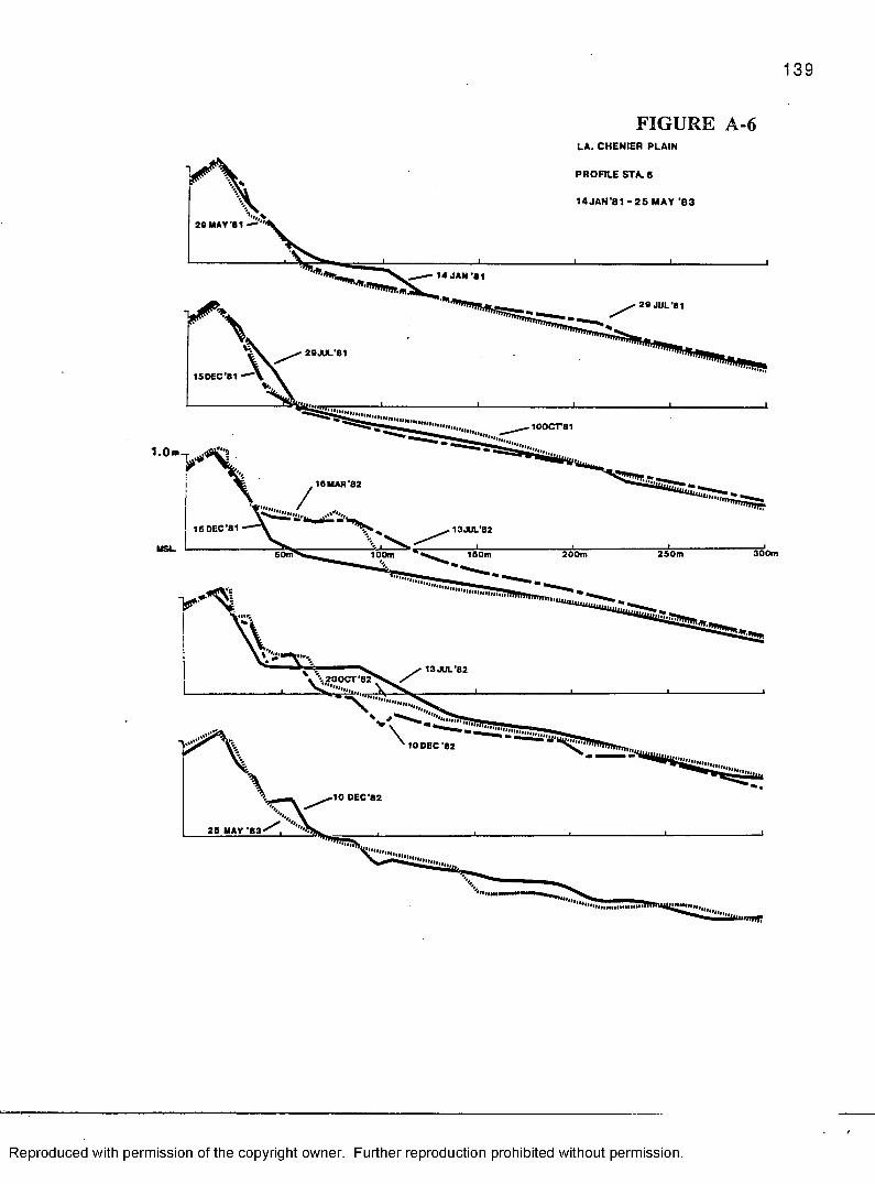
139
1 •On*
USL.
F IG U R E A-6LA. CHENIER PLAIN
PROFILE STA. 6
1 4 JAN '81 “ 2 5 MAY '8 3
20 MAY'81
14 JAN '81
15 DEC'81
.......... ....
15 DEC'81
300m250m150m 200m50nf 100m
i OOCT'8
10 DEC '82
10 DEC’82
lC s a s B ==,
Reproduced with permission of the copyright owner. Further reproduction prohibited without permission.
/

140
FIGURE A-7
LA. C H EN IER PLAIN
PROFILE ST A. 7
13 FEB’e i “26MAY’83
.'8115DEC81
13 OCT‘81
^ ....1.Qm
24 JUN '82
16 MAR *82
MSL 300r250m200m150m50nv 100m15 DEC *81
'" " " ••I I IM h i i IHIII
150EC *82
'{ I m m y ^ i y jM I M H I I H H l y 20 SEP '82H >H lll l lH H l ||n t „ )|
15 DEC'82
28 MAY'83
... .....
Reproduced with permission of the copyright owner. Further reproduction prohibited without permission.

141
1.0m
MSL
FIGURE A-8
LA. CHENIER PLAIN
PROFILE ST A. 8
13 FE B ’8 1 - 2 6 MAY'83
20 MAY '81
20 JUL '61
j? " " 11.....
\ 15DEC81130CT*81
23JUN '82
8 APfl *82
— i s o m — '« « .7 > 2 0 0 m^ -iLt.3 0 0 m250m
*""1111111 """•••liUlllllMMIliiimmnTTii
100m
23 JUN'82
15DEC82
• ’ M ill,26 MAY *63
15 DEC '82
Utu
Reproduced with permission of the copyright owner. Further reproduction prohibited without permission.
A PPE N D IX B
PROGRAM FOR GRANT-MADSEN BOUNDARY LAYER CLOSURE
The FORTRAN program listed on the next five pages was used to
perform the boundary layer closure referenced in the text. Documentation is
provided in the comments on the first 3 pages. References of the form "GM
EQ X" are to equations which appear in the journal article from which this
program was developed (Grant and Madsen 1979).
142
Reproduced with permission of the copyright owner. Further reproduction prohibited without permission.

C * PROGRAM (GMMODEL) *C * THIS PROGRAM PERFORMS GRANT-MADSEN(1979) CLOSURE FOR *C * WAVE-CURRENT BOUNDARY LAYER PROBLEM. ANGULAR DEVIATION *C * OF MEAN CURRENT FROM DIRECTION OF WAVE PROPAGATION PHICB)*C * IS ASSUMED FIXED AND MUST BE POSITIVE AND LESS THAN 90 *C * DEGREES. A NIKURADSE BOTTOM ROUGHNESS(XKB) MUST ALSO BE *C * SPECIFIED. INITIALLY, GUESS A VALUE FOR UA/UB(RATIO) AND*C * WAVE-CURRENT FRICTION FACTOR(FCW). OBTAIN A NEW VALUE *C * FOR FCW THROUGH ITERATION IN NESTED LOOP. RETURN TO MAIN*C * LOOP TO CALCULATE AN APPARENT BOTTOM ROUGHNESS(XKBC1) *C * WHICH IS COMPARED TO VALUE CALCULATED FROM FIELD DATA *C * (XKBC2) FOR MEAN CURRENT VELOCITY(UCR) MEASURED AT *C * REFERENCE ELEVATION(ZR) ABOVE BED. IF A SPECIFIED *C * TOLERANCE(TOL2) IS EXCEEDED, MAIN LOOP IS RE-EXECUTED *C * WITH AN ADJUSTED VALUE FOR UA/UB(RATIO). THIS PROCESS IS*C * REPEATED UNTIL CONVERGENCE CRITERION IS SATISFIED. *C ************************************************************C INPUTSC FIELD VALUES FOR WAVE CHARACTERISTICS(LINEAR WAVE THEORY)C TITLE RUN NO.C FREQ WAVE FREQUENCY IN RADSC UB MAX NEAR-BOTTOM ORBITAL VELOCITY(CM/S)C AB NEAR-BOTTOM OSCILLATORY EXCURSION AMP(CM)CCCCCCC FIELD VALUES FOR CURRENT CHARACTERISTICSC PHICB DEVIATION OF MEAN STRESS VECTOR FROM DIRECTION OFC WAVE PROPAGATION IN RADS(LESS THAN 90 DEG)C PHIC DEVIATION OF MEAN CURRENT IN WBL FROM DIRECTION OFC WAVE PROPAGATION IN RADS. GM EQ 18.C UCR MEAN CURRENT VELOCITY AT REFERENCE ELEVATION IN CM/SC ZR REFERENCE ELEVATION-POSITIVE UP IN CM.C XKB NIKURADSE ROUGHNESS IN CMCCCCCC TOLERANCES FOR ITERATIONSC TOL1 PERMISSABLE ERROR FOR FCW ITERATIONC TOL2 PERMISSABLE ERROR FOR KBC ITERATIONCCCCC VARIABLES FOR WHICH STARTING ESTIMATES ARE NEEDED C RATIO RATIO OF UNKNOWN CURRENT REFERENCE VELOCITY TO MAXC NEAR-BOTTOM ORBITAL VELOCITY (UA/AB). USE (UCR/AB)
Reproduced with permission of the copyright owner. Further reproduction prohibited without permission.

ccccccccccccccccccccccccccccccccc
TO START.FCW WAVE-CURRENT FRICTION FACTOR.
GM FIG.4.CHOOSE START VALUE FROM
CCCCCCCCCCCCC
VARIABLES FOR WHICH NO STARTING ESTIMATES ARE NEEDED VARIABLES DEPENDENT ON RATIO AND PHIC ONLY V2 GM EQ 16ALPHA GM EQ 20
TERMS DEPENDENT ON V2, ALPHA, AND PHICB ONLY Q1 LAST TERM LFT SIDE GM EQ 54Q2 RT SIDE GM EQ 54
TERMS CALCULATED IN FCW ITERATIONUCW CHARACTERISTIC TURBULENCE INTENSITY IN WBL(U*CW)
GM EQ 21XL PRANDTL MIXING LENGTH(L)
GM EQ 29ZETAO NO-SLIP WBL BOTTOM BOUNDARY PARAMETER
GM EQ 31X ARGUMENT OF KELVIN FUNCTION (2*SQRT(ZETAO))
TERMS CALCULATED IN IMSL SUBROUTINE MMKELOc BER BER X (ORDER 0)c BEI BEI X (ORDER 0)c XKER KER X (ORDER 0)c XKEI KEI X (ORDER 0)c IER ERROR PARAMETER
XK BRACED TERMS IN GM EQ 53GFCW NEW ESTIMATE OF FCW FROM TRANSPOSED GM EQ 54Q3 SECOND TERM LFT SIDE TRANSPOSED GM EQ 54Q4 DUMMY VARIABLE USED IN CALCULATING GFCWXDIF1 (GFCW - FCW)
Reproduced with permission of the copyright owner. Further reproduction prohibited without permission.

oo
oo
o
on
o
oo
oo
oo
oo TERMS DEPENDENT ON RESULTS OF FCW ITERATION
UC CHARACTERISTIC SHEAR VELOCITY ABOVE WBL GM EQ 15BETA EXPONENT IN GM EQ A9XKBC1 ESTIMATE OF XKBC FROM TRANSPOSED GM EQ A9XKBC2 FIELD BASED ESTIMATE OF XKBC FROM GM EQ 49XDIF2 XKBC2-XKBC1
DIMENSION TITLE(2)READ(5,10) TITLE,FREQ,UB,AB READ(5,20) PHICB,PHIC,UCR,ZR.XKB READ(5,20) T0L1.T0L2 READ(5,20) RATIO,FCW
10 F0RMAT(2A4,2X,3F10.5) _ .... - - -'20 F0RMAT(7F10.5)
WRITE(6,100) TITLE WRITE(6,200) FREQ,UB,AB WRITE(6,300) PHICB,PHIC,UCR,ZR,XKB WRITE(6,400) T0L1.T0L2 WRITE(6,500) RATIO,FCW
100 F0RMAT('1',2X,2A4,10X,’INITIAL VALUES')200 FORMATC'O',2X,'WAVE PARAMETERS’/2X,'FREQ =',F10.5,2X,'UB =',
1 F10.5,2X,'AB =',F10.5)300 F0RMAT('0',2X,'CURRENT PARAMETERS’/2X, 'PHICB =',F10.5,15X,
1 'PHIC ='.F10.5/2X,'UCR =',F10.5,2X,'ZR =',F10.5,2X,'XKB =',1 F10.5)
400 F0RMAT('0',2X,'CONVERGENCE TOLERANCES'/2X, 'FCW ITERATION*,F11.5/ 1 2X,'XKBC ITERATION',F10.5)
500 FORMATC'O',2X,'STARTING ESTIMATES'/2X,'RATIO'.F10.5/2X,'FCW',1 F12.5)
XKAPPA =0.4 PI =3.14159
30 DO 1 J = l , 21 C EXIT LOOP IF NO CONVERGENCE AFTER 20 ITERATIONS
I F ( J .EQ. 2 1 ) GO TO 210V2 = ( ( 2 . * R A T I 0 ) / P I ) * S Q R T ( 4 . - ( 3 . * ( S I N ( P H I C ) ) * * 2 . ) )ALPHA = 1 .+ (R A T I0**2 .)+2 .*R A T IO *C O S (P H IC )Q3 = ( ( ( SQRT(SQRT(ALPHA)) ) * * 3 . ) / 4 . ) - ( ( V 2**2 . ) / ( 4 . *SQRT(ALPHA)) )Q2 =(V2/(2 .*SQR T(SQ RT(A LPH A )) ) )*COS(PHICB)
W R IT E (6 ,6 0 0 ) J ,V 2,A LPH A ,Q 2,Q 3 600 F O R M A T ( ' l ' , 2 X , ’ TERMS DEPENDENT ON RATIO, PHIC, AND PHICB ONLY'/
1 2X,'ITERATION = ’ , I 3 / 2 X , 'V 2 = ' ,F 1 0 .5 /2 X , 'A L P H A = ' , F 1 0 . 5 / 2 X , ' Q2 = ' 1 F 1 0 . 5 , 2 X , ' Q3 = ' , F 1 0 . 5 )
Reproduced with permission of the copyright owner. Further reproduction prohibited without permission.

40 DO 2 K=1,21C EXIT LOOP IF NO CONVERGENCE AFTER 20 ITERATIONS.
IF(K .EQ. 21) GO TO 220UCW =SQRT(.5*FCW*ALPHA*UB**2.)
UC =SQRT(0.5*FCW*V2*(UB**2.))XL =(XKAPPA*UCW)/FREQ ZETAO =XKB/(30.*XL)X =2.*SQRT(ZETA0)WRITE(6,700) K,UCW,UC,XL,ZETAO,X CALL MMKELO CX,BER,BEI,XKER,XKEI,IER)WRITE(6,800) BER,BEI,XKER,XKEI,IER XKEI =ABS(XKEI)XK =1./(X*(SQRT((XKER**2.)+(XKEI**2. ))))Q1 =.097*SQRT(XKB/AB)*(XK/FCW**(3./4.))Q4 =XK* v Q.9J*SQRTCXKB./AB.)#( ( Ql+( 2 .*Q2 -) ) /Q3 )......-.......GFCW =(Q4**(4./3.))WRITEC6,900) FCW,GFCW,XK,Q1,Q2,Q3,Q4 XDIF1 =(GFCW-FCW)IF(ABS(XDIF1) .LE. T0L1) GO TO 50 FCW =GFCW
2 CONTINUE700 FORMATCl','TERMS USED IN MMKELO. ITER = ',I3/2X,'UCW =',F10.5,
1 2X,'UC =' ,F10.5/2X,1 XL =',F10.5,2X,'ZETAO =',F10.5,2X,'X 1 F10.5)
800 FORMATC'O',2X,'MMKELO OUTPUT1/2X,'BERX =',F10.5,2X,'BEIX =',1 F10.5/2X,'XKER =',F10.5,2X,'XKEI =',F10.5,2X,1IER =',F10.5)
900 FORMATC'O',2X,'FACTORS USED TO FIND GFCW'/2X,'FCW =',F10.5,2X,1 'GFCW =' ,F10.5,2X,'XK = ',F10.5/2X,'Q1 =',F10.5,2X,'Q2 1 F10.5,2X,'Q3 =',F10.5,2X,'Q4 =’,F10.5)
50 FCW =GFCWUC =SQRT(0.5*FCW*V2*CUB**2.))UCW =SQRTC.5*FCW*ALPHA*UB**2. )BETA =1.-(UC/UCW)WRITEC6,910) K,UC,UCW,BETA,FCW
910 FORMATC'1',2X,'CONVERGENCE REACHED ON FCW AFTER',13,1 ' ITERATIONS'/2X,'TERMS NEEDED TO FIND XKBC’/2X,'UC =',F10.5,1 'UCW =' ,F10.5,2X,'BETA =',F10.5,2X,'FCW =',F10.5)XKBC1 =XKB*CC24.*(UCW/UB)*(AB/XKB))**BETA)XKBC2 =30.*ZR/EXP(UCR*XKAPPA/UC)XDIF2 =XKBC2-XKBC1 WRITEC6,920) J,RATIO,XKBC1,XKBC2,XDIF2
920 FORMATC'O',2X,'RESULTS OF ITERATION',13,' ON KBC'/2X,'RATIO =', 1 F10.5,2X,'XKBC1 =',F10.5,2X,'XKBC2 =',F10.5,2X,'XDIF2 1 F10.5)IFCABSCXDIF2) .LE. T0L2) GO TO 60 IFCABSCXDIF2) .LE. 5.) GO TO 55 RATIO =RATI0*SQRTCXKBC1/XKBC2)GO TO 1
55 RATIO =RATI0*SQRT(SQRTCXKBC1/XKBC2))1 CONTINUE
210 WRITEC6,310)GO TO 999
220 WRITEC6,320)GO TO 999
Reproduced with permission of the copyright owner. Further reproduction prohibited without permission.

310 FORMATC' 1 ' , ' NO CONVERGENCE ON RATIO AFTER 20 ITERATIONS. ABORT') 320 FORMATC’ 1 NO CONVERGENCE ON FCW AFTER 20 ITERATIONS. ABORT')
60 XKBC =XKBC2W R ITE(6 ,9 3 0 ) J ,T IT L E
930 FORMATC'l',2X,'CONVERGENCE REACHED ON RATIO A F T E R ',13 ,1 1 IT E R A T IO N S '/2 X .2 A 4 ,1 0 X , ' INITIAL VALUES')WRITEC6.200) FREQ, UB, AB WRITEC6,3 0 0 ) PHICB,PHIC,UCR,ZR,XKB WRITEC6 , 4 0 0 ) T 0L 1 ,T 0L 2 WRITEC6,9 4 0 )WRITE C 6 , 9 5 0 ) RATI0 , FCW, XKBC, UCW, UC, XL, ZETAO, V 2, ALPHA
940 FORMATC'O1,2 2 X , 'F IN A L RESULTS').................950 FORMATC'O', ' RATIO = ' ,F 1 0 .5 ,2 X , 'F C W = ' ,F 1 0 .5 ,2 X , 'X K B C = ’ , F 1 0 . 5 /
1 2 X , ' UCW = ' , F 1 0 . 5 , 2 X , 'U C = ’ , F 1 0 . 5 / 2 X , ' XL = ' , F 1 0 . 5 ,1 2X,'ZETAO = ' . F 1 0 . 5 / 2 X , 'V 2 = ' ,F 1 0 . 5 , 2 X . ' ^ f H A = ' , F I 0 . 5 ) ............. .......
: • w. r_ : g gj g 'CONTI NT)E r - - ; ...... -...r - - - - -.....STOPEND
Reproduced with permission of the copyright owner. Further reproduction prohibited without permission.

V IT A
George Paul Kemp was bom on May 2,1954, in Port Jefferson, New
York. He graduated cum laude from Saint Paul's School in Garden City,
New York, in May, 1971. He enrolled in the Fisheries Science program at
Cornell University in Ithaca, New York, and received the B.S. degree in May
1975. Mr. Kemp began graduate studies later that year in the Department of
Marine Sciences at Louisiana State University. Following award of the M.S.
degree in May, 1978, he pursued his interest in estuarine geochemistry as a
Research Associate in the Department of Engineering Research, also at
L.S.U., through the fall o f 1979. He then re-entered the Department of
Marine Sciences to begin a graduate program in coastal sedimentology
through the Coastal Studies Institute. Mr. Kemp was awarded the Joseph
Lipsey, Sr., Scholarship in 1981, and spent 1984 in Washington, D.C., where
he served on the legislative staff of Senator Edward M. Kennedy as a Sea
Grant Congressional Fellow. Since returning to Louisiana, Mr. Kemp has
been employed by Groundwater Technology, Inc., in Mandeville. Mr. Kemp
is currently a candidate for the Ph.D. degree in the Department of Marine
Sciences.
148
Reproduced with permission of the copyright owner. Further reproduction prohibited without permission.

DOCTORAL EXAMINATION AND DISSERTATION REPORT
Candidate: G. Paul Kemp
Major Field: Marine S c ien ces
Title of Dissertation: MUD DEPOSITION AT THE SHOREFAGE: WAVE AND SEDIMENTDYNAMICS ON THE CHENIER PLAIN OF LOUISIANA
Approved:
Major Professor and .Chairman
Dean of the Graduatee School
EXAMINING COMMITTEE:
Date of Examination:
November 26, 1986
n"7—7*
Reproduced with permission of the copyright owner. Further reproduction prohibited without permission.