Deposition and Simulation of Sediment Transport in the ...DEPOSITION AND SIMULATION OF SEDIMENT TRANSPORT IN THE LOWER SUSQUEHANNA RIVER RESERVOIR SYSTEM by Robert A. Hainly, Lloyd

Deposition and Simulationof Sediment Transport

in the Lower Susquehanna River Reservoir System

by Robert A. Hainly, Lloyd A. Reed, Herbert N. Flippo, Jr, and Gary J. Barton

Water-Resources Investigations Report 95-4122

Prepared in cooperation with thePENNSYLVANIA DEPARTMENT OF ENVIRONMENTAL RESOURCES, BUREAU OF SOIL AND WATER CONSERAVATION

Lemoyne, Pennsylvania 1995

U.S. DEPARTMENT OF THE INTERIOR

BRUCE BABBITT, Secretary

U.S. GEOLOGICAL SURVEY

Gordon P. Eaton, Director

For additional information write to:

District ChiefU.S. Geological Survey840 Market StreetLemoyne, Pennsylvania 17043-1586

Copies of this report may be purchased from:

U.S. Geological SurveyEarth Science Information CenterOpen-File Reports SectionBox 25286, MS 517Denver Federal CenterDenver, Colorado 80225

CONTENTSPage

Abstract..................................................................................... 1

Introduction .................................................................................. 1Purpose and scope ...................................................................... 1Description of the study area...............................................................2

Description of the hydroelectric dams and reservoirs ..................................................2Safe Harbor Dam and Lake Clarke ..........................................................2Holtwood Dam and Lake Aldred ............................................................5Conowingo Dam and Conowingo Reservoir ...................................................6

Previous studies ..............................................................................6

Data-collection methods ........................................................................7Seismic-reflection survey..................................................................7Bottom material .........................................................................7

Deposition in the Lower Susquehanna River reservoir system...........................................9Lake Clarke ........................................................................... 10

Sediment distribution .............................................................. 10Sediment composition ............................................................. 12

Particle size and coal percentage............................................... 12Nutrients .................................................................. 12Metals.................................................................... 14

Lake Aldred ...........................................................................17Sediment distribution .............................................................. 17Sediment composition ............................................................. 17

Particle size and coal percentage............................................... 17Nutrients .................................................................. 17Metals.................................................................... 17

Conowingo Reservoir.................................................................... 19Sediment distribution .............................................................. 19Sediment composition ............................................................. 19

Particle size and coal percentage............................................... 19Nutrients .................................................................. 19Metals ....................................................................21

Effect of deposition on reservoir storage .....................................................21Lake Clarke......................................................................21Lake Aldred......................................................................21Conowingo Reservoir..............................................................25

Simulation of sediment transport in the reservoir system ..............................................27Description of the selected model ..........................................................27Application of model to reservoir system .....................................................28

Development.....................................................................28Calibration.......................................................................30Results .........................................................................34

Summary and conclusions......................................................................37

References cited .............................................................................38

ILLUSTRATIONSPage

Figures 1-8. Maps showing:

1. The Susquehanna River Basin ................................................ 3

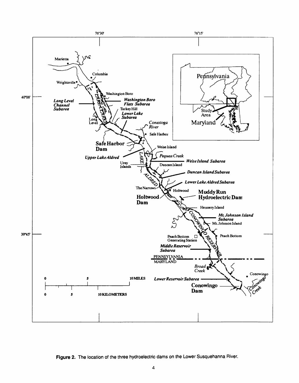
2. The location of the three hydroelectric dams on theLower Susquehanna River ............................................... 4

3. The thickness of sediment deposition in Lake Clarke.............................. 11

4. The percentage of clay in the sediment deposited in the three reservoirson the Lower Susquehanna River......................................... 13

5. Concentration ranges of organic nitrogen in the sediment deposited in the threereservoirs on the Lower Susquehanna River ................................ 15

6. Concentration ranges of phosphorus in the sediment deposited in the three reservoirson the Lower Susquehanna River......................................... 16

7. Concentration ranges of aluminum in the sediment deposited in the three reservoir?on the Lower Susquehanna River......................................... 18

8. The thickness of sediment deposition in Conowingo Reservoir ...................... 20

9-12. Graphs showing:

9. Water-storage capacity of Lake Clarke, Lower Susquehanna River Basin, from thetime the Safe Harbor Dam was completed in 1931 through 1990................. 22

10. Relations of upstream distance from Chesapeake Bay to average bed elevations and cross-sectional areas in Lake Clarke, Lower Susquehanna River Basin, 1931 and 1990 ............................ 23

11. Relations of upstream distance from Chesapeake Bay to average bed elevations and cross-sectional areas in Lake Aldred, Lower Susquehanna River Basin, 1910 and 1990 ............................ 24

12. Relations of upstream distance from Chesapeake Bay to average bed elevations and cross-sectional areas in Conowingo Reservoir, Lower Susquehanna River Basin, 1928,1959, and 1990....................... 26

TABLESPage

Table 1. Physical characteristics of the three hydroelectric darns and reservoirs on theLower Susquehanna River..................................................... 2

2. Physical characteristics of the Lower Susquehanna River reservoir subareas ................. 5

3. Site identification number and location of water-quality and bottom-materialsampling sites on the Susquehanna River......................................... 8

4. Estimated sediment deposition and composition for subareas of and forLake Clarke, Lake Aldred, and Conowlngo Reservoir, 1990 .......................... 10

5. Mean concentrations and deposition of ammonia, organic nitrogen, phosphorus, iron, aluminum, and manganese in subareas of and in Lake Clarke, Lake Aldred, and Conowingo Reservoir.......................................... 12

6. Initial estimates of fractional distributions of particle loads for selected dischargesof the Susquehanna River at Marietta, Pa. ....................................... 29

7. Initial estimates of fractional distributions of particle loads for selecteddischarges of the Conestoga River and Pequea Creek Basins........................ 30

8. Original and revised fractional distributions of particle loads for selecteddischarges of the Susquehanna River at Marietta, Pa. .............................. 32

9. Original and revised fractional distributions of particle loads for selecteddischarges of the Conestoga River and Pequea Creek Basins........................ 33

10. Summary output from the HEC-6 model showing bed-surface and water-surface elevation change, the modeled discharge, and the sediment load passing each cross-section, in the Lower Susquehanna River reservoir system, December 30-31,1987....................................................... 35

11. Summary output from HEC-6 model calibration run showing 1987 sediment load introduced to each reservoir on the Susquehanna River and sediment load trap efficiency.......................................................... 36

12. Loads and trap efficiencies for the three-reservoir system on theLower Susquehanna River, as computed by the HEC-6 and Conn models,and by a hand integration method............................................... 36

13. HEC-6 loads and trap efficiencies for the three-reservoir system on theLower Susquehanna River, May and June 1972 ................................... 36

CONVERSION FACTORS AND ABBREVIATIONS

Multiply

inch (in.) foot (ft) mile (mi)

By.

Length25.4

0.30481.609

To obtain

millimetermeterkilometer

square foot (ft2) square mile (mi2) acre

Area

0.092942.5900.4047

square meter square kilometer hectare

foot per second (ft/s) mile per year (mi/year)

Velocity

0.30481.609

meter per second kilometer per year

cubic foot (ft3) acre-foot (acre-ft)

Volume

0.028321,233

cubic meter cubic meter

cubic foot per second

Flow

0.02832 cubic meter per second

ton, short

Mass

0.9072 megagram

degree Fahrenheit (°F)

Temperature °C - 5/9 x (°F-32) degree Celsius

pounds per square foot (Ib/ft2)

Pressure

0.04788 dynes per square rmter

pounds per cubic foot (Ib/ft3)

Density

16.02 kilograms per cubic meter

Sea level: In this report "sea level" refers to the National Geodetic Vertical Datum of 192P (NVGD of 1929) a geodetic datum derived from a general adjustment of the first-order level nets o^both the United States and Canada, formerly called Sea Level Datum of 1929.

vi

DEPOSITION AND SIMULATION OF SEDIMENT TRANSPORT IN THE LOWER SUSQUEHANNA RIVER RESERVOIR SYSTEM

by Robert A. Hainly, Lloyd A. Reed, Herbert N. Flippo, Jr., and Gary J. Barton

ABSTRACT

The Susquehanna River drains 27,510 square miles in New York, Pennsylvania, and Maryland and is the largest tributary to the Chesapeake Bay. Three large hydroelectric dams are located on the river, Safe Harbor (Lake Clarice) and Holtwood (Lake Aldred) in southern Pennsylvania, and Conowingo (Conowingo Reservoir) in northern Maryland. About 259 million tons of sediment have been deposited in the three reservoirs. Lake Clarke contains about 90.7 million tons of sediment, Lake Aldred contains about 13.6 million tons, and Conowingo Reservoir contains about 155 million tons. An estimated 64.8 million tons of sand, 19.7 million tons of coal, 112 million tons of silt, and 63.3 million tons of clay are deposited in the three reservoirs. Deposition in the reservoirs is variable and ranges from 0 to 30 feet.

Chemical analyses of sediment core samples indicate that the three reservoirs combined contain about 814,000 tons of organic nitrogen, 98,900 tons of ammonia as nitrogen, 226,000 tons of phosphorus, 5,610,000 tons of iron, 2,250,000 tons of aluminum, and about 409,000 tons of manganese.

Historical data indicate that Lake Clarke and Lake Aldred have reached equilibrium, and that they no longer store sediment. A comparison of cross-sectional data from Lake Clarke and Lake Aldred with data from Conowingo Reservoir indicates that Conowingo Reservoir will reach equilibrium within the next 20 to 30 years. As the Conowingo Reservoir fills with sediment and approaches equilibrium, the amount of sediment transported to the Chesapeake Bay will increase. The most notable increase will take place when very high flows scour the deposited sediment.

Sediment transport through the reservoir system was simulated with the U.S. Army Corps of Engineers' HEC-6 computer model. The model was calibrated with monthly sediment loads fo- calendar year 1987. Calibration runs with options set for maximum trap efficiency and a "natural" particle-size distribution resulted in an overall computed trap efficiency of 34 percent for 1987, much less th=m the measured efficiency of 71 percent.

INTRODUCTION

The District of Columbia and the States of Pennsylvania, Maryland, and Virginia have agreed to a 40-percent reduction in controllable nutrient loads to the Chesapeake Bay by the year 2000. The load of nutrients transported to the bay depends, in large part, on the load transported by the Susquehanna River, the largest freshwater contributor to the bay. The reservoir system on the Lower Susquehanna R'ver affects the loads of sediment and nutrients delivered to Chesapeake Bay, but the magnitude and length of the effects are not known.

As part of the Chesapeake Bay Program, the Bureau of Land and Water Conservation of the Pennsylvania Department of Environmental Resources and the U.S. Geological Survey (USGS) cooperated in a study to evaluate deposition of sediment, nutrients, and selected metals in the three reservoirs on the Lower Susquehanna River. The study was conducted during the summer and fall of 1990.

Purpose and Scope

The quantity and chemistry of sediment in the reservoirs formed by the Safe Harbor, Holtwood, and Conowingo hydroelectric dams is evaluated in the report. The report presents a comparison of historical reservoir-bed elevations with elevations obtained during this study, and an estimate of the rem aining sediment storage capacity. The results of calibrating a model to calculate deposition and scour in the reservoirs during storms also are presented.

Data from the seismic-reflection profiling, data obtained during the collection of core semples, and historical data (Whaley, 1960) were used to map the thickness of bed sediments. The dry density and composition data determined from the core sample analyses, and the sediment thickness data were used to compute the dry weight and composition of the deposited material in each reservoir.

Description of the Study Area

The Susquehanna River drains 27,510 mi2 in south<entral New York, central Pennsylvania, and a small part of Maryland before entering the Chesapeake Bay (fig. 1). The reservoirs in the lower part of the Susquehanna drainage were formed by the construction of three hydroelectric dams on the 32-mi reach of the river between Conowingo, Md., and Columbia, Pa. (fig. 2). Conowingo Dam is in northern Maryland and forms Conowingo Reservoir, which extends into southern Pennsylvania. Holtwood Dam is upstream from Conowingo Reservoir and forms Lake Aldred. Safe Harbor Dam is upstream from Lake Aldred and forms Lake Clarke.

The climate in the Susquehanna River Basin varies considerably from central New Yorl State to northern Maryland. The mean annual temperature ranges from 45°F in central New York to 53°F in Maryland. The mean growing season ranges from 120 days in the north to 160 days in the sor*h (U.S. Department of Commerce, 1990). Mean annual precipitation in the basin is about 40 in. and is fairly evenly distributed throughout the year. The mean annual precipitation is highest in the lower basin and lowest in the headwaters.

Woodland covers 63 percent of the Susquehanna River Basin and is concentrated in the northern and western parts of the basin. Nineteen percent of the basin is tilled cropland, and most of the tiT«d cropland is in the lower basin. Extensive, cultivated areas are also along the river valleys in southern NTW York and northern Pennsylvania. Urban land occupies slightly more than 9 percent of the basin. Most cf the urban areas are along river valleys in southern New York and central Pennsylvania.

Anthracite coal was mined in several areas of eastern Pennsylvania. Fine coal from processing plants in the mining region was a large component of the sediment transported by the Susquehanna River from the late 19th century through the early 20th century, and "river coal" was routinely dredged f-om pools in the river until 1972. After the hydroelectric dams were constructed on the Lower Susquehanna River, large amounts of fine coal were trapped in the reservoirs.

DESCRIPTION OF THE HYDROELECTRIC DAMS AND RESERVOIRS

Safe Harbor Dam and Laks Clarks

Safe Harbor Dam, constructed in 1931, is 32 mi upstream from Chesapeake Bay (fig. 2). Lake Clarke extends upstream about 9.5 mi from Safe Harbor, Pa., to Columbia, Pa., and has a design capacity of 150,000 acre-ft (table 1). Streamflow in excess of plant capacity is regulated by flood gates along the top of the dam west of the hydroelectric plant.

Table 1. Physical characteristics of the three hydroelectric dams and reservoirs on the Lower Susquehanna River

Dam

Safe Harbor Holtwood Conowingo

Lake or reservoir

Clarke Aldred Conowingo

Year completed

1931 1910 1928

Elevation (feet above sea level)

Normal pool

227

1 170

109

Flood pool

227

180

109

Designcapacity

(acre-feet)

150,000 60,000

300,000

Surface area

(square miles)

9.5 4.0

12.8

b'^ximum turbine

d'«charge (cubic feet

pe r second)

110,000 27,000 81,000

1 Includes 4.75-foot flash boards.

79" 78' 77' 76' 75'

42 «

41°

40'

I

PENNSYLVANIA

25I

50 MILES I

I 25 SO KILOMETERS

EXPLANATION

~ Drainage basir boundary

State boundar'

Hydroelectric dams

Municipality

Figure 1. The Susquehanna River Basin.

76-301 76'15'

Marietta

4<T08'Long LevelChannelSubarea

39-451

Washington Boro

Washington Boro Flats Subarea

TiirkeyHill Lower Lake Subarea

( Conestoga * River

Safe Harbor Dam

Upper LakeAldred

Peach Bottom Generating Station

Middle Reservoir Subarea

PENNSYLVANIA MARYLAND

Weise Island Subarea

Duncan Island Subarea

Lower Lake A Idred Subarea

Muddy Run Hydroelectric Dam

Hennery Island

Mt. Johnson Island Subarea

ML Johnson Island

10 MILES Lower Reservoir Subarea Conowingo

'

10 KILOMETERS

Conowingo Dam

Figure 2. The location of the three hydroelectric dams on the Lower Susquehanna River.

4

For the purposes of this study, Lake Clarke was divided into three subareas the Washington Boro flats, the Long Level channel, and the lower lake (fig. 2, table 2). The Washington Boro flats are along the eastern half of the lake from Washington Boro to Turkey Hill. The surface area, excluding the thr?e large islands, is 2.7 mi2. Lake Clarke contains many small islands with land surfaces just above the normal water level and numerous sand and coal bars with surfaces just below the normal water level. Many sand and coal bars are exposed during low water and much of the area is too shallow for boating. The Long Level channel extends along the west side of the lake from about 3 mi upstream of the community of Long Level downstream to Turkey Hill. The surface area of the Long Level channel is 3.8 mi2 . The lower lake extends from Turkey Hill to the Safe Harbor Dam and has a surface area of 3.0 mi2.

Table 2. Physical characteristics of the Lower Susquehanna River reservoir subareas

Surface areaReservoir subarea (square

miles) (acres)

Channel length (feet)

Maximum width (feet)

Minimum width (feet)

Lake Clarke

Washington Boro FlatsLong Level channelLower Lake

Total

2.73.83.09.5

1,7202,4401,9306,090

24,60026,60022,400

^9,000

4,6806,6005,0008,840

8003,7203,0003,000

Lake Aldred

Upper Lake AldredWeise IslandDuncan IslandLower Lake Aldred

Total

1.21.01.3

.54.0

780660830290

2360

9,20013,00014,0006,400

42,600

5,0803,8002,7002,8005,080

4,0402,0001,2001,2001,200

Conowinpo Reservoir

Below Holtwood DamMt. Johnson IslandMiddle Reservoir areaLower Reservoir area

Total

1.53.64.73.0

12.8

9902,3103,0201,8908,210

17,20016,60023,32020,44077360

5,1606,8407,00053007,000

1,8405,12053003,1001,840

1 The total channel length is the sum of the Long Level channel and Lower Lake subareas because the Washington Boro flats and the Long Level channel are side-by-side, and not consecutive subareas.

Holtwood Dam and Lake Aldred

The Holtwood Dam, constructed in 1910, is about 25 mi upstream of Chesapeake Bay (fig. 2). The reservoir formed by the dam, Lake Aldred, extends upstream for about 8 mi. Lake Aldred covers an area of about 4.0 mi2 and has a design capacity of 60,000 acre-ft (table 1). Holtwood Dam was constructed without flood gates, and river flow in excess of plant capacity spills over the top of the dam to th? west of the powerhouse. A coal-fired power plant was constructed adjacent to the hydroelectric plant in 1925. The coal plant had a capacity of 73,000 kilowatts and was designed to burn about 200,000 tons of river coal per year. Until 1972, most of this coal was dredged from the reservoirs.

For this report, Lake Aldred was divided into four subareas (fig. 2, table 2). The most upstream subarea, Upper Lake Aldred, extends from the Safe Harbor Dam to Weise Island and covers 1.2 mi 2. The Weise Island subarea extends from Weise Island to just below the Urey Islands. This subarea of the lake is 13,000 ft long, and the width ranges from 3,800 ft just below Weise Island to 2,000 ft at the Urpv Islands. The surface area, not including Weise Island, is 1.0 mi 2. The Duncan Island subarea extends from just below the Urey Islands to the narrows. It is 14,000 ft long, and the width ranges from 2,700 ft above Duncan Island to 1,200 ft at the Narrows. The surface area is 1.3 mi2. Lower Lake Aldred extends from the Narrows to the dam. The width of this subarea ranges from 1,200 ft at the Narrows to 2,800 ft above the dam. The surface area is 0.5 mi2.

Conowingo Dam and Conowingo Reservoir

Conowingo Dam, constructed in 1928 about 10 mi upstream of Chesapeake Bay, is the largest hydroelectric dam and creates the largest reservoir on the river. Conowingo Reservoir has a surface area of 12.8 mi2 and a design capacity of 300,000 acre-ft (table 1). The elevation of the river bed at the dam is about 11 ft above sea level, and the normal pool elevation is 109 ft. River flow in excess of the plant capacity is discharged through flood gates installed on the east side of the dam.

Conowingo Reservoir extends about 12 mi from the dam upstream to Hennery Island (fig. 2). A 3.2-mi section of the river separates the Holtwood Dam from the headwaters of the Conowingo Reservoir at Hennery Island. Water velocities in this river section are high, and sediment does not accumulate. The remainder of the reservoir was divided into three subareas the Mt. Johnson Island subarea, the Middle Reservoir subarea, and the Lower Reservoir subarea (table 2).

The Mt. Johnson Island subarea extends from Hennery Island to just below the Peach Bottom Generating Station and has an average width of about 6,000 ft. The surface area is 3.6 mi2. The Middle Reservoir subarea extends from below the Peach Bottom Generating Station to Broad Creek. The width of the Middle Reservoir subarea ranges from 7,000 ft just below the Peach Bottom Generating Sftion to 5,500 ft at Broad Creek, and the surface area is 4.7 mi2. The Lower Reservoir subarea extends from Broad Creek to Conowingo Dam. The width of this subarea ranges from 5,500 ft at Broad Creek to 3,100 ft at Conowingo Creek and increases to about 4,900 ft at the dam. The surface area of the Lower Reservoir subarea is 3.0 mi2.

PREVIOUS STUDIES

Anthracite coal was a major component of the sediment transported by the Susquehanm River from the late 19th century through the early 20th century. Mined coal was brought to the land surface, broken, and washed. At many of the coal-processing areas, the waste water from the washing operations was discharged directly to streams. An estimated 10-15 percent of the coal that was mined and run through the breakers was discharged in the wash water. Sisler and others (1928) reported that 260,000 tons of coal were dredged from the Susquehanna River in 1913 and that half of that amount had a diameter larger than 2 mm (millimeters). They also reported that continuing deposition and scour were moving a large coal bar down the river at a rate of about 3 mi per year. By 1925, dredge operators were recovering 400,000 tons of coal a year from the Susquehanna River.

Schuleen and Higgins (1953) reported the results of siltation surveys in Lake Clarke. They reported that Lake Clarke contained 144,600 acre-ft of water in 1931, and the capacity was reduced to 78,800 acre-ft in 1950. The implication is that nearly 66,000 acre-ft of water storage (about 45 percent of the design capacity) was lost because of sediment deposition during 1931-50. In 20 years, the lake trapped about 74 million tons of sediment, which is an average deposition rate of 3.7 million tons per year. Surveys completed in 1950,1951,1959, and 1964 indicated that the amount of sediment in Lake Clarke remained fairly constant at 74 million tons from 1950 to 1964 and that the reservoir had reached an equilibrium (E.T. Schuleen, Pennsylvania Power and Light Company, oral commun., 1965).

Schuleen and Higgins (1953) also collected suspended-sediment data from the Susquehenna River at Columbia and at Safe Harbor during 1948-53. During the 6-year period, sediment discharge a* Columbia, upstream of Lake Clarke, averaged 4.46 million tons per year and the sediment discharge measured at Safe Harbor, the outflow of the reservoir, was 3.13 million tons per year.

Levin and Smith (1954) reported on a river-coal dredging operation in Lake Clarke that started in 1953. The operation was designed to dredge 1 million tons of material a year from Lake Clarke rnd transport it on barges to the shore where the sand and coal were separated. The dredged material was about half sand and half coal. Dredging continued until the flood caused by Hurricane Agnes in June 1972. Because the reservoir surveys conducted in 1951,1959, and 1961 indicated the amount of sediment deposited in Lake Clarke remained about the same, the dredged material was replaced by incoming sediments.

Ledvina (1962) reported results of siltation surveys of Lake Aldred conducted by the Penrsylvania Power and Light Company and the Holtwood Steam Electric Station. These surveys indicate thet the annual amounts of sediment deposited in Lake Aldred are variable. Ledvina reported that the lake contained 19.3 million tons of sediment in 1939,13.3 million tons in 1950, and 9.97 million tons in 1961. Reasons for the decline in sediment were not given, but coal was dredged from the reservoir du~ing most of the period.

Whaley (1960) reported temperature, dissolved oxygen concentrations, velocity distributions, and bottom elevations at six cross-sections in Conowingo Reservoir in 1959. His data indicate that thr? capacity of Conowingo Reservoir was reduced from 300,000 acre-ft in 1928 to 235,000 acre-ft in 1959. The reservoir contained an estimated 92 million tons of sediment in 1959.

DATA-COLLECTION METHODS

Continuous seismic-reflection profiles were run at about 10 locations in each of the lakes to determine the areal extent and the thickness of sediment deposition. Bottom-material sampling points were selected to characterize the particle size and chemistry of the material deposited in the reservoirs and to confirm the sediment thickness as determined by geophysical techniques. Suspended-sediment samples were collected during periods of high flow from 1984 to 1989 at the Susquehanna River at Marie'te, Pa., and from the Conestoga River at Conestoga, Pa. The sediment deposition data were used, along with suspended-sediment transport data, to calibrate and test a model to compute deposition and re- suspension of sediment over a range of flows.

Seismic-Reflection Survey

The continuous seismic-reflection profiling method (Gorin and Haeni, 1988; Wolansky and others, 1982) is based on signals transmitted from a sound source and reflected at air-water, water-sediment, and sediment-rock interfaces. Depths are determined by observing the arrival time of the reflected waves and applying a velocity to the wave. The velocity of sound is related to compressibility and specific veight of the medium through which it travels. The velocity of sound in water is 4,720 ft/s and the velocit" in saturated unconsolidated sediments is about 5,000 ft/s. The velocity of sound in bedrock varies 1 -it is also greater than velocity of sound in water. The seismic signal penetrates to a depth of 100 ft in fine-<?rained sediments but is limited to 5 ft in coarse sediments because gravel and larger particles severely scatter the signals. Resolution is 1 to 2 ft. A fathometer, operating at a signal frequency of 192 kilohertz, was also used to provide a record of water depth and morphology of the bottom of each reservoir.

Bottom Material

A total of 54 core samples were collected from the bottom material in the reservoirs from October 1990 to April 1991. The sample-collection sites in each reservoir are listed in table 3. Samples of tt « bottom material were collected to a maximum depth of 7 ft with a 2-in. diameter stainless-steel core sampler equipped with a plastic liner. Bed-material samples were analyzed for particle-size distribution, percentage of coal, dry density, and concentrations of selected nutrient and metal species. Result' of all sample analyses are published in "Water Resources Data for Pennsylvania, Water Year 1991, Volume 2" (Durlin and Schaffstall, 1992).

Table 3. Site identification number and location of water-quality and bottom-material sampling site~ on the Lower Susquehanna River

[Latitude, in degrees, minutes, seconds north; Longitude in degrees, minutes, seconds west]

Lake Clarke

Site number

LC 05.01LC 05.06

LC 07.02

LC 07.03

LC 09.03

LC 10.01

LC 10.02

LC 10.03

LC 10.04

LC 12.01

LC 12.03

LC 12.05

LC 12.07

LC 14.07

LC 14.09

LC 14.10

LC 15.02

LC 15.06

LC 16.03

Latitude

395738395757

395624

395635

395538

395457

395518

395529

395542

395756

395822

395904

395931

395701

395620

395550

395550

395627

395546

Longitude

07629080762755

0762704

0762653

0762501

0762417

0762405

0762358

0762355

0762728

0762738

0762801

0762819

0762754

0762640

0762517

0762603

0762728

0762433

Lake Aldred

Site number

LA 01.02LA 03.02

LA 03.04

LA 04.02

LA 04.03

LA 06.02

LA 06.03

LA 12.03

LA 12.11

LA 12.14

LA 12.18

LA 13.09

LA 13.11

LA 13.12

LA 15.04

LA 15.06

LA 15.13

LA 15.14

LA 16.03

LA 16.05

LA 17.03

LA 17.04

LA 17.07

LA 17.09

LA 17.11

Latitude

394947395050

395058

395127

395135

395303

395305

395414

395210

395111

394944

395023

395040

395050

394958

395015

395132

395142

395329

395353

395341

395320

395244

395220

395155

Longitude

0762008

0762101

0762045

0762133

0762125

0762219

0762231

0762241

0762226

0762108

0762023

0762057

0762059

0762105

0762035

0762047

0762158

0762218

0762247

0762254

0762219

0762218

0762254

0762248

0762234

Conowingo Reservoir

Site number

CO 01.01CO 01.03CO 01.05

CO 02.02

CO 02.03

CO 02.04

CO 03.05

CO 04.03

CO 04.05

CO 05.02

CO 07.03

CO 08.01

CO 08.03

CO 08.05

CO 09.02

CO 09.03

CO 10.03

CO 11. 06

CO 12.01

CO 12.05

CO 12.06

CO 13.02

CO 13.05

Latitude

393939393955

394010

394039

394025

394017

394104

394208

394212

394254

394453

394608

394544

394524

394704

394655

394738

394530

394339

394148

394126

394107

394007

Longitude

0761109

0761058

0761049

0761150

0761152

0761200

0761255

0761402

0761335

0761407

0761441

0761508

0761523

0761545

0761605

0761622

0761716

0761430

0761407

0761318

0761258

0761223

0761124

All chemical analyses were performed at the USGS National Water Quality Laboratory in Arvada, Colo. Bed-material particle-size analyses were performed at the USGS Pennsylvania District Sediment Laboratory in Lemoyne to determine the percentage of sand, silt, clay, and coal. Samples of the bottom material were sieved to determine the weight of sediment that had a diameter of greater than 0.062,0.125, 025, 0.50,1.00, and 2.00 mm. The percentages of silt and clay were determined by standard particle-size analysis techniques (Guy, 1969).

The percentage of coal by volume of each of the six sieved portions was visually estimated. and then used to estimate the percentage of coal and sand by weight in each sample. The following example demonstrates the method used to determine the percentages of sand and coal by weight in each sieved portion of the sediment samples.

A 0.89 g portion of sediment in the 1.00-2.00 mm class was visually estimated to contain 4^ percent coal and 60 percent sand, by volume. Specific gravities of 1.7 for coal and 2.4 for sand were assumed. The relative weights of coal and sand were determined by multiplying the volume estimate by the assumed specific gravity for each particle type.

0.40 x 1.7 = 0.68 (relative weight of coal in this portion) (1)

0.60 x 2.4 = 1.44 (relative weight of sand in this portion) (2)

0.68 + 1.44 = 2.12 (total relative weight) (3)

To determine the actual weight of coal and sand in the portion, the ratio of the total actual weight of the sample and the total relative weight was determined.

0.89 g / 2.12 = 0.42 (ratio of total actual weight to total relative weight) (4)

The ratio was then multiplied by the relative weights to determine the actual weight of ccal and sand in the portion.

0.68 x 0.42 = 0.29 g (weight of coal in this portion) (5)

1.44 x 0.42 = 0.60 g (weight of sand in this portion) (6)

The percentages of coal and sand, by weight, in this 1.00-2.00 mm class portion are 33 percent (0.29 g / 0.89 g) and 67 percent (0.60 g / 0.89 g), respectively.

DEPOSITION IN THE LOWER SUSQUEHANNA RIVER RESERVOIR SYSTE"

After the hydroelectric dams were constructed on the Lower Susquehanna River, large amounts of coal and other sand-size particles and some of the silt and clay particles transported by the river were trapped in the reservoirs and no longer reached Chesapeake Bay. The headwaters of the reserve irs generally contain large deposits of sand and coal and the middle and lower parts of the reservoirs contain less sand and coal and more silt and clay.

About 10 percent of the nitrogen trapped in the sediments is ammonia and the rest is organic nitrogen. Together, nitrite and nitrate accounted for less than 0.1 percent of the total nitrogen in each of the impoundments and are not discussed in this report. For this report, concentrations of ammonia and organic nitrogen are expressed as nitrogen (N) and concentrations of phosphorus are expressed as phosphorus (P).

Data from bed-material samples from each of the three impoundments indicated that concentrations of iron were generally 2 to 3 times greater than concentrations of aluminum and 12 to 18 times greater than concentrations of manganese.

Lake Clarke

Sediment Distribution

Sediment deposition in Lake Clarke was greatest in the Lower Lake area and least in the Long Level channel (fig. 3, table 4). The Washington Boro flats, excluding the three large islands, contained about 15,600 acre-ft (723 million ft3) of sediment. Sediment samples collected in the Washington Boro flats had a dry density of about 71 Ib/ft3, and about 25.7 million tons of sediment were deposited in the fhts (table 4). The upstream 3 mi of the bed of the Long Level channel is composed primarily of cobbles ancf boulders (material with a diameter greater than 64 mm), and few (if any) deposits of fine-grained sediment are present. Sediment deposited in the 520-acre downstream reach of the Long Level channel, from Long Level to Turkey Hill, has an average depth of 3.7 ft, and the area contains about 1,920 acre-ft o* sediment (table 4)

The amount of sediment deposited in the Lower Lake subarea of Lake Clarke is about 43,600 acre-ft (1.9 billion ft3); the density of the sediment is about 65 Ib/ft3, the weight of sediment is calculated to be about 62.0 million tons (table 4). The total weight of sediment in Lake Clarke is about 90.7 miFon tons..

Table 4. Estimated sediment deposition and composition for subareas of and for Lake Clarke, Lake Ald'-vi, and Conowingo Reservoir, Lower Susquehanna River Basin, 1990

Reservoir or Reservoir subarea

Design capacity Sediment deposition(acre-feet) (acre-feet) (tons)

Sand (percent)

Silt (percent)

Clay (percent)

Coal (percent)

Lake Clarke

Washington Boro flats Long Level channel Lower Lake

Lake Clarke

24,600 47,600 77,800

150,000

15,600 1,920

43,60061,120

25,700,000 3,000,000

62,000,000

90,700,000

52 26 1828

16 43 49

39

10 30 2823

22 1 5

10

Lake Aldred

Weise IslandDuncan IslandLower Lake Aldred

Lake Aldred

4,70019,50020,50060,000

4,1303,2801,1708,580

6,600,0005,200,0001,800,000

13,600,000

33463138

35212829

15212118

16122015

Conowinpo Reservoir

Mt Johnson IslandMiddle ReservoirLower Reservoir

Conowingo Reservoir

41,000114,000145,000300,000

7,12041,100

56,700104,920

11,000,00063,400,00080,500,000

155,000,000

4539

522

1836

5846

7183526

307

26

10

4CT08'

39-351

Wrightsville*

Washington Boro

0

EXPLANATION Thickness of sediment deposition, in feet.

% Less Than 10

3 10 To 20

8 Greater Than 20

Safe Harbor

Safe Harbor Dam

SMILES

0 5 KILOMETERS

Figure 3. The thickness of sediment deposition in Lake Clarke.

11

Sediment Composition

Particle size and coal percentages

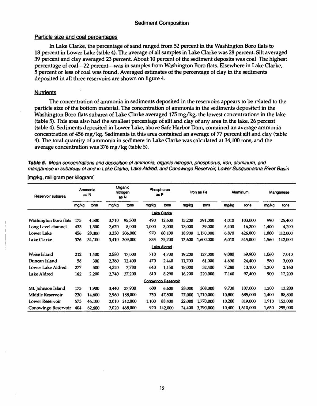
In Lake Clarke, the percentage of sand ranged from 52 percent in the Washington Boro flats to 18 percent in Lower Lake (table 4). The average of all samples in Lake Clarke was 28 percent. Silt averaged 39 percent and clay averaged 23 percent. About 10 percent of the sediment deposits was coal. The highest percentage of coal 22 percent was in samples from Washington Boro flats. Elsewhere in Lake Clarke, 5 percent or less of coal was found. Averaged estimates of the percentage of clay in the sediments deposited in all three reservoirs are shown on figure 4.

Nutrients

The concentration of ammonia in sediments deposited in the reservoirs appears to be related to the particle size of the bottom material. The concentration of ammonia in the sediments deposite-i in the Washington Boro flats subarea of Lake Clarke averaged 175 mg/kg, the lowest concentration-' in the lake (table 5). This area also had the smallest percentage of silt and clay of any area in the lake, 26 percent (table 4). Sediments deposited in Lower Lake, above Safe Harbor Dam, contained an average ammonia concentration of 456 mg/kg. Sediments in this area contained an average of 77 percent silt and clay (table 4). The total quantity of ammonia in sediment in Lake Clarke was calculated at 34,100 tons, and the average concentration was 376 mg/kg (table 5).

Table 5. Mean concentrations and deposition of ammonia, organic nitrogen, phosphorus, iron, aluminum, and manganese in subareas of and in Lake Clarke, Lake Aldred, and Conowingo Reservoir, Lower Susquehanna River Basin

[mg/kg, milligram per kilogram]

Ammonia Reservoir subarea M N

mg/kg tons

Organic nitrogen

asN

mg/kg tons

Phosphorus asP

mg/kg tons

Iron as Fe

mg/kg tons

Aluminum

mg/kg tons

Manganese

mg/kg tons

Lake Clarke

Washington Boro flats 175Long Level channel 433Lower Lake 456Lake Clarke 376

4,5001,300

28,30034,100

3,7102,6703,3303,410

95,3008,000

206,000309,000

4901,000

970835

12,6003,000

60,10075,700

15,20013,00018,90017,600

391,00039,000

1,170,0001,600,000

4,0105,4006,8706,010

103,00016,200

426,000545,000

9901,4001,8001,560

25,4004,200

112,000142,000

LakeAkfrod

Weise Island 212Duncan Island 58Lower Lake Aldred 277Lake Aldred 162

1,400300500

2,200

238023804,3202,740

17,00012,4007,780

37,200

710470640610

4,7002,4401,1508,290

19,20011,70018,00016,200

127,00061,00032,400

220,000

9,0804,6907,2807,160

59,90024,40013,10097,400

1,060580

1,200900

7,0103,0002,160

12,200

Conowinqo Reservoir

Mt Johnson Island 173Middle Reservoir 230Lower Reservoir 573Conowingo Reservoir 404

1,90014,60046,10062,600

3,4402,9603,0103,020

37,900188,000242,000468,000

600750

1,100920

6,60047,50088,400

142,000

28,00027,00022,00024,400

308,0001,710,0001,770,0003,790,000

9,73010,80010,20010,400

107,000685,000819,000

1,610,000

1,2001,4001,9101,650

13,20088,800

153,000255,000

12

76'IS1

4V08

\» Safe Harbor ,S«J» Harbor

39*45*Peach Bottom D Generating Station


EXPLANATION Percent clay in depositedsediment.

j LessThanIO

] 10To20

\ 20To30

3 30To40

Hennery Island

10MILES

J

Conowingo

10KILOMETCRS Conowingo OaniN

Rgure 4. The percentage of day in the sediment deposited in the three reservoirs on the Lower Susquehanna River.

13

Ranges of concentrations of organic nitrogen in the sediments deposited in all three reservoirs are shown in figure 5. Lake Clarke contained 309,000 tons of organic nitrogen, and the average concentration was 3,410 mg/kg (table 5). Concentrations of organic nitrogen in the sediments deposited in Lake Clarke ranged from 3,710 mg/kg in the Washington Boro flats to 2,670 mg/kg in the Long Level channel subarea.

Similar to ammonia, the concentration of phosphorus in the sediments deposited in thr reservoirs was generally greater in areas where the sediment was mostly silt and clay. Concentration ranges of phosphorus in the sediments deposited in Lake Clarke and the other two reservoirs are shown in figure 6.

Concentrations of phosphorus in the Washington Boro flats section of Lake Clarke averaged 490 mg/kg. Phosphorus concentrations were highest in Lower Lake; phosphorus concentrations in this section averaged 970 mg/kg. Sediments in Lake Clarke contained 75,700 tons of phosphorus and the average concentration was 835 mg/kg.

Metals

Concentrations of each metal were of the same magnitude in all three areas of Lake Clarke, but because the Lower Lake area contains substantially more sediment than the other areas, it contained the greatest quantity of metals (table 5).

Iron deposition in Lake Clarke totaled 1,600,000 tons, and the average concentration in the sediments was 17,600 mg/kg (table 5). Concentrations of iron in the sediment deposited in the Washington Boro flats subarea of Lake Clarke averaged 15,200 mg/kg, and the sediment contained 391,000 tons of iron. Concentrations of iron in the sediments in the Lower Lake subarea averaged 18,900 mg/kg, and the sediment contained 1,170,000 tons of iron.

Concentrations of aluminum in the sediment collected from Lake Clarke averaged 6,010 mg/kg, and the total quantity of aluminum was calculated at 545,000 tons (table 5). Aluminum concentrations in the sediments deposited in the Washington Boro flats subarea of Lake Clarke averaged 4,010 mg/kg, and the subarea contained 103,000 tons of aluminum. Aluminum concentrations in the sediments in the Lower Lake subarea above the dam averaged 6,870 mg/kg and the area contained 426,000 tons of a'uminum.

In Lake Clarke, the average concentration of manganese in the sediment deposited in the Washington Boro flats, 990 mg/kg, was about half the concentration in the sediment deposited in the Lower Lake, 1,800 mg/kg (table 5). Sediment in the Washington Boro flats contained 25,400 tons of manganese, the Lower Lake subarea contained 112,000 tons, and total manganese deposition in Lake Clarke was 142,000 tons.

14

76-301

40TJ81

39-451

\« Safe Harbor ,Safe Harbor VD«m

Peach Bottom D Generating Station


EXPLANATIpN Concentration of organic nitrogen, in milligrams per kilogram as N

3 2,000 To 3,000

| 3,000 To 4,000

i Greater Than 4,000

Hennery Island

10MILESCooowingo

10KILOMETERS Conowingo Dcrrt

Figure 5. Concentration ranges of organic nitrogen in the sediment deposited in the three reservoirs on the Lower Susquehahna River.

15

76-301 76-151

40-08'

35T451

J\|i Washington Boro

\» Safe Harbor .Sate Harbor

Peach Bottom G Generating Station


EXPLANATION Concentration of total phosphorus, in milligrams per kilogram.

3 400 To 600

~\ 600 To 800

] 800 To 1,000

1 Greater Than 1,000

Hennery Island

Peach Bot toff

Conowingo10MILES

10KILOMETERSConowingo Darr v

Figure 6. Concentration ranges of phosphorus in the sediment deposited in the three reservoirr on the Lower Susquehanna River.

16

Lake Aldred


Sediment thickness in Lake Aldred is estimated to be less than 10 ft throughout the lake. The most upstream area of Lake Aldred, the area just downstream of Safe Harbor Dam, had little or no sediment deposition. About 4,130 acre-ft (180 million ft3) of sediment were deposited in the 660-acre Weise Island area; the dry weight of this sediment was about 6.6 million tons (table 4). The 830-acre Duncan Island area contained about 3,280 acre-ft (143 million ft3) of sediment and the dry weight was about 5.2 million tons. The 290-acre Lower Lake Aldred area contained about 1,170 acre-ft (50.8 million ft3) of sediment and the dry weight of the sediment was about 1.8 million tons. Total sediment deposition in Lake Aldred was 13.6 million tons.


Particle size and coal percentage

The percentages of sand, silt, clay, and coal in bottom-material samples collected from eacl of the subareas in Lake Aldred are summarized in table 4. The percentages for these samples were less variable than those in Lake Clarke. Sand content was highest in the Duncan Island area. The percentage cf sand ranged from 31 to 46 and averaged 38 percent. Clay and coal averaged about 18 and 15 percent, respectively.

Nutrients

In Lake Aldred, the maximum concentration of ammonia, 470 mg/kg, was in a bed sample collected from a channel west of the Urey Islands (fig. 2). The average concentration in the Weise Island sul irea was 212 mg/kg, and the deposition of ammonia was 1,400 tons (table 5). Concentrations of ammonia in the Duncan Island subarea were the lowest in the lake, 58 mg/kg, and the deposition of ammonia was only 300 tons. In Lower Lake Aldred, concentrations of ammonia increased from the Narrows toward the Holtwood Dam. The average concentration of ammonia in the sediment in Lower Lake Aldred was 277 mg/kg, and 500 tons of ammonia were deposited in the sediment. The average concentration of ammonia in all the samples from Lake Aldred was 162 mg/kg, and 2,200 tons of ammonia were deposited in the lake.

The greatest average concentration of organic nitrogen in sediments from the three reservoirs was from Lower Lake Aldred (fig. 5, table 5). Lake Aldred contained 37,200 tons of organic nitrogen. Concentrations averaged 2,580 mg/kg in the Weise Island subarea, 2,380 mg/kg in the Duncan Inland subarea, and 4320 mg/kg in the Lower Lake Aldred subarea.

Phosphorus concentrations in the sediments deposited in the Weise Island subarea, the Duncan Island subarea, and the Lower Lake Aldred subarea averaged 710,470, and 640 mg/kg, respectively (fig. 6, table 5). Total phosphorus deposition in Lake Aldred was 8,290 tons.

Metals

In Lake Aldred, the concentration of iron in the sediments deposited in the Weise Island subarea, in the Duncan Island subarea, and in the Lower Lake Aldred subarea averaged 19,200,11,700, and 18,000 mg/kg, respectively (table 5). The average concentration of iron in the sediments in Lake Aldred was 16,200 mg/kg, and the lake contained 220,000 tons of iron.

Concentrations of aluminum in the sediment deposited in Lake Aldred are shown in figure 7. The highest average concentration of aluminum in the sediment (9,080 mg/kg) was in the Weise Islard subarea. The subarea contained 59,900 tons of aluminum. Total aluminum deposition in Lake Aldred was 97,400 tons, and the average concentration was 7,160 mg/kg.

Average concentrations of manganese ranged from 580 mg/kg in sediments deposited in the Duncan Island subarea to 1,200 mg/kg in the sediments above the Holtwood Dam. Lake Aldred contained 12,200 tons of manganese, and the average concentration was 900 mg/kg.

17

76'3<r 76-151

4CT081

35T451

Marietta

\« Safe Harbor ..Safe Harbor \D>m

Peach Bottom D GeneratingStation

EXPLANATION Concentration of aluminum, in milligrams per kilogram

3 4,000 To 7,000

% 7,000 To 10,000

1 Greater Than 10,000

Hennery Island

Peach Bottom


Conowingo10 MILES

I

10KILOMETERSConowingo Dam

Rgure 7. Concentration ranges of aluminum in the sediment deposited in the three reservoirs on thr Lower Susquehanna River.

18

Conowingo Reservoir


The Conowingo Reservoir contains more sediment than the other two reservoirs combined. Sediment deposition in the three reservoirs totaled 259 million tons, of which 155 million tons was in Conowingo Reservoir (table 4). Sediment thickness was least in the Mt. Johnson Island subarea and ranged from zero in the upper reaches near Hennery Island to 5 ft in the middle and lower area'' of the reservoir (fig. 8). Sediment deposition in the Mt. Johnson Island subarea was about 7,120 acre-ft (310 million ft3), the average depth was 3.1 ft, and the dry weight of the deposited sediment wa-' about 11 million tons. Sediment deposition in the 3,020-acre Middle Reservoir area was 41,100 acre-ft (1.79 billion ft3) and had an average thickness of 13.6 ft. The dry weight of the sediment was about 63.4 miUron tons. Sediment was thickest in the Lower Reservoir area, which had an average thickness of about 30 ft. The volume of the sediment in this area was about 56,700 acre-ft (2.47 billion ft3). The dry weight of the sediment was 80.5 million tons.


Particle size and coal percentage

Steep gradients of sand and clay composition were measured in the Conowingo Reservor. About 45 percent of the sediment deposited in the Mt. Johnson Island subarea was sand; in the Lower Reservoir area, immediately above Conowingo Dam, the sediment was only about 5 percent sand (table 4). About 7 percent of the sediment was clay at the upper end, and 35 percent was clay above the dam. Coal ranged from 2 to 30 percent throughout the reservoir.

Nutrients

Concentrations of ammonia in samples collected from the Conowingo Reservoir ranged from 13 mg/kg in a sample collected in the Mt. Johnson Island subarea to 730 mg/kg in a sample coll -rted near the Conowingo Dam. The average concentration of ammonia in the sediment deposited in the Mt. Johnson Island subarea was 173 mg/kg, and the area contained 1,900 tons of ammonia (table 5). Sediment in the Mt. Johnson area averaged 25 percent silt and clay. The average concentration of ammonia in the sediments deposited in the Middle Reservoir area was 230 mg/kg, and the subarea contained 14,600 tons of ammonia. The average concentration in the Lower Reservoir subarea, just above Conowingo Dam, was 573 mg/kg, and the area contained 46,100 tons of ammonia. Silt and clay made up 93 percent of the sediment in the Lower Reservoir area above Conowingo Dam. The total ammonia deposition ir the sediments in Conowingo Reservoir was 62,600 tons (table 5). About 63 percent of the total ammonia deposition in the three reservoirs (98,900 tons) was stored in Conowingo Reservoir. The average concentration in the three reservoirs was 381 mg/kg.

Concentrations of organic nitrogen in the sediments deposited in Conowingo Reservoir a-e shown in figure 5. The average concentrations of the three subareas had little variation (table 5). Average concentrations were 3,440 mg/kg in the Mt. Johnson Island subarea, and the subarea contained 37,900 tons of organic nitrogen. Concentrations in the Middle Reservoir area averaged 2,960 mg/kg, and the subarea contained 188,000 tons of organic nitrogen. The Lower Reservoir area contained the most organr nitrogen, 242,000 tons, and the average concentration was 3,010 mg/kg. The three reservoirs contained 814,000 tons of organic nitrogen, and the average concentration in the sediments was 3,140 mg/kg.

Sediments deposited in the Mt. Johnson Island subarea had an average concentration of phosphorus of 600 mg/kg (table 5) and the sediment content was 25 percent silt and clay (table 4). Phosphorus concentrations in the Middle Reservoir area averaged 750 mg/kg, and concentrations in the Lo^ei Reservoir area averaged 1,100 mg/kg. Concentrations of phosphorus measured in the sediments deposited in Conowingo Reservoir are shown in figure 6. The sediments contained 142,000 tons of phosphorus and the average concentration of phosphorus was 920 mg/kg. About 226,000 tons of phosphorus was deposited in the three reservoirs and the average concentration was

19

76-201 16'lff

39-Sff

39'45'

39-401

0

Holtwood Dam

Muddy Run Holtwood / Hydroelectric Dam

Hennery Island

EXPLANATION Thickness of sediment deposition, in feet.

3 0 To 10

H 10 To 20

H Greater Than 20

4 MILES

0 4 KILOMETERS

Mt. Johnson Island

Peach Bottom

Conowingo Dam

PENNSYLVANIA

MARYI.AND

Conowingo

Figure 8. The thickness of sediment deposition in Conowingo Reservoir.

20

Metals

Concentrations of iron in sediment deposited in Conowingo Reservoir were higher than those in sediment deposited in the other two reservoirs (table 5). The average concentration of iron in the Mt. Johnson Island subarea was 28,000 mg/kg, the average concentration in the Middle Reservoir area was 27,000 mg/kg, and the average concentration in the Lower Reservoir area, just above the Comwingo Dam, was 22,000 mg/kg. The largest concentration, 37,000 mg/kg, was measured in sedimen* deposited north of Mt. Johnson Island. The average concentration of iron in Conowingo Reservoir was 24,400 mg/kg, and the reservoir contained 3.79 million tons of iron. The three reservoirs contained 5.61 million tons of iron, and the average concentration was 21,600 mg/kg.

Concentration ranges of aluminum in the sediment deposited in the three reservoirs are shown in figure 7. Average concentrations of aluminum in sediment deposited in the three subareas of Conowingo Reservoir ranged from 9,730 mg/kg in the subarea around Mt. Johnson Island to 10,800 mg/kg in the Middle Reservoir area (table 5). Concentrations of aluminum in sediments deposited in the Lower Reservoir subarea of the lake averaged 10,200 mg/kg. The reservoir contained 1,610,000 tons of aluminum; 107,000 tons in the subarea around Mt. Johnson Island, 685,000 tons in the Middle Reservoir area, and 819,000 tons in the Lower Reservoir area. Total aluminum deposition in the three res«rvoirs was 2,250,000 tons, and the average concentration was 8,700 mg/kg.

Average concentrations of manganese in the sediments deposited in the Conowingo Rerervoir ranged from 1,200 mg/kg in the Mt. Johnson Island subarea to 1,910 mg/kg in the area above Conowingo Dam (table 5). Manganese deposition was 13,200 tons in the Mt. Johnson Island subarea, 88,800 tons in the Middle Reservoir area, and 153,000 tons in the Lower Reservoir area. The load of manganese deposited in Conowingo Reservoir was 255,000 tons, and the average concentration of manganese in the sediments was 1,650 mg/kg. Total manganese deposition in the three reservoirs was 409,000 tons, and the average concentration was 1,580 mg/kg.

Effect of Deposition on Reservoir Storage

The reservoirs formed by the dams act as a sediment trap, reducing the load of sediment nutrients, and metals that would otherwise be transported to Chesapeake Bay. As the reservoirs fill with sediment, the amount of sediment deposited decreases, and the amount transported to the bay increases Transport to the bay can also be increased during periods of very high flow, when previously deposited materials can be scoured from the reservoirs and transported to Chesapeake Bay.

Lake Clarke

Lake Clarke was surveyed in 1931,1939, several times from 1940 to 1964, and in 1990. The reservoir water-storage capacity calculated from the survey data is shown in figure 9 . The capacity decreased at an average rate of about 3,400 acre-ft per year for the first 19 years. Since 1950, the capacity of the reservoir has been almost constant.

The average cross-section bed elevations of Lake Clarke in 1931 and in 1990 and the crofs-sectional area in the lake for the same years are shown in figure 10. The cross-sectional area of Lake Clarke ranges from about 75,000 to 110,000 ft2. From 1954 to 1972, about 1.0 million tons of sand and coal per year were dredged from the reservoir. The surveys indicate that the dredged material was replaced by incoming sediments.

Lake Aldred

Average cross-section bed elevations and areas of Lake Aldred have changed little since the construction of Holtwood Dam in 1910 (fig. 11). This indicates that the reservoir reached equilivrium soon after construction, with respect to sediment deposition.

Over the long term (1910-90), sediment deposition in Lake Aldred decreased the cross-settional area only slightly (fig. 11). Holtwood Dam has no flood gates and river flow in excess of plant capacity is spilled over the breast of the dam. At river discharges where reservoir sediments are expected to scour (400,000 frVs), the increase from the normal pool elevation in Lake Aldred is about 15 ft.

21

1 3

«<o

CA

PA

CIT

Y O

F LA

KE

CLA

RK

E,

IN T

HO

US

AN

DS

OF

AC

RE

-FE

ET

oi

pi

-*j

o»

<p

o

-*

o

o

o

o

o

o

os

2° 3

o «o

n> "

S 2!

o> c

e55

T §s

tJ CD

CD

a S

-

Q.

CD

C?

So IS SS

8*

8« CO I I 0>

0> 5 "

-< _»

m

m>

*

3 CD CD

CD I

DA

M C

OM

PLE

TE

D

STA

RT

OF

DR

ED

GIN

G

1972

FLO

OD

- D

RE

DG

ING

ST

OP

PE

D

i ,

i i

, i

, .

. .

i .

. i

, i

. .

. .

i .

, .

. i

. ,

, ,

i .i.

. .

i .

, .

, i

. ,

. .

i .

. .

. i

fcLU

coLU

1<

I

<

240

230

220

210

200

190

180

170

160

WATER SURFACE

\

1931

32 33 34 35 36 37 38 39 40 41 42

LLJ LLJ LL LLJ CC

oco 50,000

cr

ILUcoLU

Si 100,000o35

150,000LUcoco co O cr a

200,000

1931

32 33 34 35 36 37 38 39 40

DISTANCE UPSTREAM OF CHESAPEAKE BAY, IN MILES

41 42

Figure 10. Relations of upstream distance from Chesapeake Bay to average bed elevations and cross-sectional areas in Lake Clarke, Lower Susquehanna River Basin, 1931 and 1990.

23

BJz

tu§scoUl

IUEl

190

180

170

160

150

140

130

120

110

100

9024

FLOOD POOL

NORMALPOOL

25 26 27 28 29 30 31 32

25 26 27 26 29 30 31 32


Rgure It. Relations of upstream distance from Chesapeake Bay to average bed elevations and cross-sectional areas in Lake Aldred, Lower Susquehanna River Basin, 1910 and 1990.

24

Conowingo ReservoirThe capacity of Conowingo Reservoir was 300,000 acre-ft when the dam was completed in 1928.

Bottom-elevation data reported by Whaley (1960) indicated that the capacity of the reservoir wa' about 235,000 acre-ft in 1959. The 1990 survey indicated that the capacity of Conowingo Reservoir was about 196,000 acre-ft.

Although the reservoir has filled considerably since 1959 (fig. 12), bed elevations in the upper third of the reservoir were lower in 1990 than in 1959, indicating that the area has been scoured. The r?ason for the lowering of bed elevations between 1959 and 1990 may have been the installation of a pump-storage generating station in the headwaters of the reservoir in 1968. Station operations increased the maximum daily instantaneous water discharge in the headwaters of the reservoir from about 27,000 frVs to about 57,000 ft3/s.

Cross-sectional areas between river miles 15 and 22 range from about 70,000 to 125,000 ft2, similar to the cross-sectional areas in Lake Clarke and Lake Aldred. It appears that each of the reservoirs in the system reaches equilibrium with respect to sediment when cross-sectional areas are in the range of 70,000 to 125,000 ft2, or an average area of 100,000 ft2. The turbulence caused by the bottom-release mechanism at Conowingo Dam will probably not allow as much deposition in the lower subarea of the reservoir as has taken place in upstream subareas and reservoirs. For the purposes of this analysis, a cross-sectional area for equilibrium just above Conowingo Dam was estimated to be 200,000 ft2. It is assumed that th° effect of releases from the dam would diminish with distance upstream from the dam and that the average equilibrium cross-sectional area would eventually approach 100,000 ft2. On the basis of 1990 cro?s- sectional data, this was estimated to take place at a point about 1.25 mi upstream of the dam (river mile 11).

On the cross-sectional area graph in figure 12, an additional dashed line is shown. The line is drawn from the dam at a cross-sectional area of 200,000 ft2 to the estimated reservoir-system equilibrium cross- sectional area of 100,000 ft2 at a point 1.25 mi upstream of the dam. The reservoir can store an additional 34,000 acre-ft of sediment before the downstream section reaches equilibrium with incoming sediments at the level shown by the dashed line in figure 12.

Suspended-sediment data, collected from the Susquehanna River at Harrisburg and Conovingo and at four major tributaries from 1985 through 1989, were used to calculate sediment deposition in the reservoirs for the 5-year period. Over the 5-year period, a total of 12.6 million tons of sediment vas transported to the reservoirs, and the total sediment discharge from Conowingo Reservoir was 3.5 million tons. This indicates that an average of 1.8 million tons of sediment were trapped eacl year, primarily in the Conowingo Reservoir. Assuming the dry density of the sediment is 65 Ib/ft3, the capacity of the reservoir was decreasing at an average rate of 1,270 acre-ft per year. Water discharge was relatively low during 2 years, 1985 and 1988, and for those years, the average loss of capacity was 770 acre-ft per year. Deposition averaged 1,600 acre-ft per year during the remaining 3 years when water discharge averaged 5 percent below normal. Assuming annual sediment deposition of 1,700 acre-ft, no sco"r from very large storms, and deposition only in the Conowingo Reservoir, about 20 years would be required to accumulate 34,100 acre-ft in the Conowingo Reservoir.

Even though the exact cross-sectional areas for sediment equilibrium in Conowingo Reservoir are not known, figure 12 shows that the reservoir is nearing capacity and that it will be full in the next 20 or 30 years. Once equilibrium is reached, the incoming loads of sediment and nutrients to the reservoirs will pass through the reservoirs and enter Chesapeake Bay. Loads discharged during periods of high flow will increase, which is routine in the late winter and early spring, and additional loads may be discharged because of scour during extreme flow periods.

25

tD til

wLU

coLU

g

LU

OJ

120

110

100

90

80

70

60

50

40

30

20

10

WATER SURFACE

1990\

9 10 11 12 13 14 15 16 17 18 19 20 21 22

a. O

LUco

UJtr

co co8 tr o

50,000

100,000

150,000

200,000

250,000

300,000

350,000

400,000

1990 1959

1928

9 10 11 12 13 14 15 16 17 18 19 20 21 22


Figure 12. Relations of upstream distance from Chesapeake Bay to averagebed elevations and cross-sectional areas in Conowingo Reservoir, Lower SusquehannaRiver Basin, 1928,1959, and 1990.

26

SIMULATION OF SEDIMENT TRANSPORT IN THE RESERVOIR SYSTEM

Description of the Selected Model

A realistic computation of the transport of sediment through large, shallow reservoirs, such as on the Lower Susquehanna River, requires a numerical model that can simulate both the hydraulic characteristics of the stream and the deposition and scour of different sizes of sediment particles Summaries of the basic equations, functional capabilities, limitations, and available documentation for 12 of the most sophisticated stream-sedimentation models commonly used in the United States (Fen, 1988) were reviewed. The U.S. Army Corps of Engineers' HEC-6 computer model was selected as the most suitable for this study.

The HEC-6 model is designed for one-dimensional simulation of sediment transport under changing conditions of boundary geometry and roughness. Water discharge was assumed to be relatively constant between reservoir sections. Features that were paramount in the selection were the abi."ity to simulate long-term trends of deposition and scour; scour routines that accommodate the full range of grain sizes observed in the inflow; and computation of sediment transport by grain-size fractions wherein the algorithms accommodate hydraulic sorting and bed armoring.

Limitations of the HEC-6 model include the inability to simulate density currents, bed forms, or lateral gradations in deposition or scour. The coding of inflows, which is composed of a series o* short- duration discharge values that approximate the inflow hydrograph, is cumbersome. Sediment-discharge data for outflows must be extracted from the output file and post-processed with auxiliary softvare to summarize them as daily-value sequences. Sediment-transport capacity is assumed to be in equ;Ubrium with flow hydraulics for each inflow time step, which is a condition that seldom exists in reservo4rs during high-flow periods.

The developers of the HEC-6 model recognized that deficiencies in available engineering knowledge limited their ability to write routines for exact simulation of the mechanisms of armoring, hydraulic sorting, and re-entrainment. Of particular significance was the lack of knowledge on the mechanisms of clay transport for concentrations greater than 300 mg/L. Details on the theory, equations, and assumptions incorporated in the HEC-6 model are provided in the "User's Manual" (U.S. Army Corps of Engineers, 1991).

The input files to the HEC-6 model are alphanumerically coded records grouped according to data content, geometry, sediment, hydrology, and special commands. Geometric data are in the format of the HEC-2 step-backwater program (U.S. Army Corps of Engineers, 1984). Water-surface profiles ar? computed with the standard step method of that program. For each cross section, special record^1 define bed thickness, limits of the movable and fixed parts of the bed, and the limits of dredging, as an option.

Data on the sediment content of inflows consist of particle-size fractions of mean daily loads associated with as many as nine discharge values, which are selected to define the full range of the sediment-transport curve. Bedload fractions, if significant, are included with these suspended-sediment data. Particle-size fractions of bed deposits in the reservoirs are coded for each of the cross sections.

User-specified variables for sediment-transport computations include a choice of 10 sedirrent- transport functions for sand or, alternatively, user-determined transport coefficients; choices for fall- velocity and bed-shear computation methods; specific gravities for clay, silt, and sand; shear-stress thresholds for both deposition and erosion of clay and silt; shear-stress thresholds for mass erosion of clay and silt; mass-erosion rate; unit weights of unconsolidated and consolidated bed deposits; compaction coefficients; and a grain-shape factor for sand.

In the hydrologic-data records, the outflow discharge at the downstream end of the reservoir and as many as nine local inflow and outflow discharges for tributaries and diversions in the modeled reach are coded as a single record. Another record indicates the durations, in days, for each of these discharges. Temperatures of the inflows are a required input. Sets of discharge, duration, and temperature records are sequenced to hydrographically describe the simulation period.

27

Application of Model to Reservoir System

Development

The HEC-6 model for the Clarke-Aldred-Conowingo Reservoir system was prepared fr>m the previously described seismic data on water depths and sediment thickness and from the par "dele-size fractions of accumulated and inflow sediments. Representative cross-sectional data were developed at selected intervals from the centerline of Conowingo Dam to the streamflow gage on the Susquehanna River at Marietta, Pa.

Hydraulic calibration of the model generally followed the procedures in the HEC-6 model calibration and application document (U.S. Army Corps of Engineers, 1981). Manning's roughness coefficients were chosen on the basis of field observations and values previously used in modeling similar channels. Starting water-surface elevations at Conowingo Dam were determined with a ratify curve, which was developed from the dam-tender's forebay water-surface elevations and corresponding discharges at the USGS streamflow gage at the tailrace. Because the HEC-6 model will accept only one rating curve for a stream subarea, previous measurements of forebay elevations and discharges for the Holtwood and Safe Harbor Dams were used to develop simple dam-geometry models that approximated the discharges through and over both hydroelectric dams. The developed hydraulic model c'osely replicated the high-water profile of the 1972 flood, as documented by Miller (1974), in the reach from Conowingo Dam to Marietta, Pa.

Simulation of sediment transport with the HEC-6 model was calibrated by attempting to reproduce monthly and annual inflows and outflows of sediment loads for calendar year 1987. These lo^ds were computed with version 90.10 of a program by Cohn and others (1989). The sediment-transpon relations for calculating inflow loads were developed from 125 measurements of suspended-sediment concentrations and corresponding instantaneous water discharges that were made from 1987-89 at the streamflow gage on the Susquehanna River at Marietta, Pa. (USGS number 01576000), and from 410 similar measurements made during that same period at the streamflow gage on the Conestoga River at Conestoga, Pa. (USGS number 01576754). To include the drainage area and loads of the adjacent Pequea Creek Basin, which has similar sediment yields, loads computed for the Conestoga River at Conestoga were multiplied by 1.34, a factor that is based on the size of the Pequea Creek Basin. The effec^ve drainage area represented by the computed sediment inflows of the Susquehanna River, Conestoga Ri-'er, and Pequea Creek is about 26,620 mi2, or 98.2 percent of the drainage area at Conowingo Dam.

For consistency, the Cohn program was used to compute monthly and annual loads of sediment discharged from the reservoir system. A data set that contained 215 pairs of sediment-concerfration and discharge measurements made at the streamflow gage on the Susquehanna River at Conowingo during 1987-89 was used to calculate the loads. For 1987, the sediment load calculated by the Cohn r«odel for the Susquehanna River at Conowingo was 565,000 tons. This load compares closely with the load of 539,000 tons calculated by directly integrating sediment concentrations and water discharge.

Initial estimates of the mean fractions of 13 standard particle sizes, from clay to medium gravel, associated with various flows at Marietta and discharges from the Conestoga River and Peqvea Creek, were developed from a manually prepared sediment-transport curve and available particle-size analyses of suspended sediment.

The sediment-transport curve for Marietta was developed from a selected set of sedirrent- concentration data collected at the Marietta gage (107 of 125 calculations) during 1987-89, and 15 load calculations made for the flood of June 1972 at the gage on the Susquehanna River at Harrisburg, Pa., about 25 mi upstream of Marietta. The curve was given a positive bias of 4 percent 2 percent to allow for 480 mi2 of ungaged area and 2 percent, as an estimate, for unmeasured bedload.

28

Because no particle-size determinations of suspended sediment were available at the Mar etta gage, 9 particle-size analyses samples collected from the Susquehanna River at Harrisburg, Pa., in 1980,1981, and 1989 were used to estimate transport curves for 10 size fractions (1 clay, 4 silt, and 5 sand sizes) at Marietta. Throughout the observed range of water discharge, clay loads were reduced by 50 percent to convert the loads, as determined by standard laboratory analysis, to "natural" loads. Loads of very fine silt were increased by the same amounts that clay loads were reduced. This conversion was based on comparison of a mechanically and chemically dispersed particle-size distribution with a mechanically dispersed particle-size distribution collected from Bixler Run, a stream located near the center cf the Lower Susquehanna River Basin, during a wintertime flood in 1965. Laboratory particle-size analysis results in a misrepresentation of the actual sizes of particles suspended in the streamflow caused by the physical and chemical breakdown of colloids during the analyses (Guy, 1969). Better model results would probably be obtained if in situ (undispersed) particle-size data were available. The initial HEC-6 input of fractional distributions of particle sizes in the total sediment load at Marietta and from ungaged areas, representing the contribution from 26,470 mi2, are listed in table 6 for selected discharges.

Table 6. Initial estimates of fractional distributions of particle loads for selected discharges of the Susquehanna River at Marietta, Pa.

Discharge, in cubic feet per secondParticle size

Natural clayVery fine siltFine siltMedium siltCoarse siltVery fine sandFine sandMedium sandCoarse sandVery coarse sandVery fine gravelFine gravelMedium gravel

1,000

034.45.08.06.02.04.01

000000

10,000

0.28.40.10.08.04.04.03.01.01.01

000

35,000

0.26.38.105.085.055.045.035.01.01.01.005

00

50.000

0.25.36.11.09.06.05.04.01.01.01.01

00

100,000

0.2333.12.10.07.05.04.02.01.01.01.01

0

200,000

0.22.30.12.11.07.055.045.02.015.015.015.01.005

500,000

0.19.27.13.12.075.055.045.03.02.02.02.015.01

1,000,000

0.18.25.14.13.08.05.04.035.025.02.02.02.01

29

The sediment-transport curve for the Conestoga River and Pequea Creek Basins was developed from the concentrations of 108 suspended-sediment samples collected during 1985-89 at the Conestoga River gage. The transport curve was partitioned into particle-size curves on the basis of 11 prrticle-size analyses of suspended sediment collected at the gage from 1987 through 1989. As with the Susquehanna River at Marietta curves, half of the "laboratory" clay loads were shifted to the very-fine-silt fraction in approximating the "natural" size distributions of loads. The initial input of fractional particle-size distributions for the Conestoga River and Pequea Creek, representing 630 mi2, are listed in table 7.

Table 7. Initial estimates of fractional distributions of particle loads for selected discharges of the Conestoga River and Pequea Creek Basins

Discharge, in cubic feet per secondParticle size

Natural clayVery fine siltFine siltMedium siltCoarse siltVery fine sandFine sandMedium sandCoarse sandVery coarse sandVery fine gravelFine gravelMedium gravel

80

0.40.56.03.005.005

00000000

100

0.36.54.06.02.01.01

0000000

1,000

0.30.47.11.06.03.015.01.005

00000

2,000

0.29.45.12.065.037.018.013.007

00000

5,000

0.27.40.14.086.053.023.015.01.003

0000

10,000

0.25.38.15.095.060.025.020.01.01

0000

30,000

0.22.34.165.105.070.037.033.017.013

0000

90000

020.30.17.12.080.048.042.020.015.005

000

Bed composition throughout the three reservoirs was determined from particle-size anilyses of bed materials. The clay and very-fine-silt fractions were adjusted to "natural" size fractions in the same manner as were the suspended-sediment loads. Fractional particle-size distributions at the selected cross sections were determined from an interpolation of particle-size fraction profiles along each rfservoir. The bed sections below each dam and at cross sections in the swift-water parts of the study reach were assumed, for coding purposes, to have a thin layer (usually 0.01 ft) of silt.

Calibration

The HEC-6 model was calibrated on the basis of observed inflows for calendar year 1987. The goal was to approximate the trap efficiency of the reservoir system calculated by the difference between the reference inflow and outflow loads determined with the Cohn model. No load observations rre available for evaluating how well the transport and deposition of sediment was simulated within individual reservoirs or between reservoirs. Also, no particle-size data are available to evaluate the simulation of clay, silt, and sand loads discharged at Conowingo Dam.

Step-wise hydrographic data were used to partition inflow to the reservoirs for calendrr year 1987. Thirty-four time steps were used to code the 1987 hydrograph. Water-discharge values for th? Conestoga River-Pequea Creek contributions were determined from the equation

QC = log (Q5765 + 0.5) / 1.05, (7)

where Qc is total discharge of Conestoga River and Pequea Creek Basins, andQ5765 is mean discharge at the Conestoga River at Lancaster, Pa., a long-term streamflow-gaging

station (USGS number 01576500).

Data from the long-term streamflow-gaging station at Lancaster were used instead of multip'ying discharge for Conestoga River at Conestoga by 1.34 to include discharge from Pequea Creek. The greater length of water-discharge record at the Lancaster streamflow-gaging station should increase the accuracy of die estimate of water discharge for the Conestoga and Pequea Creek Basins.

30

Water-temperature data were derived from annual trend curves for stream temperatures rt the Harrisburg and Lancaster gages (Flippo, 1975). Temperatures were specified at a sufficient number of intervals to describe the seasonal trend of water temperatures.

Sediment properties and transport parameters were selected in accordance with guidelines provided by the HEC-6 User's Manual (U.S. Army Corps of Engineers, 1991). Initially, the specific gravities for clay and silt were those determined by analysis of bed deposits. However, a final va'ue of 2.65 was selected because of the high transport rate initially calculated for these fractions. A value of 2.1 for sand was determined by proportional weighting of the specific gravities of the coal and sand fractions. Depositional shear-stress thresholds of 0.022 and 0.024 Ib/ft2 were estimated for the surficial and deeper bed layers, respectively. Provision was made for 140 iterations of the Exner equation. Even with this many iterations, it was sometimes necessary to code short time steps for low to moderate inflows in order to avoid math errors in the computations.

Model computations for the calibration year of 1987 resulted in low trap efficiencies, even though the computational options that gave the highest trap efficiencies were selected. For the year, the initial HEC-6 model run resulted in a trap efficiency of 33.8 percent, as compared to the reference efficiency of 71.0 percent from the Conn model. Differences between the HEC-6 model results and the reference trap efficiencies for both high- and low-flow periods were similar.

Inspection of the HEC-6 model simulation transport summaries indicated that no sand ard only small amounts of coarse silt passed through the reservoirs during 1987. This result was reasonab1 ^ because the peak water discharge during the year was 236,000 f^/s. Model simulations indicated that much of the finer silt and virtually all the clay would pass through the reservoir system. The resulting sedirrent load calculated as leaving the reservoir system in 1987 was significantly more than the load simulated in the Cohn model, as well as the load computed by integrating the concentration and flow data. The option selected to obtain realistic trap efficiencies was a further shifting of the particle-size distribution-' listed on table 6 so that less clay and more silt and sand would enter the system. Consequently, transport curves for the various fractions of the inflow sediment were adjusted to provide for coarser-grained loads. Total tonnage/discharge relations were not changed. The adjustment to the initial curves was made I *' successive trial steps until the computed trap efficiency for the reservoir system was within one standard error of the Cohn efficiency value. The original and revised fractional distributions of particle loads for the Marietta inflow and the Conestoga River-Pequea Creek inflows are given, respectively, in tablef 8 and 9.

31

Tabl

e 8,

Orig

inal

and

revi

sed

fract

iona

l dis

tribu

tions

of p

artic

le to

ads

for s

elec

ted

disc

harg

es o

f the

Sus

queh

anna

Riv

er a

t Mar

ietta

, Pa.

[O, o

rigin

al v

alue

; R, r

evis

ed v

alue

]

Disc

harg

e, in

cub

ic fe

et p

er se

cond

Parti

cle

size

Nat

ural

day

Wry

fine

silt

Fine

silt

Med

ium

silt

Coa

rse

silt

Wry

fine

san

d

Fine

san

d

Med

ium

san

d

Coa

rse

sand

Wry

coa

rse

sand

Wry

fine

gra

vel

Fine

gra

vel

Med

ium

gra

vel

1,00

0

0 034

.45

.08

.06

.02

.04

.01

0 0 0 0 0 0

R

0200 .180

.190

.197

.182

.049

.002

0 0 0 0 0 0

10,0

00

0 028 .40

.10

.08

.04

.04

.03

.01

.01

.01

0 0 0

R

0.16

6

.156

.165

.174

.160

.065

.057

.036

.017

.004

0 0 0

35,0

00

0

026 .38

.105

.085

.055

.045

.035

.01

.01

.01 .005

0 0

R

0.14

8

.143

.151

.156

.136

.076

.082

.062

.035

.011

0 0 0

50,0

00

0 025 .36

.11

.09

.06

.05

.04

.01 .01

.01 .01

0 0

R

0.14

2

.138

.147

.150

.134

.079

.088

.068

.040

.014

0 0 0

100,

000

0 0.23 .3

3

.12

.10

.07

.05

.04

.02

.01

.01

.01

.01

0

R

0.13

2

.129

.137

.140

.124

.086

.097

.082

.052

.020

.001

0 0

200,

000

0

022

30 .12

.11

.07

.055

.045

.02

.015

.015

.015

.01

.005

R

0.12

0

.118

.126

.130

.117

.094

.105

.093

.064

.029

.003

.001

0

500,

000

0

0.19 .2

7

.13

.12

.075

.055

.045

.03

.02

.02

.02

.015

.01

R

0.10

4

.103

.111

.115

.107

.105

.114

.103

.077

.047

.011

.002

.001

1,00

0,00

0

0

0.18 .2

5

.14

.13

.08

.05

.04

.035

.025

.02

.02

.02

.01

R

0.09

0

.089

.0%

.103

.104

.115

.120

.110

.085

.054

.020

.009

.005

Tabl

e 9.

Orig

inal

and

revi

sed

fract

iona

l dis

tribu

tions

ofp

artid

e lo

ads

for s

elec

ted

disc

harg

es o

f the

Con

esto

ga R

iver

and

Peq

uea

Cre

ek

Basi

ns

[O, o

rigin

al v

alue

; R, r

evis

ed v

alue

]

Disc

harg

e, in

cub

ic fe

et p

er se

cond

Parti

cle

size

Nat

ural

cla

yV

ery

fine

silt

Fine

silt

Med

ium

silt

Coa

rse

silt

Ver

y fin

e sa

ndFi

ne s

and

Med

ium

san

dC

oars

e sa

ndV

ery

coar

se s

and

Ver

y fin

e gr

avel

Fine

gra

vel

Med

ium

gra

vel

80

O 0.40 .5

6.0

3.0

05.0

050 0 0 0 0 0 0 0

R

0.32

0.2

00.1

90.1

80.1

100 0 0 0 0 0 0 0

100

O 0.36 .5

4.0

6.0

2.0

1.0

10 0 0 0 0 0 0

R

0310 .195

.185

.175

.115

.020

0 0 0 0 0 0 0

1,00

0

O 0.30 .4

7.1

1.0

6.0

3.0

15.0

1.0

050 0 0 0 0

R

0.24

0.1

50.1

43.1

36.1

30.0

98.0

75.0

280 0 0 0 0

2,00

0

O 0.29 .4

5.1

2.0

65.0

37.0

18.0

13.0

070 0 0 0 0

R

0.22

0.1

40.1

35.1

31.1

34.1

10.0

91.0

37.0

020 0 0 0

5,00

0

O 0.27 .4

0.1

4.0

86.0

53.0

23.0

15.0

1.0

030 0 0 0

R

0.20

0.1

31.1

28.1

26.1

34.1

23.1

06.0

49.0

030 0 0 0

10,0

00

O 0.25 .3

8.1

5.0

95.0

60.0

25.0

20.0

1.0

10 0 0 0

R

0.19

0.1

25.1

22.1

22.1

34.1

33.1

17.0

53.0

040 0 0 0

30,0

00

O 0.22 .34

.165

.105

.070

.037

.033

.017

.013

0 0 0 0

R

0.17

0.1

18.1

17.1

19.1

34.1

44.1

33.0

60.0

050 0 0 0

90,0

00

O 0.20 .3

0.1

7.1

2.0

80.0

48.0

42.0

20.0

15.0

050 0 0

R

0.15

0.1

10.1

07.1

18.1

35.1

55.1

50.0

67.0

07.0

010 0 0

ResultsA summary of the calibration results is listed in tables 10 and 11. An example of a detailed output

summary, the cumulative bed change, as well as the water-surface elevation, thalweg elevation, the modeled discharge, and sediment loads, by size fraction for each cross section, for the December 30-31 time step is listed in table 10. The sediment load listed is the amount passing each section, in torts per day. A summary of the fractional sediment loads in acre-feet passed between the reservoirs during t're calibration run is listed in table 11. Also included are the trap efficiencies of each reservoir for ti ? total sediment load. The input at river mile 32.110 reflects the tributary inflow of the Conestoga Rive* and Pequea Creek.

These data indicate that about 33 percent of the clay, 61 percent of the silt, and 100 percen* of the sand in the inflow sediment loads during 1987 a typical year were trapped by the reservoirs Thirty- five percent of the inflow sediment as computed in the HEC-6 model simulation, or 563,000 torn, passed through Conowingo Dam.

Summaries of annual loads and trap efficiencies obtained after the revision to the model input parameters for the calibration year of 1987 and the verification years of 1988 and 1989 are giver for the HEC-6 model in table 12. Loads computed in the Conn model and by a hand-integration technique also are presented in table 12. Mean inflows for each of the 117 time steps used to input the 3 years of hydrographic data into the model agreed within 10 percent with the corresponding mean water discharges at the streamflow-gaging station on the Susquehanna River at Conowingo, Md. (USGS number 01578310). Annual inflow and outflow water discharges agreed within 3 percent.

High-flow sediment transport was not simulated in the HEC-6 model as well as the data of table 12 indicates. The results of simulated sediment transport for May and June 1972 are summarized in table 13. The peak flood of record occurred during this period. The simulation indicated that clay and si1* were scoured from the reservoirs in amounts equal to about half of the load measured during the 2-nonth period. Additionally, the simulation indicated that 86 percent of the sand in the inflow was trapped. These results are inconsistent with data collected from the Susquehanna River at Harrisburg, Pa., and at Conowingo, Md., during the flood of June 1972. From June 21 through June 30,1972, the meas\ired sediment load transported by the Susquehanna River at Harrisburg was 7.52 million tons, and the load transported by the Susquehanna River at Conowingo was 34.8 million tons. Sediment scoured from the three reservoirs may have been more than 23 million tons instead of the 2 million tons of deposition simulated in the model.

34

Table 10. Summary output from the HEC-6 model showing bed-surface and water-surface elevation change, the simulated discharge, and the sediment load passing each cross section in the Lower Susquehanna River reservoirs/stem, December30-31, 1987

_ . . Water- Section Bed-surface number elevafon change e|evation

(feet) (feet)44.90044.40043.58043.00041.23039.24037.81037.00035.75033.81032.84032.3823Z38132.38032.3003Z11031.01029.53028.67027.33026.44025.97024.96024.69124.69024.65024.27023.17022.50021.23020.01018.40017.26016.00014.80013.84012.52011.53010.3209.7439.7429.740

-0.01-.01-.01-.05-.08

.43

.08

.07

.05

.03

.02-.01

.06-.01

.00-.04

.00

.17

.04

.04

.04

.01-.02

.00-.01

.00

.00

.00-.06

.01

.05

.04

.03

.04

.04

.03

.03

.02

.01

.01

.00

.01

238.29237.95234.12226.93226.03226.02226.02226.01226.01226.01226.00226.00226.00192.80169.18168.41168.30168.29168.28168.27168.27168.26168.26167.50159.44109.72108.14107.41107.21107.14107.13107.12107.11107.11107.11107.11107.11107.11107.11107.11107.111Q7.11

Thalweg elevation

(feet)

229.49228.99230.49220.95217.92208.43206.08193.07193.05194.03193.02192.99175.06174.99155.00157.%152.00137.17139.04146.04126.0493.01

124.98150.00149.99104.0070.0075.0081.9493.0189.0584.0481.5365.0465.0474.0354.0356.5242.0142.0142.0090.01

Water discharge

(cubic feet per second)34,00034,00034,00034,00034,00034,00034,00034,00034,00034,00034,00034,00034,00034,00034,00034,55034,55034,55034,55034,55034,55034,55034,55034,55034,55034,55034,55034,55034,55034,55034,55034,55034,55034,55034,55034,55034,55034,55034,55034,55034,55034,550

Fractional sediment load (tons per day)

Clay

359359359359359319294278260246238237237237237244241232226220217214214214214214214214214208190173160148138128121116113112112112

Silt

1,4211,4211,4211,4211,421

795627552480435412410410410410426418394378362354347347347347347347347347335291254228205187170159150145144144144

F*nd

660667667675161

0000000000

33230000010000000000000000000

35

Table 11. Summary output from HEC-6 model calibration run showing 1987 sediment toad introduced to ea^h reservoir on the Susquehanna River and sediment load trap efficiency

[--, not applicable]

Reservoir

Clarke

Aldred

Conowingo

Entry /Exit River Mile

44.90032.38132.38132.11024.69124.6919.74

In

Clay

Out

(acre-feet)

325.151 (325.15)

2823058.52

(341.02)327.99

(327.99)

-28Z50--

327.99-

257.55

Trap efficiency (percent)

13--

4-

21

In

Silt

Out

(acre-feet)

705.68(705.68)423.25

82.62(505.87)463.39

(463.39)

423.25--

463.39-

305.33


40--

8-

34

In

Swd

Cut

(acre-feetl

382.78(382.78)

.5839.62

(40.20)14.27

(14.27)

-

0.58--

14.27-

.00


100--

65-

100

1 Numbers in parentheses are the total measured inputs to the reservoir.

Table 12. Loads and trap efficiencies for the three-reservoir system on the Lower Susquehanna River, a-s computed in the HEC-6 and Cohn models, and by a hand-integration method

[-, not applicable]

HEC-6 model

Year

1987

1988

1989

Flow type

Inflow

Outflow

Inflow

Outflow

Inflow

Outflow

Load, in thousands of tons

Clay

384258

253

165

516

400

Silt

788

305

930

358

1,982

901

Sand

368

0

557

0

1,308

0

Total

1,594

563

1,740

523

3,806

1,301

Trap efficiency (percent)-

64.7-

69.9-

65.8

Cohn

Total load (thousands

of tons)

1,945565

1,850

428

3,730

990

model


71.0-

76.9-

73.4

Integration method

Total load (thousands

of tons)

539

450

917


72.3-

75.7-

75.4

Table 13. HEC-6 loads and trap efficiencies for the three-reservoir system on the Lower Susquehanna River, May and June 1972

Load (thousands of tons)

Clay Silt Sand Total

InflowMariettaConestoga-Pequea

Total inflow

1,122211

1,333

4,791637

5,428

5,560484

6,044

11,4731,332

12,805Outflow

Conowingo Dam 2,003 7,903 860 10,766

TVap efficiency (percent): -50 -46 86 16

36

SUMMARY AND CONCLUSIONS

The Susquehanna River drains 27,510 mi2 in New York, Pennsylvania, and Maryland and is the largest tributary to the Chesapeake Bay. Three large hydroelectric dams span the Susquehanra River. Safe Harbor (Lake Clarke) and Holtwood (Lake Aldred) are in southern Pennsylvania, and Conovingo (Conowingo Reservoir) is in northern Maryland, about 10 mi upstream of the Chesapeake Bay. The reservoirs behind the dams have trapped large quantities of sediment, nitrogen, and phosphorus.

In the fall of 1990, sediment deposition in the three reservoirs amounted to about 259 trillion tons; Conowingo Reservoir, about 155 million tons; Lake Clarke, about 90.7 million tons; and Lake Aldred, about 13.6 million tons. The sediment from all three reservoirs was composed of 64.8 million tons of sand, 19.7 million tons of coal, 112 million tons of silt, and 63.3 million tons of clay. About 33 percer*: of the sediment in the three reservoirs was sand and coal. The percentage of sand and coal ranged from 75 percent in the upper part of Conowingo Reservoir to 7 percent in the lower part of Conowingo Reservoir. Sediment in the lower part of Conowingo Reservoir averaged 58 percent silt, 35 percent clay, 2 percent coal, and 5 percent sand. The sediment in the reservoirs contained about 814,000 tons of organic nitrogen, 98,900 tons of ammonia as nitrogen, 226,000 tons of phosphorus, 5,610,000 tons of iron, 2,250,000 tons of aluminum, and about 409,000 tons of manganese. Deposition in the reservoirs was variable and ranged from areas of little or no deposition to depths of about 30 ft.

Lake Aldred and Lake Clarke reached equilibrium with incoming river sediment by 1910 and 1950, respectively, and are no longer storing sediment. The original capacity (in 1928) of the reservoir formed by Conowingo Dam was about 300,000 acre-ft. By 1959, deposition of sediment reduced the capacity to 235,000 acre-ft, and by 1990, the capacity was only 196,000 acre-ft. A comparison of the cross-sectional data from Lake Aldred and Lake Clarke with those of Conowingo Reservoir indicates that the Conowingo Reservoir will probably reach equilibrium in the next 20 or 30 years. As the reservoirs fill, the percentage of sediment, nitrogen, phosphorus, and metals transported by the Susquehanna River that is deposited in the reservoirs will decrease, and the percentage that reaches Chesapeake Bay will increase. Histoncal inflow and outflow data indicate that the reservoirs scour when the flow of the Susquehanna River at Conowingo, Md., exceeds 400,000 ftVs.

The U.S. Army Corps of Engineers' HEC-6 sediment-transport model was used to simulate sediment-transport dynamics. Although the model selected was determined to be the most suitable model available to this study, simulated trap efficiencies were lower than measured values. During tf ^ year when the model was calibrated, the measured trap efficiency of the reservoir system was about 76 percent. The maximum efficiency that could be reproduced by the model using 'natural' particle-size distribution was about 34 percent. Measured trap efficiencies were reproduced only after the particle-size distribution of the inflow was shifted to a more coarse grained sediment.

Additional channel geometry and sediment-transport data may slightly improve the results of this model. The major limitation of the model appears to be the algorithms used to transport the various particle-size fractions. A review and redefinition of these algorithms are required to significantly improve the results of this model and the understanding of the sediment-transport dynamics of the Lower Susquehanna River reservoir system.

37

REFERENCES CITED

Clark, L.J., Donnelly, D.K., and Villa, Orterio, 1973, Nutrient enrichment and control requirements in the uf^er Chesa peake Bay: U.S. Environmental Protection Agency, Region III, Annapolis field office, Technical Report 56,58 p.

Clark, L.J., Guide, Victor, and Phieffer, T.H., 1974, Summary and conclusions, Nutrient transport and acco jntability in the lower Susquehanna River Basin: U.S. Environmental Protection Agency, Region III, Annapolis field office, Technical Report 60, 91 p.

Conn, T.A., DeLong, L.L, Gilroy, E.J., Hirsch, R.M., and Wells, O.K., 1989, Estimating constituent loads: Water Resources Research, v. 25, no. 5, p. 937-942.

Cooper, H.M., Snyder, N.H., Abemethy, R.F., Tarpley, R.C., and Swingle, R.J., 1944, Analyses of mine, breaker, and delivered samples, p. 40-173, in Analysis of Pennsylvania anthracitic coals: U.S. Department of ttn Interior, Bureau of Mines, 271 p.

Durlin, R.R., and Schaffstall, W.P., 1992, Water resources data, Pennsylvania, water year 1991: U.S. Gec'ogical Survey Water-Data Report PA-91-2, 322 p.

Fan, Shou-Shan, ed., 1988, Twelve selected computer stream sedimentation models developed in the United States: Washington, D.C., Federal Energy Regulatory Commission, 552 p.

Fishel, O.K., 1984, Water-quality and chemical loads of the Susquehanna River at Harrisburg, Pennsylvania, April 1980 to March 1981: U.S. Geological Survey Water-Resources Investigations Report 83-4164,90 p.

Flippo, H.N., Jr., 1975, Temperatures of streams and selected reservoirs in Pennsylvania: Pennsylvania Department of Environmental Resources, Water Resources Bulletin 11,95 p.

Gorin, S.R., and Haeni, F.P., 1988, Use of surface-geophysical methods to assess riverbed scour at bridge piers: U.S. Geological Survey Water-Resources Investigations Report 88-4212, 83 p.

Gross, M.G., Karweit, M., Cronin, W.B., and Schubel, J.R., 1978, Suspended sediment discharge of the Susquehanna River to northern Chesapeake Bay, 1966-1976: Estuaries, v. 1, p. 106-110.

Guy, H.P., 1969, Laboratory theory and methods for sediment analysis: U.S. Geological Survey Techniques of Water- Resources Investigations, book 5, chap. C1,58 p.

James, R.W., Jr., Simmons, R.H., and Strain, B.F., 1988, Water resources data, Maryland and Delaware, water year 1987: U.S. Geological Survey Water-Data Report MD-DE-87-1, 470 p.

James, R.W., Jr., Simmons, R.H., Strain, B.F., and Smigaj, M.J., 1989, Water resources data, Maryland and Delaware, water year 1988: U.S. Geological Survey Water-Data Report MD-DE-88-1, 590 p.

Lang, D.J., 1982, Water quality of the three major tributaries to the Chesapeake Bay, The Susquehanna, Pctomac, and James Rivers, January 1979-April 1981: U.S. Geological Survey Water-Resources Investigations Report 82- 32,64 p.

Ledvina, J.P., 1962,1961 Holtwood River bed silt survey, Holtwood Dam to Shenk's Ferry, September-No"ember1961: Holtwood Steam Electric Station and the Pennsylvania Power and Light Company, Holtwood, Pa., 80 p.

Levin, Paul, and Smith, D.I., 1954, A modem river coal recovery operation on the Susquehanna River: Atlantic City Convention, American Society of Civil Engineers, June 15-18,1954,35 p.

Lietman, P.L., Ward, J.R., and Behrendt, T.E., 1983, Effects of specific land uses in nonpoint sources of suspended sedi ment, nutrients, and herbicides-Pequea Creek Basin, Pennsylvania, 1979-80: U.S. Geological Survey Water- Resources Investigations Report 83-4113,88 p.

Lloyd, O.B., Jr., and Growitz, D.J., 1977, Ground-water resources of central and southern York County, Pennsylvania, Pennsylvania Geological Survey, 4th sen, Water Resources Report 42, 93 p.

Loper, W.C., and Behrendt, T.E., and Schaffstall, W.P., 1988, Water resources data, Pennsylvania, water 1987: U.S. Geological Survey Water-Data Report PA-87-2, 322 p.

___1989, Water resources data, Pennsylvania, water 1988: U.S. Geological Survey Water-Data Repor* PA-88-2, 276 p.

McLean, R.I., Summers, J.K., Olsen, C.R., Domotor, S.L., Larsen, I.L, and Wilson, H., 1991, Sediment accumulation rates in Conowingo Reservoir as determined by man-made and natural radionuclides: Estuaries, v. 14, no. 2, p. 148-156.

38

REFERENCES CITED Continued

Miller, C.R., 1951, Analysis of flow-duration, sediment-rating curve method of computing sediment yield: U.S. Bureau of Reclamation, Hydrology Branch, Project Planning Division, Denver Colo., 55 p.

Miller, R.A., 1974, Hydrologic data of the June 1972 flood in Pennsylvania: Pennsylvania Department Environmental Resources, Water Resources Bulletin 9,97 p.

Officer, C.B., Lynch, D.R., Setlock, G.H., and Helz, G.R., 1984, Recent sedimentation rates in Chesaperke Bay in Kennedy, V., ed., The estuary as a filter: New York, Academic Press, p. 131-157.

Ott, A.M., Takita, C.S., Edwards, R.E., and Bollinger, S.W., 1991, Loads and yields of nutrients and suspended sediment transported in the Susquehanna River Basin, 1985-89: Susquehanna River Basin Report, Pub. No. 136,253 p.

Philadelphia Electric Company, 1989, Recreation areas on Conowingo Pond, Map, 2 p.

Porterfield, George, 1972, Computation of fluvial-sediment discharge: U.S. Geological Survey Techniques of Water- Resources Investigations, book 3, chap. C3,66 p.

Poth, C.W., 1977, Summary of ground-water resources of Lancaster County, Pennsylvania: Pennsylvania Geological Survey, 4th sen, Water Resources Report 43,80 p.

Schuleen, E.T., and Higgins, G.R., 1953, Analysis of suspended-sediment measurements for Lake Claris, inflow and outflow, 1948-53: Pennsylvania Power and Light Co. Report no. 970, p. 1-40.

Sisler, J.D., Fraser, Thomas, and Ashmead, D.C., 1928, Anthracite culm and silt: Pennsylvania Topographic and Geological Survey, 4th sen., Mineral Resource Report 12, 268 p.

Susquehanna River Basin Study Coordinating Committee, 1970, Susquehanna River Basin Study, Appendix H - Power: 41 p.

Taylor, L.E., and Werkheiser, W.H., 1984, Ground-water resources of the Lower Susquehanna River Bar in, Pennsylvania: Pennsylvania Geological Survey, 4th ser., Water Resources Report 57,100 p.

U.S. Army Corps of Engineers, 1981, Guidelines for the calibration and application of computer program HEC-6: Davis, Calif., Hydrologic Engineering Center training document no. 13,38 p.

___1984, HEC-2 Water surface profiles -User's manual: Davis, Calif., The Hydrologic Engineering Center, [vari ously paged].

___1987, COED - Corps of Engineers Editor: Davis, Calif., The Hydrologic Engineering Center, [variously paged].

___1991, HEC-6 Scour and deposition in rivers and reservoirs -User's manual: Davis, CA, Hydrologic Engineering Center report CPD-6 [variously paged].

U.S. Department of Commerce, 1990, Climatological Data for Pennsylvania, Volume 95-13: National O ̂ anic and Atmospheric Administration, Environmental Data Service.

Ward, J.R., and Eckhardt, D.A., 1979, Nonpoint-source discharges in Pequea Creek Basin, Pennsylvania, 1977: U.S. Geological Survey Water-Resources Investigations 79-88,110 p.

Ward, J.R., 1987, Surface-water quality in Pequea Creek Basin, Pennsylvania, 1977-79: U.S. Geological Survey Water-Resources Investigations Report 85-4250, 66 p.

Whaley, R.C., 1960, Physical and chemical limnology of Conowingo Reservoir: The Chesapeake Bay In^tute, Johns Hopkins University, Technical Data Report 32,140 p.

Williams, K.F., and Reed, L.A., 1972, Appraisal of stream sedimentation in the Susquehanna River Basin: U.S. Geolog ical Survey Water-Supply Paper 1532-F, 24 p.

Wolansky, R.M., Haeni, F.P., and Sylvester, R.B., 1982, Continuous seismic-reflection survey defining sha'low sedimen tary layers in the Charlotte Harbor and Venice areas, southwest Florida: U.S. Geological Survey Water- Resources Investigations Report 82-57,83 p.

39

Documents

Deposition and Simulation of Sediment Transport in the ...DEPOSITION AND SIMULATION OF SEDIMENT TRANSPORT IN THE LOWER SUSQUEHANNA RIVER RESERVOIR SYSTEM by Robert A. Hainly, Lloyd