Assessment of sediment deposition rate in Bargi Reservoir using

Hydrological Sciences-Joumal-des Sciences Hydrologiques, 47(S) August 2002 g g J Special Issue: Towards Integrated Water Resources Management for Sustainable Development

Assessment of sediment deposition rate in Bargi Reservoir using digital image processing

M. K. GOEL, SHARAD K. JAIN & P. K. AGARWAL National Institute of Hydrology, Jahigyan Bhawan, Roorkee 247667, India mkgfâicc.nih.ernet.in

Abstract A reservoir is an integral component of a water resources system. Periodic evaluation of the sediment deposition pattern and assessment of available storage capacity of reservoirs is an important aspect of water resources management. The conventional techniques of quantification of sediment deposition in a reservoir, such as hydrographie surveys and the inflow-outflow methods, are cumbersome, costly and time consuming. Further, prediction of sediment deposition profiles using empirical and numerical methods requires a large amount of input data and the results are still not encouraging. Due to sedimentation, the water-spread area of a reservoir at various elevations keeps on decreasing. Remote sensing, through its spatial, spectral and temporal attributes, provides synoptic and repetitive information on the water-spread area of a reservoir. By use of remote sensing data in conjunction with a geographic information system, the temporal change in water-spread area can be analysed to evaluate the sediment deposition pattern in a reservoir. A case study, related to the assessment of sediment deposition in Bargi Reservoir, Madhya Pradesh State, India, is presented. The reservoir was completed in 1988 and no hydrographie survey has yet been carried out. Under these circumstances, the sedimentation assessment using satellite data can guide the dam operators in updating the elevation-area-capacity table of the reservoir. The images for nine dates from the IRS-1C satellite, LISS-III sensor have been analysed using the ERDAS/IMAGINE software. The resulting sedimentation rate in the zone of study is about 229 nr' km"" of catchment area per year.

Key words reservoir sedimentation; digital image processing; water-spread area; water identification; Bargi Reservoir, Narmada, India

Estimation du dépôt sédimentaire dans le réservoir Bargi par traitement d'images numériques Résumé Un réservoir fait partie intégrante d'un système de resource en eau. L'évaluation périodique des dépôts sédimentaires et des capacités de stockage disponibles est un aspect important de la gestion des ressources en eau. Les techniques conventionnelles de quantification du dépôt sédimentaire dans un réservoir, comme les suivis hydrographiques et les méthodes de bilan entre flux entrant et sortant, sont lourdes, chères et longues. De plus la prédiction des profils de dépôt sédimentaire, basée sur des méthodes empiriques et numériques, exige un grand nombre de données d'entrée, alors que les résultats ne sont toujours pas encourageants. A cause de la sédimentation, l'étendue d'eau d'un réservoir à différentes altitudes décroît. La télédétection, dans ses composantes spatiales, spectrales et temporelles, fournit une information synoptique et répétitive sur l'étendue d'eau d'un réservoir. L'utilisation de données de télédétection au sein d'un système d'information géographique permet d'analyser les changements dans l'étendue d'eau et donc d'évaluer la configuration du dépôt sédimentaire dans le réservoir. L'étude de cas du réservoir Bargi, dans l'Etat de Madhya Pradesh en Inde, est présentée. Ce réservoir a été mis en service en 1988 et aucun suivi hydrographique n'a jusqu'à présent été conduit. Dans ces circonstances, l'évaluation de la sédimentation à partir de données de télédétection peut aider les gestionnaires du réservoir à mettre à jour la courbe hauteur-étendue-volume. Les images acquises à neuf dates différentes par le capteur L1SS-IIII du satellite IRS-1C ont été analysées avec le logiciel ERDAS/IMAGINE. L'estimation du flux sédimentaire spécifique du bassin versant correspondant s'avère être d'environ 229 m' km" par an.

Mots clefs comblement sédimentaire de réservoir; traitement d'images numériques; étendue d'eau; reconnaissance de l'eau; réservoir Bargi, Narmada, Inde

Open for discussion until 1 February 2003

S82 M. K. Goel et al.

INTRODUCTION

Soil is eroded due to rainfall and wind, resulting in sediment movement into watercourses by flood and storm waters. According to an estimate, the global production of sediments is about 2 x 10101 year"1 (Alam, 2001). A great amount of sediment is carried annually by the Indian rivers to reservoirs, lakes, estuaries, bays, and the oceans. Soil erosion in India is taking place at a rate of approximately 0.16 t km"2 year"1, of which about 10% is deposited in reservoirs and 29% is transported to the sea (Narayan & Babu, 1983). Reservoir sedimentation and the consequent loss of storage affects water availability and operation schedules. An analysis of sedimentation surveys in respect of 43 reservoirs in India indicates that the sedimentation rate varies between 30 and 2785 mJ km"" year"1 (Shangle, 1991). Many of the reservoirs in India are losing capacity at a rate of 0.5-1.5% annually. Due to continuous encroachment of the live storage by sediments, this topic is currently gaining much attention (Garde, 1995; Varshney, 1997; Morris & Fan, 1997).

Faced with the high temporal and spatial variability of rainfall, more than 3000 major and medium river valley projects have been constructed in India to tap the available water resources to serve various conservation purposes and to control flooding. In view of the limited availability of good storage sites because of topographical constraints, it is important that the live storage capacity of existing reservoirs be preserved as much as possible. After the construction and impoundment of a reservoir, there is a great need to continuously monitor it to: (a) know the quantity of actual annual storage loss in the reservoir due to sedimentation, (b) determine the spatial distribution of sediment deposition in the entire body of the

reservoir, (c) update the elevation-area-capacity curve for efficient reservoir operation, and (d) undertake conservation measures at the reservoir and watershed levels.

To assess the sediment deposition pattern in a reservoir, systematic capacity surveys are conducted periodically. The practice of sedimentation survey of reservoirs in India dates back to 1870. However, systematic surveys started only in 1958 when the Central Board of Irrigation and Power undertook a major scheme of reservoir sedimentation surveys and 28 major reservoirs were surveyed (CBIP, 1981). The most common conventional technique (hydrographie survey) uses direct in situ measurement of the reservoir bed profile. A hydrographie survey requires extensive fieldwork, costly equipment and skilled manpower. In India, hydrographie surveys using an echo-sounder along range lines have been adopted in most studies. The use of hi-tech methods of hydrographie survey employing satellite-based global positioning systems and computerized methods for data collection and analysis is growing. The data received from echo-sounder surveys is automatically logged in a computer, edited, and the volume of sedimentation can be calculated.

Another technique, the inflow-outflow method, involving measurement of sediments in inflow to and outflow from a reservoir, is used only in very few instances. The mathematical models that have been developed for this purpose include HEC-6, GSTARS, FLUVIAL, TABS, etc. (Morris & Fan, 1997).

With the advent of remote sensing technology, it has become very convenient and far less expensive to assess the sedimentation rate in a reservoir. Efforts are being made to model the soil erosion process using remote sensing and geographical

Assessment of sediment deposition rate in Bargi Reservoir S83

information systems (Jain & Kothyari, 2000; Baban & Yusuf, 2001; Jain & Goel, 2002). In this study, the results of a case study of Bargi Reservoir in the Narmada basin, Madhya Pradesh (MP) India, are presented. The advantages and limitations of the remote sensing approach are also discussed.

RESERVOIR SEDIMENTATION ASSESSMENT USING SATELLITE DATA

In India, the water level in a reservoir is likely to be near the full reservoir level (FRL) by the end of the monsoon season (September/October) before it gradually depletes to lower levels towards the end of the drawdown cycle (May/June). Due to deposition of sediments in the reservoir, the water-spread area at an elevation keeps on decreasing. Using the remote sensing approach, the water-spread area can be determined at different reservoir levels and a revised elevation-capacity curve can be prepared. By comparing the original and revised elevation-capacity curves, the amount of capacity lost to sedimentation can be assessed. With the availability of high-resolution satellite data, capacity surveys of reservoirs by remote sensing technique are gaining recognition and acceptance. A number of studies using this approach have been carried out (Manvalan et al, 1991; Goel & Jain, 1996, 1998; Gupta, 1999; Jain et al, 2002). Clearly, an analysis of the data of a year that has maximum variation in the reservoir water level will be most useful. The satellite imagery can be analysed by either visual or digital techniques to determine the water-spread area. Knowing the water-spread area from a particular image, the periphery of the water-spread area is obtained using image processing techniques. Elevation values are assigned to such water-spread boundaries and contours corresponding to different water spreads are overlain to represent the revised conditions in the zones of study. The reservoir capacity between two consecutive levels is computed using the prismoidal formula and a revised elevation-capacity table is generated. Comparison of revised and original elevation-capacity tables gives the capacity loss due to sedimentation in various zones of the reservoir.

DESCRIPTION OF THE BARGI RESERVOIR

The River Narmada rises in the Mikel range in Shahdol district, MP, India, near Amarkantak, at an elevation of 1050 m. The river flows through the city of Jabalpur, enters the fertile Narmada valley, which is a long and narrow strip, walled by the Vindhya Mountains to the north and the Satpura Mountains to the south, and finally discharges into the Gulf of Khambat. Of the series of major dams planned across the Narmada basin in Madhya Pradesh, the Bargi project is one of the major schemes to have been completed to date.

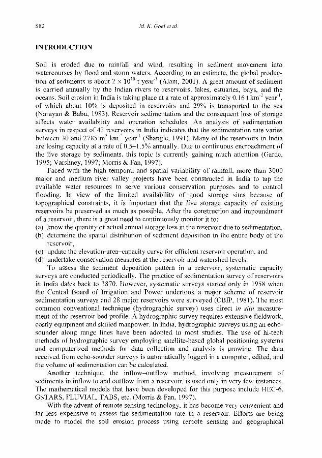
Bargi is a composite earth and masonry dam, 5374.39 m long, located near the village of Bargi in the Jabalpur district. The project was envisaged as a multipurpose scheme to serve the water needs for domestic and industrial purposes, irrigation and hydropower generation. The dam is located 43 km downstream of Jabalpur city at latitude 22°56'30"N and longitude 79°55'30"E. The index map of the basin is presented in Fig. 1. The catchment area at the dam site is 14 556 km". The Bargi Reservoir (now known as Rani Avanti Bai Sagar), has maximum, full and dead storage levels of 425.70, 422.76 and 403.55 m, respectively. The gross, live, and dead storage


- ORDINARY RAINGAUOE STATION • • . y

m SELF RECORDING RAINGAUOE »* STATION

V ^ DAM SITE

w - RIVER

* 6AUGE SITE M**! _ J É 1

Fig. 1 Index map of Narmada basin up to Bargi Dam.

capacities of the reservoir are 3.92, 3.18 and 0.740 x 109 nr, respectively. The maximum height of the masonry dam is 69.80 m while that of the earth dam is 29 m. The reservoir has been classified as hilly according to the Indian Standard Code no. 5477. The shape of the reservoir is almost elongated. Its longest periphery from the axis is about 80 km.

The average annual rainfall in the catchment up to Jamtara is 1414 mm. About 94% of the annual total rainfall occurs during the monsoon season (July-October). The average annual inflow at the dam site is 7197 x 106 m3. The dam was first impounded up to elevation 407.5 m a.m.s.l. in 1988. In 1989 and 1990, the reservoir was filled up to elevations 418.5 and 422.76 m a.m.s.l., respectively. No hydrographie survey has been carried out for the reservoir so far.

DATA AVAILABILITY

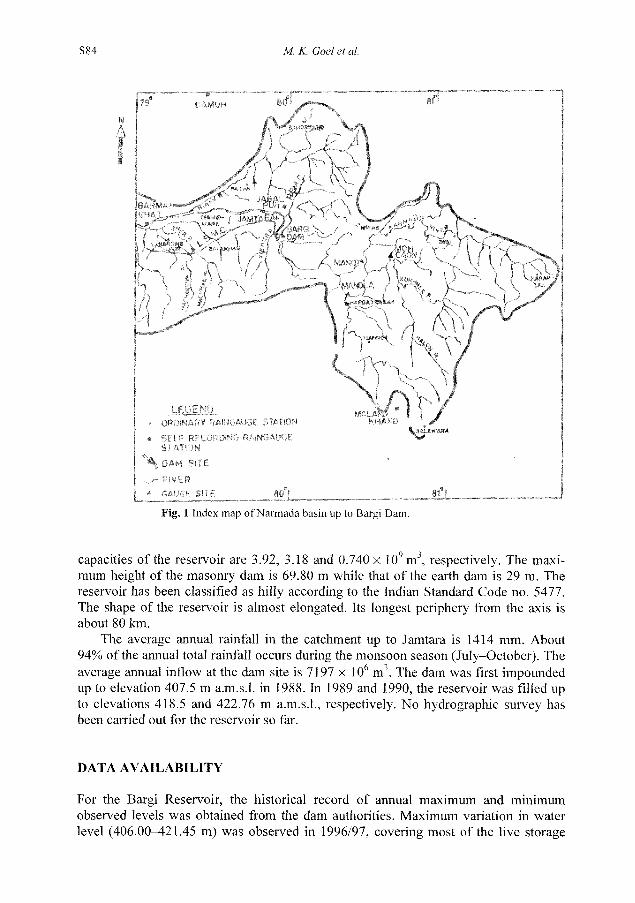
For the Bargi Reservoir, the historical record of annual maximum and minimum observed levels was obtained from the dam authorities. Maximum variation in water level (406.00-421.45 m) was observed in 1996/97, covering most of the live storage


zone (403.55—422.76 m). Therefore, the period from October 1996 to June 1997 was selected for analysis.

The multispectral data of IRS-1C satellite, LISS-III sensor were available for the period of analysis and were used in this study. The Bargi Reservoir water spread was covered in one scene of Path 100 and Row 56 of the satellite. Based on the status and availability of remote sensing data and the time spacing between the satellite data, nine scenes were obtained for the following dates of pass: 10 October 1996, 3 November 1996, 27 November 1996, 7 February 1997, 3 March 1997, 27 March 1997, 20 April 1997, 14 May 1997, and 7 July 1997. The water levels on these days were obtained from the dam authorities.

INTERPRETATION AND ANALYSIS

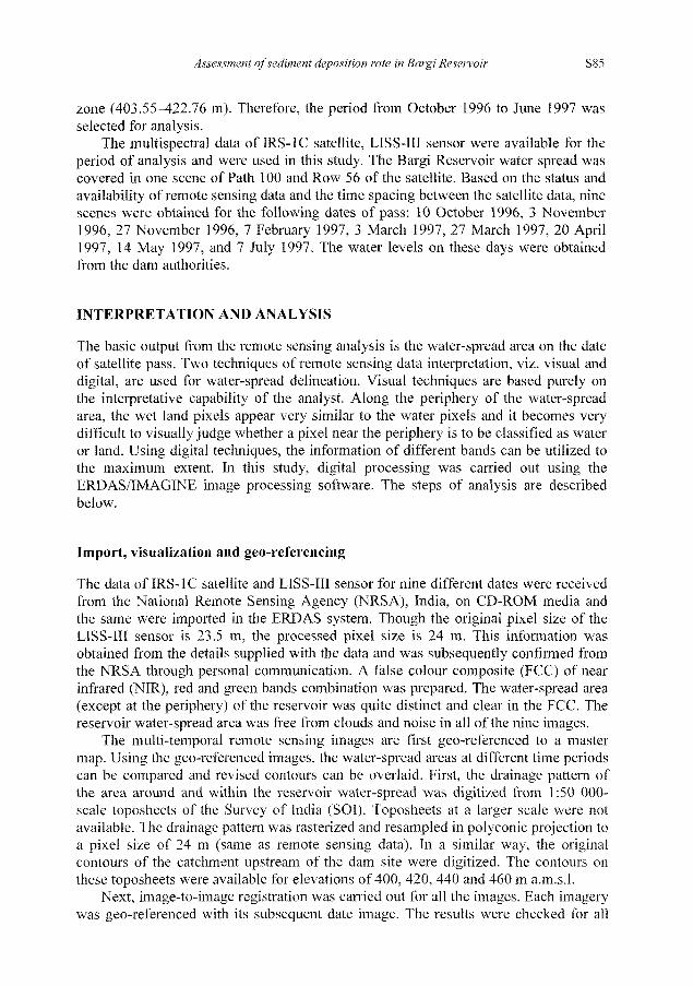
The basic output from the remote sensing analysis is the water-spread area on the date of satellite pass. Two techniques of remote sensing data interpretation, viz. visual and digital, are used for water-spread delineation. Visual techniques are based purely on the interpretative capability of the analyst. Along the periphery of the water-spread area, the wet land pixels appear very similar to the water pixels and it becomes very difficult to visually judge whether a pixel near the periphery is to be classified as water or land. Using digital techniques, the information of different bands can be utilized to the maximum extent. In this study, digital processing was carried out using the ERDAS/IMAGINE image processing software. The steps of analysis are described below.

Import, visualization and geo-referencing

The data of IRS-1C satellite and LISS-III sensor for nine different dates were received from the National Remote Sensing Agency (NRSA), India, on CD-ROM media and the same were imported in the ERDAS system. Though the original pixel size of the LISS-III sensor is 23.5 m, the processed pixel size is 24 m. This information was obtained from the details supplied with the data and was subsequently confirmed from the NRSA through personal communication. A false colour composite (FCC) of near infrared (NIR), red and green bands combination was prepared. The water-spread area (except at the periphery) of the reservoir was quite distinct and clear in the FCC. The reservoir water-spread area was free from clouds and noise in all of the nine images.

The multi-temporal remote sensing images are first geo-referenced to a master map. Using the geo-referenced images, the water-spread areas at different time periods can be compared and revised contours can be overlaid. First, the drainage pattern of the area around and within the reservoir water-spread was digitized from 1:50 000-scale toposheets of the Survey of India (SOI). Toposheets at a larger scale were not available. The drainage pattern was rasterized and resampled in polyconic projection to a pixel size of 24 m (same as remote sensing data). In a similar way, the original contours of the catchment upstream of the dam site were digitized. The contours on these toposheets were available for elevations of 400, 420, 440 and 460 m a.m.s.l.

Next, image-to-image registration was carried out for all the images. Each imagery was geo-referenced with its subsequent date image. The results were checked for all


80"tTE m°B% 80'16-E 8 0 ' 2 «

eO-O'E 8a*8-E 80»«-E 80°24'E

Fig. 2 Near-infrared image of Bargi Reservoir on 10 October 1996 overlaid with water-spread image (white) of 7 June 1997.

the images by displaying two images at a time one over the other and comparing the two using the SWIPE facility. The match between the images was satisfactory. After image-to-image registration, the resulting images were geo-referenced with the drainage map. The geo-referenced NIR-band image of the Bargi Reservoir of 10 October 1996 is shown in Fig. 2. The water-spread image of 7 June 1997 is overlaid on this image to present an overall view of the variation in the water-spread area.

IDENTIFICATION OF WATER PIXELS

In the visible region of the spectrum (0.4-0.7 urn), the transmittance of water is significant and the absorptance and reflectance are low. The absorptance of water rises rapidly in the NIR band, where both the reflectance and transmittance are low. At NIR wavelengths, water apparently acts as a black body absorber. Though the spectral signatures of water are quite distinct from other land uses such as vegetation, built-up areas and soil surfaces, the identification of water pixels at the water/soil interface is very difficult and depends on the interpretative ability of the analyst. Deep water bodies have quite distinct and clear representation as compared to shallow water. Shallow water can be mistaken for soil, while saturated soil can be mistaken for water, especially along the periphery of the reservoir. To differentiate water pixels from the adjacent wet land pixels, comparative analysis of the digital numbers in different bands was carried out. The methodologies commonly used in digital processing are classification, thresholding and modelling.


After analysing the spectral reflectance of water pixels in various imageries, an algorithm was used to identify water pixels using data of different bands. The algorithm matches the digital number (DN) value of a pixel with that of water and then identifies whether a pixel represents water or not. In addition, it also checks for the normalized difference water index, NDWI, which can be defined as:

ND WI = (Green - NIR)/(Green + NIR) ( 1 )

A separate NDWI image of the area is created. In all the images, it was found that the NDWI value for water is either equal to or greater than 0.44. The algorithm checks for the following condition for each pixel:

"If the digital number of NIR band of a pixel is less than the digital number of the red band and the green band, and the NDWI is >0.44, then it is classified as water, otherwise not"

In other words, if the condition is satisfied, then the pixel is recorded as water, otherwise not.

Since the absorptance of electromagnetic radiation by water is at a maximum in the NIR spectral region, the DN value of water pixels will be appreciably less than those of other land cover pixels. Even if the water depth is very shallow, the increased absorptance in the NIR band causes the DN value to be less than that of red and green bands. This algorithm differentiates water pixels from other pixels and was applied in the form of a model in the ERDAS/IMAGINE software; model runs were taken with images of different dates. The resulting images of water pixels were compared with the NIR images and the standard FCC. The results were found to be satisfactory in all the cases. The biggest advantage of this method was that it avoided the necessity of selecting different limits in different images as required in density slicing.

Removal of discontinuous pixels

Since the area within a contour is continuous, it is required that the isolated water pixels surrounding the water-spread area and/or located within the islands be removed from the interpreted water image. Similarly, the water pixels downstream of the dam do not form part of reservoir and need to be removed.

To remove most of these unwanted pixels, a mask was generated from the edited water image of 10 October 1996. The water image of this date was manually edited to remove the discontinuous pixels and the downstream river pixels. Next, the water images corresponding to remote sensing images of all dates were obtained by applying the model as mentioned above. The mask was superimposed and all the pixels outside the mask were treated as if they are not part of the reservoir. Most of the discontinuous pixels could be removed in this step. However, some of the pixels that were discontinuous and lie within the mask still needed to be edited. To remove these pixels, a GIS utility known as CLUMP was used. An 8-connected clump image was formed for all the water images. This utility created a clump around the discontinuous pixels and assigned different values to different clumps. Using the MODELER option, these clumped pixels were removed so that only continuous water-spread area remained in the water image.


Removal of extended tail and channels

The main river at the tail end of the reservoir and numerous small channels joining the reservoir from different directions around its periphery are also classified as water. However, the elevation of water in these channels and the main river remains slightly higher than the water surface of a reservoir receiving inflow through perennial streams. So, the extended tail and channels must be removed from the point of termination of spread. The selection of truncation point is subjective and may be based on the difference between the water levels in the subsequent date imageries.

In the present case, there were no extended channels around the periphery of the reservoir. Further, there was no need to identify the tail end in eight out of nine imageries except for the image of October 1996. In eight imageries, the termination of water-spread area was obvious.

Derivation of revised contours

After finalizing the water-spread area for a particular image, the periphery of the water-spread area was derived using various digital processing techniques. First, the islands within the spread area and the diagonally connected pixels were removed. This was achieved using the CLUMP module, in the same way as was done for removing the discontinuous water pixels. Then, three different kinds of filters, namely Edge Detection, Horizontal and Vertical were convoluted with the total water-spread image. After obtaining the final peripheral pixels, the elevation values were assigned to them

22°56'N

22°48'N

22o40'N

8OT

Elevation

a i l

• 1

4QA:Jb m

410.0S m

411.80 m

413.75 m

415.60m

419.55 m

420.95 in

421.45 m

•E 80-8-E

Scale

10 0

8D»ia'E

Kilometers

fi

80°24'E

£

80°0'E 8(F8"E

Fig. 3 Revised contours of Bargi Reservoir.


using the MODELER option. The revised contours of the reservoir water-spread area, as obtained from remote sensing analysis are presented in Fig. 3.

Calculation of revised capacity

After finalizing the water-spread areas of all the images, the histograms were analysed and the water pixels in each image were recorded. The water-spread area at any elevation was obtained by multiplying the number of water pixels by the size of one pixel (24 m x 24 m). The reservoir capacity between two consecutive reservoir elevations was computed using the prismoidal formula:

V = AH(AI+A2+-JA~^)/3 (2)

where V is the volume between two consecutive elevations 1 and 2, and A \ and A2 are the contour areas and AH is the difference between elevations 1 and 2. The original elevation-capacity table before the impoundment of the dam (1988) was obtained from the Reservoir Operation & Maintenance Manual of the Narmada Valley Development Authority (NVDA, 1992), Government of Madhya Pradesh. From the original elevation-capacity table, the original capacity at the intermediate elevations (reservoir elevations on the dates of satellite pass) was obtained by linear interpolation. The revised volume was compared with the original volume in each zone and the difference between the two gave the capacity loss due to sedimentation.

The cumulative revised capacity of the reservoir at the lowest observed level (406.00 m) was assumed to be the same as the original cumulative capacity (1010.00 x 106 m3) at this elevation. Above this level, the cumulative capacities between the consecutive levels were added together to arrive at the cumulative revised capacity at the maximum observed level (421.45 m). The calculation is presented in Table 1.

DISCUSSION OF RESULTS

The results show that the revised capacity in the zone under consideration (between elevation 406.00 and 421.45 m a.m.s. 1.) is 2558.89 x 106m3, while the original

Table 1 Calculation of sediment deposition in Bargi Reservoir using remote sensing.

Date of satellite pass

10 October 1996 3 March 1996 27 November 1996 7 February 1997 3 March 1997 27 March 1997 20 April 1997 14Mav 1997 7 June 1997

Reservoir elevation above m.s.l. (m)

421.45 420.95 419.55 415.60 413.75 411.80 410.05 407.35 406.00

Revised area (x l()6nr)

256.19 250.43 237.68 187.53 164.84 140.40 119.58 093.11 079.11

Original volume (x 106m3)

139.97 391.90 860.07 306.91 262.16 213.94 290.03 120.85

1010.00

Revised volume (x 10W)

126.65 341.64 837.84 325.72 297.29 227.24 286.39 116.12

1010.00

Original cumulative volume (x 106m3)

3595.83 3455.87 3063.96 2203.89 1896.98 1634.82 1420.88 1130.85 1010.00

Revised cumulative volume (x 106 m3)

3568.89 3442.24 3100.60 2262.76 1937.04 1639.75 1412.51 1126.12 1010.00

Note: Revised values were calculated from remote sensing data.


capacity as calculated and envisaged in the project before the impoundment of the dam was 2585.56 x 106 mJ. Thus, it can be inferred that 26.67 x 106 nr' of the capacity has been lost to sedimentation in the zone under study in a period of eight years (1989— 1996). The year 1988 was not considered because the impoundment of the dam in that year was only up to 407 m. Thus, the rate of sedimentation in the reservoir is calculated as 3.33 x 106 mJ year"1. In India, the sedimentation rate is generally specified as loss per unit catchment area per year; therefore, the loss rate in the zone under study is 229.03 m3 km"2 year"1.

The results of this study were compared with the sedimentation study report prepared by Central Water Commission (CWC, 1990), in which a trap efficiency of 95% was assumed. Based on the upstream developments, the report predicted that the total sediment trapped in the reservoir would be 57.465 x 106m3 during the period 1989-1993 and 56.550 x 106 m3 during the period 1994-1999. The total sediment predicted to get trapped in the reservoir (367^122.76 m a.m.s.l.) during the period from 1989 to 1996 was 85.74 x l0 6 m 3 . The results of the present study show that 26.67 x l 0 6 m 3 of sediment was deposited in the zone between 406.00 and 421.45 m a.m.s.l. The height of the dead storage zone of this reservoir (367.00-403.55 m) is about 36.5 m while that of the live storage zone (403.55^422.76 m) is 19.21 m. The tail portion of the Bargi Reservoir is quite significant compared to the main body of the reservoir. Since the reduction in velocity in the tail portion of this reservoir is only marginal, the suspended sediment carrying capacity does not reduce appreciably, resulting in the transportation of most of the sediments towards the main reservoir and their deposition at greater depths.

80-0'E 8<F8'E 80°16'E

80*D'E 80-8-E 80°1S'E

Fig. 4 Comparison of original contour of elevation 420.00 m (black) with derived contour of elevation 419.55 m (grey).

Assessment of sediment deposition rate in Bargi Reservoir S 91

It is important to note that the accuracy of assessment of sedimentation depends on the accuracy of the original capacity table. The Bargi Reservoir has a dendritic shape with a number of narrow but long branches jutting out at many places, in addition to the main tail. A comparison between the original and revised contours was also made. The original contour of 420 m and the revised contour of 419.55 m elevation are plotted in Fig. 4. At a few locations, it is observed that the original contour is lying inside of the revised contour, which should not happen in normal circumstances unless significant erosion has occurred at those locations. The comparison further shows that, at other locations, the contour derived from remote sensing corresponds quite closely with the original contour.

CONCLUDING REMARKS

The present study of Bargi Reservoir demonstrates that the remote sensing technique is a time- and cost-effective and convenient approach to estimate the elevation-area-capacity curves for a reservoir. The procedure to remove the discontinuous pixels and the derivation of contours has been considerably automated.

The conventional methods, such as hydrographie surveys, are laborious, costly and time-consuming. For these reasons, the hydrographie surveys of reservoirs are normally conducted at a frequency of 5-15 years, though the recommended frequency is every five years. Remote sensing techniques can be used as a cost- and time-effective tool to estimate capacity loss.

The major limitation of the remote sensing-based approach is that the revised capacity below the lowest observed and above the highest observed reservoir water levels cannot be determined. It is only possible to calculate the sedimentation rate within the zone of fluctuation of reservoir water level. From the point of view of operation of the reservoir, this limitation is not very significant. Since the reservoir level rarely falls below the minimum drawdown level in normal years, the interest mainly lies in knowing the revised capacity and the sediment deposition pattern within the live storage zone. However, if the sedimentation in the entire reservoir is to be found, in addition to remote sensing data analysis, the hydrographie survey within the water-spread area corresponding to the lowest observed elevation may be carried out. This will decrease the amount of effort required carry out the hydrographie survey.

Further, it may be seen that the estimation of sedimentation by remote sensing is highly sensitive to the accuracy of: (a) the determined water-spread area, (b) water level information, and (c) the original elevation-area-capacity table. However, if the water level information is exact and the water-spread area is interpreted accurately, it is possible to find the revised elevation-area-capacity curves quite precisely.

Accuracy in the identification of water pixels, particularly at the tail end of a reservoir, affect the accuracy of sedimentation assessment using remote sensing. Further, the satellites of higher spatial resolution are now becoming available and the data of these must be utilized to increase the accuracy of the water-spread area determination. Remote sensing images can be chosen at closer time intervals so that the revised water-spread area may be obtained at smaller elevation intervals, thereby increasing the accuracy of sedimentation assessment.


REFERENCES

Alam, S. (2001) A critical evaluation of sedimentation management design practice. Hydropower & Dams 1, 54-59. Baban, S. M. & Yusuf, K. W. (2001) Modelling soil erosion in tropical environments using remote sensing and

geographical information systems. Hydro!. Sci. J. 46(2), 191.198. CB1P (Central Board of Irrigation and Power) (1981) Sedimentation studies in reservoirs. Tech. Report no. 20, vol. 2,

CBIP, New Delhi, India. CWC (Central Water Commission ) (1990) Sedimentation study of Bargi Project (MP.). Central Water Commission, New

Delhi, India. Garde, R. J. (1995) Reservoir sedimentation. State of art report of Indian National Committee on Hydrology.

INCOH/SAR-6/95. National Institute of Hydrology, Roorkee, India. Goel, M. K. & Jain, Sanjav K. (1996) Evaluation of reservoir sedimentation usine multi-temporal IRS-1A I.1SS-11 data.

Asian Pacific Remote Sens. & GIS.I. 8(2), 39^*3. Goel, M. K. & Jain, Sharad K. (1998) Reservoir sedimentation study for Ukai Dam using satellite data. Report no. UM-

1 /97-98, National Institute of I lydrology, Roorkee, India. Gupta, S. C. (1999) Status paper on reservoir sedimentation assessment using remote sensing techniques. In: Proc.

National Workshop on Reservoir Sedimentation Assessment Using Remote Sensing Data. National Institute of Hydrology, Roorkee, India.

Jain, M K. & Kothvari, U. C. (2000) Estimation of soil erosion and sediment vield using GIS. Hydro!. Sci. ./. 45(5), 771 — 786.

Jain, S. K. & Goel, M. K. (2002) Assessing the vulnerability to soil erosion of the Ukai Dam catchment usins» remote sensing and G1S. Hydro!. Sci. J. 47( 1 ), 31 -40.

Jain, S. K., Singh, P. & Seth, S. M. (2002) Assessment of sedimentation in Bhakra Reservoir in the western Himalayan region using remotely sensed data. Hydro! Sci. J. 47(2), 203-212.

Manvalan, P., Rajegowda, G. E. & Srinivas, M. V. (1991) Capacity evaluation of Ghatprabha Reservoir using digital analysis of 1RS L1SS-II data. Project report no. B/003/91, Regional Remote Sensing Service Centre, Bangalore, India.

Morris, G. E. & Fan, J. (1997) Reservoir Sedimentation Handbook Design and Management of Dams, Reservoirs, and Watersheds for Sustainable Use. Tata McGraw-Hill, New York, USA.

Narayan, D. V. V. & Babu, R. (1983) Estimation of soil erosion in India../, brig. Drain. Engng 109(4), 419—43). NVDA (Narmada Valley Development Authority) (1992) Reservoir Operation & Maintenance Manual. Rani Avanti Bai

Sagar Project, Jabalpur, Madhya Pradesh, India. Shangle, A. K. (1991) Reservoir sedimentation status in India, jalvigyan Sameeksha. 6(1&2). Indian National Committee

on Hydrology, National Institute of Hydrology, Roorkee, India. Varshney, R. S. ( 1997) Impact of siltation on the useful life of large reservoirs. State of art report no. INCOH/SAR-11 /97,

INCOH, National Institute of Hydrology, Roorkee, India.

Documents

Assessment of sediment deposition rate in Bargi Reservoir using