Wayne State University

Honors College Theses Irvin D. Reid Honors College

Winter 5-3-2015

No-Arbitrage Option Pricing and the BinomialAsset Pricing ModelNicholas S. HurleyWayne State University, NickHurley2011@yahoo.com

Follow this and additional works at: https://digitalcommons.wayne.edu/honorstheses

Part of the Probability Commons

This Honors Thesis is brought to you for free and open access by the Irvin D. Reid Honors College at DigitalCommons@WayneState. It has beenaccepted for inclusion in Honors College Theses by an authorized administrator of DigitalCommons@WayneState.

Recommended CitationHurley, Nicholas S., "No-Arbitrage Option Pricing and the Binomial Asset Pricing Model" (2015). Honors College Theses. 19.https://digitalcommons.wayne.edu/honorstheses/19

No-Arbitrage Option Pricing and the

Binomial Asset Pricing Model

Nicholas Hurley

May 3, 2015

1 Introduction

Financial markets often employ the use of securities, which are dened tobe any kind of tradable nancial asset. Common types of securities includestocks and bonds. A particular type of security, known as a derivative security(or simply, a derivative), are nancial instruments whose value is derived fromanother underlying security or asset (such as a stock). A common kind ofderivative is an option, which is a contract that gives the holder the rightbut not the obligation to go through with the terms of said contract. Anexample of an option is the European Option, which we will use commonlythroughout the following sections:

DEFINITION 1.1 (European Option). A European call(put) option givesthe holder the right, but not the obligation, to buy(sell) an asset at a speciedtime, t, for a specied price, K.The payout of the option is then max(St−K, 0) (or for a put option, max(K−St, 0)).

Because options can be traded - bought and sold, a problem arises on howto value the option (at a particular time, namely when the option is rstcreated). The concept of evaluating an option, typically before the futurevalues of the underlying security are known, is referred to as option pricing.The binomial asset pricing model allows us to evaluate options by usinga "discrete-time" model of the behavior of the underlying security. Whilethe binomial model is rather simplistic, it does provide a powerful tool inunderstanding the fundamental aspects of option pricing and no-arbitragepricing theory.Before going into any greater detail on the binomial model, there are severalimportant nancial terms that will be used:

• Stock Market: The stock market is where stocks are traded. Stocksare a type of security that represents partial ownership of a company.Since stocks tend to uctuate in value they are generally considered arisky asset. A unit of stock is known as a share.

1

• Short and Long Positions: An investor dealing with a security suchas stocks will be in the long position if he owns shares and will be inthe short position if he owes shares. If an investor owns X amount ofshares he is said to be long X shares, similarly if he sells X amountof shares ("borrows" them and sells them) he is said to be short Xshares. If the investor is in the short position he must eventually buythe stock to repay the broker (individual/rm that organizes buy/sellorders from investors) he bought the shares through. If the stock hasdecreased in value then the investor will have made a prot (and if itincreases, a loss). The concept of the short and long position is notexclusive to stocks, it can also be used with any security, commodity,or option that makes sense. In the case of options, the person who sellsthe option is in the short position, with the buyer in the long position.

• Money Market: The money market includes securities that are prac-tically risk-less. While the potential long-term payos of putting moneyin the money market are small in comparison to that of investing in thestock market, money in the money market accrues interest over time.

• Interest Rate: The interest rate, represented by the letter r ≥ 0, willbe dened such that for every dollar put into the money market theinvestor will receive (1 + r)t at time t.

• Portfolio: A portfolio is simply a collection of securities. A tool thatwe will use with the binomial model in the proceeding sections is that ofa replicating portfolio. Creating a replicating portfolio involves invest-ing in both the stock and money markets such that the wealth of theportfolio is equal to the value of the payo of the option regardless ofthe behavior of the stock (underlying asset of the option) at each timeperiod. A key component of no-arbitrage option pricing is creating areplicating portfolio.

• Arbitrage: A trading strategy that exhibits arbitrage is one that startswith no money, has zero probability of losing money, and positive prob-ability of making money. If arbitrage is possible, then wealth can begenerated from nothing. Real markets will occasionally exhibit arbi-trage but trading will quickly remove it. The proceeding examples takea look at simple cases of arbitrage and how an asset can be priced toavoid it.

EXAMPLE 1.1. Consider two markets, Market A and Market B, where inMarket A a crate of apples is valued at $20 a crate and in Market B they are

2

valued at $22 a crate. Taking advantage of a dierence in price, an investorlooking at these two markets could quickly buy in Market A and sell in MarketB - making a guaranteed risk-free prot. Such an event provides an arbitrageopportunity only for quick investors, as trading will quickly eliminate the pricedierence. Something to note is that it is possible for there to be transactioncosts (suppose it costs $5 per crate to get a crate of apples from Market A toMarket B), essentially eliminating any arbitrage opportunity.

EXAMPLE 1.2 (Hedging and arbitrage). In the previous example we dealtwith a simple dierence in market prices, in the following example we discusswhat is known as a hedging transaction. A hedging transaction is when aninvestor has a primary security/portfolio position and establishes a secondaryposition to counterbalance some or all of the risk of the primary position.A simple hedging example is as follows:Suppose an investor owns a stock originally valued at $50 that then increasesto $60. If the investor is worried about a future fall in price he can simplysell the stock, but what if he can't or doesn't want to? They could protect theprot by selling short the stock for $60, leaving the investor with an overallgain of $10 while maintaining their established long stock position. Whetherthe stock rises or falls the two positions oset and the investor is locked inat a $10 prot. While the investor's previously gained prot is essentiallyguaranteed there is no chance of increasing it, given the new position.Now, consider two hedging examples that exhibit an arbitrage opportunity:

1. Suppose we have a portfolio consisting of a packaged bundle of twostocks - Stock A valued at $5 and Stock B valued at $6. An investorwould be able to gain a risk-free prot if there is an imbalance in price ofthe portfolio and the value of a single share of both stocks. If the priceof the portfolio is overvalued at $12 an investor could sell short theportfolio and buy the stocks individually - gaining an initial cash owof $12− $(6 + 5) = $1. On the other hand, if the price of the portfoliois undervalued at $10 an investor could sell short the two stocks andbuy the portfolio - gaining an initial cash ow of $(6 + 5)− $10 = $1.Note that the hedge is self-nancing and the net future cash ow iszero as the investor owns the stocks to cover the short position. Theabove instances exhibit an arbitrage opportunity, and like the previoustwo examples, investors will take advantage causing the stock prices togo up and the price of the portfolio to go down (and vice versa for thesecond case) until an arbitrage free price for the portfolio is reached(the price of the portfolio equals the price of the two stocks).

2. Suppose now that we have two assets and one period (time zero and

3

time one). Asset A has a current price of $1000 and, in the nextperiod, a future cash ow of $1100, and Asset B has a current price of$2000 and, in the next period, a future cash ow of $2250. Forming aportfolio by buying and selling these two assets separately has an initialcash ow of $0 - the portfolio created is costless. If an investor wantedto construct a portfolio to take advantage of an arbitrage opportunitythey could short sell two units of Asset A and buy one unit of Asset B.The initial cash ow is −2($1000) + 1($2000) = $0, and at the end ofthe period we have an expected cash ow of −2($1100)+1($2250) = $50.This constitutes an arbitrage opportunity since it is costless to constructthe portfolio but still produces a positive future cash ow - the investormakes a risk-less prot. Similar to the previous examples, investorswould take advantage of such an opportunity as much as they can untilthe opportunity eventually disappears.

EXAMPLE 1.3 (No-arbitrage price of a forward contract). A forward con-tract, or simply a forward, is a derivative security in which two parties agreeto buy or sell an asset at a specied time in the future at a specied price,F , today. There is no cost in entering a forward contract, the price F isn'tpayed until the specied time period (when the asset is bought/sold). If attime 0 the forward contract is created and at time t the asset is traded, thenthe no-arbitrage price of the forward is:

F = S0(1 + r)t.

Where S0 is the time 0 price of the asset, and r is the interest rate. Thepayo of the contract, at time t, is St−F for the buyer of the contract (longposition) and F −St for the seller (short position). If the price of the forwardis not S0(1 + r)t, then there is an arbitrage:

• If F > S0(1 + r)t: At time 0, an investor can borrow $S0 and buy theasset. They can then take the short position on the forward contract.At time t, the asset is sold for the agreed upon price F and the loanfrom time 0 is paid o. The investor is left with a risk-free prot ofF − S0(1 + r)t.

• If F < S0(1 + r)t: At time 0, an investor can short sell one unit of theasset and lend $S0. They can then take the long position on the forwardcontract. At time t, the asset is bought for the agreed upon price F ,the short sold asset is returned, and the loan is recovered (which hassince grown to S0(1 + r)t). The investor is left with a risk-free prot ofS0(1 + r)t − F .

4

2 The Binomial Model

The binomial asset-pricing model provides a simple model for understandingthe no-arbitrage pricing of options. We start with the simple one-periodmodel and then generalize to a more realistic multi-period model.

2.1 The One-Period Binomial Model

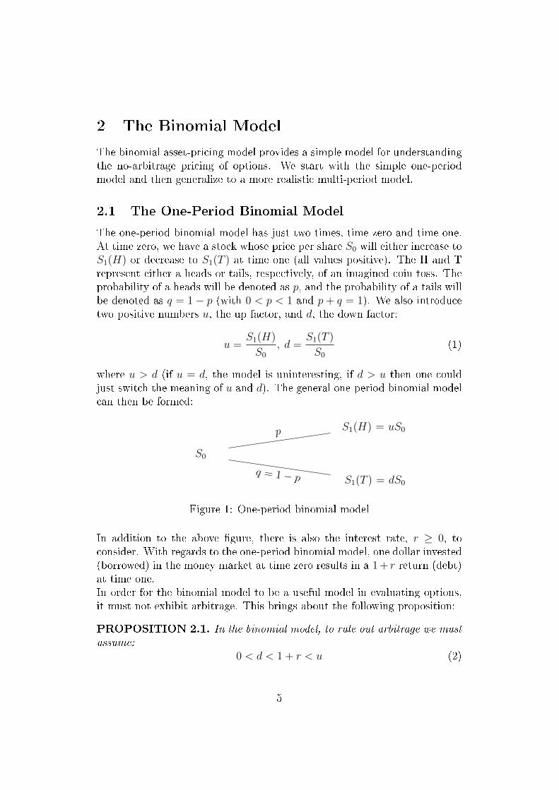
The one-period binomial model has just two times, time zero and time one.At time zero, we have a stock whose price per share S0 will either increase toS1(H) or decrease to S1(T ) at time one (all values positive). The H and Trepresent either a heads or tails, respectively, of an imagined coin toss. Theprobability of a heads will be denoted as p, and the probability of a tails willbe denoted as q = 1− p (with 0 < p < 1 and p + q = 1). We also introducetwo positive numbers u, the up factor, and d, the down factor:

u =S1(H)

S0

, d =S1(T )

S0

(1)

where u > d (if u = d, the model is uninteresting, if d > u then one couldjust switch the meaning of u and d). The general one-period binomial modelcan then be formed:

S0

S1(H) = uS0

S1(T ) = dS0

p

q = 1− p

Figure 1: One-period binomial model

In addition to the above gure, there is also the interest rate, r ≥ 0, toconsider. With regards to the one-period binomial model, one dollar invested(borrowed) in the money market at time zero results in a 1 + r return (debt)at time one.In order for the binomial model to be a useful model in evaluating options,it must not exhibit arbitrage. This brings about the following proposition:

PROPOSITION 2.1. In the binomial model, to rule out arbitrage we mustassume:

0 < d < 1 + r < u (2)

5

Proof. The rst inequality, 0 < d, is assumed from the positivity of stockprices. Looking at a one-period binomial model:

• If d ≥ 1 + r: An investor could, at time zero, borrow $S0 from themoney market and buy one share of stock. The investor's stock is thenworth either uS0 or dS0 at time one, depending on the coin toss (heads,tails respectively). Even in the worst case scenario, a tails, the investorhas at least a stock worth enough to pay back the money market debt($(1 + r)S0 at time one) with a positive probability, p > 0, of makingprot since u > d ≥ 1 + r.

• If u ≤ 1 + r: An investor could, at time zero, short sell the stock andinvest $S0 in the money market. The short sold stock is then wortheither uS0 or dS0 at time one, depending on the coin toss (heads, tailsrespectively). Even in the worst case scenario, a heads, the investor hasat least enough return on the money market loan ($(1 + r)S0 at timeone) to replace the stock with a positive probability, q = 1− p > 0, ofmaking prot since d < u ≤ 1 + r.

Before going through the process of pricing a European call option using thebinomial model, there are several principal assumptions we must consider:

• shares of stock can be subdivided for sale or purchase,

• the interest rate for investing is the same as the interest rate for bor-rowing,

• the purchase price of stock is the same as the selling price,

• the stock can take only two possible values in the next period.

In the general one-period binomial model, we dene a derivative security tobe a security whose payo is V1(H) or V1(T ) depending on the coin toss. Fora European call option, the payo is V1 = max(S1 − K, 0) where S1 is thevalue of the stock at time one and K is the strike price. To determine V0,the price of the derivative security at time zero, we construct a replicatingportfolio. Suppose we begin with a portfolio that has starting wealth X0 andwe buy ∆0 shares of stock, our cash position at time zero is then X0−∆0S0.The value of our portfolio (contains stock and money market account) attime one is:

X1 = ∆0S1 + (1 + r)(X0 −∆0S0) = (1 + r)X0 + ∆0(S1 − (1 + r)S0). (3)

6

In order to properly replicate the portfolio we must choose X0 and ∆0 suchthat X1(H) = V1(H) and X1(T ) = V1(T ). Note that at time zero we knowthe values of V1(H) and V1(T ), we just don't know which one will be realized.Using this requirement and equation (3) we get the following equations:

X0 + ∆0(1

1 + rS1(H)− S0) =

1

1 + rV1(H), (4)

X0 + ∆0(1

1 + rS1(T )− S0) =

1

1 + rV1(T ). (5)

In order to solve for our two unknowns, X0 and ∆0, we multiply equation (4)by p and equation (5) by q (where q = 1− p) and then adding them togethergiving us:

X0 + ∆0(1

1 + r[pS1(H) + qS1(T )]− S0) =

1

1 + r[pV1(H) + qV1(T )]. (6)

If we choose p (and thus q) so that:

S0 =1

1 + r[pS1(H) + qS1(T )], (7)

the terms cancel and we are left with the equation

X0 =1

1 + r[pV1(H) + qV1(T )]. (8)

By putting (7) in the following form (doing a little substitution),

S0 =1

1 + r[puS0 + (1− p)dS0] =

S0

1 + r[(u− d)p+ d],

we can solve for p and q:

p =(1 + r)− du− d

, q =u− (1 + r)

u− d. (9)

To nd ∆0 we can subtract (5) from (4) to get the delta-hedging formula:

∆0 =V1(H)− V1(T )

S1(H)− S1(T ). (10)

So, if an investor begins with wealth X0, given by (8), and buys ∆0 shares ofstock, given by (10), then at time one, they will have a portfolio worth eitherV1(H) or V1(T ) depending on the coin toss. We have properly constructed a

7

replicating portfolio and the derivative security at time zero should be pricedat

V0 =1

1 + r[pV1(H) + qV1(T )], (11)

which is the initial value X0 (of the replicating portfolio). Any other timezero price would introduce an arbitrage.The numbers p and q that we arbitrary selected and solved for (equation(9)) are both positive (no arbitrage assumption, equation (2))and sum toone. Because of this, we can think of p as the probability of heads and q asthe probability of tails. They are not the actual probabilities, p and q, butinstead what we call the risk-neutral probabilities. With the real probabilities,the average rate of growth of stock is greater than the rate of growth of aninvestment in the money market. If this wasn't the case then no one wouldbother investing in the risky stock market (compared to the money marketwhich has no risk). Therefore, p and q satisfy:

S0 <1

1 + r[pS1(H) + qS1(T )], (12)

unlike p and q that satisfy (7). Therefore, the risk-neutral probabilities as-sume that investors are neutral about risk - they typically are not, which iswhy p and q are not the actual probabilities. The risk-neutral probabilitiesare chosen so that the mean rate of return of any portfolio (comprised ofstock and money market accounts) equals the rate of growth of the moneymarket investment. If we consider pV1(H) + qV1(T ) to be the mean portfo-lio value under the risk-neutral probabilities (at time one), then rearranging(11) gives us the following relationship

r =[pV1(H) + qV1(T )]− V0

V0

, (13)

where r (the interest rate) is the rate of return from the money market.Because of this, the equation (11) is called the risk-neutral pricing formulafor the one-period binomial model. Risk-neutral pricing is described furtherin section 5.We illustrate the above replicating portfolio process with a simple example.

EXAMPLE 2.1 (Pricing a European call option). Consider a Europeancall option that goes through one time period - at time zero the option ispurchased and at time one the option is either exercised or it is not. Thepayo of the option is then max(S1 − K, 0), where K, the strike price, isthe agreed upon price paid for the stock. For the following example we haveS0 = 2, u = 2, d = 1/2, r = 1/4, and K = 2.5. From this we can easily

8

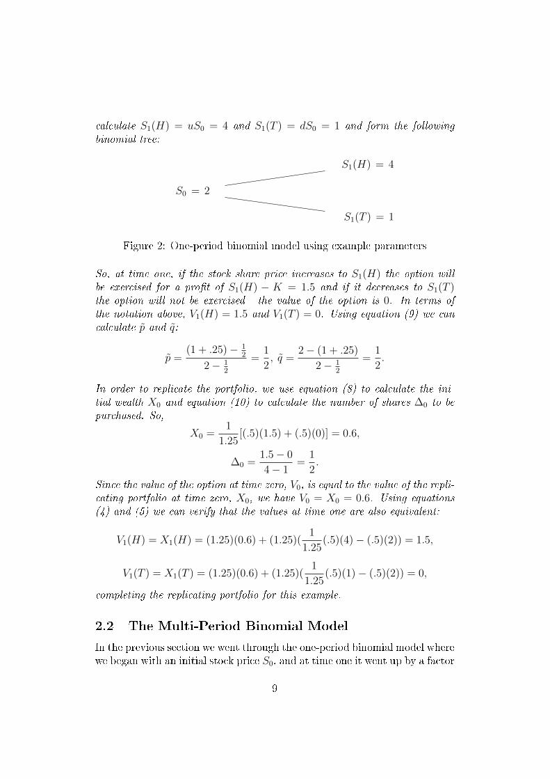
calculate S1(H) = uS0 = 4 and S1(T ) = dS0 = 1 and form the followingbinomial tree:

S0 = 2

S1(H) = 4

S1(T ) = 1

Figure 2: One-period binomial model using example parameters

So, at time one, if the stock share price increases to S1(H) the option willbe exercised for a prot of S1(H) − K = 1.5 and if it decreases to S1(T )the option will not be exercised - the value of the option is 0. In terms ofthe notation above, V1(H) = 1.5 and V1(T ) = 0. Using equation (9) we cancalculate p and q:

p =(1 + .25)− 1

2

2− 12

=1

2, q =

2− (1 + .25)

2− 12

=1

2.

In order to replicate the portfolio, we use equation (8) to calculate the ini-tial wealth X0 and equation (10) to calculate the number of shares ∆0 to bepurchased. So,

X0 =1

1.25[(.5)(1.5) + (.5)(0)] = 0.6,

∆0 =1.5− 0

4− 1=

1

2.

Since the value of the option at time zero, V0, is equal to the value of the repli-cating portfolio at time zero, X0, we have V0 = X0 = 0.6. Using equations(4) and (5) we can verify that the values at time one are also equivalent:

V1(H) = X1(H) = (1.25)(0.6) + (1.25)(1

1.25(.5)(4)− (.5)(2)) = 1.5,

V1(T ) = X1(T ) = (1.25)(0.6) + (1.25)(1

1.25(.5)(1)− (.5)(2)) = 0,

completing the replicating portfolio for this example.

2.2 The Multi-Period Binomial Model

In the previous section we went through the one-period binomial model wherewe began with an initial stock price S0, and at time one it went up by a factor

9

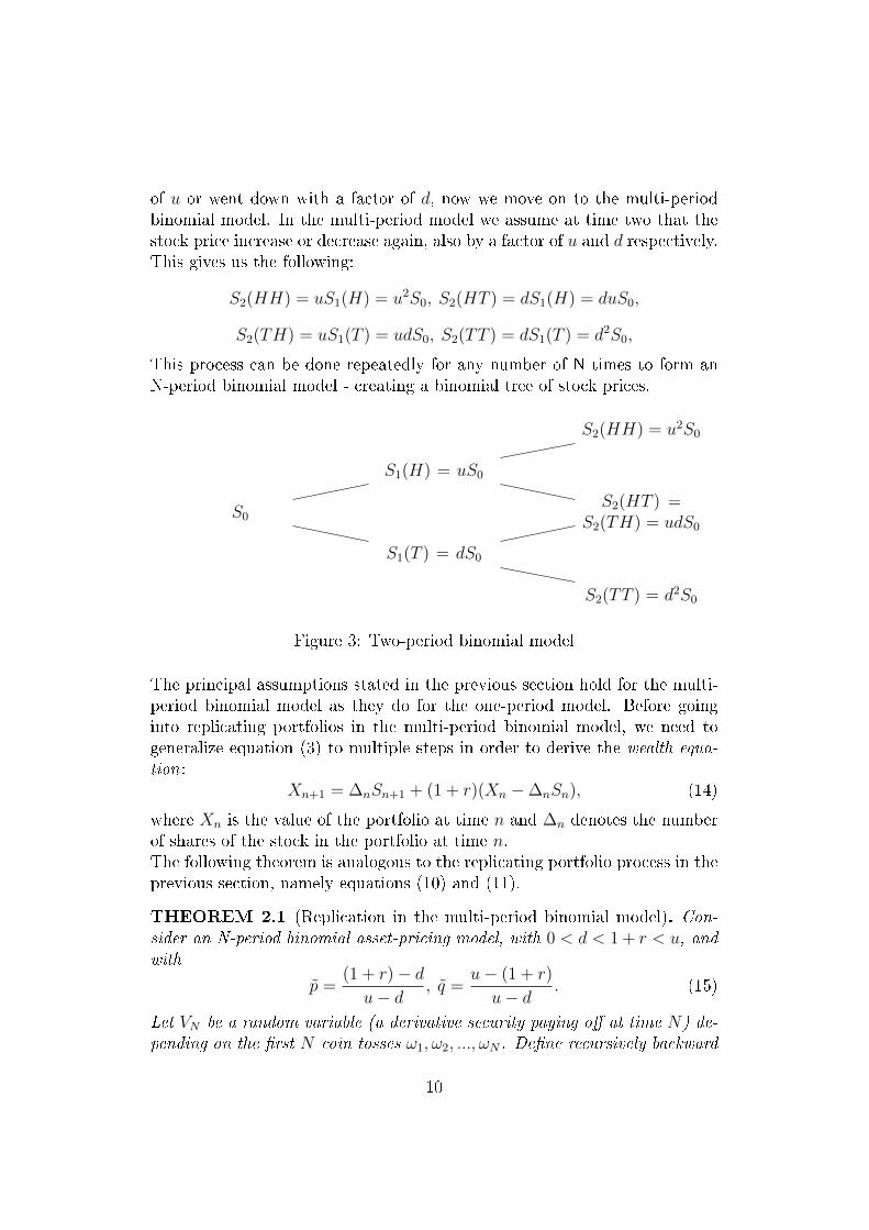
of u or went down with a factor of d, now we move on to the multi-periodbinomial model. In the multi-period model we assume at time two that thestock price increase or decrease again, also by a factor of u and d respectively.This gives us the following:

S2(HH) = uS1(H) = u2S0, S2(HT ) = dS1(H) = duS0,

S2(TH) = uS1(T ) = udS0, S2(TT ) = dS1(T ) = d2S0,

This process can be done repeatedly for any number of N times to form anN-period binomial model - creating a binomial tree of stock prices.

S0

S1(H) = uS0

S1(T ) = dS0

S2(HH) = u2S0

S2(HT ) =S2(TH) = udS0

S2(TT ) = d2S0

Figure 3: Two-period binomial model

The principal assumptions stated in the previous section hold for the multi-period binomial model as they do for the one-period model. Before goinginto replicating portfolios in the multi-period binomial model, we need togeneralize equation (3) to multiple steps in order to derive the wealth equa-tion:

Xn+1 = ∆nSn+1 + (1 + r)(Xn −∆nSn), (14)

where Xn is the value of the portfolio at time n and ∆n denotes the numberof shares of the stock in the portfolio at time n.The following theorem is analogous to the replicating portfolio process in theprevious section, namely equations (10) and (11).

THEOREM 2.1 (Replication in the multi-period binomial model). Con-sider an N-period binomial asset-pricing model, with 0 < d < 1 + r < u, andwith

p =(1 + r)− du− d

, q =u− (1 + r)

u− d. (15)

Let VN be a random variable (a derivative security paying o at time N) de-pending on the rst N coin tosses ω1, ω2, ..., ωN . Dene recursively backward

10

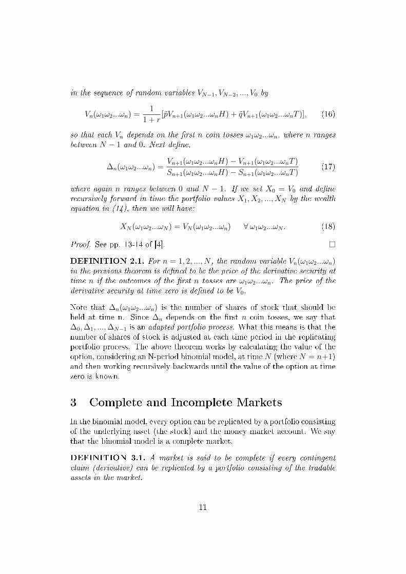
in the sequence of random variables VN−1, VN−2, ..., V0 by

Vn(ω1ω2...ωn) =1

1 + r[pVn+1(ω1ω2...ωnH) + qVn+1(ω1ω2...ωnT )], (16)

so that each Vn depends on the rst n coin tosses ω1ω2...ωn, where n rangesbetween N − 1 and 0. Next dene,

∆n(ω1ω2...ωn) =Vn+1(ω1ω2...ωnH)− Vn+1(ω1ω2...ωnT )

Sn+1(ω1ω2...ωnH)− Sn+1(ω1ω2...ωnT )(17)

where again n ranges between 0 and N − 1. If we set X0 = V0 and denerecursively forward in time the portfolio values X1, X2, ..., XN by the wealthequation in (14), then we will have:

XN(ω1ω2...ωN) = VN(ω1ω2...ωn) ∀ ω1ω2...ωN . (18)

Proof. See pp. 13-14 of [4].

DEFINITION 2.1. For n = 1, 2, ..., N , the random variable Vn(ω1ω2...ωn)in the previous theorem is dened to be the price of the derivative security attime n if the outcomes of the rst n tosses are ω1ω2...ωn. The price of thederivative security at time zero is dened to be V0.

Note that ∆n(ω1ω2...ωn) is the number of shares of stock that should beheld at time n. Since ∆n depends on the rst n coin tosses, we say that∆0,∆1, ...,∆N−1 is an adapted portfolio process. What this means is that thenumber of shares of stock is adjusted at each time period in the replicatingportfolio process. The above theorem works by calculating the value of theoption, considering an N-period binomial model, at timeN (whereN = n+1)and then working recursively backwards until the value of the option at timezero is known.

3 Complete and Incomplete Markets

In the binomial model, every option can be replicated by a portfolio consistingof the underlying asset (the stock) and the money market account. We saythat the binomial model is a complete market.

DEFINITION 3.1. A market is said to be complete if every contingentclaim (derivative) can be replicated by a portfolio consisting of the tradableassets in the market.

11

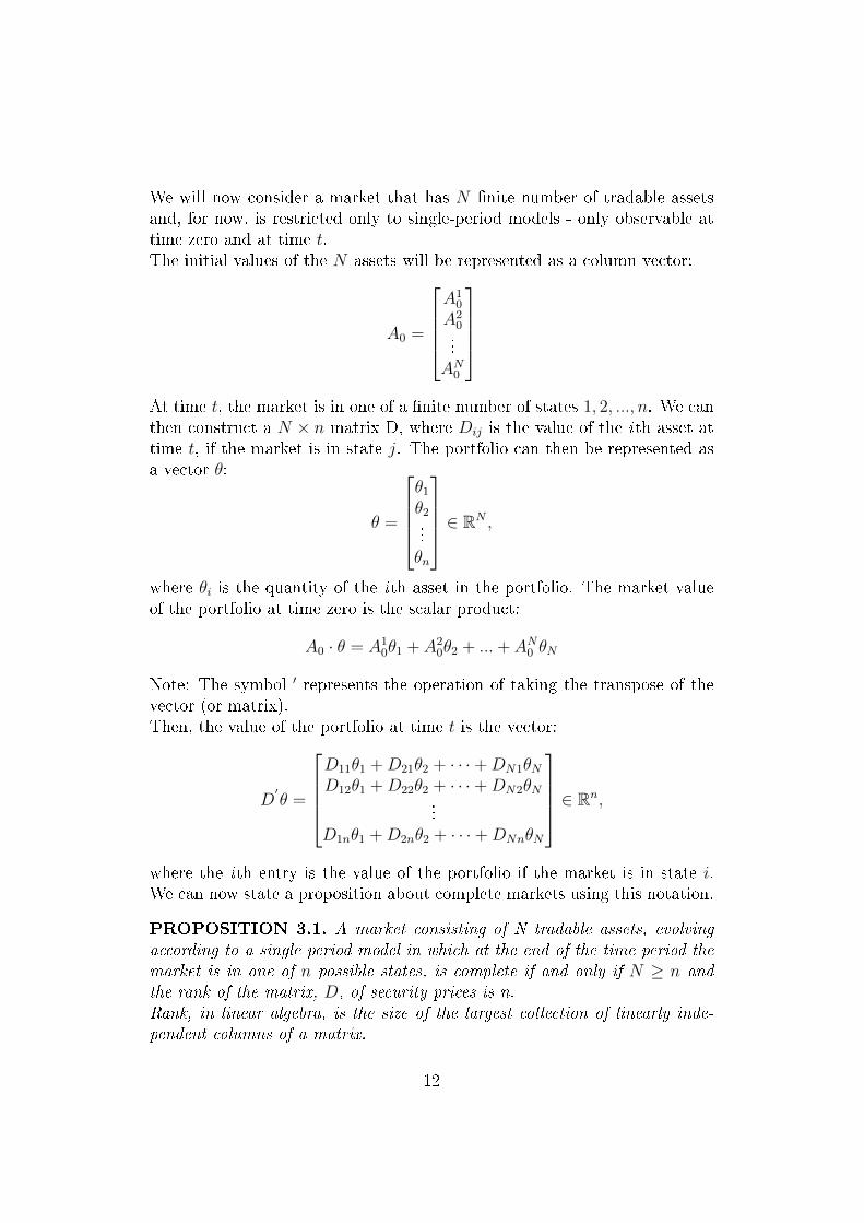
We will now consider a market that has N nite number of tradable assetsand, for now, is restricted only to single-period models - only observable attime zero and at time t.The initial values of the N assets will be represented as a column vector:

A0 =

A1

0

A20...AN

0

At time t, the market is in one of a nite number of states 1, 2, ..., n. We canthen construct a N × n matrix D, where Dij is the value of the ith asset attime t, if the market is in state j. The portfolio can then be represented asa vector θ:

θ =

θ1

θ2...θn

∈ RN ,

where θi is the quantity of the ith asset in the portfolio. The market valueof the portfolio at time zero is the scalar product:

A0 · θ = A10θ1 + A2

0θ2 + ...+ AN0 θN

Note: The symbol ′ represents the operation of taking the transpose of thevector (or matrix).Then, the value of the portfolio at time t is the vector:

D′θ =

D11θ1 +D21θ2 + · · ·+DN1θND12θ1 +D22θ2 + · · ·+DN2θN

...D1nθ1 +D2nθ2 + · · ·+DNnθN

∈ Rn,

where the ith entry is the value of the portfolio if the market is in state i.We can now state a proposition about complete markets using this notation.

PROPOSITION 3.1. A market consisting of N tradable assets, evolvingaccording to a single period model in which at the end of the time period themarket is in one of n possible states, is complete if and only if N ≥ n andthe rank of the matrix, D, of security prices is n.Rank, in linear algebra, is the size of the largest collection of linearly inde-pendent columns of a matrix.

12

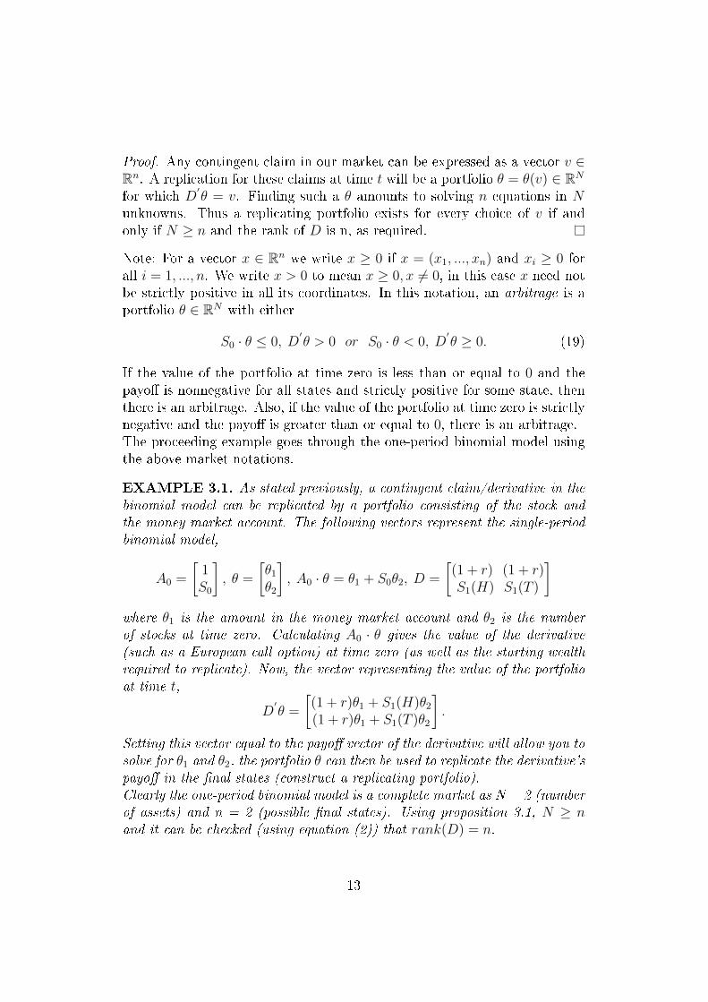
Proof. Any contingent claim in our market can be expressed as a vector v ∈Rn. A replication for these claims at time t will be a portfolio θ = θ(v) ∈ RN

for which D′θ = v. Finding such a θ amounts to solving n equations in N

unknowns. Thus a replicating portfolio exists for every choice of v if andonly if N ≥ n and the rank of D is n, as required.

Note: For a vector x ∈ Rn we write x ≥ 0 if x = (x1, ..., xn) and xi ≥ 0 forall i = 1, ..., n. We write x > 0 to mean x ≥ 0, x 6= 0, in this case x need notbe strictly positive in all its coordinates. In this notation, an arbitrage is aportfolio θ ∈ RN with either

S0 · θ ≤ 0, D′θ > 0 or S0 · θ < 0, D

′θ ≥ 0. (19)

If the value of the portfolio at time zero is less than or equal to 0 and thepayo is nonnegative for all states and strictly positive for some state, thenthere is an arbitrage. Also, if the value of the portfolio at time zero is strictlynegative and the payo is greater than or equal to 0, there is an arbitrage.The proceeding example goes through the one-period binomial model usingthe above market notations.

EXAMPLE 3.1. As stated previously, a contingent claim/derivative in thebinomial model can be replicated by a portfolio consisting of the stock andthe money market account. The following vectors represent the single-periodbinomial model,

A0 =

[1S0

], θ =

[θ1

θ2

], A0 · θ = θ1 + S0θ2, D =

[(1 + r) (1 + r)S1(H) S1(T )

]where θ1 is the amount in the money market account and θ2 is the numberof stocks at time zero. Calculating A0 · θ gives the value of the derivative(such as a European call option) at time zero (as well as the starting wealthrequired to replicate). Now, the vector representing the value of the portfolioat time t,

D′θ =

[(1 + r)θ1 + S1(H)θ2

(1 + r)θ1 + S1(T )θ2

].

Setting this vector equal to the payo vector of the derivative will allow you tosolve for θ1 and θ2, the portfolio θ can then be used to replicate the derivative'spayo in the nal states (construct a replicating portfolio).Clearly the one-period binomial model is a complete market as N = 2 (numberof assets) and n = 2 (possible nal states). Using proposition 3.1, N ≥ nand it can be checked (using equation (2)) that rank(D) = n.

13

The market described thus far has only one period, now we briey turn ourattention to a market with multiple periods.

Based on how we've dene the above market one would think that a multi-period model would not be complete. Suppose for example we have a ten-period binomial model, at time ten we would have 210 = 1024 nal states forour stock price. By proposition 3.1, we would need at least that many inde-pendent assets for our market to be complete. This isn't as big of a problemas it may seem as in Theorem 2.1 (replication of the multi-period binomialmodel) we dened ∆n to be an adapted portfolio process. What this meansis that the replicating portfolio is rebalanced after each time period - usingonly the two assets (in our case the stock and money market account). Therebalancing can only involve the purchasing more of one asset and the saleof the other asset - no money can be added or taken out. This is known asthe self-nancing property of the replicating portfolio.

So far we've considered markets that are complete, but what about an ex-ample of an incomplete market?

4 The Trinomial Model

The one-period trinomial model diers from the binomial model in that theunderlying asset, the stock, can take an intermediate price between uS0 anddS0, we will refer to this value as mS0. Note that only d < m < u needsto be true, it may not be the case that m = 1. In the binomial model weused H and T to represent an imaginary coin toss, for the trinomial modelwe introduce M to indicate that the stock at time one took the intermediatepath. The following gure shows the one-period trinomial model:

S0

S1(H) = uS0

S1(M) = mS0

S1(T ) = dS0

Figure 4: One-period trinomial model

Another major dierence between the binomial and trinomial models is thatthe trinomial model is an incomplete market - the nal states of a contingent

14

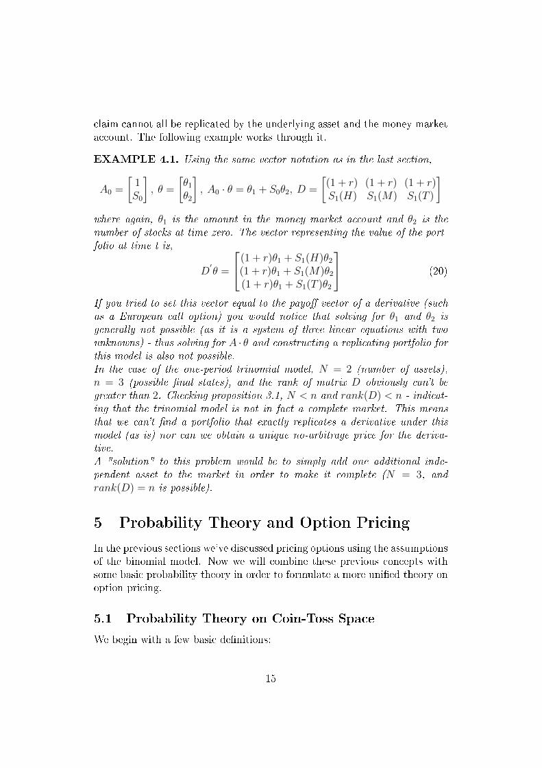
claim cannot all be replicated by the underlying asset and the money marketaccount. The following example works through it.

EXAMPLE 4.1. Using the same vector notation as in the last section,

A0 =

[1S0

], θ =

[θ1

θ2

], A0 · θ = θ1 + S0θ2, D =

[(1 + r) (1 + r) (1 + r)S1(H) S1(M) S1(T )

]where again, θ1 is the amount in the money market account and θ2 is thenumber of stocks at time zero. The vector representing the value of the port-folio at time t is,

D′θ =

(1 + r)θ1 + S1(H)θ2

(1 + r)θ1 + S1(M)θ2

(1 + r)θ1 + S1(T )θ2

(20)

If you tried to set this vector equal to the payo vector of a derivative (suchas a European call option) you would notice that solving for θ1 and θ2 isgenerally not possible (as it is a system of three linear equations with twounknowns) - thus solving for A · θ and constructing a replicating portfolio forthis model is also not possible.In the case of the one-period trinomial model, N = 2 (number of assets),n = 3 (possible nal states), and the rank of matrix D obviously can't begreater than 2. Checking proposition 3.1, N < n and rank(D) < n - indicat-ing that the trinomial model is not in fact a complete market. This meansthat we can't nd a portfolio that exactly replicates a derivative under thismodel (as is) nor can we obtain a unique no-arbitrage price for the deriva-tive.A "solution" to this problem would be to simply add one additional inde-pendent asset to the market in order to make it complete (N = 3, andrank(D) = n is possible).

5 Probability Theory and Option Pricing

In the previous sections we've discussed pricing options using the assumptionsof the binomial model. Now we will combine these previous concepts withsome basic probability theory in order to formulate a more unied theory onoption pricing.

5.1 Probability Theory on Coin-Toss Space

We begin with a few basic denitions:

15

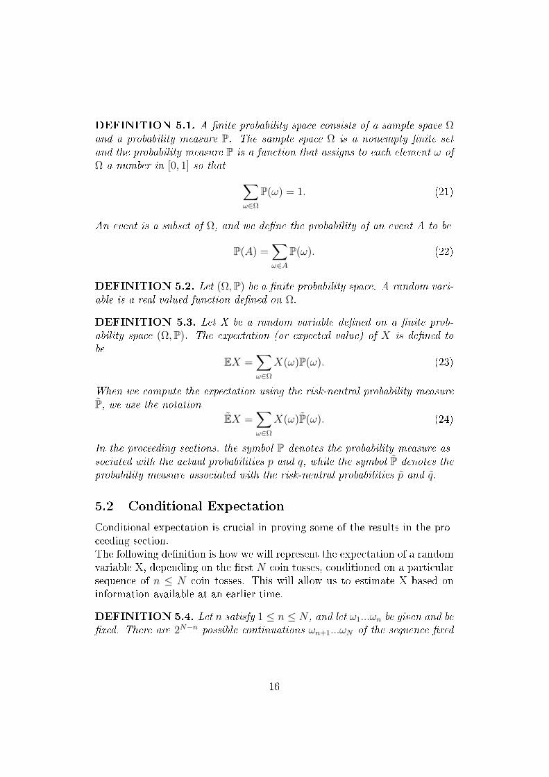
DEFINITION 5.1. A nite probability space consists of a sample space Ωand a probability measure P. The sample space Ω is a nonempty nite setand the probability measure P is a function that assigns to each element ω ofΩ a number in [0, 1] so that ∑

ω∈Ω

P(ω) = 1. (21)

An event is a subset of Ω, and we dene the probability of an event A to be

P(A) =∑ω∈A

P(ω). (22)

DEFINITION 5.2. Let (Ω,P) be a nite probability space. A random vari-able is a real-valued function dened on Ω.

DEFINITION 5.3. Let X be a random variable dened on a nite prob-ability space (Ω,P). The expectation (or expected value) of X is dened tobe

EX =∑ω∈Ω

X(ω)P(ω). (23)

When we compute the expectation using the risk-neutral probability measureP, we use the notation

EX =∑ω∈Ω

X(ω)P(ω). (24)

In the proceeding sections, the symbol P denotes the probability measure as-sociated with the actual probabilities p and q, while the symbol P denotes theprobability measure associated with the risk-neutral probabilities p and q.

5.2 Conditional Expectation

Conditional expectation is crucial in proving some of the results in the pro-ceeding section.The following denition is how we will represent the expectation of a randomvariable X, depending on the rst N coin tosses, conditioned on a particularsequence of n ≤ N coin tosses. This will allow us to estimate X based oninformation available at an earlier time.

DEFINITION 5.4. Let n satisfy 1 ≤ n ≤ N , and let ω1...ωn be given and bexed. There are 2N−n possible continuations ωn+1...ωN of the sequence xed

16

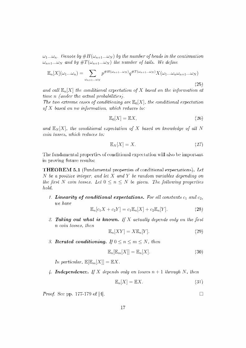
ω1...ωn. Denote by #H(ωn+1...ωN) by the number of heads in the continuationωn+1...ωN and by #T (ωn+1...ωN) the number of tails. We dene

En[X](ω1...ωn) =∑

ωn+1...ωN

p#H(ωn+1...ωN )q#T (ωn+1...ωN )X(ω1...ωnωn+1...ωN)

(25)and call En[X] the conditional expectation of X based on the information attime n (under the actual probabilities).The two extreme cases of conditioning are E0[X], the conditional expectationof X based on no information, which reduces to:

E0[X] = EX, (26)

and EN [X], the conditional expectation of X based on knowledge of all Ncoin tosses, which reduces to:

EN [X] = X. (27)

The fundamental properties of conditional expectation will also be importantin proving future results:

THEOREM 5.1 (Fundamental properties of conditional expectations). LetN be a positive integer, and let X and Y be random variables depending onthe rst N coin tosses. Let 0 ≤ n ≤ N be given. The following propertieshold.

1. Linearity of conditional expectations. For all constants c1 and c2,we have

En[c1X + c2Y ] = c1En[X] + c2En[Y ]. (28)

2. Taking out what is known. If X actually depends only on the rstn coin tosses, then

En[XY ] = XEn[Y ]. (29)

3. Iterated conditioning. If 0 ≤ n ≤ m ≤ N , then

En[Em[X]] = En[X]. (30)

In particular, E[Em[X]] = EX.

4. Independence. If X depends only on tosses n+ 1 through N , then

En[X] = EX. (31)

Proof. See pp. 177-179 of [4].

17

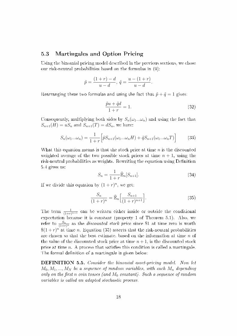
5.3 Martingales and Option Pricing

Using the binomial pricing model described in the previous sections, we choseour risk-neutral probabilities based on the formulas in (9):

p =(1 + r)− du− d

, q =u− (1 + r)

u− d.

Rearranging these two formulas and using the fact that p+ q = 1 gives:

pu+ qd

1 + r= 1. (32)

Consequently, multiplying both sides by Sn(ω1...ωn) and using the fact thatSn+1(H) = uSn and Sn+1(T ) = dSn, we have:

Sn(ω1...ωn) =1

1 + r

[pSn+1(ω1...ωnH) + qSn+1(ω1...ωnT )

](33)

What this equation means is that the stock price at time n is the discountedweighted average of the two possible stock prices at time n + 1, using therisk-neutral probabilities as weights. Rewriting the equation using Denition5.4 gives us:

Sn =1

1 + rEn[Sn+1]. (34)

If we divide this equation by (1 + r)n, we get:

Sn

(1 + r)n= En

[ Sn+1

(1 + r)n+1

]. (35)

The term 1(1+r)n+1 can be written either inside or outside the conditional

expectation because it is constant (property 1 of Theorem 5.1). Also, werefer to Sn

(1+r)nas the discounted stock price since $1 at time zero is worth

$(1 + r)n at time n. Equation (35) asserts that the risk-neutral probabilitiesare chosen so that the best estimate, based on the information at time n ofthe value of the discounted stock price at time n+ 1, is the discounted stockprice at time n. A process that satises this condition is called a martingale.The formal denition of a martingale is given below:

DEFINITION 5.5. Consider the binomial asset-pricing model. Now letM0,M1, ...,MN be a sequence of random variables, with each Mn dependingonly on the rst n coin tosses (and M0 constant). Such a sequence of randomvariables is called an adapted stochastic process.

18

1. IfMn = En[Mn+1], n = 0, 1, ..., N − 1, (36)

we say this process is a martingale.

2. IfMn ≤ En[Mn+1], n = 0, 1, ..., N − 1,

we say the process is a submartingale (even though it may have a ten-dency to increase);

3. IfMn ≥ En[Mn+1], n = 0, 1, ..., N − 1,

we say the process is a supermartingale (even though it may have atendency to decrease).

The following are a few useful properties of martingales:

REMARK 5.1. The martingale property in (36) of the previous denitionis a "one-step-ahead" condition. However, it implies a similar condition forany number of steps. If M0,M1, ...,MN is a martingale and n ≤ N − 2, thenthe martingale property (36) implies

Mn+1 = En+1[Mn+2].

Taking conditional expectation on both sides based on the information at timen and using property 3 of Theorem 5.1, we get

En[Mn+1] = En[En+1[Mn+2]] = En[Mn+2]

Because of (36), we have the "two-step-ahead" property

Mn = En[Mn+2].

Iterating this, argument, whenever 0 ≤ n ≤ m ≤ N , we have the "multistep-ahead" property,

Mn = En[Mm]. (37)

REMARK 5.2. The expectation of a martingale is constant over time, i.e.,if M0,M1, ...,MN is a martingale, then

M0 = EMn, n = 0, 1, ..., N. (38)

19

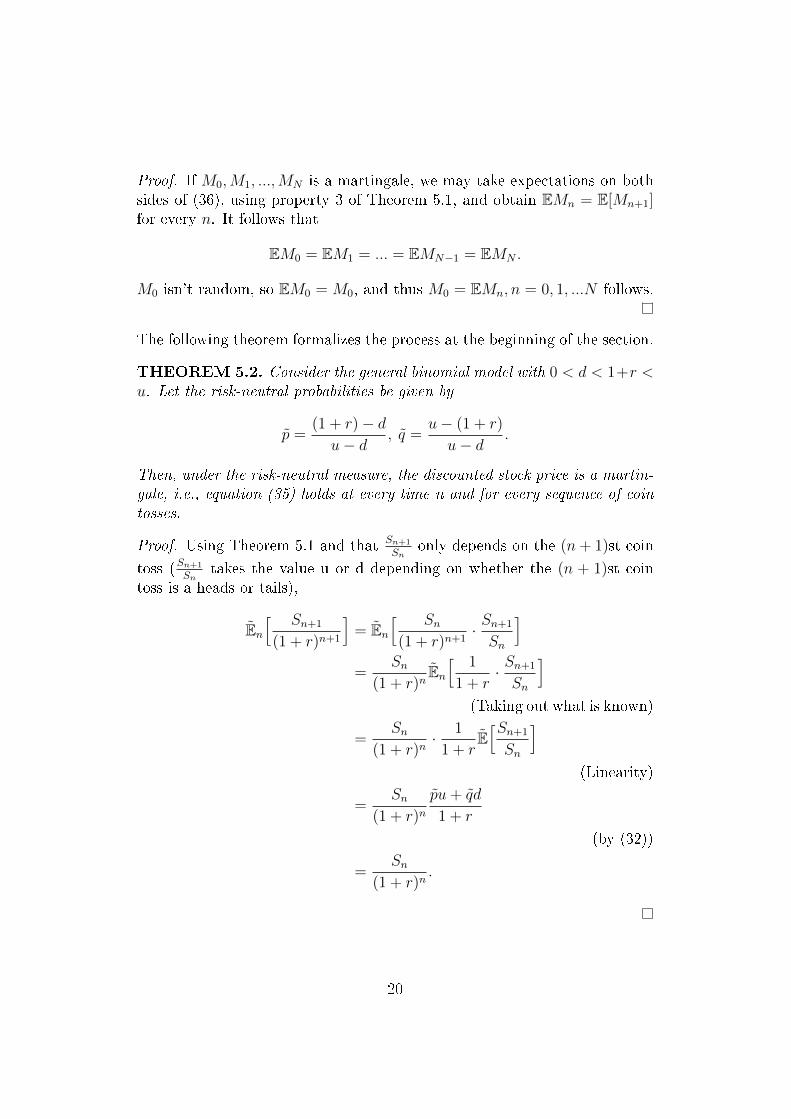
Proof. If M0,M1, ...,MN is a martingale, we may take expectations on bothsides of (36), using property 3 of Theorem 5.1, and obtain EMn = E[Mn+1]for every n. It follows that

EM0 = EM1 = ... = EMN−1 = EMN .

M0 isn't random, so EM0 = M0, and thus M0 = EMn, n = 0, 1, ...N follows.

The following theorem formalizes the process at the beginning of the section.

THEOREM 5.2. Consider the general binomial model with 0 < d < 1+r <u. Let the risk-neutral probabilities be given by

p =(1 + r)− du− d

, q =u− (1 + r)

u− d.

Then, under the risk-neutral measure, the discounted stock price is a martin-gale, i.e., equation (35) holds at every time n and for every sequence of cointosses.

Proof. Using Theorem 5.1 and that Sn+1

Snonly depends on the (n+ 1)st coin

toss (Sn+1

Sntakes the value u or d depending on whether the (n + 1)st coin

toss is a heads or tails),

En

[ Sn+1

(1 + r)n+1

]= En

[ Sn

(1 + r)n+1· Sn+1

Sn

]=

Sn

(1 + r)nEn

[ 1

1 + r· Sn+1

Sn

](Taking out what is known)

=Sn

(1 + r)n· 1

1 + rE[Sn+1

Sn

](Linearity)

=Sn

(1 + r)npu+ qd

1 + r

(by (32))

=Sn

(1 + r)n.

20

At the end of the binomial section, we discussed how under the risk-neutralprobabilities, the average rate of growth of a portfolio consisting of assets inthe stock and money markets equals the rate of growth of the money marketaccount. So, as stated previously, the average rate of growth of an investorswealth is equal to the interest rate, r.This result is explained in the following theorem, which states that the wealthprocess is also a martingale.

THEOREM 5.3. Consider the binomial model with N periods.Let ∆0,∆1, ...,∆N−1 be an adapted portfolio (as mentioned previously), let X0

be a real number, and let the wealth process X1, ..., XN be generated recursivelyby (14), the wealth equation:

Xn+1 = ∆nSn+1 + (1 + r)(Xn −∆nSn).

. Then the discounted wealth process Xn

(1+r)n, n = 0, 1, ..., N, is a martingale

under the risk-neutral measure; i.e,

Xn

(1 + r)n= En

[ Xn+1

(1 + r)n+1

], n = 0, 1, ..., N − 1. (39)

Proof.

En

[ Xn+1

(1 + r)n+1

]= En

[ ∆nSn+1

(1 + r)n+1+Xn −∆nSn

(1 + r)n

]= En

[ ∆nSn+1

(1 + r)n+1

]+ En

[Xn −∆nSn

(1 + r)n

](Linearity)

= ∆nEn

[ Sn+1

(1 + r)n+1

]+Xn −∆nSn

(1 + r)n

(Taking out what is known)

= ∆nSn

(1 + r)n+Xn −∆nSn

(1 + r)n

(Theorem 5.2)

=Xn

(1 + r)n.

COROLLARY 5.1. Under the conditions of Theorem 5.3, we have

E[ Xn

(1 + r)n

]= X0, n = 0, 1, ..., N. (40)

21

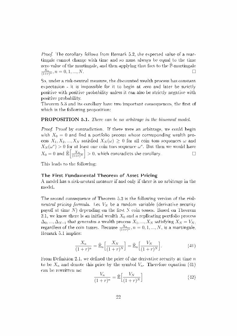
Proof. The corollary follows from Remark 5.2, the expected value of a mar-tingale cannot change with time and so must always be equal to the timezero value of the martingale, and then applying that fact to the P-martingale

Xn

(1+r)n, n = 0, 1, ..., N .

So, under a risk-neutral measure, the discounted wealth process has constantexpectation - it is impossible for it to begin at zero and later be strictlypositive with positive probability unless it can also be strictly negative withpositive probability.Theorem 5.3 and its corollary have two important consequences, the rst ofwhich is the following proposition:

PROPOSITION 5.1. There can be no arbitrage in the binomial model.

Proof. Proof by contradiction. If there were an arbitrage, we could beginwith X0 = 0 and nd a portfolio process whose corresponding wealth pro-cess X1, X2, ..., XN satised XN(ω) ≥ 0 for all coin toss sequences ω andXN(ω∗) > 0 for at least one coin toss sequence ω∗. But then we would have

X0 = 0 and E[

XN

(1+r)N

]> 0, which contradicts the corollary.

This leads to the following:

The First Fundamental Theorem of Asset Pricing

A model has a risk-neutral measure if and only if there is no arbitrage in themodel.

The second consequence of Theorem 5.3 is the following version of the risk-neutral pricing formula. Let VN be a random variable (derivative securitypayo at time N) depending on the rst N coin tosses. Based on Theorem2.1, we know there is an initial wealth X0 and a replicating portfolio process∆0, ...,∆N−1 that generates a wealth process X1, ..., XN satisfying XN = VN ,regardless of the coin tosses. Because Xn

(1+r)n, n = 0, 1, ..., N , is a martingale,

Remark 5.1 implies:

Xn

(1 + r)n= En

[ XN

(1 + r)N

]= En

[ VN(1 + r)N

]. (41)

From Denition 2.1, we dened the price of the derivative security at time nto be Xn and denote this price by the symbol Vn. Therefore equation (41)can be rewritten as:

Vn(1 + r)n

= E[ VN

(1 + r)N

](42)

22

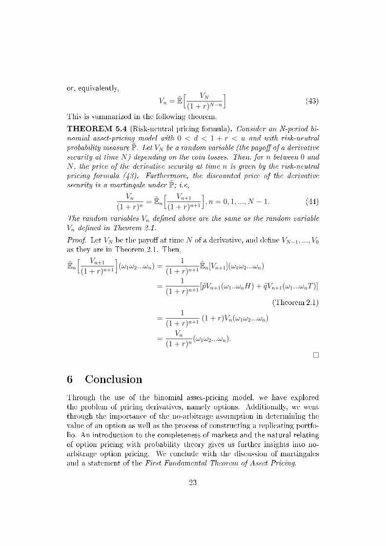
or, equivalently,

Vn = E[ VN

(1 + r)N−n

](43)

This is summarized in the following theorem.

THEOREM 5.4 (Risk-neutral pricing formula). Consider an N-period bi-nomial asset-pricing model with 0 < d < 1 + r < u and with risk-neutralprobability measure P. Let VN be a random variable (the payo of a derivativesecurity at time N) depending on the coin tosses. Then, for n between 0 andN , the price of the derivative security at time n is given by the risk-neutralpricing formula (43). Furthermore, the discounted price of the derivativesecurity is a martingale under P; i.e,

Vn(1 + r)n

= En

[ Vn+1

(1 + r)n+1

], n = 0, 1, ..., N − 1. (44)

The random variables Vn dened above are the same as the random variableVn dened in Theorem 2.1.

Proof. Let VN be the payo at time N of a derivative, and dene VN−1, ..., V0

as they are in Theorem 2.1. Then,

En

[ Vn+1

(1 + r)n+1

](ω1ω2...ωn) =

1

(1 + r)n+1En[Vn+1](ω1ω2...ωn)

=1

(1 + r)n+1[pVn+1(ω1..ωnH) + qVn+1(ω1...ωnT )]

(Theorem 2.1)

=1

(1 + r)n+1(1 + r)Vn(ω1ω2...ωn)

=Vn

(1 + r)n(ω1ω2...ωn).

6 Conclusion

Through the use of the binomial asset-pricing model, we have exploredthe problem of pricing derivatives, namely options. Additionally, we wentthrough the importance of the no-arbitrage assumption in determining thevalue of an option as well as the process of constructing a replicating portfo-lio. An introduction to the completeness of markets and the natural relatingof option pricing with probability theory gives us further insights into no-arbitrage option pricing. We conclude with the discussion of martingalesand a statement of the First Fundamental Theorem of Asset Pricing.

23

References

[1] Avellaneda, M. and Laurence, P. Quantitative Modeling of DerivativeSecurities. Chapman & Hall/CRC, Boca Raton, 2000.

[2] Billingsley, R. Understanding Arbitrage: An Intuitive Approach to Fi-nancial Analysis. FT Press, 2005.

[3] Etheridge, A. A Course in Financial Calculus. Cambridge UniversityPress, Cambridge, 2002.

[4] Shreve, S. Stochastic Calculus for Finance, Vol. I: The Binomial AssetPricing Model. Springer Finance. Springer, New York, 2004.

24