Arbitrage Pricing Theory for Idiosyncratic Variance

Factors

PRELIMINARY AND INCOMPLETE: PLEASE DO NOT CITE WITHOUT

PERMISSION

Eric Renault∗, Thijs van der Heijden†, and Bas J.M. Werker‡

February 7, 2016

Abstract

Recent research has documented the existence of common factors in individual

asset’s idiosyncratic variances or squared idiosyncratic returns. We provide an

Arbitrage Pricing Theory that leads to a linear factor structure for prices of squared

excess returns. This pricing representation allows us to study the interplay of factors

at the return level with those in idiosyncratic variances. We document the presence

of a common volatility factors. Linear returns do not have exposure to this factor

when using at least five principal components as linear factors. The price of the

common volatility factor is zero.

JEL codes : C58, G12.

Key words and phrases: Common volatility factors, Option prices.

∗Department of Economics, Brown University, 64 Waterman Street, Providence RI 02912, USA, email:eric renault@brown.edu†Department of Finance, The University of Melbourne, 198 Berkeley Street, Carlton VIC 3010, Aus-

tralia, email: thijsv@unimelb.edu.au‡Econometrics and Finance Group, Netspar, Tilburg University, P.O. Box 90153, 5000 LE, Tilburg,

The Netherlands. E-mail: Werker@TilburgUniversity.edu. We thank conference participants at theEconometrics of High-Dimensional Risk Networks at the Stefanovich Center and seminar participants atTilburg University for helpful comments and suggestions.

1

1 Introduction

Recently, several papers have documented the presence of a common factor in idiosyn-

cratic volatilities from a linear return factor model, arguing that this factor is priced which

would be at odds with standard theory. This line of research started with Ang, Hodrick,

Xing, and Zhang (2006) who coined their result the “idiosyncratic volatility puzzle”.

Recent contributions are Duarte, Kamara, Siegel, and Sun (2014) and Herskovic, Kelly,

Lustig, and Van Nieuwerburgh (2016). In the present paper, we revisit this puzzle within

the Ross (1976) Arbitrage Pricing Theory (APT) framework. Specifically, we propose a

different formulation of the classical APT in terms of (cumulative) portfolios of assets

in the economy. Intuitively, our formulation can be viewed as a transposed version of

standard continuous-time finance theory, where the index of the stochastic process refers

to an asset index rather than time.

The theoretical advantage of our approach is twofold. On the one hand, by considering

economies with a continuum of assets, we share, with Al-Najjar (1998)’s seminal work, the

advantage that we can replace the traditional conclusion of APT “most assets have small

pricing errors” by the more testable statement that “outside a set of Lebesgue measure

zero, every asset is exactly factor-priced”. Our framework will be shown to encompass

the concept of approximate factor structure recently put forward by Gagliardini, Ossola,

and Scaillet (2014). On the other hand, our approach in terms of stochastic processes

(where the continuous “time” index is actually an index for a specific portfolio) allows

us to resort to the theory of quadratic variations and related tools. In short, our new

formulation of an approximate factor structure easily extends the APT for linear returns

to squared returns and thus to (idiosyncratic) volatilities.

In contrast to Ang, Hodrick, Xing, and Zhang (2006), Duarte, Kamara, Siegel, and

Sun (2014) and Herskovic, Kelly, Lustig, and Van Nieuwerburgh (2016), we do not study

idiosyncratic volatility as a possible missing factor in linear returns, but instead consider

the factor structure of squared returns directly. Our model predicts the presence of a

set of risk prices related to the squared linear factors as well as to any additional factors

driving the idiosyncratic variances. This allows us to disentangle the effect of possibly

omitted factors at the linear return level from possible factors in idiosyncratic variances.

On the one hand, if a factor is forgotten in the factor pricing of linear returns, obviously

its squared value will show up as a common factor of idiosyncratic volatilities. However,

there is no argument, either theoretical or empirical, that prevents new factors (i.e.,

unrelated to the factors at the linear return level) to show up in idiosyncratic variances.

In our empirical analysis of S&P500 index firms over the period 1996-2013, we doc-

ument the presence of a common factor in idiosyncratic variances in addition to (the

squares of) the factors in the linear excess returns. We extract up to ten factors of the

linear return model using principal components and analyze the factor structure of the

2

squared residual (idiosyncratic) returns. We then include both the linear factors and

the squared return factor in a Fama and MacBeth (1973) analysis. The squared return

factor has some incremental explanatory power in the linear return model even with ten

principal components included. However, the loadings on the squared return factor are

insignificantly different from zero when ten principal components are included. However,

the focus of our paper to document whether the price of risk of the squared return fac-

tor is, economically and statistically, different from zero. We therefore focus on excess

squared excess returns, i.e., squared excess returns minus their price. In order to con-

struct these excess squared excess returns, we compute the price of squared excess returns

using the spanning results of Bakshi and Madan (2000). They show that the price of any

payoff that is a twice-differentiable function of the underlying security value is given by a

combination of a position in a risk-free asset, a forward contract and a suitable portfolio

of put and call options. By using this set of excess squared excess returns, we are able to

check that, irrespective of the number of principal components that are included (namely

5 or 10), the price of risk of the squared return factor is insignificantly different from

zero . This is in contrast to the same analysis that uses the five Fama and French (2015)

factors, where both the average loading and the price of risk of the squared return factor

are significantly different from zero. The squared return factor also has a substantially

higher explanatory power for linear returns in the Fama and French (2015) case than

when using principal components.

In order to understand our results, it is useful to distinguish the concepts of statistical

and financial factor models. In a statistical factor model one extracts (e.g., using principal

components) factors such that the residuals become cross-sectionally uncorrelated, i.e.,

diversifiable. In a financial factor model, one extracts factors (e.g., the Fama-French fac-

tors) such that the residuals become idiosyncratic in the sense that they do not command

a risk premium, i.e., have zero price. The Arbitrage Pricing Theory states that, under an

additional no-arbitrage assumption, a statistical factor model implies a financial factor

model. The converse, however, does not hold. That is, there may exist non-diversifiable

risks that do not command a risk premium, i.e., have zero price. Thus, using Fama-

French factors at the linear return level, may leave a common (non-diversifiable) factor

in the “idiosyncratic” residuals. The square of this factor will show as a common factor

in the “idiosyncratic” variances and it may or may not be priced. The contribution of

the present paper is to show that, in line with the intuition that diversifiable risk cannot

command any risk premium, the use of a statistical factor model at the linear return

level, still leads to a common factor in idiosyncratic variances, but we empirically find

this common factor to be idiosyncratic in the sense that it has zero price.

Our empirical results shed new light on the idiosyncratic volatility puzzle in at least

three respects. First, in contrast with several papers in the extant literature, our focus

of interest is beyond the role of possible forgotten factors in the linear factor model of

3

standard asset returns. By using up to ten principal components, we make sure that

no common statistical factor is missing and we still find a common factor in squared

idiosyncratic residuals. Obviously, this common factor captures less (about ten percent)

of the total variance of squared residuals than when using Fama-French type factors.

In the latter case, people find numbers up to 30 percent or more. See, e.g., Duarte,

Kamara, Siegel, and Sun (2014) and Herskovic, Kelly, Lustig, and Van Nieuwerburgh

(2016). Second, since volatility is an important determinant of option prices, our paper

is also related to the literature on the factor structure in option prices, e.g., Christoffersen,

Fournier, and Jacobs (2015). Instead of studying factor structures in option prices, we

use these option prices to obtain a price of squared excess returns. As follows from

our theory, this price of a quadratic transformation is much more easily studied in an

Arbitrage Pricing Theory framework than the more complicated non-linearities in option

prices. Third, our paper is also related to the literature on skewness in asset pricing,

which started with Kraus and Litzenberger (1976) showing that investors exhibiting non-

increasing absolute risk aversion is equivalent to an extension of the standard Capital

Asset Pricing Model that incorporates skewness as the covariance between asset returns

and the squared market return. Harvey and Siddique (2000) focus on the cross-section

of expected returns and use conditional rather than unconditional skewness. They write

down a model in which the pricing kernel is linear in the market return and its square.

Chabi-Yo, Leisen, and Renault (2014) study the aggregation of preferences in the presence

of skewness risk and show how the risk premium for skewness is linked to the portfolio

that optimally hedges the squared market return. However, since this hedge is not perfect,

an additional factor may appear in case of heterogeneous preferences for skewness. In

other words, the results of Chabi-Yo, Leisen, and Renault (2014) provide some structural

underpinnings to our working hypothesis that, in case of a linear factor model, investors’

preferences may lead to not only the squared market return as a factor, but also an

additional one due to the tracking error on the squared market return.

The remainder of the paper is structured as follows. In Section 2, we propose a

new formulation of the APT model for linear returns. We use this new formulation,

in Section 3, to study an approximate factor structure in excess squared excess returns

(i.e., idiosyncratic variances) and derive testable implications. In Section 4 we describe

the sample and the variables we construct. Section 5 contains the empirical results and

Section 6 concludes.

2 The APT revisited

We start our theoretical analysis by providing a new proof of the classical Arbitrage

Pricing Theory (APT). Instead of, e.g., Al-Najjar (1998) and Gagliardini, Ossola, and

Scaillet (2014), we consider cumulative portfolios of assets to obtain the APT. A precise

4

link with existing APT results is provided in Remark 1 below. The advantage of our

approach is that it readily extends to common factors in idiosyncratic variances, the

main topic of this paper. At the level of linear returns there is not much new.

Consider n traded assets with (arithmetically compounded) excess returns R(n)i , i =

1, . . . , n. Recall that excess returns have price zero, i.e., they refer to zero-investment

opportunities. In this paper we actually call any investment with zero price an excess

return.

In order to formalize the assumption of an approximate factor structure, we construct

cumulative portfolios. That is, for given u ∈ [0, 1], we construct an equally weighted port-

folio consisting of 1/n exposures in the first u fraction of the assets.1 Such a cumulative

portfolio thus has excess return

R(n)(u) =1

n

bunc∑i=1

R(n)i . (1)

Note that R(n)(u) is simply an alternative representation of the available assets R(n)i in

the market. We have R(n)(0) = 0 and R(n)(1) represents an equally weighted portfolio in

all available assets in the economy. Formally, R(n) is a stochastic process in D[0, 1], the

set of cadlag functions on [0, 1], equipped with the supremum norm ‖·‖. All convergences

of stochastic processes in this paper are weak convergence in (D[0, 1], ‖·‖).The rewrite from original assets with excess returns R

(n)i to portfolios indexed by

u ∈ [0, 1] facilitates a formal analysis of factor models. Observe that in the definition

below, no moment restrictions are imposed on the excess returns, the factors, or the

idiosyncratic errors.2

Definition 1 The (sequence of) excess return process(es) R(n) is said to satisfy an ap-

proximate factor structure if there exists a K-dimensional (random) factor F and deter-

ministic finite-variation functions α and β such that we may write

R(n)(u) =

∫ u

0

α(v)dv +

∫ u

0

βᵀ(v)dvF + Z(n)(u), (2)

where Z(n) converges to zero.

Our formulation of a factor model is, technically, of a different nature than existing

results in the literature. The following remark shows that our setup encompasses recently

proposed alternatives.

1In Remark 1 we extend this to non-equally weighted portfolios.2In particular, it is not even assumed at this stage that the errors Z(n) and the factor F are uncor-

related; see Remark 5.

5

Remark 1 Several other formalizations of the classical APT result exist in the literature,

e.g., Gagliardini, Ossola, and Scaillet (2014) and Al-Najjar (1998). Those papers often

start from sequences of excess returns written as

R(n)i = α

(n)i + β

(n)ᵀi F + ε

(n)i , (3)

with Eε(n)i = 0. Now, portfolios with excess returns R(n)(u) can be defined as above. The

setting in Gagliardini, Ossola, and Scaillet (2014) is arguably more general in the sense

that the portfolios considered are not necessarily equally weighted. This can be included

in our setting by considering weights δ(n)i > 0 satisfying

n∑i=1

δ(n)i = 1, (4)

n

n∑i=1

(δ

(n)i

)2

= O(1). (5)

The condition that the weights δ(n)i sum to one is made for convenience only and imma-

terial as we consider excess returns. The second condition is reminiscent of the concept

of bounded Asymptotic Quadratic Variation in Time (AQVT) introduced in Mykland and

Zhang (2006). To see that, note that the weights δ(n)i may be seen as the lengths of

consecutive intervals3 (∆(n)j−1,∆

(n)j ] in [0, 1], i.e.,

∆(n)j =

j∑i=1

δ(n)i , j = 1, . . . , n,

with ∆(n)0 = 0. These weights can be used to construct a continuum of portfolios much

like (1). More precisely we define

R(n)∆ (u) =

n∑i=1

R(n)i δ

(n)i 1

[∆(n)i ≤u]

. (6)

Note that conditions (4) and (5) are in particular fulfilled for the weights δ(n)i = 1/n,

leading to the equally weighted portfolio R(n)∆ (u) = R(n)(u). In general, R

(n)δ (u) is a

stochastic process (with sample paths in D[0, 1]), decomposes into

R(n)∆ (u) =

n∑i=1

α(n)i δ

(n)i 1

[∆(n)i ≤u]

+n∑i=1

β(n)ᵀi Fδ

(n)i 1

[∆(n)i ≤u]

+n∑i=1

ε(n)i δ

(n)i 1

[∆(n)i ≤u]

.

In order to satisfy Definition 1, we assume the existence of finite-variation functions α

3It is tempting to call the “time intervals”. However, note that the index u does not indicate timebut the fraction of assets included in a portfolio.

6

and β defined by

n∑i=1

α(n)i δ

(n)i 1

[∆(n)i ≤u]

→∫ u

0

α(v)dv (7)

n∑i=1

β(n)i δ

(n)i 1

[∆(n)i ≤u]

→∫ u

0

β(v)dv (8)

These conditions impose sufficient stability on the intercepts α and the factor loadings β.

Intuitively, these functions α and β are approximatively given by

u ∈ (∆(n)i−1,∆

(n)i ]⇒ α(u) ≈ α

(n)i and β(u) ≈ β

(n)i . (9)

The additional generality obtained by allowing non-equal weights may be, from a prac-

tical point of view, limited. Indeed, Theorem 1 below shows that they are not needed to

obtain the classical Arbitrage Pricing Theory. In order to keep in line with the existing

literature, we now show that they do play a role in the interpretation of assumptions

needed to get convergence to zero of the residual process

Z(n)∆ (u) =

n∑i=1

ε(n)i δ

(n)i 1

[∆(n)i ≤u]

.

One easily verifies

VarZ

(n)∆ (u)

≤ n

(n∑i=1

(δ

(n)i

)2)ρ(

Var[ε

(n)i

]ni=1

)n

,

where ρ(A) stands for the maximum eigenvalue of a symmetric matrix A. Now, Assump-

tion APR3 in Gagliardini, Ossola, and Scaillet (2014) is akin to assuming

ρ(

Var[ε

(n)i

]ni=1

)n

→ 0,

so that the AQVT assumption (5) implies

supu∈[0,1]

VarZ

(n)∆ (u)

→ 0.

As a result, the conditions in Definition 1 are satisfied.

In other words, up to reweighing that is immaterial in our setting as explained above,

our definition of approximate factor structure encompasses the setting of Gagliardini, Os-

sola, and Scaillet (2014) as a particular case. The convergence derived above corresponds

to Lemma 13 in Appendix 3 of Gagliardini, Ossola, and Scaillet (2014). They stress

7

that reweighing matters for them because it allows them to formalize the concept of a

block dependence structure. Such a structure may be empirically relevant, for instance,

in the case of unobserved industry specific factors that are independent among industries

. Since reweighing is mathematically immaterial in our setting, we will throughout focus

on equally weighted portfolios in our theoretical derivations.

It is worth acknowledging that some papers have documented within-industry correla-

tion patterns that point to industry-specific factors, compare, e.g., Ait-Sahalia and Xiu

(2015). From a statistical point of view, such industry factors present themselves in the

form of a block-diagonal covariance structure (in case assets are sorted by industry). The

question whether such industry factors should be included as market-wide factors is es-

sentially an empirical one. From a theoretical point of view, they should be included in

case the size of the industry relative to the total market does not vanish asymptotically.

Indeed, in that case the industry risk cannot be diversified.

Definition 1 formalizes our assumption of a factor structure. In order to illustrate

the more abstract results, we introduce an example that will also form the basis of our

empirical analysis later.

Example As we are particularly interested in the pricing of idiosyncratic variance fac-

tors, we consider a standard stochastic volatility model. For simplicity, we focus on a

single factor (K = 1). Consider

Ri = αi + βiF + (ωi + ϕiG)1/2 νi, (10)

for constants αi, βi, ωi, and ϕi and where G is a common positive volatility factor. We

assume that the νi’s are i.i.d. zero-mean random variables, independent of both F and

G, whose variances are normalized to unity. Moreover, we assume the ωi and ϕi to be

bounded away from zero and infinity.

Under the regularity conditions (7) and (8) on the α and β (in the context of equally

weighted portfolios, i.e., δ(n)i = 1/n), we get an approximate factor structure with

Z(n)(u) =1

n

bunc∑i=1

(ωi + ϕiG)1/2 νi + o (1) . (11)

Then, the functional law of large numbers gives the required convergence of the process

Z(n) to zero. Clearly, this result relies on the assumed cross-sectional independence of

the idiosyncratic errors νi. We will not provide details here as this law of large numbers

is an immediate consequence of the (functional) central limit theorem we apply to verify

the conditions of Definition 2 below.

8

In order to derive the APT pricing implications, we consider portfolios of the base

assets R(n)i , i = 1, . . . , n. Formally, we identify such a portfolio with a finite-variation

function h. This portfolio’s excess return is then, by definition,∫ 1

u=0

h(u)dR(n)(u). (12)

Taking h(u) = 1, we would find the excess return of an equally weighted portfolio with

exposures 1/n to all n assets. A value-weighted portfolio can be obtained by choosing

h(u) proportional to the relative market share of the u-th asset in the economy. As we

work with excess returns, note in particular that increments in R(n) are also excess returns

of portfolios consisting of a subset of the entire asset universe.

Remark 2 - Factor-mimicking portfolios If the excess returns R(n) satisfy an ap-

proximate factor structure, we can define a K-dimensional function H of finite variation

on [0, 1] such that ∫ 1

u=0

H(u)βᵀ(u)du = IK , (13)

the K ×K identity matrix. This is possible as long as the components of β are linearly

independent.4 Then the K portfolios induced by H, i.e.,

F =

∫ 1

u=0

H(u)dR(n)(u), (14)

can also be used as factors. To see that, note that (2) implies

F =

∫ 1

0

α(u)H(u)du+ F +

∫ 1

0

H(u)dZ(n)(u).

Hence, we may write, again using (2),

R(n)(u) =

∫ u

0

α(v)dv

+

∫ u

0

βᵀ(v)dv

[F −

∫ 1

0

α(w)H(w)dw −∫ 1

0

H(w)dZ(n)(w)

]+ Z(n)(u)

=

∫ u

0

[α(v)− βᵀ(v)

∫ 1

0

α(w)H(w)dw

]dv +

∫ u

0

βᵀ(v)dvF

+

[Z(n) −

∫ u

0

βᵀ(v)dv

∫ 1

0

H(w)dZ(n)(w)

],

where the last term indeed converges to zero. Observe that switching to factor mimicking

4Formally, the K components of the function H are obtained by Gramm-Schmidt orthogonalization(and normalization) of the linearly independent components of the function β using the scalar product

〈f, g〉 =∫ 1

0f(u)g(u)du.

9

portfolios in this way does not affect the factor loadings β, but the intercept α is affected.

Remark 3 - Repackaging An important point in theoretical foundations of the APT

is that its assumptions should be invariant under so-called “repackaging”, see, e.g., Al-

Najjar (1999). Loosely speaking this means that the assumptions should be invariant with

respect to reordering the assets and with respect to forming portfolios. It’s easy to see that

our Definition 1 indeed obeys to this invariance.

Consider first a reordering of the assets. Note that (2) implies, for given w ∈ [0, 1],

R(n)(u)−R(n)(w) =

∫ u

w

α(v)dv +

∫ u

w

βᵀ(v)dv + Z(n)(u)− Z(n)(w). (15)

Now consider p+1 fixed constants 0 = u0 < u1 < . . . < up = 1. A reordering of assets can

be obtained by permuting the p intervals [uj−1, uj], j = 1, . . . , p. It’s clear that reordering

the assets by pasting together the increments of the excess return processes R(n) over each

of the permuted intervals satisfies the conditions of Definition 1 in case the original excess

return processes R(n) do.

Secondly, consider forming portfolios of the available assets. This is formalized by a

fixed finite-variation function h∗ and by considering the excess return process∫ u

0h∗(v)dR(n)(v).

Such process obviously satisfies Definition 1 as soon as R(n) does. Indeed, we have, in

view of (2),∫ u

0

h∗(v)dR(n)(v) =

∫ u

0

h∗(v)α(v)dv +

∫ u

0

h∗(v)βᵀ(v)dv +

∫ u

0

h∗(v)dZ(n)(v),

using the same arguments as in the proof of Theorem 1, we find that the last term con-

verges to zero. Moreover, h∗α and h∗β are of finite variation (as the product of finite

variation functions). As a result,∫ u

0h∗(v)dR(n)(v) satisfies an approximate factor struc-

ture as well.

We can now state our version of the APT; its proof can be found in the appendix.

Theorem 1 Assume that the excess return process R(n) satisfies an approximate factor

structure. Furthermore, assume that there are no arbitrage opportunities in the sense that

it is not possible to construct a portfolio h whose excess return converges, as n→∞, to

a non-zero constant. Then there exists a K-dimensional vector with prices of risk λ such

that

α(u) = −β(u)ᵀλ, (16)

up to a set of Lebesgue measure zero.

We end this section’s recollection of the Arbitrage Pricing Theory with a few remarks.

These are not unique to our setting, but revisit some discussions in the vast literature on

the APT.

10

Remark 4 - Factor dimension and omitted factors

An important empirical question relates to the appropriate number of factors. We address

this question here from a theoretical point of view. We return to it, from an empirical

point of view, in Section 5.

First note that the relevant notion in Definition 1 is the space spanned by the (random)

components of F and the constant. Thus, we can always specify a vector F of factors

such that no linear combination of the components of F is deterministic, i.e., such that

the variance matrix of F is non-singular.5 However, this does not exclude that a strictly

smaller factor space would not also be valid. Indeed, assume that one of the components

of the factor loadings β is a linear combination of the other components; for instance

suppose that, for almost every u ∈ [0, 1], we have

β1(u) =K∑k=2

ζkβk(u).

In that case, we can also write down a K−1-dimensional factor structure using the factor

F defined by

F = [Fk + ζkF1]k=Kk=2 .

Therefore, we will maintain throughout the assumption that no linear combination of the

K components of F is deterministic and that no linear combination of the K components

of β is zero (a.e.). Under this maintained assumption, it is not possible to write an

approximate factor structure with less than K factors.

Conversely, it is useful to consider the situation of possibly omitted factors. So suppose

that the excess return process satisfies an approximate factor structure with factors (F, Fo),

i.e.,

R(n)(u) =

∫ u

0

α(v)dv +

∫ u

0

βᵀ(v)dvF +

∫ u

0

βᵀo (v)dvFo + Z(n)(u), (17)

where Z(n) converges to zero. Assume now that the researcher omits the factors Fo from

the analysis. This researcher effectively considers the “idiosyncratic” errors∫ u

0βᵀo (v)dvFo+

Z(n)(u). This will only converge to zero if βo = 0. Consequently, Definition 1 precisely

identifies the correct number of factors.

Remark 5 - Identification of factors

A subtle and sometimes overlooked point refers to the regression interpretation of a factor

model as assumed in Definition 1. Note that this definition does not impose orthogonality

of F and Z(n), but merely that the process Z(n) vanish asymptotically. Actually, observe

that orthogonality of factors and idiosyncratic terms is assumed in Gagliardini, Ossola,

and Scaillet (2014), though never used in their proofs. However, in case the convergence

5For sake of expositional simplicity we assume here that this variance matrix exists.

11

to zero of the process Z(n) is also uniform in L2, i.e.,

supu∈[0,1]

VarZ(n)(u)

→ 0,

we obtain by Cauchy-Schwartz

supu∈[0,1]

∣∣CovF,Z(n)(u)

∣∣→ 0. (18)

As, by definition,

Z(n)(u) ≈ 1

n

[un]∑i=1

R

(n)i − α

(n)i − β

(n)ᵀi F

=

1

n

[un]∑i=1

ε(n)i ,

it is natural to impose that ε(n)i is not correlated with F . In that case, we can interpret (2)

as a regression equation. Of course, (18) does not imply that ε(n)i is uncorrelated with

F for every individual asset i. It is however standard practice in the empirical literature

to assume the idiosyncratic errors to be uncorrelated with the factors for each individual

asset. We also impose this identifying condition in Section 5. However, note that this

practice has been criticized, going as far as questioning the testability of Ross (1976)’s

APT. Actually, the approach of characterizing the APT in an economy with a continuum

of assets, as in Al-Najjar (1998) and Gagliardini, Ossola, and Scaillet (2014), is pre-

cisely motivated by this criticism. Our paper addresses the issue by looking at cumulative

portfolios of assets.

Besides its conceptual relevance, Remark 5 also refers to the estimation of factor

models using time-series regressions. A criticism of single-period equilibrium models

is that they do generally not readily extend to multiple periods as multiperiod asset

demands will generally contain hedge demands as well. It’s useful to observe that such

criticism does not hold for a multi-period application of the APT. As the APT is based

on a no-arbitrage assumption, its conclusions extend to multi-period settings as long as

the no-arbitrage assumption is imposed each period. Once the factor loadings β have

been identified by a time-series regression, Theorem 1 can be applied period-by-period.

Clearly, both factor loadings β and prices of risk λ may become time-varying in that

case.

For future reference, we recall the construction of a pricing kernel in the APT setting.

We formulate, as usual, the kernel in a setting where (2) has a regression interpretation.

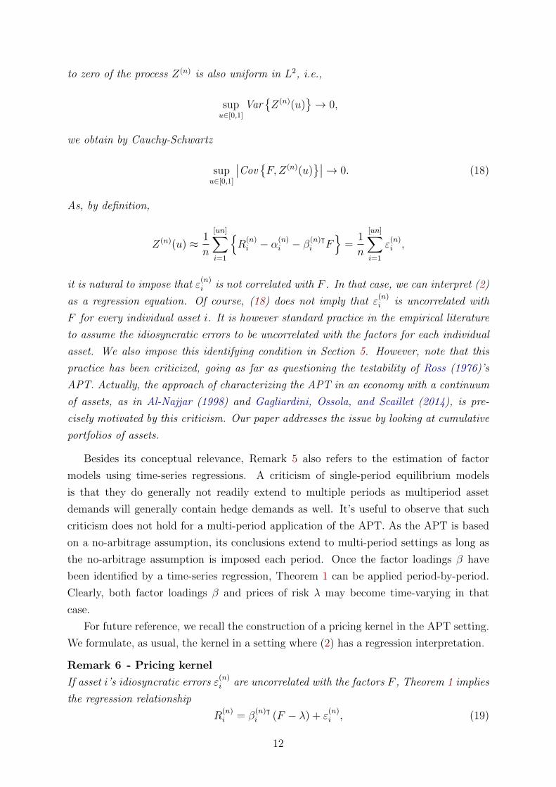
Remark 6 - Pricing kernel

If asset i’s idiosyncratic errors ε(n)i are uncorrelated with the factors F , Theorem 1 implies

the regression relationship

R(n)i = β

(n)ᵀi (F − λ) + ε

(n)i , (19)

12

with Eε(n)i = 0 and Cov

F, ε

(n)i

= 0.

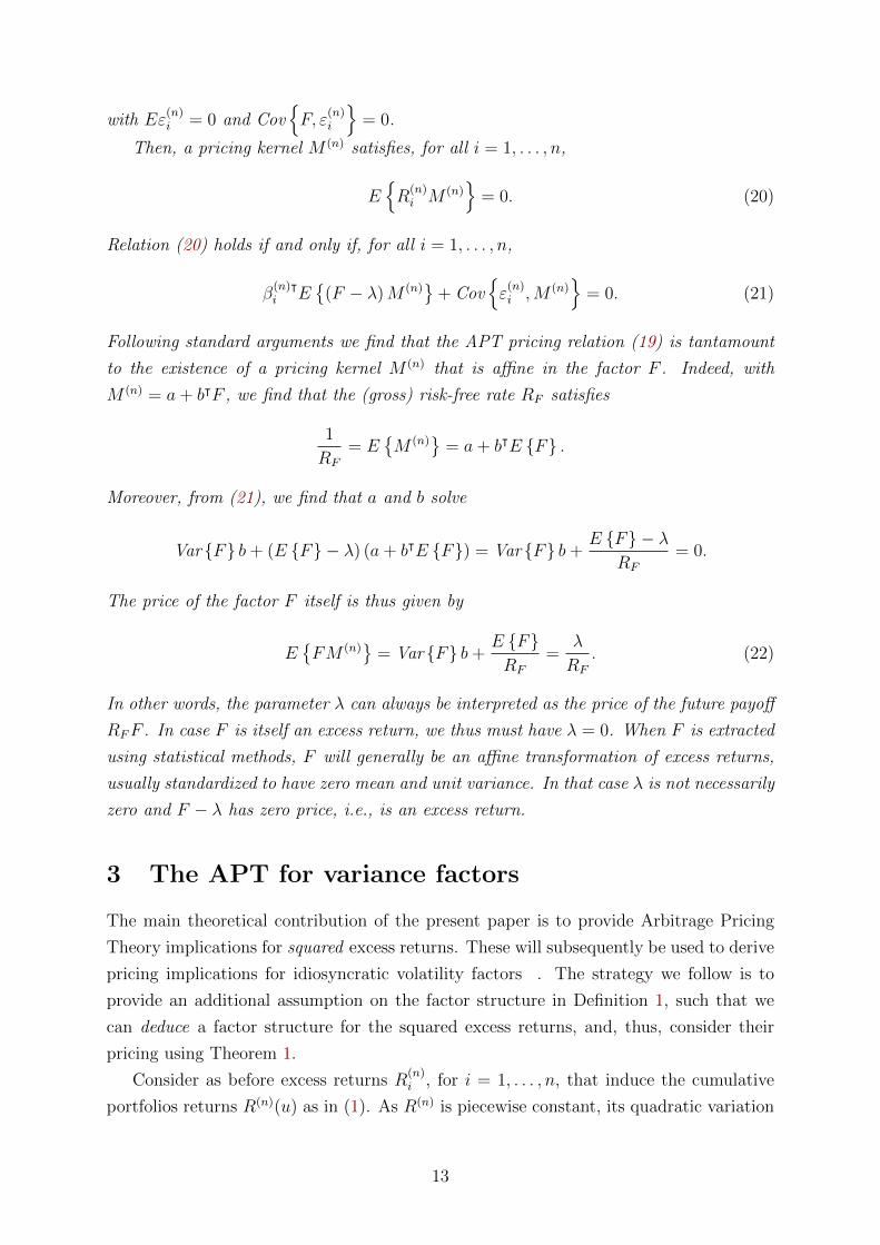
Then, a pricing kernel M (n) satisfies, for all i = 1, . . . , n,

ER

(n)i M (n)

= 0. (20)

Relation (20) holds if and only if, for all i = 1, . . . , n,

β(n)ᵀi E

(F − λ)M (n)

+ Cov

ε

(n)i ,M (n)

= 0. (21)

Following standard arguments we find that the APT pricing relation (19) is tantamount

to the existence of a pricing kernel M (n) that is affine in the factor F . Indeed, with

M (n) = a+ bᵀF , we find that the (gross) risk-free rate RF satisfies

1

RF

= EM (n)

= a+ bᵀE F .

Moreover, from (21), we find that a and b solve

Var F b+ (E F − λ) (a+ bᵀE F) = Var F b+E F − λ

RF

= 0.

The price of the factor F itself is thus given by

EFM (n)

= Var F b+

E FRF

=λ

RF

. (22)

In other words, the parameter λ can always be interpreted as the price of the future payoff

RFF . In case F is itself an excess return, we thus must have λ = 0. When F is extracted

using statistical methods, F will generally be an affine transformation of excess returns,

usually standardized to have zero mean and unit variance. In that case λ is not necessarily

zero and F − λ has zero price, i.e., is an excess return.

3 The APT for variance factors

The main theoretical contribution of the present paper is to provide Arbitrage Pricing

Theory implications for squared excess returns. These will subsequently be used to derive

pricing implications for idiosyncratic volatility factors . The strategy we follow is to

provide an additional assumption on the factor structure in Definition 1, such that we

can deduce a factor structure for the squared excess returns, and, thus, consider their

pricing using Theorem 1.

Consider as before excess returns R(n)i , for i = 1, . . . , n, that induce the cumulative

portfolios returns R(n)(u) as in (1). As R(n) is piecewise constant, its quadratic variation

13

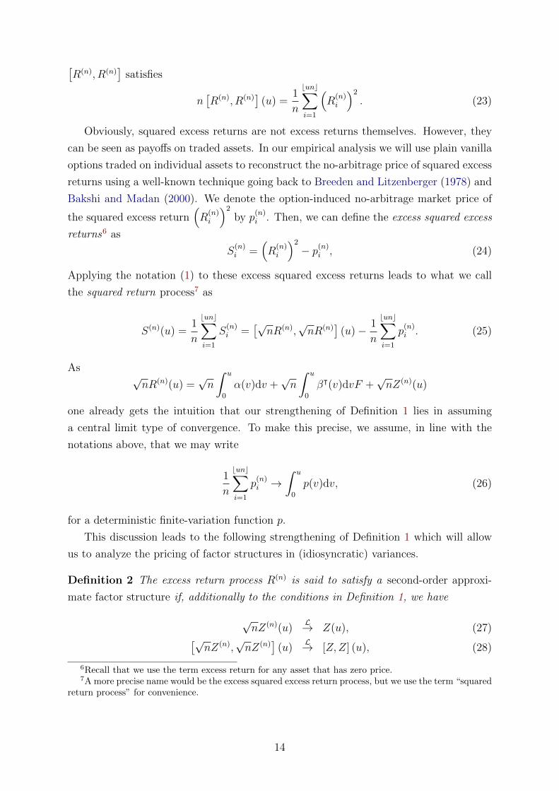
[R(n), R(n)

]satisfies

n[R(n), R(n)

](u) =

1

n

bunc∑i=1

(R

(n)i

)2

. (23)

Obviously, squared excess returns are not excess returns themselves. However, they

can be seen as payoffs on traded assets. In our empirical analysis we will use plain vanilla

options traded on individual assets to reconstruct the no-arbitrage price of squared excess

returns using a well-known technique going back to Breeden and Litzenberger (1978) and

Bakshi and Madan (2000). We denote the option-induced no-arbitrage market price of

the squared excess return(R

(n)i

)2

by p(n)i . Then, we can define the excess squared excess

returns6 as

S(n)i =

(R

(n)i

)2

− p(n)i , (24)

Applying the notation (1) to these excess squared excess returns leads to what we call

the squared return process7 as

S(n)(u) =1

n

bunc∑i=1

S(n)i =

[√nR(n),

√nR(n)

](u)− 1

n

bunc∑i=1

p(n)i . (25)

As√nR(n)(u) =

√n

∫ u

0

α(v)dv +√n

∫ u

0

βᵀ(v)dvF +√nZ(n)(u)

one already gets the intuition that our strengthening of Definition 1 lies in assuming

a central limit type of convergence. To make this precise, we assume, in line with the

notations above, that we may write

1

n

bunc∑i=1

p(n)i →

∫ u

0

p(v)dv, (26)

for a deterministic finite-variation function p.

This discussion leads to the following strengthening of Definition 1 which will allow

us to analyze the pricing of factor structures in (idiosyncratic) variances.

Definition 2 The excess return process R(n) is said to satisfy a second-order approxi-

mate factor structure if, additionally to the conditions in Definition 1, we have

√nZ(n)(u)

L→ Z(u), (27)[√nZ(n),

√nZ(n)

](u)

L→ [Z,Z] (u), (28)

6Recall that we use the term excess return for any asset that has zero price.7A more precise name would be the excess squared excess return process, but we use the term “squared

return process” for convenience.

14

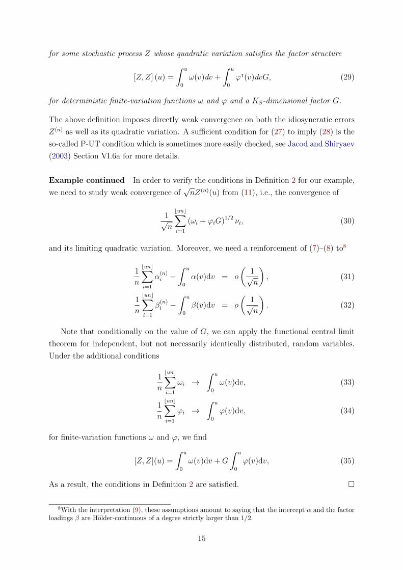
for some stochastic process Z whose quadratic variation satisfies the factor structure

[Z,Z] (u) =

∫ u

0

ω(v)dv +

∫ u

0

ϕᵀ(v)dvG, (29)

for deterministic finite-variation functions ω and ϕ and a KS-dimensional factor G.

The above definition imposes directly weak convergence on both the idiosyncratic errors

Z(n) as well as its quadratic variation. A sufficient condition for (27) to imply (28) is the

so-called P-UT condition which is sometimes more easily checked, see Jacod and Shiryaev

(2003) Section VI.6a for more details.

Example continued In order to verify the conditions in Definition 2 for our example,

we need to study weak convergence of√nZ(n)(u) from (11), i.e., the convergence of

1√n

bunc∑i=1

(ωi + ϕiG)1/2 νi, (30)

and its limiting quadratic variation. Moreover, we need a reinforcement of (7)–(8) to8

1

n

bunc∑i=1

α(n)i −

∫ u

0

α(v)dv = o

(1√n

), (31)

1

n

bunc∑i=1

β(n)i −

∫ u

0

β(v)dv = o

(1√n

). (32)

Note that conditionally on the value of G, we can apply the functional central limit

theorem for independent, but not necessarily identically distributed, random variables.

Under the additional conditions

1

n

bunc∑i=1

ωi →∫ u

0

ω(v)dv, (33)

1

n

bunc∑i=1

ϕi →∫ u

0

ϕ(v)dv, (34)

for finite-variation functions ω and ϕ, we find

[Z,Z](u) =

∫ u

0

ω(v)dv +G

∫ u

0

ϕ(v)dv, (35)

As a result, the conditions in Definition 2 are satisfied.

8With the interpretation (9), these assumptions amount to saying that the intercept α and the factorloadings β are Holder-continuous of a degree strictly larger than 1/2.

15

The main theoretical result of our paper is now the following.

Theorem 2 If the excess return process R(n) satisfies a second-order approximate factor

structure and (26) holds, then the squared return process S(n) satisfies an approximate

factor structure with α given by

αS(u) = ω(u)− p(u), (36)

factors9 vech ([F − λ] [F − λ]ᵀ), with loadings

βSF (u) = vech (β(u)βᵀ(u)) , (37)

and additional factors G with loadings

βSG(u) = ϕ(u). (38)

As the squared return process S(n) satisfies an approximate factor structure, Theorem 1

immediately gives the following corollary.

Corollary 1 If the excess return process R(n) satisfies a second-order approximate factor

structure and (26) holds, then there exists a K(K + 1)/2-dimensional vector of prices of

risk δ and a KS-dimensional vector of prices of risk η such that

ω(u)− p(u) = −vech (β(u)βᵀ(u))ᵀ δ − ϕᵀ(u)η. (39)

Corollary 1 precisely identifies the consequence of the no-arbitrage condition for the

prices of squared returns and, thereby, for the prices of common factors in (idiosyncratic)

variances. The first term in (39) gives the effect of the linear return factors F on prices of

squared returns. It’s intuitively clear that this effect exists, but the present paper seems

to be the first to make this precise. Alternatively stated, the first term in (39) also gives

the consequences for pricing “idiosyncratic” variances in case some factors have been

omitted in the linear return factor model. Clearly, in such case of omitted linear return

factors, the term “idiosyncratic” is a misnomer. This means that existing results in the

literature on common volatility factors must always be discussed relative to the linear

return factors they take into account (be it PCA or Fama-French type factors). Also

observe that the price of risk for squared (excess) returns to the squared factor loadings

vech (β(u)βᵀ(u)) are given by a parameter δ that is unrelated to the prices of risk at the

linear return factor model λ. An empirical advantage of this finding is that inference

about the price of squared returns/idiosyncratic variances is not hampered by possibly

weak identification of the price of risk λ.

9For a symmetric K × K matrix A, vech(A) equals the K(K + 1)/2 column vector obtained byvectorizing the lower triangular part of A.

16

The second term in (39), ϕᵀ(u)η, gives the pricing effect of common factors in truly

idiosyncratic variances. Quadratic returns command a linear risk premium from exposure

to the common idiosyncratic variance factor G. This risk premium is, as in the standard

APT, linear in the exposure of the individual squared return to the common idiosyncratic

variance factor, i.e., linear in ϕ. Notice that the idiosyncratic variance factor G may be

correlated with the linear return factors F or their squares. The no-arbitrage condition

does neither impose nor exclude this.

Our main theoretical result in Theorem 2 can also be written in the form of a beta-

pricing relationship for return variance, much akin the standard beta-pricing relation for

expected returns. We explain this is the setting of our example that also forms the basis

of our empirical study in Section 5.

Example continued Using Theorem 1, we again find

Ri = βᵀi (F − λ) + εi,

with

εi = (ωi + ϕiG)1/2 νi.

This immediately implies

Var Ri = βᵀi Var F βi + ωi + ϕᵀiE G .

Assume, similarly to the assumption discussed in Remark 5, that the pricing relation-

ship (39) is valid for each asset individually, i.e.,

ωi − pi = −vech (βiβᵀi )ᵀ δ − ϕᵀi η.

Then, we have for each asset,

E Ri = βᵀi E F − λ ,

Var Ri − pi = vech (βiβᵀi )ᵀ [vech (Var F)− δ] + ϕᵀiE G− η .

The first equation is the standard beta pricing relation for expected excess returns. Sim-

ilarly, the second equation gives a beta-type pricing relation for the variance of excess

returns. When seen as an expected excess return, after subtracting the price pi of

the squared return, the excess return variance displays a beta-type pricing relation with

coefficients ϕi vis-a-vis the variance factors G. Note however the correction with the

premium on the variance of the factors. The various prices of risk can also be understood

through the study of the induced pricing kernel .

17

Remark 7 - Dynamic Factor Models As mentioned before, our pricing results can

be used as well in a dynamic setting in which case the moments of interest would be

conditional on the relevant past information. While conditional beta pricing has a long

history , conditional factor models have also been used to get more parsimonious models of

conditional variances of returns . This paper is one of the first to bridge the gap between

these two strands of literature. Typically, a model like (10) provides a parsimonious model

for the conditional variance of returns. In a more general formulation, we may write the

conditional variance of excess returns as

Vart−1 (Rit)ni=1 = Ω + ΦᵀEt−1 GGᵀΦ.

where Ω and Φ are coefficient matrices describing the (joint) volatility dynamics of the

excess returns. As a result, the idiosyncratic variance factors G, besides their role in

pricing nonlinear derivatives, also provide information on the volatility dynamics that

are not already captured by the factors F at the linear excess return level.

Before turning to standard Fama and MacBeth (1973) regressions and GMM methods

to identify, in particular, the prices of risk η for the idiosyncratic variance factors, we

conclude this section with a remark concerning the price of skewness and kurtosis.

Remark 8 - Pricing skewness and kurtosis The pricing kernel M has so far been

characterized using no arbitrage conditions only. However, it is possible to come up

with economic interpretations of M based on the characterization of an equilibrium in an

economy with an exogenous supply of risky assets. It is well known that if investors only

care about the mean and the variance of returns, the only relevant pricing factor is the

excess market return, say F = RM −RF . However, if agents also care about skewness, it

is known that the squared excess market return becomes a relevant factor as well . This

would imply a pricing kernel of the form

M = a+ b (RM −RF ) + c[(RM −RF )2 − Π (RM −RF )2] ,

where Π denotes the pricing operator ΠX = E XM.Based on small noise expansions,Chabi-Yo, Leisen, and Renault (2014) have shown

that the value of b and c would be

b = − 1

RF

1

τ, c =

1

RF

ρ

τ 2,

where τ and ρ stand for an average (across investors) of risk tolerances and skewness

tolerances, respectively. However, Chabi-Yo, Leisen, and Renault (2014) also point out

that when investors have heterogeneous preferences for skewness, an additional factor G

18

should be introduced

M = a+ b (RM −RF ) + c[(RM −RF )2 − Π (RM −RF )2]+ dG.

In terms of excess return, we have

G = (RM −RF )(Rsk −RF )− Π(RmRsk) + 2RF −R2F

where Rsk is a portfolio return defined from the affine regression of R2M on the ”linear”

returns Ri, i = 1, ...n, i.e.,

Cov[R2M , (Ri)1≤i≤n

][V ar (Ri)1≤i≤n]−1 (Ri)1≤i≤n = A+BRsk.

In other words, it is precisely because the squared market return cannot be perfectly

traded with linear portfolios that an additional factor shows up, that does not coincide

with the cubic market return R3M , usually introduced to price kurtosis. Note that the

coefficient of G in the pricing kernel M is precisely non zero because skewness tolerances

are heterogeneous across investors

d =2

RF

V ar(ρ)

τ 3,

where V ar(ρ) stands for the cross-sectional variance (across investors) of skewness tol-

erances. Note that this remark does not preclude the introduction within G (and thus

also in the pricing kernel) an additional factor R3M precisely focused on pricing kurtosis.

Chabi-Yo, Leisen, and Renault (2014) show that its coefficient in the pricing kernel will

be proportional to an average kurtosis tolerance. This is in line with pricing the risk

encapsulated in squared returns, that is the variance of squared returns.

4 Data

4.1 Sample construction

Each last trading day of the month for the period between January 1996 and December

2013, we extract the index constituents of the S&P500 index from Compustat (using

ticker “I0003”). We merge the stock indentifying information with daily stock returns

from CRSP using the WRDS linking table and compute cumulative 30-calendar day

returns from month end to match the maturity of the OptionMetrics implied volatility

surface detailed below. We merge the stock data from CRSP with the OptionMetrics

standardized implied volatility surface for a maturity of 30 calendar days. The implied

volatility surface contains smoothed implied volatilities for a standardized set of deltas

19

ranging from -0.8 to -0.2 for puts and 0.2 to 0.8 for calls, as well as an implied option

premium and implied strike price for each standardized option contract. We retain only

those observations for which the implied option premium and the implied strike price are

larger than zero, and the smoothed implied volatility is finite. We compute the stock’s

forward price using realised dividends over the life of the option from the OptionMetrics

dividend file, discounted using the interpolated risk-free rates in the OptionMetrics zero-

coupon yield file.

Call and put implied volatility smiles are not always identical, and the standardized

call and put deltas yield slightly different implied strike prices, i.e., moneyness defined

as the strike price over the forward price. We obtain one implied volatility smile per

stock-date as follows. First, we interpolate the smoothed call implied volatilities at the

put option implied strike prices and vice versa to obtain call and put smoothed implied

volatilities for all observed implied strike prices. Then we average the put and call implied

volatility for each strike price. We use the vector of average smoothed implied volatilities

to compute implied volatilities for non-observed moneyness levels using linear interpola-

tion. Outside the observed range of moneyness levels, we assume the implied volatility is

constant at the endpoints in the observed data. We compute Black-Scholes option prices

from the interpolated implied volatility curve for each stock-date combination.

Following Bakshi and Madan (2000), any twice differentiable payoff function of the

stock, H(S), can be spanned as a static portfolio of plain vanilla European put (P (K))

and call (C(K)) options10, a bond and a forward contract,

H(S) = H(K0) + (S −K0)HS(K0) + erτ∫ K0

0

HSS(K)P (K)dK

+ erτ∫ ∞K0

HSS(K)C(K)dK, (40)

with K0 a predetermined cut-off level separating the strike space into put and call options,

r the continuously-compounded risk-free rate and τ the relevant maturity. We seek to

compute the price of the discretely compounded squared excess return,

pit = EQR2iT

= EQ H(S) ,

with

H(S) =

(S

S0

− erτ)2

, (41)

10Individual equity options are American rather than European. Since we use only out-of-the-moneyoptions, the early exercise premium will be small. Ofek, Richardson, and Whitelaw (2004) report amedian early exercise premium equal to 70 bps for at-the-money put options. The bid-ask spread ofthose options is an order of magnitude larger than that.

20

so that

HS(S) =2

S0

(S

S0

− erτ), (42)

HSS(S) =2

S20

. (43)

Plugging (41)-(43) into (40), setting K0 = S0 and taking risk-neutral expectations, we

obtain

pit = (1− erτ )2 +2

S0

(1− erτ ) +2

S20

∫ S0

0

P (K)dK +2

S20

∫ ∞S0

C(K)dK, (44)

which shows that for the squared excess return, each of the options in the replicating

portfolio will be given the same weight. The put price is integrable as a function of the

strike price over any interval of the form [a, b) for a ≥ 0, b < ∞ and in particular up to

the current spot price that we use as a cut-off. The call price is integrable as a function of

the strike price over any interval on the positive real axis, which ensures that the integral

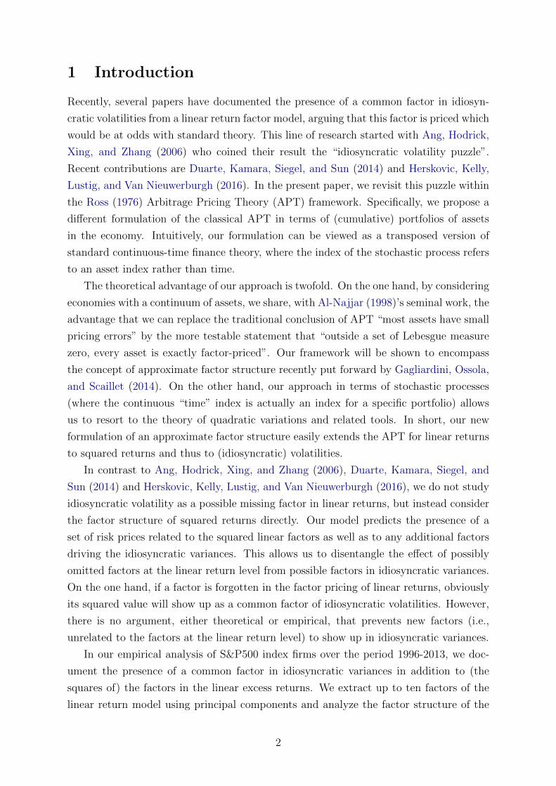
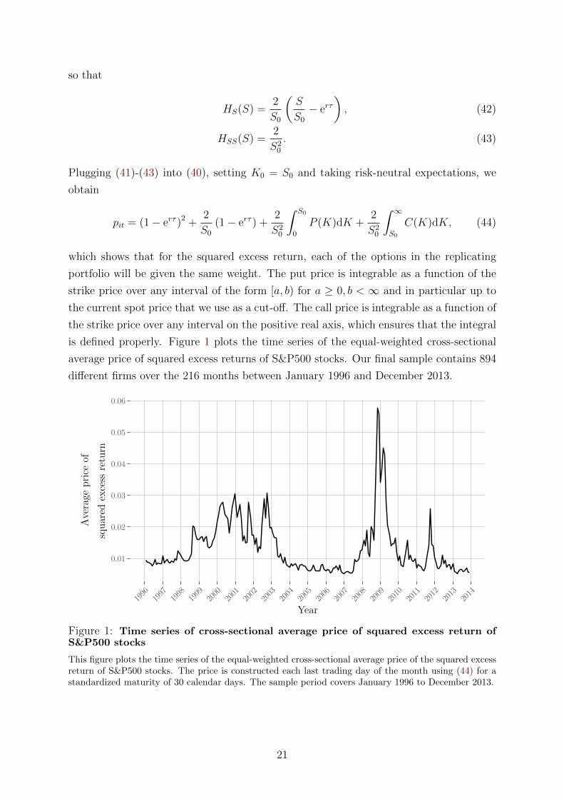
is defined properly. Figure 1 plots the time series of the equal-weighted cross-sectional

average price of squared excess returns of S&P500 stocks. Our final sample contains 894

different firms over the 216 months between January 1996 and December 2013.

0.01

0.02

0.03

0.04

0.05

0.06

1996

1997

1998

1999

2000

2001

2002

2003

2004

2005

2006

2007

2008

2009

2010

2011

2012

2013

2014

Year

Average

price

of

squared

excess

return

Figure 1: Time series of cross-sectional average price of squared excess return ofS&P500 stocks

This figure plots the time series of the equal-weighted cross-sectional average price of the squared excessreturn of S&P500 stocks. The price is constructed each last trading day of the month using (44) for astandardized maturity of 30 calendar days. The sample period covers January 1996 to December 2013.

21

5 Squared return factors in S&P500 stocks

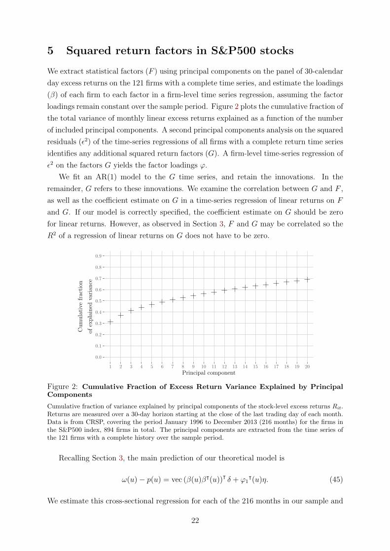
We extract statistical factors (F ) using principal components on the panel of 30-calendar

day excess returns on the 121 firms with a complete time series, and estimate the loadings

(β) of each firm to each factor in a firm-level time series regression, assuming the factor

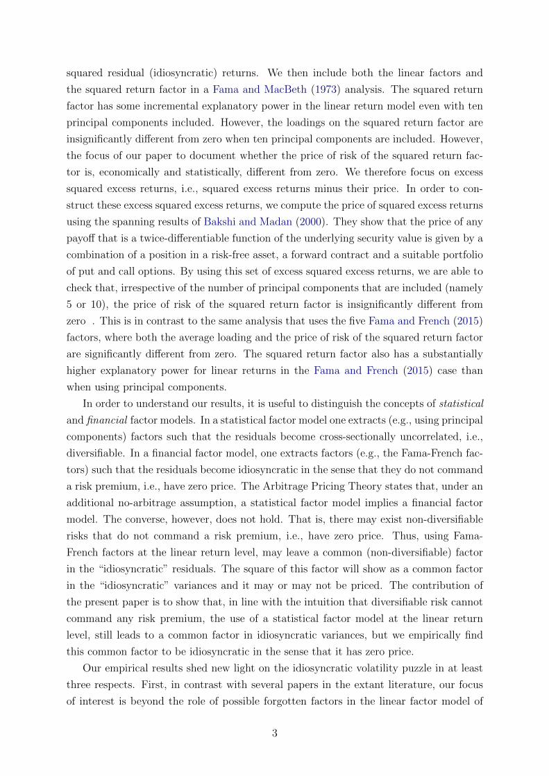
loadings remain constant over the sample period. Figure 2 plots the cumulative fraction of

the total variance of monthly linear excess returns explained as a function of the number

of included principal components. A second principal components analysis on the squared

residuals (ε2) of the time-series regressions of all firms with a complete return time series

identifies any additional squared return factors (G). A firm-level time-series regression of

ε2 on the factors G yields the factor loadings ϕ.

We fit an AR(1) model to the G time series, and retain the innovations. In the

remainder, G refers to these innovations. We examine the correlation between G and F ,

as well as the coefficient estimate on G in a time-series regression of linear returns on F

and G. If our model is correctly specified, the coefficient estimate on G should be zero

for linear returns. However, as observed in Section 3, F and G may be correlated so the

R2 of a regression of linear returns on G does not have to be zero.

0.0

0.1

0.2

0.3

0.4

0.5

0.6

0.7

0.8

0.9

1 2 3 4 5 6 7 8 9 10 11 12 13 14 15 16 17 18 19 20

Principal component

Cumulative

fraction

ofexplained

varian

ce

Figure 2: Cumulative Fraction of Excess Return Variance Explained by PrincipalComponents

Cumulative fraction of variance explained by principal components of the stock-level excess returns Rit.Returns are measured over a 30-day horizon starting at the close of the last trading day of each month.Data is from CRSP, covering the period January 1996 to December 2013 (216 months) for the firms inthe S&P500 index, 894 firms in total. The principal components are extracted from the time series ofthe 121 firms with a complete history over the sample period.

Recalling Section 3, the main prediction of our theoretical model is

ω(u)− p(u) = vec (β(u)βᵀ(u))ᵀ δ + ϕ1ᵀ(u)η. (45)

We estimate this cross-sectional regression for each of the 216 months in our sample and

22

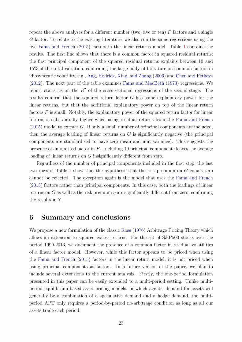
repeat the above analyses for a different number (two, five or ten) F factors and a single

G factor. To relate to the existing literature, we also run the same regressions using the

five Fama and French (2015) factors in the linear returns model. Table 1 contains the

results. The first line shows that there is a common factor in squared residual returns;

the first principal component of the squared residual returns explains between 10 and

15% of the total variation, confirming the large body of literature on common factors in

idiosyncratic volatility, e.g., Ang, Hodrick, Xing, and Zhang (2006) and Chen and Petkova

(2012). The next part of the table examines Fama and MacBeth (1973) regressions. We

report statistics on the R2 of the cross-sectional regressions of the second-stage. The

results confirm that the squared return factor G has some explanatory power for the

linear returns, but that the additional explanatory power on top of the linear return

factors F is small. Notably, the explanatory power of the squared return factor for linear

returns is substantially higher when using residual returns from the Fama and French

(2015) model to extract G. If only a small number of principal components are included,

then the average loading of linear returns on G is significantly negative (the principal

components are standardised to have zero mean and unit variance). This suggests the

presence of an omitted factor in F . Including 10 principal components leaves the average

loading of linear returns on G insignificantly different from zero.

Regardless of the number of principal components included in the first step, the last

two rows of Table 1 show that the hypothesis that the risk premium on G equals zero

cannot be rejected. The exception again is the model that uses the Fama and French

(2015) factors rather than principal components. In this case, both the loadings of linear

returns on G as well as the risk premium η are significantly different from zero, confirming

the results in ?.

6 Summary and conclusions

We propose a new formulation of the classic Ross (1976) Arbitrage Pricing Theory which

allows an extension to squared excess returns. For the set of S&P500 stocks over the

period 1999-2013, we document the presence of a common factor in residual volatilities

of a linear factor model. However, while this factor appears to be priced when using

the Fama and French (2015) factors in the linear return model, it is not priced when

using principal components as factors. In a future version of the paper, we plan to

include several extensions to the current analysis. Firstly, the one-period formulation

presented in this paper can be easily extended to a multi-period setting. Unlike multi-

period equilibrium-based asset pricing models, in which agents’ demand for assets will

generally be a combination of a speculative demand and a hedge demand, the multi-

period APT only requires a period-by-period no-arbitrage condition as long as all our

assets trade each period.

23

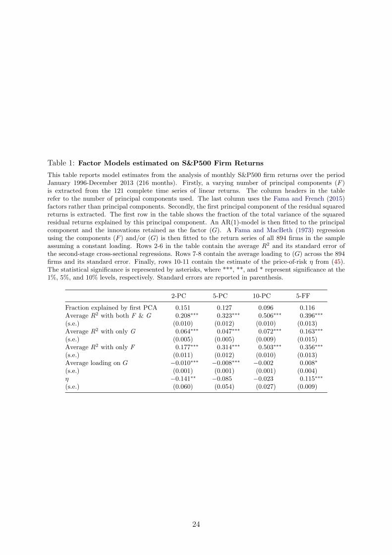
Table 1: Factor Models estimated on S&P500 Firm Returns

This table reports model estimates from the analysis of monthly S&P500 firm returns over the periodJanuary 1996-December 2013 (216 months). Firstly, a varying number of principal components (F )is extracted from the 121 complete time series of linear returns. The column headers in the tablerefer to the number of principal components used. The last column uses the Fama and French (2015)factors rather than principal components. Secondly, the first principal component of the residual squaredreturns is extracted. The first row in the table shows the fraction of the total variance of the squaredresidual returns explained by this principal component. An AR(1)-model is then fitted to the principalcomponent and the innovations retained as the factor (G). A Fama and MacBeth (1973) regressionusing the components (F ) and/or (G) is then fitted to the return series of all 894 firms in the sampleassuming a constant loading. Rows 2-6 in the table contain the average R2 and its standard error ofthe second-stage cross-sectional regressions. Rows 7-8 contain the average loading to (G) across the 894firms and its standard error. Finally, rows 10-11 contain the estimate of the price-of-risk η from (45).The statistical significance is represented by asterisks, where ***, **, and * represent significance at the1%, 5%, and 10% levels, respectively. Standard errors are reported in parenthesis.

2-PC 5-PC 10-PC 5-FF

Fraction explained by first PCA 0.151 0.127 0.096 0.116Average R2 with both F & G 0.208∗∗∗ 0.323∗∗∗ 0.506∗∗∗ 0.396∗∗∗

(s.e.) (0.010) (0.012) (0.010) (0.013)Average R2 with only G 0.064∗∗∗ 0.047∗∗∗ 0.072∗∗∗ 0.163∗∗∗

(s.e.) (0.005) (0.005) (0.009) (0.015)Average R2 with only F 0.177∗∗∗ 0.314∗∗∗ 0.503∗∗∗ 0.356∗∗∗

(s.e.) (0.011) (0.012) (0.010) (0.013)Average loading on G −0.010∗∗∗ −0.008∗∗∗ −0.002 0.008∗

(s.e.) (0.001) (0.001) (0.001) (0.004)η −0.141∗∗ −0.085 −0.023 0.115∗∗∗

(s.e.) (0.060) (0.054) (0.027) (0.009)

24

Secondly, the pricing kernel in our model for squared returns will be quadratic in the

linear factors F and linear in the quadratic factors G. One of the criticisms of standard

(linear) factor models is that the linear version of the pricing kernel can take on negative

values. A linear-quadratic formulation opens up the possibility that the pricing kernel

will always be positive, but it is an empirical question whether that indeed is true.

A Proofs

Proof: of Theorem 1 The proof is classical, but we provide a version that is convenient

for our setup. Let h denote any portfolio without exposure to the factors, i.e., with∫ 1

u=0h(u)β(u)du = 0. Then, from (2), the induced portfolio returns are∫ 1

u=0

h(u)dR(n)(u) =

∫ 1

u=0

h(u)α(u)du+

∫ 1

u=0

h(u)dZ(n)(u). (46)

As both h and Z(n) are of finite variation, we find by partial integration∫ 1

u=0

h(u)dZ(n)(u) = Z(n)(1)h(1)−∫ 1

u=0

Z(n)(u)dh(u)−∑

0≤u≤1

∆Z(n)(u)∆h(u),

which converges to zero since Z(n) does. Consequently,∫ 1

u=0

h(u)dR(n)(u)→∫ 1

u=0

h(u)α(u)du. (47)

In the absence of arbitrage, we must have∫ 1

u=0h(u)α(u)du = 0. As this must hold for any

finite-variation function h orthogonal to all components of β, we have α(u) = −β(u)ᵀλ

for some vector λ.

Proof: of Theorem 2 As the return process R(n) satisfies the conditions of Theorem 1,

we may rewrite (1) as

R(n)i = n

[R(n)

(i

n

)−R(n)

(i− 1

n

)](48)

= n

∫ i/n

(i−1)/n

βᵀ(v)dv (F − λ) + n

[Z(n)

(i

n

)− Z(n)

(i− 1

n

)].

25

This implies

S(n)(u) =1

n

bunc∑i=1

(R

(n)i

)2

− p(n)i

= n

bunc∑i=1

[∫ i/n

(i−1)/n

βᵀ(v)dv (F − λ)

]2

− 1

n

bunc∑i=1

p(n)i (49)

+ n

bunc∑i=1

[Z(n)

(i

n

)− Z(n)

(i− 1

n

)]2

+ 2n

bunc∑i=1

∫ i/n

(i−1)/n

βᵀ(v)dv [F − λ]

[Z(n)

(i

n

)− Z(n)

(i− 1

n

)].

We consider the convergence of the above four terms separately. For simplicity, we only

give the proof for K = 1. With respect to the first term, we know that β is bounded, say

by M . We establish that this first term essentially is a Riemann sum. Indeed, we have∣∣∣∣∣∣nbunc∑i=1

(∫ i/n

(i−1)/n

β(v)dv

)2

−bunc∑i=1

β2

(i− 1

n

)1

n

∣∣∣∣∣∣=

∣∣∣∣∣∣ 1nbunc∑i=1

(n∫ i/n

(i−1)/n

β(v)dv

)2

− β2

(i− 1

n

)∣∣∣∣∣∣≤ 2M

n

bunc∑i=1

∣∣∣∣∣n∫ i/n

(i−1)/n

β(v)dv − β(i− 1

n

)∣∣∣∣∣≤ 2M

bunc∑i=1

∫ i/n

(i−1)/n

∣∣∣∣β(v)− β(i− 1

n

)∣∣∣∣ dvAs β is of bounded variation, we may write β = β+ − β− where both β+ and β− are

increasing. We thus find∣∣∣∣∣∣nbunc∑i=1

(∫ i/n

(i−1)/n

β(v)dv

)2

−bunc∑i=1

β2

(i− 1

n

)1

n

∣∣∣∣∣∣≤ 2M

bunc∑i=1

∫ i/n

(i−1)/n

∣∣∣∣β+(v)− β+

(i− 1

n

)−β−(v)− β−

(i− 1

n

)∣∣∣∣ dv≤ 2M

bunc∑i=1

∫ i/n

(i−1)/n

∣∣∣∣β+

(i

n

)− β+

(i− 1

n

)∣∣∣∣ dv +

bunc∑i=1

∫ i/n

(i−1)/n

∣∣∣∣β−( in)− β−

(i− 1

n

)∣∣∣∣ dv

≤ 2M

n[β+(1)− β+(0) + β−(1)− β−(0)] ,

which converges to zero. Consequently, the first term in (49) converges to the limit of

26

the Riemann sums∑bunc

i=1

(β(i−1n

)(F − λ)

)2 1n, i.e., to

∫ uv=0

(β(v) (F − λ))2 dv.

The second term in (49) converges given (26) and the third one in view of (28).

Finally, consider the last term in (49). By Cauchy-Schwarz and the previous results,

we find

n

bunc∑i=1

∫ i/n

(i−1)/n

[β(v)− β

(i− 1

n

)dv

] [Z(n)

(i

n

)− Z(n)

(i− 1

n

)]

≤

√√√√n

bunc∑i=1

(∫ i/n

(i−1)/n

β(v)− β(i− 1

n

)dv

)2

×

√√√√n

bunc∑i=1

[Z(n)

(i

n

)− Z(n)

(i− 1

n

)]2

For increasing β, we may bound the first square-root further by√√√√n

bunc∑i=1

(∫ i/n

(i−1)/n

β

(i

n

)− β

(i− 1

n

)dv

)2

≤

√√√√ 1

n

bunc∑i=1

(β

(i

n

)− β

(i− 1

n

))2

,

which converges to zero. For general finite-variation β the same result again follows from

writing it as the difference of two increasing functions. Consequently, the limit of the

fourth term in (49) equals that of

[F − λ]

bunc∑i=1

β

(i− 1

n

)[Z(n)

(i

n

)− Z(n)

(i− 1

n

)](50)

As√nZ(n) converges in law, the above expression converges to zero.

Taking these claims together, we find that

S(n)(u)−∫ u

v=0

(β(v) (F − λ))2 dv +

∫ u

0

p(v)dv − [Z,Z] (u), (51)

converges to zero. In view of (29), this concludes the proof.

References

Ait-Sahalia, Y., and D. Xiu (2015): “Using Principal Component Analy-

sis to Estimate a High Dimensional Factor Model with High-Frequency Data,”

http://ssrn.com/abstract=2669506.

27

Al-Najjar, N. I. (1998): “Factor Analysis and Arbitrage Pricing in Larget Asset

Economies,” Journal of Economic Theory, 78, 231–262.

(1999): “On the Robustness of Factor Structures to Asset Repackaging,” Journal

of Mathematical Economics, 31, 309–320.

Ang, A., R. J. Hodrick, Y. Xing, and X. Zhang (2006): “The Cross-Section of

Volatility,” Journal of Finance, 61(1), 259–299.

Bakshi, G., and D. Madan (2000): “Spanning and derivative-security valuation,”

Journal of Financial Economics, 55(2), 205–238.

Breeden, D., and R. Litzenberger (1978): “Prices of State-Contingent Claims

Implicit in Option Prices,” Journal of Business, 51, 621–651.

Chabi-Yo, F., D. P. Leisen, and E. Renault (2014): “Aggregation of preferences

for skewed asset returns,” Journal of Economic Theory, 154, 453–489.

Chen, Z., and R. Petkova (2012): “Does Idiosyncratic Volatility Proxy for Risk

Exposure?,” Review of Financial Studies, 25(9), 2745–2787.

Christoffersen, P., M. Fournier, and K. Jacobs (2015): “The Factor Structure

in Equity Options,” .

Duarte, J., A. Kamara, S. Siegel, and C. Sun (2014): “The systematic risk of

idiosyncratic volatility,” University of Washington working paper.

Fama, E. F., and K. R. French (2015): “A five-factor asset pricing model,” Journal

of Financial Economics, 116(1), 1–22.

Fama, E. F., and J. D. MacBeth (1973): “Risk, Return, and Equilibrium: Empirical

Tests,” Journal of Political Economy, 81(3), 607–636.

Gagliardini, P., E. Ossola, and O. Scaillet (2014): “Time-Varying Risk Premi-

ums in Large Cross-Sectional Equity Datasets,” Working Paper.

Harvey, C. R., and A. Siddique (2000): “Conditional Skewness in Asset Pricing

Tests,” The Journal of Finance, 55(3), 1263–1295.

Herskovic, B., B. Kelly, H. Lustig, and S. Van Nieuwerburgh (2016): “The

Common Factor in Idiosyncratic volatility: quantitative asset pricing implications,”

Journal of Financial Economics, 119(2), 249–283.

Jacod, J., and A. N. Shiryaev (2003): Limit Theorems for Stochastic Processes, vol.

288 of Grundlehren der mathematischen Wissenschaften. Springer Berlin Heidelberg,

Berlin, Heidelberg.

28

Kraus, A., and R. H. Litzenberger (1976): “Skewness Preference and the Valuation

of Risk Assets,” The Journal of Finance, 31(4), 1085–1100.

Mykland, P. A., and L. Zhang (2006): “ANOVA for diffusions and Ito processes,”

The Annals of Statistics, 48(34), 1931–1963.

Ofek, E., M. Richardson, and R. F. Whitelaw (2004): “Limited arbitrage and

short sales restrictions: evidence from the options markets,” Journal of Financial Eco-

nomics, 74, 305–342.

Ross, S. A. (1976): “The arbitrage theory of capital asset pricing,” Journal of Economic

Theory, 13(3), 341–360.

29