Embed Size (px)
Citation preview

Centre for the Study of Globalisation and Regionalisation (CSGR), University of Warwick, CoventryCV4 7AL, United-Kingdom. URL: http://www.csgr.org
"Pricing in Segmented Markets, Arbitrage andthe Law of One Price: Evidence from the
European Car Market"
Matthias Lutz
CSGR Working Paper No. 53/00
May 2000
Pricing in Segmented Markets, Arbitrage Barriers and the Law of One Price:Evidence from the European Car MarketMatthias Lutz1
Institute of Economics, University of St. Gallen.CSGR Working Paper No. 53/00May 2000
Abstract:
The paper examines automobile price differences in the Single Market for the 1993-98
period. The absolute law of one price is strongly rejected, but there is some convergence to its
relative version. Two sets of explanations are considered: (i) price-setting in segmented markets
and (ii) arbitrage barriers. The role of price-setting variables is seriously overestimated when
arbitrage factors are not controlled for. Evidence for Belgium and Luxembourg suggests that the
single currency will lower price differences significantly. Arbitrage trade is also likely to become
more effective if the block exemption is not extended beyond 2002.
Keywords: Law of One Price, Market Segmentation, Arbitrage, Gravity Model.
JEL classification: F14, F15, L62.
Address for correspondence:
Matthias G. LutzUniversity of St. GallenInstitute of EconomicsUniversity of St. Gallen,Dufourstrasse 48, 9000 St. Gallen, Switzerland,Tel: +41 71 224 2303Fax: +41 71 224 2646Email: [email protected]
1 The author wishes to thank above all Manfred Gärtner and Friederike Pohlenz for numerous suggestions on at least two earlierversions of this paper. Thanks also to Elisabeth Allgöwer, Rabindra Chakraborty, Marcel Savioz and Bernd Hayo, who all readthrough an earlier draft, and seminar participants at the University of St. Gallen, especially Michael Lechner, and at the 1998Annual Conference of the Verein für Socialpolitik in Rostock.

Non-Technical Summary
Car prices in the European Union vary substantially across national markets. For instance, an
identical Ford Mondeo was 40% more expensive in France than in Spain in May 1998, and 38%
more expensive in the UK than in Portugal in November 1997. Translated into absolute terms,
these figures imply that there are substantial arbitrage gains that are not exploited. Consequently,
there must be serious doubts about the validity of the law of one price and the success of the
Single Market project.
This paper presents a systematic empirical analysis of the persistent deviations from the law of
one price in the European car market during the 1993-98 period. It is based on price data for over
90 different cars across 12 national markets.
Two main explanations are examined. The first concerns the respective roles of cost and mark-up
factors under the assumption that national markets are completely segmented. The following
factors are systematically related to car price differentials: differences in tax rates,
competitiveness, market share, home market bias, and non-tariff barriers on imports from Japan.
There is also evidence that exchange rate changes are only partially passed on to prices, even
after allowing for domestic cost factors. On the cost side, differences in labour and transport
costs matter, as does the scale of a manufacturer’s operations.
The second explanation deals explicitly with barriers to arbitrage. There is a growing literature
that suggests that transaction costs are important for trade. Search costs in international trade
lead to ‘trading networks’ which serve to match international sellers and buyers, particularly in
the case of differentiated products. Such networks will develop most easily when costs are low.
The results show that absolute price differentials are systematically smaller when countries are
close to each other, share a common language or border and the lower are official trade barriers.
Arbitrage barriers also appear to be greater when the countries involved differ in the location of
the steering wheel (i.e. left-hand drive versus right-hand drive). The largest single effect comes
from sharing the same currency, as is the case in Belgium and Luxembourg. Price differentials
between these two countries are nearly four percentage points lower, even after allowing for all
other factors.
Finally, when both types of explanations are considered jointly, most variables remain
significant. However, the mark-up and cost factors matter less now. This suggests that despite
the importance of arbitrage barriers, markets are not completely segmented. When explaining the
overall dispersion of car prices across the EU, distance across markets is the single most
important explanatory factor.
How indicative is this study of a more general lack of integration in the EU? Recent surveys
show that price differences for cars are actually smaller than for many other goods. This suggests
that markets for other goods are even further from resembling a Single Market.
Two essentially political decisions are likely to influence the future of price differentiation in the
European car market.
The first is the European Commission policy towards the car industry. The current block
exemption enables manufacturers to obstruct arbitrage trade, as the Volkswagen case
demonstrates. There are few welfare grounds for extending the exemption beyond 2002, but the
manufacturers are likely to lobby hard to persuade the European Commission to do just that.
The second is the single European currency. If the Belgium-Luxembourg example is a valid
guide to its likely impact, then the single currency will help reduce price differentials in the
medium to long run.

1
1. Introduction
How is it possible that an identical Ford Mondeo was 40% more expensive in France than in Spain
in May 1998 and 38% more expensive in the UK than in Portugal in November 1997? Such price
differentials raise serious doubts about the validity of the law of one price (LOP), and should
certainly not be observed in an integrated market. This paper aims to highlight the factors that might
be responsible for such phenomena, thus adding to the empirical literature on purchasing power
parity (PPP). The final verdict on the long-run validity of PPP is still open. There are a number of
recent studies which provide support, in some cases even for LOP, but there are also dissenting
findings1. Whatever the views on PPP in the long run, there is widespread agreement that short-run
deviations are highly persistent (Rogoff, 1996). In this paper, two explanations are offered for the
persistent deviations from the law of one price in the European car market: a) price-setting in
imperfectly competitive markets and b) barriers to arbitrage.
The key aspect distinguishing this study from the general PPP literature is the use of a large data set
on the prices of individual traded goods. This has several advantages over aggregate data. First, the
absolute version of the law of one price can be tested. Second, potential biases due to index weights,
varying base periods and non-traded goods do not distort the analysis. Third, the identical goods
assumption can be examined and the price data adjusted accordingly. Fourth, price differences have
a direct interpretation and allow attaching a $ value to potential arbitrage gains. Fifth, the effect of
arbitrage barriers on price differences can be assessed directly.
There has been a small but growing number of empirical studies choosing a similar approach.
However, some have been based on disaggregated but still composite indices (e.g. Engel, 1993;
Engel and Rogers, 1996; Jenkins, 1997) and thus not been able to test LOP/PPP directly. Others
cover products of limited tradability, such as Big Macs (Cumby, 1996; Ong, 1997). In other cases,
the gains from arbitrage are probably too small for such trade to be feasible, such as The Economist
(Ghosh and Wolf, 1994; Knetter, 1997), IKEA furniture (Haskell and Wolf, 1999) or basic food
items (Froot et al., 1995). The advantage of the current study is that it covers a good that is
unambiguously tradable (automobiles), in a market that is formally integrated (the Single Market),
and where potential arbitrage gains appear to be substantial (in some cases exceeding US $5000 per
car).
1 Studies broadly supportive of PPP include Frankel and Rose (1996), Lothian and Taylor (1996), Panos et. al. (1997),Obstfeld and Taylor (1997), Campa and Wolf (1997) and Edison et. al. (1997), while Engel (1996) and O’Connell(1998) reject PPP. Froot et al. (1995) provide evidence supportive of LOP in data spanning several centuries. Surveys ofthe PPP literature can be found in Dornbusch (1988), Froot and Rogoff (1995) and Rogoff (1996).

2
Also somewhat related is the empirical Industrial Organisation (IO) literature on the European car
market, such as Mertens and Ginsburgh (1985), Kirman and Schueller (1990), Verboven (1996) and
Goldberg and Verboven (1998). The major difference is that, in contrast to the IO studies,
segmentation of national markets is not taken as given here. Instead, a major focus of the analysis is
precisely on factors that may help explain the degree of segmentation between markets. In other
words, while the IO oriented literature examines the nature of competition between similar goods
within markets, our main interest is on competition between identical goods across markets. As the
data set falls into the single market period, full market integration is, at least theoretically, a
plausible null hypothesis which can be tested. Given these different objectives, there is no explicit
modelling here of some of the structural characteristics of national car markets in Europe; readers
interested in these issues should consult the above-mentioned studies. First and foremost, this paper
fits into the tradition of empirical work on PPP and LOP.2
A possible drawback to the use of industry-specific data is that it cannot automatically be
generalised to other sectors. The European car sector has always been the target of specific forms of
intervention (Holmes and Smith, 1995). The key interference today is the sector’s block exemption
from certain aspects of European Union (EU) competition law, first granted in 1985 and now in its
second phase (1995-2002). Its key feature is that it allows manufacturers to maintain exclusive
dealership systems in each country, giving them a great deal of control over the sale of their cars.
Although explicitly outlawed by the European Commission (EC), the Volkswagen case3
demonstrates that car makers are prepared to use these powers to obstruct arbitrage between
national markets.
Is cross-border trade in the car sector more restricted than for other goods because of this? Not if
one considers some recent evidence on price differences for other goods. On the contrary, there is
evidence that price differences for cars are smaller than for many other goods. A 1998 Lehman
Brothers report (ACEA, 1999), for instance, found that the standard deviations of prices across the
Euro-11 countries were much higher for such traded goods as footwear, computers, and
pharmaceuticals. A comparison of prices carried out by the Belgian consumer organisation Test
Achats in June 1998 (BEUC, 1998) also revealed substantial differentials, e.g. 74% for a watch
(Swatch ‘The Classics’), 33% for a pair of jeans (‘Levi’s 501’), 73% for a camera (‘Canon Prima
Super 135’) and 60% for a CD (‘Andrea Bocelli’). Whatever the precise reasons, these findings
2 The most closely related study of the EU car market is Gual (1993) who also analyses competition across markets.3 The Volkswagen Group was fined ECU 102 bn in January 1998 for illegally preventing non-residents frompurchasing its cars in Italy (see Lutz, 2000, for details). Mercedes, Renault, Opel and, again, Volkswagen, are currentlyunder investigation for similar reasons.

3
suggest that markets for other goods are also far from integrated in the EU. There is thus no reason
to believe that the car market is atypical. Bearing in mind that it is the largest manufacturing sector
in Europe and that cars are the biggest single traded item in the average household consumption
basket, there is a good case for using it to learn about the limits of European integration.
Interestingly, the large projected welfare gains from the Single Market were not due to the final
removal of official trade barriers, but hinged largely on the equalisation of prices (Smith and
Venables, 1988).
The analysis proceeds as follows. Section 2 gives an overview of the data. It examines the identical
goods assumption, the distinction between ‘average’ PPP and ‘individual’ level LOP, and shows
that there are large potential arbitrage gains across the EU. Tests for absolute versus relative
LOP/PPP reveal that the absolute versions are clearly rejected. Large price differentials persist in
equilibrium, but the speed of convergence is considerably faster for individual than for average
prices. The econometric analysis trying to explain these results can be found in sections 3 and 4.
They systematically analyse the two main explanations: price-setting in segmented markets and
barriers to arbitrage. Their explanatory power is first examined in isolation, before the possible
interrelationship between the two sets of variables is considered. Section 5 discusses some
limitations of the analysis and the likely future development of the observed price differences.
Section 6 completes the paper with a set of conclusions.
2. A first look at the data
a) The data
The analysis uses pre-tax list prices for popular cars which have been published by the European
Commission (EC) on a biannual basis since 1993. The analysis covers the 1993-98 period and
includes twelve national markets: Austria, Belgium, France, Germany, Ireland, Italy, Luxembourg,
Netherlands, Portugal, Spain, Sweden and UK. A more detailed description of the data set can be
found in the Appendix. Pre-tax prices are used rather than post-tax prices since taxes are charged in
the country where the car is registered rather than where it is purchased. So from the point of view
of a potential EU buyer pre-tax prices are the relevant ones. The EC reports also contain
information whether a number of important extras (such as power steering or air-conditioning) are
included in the list prices. Additional data on the general specification of each model (engine size,
maximum speed etc.) comes from various issues of What Car? (a UK car monthly) and Auto’93-
Auto’99 (the annual car guide of the German motoring organisation ADAC).

4
For the law of one price to make sense, international price comparisons must refer to goods which
are (i) tradable and (ii) perfect substitutes. The first condition is satisfied here, since the goods in
question are generally sold in all markets4. The second condition is less easily satisfied. Although
the EC price data have been adjusted to account for differences in those equipment items not
explicitly mentioned in the reports, some variations remain across markets. These are either due to
the specification aspects explicitly covered in the EC reports, or when the model comes with a
different body shape or engine in a specific country.
b) Controlling for equipment differences
To obtain prices that refer to identical models, a hedonic price function was estimated. Hedonic
price functions model variations in the prices of differentiated products as a function of variations in
their characteristics. The estimated coefficients (sometimes referred to as implicit prices) can then
be used to attach a weight to each characteristic in the final price. Following standard practice in the
literature, the hedonic price function is assumed to take the form
24 12 12
1 1 1
ln itj m tj itjm t j
P a b e= = =
= + + +∑ ∑∑itjX z (1)
where Pitj is the final price and Xitj a row vector consisting of the physical characteristics of model i
at time t in country j, z a column vector of implicit prices and eitj a stochastic error term. The am and
btj terms are included to capture manufacturer and time-and-country specific effects, respectively.
Equation (1) was estimated by ordinary least squares (OLS) including 19 different characteristics5.
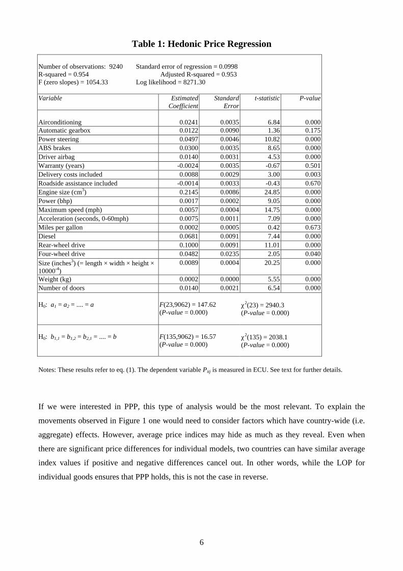
The results are shown in Table 1. The regression model fits the data very well, explaining more than
95% of the variation in prices across models and markets. All the statistically significant
coefficients have the expected sign. The time-and-country and manufacturer-specific effects are
highly significant.
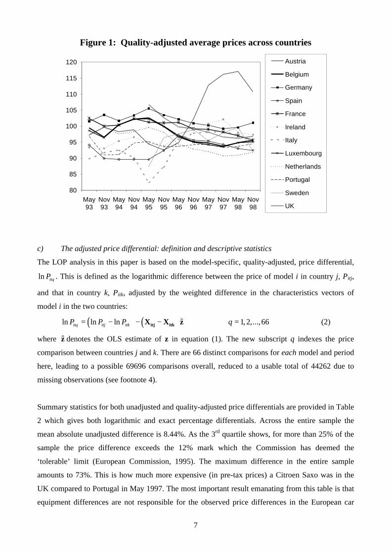
The estimated tjb terms can be used to form quality-adjusted PPP (i.e. unweighted average price)
indices for each country and time period. These are shown in Figure 1 (using Belgium in September
1995 as the base). There is considerable variation, not only between countries at each point in time,
but also with respect to the relative ranking of individual countries over time. The most extreme
cases are Italy, Sweden and the UK, three countries that experienced sizable fluctuations in their
4 There are cases where data is not available, which can be for a number of reasons. A model may no longer feature inthe EC Reports if production ceases (e.g. the Rover 111 after 1995), or new models appear only in later reports (e.g. theAudi A3 from 1997). Certain models or makes are not sold in a given market (e.g. Lancia after it withdrew from the UKand Irish markets in 1994). Sometimes data for a given model is missing from a particular edition. Also, Austria andSweden do not feature in the 1993-94 reports, having officially joined the EU in 1995. These data limitations reduce thesample to 9240 observations (from a a possible total of 11986).5 All estimation was performed with T.S.P. 4.4.

5
exchange rates. In 1995, for instance, Italy was the cheapest market on average, but in November
1997 it had become the fourth most expensive. Sweden was the second cheapest market in May
1995, became the second most expensive in May 1998, only to turn into the second cheapest again
in November 1998. The UK was the third cheapest market on average in November 1995, but
became the most expensive 12 months later and remained so until the end of the sample period.
6
Table 1: Hedonic Price Regression
Number of observations: 9240 Standard error of regression = 0.0998R-squared = 0.954 Adjusted R-squared = 0.953F (zero slopes) = 1054.33 Log likelihood = 8271.30
Variable EstimatedCoefficient
StandardError
t-statistic P-value
Airconditioning 0.0241 0.0035 6.84 0.000Automatic gearbox 0.0122 0.0090 1.36 0.175Power steering 0.0497 0.0046 10.82 0.000ABS brakes 0.0300 0.0035 8.65 0.000Driver airbag 0.0140 0.0031 4.53 0.000Warranty (years) -0.0024 0.0035 -0.67 0.501Delivery costs included 0.0088 0.0029 3.00 0.003Roadside assistance included -0.0014 0.0033 -0.43 0.670Engine size (cm3) 0.2145 0.0086 24.85 0.000Power (bhp) 0.0017 0.0002 9.05 0.000Maximum speed (mph) 0.0057 0.0004 14.75 0.000Acceleration (seconds, 0-60mph) 0.0075 0.0011 7.09 0.000Miles per gallon 0.0002 0.0005 0.42 0.673Diesel 0.0681 0.0091 7.44 0.000Rear-wheel drive 0.1000 0.0091 11.01 0.000Four-wheel drive 0.0482 0.0235 2.05 0.040Size (inches3) (= length × width × height ×10000-4)
0.0089 0.0004 20.25 0.000
Weight (kg) 0.0002 0.0000 5.55 0.000Number of doors 0.0140 0.0021 6.54 0.000
H0: a1 = a2 = .... = a F(23,9062) = 147.62(P-value = 0.000)
χ2(23) = 2940.3(P-value = 0.000)
H0: b1,1 = b1,2 = b2,1 = .... = b F(135,9062) = 16.57(P-value = 0.000)
χ2(135) = 2038.1(P-value = 0.000)
Notes: These results refer to eq. (1). The dependent variable Pitj is measured in ECU. See text for further details.
If we were interested in PPP, this type of analysis would be the most relevant. To explain the
movements observed in Figure 1 one would need to consider factors which have country-wide (i.e.
aggregate) effects. However, average price indices may hide as much as they reveal. Even when
there are significant price differences for individual models, two countries can have similar average
index values if positive and negative differences cancel out. In other words, while the LOP for
individual goods ensures that PPP holds, this is not the case in reverse.
7
Figure 1: Quality-adjusted average prices across countries
80
85
90
95
100
105
110
115
120
May93
Nov93
May94
Nov94
May95
Nov95
May96
Nov96
May97
Nov97
May98
Nov98
Austria
Belgium
Germany
Spain
France
Ireland
Italy
Luxembourg
Netherlands
Portugal
Sweden
UK
c) The adjusted price differential: definition and descriptive statistics
The LOP analysis in this paper is based on the model-specific, quality-adjusted, price differential,
ln itqP . This is defined as the logarithmic difference between the price of model i in country j, Pitj,
and that in country k, Pitk, adjusted by the weighted difference in the characteristics vectors of
model i in the two countries:
( ) ( ) ˆln ln ln 1, 2,...,66itq itj itkP P P q= − − − =itj itkX X z (2)
where z denotes the OLS estimate of z in equation (1). The new subscript q indexes the price
comparison between countries j and k. There are 66 distinct comparisons for each model and period
here, leading to a possible 69696 comparisons overall, reduced to a usable total of 44262 due to
missing observations (see footnote 4).
Summary statistics for both unadjusted and quality-adjusted price differentials are provided in Table
2 which gives both logarithmic and exact percentage differentials. Across the entire sample the
mean absolute unadjusted difference is 8.44%. As the 3rd quartile shows, for more than 25% of the
sample the price difference exceeds the 12% mark which the Commission has deemed the
‘tolerable’ limit (European Commission, 1995). The maximum difference in the entire sample
amounts to 73%. This is how much more expensive (in pre-tax prices) a Citroen Saxo was in the
UK compared to Portugal in May 1997. The most important result emanating from this table is that
equipment differences are not responsible for the observed price differences in the European car

8
market. In fact, adjusted price differentials tend to be slightly larger than unadjusted ones. This
suggests that, on average, manufacturers have not fully passed on the costs of these characteristics.
Whatever the precise reason, the differences between adjusted and unadjusted price differentials are
small.
Table 2: Summary Statistics for Price Differentials
Logarithmic Differentials Percentage Differentials
Unadjusted(1)
Adjusted(2)
Unadjusted(3)
Adjusted(4)
Number of Obs. 44262 44262 44262 44262
Mean 0.081 0.084 8.44 8.73
1st Quartile 0.029 0.030 2.91 3.01
Median 0.065 0.067 6.73 6.95
3rd Quartile 0.116 0.120 12.35 12.75
Maximum 0.549 0.554 73.14 73.97
Notes: The logarithmic adjusted price differential is calculated as in eq. (2). The exact percentage differential is based
on its antilog, e.g. in the case of column (2) as ( ){ }( )exp ln 1 *100itqabs P − .
Figures 2 and 3 give a visual impression of the variations in adjusted price differentials over time
and across manufacturers. Despite the removal of the last trade barriers at the beginning of 1993,
there is no downward trend in price differentials. The mean absolute percentage difference in the
last period at 8.11% was only marginally lower than the 8.25% in the first period. There is more
variation across manufacturers, as Figure 3 demonstrates. Here the mean for Subaru at 11.61% was
nearly twice that for Mercedes-Benz at 6.21%. While price differentials tend to be smallest for the
luxury car makers, such as Mercedes, Audi, BMW and Volvo, there is little evidence that Japanese
manufacturers price-discriminate more than other manufacturers. Honda, Toyota, Mitsubishi and
Mazda are found in the lower half, Nissan, Daihatsu, Suzuki and Subaru in the upper half of the
ranking. Do larger manufacturers differentiate less between markets? Again, there is no clear
evidence either way: of the six major manufacturers, Renault, VW and Opel/Vauxhall are found in
the lower, Peugeot, Fiat and Ford in the upper half.

9
So far only relative price differentials have been considered. It is also useful to translate these into
absolute differences. Table 3 provides some evidence on the orders of magnitude
Figure 2: Absolute Adjusted Price Differentials over Time
0
2
4
6
8
10
12
14
May'93
Nov'93
May'94
Nov'94
May'95
Nov'95
May'96
Nov'96
May'97
Nov'97
May'98
Nov'98
Notes: The figure is based on exact percentage price differentials.
Figure 3: Absolute Adjusted Price Differentials by Manufacturer (in %)
Aud
iB
MW
Ren
ault
Hon
daT
oyot
aV
WV
olvo
Ope
lLa
ncia
Mits
ubis
hi
Rov
erP
euge
otS
uzuk
iF
iat
For
dC
itroe
n
Sub
aru
Maz
da
Sea
tD
aiha
tsu
Alfa
-Rom
eo
Nis
san
Mer
cede
s
Land
Rov
er
0
2
4
6
8
10
12
Notes: The figure is based on exact percentage price differentials.
in the French and German case. The entries in the table for Germany refer to the ECU difference
between the German price and the price in the cheapest EU market, for each model at a given point
in time. The frequencies for France are defined likewise. In more than 40% of cases, both German

10
and French consumers could have saved6 in excess of ECU 2000 on their respective domestic list
prices by purchasing their car in what happened to be the cheapest market at the time. These figures
clearly suggest that there were large arbitrage gains to be made.
Table 3: Absolute Price Differences
GERMANY (freq) FRANCE (freq)
> 6000 16 16
5000-5999 9 11
4000-4999 38 44
3000-3999 97 80
2000-2999 229 201
1000-1999 377 278
0-999 112 220
Notes: The table is based on the price difference (in ECU) between Germany/France and thecheapest market for each model at a given date.
d) Convergence to absolute and relative LOP/PPP
Has there been any price convergence? As in Goldberg and Verboven (1998) and Haskell and Wolf
(1999) the answer can be obtained from a convergence regression where the change in the relative
price at time t is regressed on the relative price at time t-1, as in
0 1 , 1,ln lnitq i t q itqP D P uλ λ±−∆ = + + (3)
where , 1,ln ln lnitq itq i t qP P P −∆ = − and 1D± = if ln 0itqP > , 1D± = − if ln 0itqP < . D± is included to
allow for a non-zero average absolute price differential in equilibrium. If there is adjustment
towards the absolute law of one price, we would expect 0 0λ = and 1 0λ < . In case of convergence
to relative LOP, we would expect 0 0λ > and 1 0λ < . Significant permanent price differences
without convergence would be given by 0 0λ > and 1 0λ = . Equation (3) was estimated by OLS for
both individual level data and the PPP (i.e. average) price indices tjb derived earlier.
6 To translate these figures into US dollars, note that one ECU was worth $1.22 at the beginning (May 1993) and $1.15at the end (November 1998) of our sample period.
11
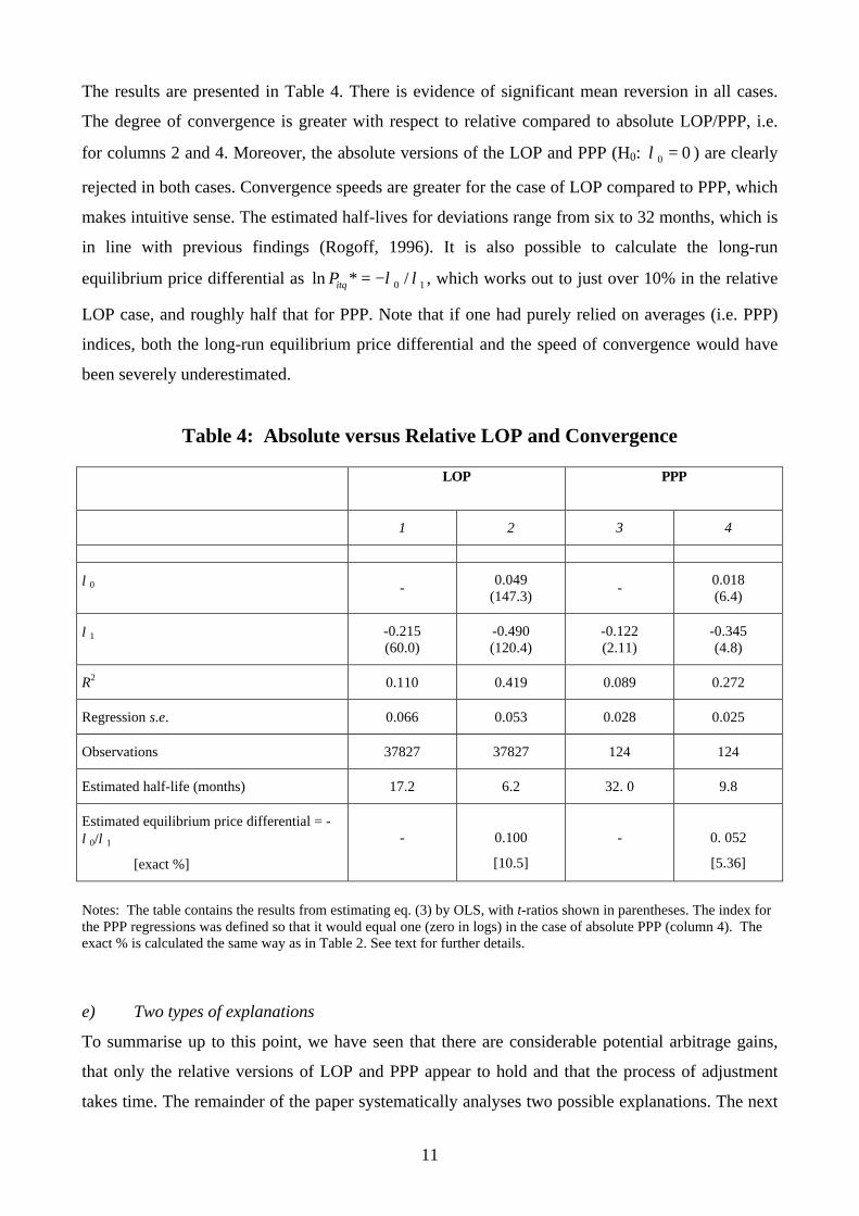
The results are presented in Table 4. There is evidence of significant mean reversion in all cases.
The degree of convergence is greater with respect to relative compared to absolute LOP/PPP, i.e.
for columns 2 and 4. Moreover, the absolute versions of the LOP and PPP (H0: 0 0λ = ) are clearly
rejected in both cases. Convergence speeds are greater for the case of LOP compared to PPP, which
makes intuitive sense. The estimated half-lives for deviations range from six to 32 months, which is
in line with previous findings (Rogoff, 1996). It is also possible to calculate the long-run
equilibrium price differential as 0 1ln * /itqP λ λ= − , which works out to just over 10% in the relative
LOP case, and roughly half that for PPP. Note that if one had purely relied on averages (i.e. PPP)
indices, both the long-run equilibrium price differential and the speed of convergence would have
been severely underestimated.
Table 4: Absolute versus Relative LOP and Convergence
LOP PPP
1 2 3 4
λ0 - 0.049(147.3)
- 0.018(6.4)
λ1 -0.215(60.0)
-0.490(120.4)
-0.122(2.11)
-0.345(4.8)
R2 0.110 0.419 0.089 0.272
Regression s.e. 0.066 0.053 0.028 0.025
Observations 37827 37827 124 124
Estimated half-life (months) 17.2 6.2 32. 0 9.8
Estimated equilibrium price differential = -λ0/λ1
[exact %]
- 0.100
[10.5]
- 0. 052
[5.36]
Notes: The table contains the results from estimating eq. (3) by OLS, with t-ratios shown in parentheses. The index forthe PPP regressions was defined so that it would equal one (zero in logs) in the case of absolute PPP (column 4). Theexact % is calculated the same way as in Table 2. See text for further details.
e) Two types of explanations
To summarise up to this point, we have seen that there are considerable potential arbitrage gains,
that only the relative versions of LOP and PPP appear to hold and that the process of adjustment
takes time. The remainder of the paper systematically analyses two possible explanations. The next

12
section deals with price-setting in segmented markets (PSM), as addressed in the IO literature.
Section 4 analyses the role of arbitrage barriers using the gravity trade model.
To illustrate how these two sets of explanations are related, consider the relationship for an
imperfectly competitive firm between its optimal unconstrained price difference in two markets,
1 2* *P P− , the cost of arbitrage between the two markets, 1,2AC , and the actual price difference
1 2P P− set by the firm. There are two possibilities. In the first case,
1 2 1 2 1,2* * AP P P P C− = − ≤ , (4)
i.e. 1,2AC is too high so that, although arbitrage is possible in principle, the firm will behave like an
unconstrained price-discriminator. This is basically the scenario envisaged by the IO literature
mentioned in the introduction. In the second case
1 2 1,2 1 2* *AP P C P P− = < − , (5)
thus arbitrage costs are low enough to constrain the firm to a maximum price differential of 1,2AC .7
This scenario underlies the analysis of section 4 which exploits the empirical robustness of the
gravity model for bilateral trade flows to proxy the factors determining arbitrage costs.
3. Pricing in segmented markets (PSM)
a) Theoretical considerations
If markets are fully segmented, a profit-maximising monopolist will set the price of its product i in
each market as a mark-up over costs, so that the relative price in two markets will be given by
itj itj itj
itk itk itk
P C
P C
Π=
Π, (6)
where P is the price, C is marginal cost, Π denotes the mark-up factor (= 1 + mark-up), and j, k =
1,...,12 (j ≠ k) are national market indices. All variables are measured in a common currency.
In general, each model-specific mark-up term is a function of demand characteristics and the nature
of competition. Given the specific focus of this paper, a fairly simple structure is employed to
model mark-up variations. The mark-up function for model i in country j is assumed to be (expected
effects are shown above each variable)
7 Due to the block exemption firms may be able to influence 1,2
AC . When they use illegal means, as in the Volkswagen
case, they would have to weigh up the potential gains and costs if they get caught.

13
3 , , , , ,itj itj tj itj itj itj itj itjSCR MSH DOM JAPIMP t E+ + + + − − Π = Π
. (7)
The first term, SCR3tj, is the three-seller concentration ratio (i.e. the market share of the three best
selling manufacturers) and serves as an indication of the overall degree of competition in market j.
The second, MSHitj, is the market share of model i in market j and measures the model-specific
degree of market-power. The shift parameter DOMitj is included to capture the possible premium
consumers attach to domestically produced cars. Next, there is the possibility of higher profit
margins on those imported cars which are subject to trade restrictions. Although this does not affect
imports from other EU countries, there was an agreement until the end of 1999 between the EU and
Japan under which Japanese producers would restrict their imports voluntarily. This applied to five
EU countries: France, Italy, Spain, Portugal and the UK. While it is not clear whether the
restrictions were actually binding (Holmes and Smith, 1995), it is at least possible that this has
raised the mark-up for Japanese imports into these five markets, hence the term JAPIMPitq. As
discussed in Gual (1993), pre-tax prices may be inversely related to tax rates if markets are
segmented. This effect is captured by the inclusion of the tax mark-up, where the tax rate on model i
is given by titj. Lastly, the pricing-to-markets (PTM) literature8 indicates that the mark-up may vary
with the exchange rate, Eitj. If goods are priced locally, exchange rate changes may be less than
completely passed on to the prices of imported goods. The degree of exchange rate pass-through is
therefore a measure of the extent firms have the power to set prices in export markets.
Costs are likely to consist of several components. The first is the cost of manufacturing the good,
the second the cost which arises from selling the good in a given destination market, mainly due to
distribution and marketing, and the third the transportation cost between country-of-origin and
destination-market. Since all differences in manufacturing costs were controlled for when the
adjusted price differential ln itqP was derived in section 2, marginal cost differences can only be due
to local9 and transport cost components. As there is no direct data on these variables, they need to
be proxied. Local costs are assumed to be common to all manufacturers selling in a given market
and thus captured by domestic wages. Differences in transport costs are approximated by relative
distances between markets as in Gual (1993).
8 See for instance Knetter (1993), or the reviews by Menon (1995) and Goldberg and Knetter (1997).9 Since incomplete exchange rate pass-through can also be the result of local cost factors, it is important to includethese to isolate the mark-up effect of exchange rate changes.

14
b) The econometric model
The following regression model of PSM captures all of the above factors in an easily interpretable
way:
1 2 3 4 5
6 7 8 9
ˆln 3
ˆln ln .
itq j k tq itq tq itq itq
itq tq iq itq itq
P b b SCR MSH E DOM JAPIMP
T W RDIS SALES
β β β β β
β β β β ε
= − + + + + +
+ + + + +(8)
Note that as before the subscript q refers to the difference between countries j and k. The variables
are defined as follows (the data and sources are described in the Appendix):
• lnPitq is the quality-adjusted price-differential for model i between national markets j and k at
time t.
• SCR3tq is the difference in the three-seller concentration ratios between markets j and k.
• MSHitq is the difference in the market share of model i in the two markets. This is approximated
by the manufacturer’s annual market share, calculated from sales figures.
• ˆ ln lntq tq tqE E E= − where Etq is defined as country j currency units per unit of country k’s
currency. To render the exchange rate comparable across country-pairs, it is normalised with
respect to its long-term or steady-state value, tqE . The latter is set equal to the 1993-98 mean.
There is incomplete exchange rate pass-through if β3 < 0.
• ˆ (ln ln ) (ln ln )tq tj j tk kW W W W W= − − − . Here Wtj and Wtk are wage indices for the two countries,
and jW and kW the period means. This normalisation makes the country-specific indices
comparable. Both the exchange rate and wage variables are thus logarithmic deviations from
their respective means which, for small values, have the intuitive interpretation of percentage
deviations.
• DOMitq = 1 if (i) the manufacturer’s headquarters or (ii) the production of model i is based in
country j, DOMitq = -1 if either is based in country k, 0 otherwise. Ford and Opel/Vauxhall are
assumed to be ‘domestic’ in both Germany and UK.
• JAPIMPitq = 1 if the car is manufactured in Japan and country j is one of the five countries
(France, Italy, Spain, Portugal, UK) potentially affected by the EU-Japanese agreement,
JAPIMPitq = - 1 if the car is manufactured in Japan and country k is one of the five countries.
• Titq = (1 + titj)/(1 + titk) and captures the effect on pre-tax prices of different levels of taxation.
The model-specific tax factors, 1 + titj, are obtained by dividing the post-tax by pre-tax prices
from the EC’s car price reports.
• RDISiq is the relative distance between country j and the country-of-origin of model i and
between country k and the country-of-origin of model i. For imports from Japan, RDISiq = 1.
15
• SALESitq = is the difference in sales of model i (approximated by manufacturer-specific annual
sales) in the two markets, included to capture possible non-constant returns to scale in domestic
cost factors.
• bj and bk are dummy variables to capture additional market-specific mark-up and cost effects.
• εitq is a stochastic error term.
It is possible that the residuals are correlated across models for a given country-comparison, if there
are aggregate shocks affecting all model comparisons. In this case the efficient estimator is
generalised least squares; moreover, OLS standard errors would be biased. However, as Beck and
Katz (1995) show, feasible generalised least squares can have undesirable consequences and be
inferior to OLS. I therefore use OLS to obtain consistent estimates of the parameters and panel-
corrected standard errors (PCSEs) for inference. The latter take account of the potential cross-
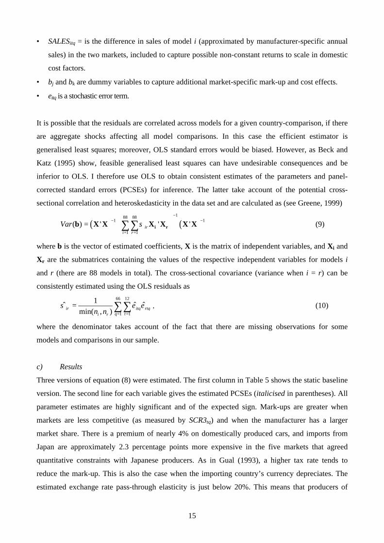
sectional correlation and heteroskedasticity in the data set and are calculated as (see Greene, 1999)
( ) ( )188 88
1 1
1 1
( ) ' ' 'iri r
Var σ−
− −
= =
= ∑∑ i rb X X X X X X (9)
where b is the vector of estimated coefficients, X is the matrix of independent variables, and Xi and
Xr are the submatrices containing the values of the respective independent variables for models i
and r (there are 88 models in total). The cross-sectional covariance (variance when i = r) can be
consistently estimated using the OLS residuals as
66 12
1 1
1ˆ ˆˆ
min( , )ir itq rtqq ti rn n
σ ε ε= =
= ∑∑ , (10)
where the denominator takes account of the fact that there are missing observations for some
models and comparisons in our sample.
c) Results
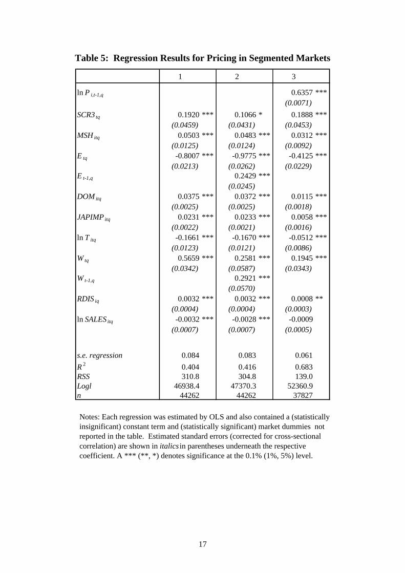
Three versions of equation (8) were estimated. The first column in Table 5 shows the static baseline
version. The second line for each variable gives the estimated PCSEs (italicised in parentheses). All
parameter estimates are highly significant and of the expected sign. Mark-ups are greater when
markets are less competitive (as measured by SCR3tq) and when the manufacturer has a larger
market share. There is a premium of nearly 4% on domestically produced cars, and imports from
Japan are approximately 2.3 percentage points more expensive in the five markets that agreed
quantitative constraints with Japanese producers. As in Gual (1993), a higher tax rate tends to
reduce the mark-up. This is also the case when the importing country’s currency depreciates. The
estimated exchange rate pass-through elasticity is just below 20%. This means that producers of
16
imported models mainly adjust their profit margins to maintain their local currency prices when the
exchange rate changes.
With respect to the cost side, the estimated wage effect suggests that a one percent rise in domestic
labour costs is associated with a 0.57% increase in the relative price. A greater distance to the
country-of-origin also raises costs. The estimated coefficient on lnSALESitq indicates that local
value added (i.e. distribution and marketing) is subject to increasing returns to scale: a doubling of
sales volume is associated with a 0.3% reduction in costs. Note that the regressions in Table 5 also
contain (not explicitly reported) a statistically significant set of market dummies and an
insignificant constant term.
17
Table 5: Regression Results for Pricing in Segmented Markets
1 2 3
ln P i,t-1,q 0.6357 ***(0.0071)
SCR3 tq 0.1920 *** 0.1066 * 0.1888 ***(0.0459) (0.0431) (0.0453)
MSH itq 0.0503 *** 0.0483 *** 0.0312 ***(0.0125) (0.0124) (0.0092)
E tq -0.8007 *** -0.9775 *** -0.4125 ***(0.0213) (0.0262) (0.0229)
E t-1,q 0.2429 ***(0.0245)
DOM itq 0.0375 *** 0.0372 *** 0.0115 ***(0.0025) (0.0025) (0.0018)
JAPIMP itq 0.0231 *** 0.0233 *** 0.0058 ***(0.0022) (0.0021) (0.0016)
ln T itq -0.1661 *** -0.1670 *** -0.0512 ***(0.0123) (0.0121) (0.0086)
W tq 0.5659 *** 0.2581 *** 0.1945 ***(0.0342) (0.0587) (0.0343)
W t-1,q 0.2921 ***(0.0570)
RDIS iq 0.0032 *** 0.0032 *** 0.0008 **(0.0004) (0.0004) (0.0003)
ln SALES itq -0.0032 *** -0.0028 *** -0.0009(0.0007) (0.0007) (0.0005)
s.e. regression 0.084 0.083 0.061
R 2 0.404 0.416 0.683RSS 310.8 304.8 139.0Logl 46938.4 47370.3 52360.9n 44262 44262 37827
Notes: Each regression was estimated by OLS and also contained a (statisticallyinsignificant) constant term and (statistically significant) market dummies notreported in the table. Estimated standard errors (corrected for cross-sectionalcorrelation) are shown in italics in parentheses underneath the respectivecoefficient. A *** (**, *) denotes significance at the 0.1% (1%, 5%) level.
18
The specification in column 2 introduces simple dynamics in form of additional one-period lags of
exchange rates and wages. The resulting estimates suggest that there is some inertia in the response
to exchange rate and wage changes. The initial degree of exchange rate pass-through is now
practically zero, i.e. relative prices initially move one for one with exchange rates, but there is some
reversion a period later. The long-run elasticity of 0.73 is just a little below the static estimate. This
adjustment pattern makes intuitive sense since it is likely that producers initially adopt a wait-and-
see attitude in case a given exchange rate change is only temporary, especially as they are likely to
be covered against unexpected short-run exchange rate fluctuations via forward contracts. The wage
effect is now roughly split in two, the initial elasticity being estimated at 0.26. The long-run
elasticity of 0.55 is practically identical to the static regression result in column 1.
The third set of estimates includes a lagged dependent variable (LDV) to capture more general
incomplete adjustment in the short run. The values in the table are OLS estimates, but instrumental
variable estimation (using the two-period lag of the dependent variable as instrument) was also
tried. The results were nearly identical and since they entailed the loss of one period’s data, it was
decided to present the OLS results here. The estimated adjustment coefficient of 0.64 suggests that
shocks have a half-life of a little over nine months. Most of the estimated long-run effects are
similar to the static version in column 1. The major differences are an increase in the estimated
long-run effects of SCR3tq and exchange rate (now exceeding unity). There is also an increase to
68% in explanatory power. In summary, the estimates in Table 5 support the specification of mark-
up and cost differences in equation (8), including the claim often voiced by manufacturers (ACEA,
1998) that exchange rate fluctuations and differences in indirect taxation lead to price differentials
in the EU car market.
4. The role of arbitrage barriers
a) Theoretical considerations
This section examines to what extent price differences in the EU car market are the result of barriers
to arbitrage trade. This case was described in eq. (5) earlier. The starting point here is that relative
prices and trade incentives are related: the larger are price differences, the greater the potential gains
from trade; and the more trade there is, the smaller will be price differences. It follows that the
factors that inhibit trade are also likely to have an effect on price differences. With respect to trade
impediments a standard distinction is between natural and artificial barriers to trade. Transportation
and transaction costs fall into the first category, and formal trade barriers such as tariffs and quotas
into the second.

19
There is a growing literature which suggests that transaction costs are important for trade. Rauch
(1999), for instance, argues that search costs in international trade lead to ‘trading networks’ which
serve to match international sellers and buyers, particularly in the case of differentiated products.
Such networks will develop most easily when costs are low which will be especially the case when
participants are proximate to each other or have existing ties. Such transaction costs are also likely
to be relevant in our case. For instance, when individual consumers engage in arbitrage they cannot
rely on the official distribution channels, as the VW case has shown. Thus a good example for
costly search is finding a foreign distributor willing to supply the desired car.
Search costs also affect professional suppliers of parallel imports. They are excluded from official
marketing activities by the manufacturers, and thus do not benefit from general information flows
(such as price information) as do official sellers. As a result, they have to spend additional
resources, not only to find potential buyers, but also to convince them that their products are of
equal value to those going through the official channels. This may be necessary in the face of three
widely held perceptions, i.e. that manufacturer warranties do not apply to parallel imports, official
dealers may refuse to service and repair parallel imports and that such cars are of inferior quality.
The first two are factually wrong as warranties apply to the whole of the EU and dealers are legally
obliged to undertake servicing and necessary repairs. As regards the third point, even if there are
differences in specification or equipment levels, these are verifiable and thus prices can be adjusted
accordingly.
The most widely used model to predict trade flows is the gravity model. Its main weakness, that it is
compatible with a variety of theoretical trade models (Deardorff, 1998), turns into its strength here,
since it also encompasses Rauch’s transaction cost view of trade. The basic gravity model relates
trade volume to distance and economic size. It can be readily extended to incorporate other factors
that are thought to affect search costs, such as whether two countries share a common language
and/or border. These variables capture potential information advantages resulting from the absence
of translation needs and the utilisation of general cross-border information flows between
neighbouring countries.
Three further factors that may affect arbitrage costs are considered here.
– The first is technical and applies to the UK and Ireland: right-hand drive. Even though there are
no legal barriers to the use of the ‘wrong’ drive (i.e. right-hand drive in the UK/Ireland or left-hand
drive in the rest of the EU), it is probably more difficult to source a right-hand drive vehicle on the

20
continent and vice versa, if only because they are not kept in stock. One would therefore expect
search and information costs to be higher in such cases.
– The second has to do with the voluntary restrictions on Japanese imports already described
above. Due to the national quota constraints arbitrage trade in Japanese imports has been
particularly affected in the countries concerned. We would therefore expect this to raise ceteris
paribus price differentials for Japanese imports into these markets.
– Third, one of the main benefits of a single European currency is increased price transparency
across national markets. The precise response to the single currency is still uncertain at present, but
the currency union between Belgium and Luxembourg can be used to study its likely effect.
b) The econometric model
These considerations suggest the following model to examine the arbitrage explanation of car price
differentials across the EU:
0 1 2 3 4
5 6 7
ln ln lnitq q itq q q
iq itq q itq
P DIST MSIZE COMMLA COMMBO
RHD JAPARB MU
α α α α α
α α α ε
= + + + +
+ + + +. (11)
The new variables are defined as follows:
• DISTq is the distance between markets j and k.
• itq itj itkMSIZE MSIZE MSIZE= + is the sum of the sales of the manufacturer concerned in the
two markets. This variable is included to capture ‘gravitational’ forces due to market size. We
would expect this scale variable to be negatively correlated with price differentials if the size of
the market for a given model has a positive effect on arbitrage trade.
• COMMLAq = 1 if the two countries concerned share a common language, 0 otherwise.
• COMMBOq = 1 if the two countries concerned share a common border, 0 otherwise.
• RHDiq = 1 if either of the two countries is Ireland or the UK (but not both), 0 otherwise.
• JAPARBitq = 1 if one or both of the two countries concerned belongs to the group of five
affected by voluntary import restrictions from Japan and model i is manufactured in Japan, 0
otherwise.
• MUq = 1 if the country comparison refers to Belgium versus Luxembourg, 0 otherwise.
• Since lnPitq can be positive or negative, but our interest is in explaining absolute differentials,
all the right-hand side variables in eq. (11) are multiplied by -1 for ln 0itqP < .
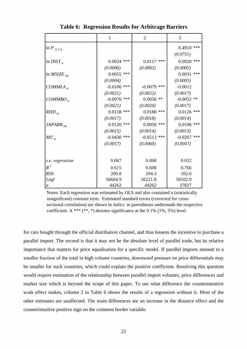
c) Results 1: arbitrage barriers only
OLS results with PCSEs for three versions of eq. (11) are shown in Table 6. The first column lists
the estimates from the static version. All the coefficients are highly significant and have the

21
expected sign, except for the scale factor (measured by MSIZEitq). The estimated distance effect
associates a distance of 1000km with a 2.4% price differential. Country-pairs that share a common
language have price differentials which are a little over one percentage point lower than between
other countries. The common border effect is a little lower at just over three-quarters of a
percentage point. Bigger effects are due to right-hand versus left-hand drive at over one-and-a-half
percentage points, and the Japanese imports effect at 1.2 percentage points. The biggest single
factor reducing arbitrage costs appears to be a common currency at -4.3%, at least in the Belgium-
Luxembourg case.
This leaves the scale factor that is included in the gravity model to capture the influence of income
on the demand for tradables. Something similar was envisaged here, since higher official sales mean
a larger potential market for parallel imports. If there are scale effects, arbitrage costs would be
lowered, thus leading to smaller price differentials. However, the estimated correlation is positive10
and significant. Two possible explanations come to mind. One is that a larger distribution network
(implied by larger sales volumes) lowers relative search costs
10 GDP and total market sales were also tried but gave similar results (both in logarithms and as products). GDP percapita had a negative effect but in those regressions distance also had a negative sign which, incidentally, is also thecase in Haskell and Wolf’s (1999) study of price differentials for IKEA furniture.
22
Table 6: Regression Results for Arbitrage Barriers
1 2 3
ln P i,t-1,q 0.4910 ***(0.0751)
ln DIST q 0.0034 *** 0.0117 *** 0.0020 ***(0.0006) (0.0002) (0.0005)
ln MSIZE itq 0.0055 *** 0.0031 ***(0.0004) (0.0003)
COMMLA q -0.0106 *** -0.0079 *** -0.0012(0.0021) (0.0022) (0.0017)
COMMBO q -0.0076 *** 0.0056 ** -0.0052 **(0.0021) (0.0020) (0.0017)
RHD iq 0.0158 *** 0.0180 *** 0.0126 ***(0.0017) (0.0018) (0.0014)
JAPARB itq 0.0120 *** 0.0058 *** 0.0106 ***(0.0015) (0.0014) (0.0013)
MU q -0.0430 *** -0.0513 *** -0.0267 ***(0.0057) (0.0060) (0.0047)
s.e. regression 0.067 0.068 0.052
R 2 0.615 0.608 0.766RSS 200.8 204.3 102.6Logl 56604.9 56221.8 58102.9n 44262 44262 37827
Notes: Each regression was estimated by OLS and also contained a (statistically insignificant) constant term. Estimated standard errors (corrected for cross-sectional correlation) are shown in italics in parentheses underneath the respective coefficient. A *** (**, *) denotes significance at the 0.1% (1%, 5%) level.
for cars bought through the official distribution channel, and thus lessens the incentive to purchase a
parallel import. The second is that it may not be the absolute level of parallel trade, but its relative
importance that matters for price equalisation for a specific model. If parallel imports amount to a
smaller fraction of the total in high volume countries, downward pressure on price differentials may
be smaller for such countries, which could explain the positive coefficient. Resolving this question
would require estimation of the relationship between parallel import volumes, price differences and
market size which is beyond the scope of this paper. To see what difference the counterintuitive
scale effect makes, column 2 in Table 6 shows the results of a regression without it. Most of the
other estimates are unaffected. The main differences are an increase in the distance effect and the
counterintuitive positive sign on the common border variable.
23
The third version in Table 6 adds a lagged dependent variable to allow for adjustment dynamics.
The estimated long-term effects are very different compared to the static version in column 1. The
major change is that a common language now has a much smaller effect. Some of the other
arbitrage variables gain in influence, such as a common border and the right-hand drive and
Japanese import effects. The estimated speed of adjustment is higher than for the PSM model in the
previous section. Instrumental Variable (IV) estimation was also tried but, again, there was little
difference in the estimated parameters so only OLS estimates are presented here.
The results obtained in this section suggest that the assumption of completely segmented markets is
not supported by this data set. Arbitrage barriers as captured by the gravity model variables are
significantly related to price differentials. In fact, they are even more successful at explaining
variations in price differentials than the PSM model. This is indicated by an R2 of 61% compared to
40% earlier for the static versions, and 77% versus 68% for the dynamic model. But there is still the
possibility that the pricing decisions of firms are not affected by arbitrage barriers. To implement a
proper test of the importance of arbitrage considerations, the next step involves the estimation of the
joint model. If the estimated effect of the PSM variables (as measured by the size of the estimated
coefficients) remains unchanged, there is little to be gained from studying the factors leading to
market segmentation. On the other hand, a reduction in their importance would indicate that firms
do not set their prices independently of arbitrage considerations.
d) Results 2: pricing in segmented markets and and arbitrage barriers
The joint estimates are presented in Table 7. To allow direct comparisons, they are based on the
same three versions of the PSM model shown earlier in Table 5. Since there are a lot of coefficients
to compare, consider first the overall result. The PSM effects are indeed reduced by the inclusion of
the arbitrage variables. For the majority of variables, the estimated long-run effects in

24
Table 7: Combined Regression Results
1 2 3
ln P i,t-1,q 0.4119 ***(0.0061)
ln DIST q 0.0070 *** 0.0070 *** 0.0049 ***(0.0004) (0.0004) (0.0004)
ln MSIZE itq 0.0018 *** 0.0017 *** 0.0011 ***(0.0003) (0.0002) (0.0002)
COMMLA q -0.0049 *** -0.0047 *** -0.0005(0.0014) (0.0014) (0.0014)
COMMBO q 0.0006 0.0010 0.0001(0.0014) (0.0014) (0.0014)
RHD iq 0.0061 *** 0.0065 *** 0.0049 ***(0.0011) (0.0011) (0.0011)
JAPARB itq 0.0059 *** 0.0061 *** 0.0062 ***(0.0012) (0.0012) (0.0011)
MU q -0.0413 *** -0.0414 *** -0.0297 ***(0.0035) (0.0034) (0.0038)
SCR3 tq 0.0450 0.0002 0.0903 **(0.0270) (0.0259) (0.0313)
MSH itq 0.0311 *** 0.0302 *** 0.0260 ***(0.0085) (0.0085) (0.0074)
E tq -0.4520 *** -0.5514 *** -0.3070 ***(0.0130) (0.0162) (0.0161)
E t-1,q 0.1329 ***(0.0147)
DOM itq 0.0169 *** 0.0170 *** 0.0068 ***(0.0017) (0.0017) (0.0015)
JAPIMP itq 0.0112 *** 0.0114 *** 0.0040 **(0.0014) (0.0014) (0.0012)
ln T itq -0.0911 *** -0.0931 *** -0.0402 ***(0.0077) (0.0077) (0.0067)
W tq 0.2819 *** 0.1391 *** 0.1282 ***(0.0200) (0.0353) (0.0236)
W t-1,q 0.1338 ***(0.0343)
RDIS iq 0.0016 *** 0.0016 *** 0.0006 **(0.0002) (0.0002) (0.0002)
ln SALES itq -0.0015 ** -0.0014 ** -0.0007(0.0005) (0.0005) (0.0004)
s.e. regression 0.059 0.059 0.049
R 2 0.702 0.705 0.792RSS 155.5 153.9 91.3Logl 62259.1 62498.0 60314.5n 44262 44262 37827
Notes: Each regression was estimated by OLS and also contained a (statistically insignificant) constant term and (statistically significant) market dummies not reported in the table. Estimated standard errors (corrected for cross-sectional correlation) are shown in italics in parentheses underneath the respective coefficient. A *** (**, *) denotes significance at the 0.1% (1%, 5%) level.
25
Table 7 are less than half those obtained earlier, amounting to 49%, 48% and 42% (on average) of
those in Table 5. The degree of price inertia in response to exchange rate changes, for instance, is
reduced to between -0.42 and -0.52, and the elasticity with respect to domestic labour costs to no
more than 0.28. Clearly, the economic importance of these variables is severely overestimated in
the absence of arbitrage considerations. These reductions apply across all variables in Table 7. It is
unlikely that these are just random fluctuations, since these reductions apply to all variables, there
are no sign reversals, and the estimated coefficients remain significant (with the exception of
SCR3tq in the third column).
What about the arbitrage variables? Most also experience a reduction in their economic significance
as a result of being estimated jointly with the PSM factors. The two exceptions are the monetary
union effect that remains practically unchanged, and distance between markets which even sees its
influence strengthened. The border effect is now small and positive but insignificant. The partial
adjustment coefficient of the dynamic model in column 3 is lower than the previous estimates, with
a half-life of shocks now equal to 4.7 months. The overall explanatory power of the joint regression
model exceeds 70% and rises to nearly 80% in the dynamic version (column 3). The country-
specific effects are not reported individually but are again jointly significant.
To summarise, all variables except for the common border effect appear to significantly affect price
differentials in the European car market in at least one version of the joint estimates. Nevertheless,
some of the estimated effects are small numerically and others, such as the common language
factor, affect only a small fraction of price comparisons. To examine the relative importance of the
various explanatory factors, their average shares in explaining deviations from absolute LOP were
calculated on the basis of the benchmark static regression. For the market share variable, for
instance, this meant calculating the product 2ˆ
itqMSHβ for all observations and then taking the mean
absolute value. For each variable its contribution is then calculated as the percentage share in the
total for all variables. The reason why this measure was preferred to an R2 based decomposition by
variable11 is that the latter concerns deviations from the mean, whereas our main interest is on
absolute deviations from zero.
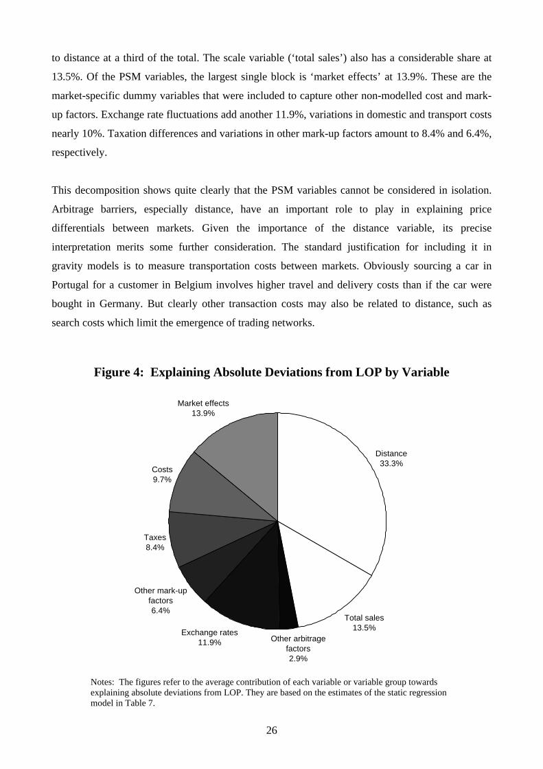
The results are presented in Figure 4. Each pie segment reflects the percentage contribution of the
particular variable (or group of variables) to explaining the absolute deviations from LOP observed
in the data. Nearly half the explanatory power comes from the arbitrage factors, most of it attributed
11 One obtains a qualitatively similar picture from a variance decomposition, but the relative importance of arbitragefactors is even greater then.
26
to distance at a third of the total. The scale variable (‘total sales’) also has a considerable share at
13.5%. Of the PSM variables, the largest single block is ‘market effects’ at 13.9%. These are the
market-specific dummy variables that were included to capture other non-modelled cost and mark-
up factors. Exchange rate fluctuations add another 11.9%, variations in domestic and transport costs
nearly 10%. Taxation differences and variations in other mark-up factors amount to 8.4% and 6.4%,
respectively.
This decomposition shows quite clearly that the PSM variables cannot be considered in isolation.
Arbitrage barriers, especially distance, have an important role to play in explaining price
differentials between markets. Given the importance of the distance variable, its precise
interpretation merits some further consideration. The standard justification for including it in
gravity models is to measure transportation costs between markets. Obviously sourcing a car in
Portugal for a customer in Belgium involves higher travel and delivery costs than if the car were
bought in Germany. But clearly other transaction costs may also be related to distance, such as
search costs which limit the emergence of trading networks.
Figure 4: Explaining Absolute Deviations from LOP by Variable
Distance33.3%
Total sales13.5%
Other arbitrage factors2.9%
Exchange rates11.9%
Other mark-up factors6.4%
Taxes8.4%
Costs9.7%
Market effects13.9%
Notes: The figures refer to the average contribution of each variable or variable group towardsexplaining absolute deviations from LOP. They are based on the estimates of the static regressionmodel in Table 7.
27
5. Limitations and outlook
Not all variations in prices can be explained by our model. Nearly thirty percent of variations
around the mean are unexplained in the static regression. In terms of deviations from LOP, the
mean of absolute residuals translates into an average unexplained price differential of 4.7%. This
remainder is likely to be the result of several factors. There is bound to be some random noise in the
data. Another potential reason is imperfect measurement, in terms of both explanatory and
dependent variables. This not only applies to the domestic and transport cost proxies, but also to
exchange rates since the nominal exchange rate may not be the best measure of that used internally
for price-setting by multinational companies.
Another data limitation is the use of list prices rather than actual transaction prices that are set by
individual dealers. Buyers frequently obtain cash discounts or buy cars that are discounted
indirectly when optional extras are added below cost. This may generate noise in the data but is
unlikely to lead to serious biases. If any, the most likely candidates would appear to be the
exchange rate and labour cost effects. It may be that dealer discounts are larger when the importing
country’s currency appreciates. In this case the degree of exchange rate pass-through would be
understated. Similarly, if higher labour costs mean smaller discounts, the effect of labour cost
differences would be underestimated. The arbitrage factors, on the other hand, are unlikely to be
affected, unless discounts are set nationally and differ systematically with distance etc. This is
unlikely, since even within national markets the difference between list and transaction prices
generally depends on the bargaining process between individual buyers and dealers.
This leaves two essentially political decisions which are likely to influence the future of price
differentiation in the European car market. The first is the European Commission’s own policy
towards the industry: the block exemption. Since this enables manufacturers to interfere with the
arbitrage process it is likely to generate additional deviations from LOP partly responsible for those
remaining 4.7% not explained here. There are probably few welfare grounds in favour of extending
it beyond 2002. Nevertheless, the manufacturers are likely to lobby hard to persuade the European
Commission to do just that. The second is the single European currency. If the Belgium-
Luxembourg example is a valid guide to its likely impact, then the single currency will help reduce
price differentials in the medium to long run.

28
6. Conclusions
The analysis presented in this paper has used micro-level price data to examine why there are
deviations from the law of one price in the European car market. Within-period price differences
were shown to be substantial both in relative and absolute terms, and there has been no tendency for
average price differentials to decline during the single market period. There is no evidence that the
differences are due to variations in specification or equipment levels. Although absolute LOP is
strongly rejected, there is evidence of convergence to the relative version of the LOP. To explain
these findings, the paper contrasts two sets of explanations: (i) price-setting behaviour in fully
segmented markets, and (ii) the role played by arbitrage barriers. The first set of variables attempts
to explain differences in mark-up and marginal costs across markets. Differences in market- and
model-specific mark-up determinants are systematically related to price-differentials, as are
differences in local and transport costs.
However, the importance of price-setting variables is severely overestimated when arbitrage factors
are not controlled for. The joint model adds a variety of proxies for arbitrage costs based on the
gravity model. Their inclusion reduces the economic significance of mark-up and cost differences
by more than 50%. Statistically, though, they remain significant determinants of price differentials.
Of the variables proxying arbitrage costs, distance makes the largest overall contribution to
explaining LOP deviations. Having a common language had a significant effect for the country-
pairs affected. The quantitative restrictions on Japanese imports still in place during the sample
period also raised price differentials, both through their influence on manufacturer’s mark-ups and
through the extra impediments placed on arbitrage trade in these vehicles. The biggest single effect
at over four percentage points was estimated for the monetary union between Belgium and
Luxembourg, even after controlling for other factors such as their common border and shared
language.
This evidence on prices suggests that the single market project is not yet complete. Some of the
welfare gains originally promised are still to be realised. Concerning the car sector, the most
immediate and obvious policy recommendation must be for the Commission’s competition policy
to change. The block exemption has given manufacturers too much leverage over the sale of their
cars and should not be extended beyond 2002, if the EU is serious about greater market integration.
But there are also more general conclusions to be drawn. If the findings in this paper are to be
believed, the single currency will make a significant contribution to the lowering of price
differentials by increasing transparency and thereby lowering cross-border transaction costs. There
is no reason to expect this not to apply to other traded goods in the EU.
29
Appendix: Description of the Data Set
Manufacturers and Models (Source: Car prices in the European Union):
Alfa-Romeo: 33/145, 155/156, 164.Audi: A3, 80/A4, 100/A6, A8.BMW: 3-Series, 5-Series, 7-Series.Citroen: AX/Saxo, ZX/Xsara, Xantia,
Evasion/Synergie.Daihatsu: Applause, Charade, Gran Move.Fiat: Cinquecento/Seicento, Uno/Punto,
Tipo/Bravo, Tempra/Marea, Croma.
Ford: Fiesta, Escort/Focus, Mondeo, Scorpio.
Honda: Civic, Accord.Lancia: Y, Dedra, Thema/Kappa.Land Rover: Discovery, Range Rover,
Freelander.Mazda: 121, Demio, 323, 626.Mercedes: 190/C-Class, E-Class, S-Class.Mitsubishi: Colt, Galant, Carisma, Pajero.
Nissan: Micra, Sunny/Almera, Primera.
Opel: Corsa, Astra, Vectra, Omega.Peugeot: 106, 205/206, 306, 405/406,
806.Renault: Twingo, Clio, 19/Megane,
21/Laguna, Safrane, Espace.Rover: MGF, 111, 214, 414/416, 620,
820.Seat: Marbella/Arosa, Ibiza,
Cordoba, Toledo.Subaru: Legacy, Forester.Suzuki: Swift, Baleno.Toyota: Carina/Avensis, Starlet,
Corolla.Volvo: 440/S40, 850/S70, S80,
940/960.VW: Polo, Golf, Vento/Bora, Passat.
Time Periods: 1st May and 1st November, 1993 – 1998.
Markets: Belgium (B), France (F), Germany (D), Ireland (Ire), Italy (I), Luxembourg (L),Netherlands (NL), Portugal (P), Spain (E), UK (UK). 1995-98: Austria (A), Sweden (S).
Distance: Since there is no unique measure of distance between countries, the driving distance(Collins Road Atlas for Europe 1995) between the ‘major’ cities closest to each other in the twocountries was used. The ‘major’ cities are: A: Innsbruck, Vienna. B: Bruxelles. D: Hamburg,Cologne, Munich. E: Madrid, Barcelona. F: Paris, Lyon, Marseilles. Ire: Dublin. I: Rome, Milan. L:Luxembourg. NL: Amsterdam, The Hague. P: Lisbon, Porto. S: Stockholm, Malmö. UK: London,Manchester.
Common language: A-D, A-L, B-F, B-L, B-NL, D-L, F-L, Ire-UK, L-NL.
Common border: A-D, A-I, B-F, B-L, B-NL, D-F, D-L, D-NL, E-F, E-P, F-L.
Exchange Rates: IMF International Financial Statistics; end-of-period values for April (for the 1stMay price data) and October (for the 1st November price data).
Wages: Monthly series from the OECD’s Main Economic Indicators unless indicated. For monthlydata, the months of April and October were used; for quarterly series, the second and fourth quarter.A: hourly rates, industry. B: hourly rates, manufacturing. D: hourly earnings, manufacturing. E:hourly earnings, all activities (quarterly). F: labour costs (IMF). Ire: hourly earnings, manufacturing(quarterly). I: hourly rates, industry. L: monthly earnings, industry. NL: hourly wage rates,manufacturing. P: hourly wages, industry (quarterly, Eurostat). S: hourly earnings, manufacturing.UK: weekly earnings, whole economy.
Sales: Annual data from various issues of Motor Industry of Great Britain: World AutomotiveStatistics and Monthly Statistical Review, both published by the Society of Motor Manufacturersand Traders Ltd., London. Because the logarithm of sales was taken for some variables, all zerosales figures were set equal to one.
30
References
ACEA (1998). No uniform car prices without single currency and tax harmonisation. ACEA PressRelease, 13th February 1998. http://www.acea.be/acea/130298.html.
ACEA (1999). Price differences for cars smaller than for other products. ACEA Press Release, 1st
February 1999. http://www.acea.be/acea/010299.html.Beck, N. and Katz, J. (1995). What to do (and not to do) with time-series cross-section data.
American Political Science Review, 89, 634-647.BEUC (1998). A single price for a single currency? BEUC Press Release, 21st December 1998,
Bruxelles.Campa, J. and Wolf, H. (1997). Is real exchange rate mean reversion caused by arbitrage ? NBER
Working Paper No. 6162. Washington: NBER.Cumby, R. (1996). Forecasting exchange rates and relative prices with the hamburger standard: is
what you want what you get with McParity? NBER Working Paper No. 5675. Washington,D.C.: NBER.
Deardorff, A. (1998). Determinants of bilateral trade: does gravity work in a neoclassical world ? InJ. Frankel (Ed.). The Regionalization of the World Economy. Chicago: University of ChicagoPress and NBER.
Dornbusch, R. (1988). Purchasing power parity. In The New Palgrave: A Dictionary of Economics.New York: Stockton Press.
Edison, H., Gagnon, J. and W. Melick (1997). Understanding the empirical literature on purchasingpower parity: the post-Bretton Woods era. Journal of International Money and Finance, 16, 1-17.
Engel, C. (1993). Real exchange rates and relative prices. Journal of Monetary Economics, 32, 35-50.
Engel, C. (1996). Long-run PPP may not hold after all. NBER Working Paper No. 5646.Washington, D.C.: NBER.
Engel, C. and J. Rogers (1996). How wide is the border ? American Economic Review, 86, 1112-1125.
European Commission. Car Prices in the European Union. Bruxelles: Directorate-General IV-Competition. (various issues)
European Commission (1995). Car Price Differentials in the European Union on 1 May 1995. Pressrelease IP/95/768, 24 July 1995, Bruxelles.
Frankel, J. and Rose, A. (1996). A panel project on purchasing power parity: mean reversion withinand between countries. Journal of International Economics, 40, 209-224.
Froot, K., Kim, M. and Rogoff, K. (1995). The law of one price over 700 years. NBER WorkingPaper No. 5132. Washington: NBER.
Froot, K. and Rogoff, K. (1995). Perspectives on PPP and long-run real exchange rates. In G.Grossman and K. Rogoff (Eds), Handbook of International Economics, vol. III, Amsterdam:Elsevier Science, 1647-88.
Ghosh, A. and Wolf, H. (1994). Pricing in international markets: lessons from The Economist.NBER Working Paper No. 4806. Washington, D.C.: NBER.
Goldberg, P. and Knetter, M. (1997). Goods prices and exchange rates: what have we learned?Journal of Economic Literature, 35, 1243-72.
Goldberg, P. and Verboven, F. (1998). The evolution of price discrimination in the European carmarket. NBER Working Paper No. 6818. Washington, D.C.: NBER.
Greene, W. (1999). Econometric Analysis, 4th Edition. New Jersey: Prentice Hall.Gual, J. (1993). An econometric analysis of price differentials in the EEC automobile market.
Applied Economics, 25, pp. 599-607.Haskell, J. and Wolf, H. (1999). Why does the law of one price fail? A case study. CEPR
Discussion Paper No. 2187. London: CEPR.

31
Helliwell, J. (1998). How Much Do National Borders Matter? Washington, D.C.: BrookingsInstitution Press.
Holmes, P. and Smith, A. (1995). Trade, Competition and Industrial Policy: Conflicts of Aims andInstruments in the Car Sector. University of Sussex, Brighton: European Institute.
Jenkins, M. (1997). Cities, borders, distances, non-traded goods and purchasing-power parity.Oxford Bulletin of Economics and Statistics, 59, 203-212.
Kirman, A. and Schueller, N. (1990). Price leadership and discrimination in the European carmarket. Journal of Industrial Economics, 34, 69-91.
Knetter, M. (1989). Price discrimination by U.S. and German exporters. American EconomicReview, 79, 198-210.
Knetter, M. (1993). International comparisons of pricing to markets behaviour. American EconomicReview, 83, 473-486.
Knetter, M. (1997). The segmentation of international markets: evidence from The Economist.NBER Working Paper No. 5878. Washington, D.C.: NBER.
Lothian, J. and Taylor, M. (1996). Real exchange rate behavior: the recent float from theperspective of the past two centuries. Journal of Political Economy, 104, 488-509.
Lutz, M. (2000). EU commission versus Volkswagen: new evidence on price differentiation in theEuropean car market. Review of Industrial Organization, 15, forthcoming.
Mertens, Y. and Ginsburgh, V. (1985). Product differentiation and price discrimination in theEuropean community: the case of automobiles. Journal of Industrial Economics, 34, 151-165.
Menon, J. (1995). Exchange rate pass-through. Journal of Economic Surveys, 9, 197-232.Obstfeld, M. and Taylor, A. (1997). Nonlinear aspects of goods-market arbitrage and adjustment:
Heckscher’s commodity points revisited. NBER Working Paper No. 6053. Washington, D.C.:NBER.
O’Connell, P. (1998). The overvaluation of purchasing power parity. Journal of InternationalEconomics, 44, 1-19.
Ong, L. (1997). Burgernomics: the economics of the Big Mac standard. Journal of InternationalMoney and Finance, 16, 865-78.
Panos, M., Nobay, M. and Peel, D. (1997). Transactions costs and nonlinear adjustment in realexchange rates: an empirical investigation. Journal of Political Economy, 105, 862-879.
Papell, D. (1997). Searching for stationarity: purchasing power parity under the current float.Journal of International Economics, 43, 313-332.
Rauch, J. (1999). Networks versus markets in international trade. Journal of InternationalEconomics, 48, 7-35.
Rogoff, K. (1996). The purchasing power parity puzzle. Journal of Economic Literature, 34, 647-668.
Smith, A. and Venables, A. (1988). Completing the internal market in the European Community:some industry simulations. European Economic Review, 31, 89-96.
Verboven, F. (1996). International price discrimination in the European car market. Rand Journal ofEconomics, 27, 240-268.