Embed Size (px)
Citation preview

Neural Networks Demystified
Louise Francis, FCAS, MAAA
253

Title: Neural Networks Demystified by Louise Francis
Francis Analytics and Actuarial Data Mining, Inc.
Abstract: This paper will introduce the neural network technique of analyzing data as a generalization of more familiar linear models such as linear regression. The reader is introduced to the traditional explanation of neural networks as being modeled on the functioning of neurons in the brain. Then a comparison is made of the structure and function of neural networks to that of linear models that the reader is more familiar with. The paper will then show that backpropagation neural networks with a single hidden layer are universal function approximators. The paper will also compare neural networks to procedures such as Factor Analysis which perform dimension reduction. The application of both the neural network method and classical statistical procedures to insurance problems such as the prediction of frequencies and severities is illustrated.
One key criticism of neural networks is that they are a "black box". Data goes into the "black box" and a prediction comes out of it, but the nature of the relationship between independent and dependent variables is usually not revealed.. Several methods for interpreting the results of a neural network analysis, including a procedure for visualizing the form of the fitted function will be presented.
Acknowledgments: The author wishes to acknowledge the following people who reviewed this paper and provided many constructive suggestions: Patricia Francis-Lyon, Virginia Lambert, Francis Murphy and Christopher Yaure
254

Neural Networks Demystified
Introduction
Artificial neural networks are the intriguing new high tech tool for finding hidden gems in data. They belong to a broader category o f techniques for analyzing data known as data mining. Other widely used tools include decision trees, genetic algorithms, regression splines and clustering. Data mining techniques are used to find patterns in data. Typically the data sets are large, i.e. have many records and many predictor variables. The number of records is typically at least in the tens of thousands and the number of independent variables is often in the hundreds. Data mining techniques, including neural networks, have been applied to portfolio selection, credit scoring, fraud detection and market research. When data mining tools are presented with data containing complex relationships they can be trained to identify the relationships. An advantage they have over classical statistical models used to analyze data, such as regression and ANOVA, is that they can fit data where the relation between independent and dependent variables is nonlinear and where the specific form of the nonlinear relationship is unknown.
Artificial neural networks (hereafter referred to as neural networks) share the advantages just described with the many other data mining tools. However, neural networks have a longer history of research and application. As a result, their value in modeling data has been more extensively studied and better established in the literature (Potts, 2000). Moreover, sometimes they have advantages over other data mining tools. For instance, decisions trees, a method of splitting data into homogenous clusters with similar expected values for the dependent variable, are often less effective when the predictor variables are continuous than when they are categorical. I Neural networks work well with both categorical and continuous variables.
Neural Networks are among the more glamorous of the data mining techniques. They originated in the artificial intelligence discipline where they are often portrayed as a brain in a computer. Neural networks are designed to incorporate key features of neurons in the brain and to process data in a manner analogous to the human brain. Much of the terminology used to describe and explain neural networks is borrowed from biology. Many other data mining techniques, such as decision trees and regression splines were developed by statisticians and are described in the literature as computationally intensive generalizations of classical linear models. Classical linear models assume that the functional relationship between the independent variables and the dependent variable is linear. Classical modeling also allows linear relationship that result from a transformation of dependent or independent variables, so some nonlinear relationships can be approximated. Neural networks and other data mining techniques do not require that the relationships between predictor and dependent variables be linear (whether or not the variables are transformed).
Salford System's course on Advanced CART, October 15, 1999.
255

The various data mining tools differ in their approach to approximating nonlinear functions and complex data structures. Neural networks use a series of neurons in what is known as the hidden layer that apply nonlinear activation functions to approximate complex functions in the data. The details are discussed in the body of this paper. As the focus of this paper is neural networks, the other data mining techniques will not be discussed further.
Despite their advantages, many statisticians and actuaries are reluctant to embrace neural networks. One reason is that they are a "black box". Because of the complexity of the functions used in the neural network approximations, neural network software typically does not supply the user with information about the nature of the relationship between predictor and target variables. The output of a neural network is a predicted value and some goodness of fit statistics. However, the functional form of the relationship between independent and dependent variables is not made explicit. In addition, the strength of the relationship between dependent and independent variables, i.e., the importance of each variable, is also often not revealed. Classical models as well as other popular data mining ~echniques, such as decision trees, supply the user with a functional description or map of the relationships.
This paper seeks to open that black box and show what is happening inside the neural networks. While some of the artificial intelligence terminology and description of neural networks will be presented, this paper's approach is predominantly from the statistical perspective. The similarity between neural networks and regression will be shown. This paper will compare and contrast how neural networks and classical modeling techniques deal with three specific modeling challenges: 1) nonlinear functions, 2) correlated data and 3) interactions. How the output of neural networks can be used to better understand the relationships in the data will then be demonstrated.
Tvoes of Neural Networks A number of different kinds of neural networks exist. This paper will discuss feedforward neural networks with one hidden layer. A feedforward neural network is a network where the signal is passed from an input layer of neurons through a hidden layer to an output layer of neurons. The function of the hidden layer is to process the information from the input layer. The hidden layer is denoted as hidden because it contains neither input nor output data and the output of the hidden layer generally remains unknown to the user. A feedforward neural network can have more than one hidden layer. However such networks are not common. The feedforward network with one hidden layer is one of the most popular kinds of neural networks. It is historically one of the older neural network techniques. As a result, its effectiveness has been established and software for applying it is widely available. The feedforward neural network discussed in this paper is known as a Multilayer Perceptron (MLP). The MLP is a feedforward network which uses supervised learning. The other popular kinds of feedforward networks often incorporate unsupervised learning into the training. A network that is trained using supervised learning is presented with a target variable and fits a function which can be used to predict the target variable. Alternatively, it may classify records into levels of the target variable when the target variable is categorical.
256

This is analogous to the use of such statistical procedures as regression and logistic regression for prediction and classification. A network trained using unsupervised learning does not have a target variable. The network finds characteristics in the data, which can be used to group similar records together. This is analogous to cluster analysis in classical statistics. This paper will discuss only the former kind of network, and the discussion will be limited to a feedforward MLP neural network with one hidden layer. This paper will primarily present applications of this model to continuous rather than discrete data, but the latter application will also be discussed.
Structure of a Feedforward Neural Network
Figure I displays the structure o f a feedforward neural network with one hidden layer. The first layer contains the input nodes. Input nodes represent the actual data used to fit a model to the dependent variable and each node is a separate independent variable. These are connected to another layer of neurons called the hidden layer or hidden nodes, which modifies the data. The nodes in the hidden layer connect to the output layer. The output layer represents the target or dependent variable(s). It is common for networks to have only one target variable, or output node, but there can be more. An example would be a classification problem where the target variable can fall" into one of a number of categories. Sometimes each of the categories is represented as a separate output node.
As can be seen from the Figure 1, each node in the input layer connects to each node in the hidden layer and each node in the hidden layer connects to each node in the output layer.
Figure 1
Three Layer Feedforward Neural Network
Inpul Hidden Ouq~t
Layer LayeT LIar
(Inpul Data) (Processes D*ta) (Predicted Value)
257

This structure is viewed in the artificial intelligence literature as analogous to that o f biological neurons. The arrows leading to a node are like the axons leading to a neuron. Like the axons, they carry a signal to the neuron or node. The arrows leading away from a node are like the dendrites of a neuron, and they carry a signal away from a neuron or node. The neurons of a brain have far more complex interactions than those displayed in the diagram, however the developers of neural networks view neural networks as abstracting the most relevant features o f neurons in the human brain.
Neural networks "learn" by adjusting the strength of the signal coming from nodes in the previous layer connecting to it. As the neural network better learns how to predict the target value from the input pattern, each o f the connections between the input neurons and the hidden or intermediate neurons and between the intermediate neurons and the output neurons increases or decreases in strength. A function called a threshold or activation function modifies the signal coming into the hidden layer nodes. In the early days o f neural networks, this function produced a value o f I or 0, depending on whether the signal from the prior layer exceeded a threshold value. Thus, the node or neuron would only "fire" if the signal exceeded the threshold, a process thought to be similar to that o f a neuron. It is now known that biological neurons are more complicated than previously believed. A simple all or none rule does not describe the behavior o f biological neurons, Currently, activation functions are typically sigmoid in shape and can take on any value between 0 and 1 or between -1 and 1, depending on the particular function chosen. The modified signal is then output to the output layer nodes, which also apply activation functions. Thus, the information about the pattern being learned is encoded in the signals carried to and from the nodes. These signals map a relationship between the input nodes or the data and the output nodes or dependent variable.
Examole 1: Simple Example o f Fitting a Nonlinear Function A simple example will be used to illustrate how neural networks pcrtbma nonlinear function approximations. This example will provide detail about the activation functions in the hidden and output layers to facilitate an understanding of how neural networks work.
In this example the true relationship between an input variable X and an output variable Y is exponential and is o f the following form:
X
Y = e : +~:
Where:
258

- N(0,75)
X - N(12,.5) and N (It, o) is understood to denote the Normal probability distribution with parameters It, the mean o f the distribution and o, the standard deviation o f the distribution.
A sample o f one hundred observations o f X and Y was simulated. A scatterplot o f the X and Y observations is shown in Figure 2. It is not clear from the scatterplot that the relationship between X and Y is nonlinear. The scatterplot in Figure 3 displays the "true" curve for Y as well as the random X and Y values.
Figure 2
8O0
6OO
>..
4O0
2OO
11
: : = : :
. : . : : - * :
: = ; - . . . . .
12 X
13
259

Figure 3
5OO
IO0
Scatterplot of Y and X with "True" Y
115 120 125
X
1 3 0
A simple neural network with one hidden layer was fit to the simulated data. In order to compare neural networks to classical models, a regression curve was also fit. The result o f that fit will be discussed after the presentation o f the neural network results. The structure o f this neural network is shown in Figure 4.
Figure 4
Simple Neural Network Example with One Hidden Node
0 +e +4
Input Hidden Oulput
Layer Layer Layer
260
As neural networks go, this is a relatively simple network with one input node. In biological neurons, electrochemical signals pass between neurons. In neural network analysis, the signal between neurons is simulated by software, which applies weights to the input nodes (data) and then applies an activation function to the weights.
Neuron signal of the biological neuron system --) Node weights o f neural networks
The weights are used to compute a linear sum of the independent variables. Let Y denote the weighted sum:
Y = w o + w~ * X~ + w 2 X 2... + w X ,
The activation function is applied to the weighted sum and is typically a sigmoid function. The most common of the sigmoid functions is the logistic function:
1 f ( Y ) -
i + e -r
The logistic function takes on values in the range 0 to 1. Figures 5 displays a typical logistic curve. This curve is centered at an X value of 0, (i.e., the constant w0 is 0). Note that this function has an inflection point at an X value o f 0 and f (x) value of .5 , where it shifts from a convex to a concave curve. Also note that the slope is steepest at the inflection point where small changes in the value of X can produce large changes in the value of the function. The curve becomes relatively flat as X approaches both ! and -1.
Figure 5
I o
oe
O6
O4
O1
O0
Logistic Function ]
X * * °X
• a a 6 ~ 4 a 2 O0 02 04 OS OS 10 X
261

Another sigmoid function often used in neural networks is the hyperbolic tangent function which takes on values between -1 and 1:
e r _ e - v
f ( Y ) e r + e -r
In this paper, the logistic function will be used as the activation function. The Multilayer Perceptron is a multilayer feedforward neural network with a sigmoid activation function.
The logistic function is applied to the weighted input. In this example, there is only one input, therefore the activation function is:
1 h = f ( X ; wo, w I ) = f ( w 0 + W l X ) = 1 + e -tw°" +WlX )
This gives the value or activation level of the node in the hidden layer. Weights are then applied to the hidden node:
w2 +w3h
The weights w0 and wz are like the constants in a regression and the weights wm and w3 are like the coefficients in a regression. An activation function is then applied to this "signal" coming from the hidden layer:
1 o = f ( h ; w 2 , w 3 ) = 1 + e -(w~ +w3h)
The output function o for this particular neural network with one input node and one hidden node can be represented as a double application of the logistic function:
f ( f ( X ; Wo, w, ); w~, w, ) - (w l +w4 i÷ e ,.o,,1 ~" l + e
It will be shown later in this paper that the use of sigrnoid activation functions on the weighted input variables, along with the second application of a sigmoid, function by the output node is what gives the MLP the ability to approximate nonlinear functions.
One other operation is applied to the data when fitting the curve: normalization. The dependent variable X is normalized. Normalization is used in statistics to minimize the impact of the scale of the independent variables on the fitted model. Thus, a variable with values ranging from 0 to 500,000 does not prevail over variables with values ranging from 0 to 10, merely because the former variable has a much larger scale.
262

Various software products will perform different normalization procedures. The software used to fit the networks in this paper normalizes the data to have values in the range 0 to 1. This is accomplished by subtracting a constant from each observation and dividing by a scale factor. It is common for the constant to equal the minimum observed value for X in the data and for the scale factor to equal the range of the observed values (the maximum minus the minimum). Note also that the output function takes on values between 0 and 1 while Y takes on values between -oo and +oo (although for all practical purposes, the probability of negative values for the data in this particular example is nil). In order to produce predicted values the output, o, must be renormalized by multiplying by a scale factor (the range of Y in our example) and adding a constant (the minimum observed Y in this example).
Fitting the Curve The process of finding the best set of weights for the neural network is referred to as training or learning. The approach used by most commercial software to estimate the weights is backpropagation. Each time the network cycles through the training data, it produces a predicted value for the target variable. This value is compared to the actual value for the target variable and an error is computed for each observation. The errors are "fed back" through the network and new weights are computed to reduce the overall error. Despite the neural network terminology, the training process is actually a statistical optimization procedure. Typically, the procedure minimizes the sum of the squared residuals:
M i n ( E ( Y - 17) 2 )
Warner and Misra (Warner and Misra, 1996) point out that neural network analysis is in many ways like linear regression, which can be used to fit a curve to data. Regression coefficients are solved for by minimizing the squared deviations between actual observations on a target variable and the fitted value. In the case of linear regression, the curve is a straight line. Unlike linear regression, the relationship between the predicted and target variable in a neural network is nonlinear, therefore a closed form solution to the minimization problem does not exist. In order to minimize the loss function, a numerical technique such as gradient descent (which is similar to backpropagation) is used. Traditional statistical procedures such as nonlinear regression, or the solver in Excel use an approach similar to neural networks to estimate the parameters of nonlinear functions. A brief description of the procedure is as follows:
1. Initialize the neural network model using an initial set of weights (usually randomly chosen). Use the initialized model to compute a fitted value for an observation.
2. Use the difference between the fitted and actual value on the target variable to compute the error.
263

3. Change the weights by a small amount that will move them in the direction of a smaller error
• This involves multiplying the error by the partial derivative of the function being minimized with respect to the weights. This is because the partial derivative gives the rate of change with respect to the weights. This is then multiplied by a factor representing the "learning rate" which controls how quickly the weights change. Since the function being approximated involves logistic functions of tbe weights of the output and hidden layers, multiple applications of the chain rule are needed. While the derivatives are a little messy to compute, it is straightforward to incorporate them into software for fitting neural networks.
4. Continue the process until no further significant reduction in the squared error can be obtained
Further details are beyond the scope of this paper. However, more detailed information is supplied by some authors (Warner and Misra, 1996, Smith, 1996). The manuals of a number of statistical packages (SAS Institute, 1988) provide an excellent introduction to several numerical methods used to fit nonlinear functions.
Fitting, the Neural Network For the more ambitious readers who wish to create their own program for fitting neural networks, Smith (Smith, 1996) provides an Appendix with computer code for constructing a backpropagation neural network. A chapter in the book computes the derivatives mentioned above, which are incorporated into the computer code.
However, the assumption for the purposes of this paper is that the overwhelming majority of readers will use a commercial sottware package when fitting neural networks. Many hours of development by advanced specialists underlie these tools. Appendix 1 discusses some of the software options available for doing neural network analysis.
The Fitted Curve: The parameters fitted by the neural network are shown in Table 1.
Table 1 WO Wl
Input Node to Hidden Node -3.088 3.607 Hidden Node to Output Node -1.592 5.281
264

To produce the fitted curve from these coefficients, the following procedure must be used:
1. Normalize each xi by subtracting the minimum observed value 2 and dividing by the scale coefficient equal to the maximum observed X minus the minimum observed X. The normalized values will be denoted X*.
2. Determine the minimum observed value for Y and the scale coefficient for y3. 3. For each normalized observation x*~ compute
1 h ( x *i ) = ! + e - I -3"088+ j
4. For each h (x'i) compute
1 o ( h ( x * i ) ) 1 + e -~-Isg~,5281h~x'"
Compute the estimated value for each yi by multiplying the normalized value from the output layer in step 4 by the Y scale coefficient and adding the Y constant. This value is the neural network's predicted value for Yi.
Table 2 displays the calculation for the first 10 observations in the sample.
2 10.88 in this example. The scale parameter is 2.28 3 In this exlmple the Y minimum was 111.78 ~ the scale parameter was 697.04
265

Table 2
(1) (2) (3) (4) (5) (8) (7) (8) Input Pattern Weighted X
X Y Normalized X Input Logistic(Wt X) Weighted Node 2 Logistic Rescaled Predicted ((1)-10.88)12.28 -3,088*3.607"(3) ll(l*exp(-(4))) -1.5916+5.2814"(5) 1/(l+exp(-(6))) 697.04"(7)+111.78
t~
12.16 665.0 0.5613 -1.0634 0.2567 -0.2361 0.4413 419.4 11.72 344.6 0.3704 -1,7518 0.1478 -0.6109 0,3077 326.3 11.39 281.7 0.2225 -2.2854 0,0923 -1.1039 0.2490 285.3 12.02 423.9 0.4999 -1.2850 0.2167 -0.4471 0,3900 383.7 12.63 519.4 0.7679 -0.3184 0.4211 0,6323 0,5530 566.9 11.19 366.7 0,1359 -2.5978 0.0693 -1.2257 0,2269 270.0 13.06 697.2 0.9581 0.3678 0.5909 1 5294 0,8219 684.7 11,57 368.6 0,3011 -2.0020 0.1190 -0,9631 0.2763 304.3 11,73 423.6 0.3709 -1.7501 0.1480 -0.8098 0.3079 326.4
1,05 221.4 0.0763 -2.8128 0.0566 -1.2925 0.2154 261,9

Figure 6 provides a look under the hood at the neural network's fitted functions. The graph shows the output of the hidden layer node and the output layer node after application of the logistic function. The outputs of each node are an exponential-like curve, but the output node curve is displaced upwards by about .2 from the hidden node curve. Figure 7 displays the final result of the neural network fitting exercise: a graph of the fitted and "true" values of the dependent variables versus the input variable.
Figure 6
Logistic Function for Intermediate and Output Node
.o O.8 ] . . . . ' "
06 .
0.4 I
t . . . . . o ' " - - ~ N o d e 02 . . . . . . . . j ]
11.0 11,5 12.0 125 13.O X
Figure 7
Neural Network Fitted VS "]'me" Y
2oot
I I I ) I1 S 120 ~2S 130 X
267

It is natural to compare this fitted value to that obtained from fitting a linear regression to the data. Two scenarios were used in fitting the linear regression. First, a simple straight line was fit, since the nonlinear nature of the relationship may not be apparent to the analyst. Since Y is an exponential function of X, the log transformation is a natural transformation for Y. However, because the error term in this relationship is additive, not multiplicative, applying the log transformation to Y produces a regression equation which is not strictly linear in both X and the error term:
B x B X
Y = A e 2 +oo__~ln(Y)=ln(Ae 2 + 6 ) = I n ( Y ) = l n ( A ) + B X + E 2
Nonetheless, the log transformation should provide a better approximation to the true curve than fitting a straight line to the data. The regression using the log of Y as the dependent variable will be referred to as the exponential regression. It should be noted that the nonlinear relationship in this example could be fit using a nonlinear regression procedure which would address the concern about the log transform not producing a relationship which is linear in both X and c. The purpose here, however, is to keep the exposition simple and use techniques that the reader is familiar with.
The table below presents the goodness of fit results for both regressions and the neural network. Most neural network software allows the user to hold out a portion of the sample for testing. This is because most modeling procedures fit the sample data better than they fit new observations presented to the model which were not in the sample. Both the neural network and the regression models were fit to the first 80 observations and then tested on the next 20. The mean of the squared errors for the sample and the test data is shown in Table 3
Table 3 Method Sample MSE Test MSE Linear Regression 4,766 8,795 Exponential Regression 4,422 7,537 Neural Network 4,928 6,930
As expected, all models fit the sample data better than they fit the test data. This table indicates that both of the regressions fit the sample data better than the neural network did, but the neural network fit the test data better than the regressions did.
The results of this simple example suggest that the exponential regression and the neural network with one hidden node are fairly similar in their predictive accuracy. In general, one would not use a neural network for this simple situation where there is only one predictor variable, and a simple transformation of one of the variables produces a curve which is a reasonably good approximation to the actual data. In addition, if the true function for the curve were known by the analyst, a nonlinear regression technique would probably provide the best fit to the data. However, in actual applications, the functional form of the relationship between the independent and dependent variable is often not known.
268

A graphical comparison of the fitted curves frGm the regressions, the neural network and the "true" values is shown ,in Figure 8.
Figu re 8
Fitted versus True Y for Various Mode ls
V . . . . .
co0
(00 ~ . j _ _ . _ _
/ ~ l - - N N P r ~
110 115 12o 125 t 3 o
x
The graph indicates that both the exponential regression and the neural network model provide a reasonably good fit to the data.
The Io~,istic function revisited The two parameters of the logistic function give it a lot of flexibility in approximating nonlinear curves. Figure 9 presents logistic curves for various values of the coefficient w). The coefficient controls the steepness of the curve and how quickly it approached its maximum and minimum values of 1 and -1. Coefficients with absolute values less than or equal to 1 produce curves which are straight lines. Figure 10 presents the effect of varying w0 on logistic curves.
269

Figure 9
Logistic Function for Various Values of wl I
1.0
0.8
0.6
0.4
0.2
0,0
'". S / r / /
. . . . - '~ \ : / I ......... w l = - s I . . . . . . . ...... -. ', \ / / I ......... ~:,~..+ ....
. . . . . . . ......... ;,i : : - - ......
. . ° . o . . - - / / ' . - .
, , / / \ . .... J • " .
" - , . i . . . . . . . . . . . . . .
x
-12 -0.7 -02 0.3 0.8
Figure 10
Logistic C u r v e Wi th V a r y i n g C o n s t a n ~
. St t ," ," ~
-OS ~e ~J4 JJ2 O0 o2 04 06 oe 10 X
270

Varying the values o f w0 while holding wL constant shifts the curve right or left. A great variety o f shapes can be obtained by varying the constant and coefficients o f the logistic functions. A sample o f some o f the shapes is shown in Figure I I. Note that the X values on the graph are limited to the range o f O to 1, since this is what the neural networks use. In the previous example the combination o f shifting the curve and adjusting the steepness coefficient was used to define a curve that is exponential in shape in the region between 0 and 1.
Constant=2
• . = : - - . . . . . . . . . . . . . . . . . . .
Constant=-2
1.0
0.8
0.6
0.4
0.2
0.0
-0.1
Figure 11
1.0
0,8
0.6
0.4
02
0.0
/ / r ~ i / I
! i !
! I
e i !
~7; , - :~,[ ,Z. ; ..........
0.3 0.7 1.1 -0.1 0.3 0.7 1.1 X X
271

Using Neural Networks to Fit a Complex Nonlinear Function:
To facilitate a clear introduction to neural networks and how they work, the first example in this paper was intentionally simple. The next example is a somewhat more complicated CHIVe .
Example 2: A more complex curve The function to be fit in this example is o f the following form:
f(X) = In(X) + sin(6Xs)
X - U(500,5000)
e - N(0,.2)
Note that U denotes the uniform distribution, and 500 and 5,000 are the lower and upper ends o f the range o f the distribution.
A scatterplot o f 200 random values for Y along with the "true" curve are shown in Figure 12
Figure 12
Scatterplot o f Y = s in(X/675)+ ln(X) + e
!
X
This is a more complicated function to fit than the previous exponential function. It contains two "humps" where the curve changes direction. To illustrate how neural
272

networks approximate functions, the data was fit using neural networks of different sizes. The results from fitting this curve using two hidden nodes will be described first. Table 4 displays the weights obtained from training for the two hidden nodes. W0 denotes the constant and Wi denotes the coefficient applied to the input data. The result of applying these weights to the input data and then applying the logistic function is the values for the hidden nodes.
Table 4 W0 WI
Node i -4.107 7.986 Node 2 6.549 -7.989
A plot of the logistic functions for the two intermediate nodes is shown below (Figure 13). The curve for Node 1 is S shaped, has values near 0 for low values of X and increases to values near 1 for high values of X. The curve for Node 2 is concave downward, has a value of I for low values of X and declines to about .2 at high values of X.
Figure 13
Plot of Values for Hidden Layer Nodes FJ~p~2
1000 21000 ~ 4000 5000 X
Table 5 presents the fitted weight~ connecting the hidden layer to the output layer:
Table 5 W0 Wl 6.154 -3.0501
W2 -6.427
273

Table 6 presents a sample of applying these weights to several selected observations from the training data to which the curve was fit. The table shows that the combination of the values for the two hidden node curves, weighted by the coefficients above produces a curve which is like a sine curve with an upward trend. At tow values of X (about 500), the value of node 1 is low and node 2 is high. When these are weighted together, and the logistic function is applied, a moderately low value is produced. At values of X around 3,000, the values of both nodes 1 and 2 are relatively high. Since the coefficients of both nodes are negative, when they are weighted together, the value of the output function declines. At high values of X, the value of node 1 is high, but the value ofnode 2 is low. When the weight for node 1 is applied (-3.05) and is summed with the constant the value of the output node reduced by about 3. When the weight for node 2 (-6.43) is applied to the low output of node 2 (about .2) and the result is summed with the constant and the first node, the output node value is reduced by about 1 rcsulting in a weighted hidden node output of about 2. After the application of the logistic function the value of the output node is relatively high, i.e. near 1. Since the coefficient of node 1 has a lower absolute value, the overall result is a high value for the output function. Figure 14 presents a graph showing the values of the hidden nodes, the weighted hidden nodes (after the weights are applied to the hidden layer output but betbre the logistic function is applied) and the value ofthe output node (after the logistic function is applied to the weighted hidden node values). The figure shows how the application of the logistic function to the weighted output of the two hidden layer nodes produccs a highly nonlinear curve.
Table 6 Computation of Predicted Values for Selected Values of X
(3) (4) ((1)-508)/4994
X Normalized X Output of Output of Node 1 I Node 2
508.48 0.00 0.016 0.999 1,503.00 0.22 0.088 0.992 3,013.40 0.56 0.596 0.890 4,994.80 1.00 0.980 0.1901
(5) (6) (7) 6.15- l / ( l+exp(- 6.52+3.56 3.05"(3)- (5)) "(6) 6.43*(4) Weighted Output Predicted Hidden Node Y Node Logistic Output ,Function ,
-0.323 0.420 7.889 -0.498 0.378 7.752 -1.392 0.199 7.169 1.937 0.874 9.369
Figure 15 shows the fitted curve and the "true" curve for the two node neural network just described. One can conclude that the fitted curve, although producing a highly nonlinear curve, does a relatively poor job of fitting the curve for low values of X. It turns out that adding an additional hidden node significantly improves the fit of the curve.
274

Figure 14
09
04
Hidden Node - - '4 "~ ' ~ "~ ----
"\ /
J \\
/
Y \ , . . . . . . - J
Weighted Output from Hidden Nodes 2
-!
X3000 450O 0
/ '
! /
/ /
1100 2200 X 3300 4400
Logistic Function of Hidden Node Output
o.! 04
0
f
/
1560 x3000 4500
Figure 15
Fitted 2 Node Neural Network and True Y Values
[
g s
ii 0 1ooo 2000 ~Doo 4~
x
Table 7 displays the weights connecting the hidden node to the output node for the network with 3 hidden nodes. Various aspects of the hidden layer are displayed in Figure 16. In Figure 16, the graph labeled "Weighted Output of Hidden Node" displays the
275

result of applying the Table 7 weights obtained from the training data to the output from the hidden nodes. The combination of weights, when applied to the three nodes produces a result which first increases, then decreases, then increases again. When the logistic function is applied to this output, the output is mapped into the range 0 to I and the curve appears to become a little steeper. The result is a curve that looks like a sine function with an increasing trend. Figure 17 displays the fitted curve, along with the "'true" Y value.
Weight 0 -4.2126
Table 7 Weight 1 6.8466
Weight 2 -7.999
Weight 3 ~6.0722
Figure 16
Hidden Node
I" ~\\ "'\\ // -" 1 09 -.\
\
04
i - - j
0 1500 3000 4500 X
We
2
ihted Output of Hidden Node
/ 1 I
, f ~ ' \ /
\\~,~,/// I 1100 2200 33(30 4400
X
Logistic Function of Hidden Node Output
0 1500 3000 4500 X
276
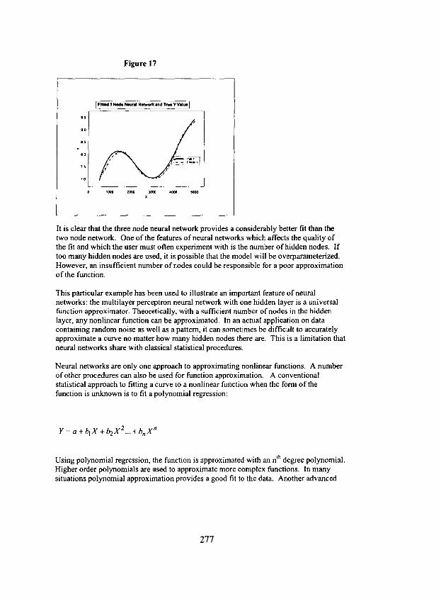
Figure 17
F l l l m d 3 N o d e N e u c d ~ d T ~ e Y V d ~ ]
.¢
I o
e s
>
e o
7 5
7o
x
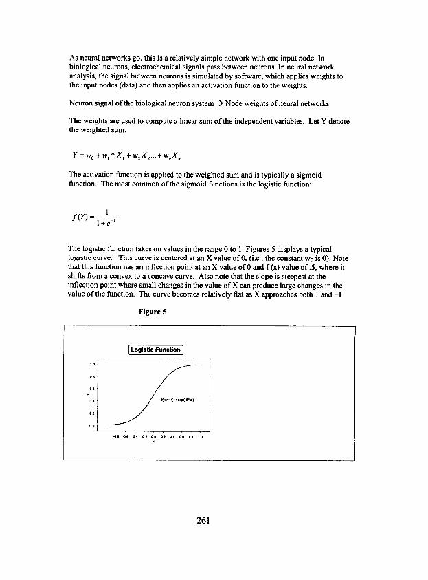
It is clear that the three node neural network provides a considerably better fit than the two node network. One of the features of neural networks which affects the quality of the fit and which the user must often experiment with is the number of hidden nodes. If too many hidden nodes are used, it is possible that the model will be overparameterized. However, an insufficient number of nodes could be responsible for a poor approximation of the function.
This particular example has been used to illustrate an important feature of neural networks: the multilayer perceptron neural network with one hidden layer is a universal function approximator. Theoretically, with a sufficient number of nodes in the hidden layer, any nonlinear function can be approximated. In an actual application on data containing random noise as well as a pattern, it can sometimes be difficult to accurately approximate a curve no matter how many hidden nodes there are. This is a limitation that neural networks share with classical statistical procedures.
Neural networks are only one approach to approximating nonlinear functions. A number of other procedures can also be used for function approximation. A conventional statistical approach to fitting a curve to a nonlinear function when the form of the function is unknown is to fit a polynomial regression:
Y =a+blX+b2X2 . . .+bnX n
th Using polynomial regression, the function is approximated with an n degree polynomial. Higher order polynomials are used to approximate more complex functions. In many situations polynomial approximation provides a good fit to the data. Another advanced
277

method for approximating nonlinear functions is to fit regression splines. Regression splines fit piecewise polynomials to the data. The fitted polynomials are constrained to have second derivatives at each breakpoint; hence a smooth curve is produced. Regression splines are an example ofcontemporary data mining tools and will not be discussed further in this paper. Another function approximator that actuaries have some familiarty with is the Fourier transform which uses combinations of sine and cosine functions to approximate curves. Among actuaries, their use has been primarily to approximate aggregate loss distributions. Heckman and Meyers (Heckman and Meyers, 1983) popularized this application.
In this paper, since neural networks are being compared to classical statistical procedures, the use of polynomial regression to approximate the curve will be illustrated. Figure 18 shows the result of fitting a 4 th degree polynomial curve to the data from Example 2, This is the polynomial curve which produced the best fit to the data. It can be concluded from Figure 18 that the polynomial curve produces a good fit to the data. This is not surprising given that using a Taylor series approximation both the sine function and log function can be approximated relatively accurately by a series of polynomials,
Figure 18 allows the comparison of both the Neural Network and Regression fitted values. It can be seen from this graph that both the neural network and regression provide a reasonable fit to the curve.
Figure 18
Neural Network and Regression Fitted Values
72]
I
6 2 0 1000 2000 3000 4000
X
278

While these two models appear to have similar fits to the simulated nonlinear data, the regression slightly outperformed the neural network in goodness of fit tests. The r 2 for the regression was higher for both training (.993 versus .986) and test (.98 versus .94) data.
Correlated Variables and Dimension Reduction
The previous sections discussed how neural networks approximate functions of a variety of shapes and the role the hidden layer plays in the approximation. Another task performed by the hidden layer of neural networks will be discussed in this section: dimension reduction.
Data used for financial analysis in insurance often contains variables that are correlated. An example would be the age of a worker and the worker's average weekly wage, as older workers tend to earn more. Education is another variable which is likely to be correlated with the worker's income. All of these variables will probably influence Workers Compensation indemnity payments. It could be difficult to isolate the effect of the individual variables because of the correlation between the variables. Another example is the economic factors that drive insurance inflation, such as inflation in wages and inflation in the medical care. For instance, analysis of monthly Bureau of Labor Statistics data for hourly wages and the medical care component of the CPI from January of 1994 through May of 2000 suggest these two time series have a (negative) correlation of about .9 (See Figure l 9). Other measures of economic inflation can be expected to show similarly high correlations.
Figure 19
[ $catterplol of MeO=cal C are and ~4ourly Earn,ngs Inflat=on j
~ ' 0 0 4
O03
3 02 . . . . . . . .
0 020 0 025 0 030 0 035 0 040 0 045 HourtyEarnRate
279

Suppose one wanted to combine all the demographic factors related to income level or all the economic factors driving insurance inflation into a single index in order to create a simpler model which captured most of the predictive ability of the individual data series. Reducing many factors to one is referred to as dimension reduction. In classical statistics, two similar techniques for performing dimension reduction are Factor Analysis and Principal Components Analysis. Both of these techniques take a number of correlated variables and reduce them to fewer variables which retain most of the explanatory power of the original variables.
The assumptions underlying Factor Analysis will be covered first. Assume the values on three observed variables are all "caused" by a single factor plus a factor unique to each variable. Also assume that the relationships between the factors and the variables are linear. Such a relationship is diagrammed in Figure 20, where F1 denotes the common factor, U1, U2 and U3 the unique factors and X1, X2 and X3 the variables. The causal factor FI is not observed. Only the variables X1, X2 and X3 are observed. Each of the unique factors is independent of the other unique factors, thus any observed correlations between the variables is strictly a result of their relation to the causal factor F 1.
F i g u r e 2 0
One Factor Model
///•,X 1 " - - UI
j ~
FU" * X 2 , - U2
~ 3 * U3
For instance, assume an unobserved factor, social inflation, is one of the drivers of increases in claims costs. This factor reflects the sentiments of large segments of the population towards defendants in civil litigation and towards insurance companies as intermediaries in liability claims. Although it cannot be observed or measured, some of its effects can be observed. Examples are the change over time in the percentage of claims being litigated, increases in jury awards and perhaps an index of the litigation environment in each state created by a team of lawyers and claims adjusters. In the social
280

sciences it is common to use Factor Analysis to measure social and psychological concepts that cannot be directly observed but which can influence the outcomes of variables that can be directly observed. Sometimes the observed variables are indices or scales obtained from survey questions.
The social inflation scenario might be diagrammed as follows:
Figure 21
Factor Analysis Diagram
/ / / / . j , Litigation Rates ~ - - - U I
Social Inflation J . . . . Size of Jury ~ U2
Faclor ~ Awards
Index of State Litigation ,,-.- -U3 Environment
In scenarios such as this one, values for the observed variables might be used to obtain estimates for the unobserved factor. One feature of the data that is used to estimate the factor is the correlations between the observed variables: If there is a strong relationship between the factor and the variables, the variables will be highly correlated. If the relationship between the factor and only two of the variables is strong, but the relationship with the third variable is weak, then only the two variables will have a high correlation. The highly correlated variables will be more important in estimating the unobserved factor. A result of Factor Analysis is an estimate of the factor (FI) for each of the observations. The F1 obtained for each observation is a linear combination of the values for the three variable for the observation. Since the values for the variables will differ from record to record, so will the values for the estimated factor.
Principal Components Analysis is in many ways similar to Factor Analysis. It assumes that a set of variables can be described by a smaller set of factors which are linear combinations of the variables. The correlation matrix for the variables is used to estimate these factors. However, Principal Components Analysis makes no assumption about a
281

causal relationship between the factors and the variables. It simply tries to find the factors or components which seem to explain most o f the variance in the data, Thus both Factor Analysis and Principal Components Analysis produce a result of the form:
= w~X~ + ~,v,_X:...+ w ) (
where
i is an estimate o f the index or factor being constructed Xi ..X, are the observed variables used to construct the index w~ ..w, are the ~ eights applied to the variables
An example o f creating an index from observed variables is combining observations related to lit igiousness and the legal environment to produce a social inflation index. Another example is combining economic inflationary variables to construct an economic inflation index for a line o f business, a Factor analysis or Principal Components Analysis can be used to do this. Somet imes the values observed on ~ ariabtes are the result o f or "caused" by more than one underlying factor. The Factor Analysis and Principal Components approach can be generalized to find multiple factors or radices, when the obsers'ed variables are the result of more than one unobserved factor
One can then use these indices in further analyses and discard the original variables. Using this approach, the analyst achieves a reduction in the number of variables used to model thc data and can construct a more parsimonious model.
- S .
Factor Analysts ts an example of a more general class o f models known as Latent Variable Models. For instance, observed values on categorical variables may also be the result o f unobserved factors. It would be difficult to use Factor Analysis to estimate the underlying factors because it requires data from continuous variables, thus an alternative procedure is required. While a discussion o f such procedures is beyond lhe scope o f this paper, the procedures do exist.
It is informative to examine the similarities between Factor Analysis and Principal Components Analysis and neural networks. Figure 22 diagrams lhc relationship between input variables, a single unobserved factor and the dependent variable. In the scenario diagrammed, the input variables are used to derive a single predictive index (FI) and the index is used to predict the dependent variable. Figure 23 diagrams the neural network being applied to the same data. Instead o f a factor or index, the neural network has a hidden layer with a single node. The Factor Analysis index is a weighted linear combination o f the input variables, while in the typical MLP ncural network, the hidden layer is a weighted nonlinear combination o f the input variables. The dcpcndent variable is a linear function o f the Factor in the case o f Factor Analysis and Principal Components Analysis and (possibly) a non linear function o f the hidden layer in the case o f the MLP. Thus, both procedures can be viewed as performing dimension reduction. In the casc o f
In fact Maslerson created such indices for the Property and Casualty lines m the 1960s, s Principal Componenls, because it does not have an underlying causal facrm is nol a lalenr variable model
282

neural networks, the hidden layer performs the dimension reduction. Since it is performed using nonlinear functions, it can be applied where nonlinear relationships exist.
Example 3: Dimension reduction Both Factor Analysis and neural networks will be fit to data where the underlying relationship between a set of independent variables and a dependent variable is driven by an underlying unobserved factor. An underlying causal factor, F a c t o r l , is generated from a normal distribution:
F a c t o r l ~ N(1.05,.025)
On average this factor produces a 5% inflation rate. To make this example concrete F a c t o r l will represent the economic factor driving the inflationary results in a line of business, say Workers Compensation. F a c t o r l drives the observed values on three simulated economic variables, Wage Inflation, Medical Inflation and Benefit Level Inflation. Although unrealistic, in order to keep this example simple it was assumed that no factor other than the economic factor contributes to the value of these variables and the relationship of the factors to the variables is approximately linear.
Figure 22
Factor Analysis Result used for Prediction
Input Variables Factor
*y
Dependent Variable
283

Figure 23
Three Layer Neural Network With One Hidden Node
jjJJ 4
Input Hidden Output
Layer Layer Layer
Also, to keep the example simple it was assumed that one economic factor drives Workers Compensation results. A more realistic scenario would separately model the indemnity and medical components of Workers Compensation claim severity. The economic variables are modeled as followsr:
l n ( W a g e l n f l a t i o n ) = .7 * ln( F a c t o r l ) + e
e - N(0,.005)
In( M e d i c a l l n f i a t i o n ) = 1.3 * In( F a c t o r l ) + e
e - N(0,.01)
I n ( B e n e f i t _ l e v e l _ t r e n d ) = .5 * ln( F a c t o r l ) + e
e ~ N(0,.005)
Two hundred fi~y records of the unobserved economic inflation factor and observed inflation variables were simulated. Each record represented one of 50 states for one of 5 years. Thus, in the simulation, inflation varied by state and by year. The annual inflation rate variables were converted into cumulative inflationary measures (or indices). For each state, the cumulative product of that year's factor and that year's observed inflation
6 Note that the according to Taylor's theorem the natural log of a variable whose value is close to one is approximately equal to 1 minus the vartable's value, i.e., ln(l+x) ~ x. Thus, the economic variables are, to a close approximatton, linear functions of the factor.
284

measures (the random observed variables) were computed. For example the cumulative unobserved economic factor is computed as:
t C u m f a c t o r l t = [1 F a c t o r l k
k=l
A base severity, intended to represent the average severity over all claims for the line of business for each state for each of the 5 years was generated from a lognormal distribution. 7 To incorporate inflation into the simulation, the severity for a given state for a given year was computed as the product of the simulated base severity and the cumulative value for the simulated (unobserved) inflation factor for its state. Thus, in this simplified scenario, only one factor, an economic factor is responsible for the variation over time and between states in average severity. The parameters for these variables were selected to make a solution using Factor Analysis or Principal Components Analysis straightforward and are not based on an analysis of real insurance data. This data therefore had significantly less variance than would be observed in actual insurance data.
Note that the correlations between ihe variables is very" high. All correlations between the variables are at least .9. This means that the problem of multicollineariy exists in this data set. That is, each variable is nearly identical to the others, adjusting for a constant multiplier, so typical regression procedures have difficulty estimating the parameters of the relationship between the independent variables and severity. Dimension reduction methods such as Factor Analysis and Principal Components Analysis address this problem by reducing the three inflation variables to one, the estimated factor or index.
Factor Analysis was performed on variables that were standardized. Most Factor Analysis software standardizes the variables used in the analysis by subtracting the mean and dividing by the standard deviation of each series. The coefficients linking the variables to the factor are called loadings. That is:
Xl = bt Factor1 X2 = b2 Factorl X3 = b3 Factorl
Where Xl , X2 and X3 are the three observed variables, Factorl is the single underlying factor and b~, b2 and b3 are the Ioadings.
In the case of Factor Analysis the Ioadings are the coefficients linking a standardized factor to the standardized dependent variables, not the variables in their original scale. Also, when there is only one factor, the loadings also represent the estimated correlations between the factor and each variable. The loadings produced by the Factor Analysis procedure are shown in Table 8.
7 This distribution will have an average of 5,000 the fwst year (after application of the inflationary factor for year I). Also In(Severity) ~ N(8.47,.05)
285

Table 8 Variable Loading Weights Wage Inflation Index .985 .395 Medical Inflation Index .988 .498 Benefit Level Inflation Index .947 .113
Table 8 indicates that all the variables have a high loading on the factor, and thus all are likely to be important in the estimation of an economic index. An index value was estimated for each record using a weighted sum of the three economic variables. The weights used by the Factor Analysis procedure to compute the index are shown in Table 8. Note that these weights (within rounding error) sum to 1. The new index was then used as a dependent variable to predict each state's severity for each year. The regression model was of the form:
Index =.395 (Wage Inflation)+.498(Medical Inflation)+. 113(Benefit Level Inflation)
S e v e r i t y = a + b * I n d e x + e
where
S e v e r i t y is the simulated severity I n d e x is the estimated inflation Index from the Factor Analysis procedure e is a random error term
The results of the regression will be discussed below where they are compared to those of the neural network.
The simple neural network diagramed in Figure 23 with three inputs and one hidden node was used to predict a severity for each state and year. Figure 24 displays the relationship between the output of the hidden layer and each of the predictor variables. The hidden node has a linear relationship with each of the independent variables, but is negatively correlated with each of the variables. The relationship between the neural network predicted value and the independent variables is shown in Figure 25. This relationship is linear and positively sloped. The relationship between the unobserved inflation factor driving the observed variables and the predicted values is shown in Figure 26. This relationship is positively sloped and nearly linear. Thus, the neural network has produced a curve which is approximately the same form as the "true" underlying relationship.
286

Figure 24
Plot of Predictor Variables vs Hidden Node ]
1.6
12
16
12
BenRa~b~HiddefuNode
MedC PI by Hiaden Node
~ H~da~N~de . . . .
1.6
1.2
00 0.2 0.4 0 6 0 8
HiddenNode
287

F i g u r e 25
I Predictor Variable vs Neural Network Predicted I
1.6
1.2
15ev, Rat I by Neur~Netw~kPred~t~
~ c ~ ~ ~*~o*Pr,O~.~ . . . . . ~_~ ; 1 6 i
~ 12
1 6
1.2
5000 5600 6000 6500 NeuralNetwoll~Predicted
F i g u r e 26
7200
i 52'00
~ .
1 0 11 12 1.3 1 4 Inflation FaCtor
288

Intervretin~ the Neural Network Model With Factor Analysis, a tool is provided for assessing the influence of a variable on a Factor and therefore on the final predicted value. The tool is the factor Ioadings which show the strength of the relationship between the observed variable and the underlying factor. The Ioadings can be used to rank each variable's importance. In addition, the weights used to construct the index s reveal the relationship between the independent variables and the predicted value (in this case the predicted value for severity).
Because of the more complicated functions involved in neural network analysis, interpretation of the variables is more challenging. One approach (Potts, 1999) is to examine the weight connecting the input variables to the hidden layer. Those which are closest to zero are least important. A variable is deemed unimportant only ifaU of these connections are near zero. Table 9 displays the values for the weights connecting the input layer to the hidden layer. Using this procedure, no variable in this example would be deemed "unimportant". This procedure is typically used to eliminate variables from a model, not to quantify their impact on the outcome. While it was observed above that application of these weights resulted in a network that has an approximate linear relationship with the predictor variables, the weights are relatively uninformative for determining the influence of the variables on the fitted values.
Table 9: Factor Example Parameters Wo Wl W2 W3 2.549 -2.802 -3.010 0.662
Another approach to assessing the predictor variables' importance is to compute a sensitivity for each variable (Potts, 1999). The sensitivity is a measure of how much the predicted value's error increases when the variables are excluded from the model one at a time. However, instead of actually excluding variables, they are fixed at a constant value. The sensitivity is computed as follows:
1. Hold one of the variables constant; say at its mean or median value. 2. Apply the fitted neural network to the data with the selected variable held
constant. 3. Compute the squared errors for each observation produced by these modified
fitted values. 4. Compute the average of the squared errors and compare ~t to the average squared
error of the full model. 5. Repeat this procedure for each variable used by the neural network. The
sensitivity is the percentage reduction in the error of the full model, compared to the model excluding the variable in question.
6. If desired, the variables can be ranked based on their sensitivities.
s This would be computed as the product of each variable's weight on the factor limes the coefficient of the factor in a linear regression on the dependent variable (.85 in this example).
289
Since the same set of parameters is used to compute the sensitivities, this procedure does not require the user to refit the model each time a variable's importance is being evaluated, The following table presents the sensitivities of the neural network model fitted to the factor data.
Table 10 Sensitivities of Variables in Factor Example Benefit Level 23.6% Medical Inflation 33.1% Wage Inflation 6.0%
According to the sensitivities, Medical Inflation is the most important variable followed by Benefit Level and Wage Inflation is the least important. This contrasts with the importance rankings of Benefit Level and Wage Inflation in the Factor Analysis, where Wage Inflation was a more important variable than Benefit Level. Note that these are the sensitivities for the particular neural network fit. A different initial starting point for the network or a different number of hidden nodes could result in a model with different sensitivities.
Figure 27 shows the actual and fitted values for the neural network and Factor Analysis predicted models. This figure displays the fitted values compared to actual randomly generated severities (on the left) and to "true" expected severities on the right. The x-axis of the graph is the "true" cumulative inflation factor, as the severities arc a linear
Figure 27
7000
6 0 0 0
5000
Neural Network and Factor Predicted Values . . . . . . . . . . . . [ . . . . . .
700O
l . j 65oo
J o I 60 0 i
SO00
4000 . . . . . . . . . 1 0 1 2 ' ) 4
Cure ulalivQ Factor
N~e~ r~lN et ~o;kP re~ict~d [ ,4 Factor Predlcled
4500 . . . . . .
1 0 1 2 1 4
eumu[atqve Factor
290

function of the factor. However, it should be noted that when working with real data, information on an unobserved variable would not be available.
The predicted neural network values appear to be more jagged than the Factor Analysis predicted values. This jaggedness may reflect a weakness of neural networks: over fitting. Sometimes neural networks do not generalize as well as classical linear models, and fit some of the noise or randomness in the data rather than the actual patterns. Looking at the graph on the right showing both predicted values as well as the "true" value, the Factor Analysis model appears to be a better fit as it has less dispersion around the "true" value. Although the neural network fit an approximately linear model to the data, the Factor Analysis model performed better on the data used in this example. The Factor Analysis model explained 73% of the variance in the training data compared to 71% explained by the neural network model and 45% of the variance in the test data compared to 32% for the neural network. Since the relationships between the independent and dependent variables in this example are approximately linear, this is another instance of a situation where a classical linear model would be preferred over a more complicated neural network procedure.
Interactions
Another common feature of data which complicates the statistical analysis is interactions. An interaction occurs when the impact of two variables is more or less than the sum of their independent impacts. For instance, in private passenger automobile insurance, the driver's age may interact with territory in predicting accident frequencies. When this happens, youthful drivers have a higher accident frequency in some territories than that given by multiplying the age and territory relativities. In other territories it is lower. An example of this is illustrated in Figure 28, which shows hypothetical c u r v e s 9 of expected or "true"(not actual) accident frequencies by age for each of four territories.
The graph makes it evident that when interactions are present, the slope of the curve relating the dependent variable (accident frequency) to an independent variable varies based on the values of a third variable (territory). It can be seen from the figure that younger drivers have a higher frequency of accidents in territories 2 and 3 than in territories 1 and 4. It can also be seen that in territory 4, accident frequency is not related to age and the shape and slope of the curve is significantly different in Territory 1 compared to territories 2 and 3.
9 The curves are based on s~nulated data. However data from the Baxter (Venebles and Ripley) automobile claims database was used to develop parameters for the simulation.
291

Figure 28
=~O3
0 1
T ~ . a r y 3
Tln'ilary 1 T ~ 2 _ _
: , , , , r ,
U
0.3
0 1
17 22.5 3 2 5 47,5 ~ . 5 7 7 5 17 22.5 3 2 5 4 7 5 6 2 5 7 7 5
292

As a result of interactions, the true expected frequency cannot be accurately estimated by the simple product of the territory relativity times the age relativity. The interaction of the two terms, age and territory, must be taken into account. In linear regression, interactions are estimated by adding an interaction term to the regression. For a regression in which the classification relativities are additive:
Yta = B0 + (Bt * Territory) + (B=*Age) + (B= * Territory * Age)
Vl/here:
Y= = is either a pure premium or loss ratio for territory t and age a B0 = the regression constant Bt, Ba and Bat a re coefficients of the Territory, Age and the Age, Territory interaction
It is assumed in the regression model above that Territory enters the regression as a categorical variable. That is, if there are N territories, N-1 dummy variables are created which take on values of either I or 0, denoting whether an observation is or is not from each of the territories. One territory is selected as the base territory, and a dummy variable is not created for it. The value for the coefficient B0 contains the estimate of the impact of the base territory on the dependent variable. More complete notation for the regression with the dummy variables is:
Yt~ = B0 + Btl*T1 + Bt2*T2 + Bt3 * T3 +B=*Age + Batl* Tl*Age+ Bat2* T2*Age+ Bat3* T3*Age
where TI, T2 and T3 are the dummy variables with values of either I or 0 described above and Btl - Bt3 are the coefficients of the dummy variables and Bail- Bat3* are coefficients of the age and territory interaction terms. Note that most major statistical packages handle the details of converting categorical variables to a series of dummy variables.
The interaction term represents the product of the territory dummy variables and age. Using interaction terms allows the slope of the fitted line to vary by territory. A similar formula to that above applies if the class relativities are multiplicative rather than additive; however, the regression would be modeled on a log scale:
ln(Y~ )= B*0 + (B*t * Territory) + (B 'a 'Age) + (B'at * Territory * Age)
where B*0, B' t , B*= and B'at are the log scale constant and coefficients of the Territory, Age and Age, Territory interaction.
Examole 3: Interactions To illustrate the application of both neural networks and regression techniques to data where interactions are present 5,000 records were randomly generated. Each record represents a policyholder. Each policyholder has an underlying claim propensity dependent on his/her simulated a g e and territory, including interactions between these
293

two variables. The underlying claim propensity for each age and territory combination was that depicted above in Figure 28. For instance, in territory 4 the claim frequency is a fiat .12. In the other territories the claim frequency is described by a curve. The claim propensity served as the Poisson parameter for claims following the Poisson distribution:
"~'6 x
P(X = x ; 2 ~ ) = x! e a~'
Here k,j is the claim propensity or expected claim frequency for each age, territory combination. The claim propensity parameters were used to generate claims from the Poisson distribution for each o f the 5,000 policyholders.l°
Models for count data The claims prediction procedures described in this section apply models to data with discrete rather than continuous outcomes. A policy can be viewed as having two possible outcomes: a claim occurs or a claim does not occur. We can assign the value 1 to observations with a claim and 0 to observations without a claim. The probability the policy will have a value o f I lies in the range 0 to 1. When modeling such variables, it is useful to use a model where the possible values for the dependent variable lie in this range. One such modeling technique is logistic regression. The target variable is the probability that a given policyholder will have a claim, and this probability is denoted p(x). The model relatingp(x) to the a vector o f independent variables x is:
l n ( i P ; x ) = B o+B~X~+...+B.X. - p
where the quantity ln(p(x)/(l-p(x))) is known as the logit function.
In general, specialized software is required to fit a logistic regression to data, since the logit function is not defined on individual observations when these observations can take on only the values 0 or 1. The modeling techniques work from the likelihood functions, where the likelihood function for a single observation is:
/ ( x , ) = p ( x ; ) " , (1 - p ( x , ) '- "~ )
I p(x;) -
Where xil. . .xi, are the independent variables for observation i, y, is the response (either 0 or !) and BI..B, are the coefficients o f the independent variables in the logistic regression. This logistic function is similar to the activation function used by neural networks. However, the use o f the logistic function in logistic regression is very different from its use in neural networks. In logistic regression, a transform, the logit transform, is
m The overall distribution of drivers by age used in the simulation was based on fitting a curve to infoznmtion from the US Department of Transportation web site.
294

applied to a target variable modeling it directly as a function of predictor variables. After parameters have been fit, the function can be inverted to produce fitted frequencies. The logistic functions in neural networks have no such straightforward interpretation. Numerical techniques are required to fit logistic regression when the maximum likelihood technique is used. Hosmer and Lemshow (Hosmer and Lemshow, 1989) provide a clear but detailed description of the maximum likelihood method for fitting logistic regression. Despite the more complicated methods required for fitting the model, in many other ways, logistic regression acts like ordinary least squares regression, albeit, one where the response variable is binary. In particular, the logit of the response variable is a linear function of the independent variables. In addition interaction terms, polynomial terms and transforms of the independent variables can be used in the model.
A simple approach to performing logistic regression (Hosmer and Lemshow, 1989), and the one which will be used for this paper, is to apply a weighted regression technique to aggregated data. This is done as follows:
1. Group the policyholder's into age groups such as 16 to 20, 21 to 25, etc. 2. Aggregate the claim counts and exposure counts (here the exposure is
policyholders) by age group and territory. 3. Compute the frequency for each age and territory combination by dividing the
number of claims by the number of policyholders. 4. Apply the logit transform to the frequencies (for logistic regression). That is
compute Iog(p/(l-p)) where p is the claim frequency or propensity. It may be necessary to add a very small quantity to the frequencies before the transform is computed, because some of the cells may have a frequency of 0.
5. Compute a value for driver age in each cell. The age data has been grouped and a value representative of driver ages in the cell is needed as an independent variable in the modeling. Candidates are the mean and median ages in the cell. The simplest approach is to use the midpoint of the age interval.
6. The policyholder count in each cell will be used as the weight in the regression. This has the effect of cau~,ng the regression to behave as if the number of observations for e: ~h cell equals the number of policyholders.
One of the advantages of using the aggregated data is that some observations have more than one claim. That is, the observations on individual records are not strictly binary, since values of 2 claims and even 3 claims sometimes occur. More complicated methods such as multinomial logistic regression N can be used to model discrete variables with more than 2 categories. When the data is aggregated, all the observations of the dependent variable are still in the range 0 to 1 and the Iogit transform still is appropriate for such data. Applying the logit transform to the aggregated data avoids the need for a more complicated approach. No transform was applied to the data to which the neural network was applied, i.e., the dependent variable was the observed frequencies. The result of aggregating the simulated data is displayed in Figure 29.
H A Poisson regression using Generalized Linear Models could also be used.
295

Figure 29
==
02
Plot of Simulated Frequencies I
Temto~: 3 i Temtoqf 4 - - t 05
i
02 C ̧ ~ i
Temlo~: 1 [ Ternto~ 2 ~ . . . . . . .
17 225 325 475 625 775 17 225 325 475 625 775 Age
Neural Network Results A five node neural network was fit to the data. The weights between the input and hidden layers are displayed in Table 11. If we examine the weights between the input and the hidden nodes, no variables seem insignificant, but it is hard to determine the impact that each variable is having on the result. Note that weights are not produced for Territory 4. This is the base territory in the neural network procedure and its parameters are incorporated into we, the constant.
Table 11 : Weights to Hidden Layer Node! N0(Constant) Neight(Age) Weight(Territory 1 ) Neight(Territory 21 Neight(Territory 3)
t -0.01 0.18 -0.02 -0.OE 0.09 0.3. = -0.01 -1,06 -0.73 -0.10
-0.3( 0.21 -0.07 -0.8; 0.46 4 -(3.0' 0.19 -0,01 -0.0~ 0.09 5 0.56 -0.08 -0.90 -1.1( -0,98
Interpreting the neural network is more complicated than interpreting a typical regression. In the previous section, it was shown that each variable's importance could be measured by a sensitivity. Looking at the sensitivities in Table 12, it is clear that both age and territory have a significant impact on the result. The magnitude of their effects seems to I~ roughly oqual
296

Table 12: Sensitivity of Variables in Interaction Example Variable Sensitivity Age 24% Territory 23%
Neither the weights nor the sensitivities help reveal the form of the fitted function. However graphical techniques can be used to visualize the function fitted by the neural network. Since interactions are of interest, a panel graph showing the relationship between age and frequency for each territory can be revealing. A panel graph has panels displaying the plot of the dependent variable versus an independent variable for each value of a third variable, or for a selected range of values of a third variable. (Examples of panel graphs have already been used in this paper in this section, to help visualize interactions). This approach to visualizing the functional form of the fitted curve can be useful when only a small number of variables are involved. Figure 30 displays the neural network predicted values by age for each territory. The fitted curve for territories 2 and 3 are a little different, even though the "true" curves are the same. The curve for territory 4 is relatively fiat, although it has a slight upward slope.
Figure 30
I Neural N*tWork Prod6cled by Age snd TerJ~to~
~ 0 2 0
17 225 325 475 625 775 17 225 325 475 625 775 Age
0 20
OlO
Re~ression fit Table 13 presents the fitted coefficients for the logistic regression. Interpreting these coefficients is more difficult than interpreting those of a linear regression, since the logit represents the log of the odds ratio (p/(1-p)), wherep represents the underlying true claim frequency. Note that as the coefficients of the Iogit of frequency become more positive, the frequencies themselves become more positive. Hence, variables with positive
297

coefficients are positively related to the dependent variable and cocfficicnts with negative signs are negatively related to the dependent variable.
Table 13: Results of Regression Fit Variable Coefficient Significance Intercept -1.749 0 Age -0.038 0.339 Territory 1 -0.322 0.362 Territory 2 -0.201 0.451 Territory 3 -0.536 0.051 Age'Territory 1 0.067 0.112 Age*Territory 2 0031 0.321 Age*Territory 3 0.051 0.079
Figure 31 displays the frequencies fitted by the logistic regression. As with neural networks graph are useful for visualizing the function fitted by a logistic regression. A noticeable departure from the underlying values can be seen in the results for Territory 4. The fitted curve is upward sloping for Territory 4, rather than nat as the true values are.
Figure 31
~020
Regression Predicted by Age and Territory
i 0 2 0
O 05
17 21 2 5 5 3 2 5 4 2 5 5 2 5 6 2 5 7 2 5 8 2 5 17 21 2 5 5 3 2 5 4 2 5 5 2 5 6 2 5 7 2 5 e 2 5 a ~
298

I rrab'a 14 I esults of Fits: Mean squared error
[Training Data~est Data eural Network| 0.005t 0,014 egression l 0.007] 0.016
In this example the neural network had a better performance than the regression. Table 14 displays the mean square errors for the training and test data for the neural network and the logistic regression. Overall, the neural network had a better fit to the data and did a better job of capturing the interaction between Age and Territory. The fitted neural network model explained 30 % of the variance in the training data versus 15% for the regression. It should be noted that neither technique fit the "true" curve as closely as the curves in previous examples were fit. This is a result of the noise in the data. As can be seen from Figure 29, the data is very noisy, i.e., there is a lot of randomness in the data relative to the pattern. The noise in the data obscures the pattern, and statistical techniques applied to the data, whether neural networks or regression will have errors in their estimated parameters.
Example 5: An Example with Messy Data
The examples used thus far were kept simple, in order to illustrate key concepts about how neural networks work. This example is intended to be closer to the typical situation where data is messy. The data in this example will have nonlinearities, interactions, correlated variables as well as missing observations.
To keep the example realistic, many of the parameters of the simulated data were based on information in publicly available databases and the published literature. A random sample of 5,000 claims was simulated. The sample represents 6 years of claims history. (A multiyear period was chosen, so that inflation could be incorporated into the example). Each claim represents a personal automobile claim severity developed to ultimate 12. As an alternative to using claims developed to ultimate, an analyst might use a database of claims which are all at the same development age. Random claim values were generated from a lognormal distribution. The scale parameter, p., of the lognormal, (which is the mean of the logged variables) varied with the characteristics of the claim. The claim characteristics in the simulation were generated by eight variables. The variables are summarized in Table 15. The la parameter itself has a probability distribution. A graph of the distribution of the parameter in the simulated sample is shown in Figure 32. The parameter had a standard deviation of approximately .38. The objective of the analysis is to distinguish high severity policyholders from low severity
12 The analyst may want to use neural network or other data mining techniques to develop the data.
299

Figure32
1.2
0.8
0.4
0.0 6.50 6.75 700 725 7.50 7.75 8.00 825 850 8 75 900
MU
J Distribution of Mu ]
policyholders. This translates into an estimate ofp. which is as close to the "true" p as possible.
Table 15 below lists the eight predictor variable used to generate the data in this example. These variables are not intended to serve as an exhaustive list of predictor variables for the personal automobile line. Rather they are examples of the kinds of variables one could incorporate into a data mining exercise. A ninth variable (labeled Bogus) has no causal relationship to average severity. It is included as a noise variable to test the statistical procedures in their effectiveness at using the data. An effective prediction model should be able to distinguish between meaningful variables and variables which have no relationship to the dependent variable. Note that in the analysis of the data, two of the variables used to create the data are unavailable to the analyst as they represent unobserved variables (the Auto BI and Auto PD underlying inflation factors). Instead, six inflation indices which are correlated with the unobserved Factors are ayailable to the analyst for modeling. Some features of the variables are listed below.
300

Number of Categories
~,ge of Driver Territory ~ge of Car 3ar Type 3redit Rating IAuto BI Inflation Factor
Auto PD and Phys Dam Inflation Factor
Law Change Bogus
Variable Type
Continuous Categorical Continuous Categorical Continuous Continuous
Continuous
Categorical Continuous
45
No
Missing Data
No No Yes No Yes No
No No
Table 15 Variable
Note that some of the data is missing for two of the variables. Also note that a law change was enacted in the middle of the experience period which lowered expected claim severity values by 20%. A more detailed description of the variables is provided in Appendix 2.
Neural Network Analysis of Simulated Dalo The dependent variable for the model fitting was the log of severity. A general rule in statistics is that variables which show significant skewness should be transformed to approximate normality before fitting is done. The log transform is a common transform for accomplishing this. In general, Property and Casualty severities are positively skewed. The data in this example have a skewness of 6.43, a relatively high skewness. Figure 33, a graph of the distribution of the log of severity indicates that approximate normality is attained after the data is logged.
Figure 33
O*¢,nbulo~ ot ~ol(S*~h~v)
. i , 311771O o GOtGO 1 114$o 1o/ooo7 IZ ~ l l l N
mo(so~s*~y)
301

The data was separated into a training database of 4,000 claims and a test database of 1,000 claims. A neural network with 7 nodes in the hidden layer was run on the 4,000 claims in the training database. As will be discussed later, this network was larger than the final fitted network. This network was used to rank variables in importance and eliminate some variables. Because the amount of variance explained by the model is relatively small (8%), the sensitivities were also small. Table 16 displays the results of the sensitivity test for each of the variables. These rankings were used initially to eliminate two variables from the model: Bogus, and the dummy variable for car age missing. Subsequent testing of the model resulted in dropping other variables. Despite their low sensitivities, the inflation variables were not removed. The low sensitivities were probably a result of the high correlations of the variables with each other. In addition, it was deemed necessary to include a measure of inflation in the model. Since the neural network's hidden layer performs dimension reduction on the inflation variables, in a manner analogous to Factor or Principal Components Analysis, it seemed appropriate to retain these variables.
Table 16: Sensitivities of Neural Network Variable Sensitivity Rank Car age 9.0 1 Age 5.3 2 Car type 3.0 3 Law Change 2.2 4 Credit category 2.2 5 Territory 2.0 6 Credit score 1.0 7 Medical Inflation 0,5 8 Car age missing 0.4 9 Hospital Inflation 0.1 10 Wage Inflation 0,0 11 Other Services Inflation 0.0 12 Bogus 0.O 13 Parts Inflation 0.0 14 Body Inflation 0.0 15
One danger that is always present with neural network models is overtltting. As more hidden layers nodes are added to the model, the fit to the data improves and the r 2 of the model increases. However, the model may simply be fitting the features of the training data, therefore its results may not generalize well to a new database. A rule of thumb for the number of intermediate nodes to include in a neural network is to use one half of the number of variables in the model. After eliminating 2 of the variables, 13 variables remained in the model. The rule of thumb would indicate that 6 or 7 nodes should be used. The test data was used to determine how well networks of various sizes performed when presented with new data. Neural networks were fit with 3, 4, 5, 6 and 7 hidden nodes. The fitted model was then used to predict values of claims in the test data. Application of the fitted model to the test data indicated that a 4 node neural network
302

provided the best model. (It produced the highest r e in the test data). The test data was also used to eliminate additional variables from the model. In applying the model to the test data it was found thai dropping the territory and credit variables improved the fit.
Goodness of Fit The fitted model had an r 2 of 5%. This is a low re but not out of line with what one would expect with the highly random data in this example. The "true" la (true expected log (severity)) has a variance equal to 10% of the variance of the log of severity. Thus, if one had perfect knowledge of ~t, one could predict individual log(severities) with only 10% accuracy. However, if one had perfect knowledge of the true mean value for severity for each policyholder, along with knowledge of the true mean frequency for each policyholder, one could charge the appropriate rate for the policy, given the particular characteristics of the policyholder. In the aggregate, with a large number of policyholders, the insurance company's actual experience should come close to the experience predicted from the expected severities and frequencies.
With simulated data, the "true" la for each record is known. Thus, the model's accuracy in predicting the true parameter can be assessed. Figure 34 plots the relationship between ~t and the predicted values (for the log of severity). It can be seen that as the predicted value increases, p. increases. The correlation between the predicted values and the parameter mu is .7.
i : I
Figure 34
Scatterplot of Neural Network Predicted vs Mu
7 ~ 8 0 8S
As a further test of the model fit, the test data was divided into quartiles and the average severity was computed for each quartile. A graph of the result is presented in Figure 35. This graph shows that the model is effective in discriminating high and low severity claims. One would expect an even better ability to discriminate high severity from low severity observations with a larger sample. This is supported by Figure 36 which displays the plot of"true" expected severities for each of the quartiles versus the neural
303

network predicted values. This graph indicated that the neural network is effective in classifying claims into severity categories. These results suggest that neural networks could be used to identify the more profitable insureds (or less profitable insureds) as part of the underwriting process.
Figure 35
I
5°°° 1 77
j ~ j ~
i f j J /
7 9 81 83 NN Pr edic~,ed
Figure 36
l ob( of Neural Network Pn~hcted Log(Seventy) ~/s True Expected Sevetly I
80OO
~7coo
t ~ s(x~o
77 7 9 81 8 3
lnteroretino Neural Networks Revisited: Visualizing Neural Network Results
304

In the previous example some simple graphs were used to visualize the form of the fitted neural network function. Visualizing the nature of the relationships between dependent and independent variables is more difficult when a number of variables are incorporated into the model. For instance, Figure 37 displays the relationship between the neural network predicted value and the driver's age. It is difficult to discern the relationship between age and the network predicted value from this graph. One reason is that the predicted value at a given age is the result of many other predictor variables as well as age. Thus, there is a great deal of dispersion of predicted values at any given age due to these other variables, disguising the fitted relationship between age and the dependent variable.
Figure 37
~eo / "fl
20 40 GO 80
Researchers on neural networks have been exploring methods for understanding the function fit by a neural network. Recently, a procedure for visualizing neural network fitted functions was published by Plate, Bert and Band (Plate et ai., 2000). The procedure is one approach to understanding the relationships being modeled by a neural network. Plate et al. describe their plots as Generalized Additive Model style plots. Rather than attempting to describe Generalized Additive Models, a technique for producing the plots is simply presented below. (Both Venables and Ripley and Plate et al. provide descriptions of Generalized Additive Models). The procedure is implemented as follows:
I .
2.
Set all the variables except the one being visualized to a constant value. Means and medians are logical choices for the constants. Apply the neural network function to this dataset to produce a predicted value for each value of the independent variable• Alternatively, one could choose to apply the neural network to a range of values for the independent variable selected to represent a reasonable set of values of the variable. The other variables remain at the selected constant values.
305

3. 4.
Plot the relationship between the neural network predicted value and the variable. Plate el al. recommend scaling all the variables onto a common scale, such as 0 to 1. This is the scale of the inputs and outputs of the logistic functions in the neural network. In this paper, variables remain in their original scale.
The result of applying the above procedure is a plot of the relationship between the dependent variable and one of the independent variable. Multiple applications of this procedure to different variables in the model provides the analyst with a tool for understanding the functional form of the relationships between the independent and dependent variables.
The visualization method was applied to the data with all variablcs set to constants except for driver age. The result is shown in Figure 38. From this graph we can conclude that the fitted function declines with driver age. Figure 39 shows a similar plot for car age. This function declines with car age, but then increases at older ages.
Figure 38
=
o
Visuahzation P~ot of Predicted log(Severity) vs Age
306

Figure 39
Visualization Plot of Predicted log(Severity) vs car age
• - <o
tO I<
¢ ;
~ J D " q l 2 4 0 , :
0 5 10 1 S 20
car age
Suppose we wanted to visualize the relationship between a predictor variable which takes on discrete values and the dependent variable. For instance, suppose we wanted to know the impact of the law change. We can create fitted values for visualizing as described above but instead of producing a scatterplot, we can produce a bar chart. Figure 40 displays such a graph. On this graph, the midpoint for claims subject to the law change (a value of I on the graph) is about .2 units below the midpoint of claims not subject to the law change. This suggests that the neural network estimates the law effect at about 20% because a .2 impact on a log scale corresponds approximately to a multiplicative factor of 1.2, or .8 in the case of a negative effect (Actually, the effect when converted from the log scale is about 22%). The estimate is therefore close to the "true" impact of the law change, which is a 20% reduction in claim severity.
307
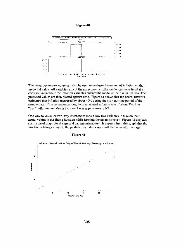
Figure 40
2 0 0 0
1 5 0 0
1 0 0 0
SO0
o
[ W t u l l * l a t , o n P~ol o~ p r l a t ¢ l e a ~1 L l w c LoBISoVerlty) ~ lnge
[ L , . , eo
7 70 7 80 7 90 8 00 e 10 8 20 8 30 $ 40 8 50 Predicted
I 20OO
I~oo
1ooo
soo
o
The visualization procedure can also be used to evaluate the impact of inflation on the predicted value. All variables except the six economic inflation factors were fixed at a constant value while the inflation variables entered the model at their actual values. The predicted values are then plotted against time. Figure 41 shows that the neural network estimated that inflation increased by about 40% during the six year time period of the sample data. This corresponds roughly to an annual inflation rate of about 7%. The "true" inflation underlying the model was approximately 6%.
One way to visualize two-way interactions is to allow two variables to take on their actual values in the fitting function while keeping the others constant. Figure 42 displays such a panel graph for the age and car age interaction. It appears from this graph that the function relating car age to the predicted variable varies with the value of driver age.
Figure 41
I n f l a t i o n V i s u a l i z a t i o n _Pl~t o f P r e d i c t e d I o g ( S e v e r i t y ~ vs. T i m e
,5 10 15 20
Quarters of • Year
308

Figure 42
~ , i
, e ~
o io 2 ~ r ~
Rem'ession Model A regression model was fit to the data. The dependent variable was the log o f severity. Like neural networks, regression models can be subject to overfitting. The more variables in the model, the better the fit to the training data. However, if the model is overfit it will not generalize well and will give a poor fit on new data. Stepwise regression is an established procedure for selecting variables for a regression model. It tests the variables to find the one that produces the best r z. This is added to the model. It continues cycling through the variables, testing variables and adding a variable each cycle to the model until no more significant variables can be found. Significance is usually determined by performing an F-test on the difference in the r 2 of the model without a given variable and then with the variable.
Stepwise regression was used to select variables to incorporate into the model. Then a regression on those variables was run. The variables selected were driver age, car age, a dummy variable for the law change and the hospital inflation factor. Note that the hospital inflation factor had a very high correlation with both underlying inflation factors (even though the factors were generated to be independent o f each other Z 3). Thus, using just the one variable seems to adequately approximate inflation. On average, the increase in the hospital inflation index was 4.6%. Since a factor o f 1.15 (see Table 17) was applied to the hospital inflation factor, inflation was estimated by the regression to be a little over 5% per year, The regression model estimated the impact o f the law change as a reduction of .3 on the log scale or about 35% as opposed to the estimate 0fabout 22% for the neural network. Thus, the neural network overestimated inflation a little, while the regression model underestimated it a little. The neural network estimate o f the law
~3 This may be a result of using a random walk procedure to generate both variable. Using random walk models, the variables simulated have high correlations with prior values in the series.
309

change effect was close to the "true" value, while the regression overestimated the magnitude of the effect.
The regression found a negative relationship between driver age and severity and between car age and severity. An interaction coefficient between age and car age was also estimated to be negative. The results correspond with the overall direction of the "true" relationships. The results of the final regression are presented in Table 17.
The fitted regression had a somewhat lower r 2 than the neural network model. However, on some goodness of fit measures, the regression performance was close to that of the neural network. The regression predicted values had a .65 correlation with It. versus .70 for the neural network. As seen in Figures 43 and 44, the regression was also able to discriminate high severity from low severity claims with the test data. Note that neither model found the Bogus variable to be significant. Also, neither model used all the variables that were actually used to generate the data, such as territory or credit information. Neither technique could distinguish the effect of these variables from the overall background noise in the data.
Table 17: Regression Results Variable Coefficient Significance Intercept 7.210 0 Age -0.001 0.448 car age -0,024 0.203 Law -0.306 0.0001 Hospital Inf 1.1 0,0059 Age*car age -0.001 0.0195 R 2 = .039
Figure 43
70o0
7 ~
/
/ / /
i /
• / J / / 7
77 79 81 1~3 R m ~ fitted Io~(Se~mly)
310

F i g u r e 4 4
J
i r r 79 a l e3
Re~e,~en ~ee~
Usin~ the model in prediction To estimate severities, the fitted log severities must be transformed back to their original scale. This is generally accomplished by applying the exponential function to the values predicted by the model. If the data is approximately Iognormally distributed, as in this example, a simple exponential transform will understate the true value of the predicted severity. The mean o f a lognormal variable is given by:
, z
E ( Y , ) = e . . . . . .
where
E(Y,) is the expected value for the i th observation lai = the mean for i 'h observation on the log scale 2 is the variance of severities on a log scale
Since ~ti and o 2 are unknown, estimates of their values must be used. The predicted value from the neural network or regression is the usual choice for an estimate o f [u.i. The mean square error o f the neural network or regression can be used as an estimate o f o 2 in the formula above. A predicted value was computed for the claims that were used to fit the neural network model. A plot o f the predicted severities versus the "true" expected severities is displayed in Figure 43.
311

Figure 43
!°
o
o
Scatterplot of Expected versus Predicted Severity
0 2000 4 0 0 0 6 0 0 0 8 0 0 0 1 0 0 0 0 1200D
Pced lc led
Applying the models Some of the possible applications of neural networks and other modeling techniques can utilize predictions of claim severity. A company may want to devise an early warning system to screen newly reported claims for those with a high probability of developing into large settlements. A severity model utilizing only information available early in the life of a claim could be used in an early warning system. A fraud detection system could also be based on claim severity. One approach to fraud detection is to produce a severity prediction for each claim. The actual value of the claim is compared to the predicted value. Those with a large positive deviation from the predicted are candidates for further investigation.
However, many of the underwriting applications of modeling and prediction require both a frequency and a severity estimate. A company may wish to prune "bad" risks from its portfolio, pursue "good" risks or actually use models to establish rates. For such applications either the loss ratio or pure premium will be the target variable of interest. There are two approaches to estimating the needed variable: 1 ) One can separately estimate frequency and severity models and combine the estimates of the two models. An illustration of fitting models to frequencies was provided in Example 4 and an example of fitting models to severities was supplied in Example 5. 2) Alternatively, one can estimate a pure premium or loss ratio model directly.
One difficulty of modeling pure premiums or loss ratios is that in some lines of business, such as personal lines, most of the policyholders will have no losses, since the expected frequency is relatively low. It is desirable to transform the data onto a scale that does not allow for negative values. The log transformation accomplishes this. However, since the
312

log is not defined for a value of zero it may be necessary to add a very small constant to the data in order to apply the log transform.
Once a pure premium is computed, it can be converted into a rate by loading for expenses and profit. Alternatively, the pure premium could be ratioed to premium at current rate levels to produce a loss ratio. A decision could be made as to whether the predicted loss ratio is acceptable before underwriting a risk. Alternatively the loss ratio prediction for a company's portfolio of risks for a line of business can be loaded for expenses and profit and the insurance company can determine if a rate increase is needed.
Summarv This paper has gone into some detail in describing neural networks and how they work. The paper has attempted to remove some of the mystery from the neural network "black box". The author has described neural networks as a statistical tool which minimizes the squared deviation between target and fitted values, much like more traditional statistical procedures do. Examples were provided which showed how neural networks 1) are universal function approximators and 2) perform dimension reduction on correlated predictor variables. Classical techniques can be expected to outperform neural network models when data is well behaved and the relationships are linear or variables can be transformed into variables with linear relationships. However neural networks seem to have an advantage over linear models when they are applied to complex nonlinear data. This is an advantage neural networks share with other data mining tools not discussed in detail in this paper. Future research might investigate how neural networks compare to some of these data mining tools.
Note that the paper does not advocate abandoning classical statistical tools, but rather adding a new tool to the actuarial toolkit. Classical regression performed well in many of the examples in this paper. Some classical statistical tools such as Generalized Linear Models have been applied successfully to problems similar to those in this paper. (See Holler et al. for an example).
A disadvantage of neural networks is that they are a "black box". They may outperform classical models in certain situations, but interpreting the result is difficult because the nature of the relationship between dependent and target variables is not usually revealed. Several methods for interpreting the results of neural networks were presented. Methods for visualizing the form of the fitted function were also presented in this paper. Incorporating such procedures into neural network software should help address this limitation.
313

A p p e n d i x 1 : N e u r a l N e t w o r k S o f t w a r e
Neural network software is sold at prices ranging from a couple o f hundred dollars to $100,000 or more. The more expensive prices are generally associated with more comprehensive data mining products, which include neural networks as one of the capabilities offered. Some o f the established vendors o f statistical software such as SPSS and SAS sell the higher end data mining products 14. These products are designed to function on servers and networks and have the capability o f processing huge databases. They also have some o f the bells and whistles useful to the analyst in evaluating the function fit by the neural network, such as a computation o f sensitivities. Both o f these products allow the user to apply a number o f different kinds o f neurat networks, including types o f networks not covered in this paper.
Many o f the less expensive products provide good fits to data when the database is not large. Since the examples in this paper used modestly sized databases, an expensive product with a lot o f horsepower was not required. Two of the less expensive tools were used to fit the models in this paper: a very inexpensive neural network package, Brainmaker, and the S-PLUS neural network function, nnet. The Brainmaker tool has a couple o f handy features. It creates a file that contains all the parameters o f the fitted neural network function for the hidden and output layers. It also has the capability o f producing the values o f the hidden nodes. Both o f these features were helpful for the detailed examination o f neural networks contained in this paper. However, the Brainmaker version employed in this analysis had difficulty filling networks on larger databases l-s, so the S-PLUS nnet function was used for the last example. The S-PLUS rmet function is contained in a library supplied by Venables and Ripley, rather than the vendors o f S-PLUS, but it is included in the basic S-PI,US package. This software also provides the fitted parameters for the hidden and output layers. (However, it does not provide the fitted values for the hidden nodes). Chapter 9 o f Venables and Ripley describes the software and how to use it. (Venables and Ripley, 1999).
The commonly used commercial software for fitting neural networks does not incorporate the visualization technique used for Example 5. Plate has provided an S- PLUS library incorporating his visualization technique (which is similar to, but a little different from, the one used for this paper) in the statlib library, at htto://lib.stat.cmd.edu/S/. The library with the visualization software is named Ploteff.
Numerous other products with which the author o f this paper has no experience are also available for fitting neural networks. Thus, no statement made in this paper should be interpreted as an endorsement o f any particular product.
14 The SPSS dam mining product is called Clementine. lT, e SAS product ~s called the Enterprise Miner. SPSS also sells an inexpensive neural network product, Neural Conncction q~e author has used Neural Connection on moderately sized databases and found it to be effecnve on prediction and classification groblems.
It should be noted that lhe vendors of Brainmaker sell a professional version which probably performs better on large databases.
3 1 4

Appendix 2
This appendix is provided for readers wishing a little more detail on the structure of the data in the Example 5.
The predictor variables are: Driver age: Age of the driver in years Car type: This is intended to represent classifications like compact, midsize, sports utility vehicle and luxury car. There are 4 categories. Car age: Age of the car in years Representative parameters for the Driver age, Car type and Car age and their interactions variables were determined from the Baxter automobile claims database 16 Territory: Intended to represent all the territories for 1 state. There are 45 categories. Reasonable parameters for territory were determined after examining the Texas automobile database used in the Casualty Actuarial Society's ratemaking competition. Credit: A variable called leverage, representing the ratio o f the sum of all revolving debt to the sum of all revolving credit limits was used as an indicator of the creditworthiness of the driver. This is a variable not typically used in ratemaking. However, some recent research has suggested it may be useful in predicting personal lines loss ratios. Monaghan (Monagahan, 2000) shows that credit history has a significant impact on personal automobile and homeowners' loss ratios. Monaghan discussed a number of possible credit indicators, which were useful in predicting loss ratios. The leverage variable was judgmentally selected for this model because it had high predictive accuracy and because parameters could be developed based on information in Monaghan's paper. I fa company had access to its policyholders' credit history, it might wish to develop a separate credit score (perhaps using neural networks) which used the information of a number of credit history variables. Another credit variable was used in addition to the leverage ratio. People with a leverage ratio of 0 were divided into 2 categories, those with very low limits (< $500) and those with higher limits (>=$500). A third category was created for claimants with leverage greater than 0. For the purposes of illustrating this technique, it was assumed that the entire impact of the credit variable is on severity, although this is unlikely in practice.
Automobile Bodily Injury (ABI) inflation factor and Automobile Property Damage and Physical Damage (APD) inflation factor: These factors drive quarterly increases in the bodily injury, property damage and physical damage components of average severity. They are unobserved factors. The ABI factor is correlated with three observed variables: the producer price index for hospitals, the medical services component of the consumer price index and an index of average hourly earnings. The APD factor is correlated with three observed variables: the produce price index for automobile bodies, the producer price index for automobile parts and the other services component of the consumer price index. Bureau of Labor statistics data was reviewed when developing parameters for the factors and for the "observed" variables. The ABI factor was given a 60% weight and the APD factor was given a 40% weight in computing each claim's expected severity.
~6 This database of Automobile claims is available as an example database in S-PLUS. Venables and Ripley supply the S-PLUS data for claim severities in a S-PLUS library. See Venables and Ripley, p.467.
315

Law Change: A change in the law is enacted which causes average severities to decline by 20% after the third year.
Interactions: Table 18 shows the variables with interactions. Three o f the variables have interactions. In addition some o f the interactions are nonlinear (or piecewise linear). An example is the interactions between age and car age. This is a curve that has a negative slope at older car ages and younger driver ages, but is flat for older driver ages and younger car ages. The formula used for generating the interaction between age, car age and car type is provided below (after Table 19). In addition to these interactions, other relationships exist in the data, which affect the mix o f values for the predictor variables in the data. Young drivers (<25 years old) are more likely not to have any credit limits (a condition associated with a higher average severity on the credit variable). Younger and older (>55) drivers are more likely to have older cars.
Table 18 Interactions Driver Age and Car Type Driver Age and Car Age Driver Age and Car Age and Car Type
lqonlinearitie$ A number o f nonlinear relationships were built into the data. The relationship between Age and severity follows an exponential decay (see formula below). The relationships between some o f the inflation indices and the Factors generating actual claim inflation are nonlinear. The relationship between car age and severity is piecewise linear. That is, there is no effect below a threshold age, then effect increases lincarly up to a maximum effect and remains at that level at higher ages.
Missin~ Data In our real life experience with insurance data, values are often missing on variables which have a significant impact on the dependent variable. To make the simulated data in this example more realistic, data is missing on two o f the independent variables. Table 19 presents information on the missing data. Two dummy variables were created with a value o f 0 for most o f the observations, but a value o f I for records with a missing value on car age and/or credit information. In addition, a value of 1 was recorded for car age and credit leverage where data was missing. These values were used in the neural network analysis. The average o f each of the variables was substituted for the missing data in the regression analysis.
316

Table 19 Missing Values Car Age 10% of records missing information if driver age is < 25. Otherwise 5% of data
is missing
Credit 25% of records are missing the information if Age < 25, otherwise 20% of data is missing.
The ~t parameter o f the lognormal severity distribution was created with the following function:
BFI = max(0, min(4,carage[I] - 6)) BF2= ( cartype[I] = 4 or cartype[I]=2) BF3= max(O, min(6,(carage[l] - 3))) BF4 = ( cartype[I] = 1 or cartype[l] = 3 or cartype[l] = 4) * BF3
/.t [I]<-(7.953)-.05"BF1+ 2* exp(-.15*Age[I])*BF4* exp(-.15*Age[l])*BF3 -0.15 * BF3+ 1.5*exp(-. l 'Age[I ] )* BF4+log(terrfactor)+Law[l]*log(.8)+log(leverage[I]))+log(Factorl*.6) + log(Factor2*.4)
where
I is the index o f the simulated observation BF1, BF2, BF3, BF4 are basis functions which are used to incorporate interaction variables and piecewise linear functions into the function for ~t.
rt[l] is the lognormal mu parameter for the i 'h record Age is the driver 's age cartype is the car type. carage is the car 's age terrfactor is the multiplicative factor for territory Law is an indicator variable, which is 0 for quarters 1 through 12 and 1 afterwards. leverage is the multiplicative factor for the claimant 's credit leverage Factorl, Factor2 are the bodily injury and property damage inflation factors.
The dispersion parameter o f the lognormal, o, was 1.2.
317

References
Berry, Michael J. A., and Linoff, Gordon, Data Mining Techniques, John Wiley and Sons, 1997
Dhar, Vasant and Stein, Roger, Seven methods for Transforming Corporate Data Into Busim,ss Intelligence, Princeton Hall, 1997
Dunteman, George H., Principal Components Analysis, SAGE Publications, 1989
Derrig, Richard, "Patterns, Fighting Fraud With Data", Contingencies, pp. 40-49.
Freedman, Roy S., Klein, Robert A. and Lederman, Jess, Artificial Intelligence in the Capital Markets, Probus Publishers 1995
Hatcher, Larry, A Step by Step Approach to Using the SAS System for Factor Ananlvsis, SAS Institute, 1996
Heckman, Phillip E. and Meyers, Glen G., "The Calculation of Aggregate Loss Distributions from Claim Severity and Claim Cost Distributions", Proceedings of the Casualty Actuarial Society, 1983, pp. 22-61.
Holler, Keith, Somner, David, and Trahair, Geoff, "Something Old, Something New in Classification Ratemaking With a New Use of GLMs for Credit Insurance", Casualty Actuarial Society Forum. Winter 1999, pp. 31-,$4.
Hosmer, David W. and Lemshow, Stanley, Applied Logistic Regression, John Wiley and Sons, 1989
Keefer, James, "Finding Causal Relationships By Combining Knowledge and Data in Data Mining Applications", Paper presented at Seminar on Data Mining, University of Delaware, April, 2000.
Kim, Jae-On and Mueler, Charles W, Factor Analysis: Statistical Methods and Practical Issues, SAGE Publications, 1978
Lawrence, Jeannette, Introduction to Neural Networks: Design, Theory and Applications, California Scientific Software, 1994
Martin, E. B. and Morris A. J., "'Artificial Neural Networks and Multivariate Statistics", in Statistics and Neural Networks Advances at the Interface, Oxford University Press, 1999, pp. 195 - 292
Masterson, N. E., "Economic Factors in Liability and Property Insurance Claims Cost: 1935 1967", Proceedings of the Casualty Actuarial Society, 1968, pp. 61 - 89.
Monaghan, James E., "'The Impact of Personal Credit History on Loss Performance in Personal Lines", Casualty Actuarial Society Forum, Winter 2000, pp. 79-105
Plate, Tony A., Ben, Joel, and Band, Pierre, "Visualizing the Function Computed by a Feedforward Neural Network", Neural Computation, June 2000, pp. 1337-1353.
Ports, William J.E., Neural Network Modeling: Course Notes, SAS Institute, 2000
SAS Institute, SAS/SL4T Users Guide" Release 6.03, 1988
Smith, Murry, Neural Networks for Statistical Modeling, International Thompson Computer Press, 1996
3 1 8

Speights, David B, Brodsky, Joel B., Chudova, Durya I.,, "Using Neural Nwtworks to Predict Claim Duration in the Presence of Right Censoring and Covariates", Casual~ Actuarial SocieO, Forum, Winter 1999, pp. 255-278.
Venebles, W.N. and Ripley, B.D., Modem AppliedStattstics with S-PLUS, third edition, Springer, 1999
Warner, Brad and Misra, Manavendra, "Understanding Neural Networks as Statistical Tools", American Statistician, November 1996, pp. 284 - 293
319

320