Embed Size (px)
Citation preview
Casualty Actuarial Society E-Forum, Fall 2015 1
Complex Random Variables
Leigh J. Halliwell, FCAS, MAAA ______________________________________________________________________________
Abstract: Rarely have casualty actuaries needed, much less wanted, to work with complex numbers. One readily could wisecrack about imaginary dollars and creative accounting. However, complex numbers are well established in mathematics; they even provided the impetus for abstract algebra. Moreover, they are essential in several scientific fields, most notably in electromagnetism and quantum mechanics, the two fields to which most of the sparse material about complex random variables is tied. This paper will introduce complex random variables to an actuarial audience, arguing that complex random variables will eventually prove useful in the field of actuarial science. First, it will describe the two ways in which statistical work with complex numbers differs from that with real numbers, viz., in transjugation versus transposition and in rank versus dimension. Next, it will introduce the mean and the variance of the complex random vector, and derive the distribution function of the standard complex normal random vector. Then it will derive the general distribution of the complex normal multivariate and discuss the behavior and moments of complex lognormal variables, a limiting case of which is the unit-circle random variable ΘieW = for real Θ uniformly distributed. Finally, it will suggest several foreseeable actuarial applications of the preceding theory, especially its application to linear statistical modeling. Though the paper will be algebraically intense, it will require little knowledge of complex-function theory. But some of that theory, viz., Cauchy’s theorem and analytic continuation, will arise in an appendix on the complex moment generating function of a normal random multivariate. Keywords: Complex numbers, matrices, and random vectors; augmented variance; lognormal and unit-circle distributions; determinism; Cauchy-Riemann; analytic continuation
______________________________________________________________________________
1. INTRODUCTION
Even though their education has touched on algebra and calculus with complex numbers, most
casualty actuaries would be hard-pressed to cite an actuarial use for numbers of the form iyx + .
Their use in the discrete Fourier transformation (Klugman [1998], §4.7.1) is notable; however, many
would view this as a trick or convenience, rather than as indicating any further usefulness. In this
paper we will develop a probability theory for complex random variables and vectors, arguing that
such a theory will eventually find actuarial uses. The development, lengthy and sometimes arduous,
will take the following steps. Sections 2-4 will base complex matrices in certain real-valued matrices
called “double-real.” This serves the aim of our presentation, namely, to analogize from real-valued
random variables and vectors to complex ones. Transposition and dimension in the real-valued

Complex Random Variables
Casualty Actuarial Society E-Forum, Fall 2015 2
realm become transjugation and rank in the complex. These differences figure into the standard
quadratic form of Section 5, where also the distribution of the standard complex normal random
vector is derived. Section 6 will elaborate on the variance of a complex random vector, as well as
introduce “augmented variance,” i.e., the variance of dyad whose second part is the complex
conjugate of the first. Section 7 derives of the formula for the distribution of the general complex
normal multivariate. Of special interest to many casualty actuaries should be the treatment of the
complex lognormal random vector in Section 8, an intuition into whose behavior Section 9 provides
on a univariate or scalar level. Even further simplification in the next two sections leads to the unit-
circle random variable, which is the only random variable with widespread deterministic effects. In
Section 12 we adapt the linear statistical model to complex multivariates. Finally, Section 13 lists
foreseeable applications of complex random variables. However, we believe their greatest benefit
resides not in their concrete applications, but rather in their fostering abstractions of thought and
imagination. Three appendices delve into mathematical issues too complicated for the body of
paper. Those who work on an advanced level with lognormal random variables should read
Appendix A (“Real-Valued Lognormal Random Vectors”), regardless of their interest in complex
random variables.
2. INVERTING COMPLEX MATRICES
Let m×n complex matrix Z be composed of real and imaginary parts X and Y, i.e., YXZ i+= . Of
course, X and Y also must be m×n. Since only square matrices have inverses, our purpose here
requires that nm = . Complex matrix BAW i+= is an inverse of Z if and only if nIWZZW == ,
where In is the n×n identity matrix. Because such an inverse must be unique, we may say that
WZ 1 =− . Under what conditions does W exist?
Complex Random Variables
Casualty Actuarial Society E-Forum, Fall 2015 3
First, define the conjugate of Z as YXZ i−= . Since the conjugate of a product equals the product
of the conjugates,1 if Z is non-singular, then nn IIZZZZ 11 === −− . Similarly, nIZZ 1 =− .
Therefore, Z too is non-singular, and 1-1ZZ =
−. Moreover, if Z is non-singular, so too are Zni
and Zni . Therefore, the invertibility of YX i+ , XY i+− , YX i−− , XY i− , YX i− , XY i+ ,
YX i+− , and XY i−− is true for all eight or true for none. Invertibility is no respecter of the real
and imaginary parts.
Now if the inverse of Z is BAW i+= , then ( )( ) ( )( )YXBABAYXI iiiin ++=++= .
Expanding the first equality, we have:
( )( )
( ) ( )XBYAYBXAYBXBYAXA
YBXBYAXA
BAYXI2
++−=−++=+++=
++=
iii
iiiiin
Therefore, nIZW = if and only if nIYBXA =− and nn0XBYA ×=+ . We may combine the last
two equations into the partitioned-matrix form:
=
−0I
BA
XYYX n
Since 0XBYA =+ if and only if 0XBYA =−− , another form just as valid is:
=
−
−
nI0
AB
XYYX
We may combine these two forms into the balanced form:
nn
n2I
I00I
ABBA
XYYX
=
=
−
−
1 If Z and W are conformable to multiplication:
( )( ) ( ) ( ) ( )( ) WZBAYXYAXBYBXAYAXBYBXABAYXZW =−−=+−−=++−=++= iiiiii
Complex Random Variables
Casualty Actuarial Society E-Forum, Fall 2015 4
Therefore, nIZW = if and only if
=
−
−
n
n
I00I
ABBA
XYYX
. By a similar expansion of the
last equality above, nIWZ = if and only if
=
−
−
n
n
I00I
XYYX
ABBA
. Hence, we conclude
that the n×n complex matrix YXZ i+= is non-singular, or has an inverse, if and only if the 2n×2n
real-valued matrix
−XYYX
is non-singular. Moreover, if 1
XYYX −
− exists, it will have the form
−ABBA
and 1Z− will equal BA i+ .
3. COMPLEX MATRICES AS DOUBLE-REAL MATRICES
That the problem of inverting an n×n complex matrix resolves into the problem of inverting a
2n×2n real-valued matrix suggests that with complex numbers one somehow gets “two for the price
of one.” It even hints of a relation between the general m×n complex matrix YXZ i+= and the
2m×2n complex matrix
−XYYX
. If X and Y are m×n real matrices, we will call
−XYYX
a
double-real matrix. The matrix is double in two senses; first, in that it involves two (same-sized and
real-valued) matrices X and Y, and second, in that its right half is redundant, or reproducible from
its left.
Returning to the hint above, we easily see an addition analogy:
−+
−⇔+++
22
22
11
112211 XY
YXXYYX
YXYX ii
Complex Random Variables
Casualty Actuarial Society E-Forum, Fall 2015 5
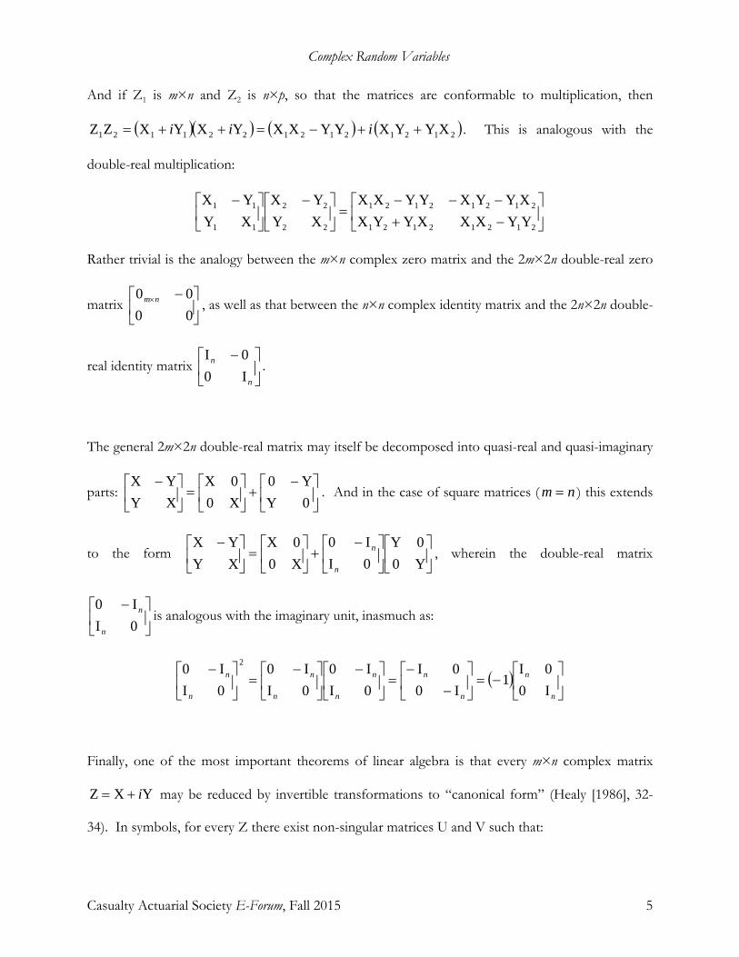
And if Z1 is m×n and Z2 is n×p, so that the matrices are conformable to multiplication, then
( )( ) ( ) ( )21212121221121 XYYXYYXXYXYXZZ ++−=++= iii . This is analogous with the
double-real multiplication:
−+−−−
=
−
−
21212121
21212121
22
22
11
11
YYXXXYYXXYYXYYXX
XYYX
XYYX
Rather trivial is the analogy between the m×n complex zero matrix and the 2m×2n double-real zero
matrix
−×
0000 nm , as well as that between the n×n complex identity matrix and the 2n×2n double-
real identity matrix
−
n
n
I00I
.
The general 2m×2n double-real matrix may itself be decomposed into quasi-real and quasi-imaginary
parts:
−+
=
−0YY0
X00X
XYYX
. And in the case of square matrices ( nm = ) this extends
to the form
−+
=
−Y00Y
0II0
X00X
XYYX
n
n , wherein the double-real matrix
−0II0
n
n is analogous with the imaginary unit, inasmuch as:
( )
−=
−
−=
−
−=
−
n
n
n
n
n
n
n
n
n
n
I00I
1I00I
0II0
0II0
0II0 2
Finally, one of the most important theorems of linear algebra is that every m×n complex matrix
YXZ i+= may be reduced by invertible transformations to “canonical form” (Healy [1986], 32-
34). In symbols, for every Z there exist non-singular matrices U and V such that:

Complex Random Variables
Casualty Actuarial Society E-Forum, Fall 2015 6
nm
rnnnmmm
××××
=
000I
VZU
The m×n real matrix on the right side of the equation consists entirely of zeroes except for r
instances of one along its main diagonal. Since invertible matrix operations can reposition the ones,
it is further stipulated that the ones appear as a block in the upper-left corner. Although many
reductions of Z to canonical form exist, the canonical forms themselves must all contain the same
number of ones, r, which is defined as the rank of Z. Providing the matrices with real and complex
parts, we have:
( )( )( )( ) ( )
nmr
nnnmmm
i
ii
iii
×
×××
+
=
+=++−+−−−=
+++=
0000IBA
QXRPYRQYSPXSQXSPYSQYRPXRSRYXQPVZU
The double-real analogue to this is:
=
−=
−
−
−
×
×
000I
0
0000I
ABBA
RSSR
XYYX
PQQP
rnm
nmr
As shown in the previous section,
−PQQP
is non-singular, or invertible, if and only if
QPU i+= is non-singular; the same is true for
−RSSR
. Therefore, the rank of the double-real
analogue of a complex matrix is twice the rank of the complex matrix. Moreover, the 2r instances of
one correspond to r quasi-real and r quasi-imaginary instances. It is not possible for the
contribution to the rank of a matrix to be real without its being imaginary, and vice versa.
Complex Random Variables
Casualty Actuarial Society E-Forum, Fall 2015 7
To conclude this section, there are extensive analogies between complex and double-real matrices,
analogies so extensive that one who lacked either the confidence or the software to work with
complex numbers could probably do a work-around with double-real matrices.2
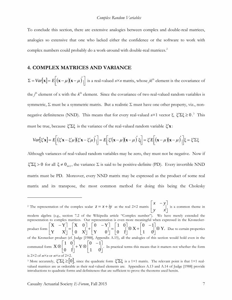
4. COMPLEX MATRICES AND VARIANCE
[ ] ( )( )
′−−==Σ µµ xxx EVar is a real-valued n×n matrix, whose jkth element is the covariance of
the jth element of x with the kth element. Since the covariance of two real-valued random variables is
symmetric, Σ must be a symmetric matrix. But a realistic Σ must have one other property, viz., non-
negative definiteness (NND). This means that for every real-valued n×1 vector ξ, 0Σξξ ≥′ .3 This
must be true, because Σξξ′ is the variance of the real-valued random variable xξ′ :
[ ] ( )( ) ( )( ) ( )( ) ξξξξξξξξξξξ Σ′=
′−−′=
′−−′=
′′−′′−′=′ µµµµµµ xxxxxxx EEEVar
Although variances of real-valued random variables may be zero, they must not be negative. Now if
0Σξξ >′ for all 10ξ ×≠ n , the variance Σ is said to be positive-definite (PD). Every invertible NND
matrix must be PD. Moreover, every NND matrix may be expressed as the product of some real
matrix and its transpose, the most common method for doing this being the Cholesky
2 The representation of the complex scalar iyxz += as the real 2×2 matrix
−xyyx
is a common theme in
modern algebra (e.g., section 7.2 of the Wikipedia article “Complex number”). We have merely extended the representation to complex matrices. Our representation is even more meaningful when expressed in the Kronecker-
product form Y.0110
X1001
0YY0
X00X
XYYX
⊗
−+⊗
=
−+
=
− Due to certain properties
of the Kronecker product (cf. Judge [1988], Appendix A.15), all the analogies of this section would hold even in the
commuted form
−⊗+
⊗
0110
Y1001
X . In practical terms this means that it matters not whether the form
is 2×2 of m×n or m×n of 2×2. 3 More accurately, [ ]0Σξξ ≥′ , since the quadratic form Σξξ′ is a 1×1 matrix. The relevant point is that 1×1 real-valued matrices are as orderable as their real-valued elements are. Appendices A.13 and A.14 of Judge [1988] provide introductions to quadratic forms and definiteness that are sufficient to prove the theorems used herein.
Complex Random Variables
Casualty Actuarial Society E-Forum, Fall 2015 8
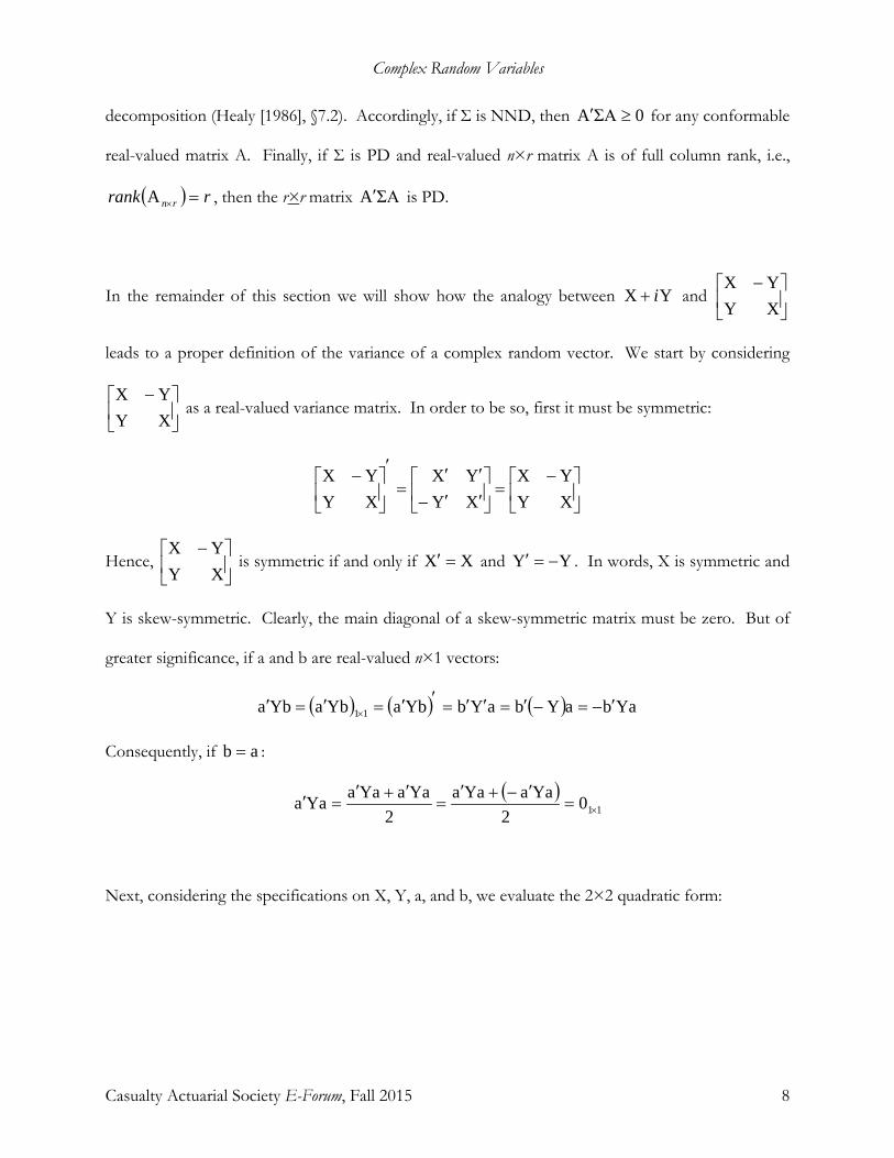
decomposition (Healy [1986], §7.2). Accordingly, if Σ is NND, then 0ΣAA ≥′ for any conformable
real-valued matrix A. Finally, if Σ is PD and real-valued n×r matrix A is of full column rank, i.e.,
( ) rrank rn =×A , then the r×r matrix ΣAA′ is PD.
In the remainder of this section we will show how the analogy between YX i+ and
−XYYX
leads to a proper definition of the variance of a complex random vector. We start by considering
−XYYX
as a real-valued variance matrix. In order to be so, first it must be symmetric:
−=
′′−
′′=
′
−XYYX
XYYX
XYYX
Hence,
−XYYX
is symmetric if and only if XX =′ and YY −=′ . In words, X is symmetric and
Y is skew-symmetric. Clearly, the main diagonal of a skew-symmetric matrix must be zero. But of
greater significance, if a and b are real-valued n×1 vectors:
( ) ( ) ( ) YabaYbaYbYbaYbaYba 11 ′−=−′=′′=′′=′=′ ×
Consequently, if ab = :
( )110
2YaaYaa
2YaaYaaYaa ×=
′−+′=
′+′=′
Next, considering the specifications on X, Y, a, and b, we evaluate the 2×2 quadratic form:
Complex Random Variables
Casualty Actuarial Society E-Forum, Fall 2015 9
−′
−′
=
′+′−′+′
′+′−′+′=
′+′−′+′′+′−
′+′−′+′−′+′=
′+′−′+′+′++′−−′+−′−′+′−′+′
=
′+′−′+′′+′+′+′−
′−′+′−′−′+′−′+′=
−
′+′′+′−
′−′′+′=
−
−
′′−
′′=
−
−′
−
ba
XYYX
ba
0
0ba
XYYX
ba
XbbYbaYabXaa00XbbYbaYabXaa
XbbYbaYabXaaXbaXabXabXbaXbbYbaYabXaa
XbbYbaYabXaa0Xba0Xab0Xab0XbaXbbYbaYabXaa
XbbYbaYabXaaYbbXbaYaaXabYaaXabYbbXbaXbbYbaYabXaa
abba
YbXaYaXbYaXbYbXa
abba
XYYX
abba
abba
XYYX
abba
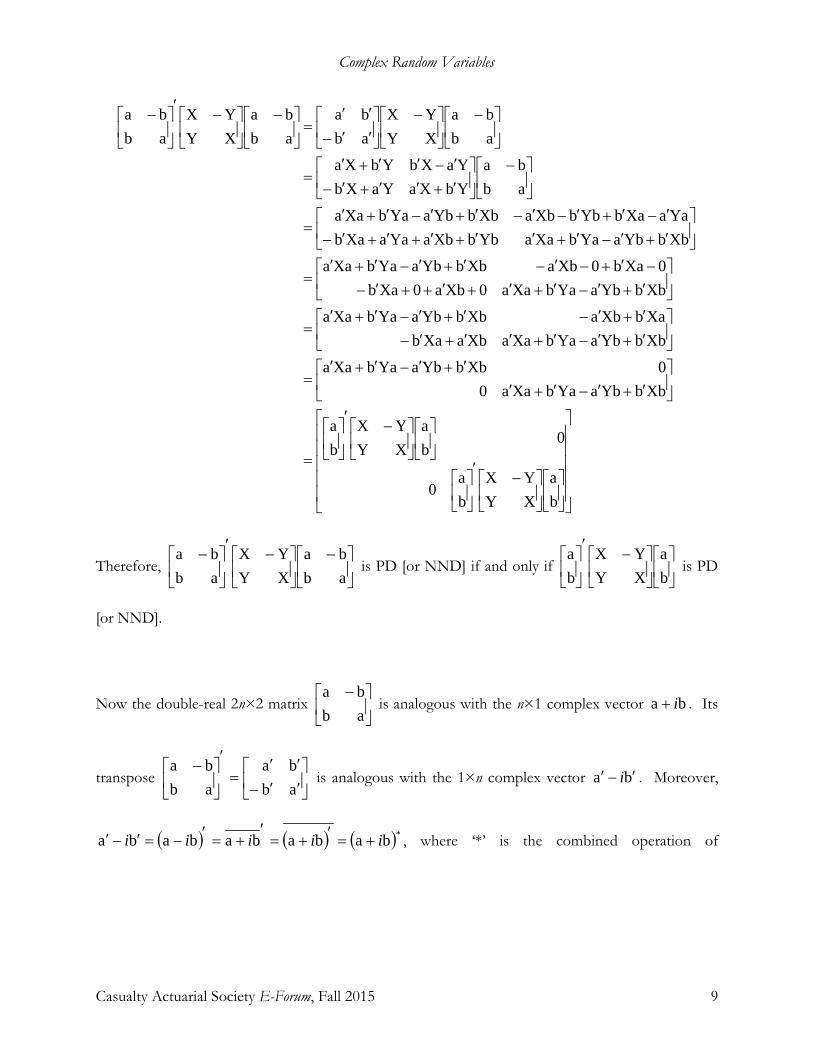
Therefore,
−
−′
−abba
XYYX
abba
is PD [or NND] if and only if
−′
ba
XYYX
ba
is PD
[or NND].
Now the double-real 2n×2 matrix
−abba
is analogous with the n×1 complex vector ba i+ . Its
transpose
′′−
′′=
′
−abba
abba
is analogous with the 1×n complex vector ba ′−′ i . Moreover,
( ) ( ) ( )*bababababa iiiii +=′+=′
+=′−=′−′ , where ‘*’ is the combined operation of
Complex Random Variables
Casualty Actuarial Society E-Forum, Fall 2015 10
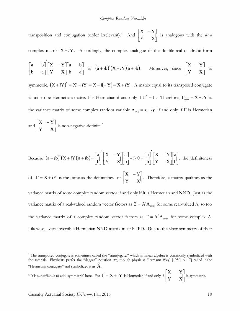
transposition and conjugation (order irrelevant).4 And
−XYYX
is analogous with the n×n
complex matrix YX i+ . Accordingly, the complex analogue of the double-real quadratic form
−
−′
−abba
XYYX
abba
is ( ) ( )( )baYXba * iii +++ . Moreover, since
−XYYX
is
symmetric, ( ) ( ) YXYXYXYX * iiii +=−−=′−′=+ . A matrix equal to its transposed conjugate
is said to be Hermetian: matrix Γ is Hermetian if and only if Γ=Γ* . Therefore, YX inn +=Γ × is
the variance matrix of some complex random variable yxz in +=×1 if and only if Γ is Hermetian
and
−XYYX
is non-negative-definite.5
Because ( ) ( )( )
−′
=⋅+
−′
=+++
ba
XYYX
ba
0ba
XYYX
ba
baYXba * iiii , the definiteness
of YX i+=Γ is the same as the definiteness of
−XYYX
. Therefore, a matrix qualifies as the
variance matrix of some complex random vector if and only if it is Hermetian and NND. Just as the
variance matrix of a real-valued random vector factors as nn×′=Σ AA for some real-valued A, so too
the variance matrix of a complex random vector factors as nn×=Γ AA* for some complex A.
Likewise, every invertible Hermetian NND matrix must be PD. Due to the skew symmetry of their
4 The transposed conjugate is sometimes called the “transjugate,” which in linear algebra is commonly symbolized with the asterisk. Physicists prefer the “dagger” notation A†, though physicist Hermann Weyl [1950, p. 17] called it the
“Hermetian conjugate” and symbolized it as A~ .
5 It is superfluous to add ‘symmetric’ here. For YX i+=Γ is Hermetian if and only if
−XYYX
is symmetric.

Complex Random Variables
Casualty Actuarial Society E-Forum, Fall 2015 11
complex parts, the main diagonals of Hermetian matrices must be real-valued. If the matrices are
NND [or PD], all the elements of their main diagonals must be non-negative [or positive].
Let Γ represent the variance of the complex random vector z. Its jkth element represents the
covariance of the jth element of z with the kth element. Since Γ is Hermetian,
[ ] [ ] [ ] [ ] [ ] jkjkjkkjkjkjkj γγ =Γ=Γ=Γ′=Γ=Γ= * . Because of this, it is fitting and natural to define
the variance of a complex random vector as:
[ ] ( )( ) ( )( )[ ]*µµµµ −−=
′
−−==Γ zzzzz EEVar
The complex formula is like the real formula except that the second factor in the expectation is
transjugated, not simply transposed. This renders Γ Hermetian, since:
( )( )[ ] ( )( ){ }[ ] ( )( )[ ] Γ=−−=−−=−−=Γ ****** µµµµµµ zzzzzz EEE
It also renders Γ NND. For since ( )( )*zz µµ −− is NND, its expectation over the probability
distribution of z must also be so. Usually Γ is PD, in which case 1−Γ exists.
5. THE EXPECTATION OF THE STANDARD QUADRATIC FORM
The most common quadratic form in zn×1 involves the variance of the complex random variable,
viz., ( ) ( )µµ −Γ− − zz 1* , where [ ]zVar=Γ . The expectation of this quadratic form equals n, the
rank of the variance. The following proof uses the trace function. The trace of a matrix is the sum
of its main-diagonal elements, and if A and B are conformable ( ) ( )BAtrABtr = . Moreover, the
trace of the expectation equals the expectation of the trace. Consequently:
Complex Random Variables
Casualty Actuarial Society E-Forum, Fall 2015 12
( ) ( )[ ] ( ) ( )( )[ ]( )( )( )[ ]( )( )[ ]( )( )( )[ ]( )
( )( )
ntrtr
Etr
Etr
trE
trEE
n
==
ΓΓ=
−−Γ=
−−Γ=
−−Γ=
−Γ−=−Γ−
−
−
−
−
−−
I
1
*1
*1
*1
1*1*
µµ
µµ
µµ
µµµµ
zz
zz
zz
zzzz
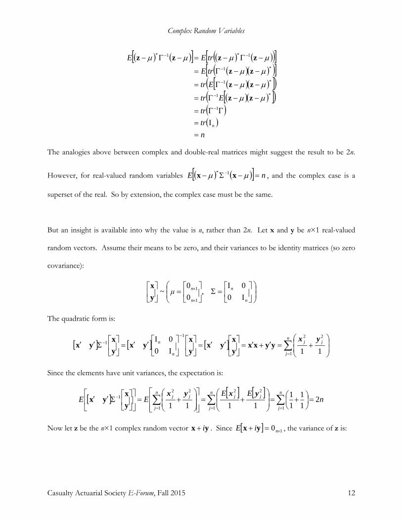
The analogies above between complex and double-real matrices might suggest the result to be 2n.
However, for real-valued random variables ( ) ( )[ ] nE =−Σ− − µµ xx 1* , and the complex case is a
superset of the real. So by extension, the complex case must be the same.
But an insight is available into why the value is n, rather than 2n. Let x and y be n×1 real-valued
random vectors. Assume their means to be zero, and their variances to be identity matrices (so zero
covariance):
=Σ
=
×
×
n
n
n
nμI00I
,00
~1
1
yx
The quadratic form is:
[ ] [ ] [ ] ∑=
−
−
+=′+′=
′′=
′′=
Σ′′
n
j
jj
n
n
1
2211
11I00I yx
yyxxyx
yxyx
yxyx
yx
Since the elements have unit variances, the expectation is:
[ ] [ ] [ ]n
EEEE
n
j
n
j
jjn
j
jj 211
11
1111 11
22
1
221 =
+=
+=
+=
Σ′′ ∑∑∑
===
− yxyxyx
yx
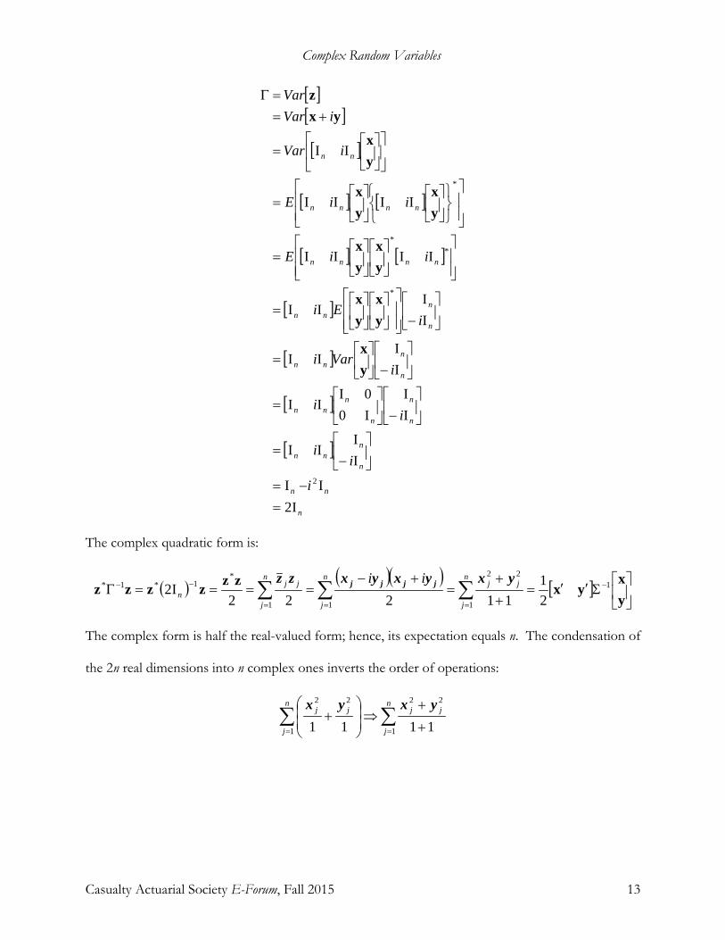
Now let z be the n×1 complex random vector yx i+ . Since [ ] 10 ×=+ niE yx , the variance of z is:
Complex Random Variables
Casualty Actuarial Society E-Forum, Fall 2015 13
[ ][ ]
[ ]
[ ] [ ]
[ ] [ ]
[ ]
[ ]
[ ]
[ ]
n
nn
n
nnn
n
n
n
nnn
n
nnn
n
nnn
nnnn
nnnn
nn
i
ii
ii
iVari
iEi
iiE
iiE
iVar
iVarVar
I2II
II
II
II
I00I
II
II
II
II
II
IIII
IIII
II
2
*
**
*
=−=
−
=
−
=
−
=
−
=
=
=
=
+==Γ
yx
yx
yx
yx
yx
yx
yx
yx
yxz
The complex quadratic form is:
( ) ( )( ) [ ]
Σ′′=
+
+=
+−====Γ −
===
−− ∑∑∑ yx
yxzzzzzz 1
1
22
11
*1*1*
21
11222I2
n
j
jjn
j
n
j
jjn
ii yxyxyxzz jjjj
The complex form is half the real-valued form; hence, its expectation equals n. The condensation of
the 2n real dimensions into n complex ones inverts the order of operations:
∑∑== +
+⇒
+
n
j
jjn
j
jj
1
22
1
22
1111yxyx
Complex Random Variables
Casualty Actuarial Society E-Forum, Fall 2015 14
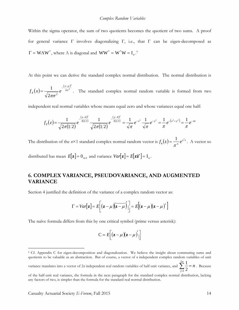
Within the sigma operator, the sum of two quotients becomes the quotient of two sums. A proof
for general variance Γ involves diagonalizing Γ, i.e., that Γ can be eigen-decomposed as
*WWΛ=Γ , where Λ is diagonal and nIWWWW ** == .6
At this point we can derive the standard complex normal distribution. The normal distribution is
( )( )
2
2
222
1 σµ
πσ
−−
=x
X exf . The standard complex normal random variable is formed from two
independent real normal variables whose means equal zero and whose variances equal one half:
( )( )
( )( )
( )
( )( ) ( ) zzyxyx
yx
Z eeeeeezf −+−−−−
−−
−
====ππππππ1111
2121
2121 2222
22
2120
2120
The distribution of the n×1 standard complex normal random vector is ( ) zz*1z ef nπ=z . A vector so
distributed has mean [ ] 10 ×= nE z and variance [ ] [ ] nEVar I=′= zzz .
6. COMPLEX VARIANCE, PSEUDOVARIANCE, AND AUGMENTED VARIANCE
Section 4 justified the definition of the variance of a complex random vector as:
[ ] ( )( ) ( )( )[ ]*µµµµ −−=
′
−−==Γ zzzzz EEVar
The naïve formula differs from this by one critical symbol (prime versus asterisk):
( )( )
′−−= µµ zzEC
6 Cf. Appendix C for eigen-decomposition and diagonalization. We believe the insight about commuting sums and quotients to be valuable as an abstraction. But of course, a vector of n independent complex random variables of unit
variance translates into a vector of 2n independent real random variables of half-unit variance, and nn
j=∑
=
2
1 21
. Because
of the half-unit real variance, the formula in the next paragraph for the standard complex normal distribution, lacking any factors of two, is simpler than the formula for the standard real normal distribution.
Complex Random Variables
Casualty Actuarial Society E-Forum, Fall 2015 15
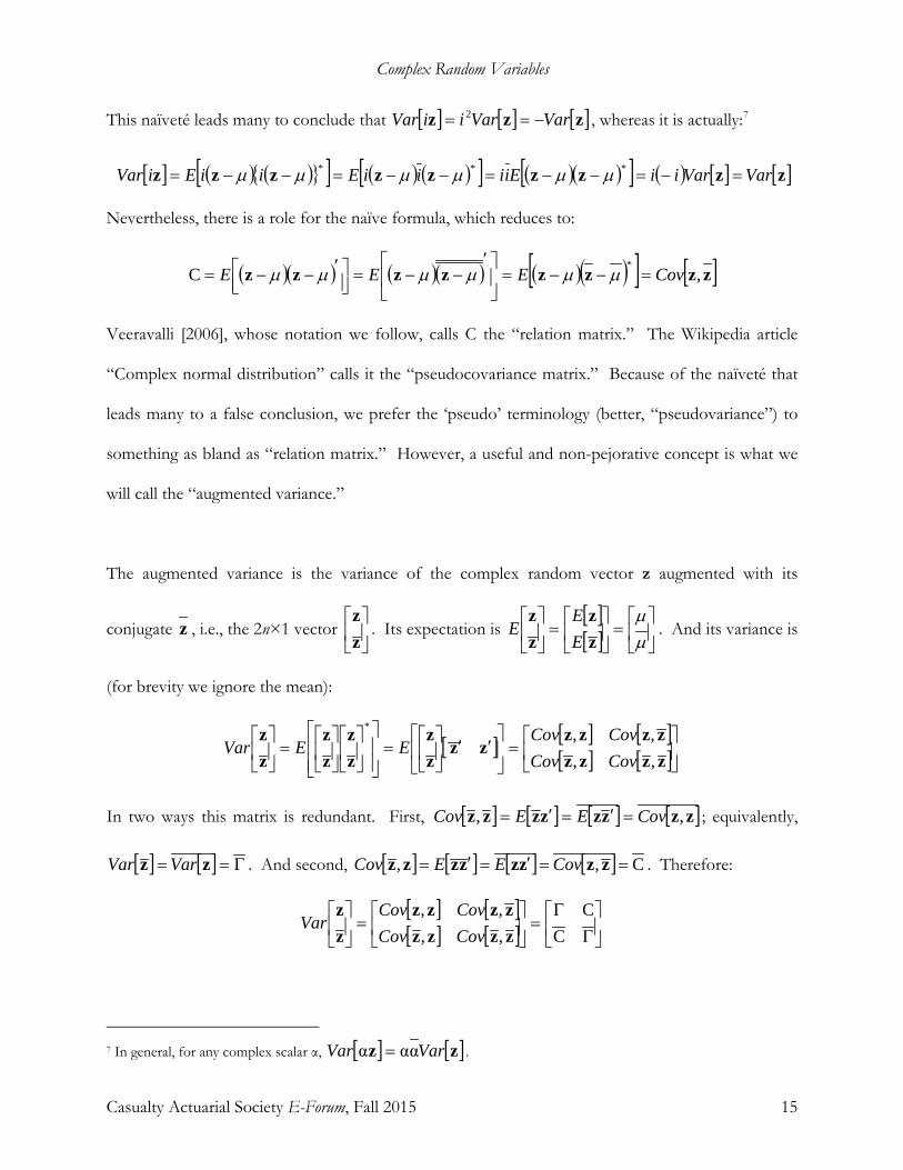
This naïveté leads many to conclude that [ ] [ ] [ ]zzz VarVariiVar −== 2 , whereas it is actually:7
[ ] ( ) ( ){ }[ ] ( ) ( )[ ] ( )( )[ ] ( ) [ ] [ ]zzzzzzzzz VarVariiEiiiiEiiEiVar =−=−−=−−=−−= *** µµµµµµ
Nevertheless, there is a role for the naïve formula, which reduces to:
( )( ) ( )( ) ( )( )[ ] [ ]zzzzzzzz ,C*
CovEEE =−−=
′−−=
′−−= µµµµµµ
Veeravalli [2006], whose notation we follow, calls C the “relation matrix.” The Wikipedia article
“Complex normal distribution” calls it the “pseudocovariance matrix.” Because of the naïveté that
leads many to a false conclusion, we prefer the ‘pseudo’ terminology (better, “pseudovariance”) to
something as bland as “relation matrix.” However, a useful and non-pejorative concept is what we
will call the “augmented variance.”
The augmented variance is the variance of the complex random vector z augmented with its
conjugate z , i.e., the 2n×1 vector
zz
. Its expectation is [ ][ ]
=
=
µµ
zz
zz
EE
E . And its variance is
(for brevity we ignore the mean):
[ ] [ ] [ ][ ] [ ]
=
′′
=
=
zzzzzzzz
zzzz
zz
zz
zz
,,,,*
CovCovCovCov
EEVar
In two ways this matrix is redundant. First, [ ] [ ] [ ] [ ]zzzzzzzz ,, CovEECov =′=′= ; equivalently,
[ ] [ ] Γ== zz VarVar . And second, [ ] [ ] [ ] [ ] C,, ==′=′= zzzzzzzz CovEECov . Therefore:
[ ] [ ][ ] [ ]
Γ
Γ=
=
C
C,,,,zzzzzzzz
zz
CovCovCovCov
Var
7 In general, for any complex scalar α, [ ] [ ]zz VarVar ααα = .

Complex Random Variables
Casualty Actuarial Society E-Forum, Fall 2015 16
As with any valid variance matrix, the augmented variance must be Hermetian. Hence,
Γ′′Γ
=′
ΓΓ
=′
Γ
Γ=
Γ
Γ=
Γ
Γ*
**
CC
CC
CC
CC
CC
, from which follow Γ=Γ* and CC =′ .
Moreover, it must be at least NND, if not PD. It is important to note from this that the
pseudovariance is an essential part of the augmented z; it is possible for two random variables to
have the same variance and to covary differently with their conjugates. How a complex random
vector covaries with its conjugate is useful information; it is even a parameter of the general complex
normal distribution, which we will treat next.
7. THE COMPLEX NORMAL DISTRIBUTION
All the information for deriving the complex normal distribution of yxz in +=×1 is contained in
the parameters of the real-valued multivariate normal distribution:
ΣΣΣΣ
=Σ
=
××
yyyx
xyxx
y
x
yx
nnnN 2212 ,μμ
μ~
According to this variance structure, the real and imaginary parts of z may covary, as long as the
covariance is symmetric: xyyx Σ′=Σ . The grand Σ matrix must be symmetric and PD. The
probability density function of this multivariate normal is:8
( )( )
[ ] [ ]
−−
Σ′−′′−′−
−−
Σ′−′′−′−
−−
Σ=
Σ= y
xyx
y
xyx
yx
μyμx
μyμx21
2
μyμx
μyμx21
2
11
21
2
1y,x eefnnn ππ
8 As derived briefly by Judge [1988, pp 49f]. Chapter 4 of Johnson [1992] is thorough. To be precise, Σ under the
radical should be Σ , the absolute value of the determinant of Σ. However, the determinant of a PD matrix must be positive (cf. Judge [1988, A.14(1)]).

Complex Random Variables
Casualty Actuarial Society E-Forum, Fall 2015 17
Since yxz i+= , the augmented vector is
Ξ=
−
=
−+
=
yx
yx
yxyx
zz
nnn
nn
ii
ii
IIII
. We will call
−
=Ξnn
nnn i
iIIII
the augmentation matrix; this linear function of the real-valued vectors produces
the complex vector and its conjugate. An important equation is:
nn
n
nn
nn
nn
nnnn iii
i2
* I22I002I
IIII
IIII
=
=
−
−
=ΞΞ
Therefore, Ξn has an inverse, viz., one half of its transjugate.
The augmented mean is
=
−+
=
Ξ=
μμ
μμμμ
μμ
yx
yx
y
x
zz
ii
E n . The augmented variance is:
( ) ( )( ) ( )
Γ
Γ=
Σ−Σ+Σ+ΣΣ+Σ−Σ−ΣΣ+Σ+Σ−ΣΣ−Σ−Σ+Σ
=
−
Σ−ΣΣ−ΣΣ+ΣΣ+Σ
=
−
ΣΣΣΣ
−
=
ΣΞΞ=
CC
IIII
IIII
IIII
xyxx
*
yxxyyyxxyxxyyyxx
yxxyyyxxyxxyyyxx
yyyx
yyxyyxxx
yyyx
xyxx
zz
iiii
iiiiii
iiii
Var
nn
nn
nn
nn
nn
nn
nn
And so:
( ) ( ) ( ) 111*1*1
1
CC −−−−
−− ΞΣΞ=ΣΞΞ=
Γ
Γ=
nnnnVar
zz
This can be reformulated as 11
*1*
CC −
−− Σ=Ξ
Γ
ΓΞ=Ξ
Ξ nnnnVar
zz
.
Complex Random Variables
Casualty Actuarial Society E-Forum, Fall 2015 18
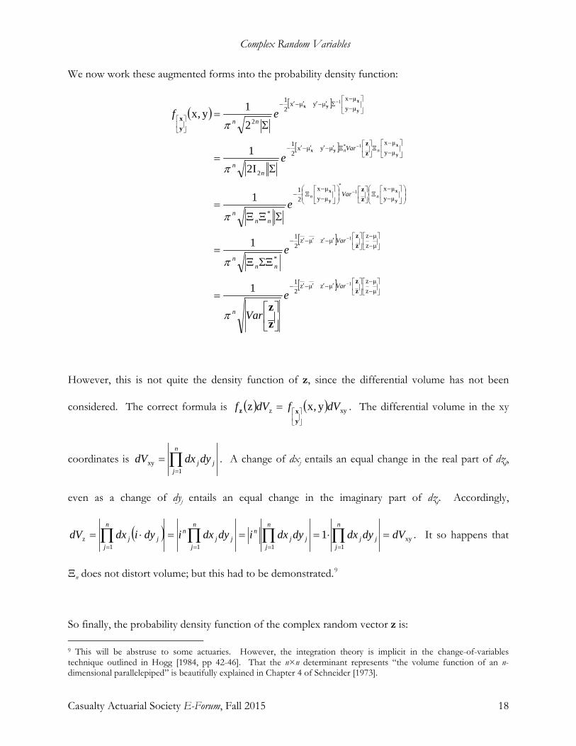
We now work these augmented forms into the probability density function:
( )[ ]
[ ]
[ ]
[ ]
−−
′−′′−′−
−−
′−′′−′−
−−
Ξ
−−
Ξ−
−−
Ξ
Ξ′−′′−′−
−−
Σ′−′′−′−
−
−
−
−
−
=
ΣΞΞ=
ΣΞΞ=
Σ=
Σ=
μzμz
μzμz21
μzμz
μzμz21
*
μyμx
μyμx
21
*
μyμx
μyμx21
2
μyμx
μyμx21
2
1
1
1*
1*
1
1
1
1
I21
21y,x
zz
zz
zz
zz
yx
zz
y
x
y
x
y
xyx
y
xyx
Var
n
Var
nnn
Var
nnn
Var
nn
nn
e
Var
e
e
e
ef
nn
nn
π
π
π
π
π
However, this is not quite the density function of z, since the differential volume has not been
considered. The correct formula is ( ) ( ) xyz y,xz dVfdVf
=yxz . The differential volume in the xy
coordinates is ∏=
=n
jjj dydxdV
1xy . A change of dxj entails an equal change in the real part of dzj,
even as a change of dyj entails an equal change in the imaginary part of dzj. Accordingly,
( ) xy1111
z 1 dVdydxdydxidydxidyidxdVn
jjj
n
jjj
nn
jjj
nn
jjj =⋅===⋅= ∏∏∏∏
====
. It so happens that
Ξn does not distort volume; but this had to be demonstrated.9
So finally, the probability density function of the complex random vector z is: 9 This will be abstruse to some actuaries. However, the integration theory is implicit in the change-of-variables technique outlined in Hogg [1984, pp 42-46]. That the n×n determinant represents “the volume function of an n-dimensional parallelepiped” is beautifully explained in Chapter 4 of Schneider [1973].

Complex Random Variables
Casualty Actuarial Society E-Forum, Fall 2015 19
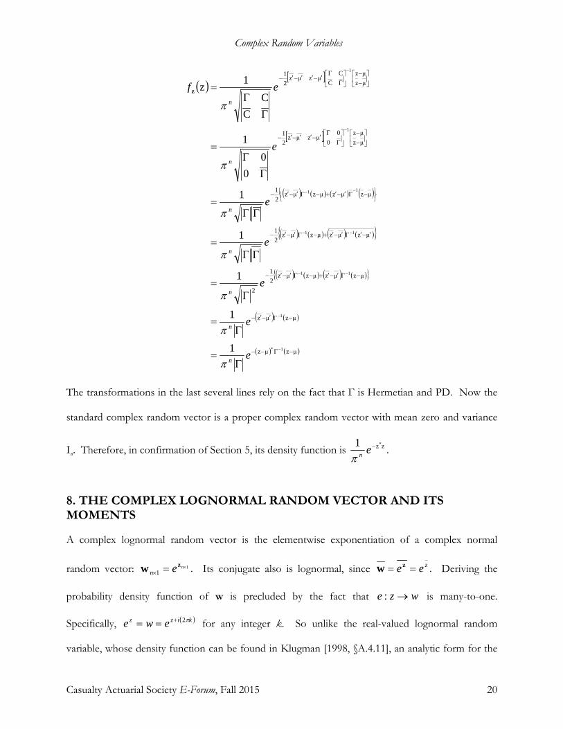
( ) ( ) ( ) ( )
[ ]
[ ]
−−
Γ
Γ′−′′−′−
−−
′−′′−′−
−
−
ΓΓ
=
=
==⋅=
μzμz
CC
μzμz21
μzμz
μzμz21
xy
z
1
1
CC
1
1
y,xz1zz
e
e
Var
fdVdVfff
n
Var
n
π
π
zz
yxzzz
zz
This formula is equivalent to the one found in the Wikipedia article “Complex normal distribution.”
Although CC 1−Γ−ΓΓ appears within the radical of that article’s formula, it can be shown that
CCC
C 1−Γ−ΓΓ=Γ
Γ. As far as allowable parameters are concerned, µ may be any complex
vector. Γ
ΓC
C is allowed if and only if Σ=Ξ
Γ
ΓΞ 4
CC*
nn is real-valued and PD.
Veeravalli [2006] defines a “proper” complex variable as one whose pseudo[co]variance matrix is
0n×n. Inserting zero for C into the formula, we derive the probability density function of a proper
complex random variable whose variance is Γ:
Complex Random Variables
Casualty Actuarial Society E-Forum, Fall 2015 20
( )[ ]
[ ]
( ) ( ) ( ) ( )
( ) ( ) ( ) ( ){ }
( ) ( ) ( ) ( ){ }
( ) ( )
( ) ( )μzμz
μzμz
μzμzμzμz21
2
μzμzμzμz21
μzμzμzμz21
μzμz
00
μzμz21
μzμz
CC
μzμz21
1*
1
11
11
11
1
1
1
1
1
1
1
00
1
CC
1z
−Γ−−
−Γ′−′−
−Γ′−′+−Γ′−′−
′−′Γ′−′+−Γ′−′−
−Γ′−′+−Γ′−′−
−−
Γ
Γ′−′′−′−
−−
Γ
Γ′−′′−′−
−
−
−−
−−
−−
−
−
Γ=
Γ=
Γ=
ΓΓ=
ΓΓ=
ΓΓ
=
ΓΓ
=
e
e
e
e
e
e
ef
n
n
n
n
n
n
n
π
π
π
π
π
π
πz
The transformations in the last several lines rely on the fact that Γ is Hermetian and PD. Now the
standard complex random vector is a proper complex random vector with mean zero and variance
In. Therefore, in confirmation of Section 5, its density function is zz*1 −enπ.
8. THE COMPLEX LOGNORMAL RANDOM VECTOR AND ITS MOMENTS
A complex lognormal random vector is the elementwise exponentiation of a complex normal
random vector: 11
×=×nen
zw . Its conjugate also is lognormal, since zee == zw . Deriving the
probability density function of w is precluded by the fact that wze →: is many-to-one.
Specifically, ( )kizz ewe π2+== for any integer k. So unlike the real-valued lognormal random
variable, whose density function can be found in Klugman [1998, §A.4.11], an analytic form for the

Complex Random Variables
Casualty Actuarial Society E-Forum, Fall 2015 21
complex lognormal density is not available. However, even for the real-valued lognormal the
density function is of little value; its moments are commonly derived from the moment generating
function of the normal variable on which it is based. So too, the moment generating function of the
complex normal random vector is available for deriving the lognormal moments.
We hereby define the moment generating function of the complex n×1 random vector z as
( ) [ ]zzz
ts11 t,s ′+′×× = eEM nn . Since this definition may differ from other definitions in the sparse
literature, we should justify it. First, because we will take derivatives of this function with respect to
s and t, the function must be differentiable. This demands simple transposition in the linear
combination, i.e., zz ts ′+′ rather than the transjugation zz ** ts + . For transjugation would involve
derivatives of the form dssd , which do not exist, as they violate the Cauchy-Riemann condition.10
Second, even though moments of z are conjugates of moments of z, we will need second-order
moments involving both z and z . For this reason both terms must be in the exponent of the
moment generating function.
10 Cf. Appendix D.1.3 of Havil [2003]. Express ( )iyxzf += in terms of real-valued functions, i.e., as
( ) ( )yxviyxu ,, ⋅+ . The derivative is based on the matrix of real-valued partial derivatives
∂∂∂∂∂∂∂∂yvyuxvxu
.
For the derivative to be the same in both directions, the Cauchy-Riemann condition must hold, viz., that
yvxu ∂∂=∂∂ and yuxv ∂∂−=∂∂ . But for ( ) iyxzzf −== , the partial-derivative matrix is
−10
01;
hence yvxu ∂∂≠∂∂ . The Cauchy-Riemann condition becomes intuitive when one regards a valid complex
derivative as a double-real 2×2 matrix (Section 3). Compare this with ( ) iyxzzf +== , whose matrix is
1001
,
which represents the complex number 1.
Complex Random Variables
Casualty Actuarial Society E-Forum, Fall 2015 22
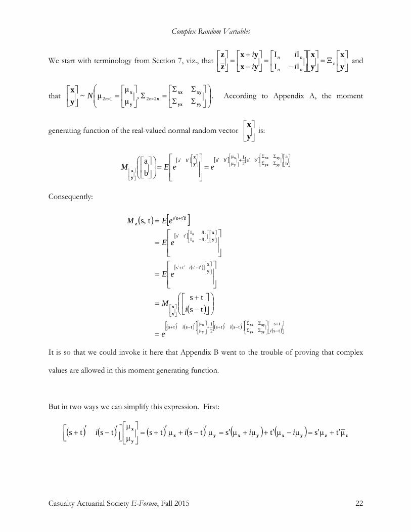
We start with terminology from Section 7, viz., that
Ξ=
−
=
−+
=
yx
yx
yxyx
zz
nnn
nn
ii
ii
IIII
and
that
ΣΣΣΣ
=Σ
=
××
yyyx
xyxx
y
x
yx
nnnN 2212 ,μμ
μ~ . According to Appendix A, the moment
generating function of the real-valued normal random vector
yx
is:
[ ] [ ] [ ]
ΣΣΣΣ
′′+
′′
′′
=
=
ba
ba21
μμ
baba
ba
yyyx
xyxx
y
x
yx
yx eeEM
Consequently:
( ) [ ][ ]
( )[ ]
( )
( ) ( )[ ] ( ) ( )[ ] ( )
−+
ΣΣΣΣ′−′++
′−′+
′−′′+′
−
′′
′+′
=
−+
=
=
=
=
tsts
tsts21
μμ
tsts
tsts
IIII
ts
ts
tsts
ts,
iii
i
ii
e
iM
eE
eE
eEM
nn
nn
yyyx
xyxx
y
x
yx
yx
yx
zzz
It is so that we could invoke it here that Appendix B went to the trouble of proving that complex
values are allowed in this moment generating function.
But in two ways we can simplify this expression. First:
( ) ( ) ( ) ( ) ( ) ( ) zzyxyxyxy
x μtμsμμtμμsμtsμtsμμ
tsts ′+′=−′++′=′−+′+=
′−′+ iiii
Complex Random Variables
Casualty Actuarial Society E-Forum, Fall 2015 23
And second, again from Section 7, **22C
CnnnnnnVar Ξ
ΣΣΣΣ
Ξ=ΞΣΞ=
Γ
Γ=
×
yyyx
xyxx
zz
, or
equivalently,
ΣΣΣΣ
=Ξ
Γ
ΓΞ
yyyx
xyxx
2CC
2
*nn . Hence:
( ) ( ) ( ) ( ) ( ) ( )
−+Ξ
Γ
ΓΞ
′−′+=
−+
ΣΣΣΣ
′−′+
tsts
2CC
2tsts
tsts
tsts*
ii
ii nn
yyyx
xyxx
On the right side, ( ) ( )( ) ( )( ) ( )
=
−++−−+
=
−+
−
=
−+Ξ
st
tstststs
21
tsts
IIII
21
tsts
2 iii
i nn
nnn . And on the
left side, ( ) ( ) ( ) ( ) [ ]tsIIII
tsts21
2tsts
*
′′=
−
′−′+=
Ξ
′−′+
nn
nnn
iiii . So:
( ) ( ) ( ) [ ]
Γ
Γ′′=
−+
ΣΣΣΣ
′−′+
st
CC
tststs
tstsi
iyyyx
xyxx
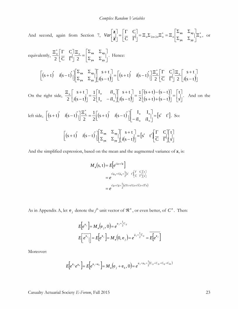
And the simplified expression, based on the mean and the augmented variance of z, is:
( ) [ ][ ]
( )sttCtCssts21μtμs
st
CC
ts21μtμs
tsts,
Γ′+′+′+Γ′+′+′
Γ
Γ′′+′+′
′+′
=
=
=
e
e
eEM
zz
zzz
As in Appendix A, let je denote the jth unit vector of nℜ , or even better, of nC . Then:
[ ] ( )
[ ] ( ) [ ]jjjjjj
jjjj
eEeMeEeE
eMeE
j
j
zz
zz
zz
====
==
+
+
C21μ
C21μ
e0,
0,e
Moreover:
[ ] [ ] ( ) ( )kkkjjkjjkjkjkj eMeEeeE kj
CCCC21μμ
0,ee++++++ =+== z
zzzz
Complex Random Variables
Casualty Actuarial Society E-Forum, Fall 2015 24
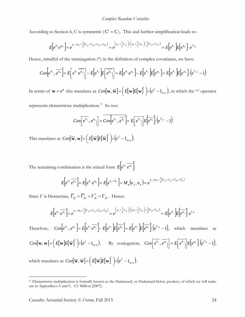
According to Section 6, C is symmetric ( CC =′ ). This and further simplification leads to:
[ ] ( ) ( ) [ ] [ ] jkkjjkjkkkkjjjkkkjjkjjkj
kj eeEeEeeeeE CCC21C
21μC
21μCCCC
21μμ
⋅===++
++
++++++ zzzz
Hence, mindful of the transjugation (*) in the definition of complex covariance, we have:
[ ] [ ] [ ] [ ] [ ] [ ] [ ] ( )1, C −⋅=−=
−
= jkkjkjkjkjkjkj eeEeEeEeEeeEeEeEeeEeeCov zzzzzzzzzzzz
In terms of zw e= this translates as [ ] [ ] [ ] ( )nneEECov ×−
′= 1, Cwwww , in which the ‘◦’ operator
represents elementwise multiplication.11 So too:
[ ] [ ] ( )1,, C −⋅
==
jkkjkjkj eeEeEeeCoveeCov zzzzzz
This translates as [ ] [ ] [ ] ( )nneEECov ×−
′= 1, Cwwww .
The remaining combination is the mixed form [ ]kj eeE zz :
[ ] [ ] [ ] ( ) ( )kjkkjjjkkjkjkjkj eMeEeeEeeE kj
Γ+++Γ+++ ====CC
21μμ
e,ezzzzzzz
Since Γ is Hermetian, jkjkjkkj Γ=Γ=Γ′=Γ * . Hence:
[ ] ( ) ( ) [ ] [ ] jkkjjkjkkkkjjjkjkkjjjkkj
kj eeEeEeeeeE ΓΓ+Γ+
++
+Γ+++Γ++
⋅=== zzzz 21C
21μC
21μCC
21μμ
Therefore, [ ] [ ] [ ] [ ] [ ] [ ] ( )1, −⋅=−= Γ jkkjkjkjkj eeEeEeEeEeeEeeCov zzzzzzzz , which translates as
[ ] [ ] [ ] ( )nneEECov ×Γ −
′= 1, wwww . By conjugation, [ ] ( )1, −⋅
=
Γjkkjkj eeEeEeeCov zzzz ,
which translates as [ ] [ ] [ ] ( )nneEECov ×Γ −
′= 1, wwww .
11 Elementwise multiplication is formally known as the Hadamard, or Hadamard-Schur, product, of which we will make use in Appendices A and C. Cf. Million [2007].
Complex Random Variables
Casualty Actuarial Society E-Forum, Fall 2015 25
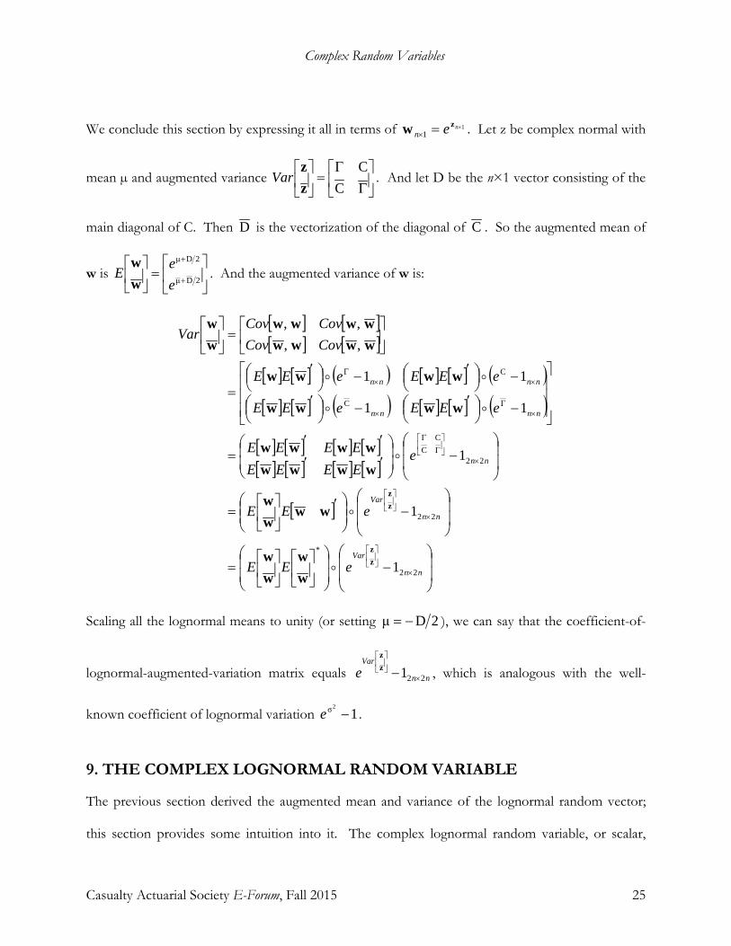
We conclude this section by expressing it all in terms of 11
×=×nen
zw . Let z be complex normal with
mean µ and augmented variance
Γ
Γ=
C
Czz
Var . And let D be the n×1 vector consisting of the
main diagonal of C. Then D is the vectorization of the diagonal of C . So the augmented mean of
w is
=
+
+
2Dμ
2Dμ
ee
Eww
. And the augmented variance of w is:
[ ] [ ][ ] [ ]
[ ] [ ] ( ) [ ] [ ] ( )[ ] [ ] ( ) [ ] [ ] ( )
[ ] [ ] [ ] [ ][ ] [ ] [ ] [ ]
[ ]
−
=
−
′
=
−
′′
′′=
−
′−
′
−
′−
′
=
=
×
×
×
Γ
Γ
×Γ
×
××Γ
nn
Var
nn
Var
nn
nnnn
nnnn
eEE
eEE
eEEEEEEEE
eEEeEE
eEEeEE
CovCovCovCov
Var
22
*
22
22C
C
C
C
1
1
1
11
11
,,,,
zz
zz
ww
ww
wwww
wwwwwwww
wwww
wwww
wwwwwwww
ww
Scaling all the lognormal means to unity (or setting 2Dμ −= ), we can say that the coefficient-of-
lognormal-augmented-variation matrix equals nn
Vare 221 ×
−zz
, which is analogous with the well-
known coefficient of lognormal variation 12σ −e .
9. THE COMPLEX LOGNORMAL RANDOM VARIABLE
The previous section derived the augmented mean and variance of the lognormal random vector;
this section provides some intuition into it. The complex lognormal random variable, or scalar,
Complex Random Variables
Casualty Actuarial Society E-Forum, Fall 2015 26
derives from the real-valued normal bivariate
2
2
τρστρστσ
,00
~ NYX
. Zero is not much of a
restriction; since ( ) ( ) ( )V,0μV,0μVμ, CNCNCN eeee == + , the normal mean affects only the scale of the
lognormal. The variance is written in correlation form, where 1ρ1 ≤≤− . As usual, ∞<< τσ,0 .
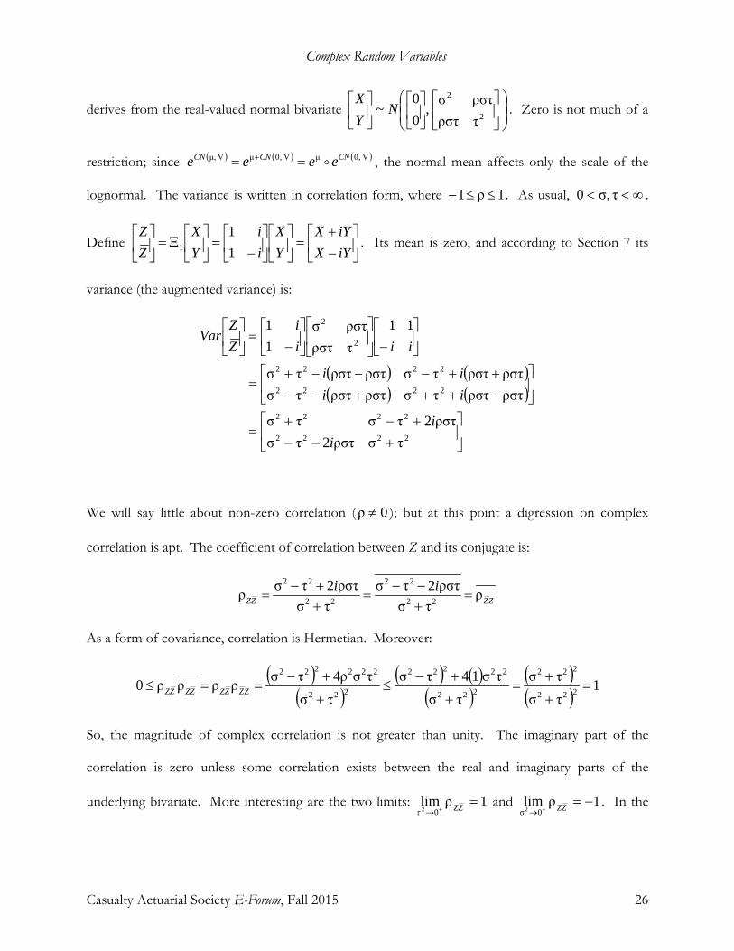
Define
−+
=
−
=
Ξ=
iYXiYX
YX
ii
YX
ZZ
11
1 . Its mean is zero, and according to Section 7 its
variance (the augmented variance) is:
( ) ( )( ) ( )
+−−+−+
=
−+++−−++−−−+
=
−
−
=
2222
2222
2222
2222
2
2
τσρστ2τσρστ2τστσ
ρστρσττσρστρσττσρστρσττσρστρσττσ
11τρστρστσ
11
ii
iiii
iiii
ZZ
Var
We will say little about non-zero correlation ( 0ρ ≠ ); but at this point a digression on complex
correlation is apt. The coefficient of correlation between Z and its conjugate is:
ZZZZii ρ
τσρστ2τσ
τσρστ2τσρ 22
22
22
22
=+−−
=++−
=
As a form of covariance, correlation is Hermetian. Moreover:
( )( )
( ) ( )( )
( )( ) 1
τστσ
τστσ14τσ
τστσρ4τσρρρρ0 222
222
222
22222
222
222222
=+
+=
+
+−≤
+
+−==≤ ZZZZZZZZ
So, the magnitude of complex correlation is not greater than unity. The imaginary part of the
correlation is zero unless some correlation exists between the real and imaginary parts of the
underlying bivariate. More interesting are the two limits: 1ρlim02
=+→ ZZτ
and 1ρlim0σ2
−=+→ ZZ . In the

Complex Random Variables
Casualty Actuarial Society E-Forum, Fall 2015 27
first case, ZZ → in a statistical sense, and the correlation approaches one. In the second case,
ZZ −→ , and the correlation approaches negative one.
Now if ZeW = , by the formulas of Section 8, [ ] ( ) ( ) ρστ2τσ2ρστ2τσ0 2222 ii eeeWE ⋅== −+−+ and
[ ] ( ) ρστ2τσ 22 ieeWE −− ⋅= . And the augmented variance is:
( )( )
( ) ( )[ ]
−⋅−⋅−−=
−−−−=
−−−−
=
−
⋅⋅
⋅⋅=
−
=
−−−−−
−+−−
+−−−
+−+−
+−−
+−+
−−
×
+⋅−−⋅+−+
−−−
−−
−
×
2222222
2222222
2222
222222
2222
222222
2222
2222
2222
22
22
τσ2σρστ2τσρστ4τ22σ
ρστ2τσρστ4τ22στσ2σ
τσρστ2ρστ4τσ
ρστ2ρστ4τστστσ
τσρστ2τσ
ρστ2τστσ
ρστ2
ρστ2τσ
22τσρστ2τσ
ρστ2τστσρστ2τσρστ2τσ
ρστ2τσ
ρστ2τσ
22
*
11
1111
11
1
1
eeeeeeeeee
eeeeeee
eeee
ee
e
eeeeeeeee
eWW
EWW
EWW
Var
ii
ii
ii
ii
i
i
i
i
ii
iii
i
ZZ
Var
In the first case above, as +→ 0τ 2 ,
→
112σ2
eWW
E and ( )
−→
1111
122 σσ ee
WW
Var . Since
the complex part Y becomes probability-limited to its mean of zero, the complex lognormal
degenerates to the real-valued XeW = . The limiting result is oblivious to the underlying correlation
ρ, since WW → .
Complex Random Variables
Casualty Actuarial Society E-Forum, Fall 2015 28
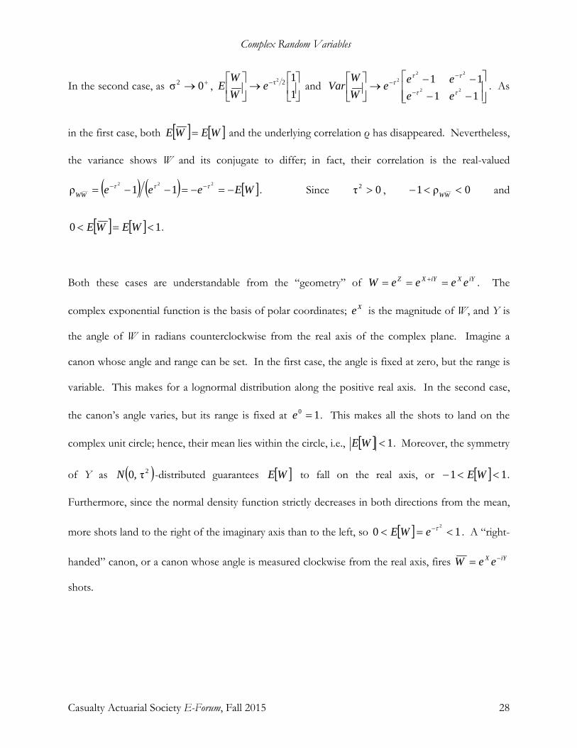
In the second case, as +→ 0σ 2 ,
→
−
112τ2
eWW
E and
−−−−→
−
−−
1111
22
222
ττ
τττ
eeeee
WW
Var . As
in the first case, both [ ] [ ]WEWE = and the underlying correlation ρ has disappeared. Nevertheless,
the variance shows W and its conjugate to differ; in fact, their correlation is the real-valued
( ) ( ) [ ]WEeeeWW −=−=−−= −− 222
11ρ τττ . Since 0τ 2 > , 0ρ1 <<− WW and
[ ] [ ] 10 <=< WEWE .
Both these cases are understandable from the “geometry” of iYXiYXZ eeeeW === + . The
complex exponential function is the basis of polar coordinates; Xe is the magnitude of W, and Y is
the angle of W in radians counterclockwise from the real axis of the complex plane. Imagine a
canon whose angle and range can be set. In the first case, the angle is fixed at zero, but the range is
variable. This makes for a lognormal distribution along the positive real axis. In the second case,
the canon’s angle varies, but its range is fixed at 10 =e . This makes all the shots to land on the
complex unit circle; hence, their mean lies within the circle, i.e., [ ] 1<WE . Moreover, the symmetry
of Y as ( )2τ,0N -distributed guarantees [ ]WE to fall on the real axis, or [ ] 11 <<− WE .
Furthermore, since the normal density function strictly decreases in both directions from the mean,
more shots land to the right of the imaginary axis than to the left, so [ ] 102
<=< −τeWE . A “right-
handed” canon, or a canon whose angle is measured clockwise from the real axis, fires iYX eeW −=
shots.
Complex Random Variables
Casualty Actuarial Society E-Forum, Fall 2015 29
A shot from an unrestricted canon will “almost surely” not land on the real axis.12 If we desire
negative values from the complex lognormal random variable, as a practical matter we must extract
them from its real or complex parts, e.g., ( )WU Re= . One can see in the second case, that as 2τ
grows larger, so too grows larger the probability that 0<U . As ∞→2τ , the probability
approaches one half. In the limit, the shots are uniformly distributed around the complex unit
circle. In this specialized case ( +→ 0σ 2 and ∞→2τ ), the distribution of ( )WU Re= is
( )21
1u
ufU−
=π
, for 11 ≤≤− u .13
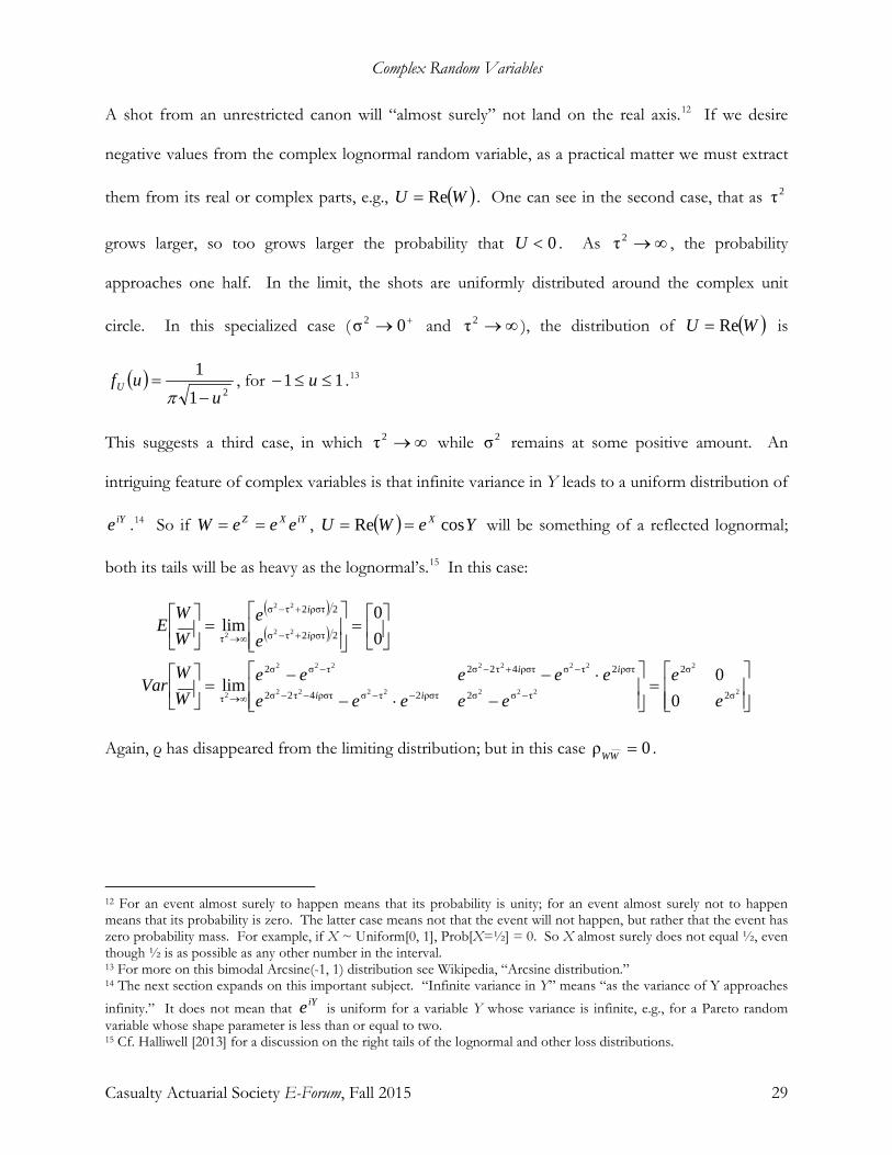
This suggests a third case, in which ∞→2τ while 2σ remains at some positive amount. An
intriguing feature of complex variables is that infinite variance in Y leads to a uniform distribution of
iYe .14 So if iYXZ eeeW == , ( ) YeWU X cosRe == will be something of a reflected lognormal;
both its tails will be as heavy as the lognormal’s.15 In this case:
( )( )
=
−⋅−⋅−−=
=
=
−−−−−
−+−−
∞→
+−
+−
∞→
2
2
2222222
2222222
2
22
22
2
2σ
2σ
τσ2σρστ2τσρστ4τ22σ
ρστ2τσρστ4τ22στσ2σ
τ
2ρστ2τσ
2ρστ2τσ
τ
00lim
00
lim
ee
eeeeeeeeee
WW
Var
ee
WW
E
ii
ii
i
i
Again, ρ has disappeared from the limiting distribution; but in this case 0ρ =WW .
12 For an event almost surely to happen means that its probability is unity; for an event almost surely not to happen means that its probability is zero. The latter case means not that the event will not happen, but rather that the event has zero probability mass. For example, if X ~ Uniform[0, 1], Prob[X=½] = 0. So X almost surely does not equal ½, even though ½ is as possible as any other number in the interval. 13 For more on this bimodal Arcsine(-1, 1) distribution see Wikipedia, “Arcsine distribution.” 14 The next section expands on this important subject. “Infinite variance in Y” means “as the variance of Y approaches
infinity.” It does not mean that iYe is uniform for a variable Y whose variance is infinite, e.g., for a Pareto random variable whose shape parameter is less than or equal to two. 15 Cf. Halliwell [2013] for a discussion on the right tails of the lognormal and other loss distributions.
Complex Random Variables
Casualty Actuarial Society E-Forum, Fall 2015 30
In practical work with ( )WU Re= ,16 the angular part iYe will be more important than the
lognormal range Xe . For example, one who wanted the tendency for the larger magnitudes of
( )WU Re= to be positive might set the mean of Y at 2π− and the correlation ρ to some positive
value. Thus, greater than average values of Y, angling off into quadrants 4 and 1 of the complex
plane, would correlate with larger than average values of X and hence of Xe . Of course,
[ ] 2τ=YVar would have to be small enough that deviations of π± from [ ] 2π−=YE would be
tolerably rare. Equivalently, one could set the mean of Y at 2π and the correlation ρ to some
negative value. As a second example, one who wanted negative values of U to be less frequent than
positive, might set both the mean of Y and ρ to zero, and set the variance of Y so that
[ ]2Prob π>Y is desirably small. Some distributions of U for 22 στ >> are bimodal, as in the
specialized case +→ 0σ 2 and ∞→2τ . But less extreme parameters would result in unimodal
distributions for U over the entire real number line.
10. THE COMPLEX UNIT-CIRCLE RANDOM VARIABLE
In the previous section we claimed that as the variance 2τ of the normal random variable Y
approaches infinity, iYe approaches a uniform distribution over the complex unit circle. The
explanation and justification of this claim in this section prepare for an important implication in the
next.
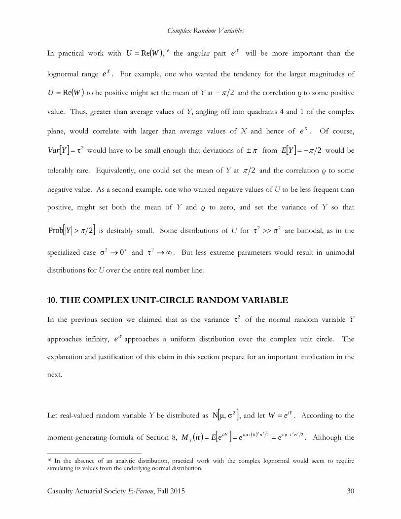
Let real-valued random variable Y be distributed as [ ]2σμ,N , and let iYeW = . According to the
moment-generating-formula of Section 8, ( ) [ ] ( ) 2σμ2σμ 2222 tititititYY eeeEitM −+ === . Although the
16 In the absence of an analytic distribution, practical work with the complex lognormal would seem to require simulating its values from the underlying normal distribution.

Complex Random Variables
Casualty Actuarial Society E-Forum, Fall 2015 31
formula applies to complex values of t, here we’ll restrict it to real values. With ℜ∈t ( )itMY is
known as the characteristic function of real variable Y. And so:
( )
≠=
==== −
∞→
−
∞→∞→ 0if00if1
δlimlimlim 02σ
σ
μ2σμ
σσ
22
2
22
22 tt
eeeitM ttittit
Y
It is noteworthy, and indicative of a uniformity of some sort, that µ drops out of the result.
Next, let real-valued random variable Θ be uniformly distributed over [ ]naa π2, + , where n is a
positive integer; in symbols, [ ]naa π2,U~ +Θ . Then:
( ) [ ]
≠±±=
==
−=
=
=
=
+
+
=
ΘΘ
∫
integralnot if0,2,1if0
0if12
1
2
θ21
2
2θ
2
θ
θ
tntnt
itnee
itne
dn
e
eEitM
itnita
na
a
it
na
a
it
it
π
π
π
π
π
π
Letting n approach infinity, we have:
( )
==
==−
=∞→Θ∞→ 0if0
0if1δ
21limlim 0
2
tt
itneeitM t
itn
n
ita
n π
π
Hence, ( ) ( ) 0σ
δlimlim2 tYn
itMitM ==∞→
Θ∞→. The equality of the limits of the characteristic functions of
the random variables implies the identity of the limits of their distributions; hence, the diffuse
uniform [ ]∞+aa,U is “the same” as the diffuse normal [ ]∞μ,N .17
17 Quotes are around ‘the same’ because the limiting distributions are not proper distributions. The notion of diffuse distributions comes from Venter [1996, pp. 406-410], who shows there how different diffuse distributions result in
Complex Random Variables
Casualty Actuarial Society E-Forum, Fall 2015 32
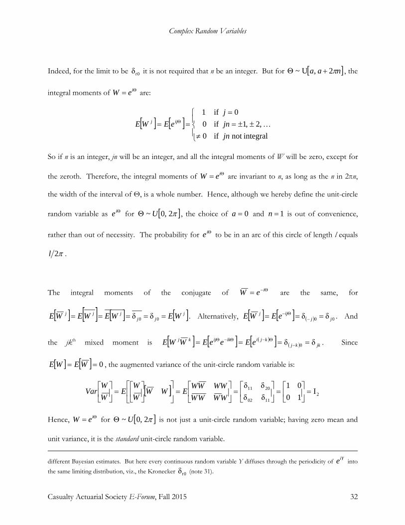
Indeed, for the limit to be 0δt it is not required that n be an integer. But for [ ]naa π2,U~ +Θ , the
integral moments of Θ= ieW are:
[ ] [ ]
≠±±=
=== Θ
integralnot if0,2,1if0
0if1
jnjnj
eEWE ijj
So if n is an integer, jn will be an integer, and all the integral moments of W will be zero, except for
the zeroth. Therefore, the integral moments of Θ= ieW are invariant to n, as long as the n in 2πn,
the width of the interval of Θ, is a whole number. Hence, although we hereby define the unit-circle
random variable as Θie for [ ]π2,0~ UΘ , the choice of 0=a and 1=n is out of convenience,
rather than out of necessity. The probability for Θie to be in an arc of this circle of length l equals
π2l .
The integral moments of the conjugate of Θ−= ieW are the same, for
[ ] [ ] [ ] [ ]jjjjjj WEWEWEWE ===== 00 δδ . Alternatively, [ ] [ ] ( ) 00 δδ jj
ijj eEWE === −Θ− . And
the jkth mixed moment is [ ] [ ] ( )[ ] ( ) jkkjkjiikijkj eEeeEWWE δδ 0 ==== −Θ−Θ−Θ . Since
[ ] [ ] 0== WEWE , the augmented variance of the unit-circle random variable is:
[ ] 21102
2011 I1001
δδδδ
=
=
=
=
=
WWWW
WWWWEWW
WW
EWW
Var
Hence, Θ= ieW for [ ]π2,0~ UΘ is not just a unit-circle random variable; having zero mean and
unit variance, it is the standard unit-circle random variable. different Bayesian estimates. But here every continuous random variable Y diffuses through the periodicity of iYe into the same limiting distribution, viz., the Kronecker 0δt (note 31).
Complex Random Variables
Casualty Actuarial Society E-Forum, Fall 2015 33
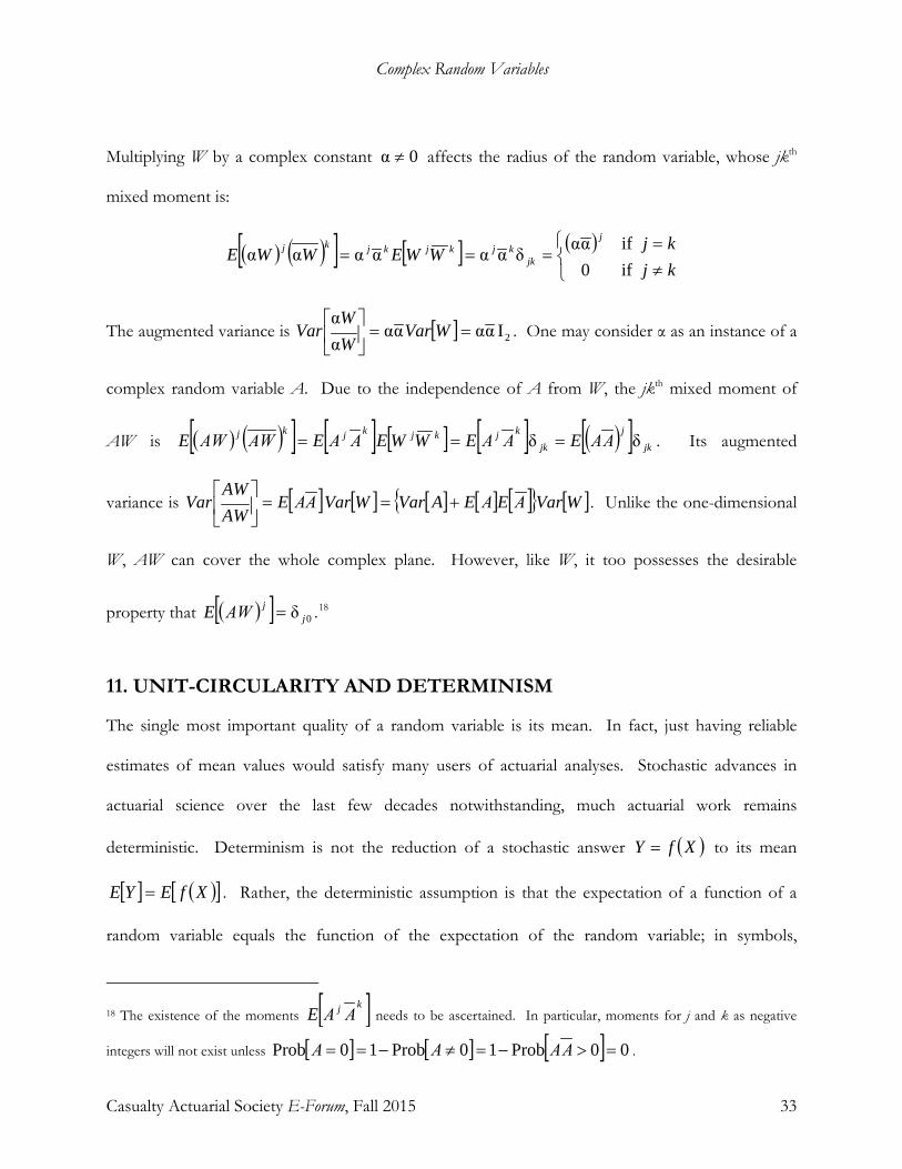
Multiplying W by a complex constant 0α ≠ affects the radius of the random variable, whose jkth
mixed moment is:
( ) ( )[ ] [ ] ( )
≠=
===kjkjWWEWWE
j
jkkjkjkjkj
if0ifααδαααααα
The augmented variance is [ ] 2Iαααααα
==
WVarWW
Var . One may consider α as an instance of a
complex random variable Α. Due to the independence of Α from W, the jkth mixed moment of
ΑW is ( ) ( )[ ] [ ] [ ] [ ] ( )[ ] jkj
jkkjkjkjkj ΑΑEΑΑEWWEΑΑEΑWΑWE δδ === . Its augmented
variance is [ ] [ ] [ ] [ ] [ ]{ } [ ]WVarΑEΑEAVarWVarΑΑEAWAW
Var +==
. Unlike the one-dimensional
W, ΑW can cover the whole complex plane. However, like W, it too possesses the desirable
property that ( )[ ] 0δ jjΑWE = .18
11. UNIT-CIRCULARITY AND DETERMINISM
The single most important quality of a random variable is its mean. In fact, just having reliable
estimates of mean values would satisfy many users of actuarial analyses. Stochastic advances in
actuarial science over the last few decades notwithstanding, much actuarial work remains
deterministic. Determinism is not the reduction of a stochastic answer ( )XfY = to its mean
[ ] ( )[ ]XfEYE = . Rather, the deterministic assumption is that the expectation of a function of a
random variable equals the function of the expectation of the random variable; in symbols,
18 The existence of the moments [ ]kj ΑΑE needs to be ascertained. In particular, moments for j and k as negative
integers will not exist unless [ ] [ ] [ ] 00Prob10Prob10Prob =>−=≠−== ΑΑΑΑ .

Complex Random Variables
Casualty Actuarial Society E-Forum, Fall 2015 34
[ ] ( )[ ] [ ]( )XEfXfEYE == . Because this assumption is true for linear f, it was felt to be a
reasonable or necessary approximation for non-linear f.
Advances in computing hardware and software, as well as increased technical sophistication, have
made determinism more avoidable and less acceptable. However, the complex unit-circular random
variable provides a habitat for the survival of determinism. To see this, let f be analytic over the
domain of complex random variable Z. From Cauchy’s Integral Formula (Havil [2003, Appendix
D.8 and D.9]) it follows that within the domain of Z, f can be expressed as a convergent series
( ) ∑∞
=
+=++=1
010j
jj zaazaazf . Taking the expectation, we have:
( )[ ] [ ]∑∞
=
+=1
0j
jj ZEaaZfE
But if for every positive integer j [ ] [ ] jj ZEZE = , then:
( )[ ] [ ] [ ] [ ]( )ZEfZEaaZEaaZfEj
jj
j
jj =+=+= ∑∑
∞
=
∞
= 10
10
Therefore, determinism conveniently works for analytic functions of random variables whose
moments are powers of their means.
Now a real-valued random variable whose moments are powers of its mean would have the
characteristic function:
( ) [ ] ( ) [ ] ( ) [ ] [ ][ ] ( )itMeXE
jitXE
jiteEitM XE
XitE
j
jj
j
jj
itXX ==+=+== ∑∑
∞
=
∞
= 11 !1
!1
This is the characteristic function of the “deterministic” random variable, i.e., the random variable
whose probability is massed at one point, its mean. So determinism with real-valued random
Complex Random Variables
Casualty Actuarial Society E-Forum, Fall 2015 35
variables requires “deterministic” random variables. But some complex random variables, such as
the unit-circle, have the property [ ] [ ] jj ZEZE = without being deterministic.
In fact, when [ ] [ ] jj ZEZE = , not only is ( )[ ] [ ][ ]ZEfZfE = . For positive integer k, ( )zf k is as
analytic as f itself; hence, ( )[ ] [ ]( )ZEfZfE kk = . So the determinism with these complex random
variables is valid for all moments; nothing is lost.
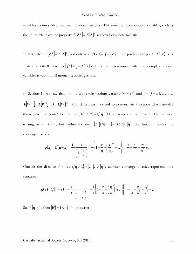
In Section 10 we saw that for the unit-circle random variable Θ= ieW and for ,2,1 ±±=j ,
[ ] [ ] [ ] jjj WEWEWE ===− 0 . Can determinism extend to non-analytic functions which involve
the negative moments? For example, let ( ) ( )zzg −= η1 , for some complex 0η ≠ . The function
is singular at η=z ; but within the disc { } { }η:1η: <=< zzzz the function equals the
convergent series:
( ) ( ) +++=
+
++=
−
⋅=−= 3
2
2
2
ηηη1
ηη1
η1
η1
1η1η1 zzzz
zzzg
Outside the disc, or for { } { }η:1η: >=> zzzz , another convergent series represents the
function:
( ) ( ) −−−−=
+
++−=
−⋅−=−= 3
2
2
2 ηη1ηη11η1
11η1zzzzzz
zz
zzg
So, if 1η > , then η1<=W . In this case:

Complex Random Variables
Casualty Actuarial Society E-Forum, Fall 2015 36
( )[ ]
[ ] [ ]
η1
η0
η0
η1
ηηη1
ηηη1
32
3
2
2
3
2
2
=
+++=
+++=
+++=
WEWE
WWEWgE
However, if 1η < , then η1>=W . So in this case:
( )[ ]
[ ] [ ] [ ]
00η0η0
ηη
ηη1
2
3221
3
2
2
=−⋅−⋅−−=
−−−−=
−−−−=
−−−
WEWEWE
WWWEWgE
Both answers are correct; however, only the first satisfies the deterministic equation
( )[ ] [ ]( ) ( ) η10 === gWEgWgE .
To understand why the answer depends on whether η is inside or outside the complex unit circle, let
us evaluate ( )[ ]WgE directly:
( )[ ] ( )[ ] ( )[ ]π
π
2θ
η1η1η1
2
0θθ
de
eEWEWgE ii ∫
=
Θ
−=−=−=
The next step is to transform from θ into θiez = . So θθθ izddiedz i == , and the line integral
transforms into a contour integral over the unit circle C:
Complex Random Variables
Casualty Actuarial Society E-Forum, Fall 2015 37
( )[ ]
( )
−−
−=
−+=
−
+=
−=
−=
−=
−=
∫∫
∫∫
∫
∫
∫
∫
∫=
CC
CC
C
C
C
C
i
zdz
izdz
i
zdz
izdz
i
dzzzi
zzdz
i
idz
zz
diziz
z
de
WgE
η21
021
η1
η21
21
η1
η1
η11
21
η21
21
η1
2θ
η1
2θ
η12
0θθ
ππ
ππ
π
π
π
π
π
π
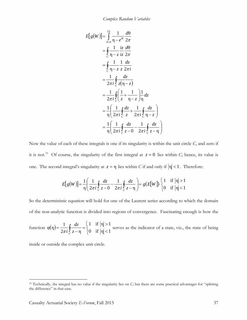
Now the value of each of these integrals is one if its singularity is within the unit circle C, and zero if
it is not.19 Of course, the singularity of the first integral at 0=z lies within C; hence, its value is
one. The second integral’s singularity at η=z lies within C if and only if 1η < . Therefore:
( )[ ] [ ]( )
<>
⋅=
−−
−= ∫∫ 1ηif0
1ηif1η2
102
1η1 WEg
zdz
izdz
iWgE
CC ππ
So the deterministic equation will hold for one of the Laurent series according to which the domain
of the non-analytic function is divided into regions of convergence. Fascinating enough is how the
function ( )
<>
=−
= ∫ 1ηif01ηif1
η21ηφ
C zdz
iπ serves as the indicator of a state, viz., the state of being
inside or outside the complex unit circle.
19 Technically, the integral has no value if the singularity lies on C; but there are some practical advantages for “splitting the difference” in that case.
Complex Random Variables
Casualty Actuarial Society E-Forum, Fall 2015 38
12. THE LINEAR STATISTICAL MODEL
Better known as “regression” models, linear statistical models extend readily into the realm of
complex numbers. A general real-valued form of such models is presented and derived in Halliwell
[1997, Appendix C]:
ΣΣΣΣ
=
+
=
2221
1211
2
1
2
1
2
1
2
1 ,βXX
ee
ee
yy
Var
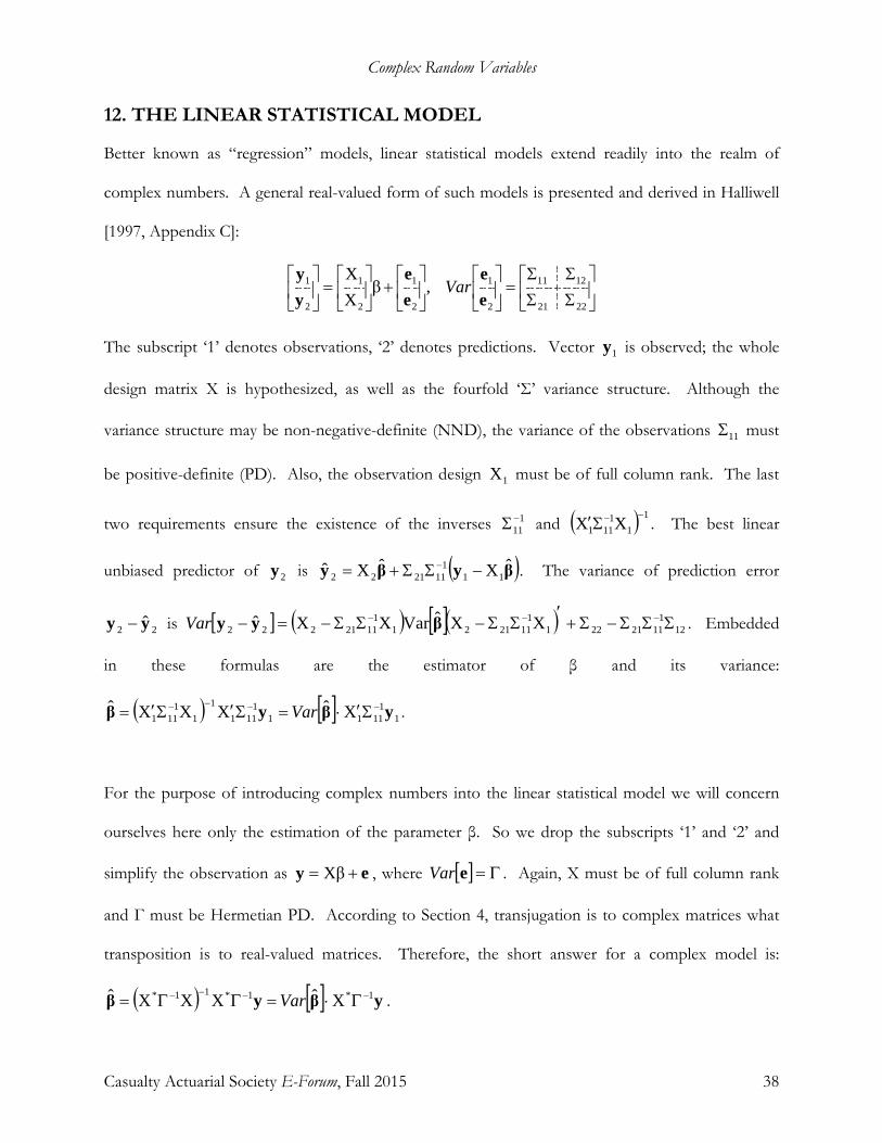
The subscript ‘1’ denotes observations, ‘2’ denotes predictions. Vector 1y is observed; the whole
design matrix X is hypothesized, as well as the fourfold ‘Σ’ variance structure. Although the
variance structure may be non-negative-definite (NND), the variance of the observations 11Σ must
be positive-definite (PD). Also, the observation design 1X must be of full column rank. The last
two requirements ensure the existence of the inverses 111−Σ and ( ) 1
11
111 XX −−Σ′ . The best linear
unbiased predictor of 2y is ( )βyβy ˆXˆXˆ 111
112122 −ΣΣ+= − . The variance of prediction error
22 yy − is [ ] ( ) [ ]( ) 121
11212211
1121211
1121222 XXˆVarXXˆ ΣΣΣ−Σ+′
ΣΣ−ΣΣ−=− −−− βyyVar . Embedded
in these formulas are the estimator of β and its variance:
( ) [ ] 11
11111
1111
11
111 XˆXXXˆ yβyβ −−−− Σ′⋅=Σ′Σ′= Var .
For the purpose of introducing complex numbers into the linear statistical model we will concern
ourselves here only the estimation of the parameter β. So we drop the subscripts ‘1’ and ‘2’ and
simplify the observation as ey += Xβ , where [ ] Γ=eVar . Again, X must be of full column rank
and Γ must be Hermetian PD. According to Section 4, transjugation is to complex matrices what
transposition is to real-valued matrices. Therefore, the short answer for a complex model is:
( ) [ ] yβyβ 1*1*11* XˆXXXˆ −−−− Γ⋅=ΓΓ= Var .
Complex Random Variables
Casualty Actuarial Society E-Forum, Fall 2015 39
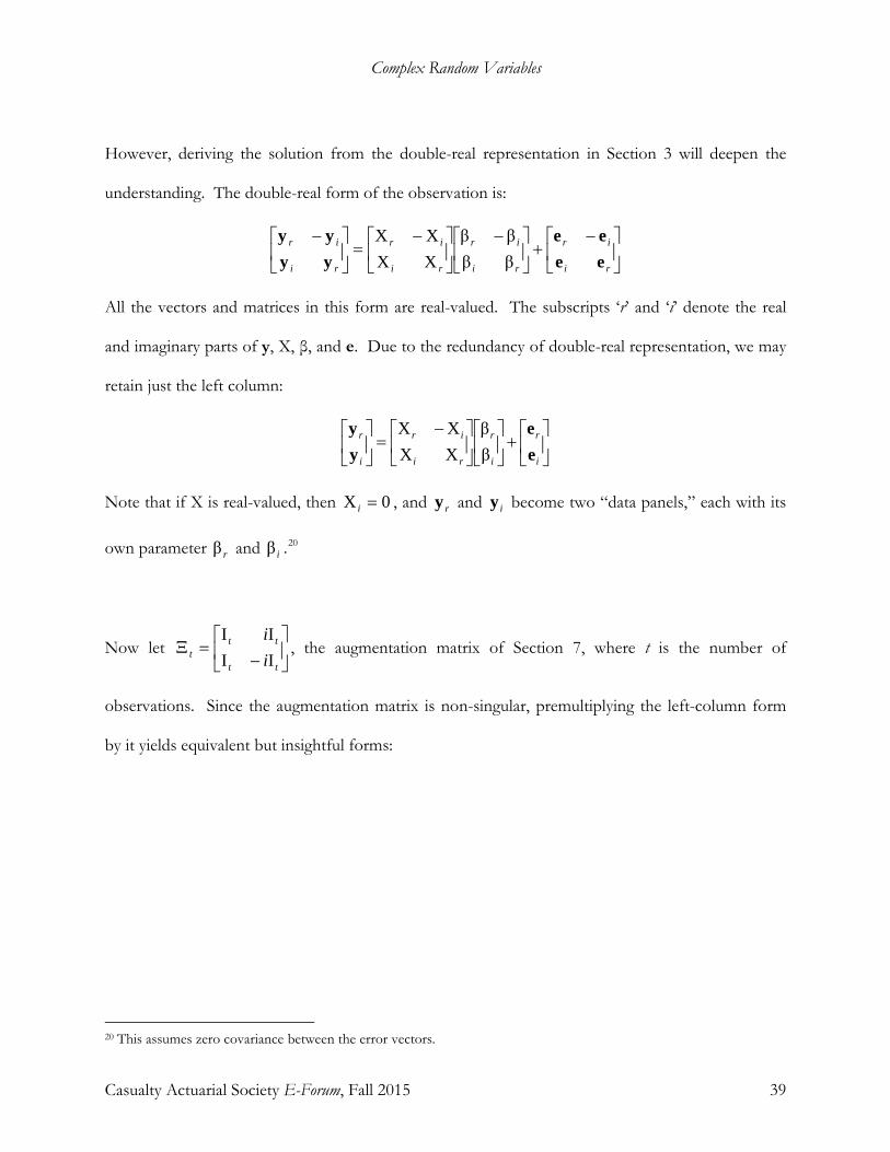
However, deriving the solution from the double-real representation in Section 3 will deepen the
understanding. The double-real form of the observation is:
−+
−
−=
−
ri
ir
ri
ir
ri
ir
ri
ir
eeee
yyyy
ββββ
XXXX
All the vectors and matrices in this form are real-valued. The subscripts ‘r’ and ‘i’ denote the real
and imaginary parts of y, X, β, and e. Due to the redundancy of double-real representation, we may
retain just the left column:
+
−=
i
r
i
r
ri
ir
i
r
ee
yy
ββ
XXXX
Note that if X is real-valued, then 0X =i , and ry and iy become two “data panels,” each with its
own parameter rβ and iβ .20
Now let
−
=Ξtt
ttt i
iIIII
, the augmentation matrix of Section 7, where t is the number of
observations. Since the augmentation matrix is non-singular, premultiplying the left-column form
by it yields equivalent but insightful forms:
20 This assumes zero covariance between the error vectors.
Complex Random Variables
Casualty Actuarial Society E-Forum, Fall 2015 40
+
=
+
=
+
−+
=
+
−
=
−+
+
−−−+−+
=
−+
−
+
−
−
=
−
ee
yy
ee
yy
ee
yy
ee
yy
eeee
yyyy
ee
yy
ββ
X00X
βXXβ
βXβXXβXβ
ββ
XXXX
ββ
XXXXXXXX
IIII
ββ
XXXX
IIII
IIII
ir
ir
i
r
ir
ir
i
r
riir
riir
ir
ir
i
r
tt
tt
i
r
ri
ir
tt
tt
i
r
tt
tt
ii
ii
ii
iiii
ii
ii
ii
ii
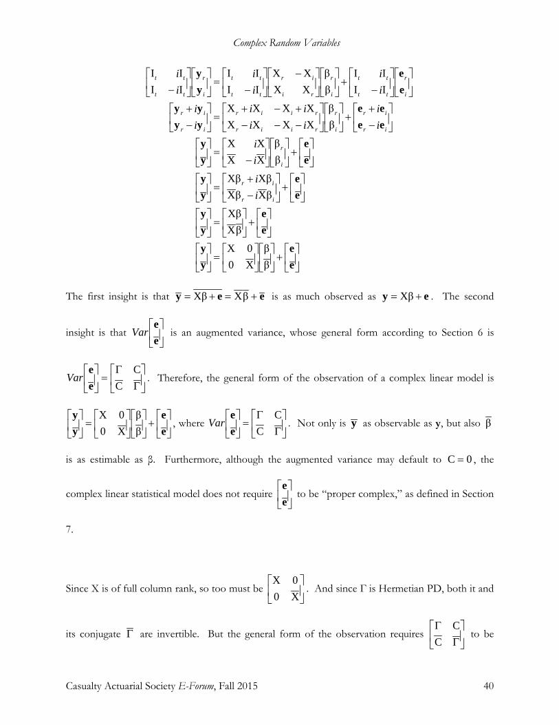
The first insight is that eey +=+= βXXβ is as much observed as ey += Xβ . The second
insight is that
ee
Var is an augmented variance, whose general form according to Section 6 is
Γ
Γ=
C
Cee
Var . Therefore, the general form of the observation of a complex linear model is
+
=
ee
yy
ββ
X00X
, where
Γ
Γ=
C
Cee
Var . Not only is y as observable as y, but also β
is as estimable as β. Furthermore, although the augmented variance may default to 0C = , the
complex linear statistical model does not require
ee
to be “proper complex,” as defined in Section
7.
Since X is of full column rank, so too must be
X00X
. And since Γ is Hermetian PD, both it and
its conjugate Γ are invertible. But the general form of the observation requires
Γ
ΓC
C to be

Complex Random Variables
Casualty Actuarial Society E-Forum, Fall 2015 41
Hermetian PD, hence invertible. A consequence is that both the “determinant” forms CC 1−Γ−Γ
and CC 1−Γ−Γ are Hermetian PD and invertible. With this background it can be shown, and the
reader should verify, that
Η
Η=
Γ
Γ −
KK
CC 1
, where ( ) 11CC −−Γ−Γ=Η and ΗΓ−= − CK 1 . The
important point is that inversion preserves the augmented-variance form.
The solution of the complex linear model
+
=
ee
yy
ββ
X00X
, where
Γ
Γ=
C
Cee
Var , is:
Η′+′+Η
Η′′Η
=
Η
Η
′
Η
Η
′
=
Γ
Γ
Γ
Γ
=
−
−
−−−
yyyy
yy
yy
ββ
XKXKXX
XXXKXXKXXX
KK
X00X
X00X
KK
X00X
CC
X00X
X00X
CC
X00X
ˆˆ
**1**
*1*
1*11*
And 1**
XXXKXXKXXX
ˆˆ −
Η′′Η
=
ββVar , which must exist since it is a quadratic form based on the
Hermetian PD 1
CC −
Γ
Γ and the full column rank
X00X
. Reformulate this as:
Η′+′+Η
=
Η′′Η
yyyy
ββ
XKXKXX
ˆˆ
XXXKXXKXXX ****
The conjugates of the two equations in β and β are the same equations in β and β :
Η′′Η
=
Η′+′+Η
=
Η′′Η
ββ
yyyy
ββ
ˆˆ
XXXKXXKXXX
XKXKXX
ˆ
ˆ
XXXKXXKXXX ******
Complex Random Variables
Casualty Actuarial Society E-Forum, Fall 2015 42
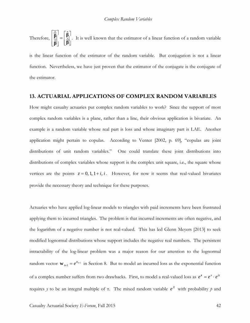
Therefore,
=
ββ
ββ
ˆˆ
ˆ
ˆ. It is well known that the estimator of a linear function of a random variable
is the linear function of the estimator of the random variable. But conjugation is not a linear
function. Nevertheless, we have just proven that the estimator of the conjugate is the conjugate of
the estimator.
13. ACTUARIAL APPLICATIONS OF COMPLEX RANDOM VARIABLES
How might casualty actuaries put complex random variables to work? Since the support of most
complex random variables is a plane, rather than a line, their obvious application is bivariate. An
example is a random variable whose real part is loss and whose imaginary part is LAE. Another
application might pertain to copulas. According to Venter [2002, p. 69], “copulas are joint
distributions of unit random variables.” One could translate these joint distributions into
distributions of complex variables whose support is the complex unit square, i.e., the square whose
vertices are the points iiz ,1,1,0 += . However, for now it seems that real-valued bivariates
provide the necessary theory and technique for these purposes.
Actuaries who have applied log-linear models to triangles with paid increments have been frustrated
applying them to incurred triangles. The problem is that incurred increments are often negative, and
the logarithm of a negative number is not real-valued. This has led Glenn Meyers [2013] to seek
modified lognormal distributions whose support includes the negative real numbers. The persistent
intractability of the log-linear problem was a major reason for our attention to the lognormal
random vector 11
×=×nen
zw in Section 8. But to model an incurred loss as the exponential function
of a complex number suffers from two drawbacks. First, to model a real-valued loss as iyx eee ⋅=z
requires y to be an integral multiple of π. The mixed random variable Xe with probability p and

Complex Random Variables
Casualty Actuarial Society E-Forum, Fall 2015 43
Xe− with probability p−1 is not lognormal. No more suitable are such “denatured” random
variables as ( )ZeRe . Second, one still cannot model the eminently practical value of zero, because
for all z, 0≠ze .21 At present it does not appear that complex random variables will give birth to
useful distributions of real-valued random variables. Even the unit-circle and indicator random
variables of Sections 10 and 11, as interesting as they are in the theory of analytic functions, most
likely will engender no distributions valuable to actuarial work.
The complex version of the linear model in Section 12 showed us that conjugates of observations
are themselves observations and that conjugates of estimators are estimators of conjugates.
Moreover, there we found a use for augmented variance. Nonetheless we are still fairly bound to
our conclusion to Section 3, that one who lacked either the confidence or the software to work with
complex numbers could probably do a work-around with double-real matrices.
So how can actuarial science benefit from complex random variables? The great benefit will come
from new ways of thinking. The first step will be to overcome the habit of picturing a complex
number as half real and half imaginary. Historically, it was only after numbers had expanded from
rational to irrational that the whole set was called “real.” Numbers ultimately are sets; zero is just
the empty set. How real are sets? Regardless of their mathematical reality, they are not physically
real. Complex numbers were deemed “real” because mathematicians needed them for the solution
of polynomial equations. In the nineteenth century this spurred the development of abstract
algebra. At first new ways of thinking amount to differences in degree; at some point many develop
21 If 0=ae for some a, then for all z 00 =⋅=== −−+− azaazaazz eeeee . One who sees that
00lim =⋅=⋅−∞→
iyiyx
xeee might propose to add the ordinate ( ) −∞== xzRe to the complex plane. But not only
is this proposal artificial; it also militates against the standard theory of complex variables, according to which all points infinitely far from zero constitute one and the same point at infinity.
Complex Random Variables
Casualty Actuarial Society E-Forum, Fall 2015 44
into differences in kind. One might argue, “Why study Euclidean geometry? It all derives from a
few axioms.” True, but great theorems (e.g., that the sum of the angles of a triangle is the sum of
two right angles) can be a long way from their axioms. A theorem means more than the course of
its proof; often there are many proofs of a theorem. Furthermore, mathematicians often work
backwards from accepted or desired truths to efficient and elegant sets of axioms. Perhaps the
most wonderful thing about mathematics is its “unreasonable effectiveness in the natural sciences,”
to quote physicist Eugene Wigner. The causality between pure and applied mathematics works in
both directions. Therefore, it is likely that complex random variables and vectors will find their way
into actuarial science. But it will take years, even decades, and technology and education will have to
prepare for it.
14. CONCLUSION
Just as physics divides into different areas, e.g., theoretical, experimental, and applied, so too
actuarial science, though perhaps more concentrated on business application, justifiably has and
needs a theoretical component. Theory and application cross-fertilize each other. In this paper we
have proposed to add complex numbers to the probability and statistics of actuarial theory. With
patience, the technically inclined actuary should be able to understand the theory of complex
random variables delineated herein. In fact, our multivariate approach may even more difficult to
understand than the complex-function theory; but both belong together. Although all complex
matrices and operations were formed from double-real counterparts, we believe that the “sum is
greater than the parts,” i.e., that the assimilation of this theory will lead to higher-order thinking and
creativity. In the sixteenth century the “fiction” of 1−=i allowed mathematicians to solve more
equations. Although at first complex solutions were deemed “extraneous roots,” eventually their
practicality became recognized; so that today complex numbers are essential for science and
Complex Random Variables
Casualty Actuarial Society E-Forum, Fall 2015 45
engineering. Applying complex numbers to probability has lagged; but even now it is part of signal
processing in electrical engineering. Knowing how rapidly science has developed with nuclear
physics, molecular biology, space exploration, and computers, who would dare to bet against the
usefulness of complex random variables to actuarial science by the mid-2030s, when many scientists
and futurists expect nuclear fusion to be harnessed and available for commercial purposes?

Complex Random Variables
Casualty Actuarial Society E-Forum, Fall 2015 46
REFERENCES
[1.] Halliwell, Leigh J., Conjoint Prediction of Paid and Incurred Losses, CAS Forum, Summer 1997, 241-380, www.casact.org/pubs/forum/97sforum/97sf1241.pdf.
[2.] Halliwell, Leigh J., “Classifying the Tails of Loss Distributions,” CAS E-Forum, Spring 2013, Volume 2,
www.casact.org/pubs/forum/13spforumv2/Haliwell.pdf.
[3.] Havil, Julian, Gamma: Exploring Euler’s Constant, Princeton University Press, 2003.
[4.] Healy, M. J. R., Matrices for Statistics, Oxford, Clarendon Press, 1986.
[5.] Hogg, Robert V., and Stuart A. Klugman, Loss Distributions, New York, Wiley, 1984.
[6.] Johnson, Richard A., and Dean Wichern, Applied Multivariate Statistical Analysis (Third Edition), Englewood Cliffs, NJ, Prentice Hall, 1992.
[7.] Judge, George G., Hill, R. C., et al., Introduction to the Theory and Practice of Econometrics (Second Edition), New
York, Wiley, 1988.
[8.] Klugman, Stuart A., et al., Loss Models: From Data to Decisions, New York, Wiley, 1998.
[9.] Meyers, Glenn, “The Skew Normal Distribution and Beyond,” Actuarial Review, May 2013, p. 15, www.casact.org/newsletter/pdfUpload/ar/AR_May2013_1.pdf.
[10.] Million, Elizabeth, The Hadamard Product, 2007, http://buzzard.ups.edu/courses/2007spring/
projects/million-paper.pdf.
[11.] Schneider, Hans, and George Barker, Matrices and Linear Algebra, New York, Dover, 1973.
[12.] Veeravalli, V. V., Proper Complex Random Variables and Vectors, 2006, http://courses.engr. illinois.edu/ece461/handouts/notes6.pdf.
[13.] Venter, G.G., "Credibility," Foundations of Casualty Actuarial Science (Third Edition), Casualty Actuarial Society,
1996.
[14.] Venter, G.G., "Tails of Copulas," PCAS LXXXIX, 2002, 68-113, www.casact.org/pubs/proceed/ proceed02/02068.pdf.
[15.] Weyl, Hermann, The Theory of Groups and Quantum Mechanics, New York, Dover, 1950 (ET by H. P. Robertson
from second German Edition 1930).
[16.] Wikipedia contributors, “Arcsine distribution,” Wikipedia, The Free Encyclopedia, http://en.wikipedia.org/wiki/Arcsine_distribution (accessed October 2014).
[17.] Wikipedia contributors, “Complex normal distribution,” Wikipedia, The Free Encyclopedia,
http://en.wikipedia.org/wiki/Complex_normal_distribution (accessed October 2014).
[18.] Wikipedia contributors, “Complex number,” Wikipedia, The Free Encyclopedia, http://en.wikipedia.org/wiki/Complex_number (accessed October 2014).
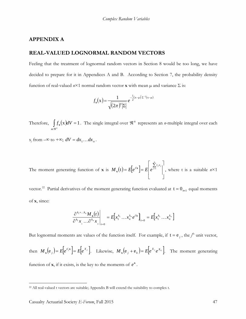
Complex Random Variables
Casualty Actuarial Society E-Forum, Fall 2015 47
APPENDIX A
REAL-VALUED LOGNORMAL RANDOM VECTORS
Feeling that the treatment of lognormal random vectors in Section 8 would be too long, we have
decided to prepare for it in Appendices A and B. According to Section 7, the probability density
function of real-valued n×1 normal random vector x with mean µ and variance Σ is:
( )( )
( ) ( )μxμx21 1
2
1x−Σ′−− −
Σ= ef
nπx
Therefore, ( ) 1x =∫ℜ∈ nx
dVf x . The single integral over nℜ represents an n-multiple integral over each
xj from –∞ to +∞; ndxdxdV 1= .
The moment generating function of x is ( ) [ ]
∑== =′
n
jjj xt
eEeEM 1tt xx , where t is a suitable n×1
vector.22 Partial derivatives of the moment generating function evaluated at 10t ×= n equal moments
of x, since:
( ) [ ] [ ]nn
n
n
nkn
k
t
tkn
k
t
kk
kk
xxEexxExxtM
11
1
1
1
101
0
==∂∂
∂=
′
=
+xx
But lognormal moments are values of the function itself. For example, if jet = , the jth unit vector,
then ( ) [ ] [ ]jj Xj eEeEM == ′ x
xee . Likewise, ( ) [ ]kj XX
kj eeEM =+ eex . The moment generating
function of x, if it exists, is the key to the moments of xe .
22 All real-valued t vectors are suitable; Appendix B will extend the suitability to complex t.
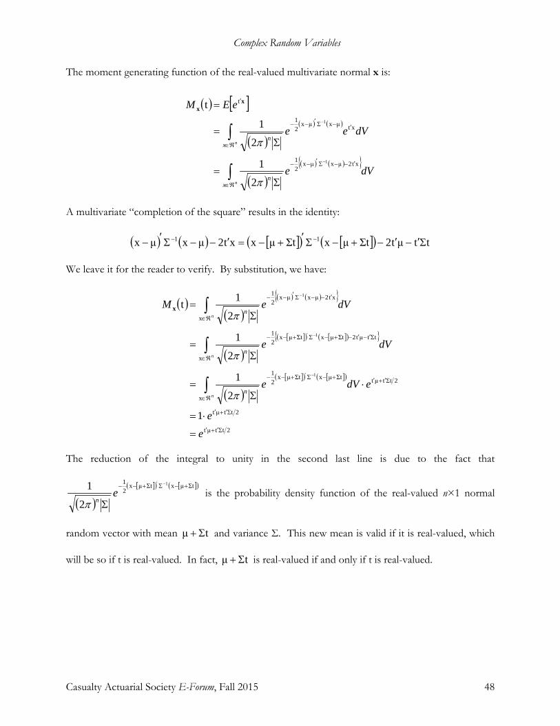
Complex Random Variables
Casualty Actuarial Society E-Forum, Fall 2015 48
The moment generating function of the real-valued multivariate normal x is:
( ) [ ]
( )( ) ( )
( )( ) ( ){ }
dVe
dVee
eEM
n
n
xn
xn
∫
∫
ℜ∈
′−−Σ′−−
ℜ∈
′−Σ′−−
′
−
−
Σ=
Σ=
=
xt2μxμx21
xtμxμx21
t
1
1
2
1
2
1
t
π
π
xx
A multivariate “completion of the square” results in the identity:
( ) ( ) [ ]( ) [ ]( ) ttμt2ΣtμxΣtμxxt2μxμx 11 Σ′−′−+−Σ′+−=′−−Σ′− −−
We leave it for the reader to verify. By substitution, we have:
( )( )
( ) ( ){ }
( )[ ]( ) [ ]( ){ }
( )[ ]( ) [ ]( )
2ttμt
2ttμt
2ttμt
x
ΣtμxΣtμx21
x
ttμt2ΣtμxΣtμx21
x
xt2μxμx21
1
2
1
2
1
2
1t
1
1
1
Σ′+′
Σ′+′
Σ′+′
ℜ∈
+−Σ+−−
ℜ∈
Σ′−′−+−Σ+−−
ℜ∈
′−−Σ′−−
=
⋅=
⋅Σ
=
Σ=
Σ=
∫
∫
∫
−′
−′
−
ee
edVe
dVe
dVeM
n
n
n
n
n
n
π
π
πx
The reduction of the integral to unity in the second last line is due to the fact that
( )[ ]( ) [ ]( )ΣtμxΣtμx
21 1
2
1 +−Σ+−− −′
Σe
nπ is the probability density function of the real-valued n×1 normal
random vector with mean tμ Σ+ and variance Σ. This new mean is valid if it is real-valued, which
will be so if t is real-valued. In fact, tμ Σ+ is real-valued if and only if t is real-valued.
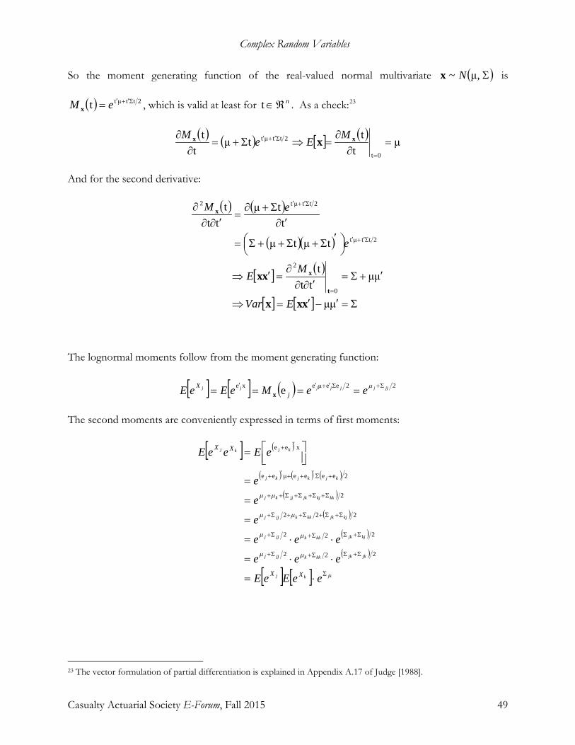
Complex Random Variables
Casualty Actuarial Society E-Forum, Fall 2015 49
So the moment generating function of the real-valued normal multivariate ( )Σ,μ~ Nx is
( ) 2ttμtt Σ′+′= eM x , which is valid at least for nℜ∈t . As a check:23
( ) ( ) [ ] ( )μ
tttμ
tt
0t
2ttμt =∂
∂=⇒Σ+=
∂∂
=
Σ′+′ xx x MEeM
And for the second derivative:
( ) ( )
( )( )
[ ] ( )
[ ] [ ] Σ=′−′=⇒
′+Σ=′∂∂
∂=′⇒
′Σ+Σ++Σ=
′∂Σ+∂
=′∂∂
∂
=
Σ′+′
Σ′+′
μμ
μμtt
t
tμtμ
ttμ
ttt
0
2
2ttμt
2ttμt2
xxx
xxt
x
x
EVar
ME
e
eM
The lognormal moments follow from the moment generating function:
[ ] [ ] ( ) 22eeμexe e jjjjjjjj eeMeEeE jX Σ+Σ′+′′ ==== µ
x
The second moments are conveniently expressed in terms of first moments:
[ ] ( )
( ) ( ) ( )
( )
( )
( )
( )
[ ] [ ] jkkj
jkjkkkkjjj
kjjkkkkjjj
kjjkkkkjjj
kkkjjkjjkj
kjkjkj
kjkj
eeEeE
eee
eee
e
e
e
eEeeE
XX
XX
Σ
Σ+ΣΣ+Σ+
Σ+ΣΣ+Σ+
Σ+Σ+Σ++Σ+
Σ+Σ+Σ+Σ++
+Σ′++′+
′+
⋅=
⋅⋅=
⋅⋅=
=
=
=
=
222
222
222
2
2eeeeμee
xee
µµ
µµ
µµ
µµ
23 The vector formulation of partial differentiation is explained in Appendix A.17 of Judge [1988].

Complex Random Variables
Casualty Actuarial Society E-Forum, Fall 2015 50
So, [ ] [ ] [ ] [ ] [ ] [ ]( )1, −=−= Σ jkkjkjkjkj eeEeEeEeEeeEeeCov XXXXXXXX , which is the multivariate
equivalent of the well-known scalar formula [ ] [ ] [ ] 12σ22 −== eeEeVareCV XXX . Letting [ ]xeE
denote the n×1 vector whose jth element is [ ]jXeE ,24 and [ ]
xeEdiag as its n×n diagonalization,
we have [ ] [ ] { } [ ]
−
= ×
Σ xxx eEdiageeEdiagVar nn1 . Because [ ]
xeEdiag is diagonal in positive
elements (hence, symmetric and PD), [ ]xVar is NND [or PD] if and only if nne ×Σ −1 is NND [or
PD].25 Symmetry is no issue here, because for real-valued matrices, Σ is symmetric if and only if
nne ×Σ −1 is symmetric.
The relation between Σ and nne ×Σ −=Τ 1 is merits a discussion whose result will be clear from a
consideration of 2×2 matrices. Since 22×Σ is symmetric, it is defined in terms of three real numbers:
=Σ
dbba
. Now Σ is NND if and only if 1) 0≥a , 2) 0≥d , and 3) 02 ≥− bad . Σ is PD if and
only if these three conditions are strictly greater than zero. If a or d is zero, by the third condition b
also must be zero.26 Since we are not interested in degenerate random variables, which are
effectively constants, we will require a and d to be positive. With this requirement, Σ is NND if and
24 This would follow naturally from the “elementwise” interpretation of Ae , i.e., that the exponential function of matrix
A is the matrix of the exponential functions of the elements of A. But if A is a square matrix, Ae may have the
“matrix” interpretation ∑∞
=
+1
!AIj
jn j .
25 PD [positive-definite] and NND [non-negative-definite] are defined in Section 4.
26 Since NND matrices represent variances, [ ] [ ][ ] [ ]
=
=
=Σ
dbba
XXCovXXCovXXCovXXCov
XX
Var2212
2111
2
1
,,,,
. The
fact that a or d equals 0 implies that b equals 0 means that a random variable can’t covary with another random variable unless it covaries with itself.
Complex Random Variables
Casualty Actuarial Society E-Forum, Fall 2015 51
only if adb ≤2 , and PD if and only if adb <2 . Since a and d are positive, so too is ad, as well as
the geometric mean ad=γ . So Σ is NND if and only if γγ ≤≤− b , and PD if and only if
γγ <<− b . It is well-known that ( ) ( )dadada ,max2
,min ≤+
≤≤ γ with equality if and only if
da = .
Now the same three conditions determine the definiteness of
−−−−
=−=Τ ×Σ
1111
1 22 db
ba
eeee
e .
Since we required a and d to be positive, both 1−ae and 1−de are positive. This leaves the
definiteness of Τ dependent on the relation between ( )( )11 −− bb ee and ( )( )11 −− da ee . We will
next examine this relation according to the three cases 0=b , 0>b , and 0<b , all of which must
be subject to γγ ≤≤− b .
First, if 0=b , then γγ <<− b and Σ is PD. Furthermore, ( )( ) ( )( )11011 −−<=−− dabb eeee .
Therefore, in this case, the lognormal transformation 221 ×Σ −=Τ→Σ e is from PD to PD. And
zero covariance in the normal pair produces zero covariance in the lognormal pair. In fact, since
zero covariance between normal bivariates implies independence (cf. §2.5.7 of Judge [1988]), the
lognormal bivariates also are independent.
In the second case, 0>b , or more fully, γ≤< b0 . Σ is PD if and only if γ<b . Define the
function ( ) ( )( )xex x 1ln −=ϕ for positive real x (or +ℜ∈x ). A graph will show that the function
strictly increases, i.e., ( ) ( )21 xx ϕϕ < if and only if 21 xx < . Moreover, the function is concave
upward. This means that the line segment between points ( )( )11 , xx ϕ and ( )( )22 , xx ϕ lies above
Complex Random Variables
Casualty Actuarial Society E-Forum, Fall 2015 52
the curve ( )xϕ for intermediate values of x. In particular, ( ) ( )
+
≥+
221121 xxxx
ϕϕϕ
.
Equivalently, for all +ℜ∈21 , xx , ( ) ( )2111
22 xxxx
ϕϕϕ +≤
+
with equality if and only if 21 xx = .
Therefore, since a and d are positive, ( ) ( )dada ϕϕϕ +≤
+
22 . And since
20 daad +
≤=< γ ,
( ) ( ) ( )dada ϕϕϕγϕ +≤
+
≤2
22 . So ( ) ( ) ( )da ϕϕγϕ +≤2 with equality if and only if da = .
Furthermore, since in this case γ≤< b0 , ( ) ( ) ( ) ( )dab ϕϕγϕϕ +≤≤ 22 . Hence,
( ) ( ) ( )dab ϕϕϕ +≤2 . The equality prevails if and only if dab === γ , or if and only if dba == .
If dba == then Σ is not PD; otherwise Σ is PD. Hence:
( ) ( ) ( )
−+
−=+≤=
−d
ea
edabb
e dab 1ln1ln21ln2 ϕϕϕ
The inequality is preserved by exponentiation:
−
−≤
−d
ea
eb
e dab 1112
This leads at last to the inequality:
( ) ( )( ) ( )( ) ( )( )111111111222
22−−⋅≤−−
=−−≤
−=− dadada
bb eeeebee
adb
bebe
γ
Therefore, in this case ( ) ( )( )111 2−−≤− dab eee with equality if and only if dba == . This means
that if 0>b , the lognormal transformation 221 ×Σ −=Τ→Σ e is from NND to NND. But Τ is
NND only if ( ) ( )( )111 2−−=− dab eee , or only if dba == . Otherwise, Τ is PD. So, when
0>b , 221 ×Σ −=Τ e is PD except when all four elements of Σ have the same positive value. Even
Complex Random Variables
Casualty Actuarial Society E-Forum, Fall 2015 53
the NND matrix
=Σ
dadada log-transforms into a PD matrix, unless da = . So all PD and
most NND normal variances transform into PD lognormal variances. A NND lognormal variance
indicates that at least one element of the normal random vector is duplicated.
In the third and final case, 0<b , or more fully, 0<≤− bγ . This is equivalent to γ≤−< b0 , or
to the second case with b− . In that case, ( ) ( )( )111 2−−≤−− dab eee with equality if and only if
dba =−= . But from this, as well as from the fact that 10 022 <<< ⋅ee b , it follows:
( ) ( ) ( ) ( )( ) ( )( )11111111 222222−−⋅<−−≤−=−=− −− dadabbbbbb eeeeeeeeee
So in this case the inequality is strict: ( ) ( )( )111 2−−<− dab eee , and Τ is PD. Therefore, if 0<b ,
the lognormal transform 221 ×Σ −=Τ→Σ e is PD, even if Σ is NND.
To summarize, the lognormal transformation 221 ×Σ −=Τ→Σ e is PD if Σ is PD. Even when Σ is
not PD, but merely NND, Τ is almost always PD. Only when Σ is so NND as to conceal a
random-variable duplication is its lognormal transformation NND.
The Hadamard (elementwise) product and Schur’s product theorem allow for an understanding of
the general lognormal transformation nne ×Σ −=Τ→Σ 1 . Denoting the elementwise nth power of Σ
as
factorsn
n ΣΣ=Σ , we can express elementwise exponentiation as ∑∞
=
Σ Σ=0
!j
j je . So
∑∞
=×
Σ Σ=−=Τ1
!1j
jnn je . According to Schur’s theorem (§3 of Million [2007]), the Hadamard
Complex Random Variables
Casualty Actuarial Society E-Forum, Fall 2015 54
product of two NND matrices is NND.27 Since Σ is NND, its powers jΣ are NND, as well as the
terms !jjΣ . Being the sum of a countable number of NND matrices, Τ also must be NND.28
But if just one of the terms of the sum is PD, the sum itself must be PD. Therefore, if Σ is PD,
then Τ also is PD.
Now the kernel of m×n matrix A is the set of all nℜ∈x such that 0Ax = , or
( ) { }0Ax:xA ==ker . The kernel is a linear subspace of nℜ and its dimensionality is ( )Arankn − .
By the Cholesky decomposition the NND matrix U can be factored as nnnn ×× ′= WWU . The
quadratic form in U is ( ) ( )WxWxWxWxUxx ′=′′=′ . If 0Uxx =′ , then 10Wx ×= n , and
11 00WWxWUx ×× =′=′= nn . Conversely, if 10Ux ×= n , then 0Uxx =′ . So the kernel of NND
matrix U is precisely the solution set of 0Uxx =′ , i.e., 0Uxx =′ if and only if ( )Ukerx∈ .
Therefore, the kernel of ∑∞
=
Σ=Τ1
!j
j j is the intersection of the kernels of jΣ , or
( ) ( ) ∞
=
Σ=Τ1j
jkerker . It is possible for this intersection to be of dimension zero, i.e., for it to equal
{ }10 ×n , even though the kernel of no jΣ is. Because of the accumulation of intersections in
∑∞→
=
Σk
j
j j1
! , the lognormal transformation of NND matrix Σ tends to be “more PD” than Σ itself.
27 Appendix C provides a proof of this theorem.
28 For the quadratic form of a sum equals the sum of the quadratic forms: xUxxUx ∑∑ ′=
′k
kk
k . In fact, if the
coefficients aj are non-negative, then ∑∞
=
Σ1j
jja is NND, provided that the sum converges, as Σe does.
Complex Random Variables
Casualty Actuarial Society E-Forum, Fall 2015 55
We showed above that if Σ is PD, then nne ×Σ −=Τ 1 is PD. But even if Σ is NND, Τ will be PD,
unless Σ contains a 2×2 subvariance
ΣΣΣΣ
kkkj
jkjj whose four elements are all equal.
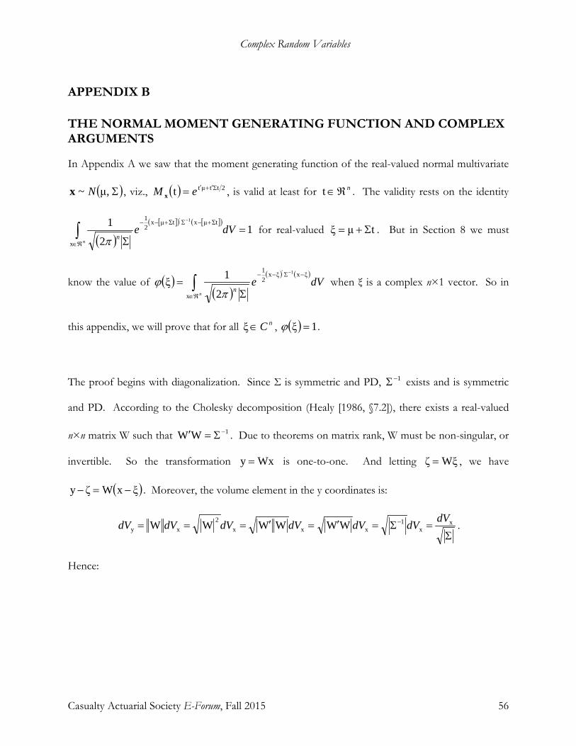
Complex Random Variables
Casualty Actuarial Society E-Forum, Fall 2015 56
APPENDIX B
THE NORMAL MOMENT GENERATING FUNCTION AND COMPLEX ARGUMENTS
In Appendix A we saw that the moment generating function of the real-valued normal multivariate
( )Σ,μ~ Nx , viz., ( ) 2ttμtt Σ′+′= eM x , is valid at least for nℜ∈t . The validity rests on the identity
( )[ ]( ) [ ]( )
12
1
x
ΣtμxΣtμx21 1
=Σ
∫ℜ∈
+−Σ+−− −′
dVen
nπ for real-valued tμξ Σ+= . But in Section 8 we must
know the value of ( )( )
( ) ( )dVe
nn∫
ℜ∈
−Σ−− −′
Σ=
x
ξxξx21 1
2
1ξπ
ϕ when ξ is a complex n×1 vector. So in
this appendix, we will prove that for all nC∈ξ , ( ) 1ξ =ϕ .
The proof begins with diagonalization. Since Σ is symmetric and PD, 1−Σ exists and is symmetric
and PD. According to the Cholesky decomposition (Healy [1986, §7.2]), there exists a real-valued
n×n matrix W such that 1WW −Σ=′ . Due to theorems on matrix rank, W must be non-singular, or
invertible. So the transformation Wxy = is one-to-one. And letting Wξζ = , we have
( )ξxWζy −=− . Moreover, the volume element in the y coordinates is:
Σ=Σ=′=′=== − x
x1
xxx2
xy WWWWWW dVdVdVdVdVdVdV .
Hence:

Complex Random Variables
Casualty Actuarial Society E-Forum, Fall 2015 57
( )( )
( ) ( )
( )( ) ( )
( )( )[ ] ( )[ ]
( )( ) ( )
( )
( )
( )
( )
( )∏
∏ ∫
∫ ∏
∫
∫
∫
∫
∫
=
=
∞
−∞=
−−
ℜ∈ =
−−
ℜ∈
−−
ℜ∈
−′−−
ℜ∈
−′−−
ℜ∈
−′−−
ℜ∈
−Σ−−
=
∑=
∑=
∑=
=
Σ=
Σ=
Σ=
=
=
=
′
−′
n
jj
n
jj
n
j
n
n
n
n
n
j
n
jjj
n
n
jjj
n
n
jjj
n
n
n
n
de
dVe
dVe
dVe
dVe
dVe
dVe
1
1 y
ζy21
y 1
ζy21
y
ζy21
yy
ζyζy21
x
x
ξxWξxW21
xx
ξxWWξx21
x
ξxξx21
ζψ
y21
21
2
1
2
1
2
1
2
1
2
1ξ
1
2
1
2
1
2
1
π
π
π
π
π
π
πϕ
In the last line ( ) ( )∫=
−−
+∞→−∞→
=b
ax
x
ba
dxe2ζ
21
21ζψ lim π
. Obviously, if ζ is real-valued, ( ) 1ζψ = . So the
issue of the value of a moment generating function of a complex variable resolves into the issue of
the “total probability” of a unit-variance normal random variable with a complex mean.29
To evaluate ( )ζψ requires some complex analysis with contour integrals. First, consider the
standard-normal density function with a complex argument: ( ) 2
2
21 z
ezf−
=π
. By function-
composition rules, since both 2z and the exponential function are “entire” functions (i.e., analytic
29 We deliberately put ‘total probability’ in quotes because the probability density function with complex ζ is not proper; it may produce negative and even complex values for probability densities.
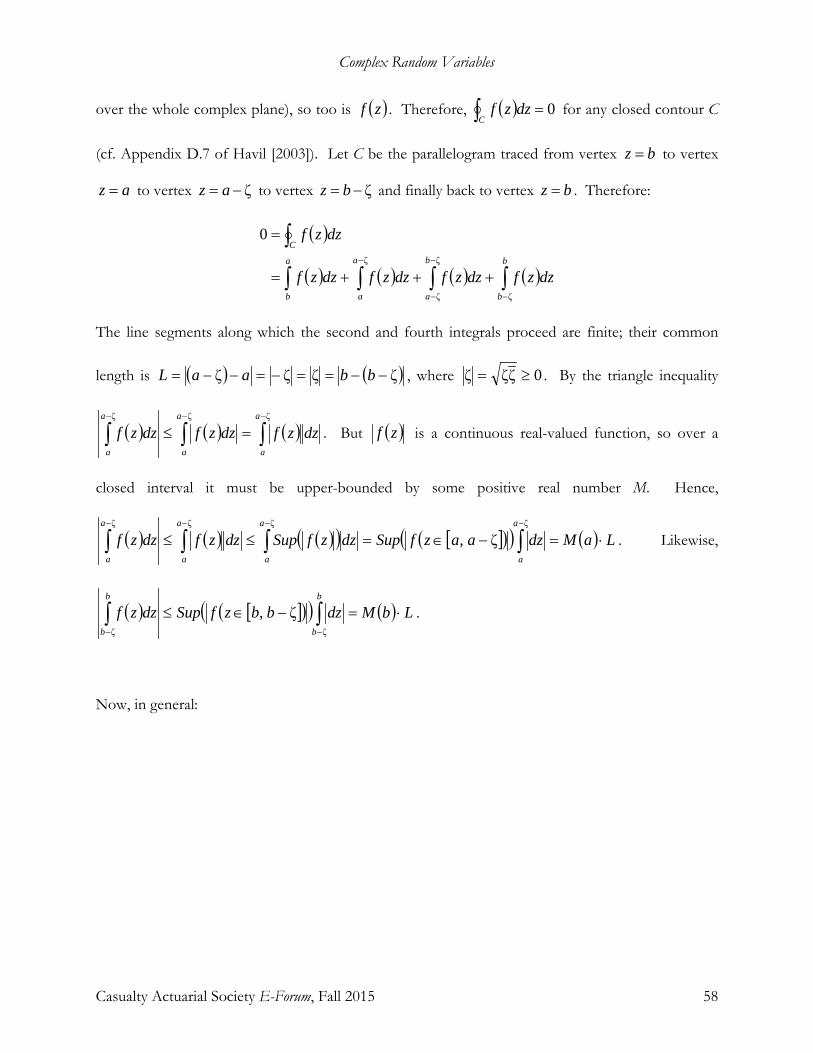
Complex Random Variables
Casualty Actuarial Society E-Forum, Fall 2015 58
over the whole complex plane), so too is ( )zf . Therefore, ( ) 0=∫C dzzf for any closed contour C
(cf. Appendix D.7 of Havil [2003]). Let C be the parallelogram traced from vertex bz = to vertex
az = to vertex ζ−= az to vertex ζ−= bz and finally back to vertex bz = . Therefore:
( )
( ) ( ) ( ) ( )∫∫∫∫
∫
−
−
−
−
+++=
=
b
b
b
a
a
a
a
b
C
dzzfdzzfdzzfdzzf
dzzf
ζ
ζ
ζ
ζ
0
The line segments along which the second and fourth integrals proceed are finite; their common
length is ( ) ( )ζζζζ −−==−=−−= bbaaL , where 0ζζζ ≥= . By the triangle inequality
( ) ( ) ( ) dzzfdzzfdzzfa
a
a
a
a
a∫∫∫−−−
=≤ζζζ
. But ( )zf is a continuous real-valued function, so over a
closed interval it must be upper-bounded by some positive real number M. Hence,
( ) ( ) ( )( ) [ ]( )( ) ( ) LaMdzaazfSupdzzfSupdzzfdzzfa
a
a
a
a
a
a
a
⋅=−∈=≤≤ ∫∫∫∫−−−− ζζζζ
ζ, . Likewise,
( ) [ ]( )( ) ( ) LbMdzbbzfSupdzzfb
b
b
b
⋅=−∈≤ ∫∫−− ζζ
ζ, .
Now, in general:
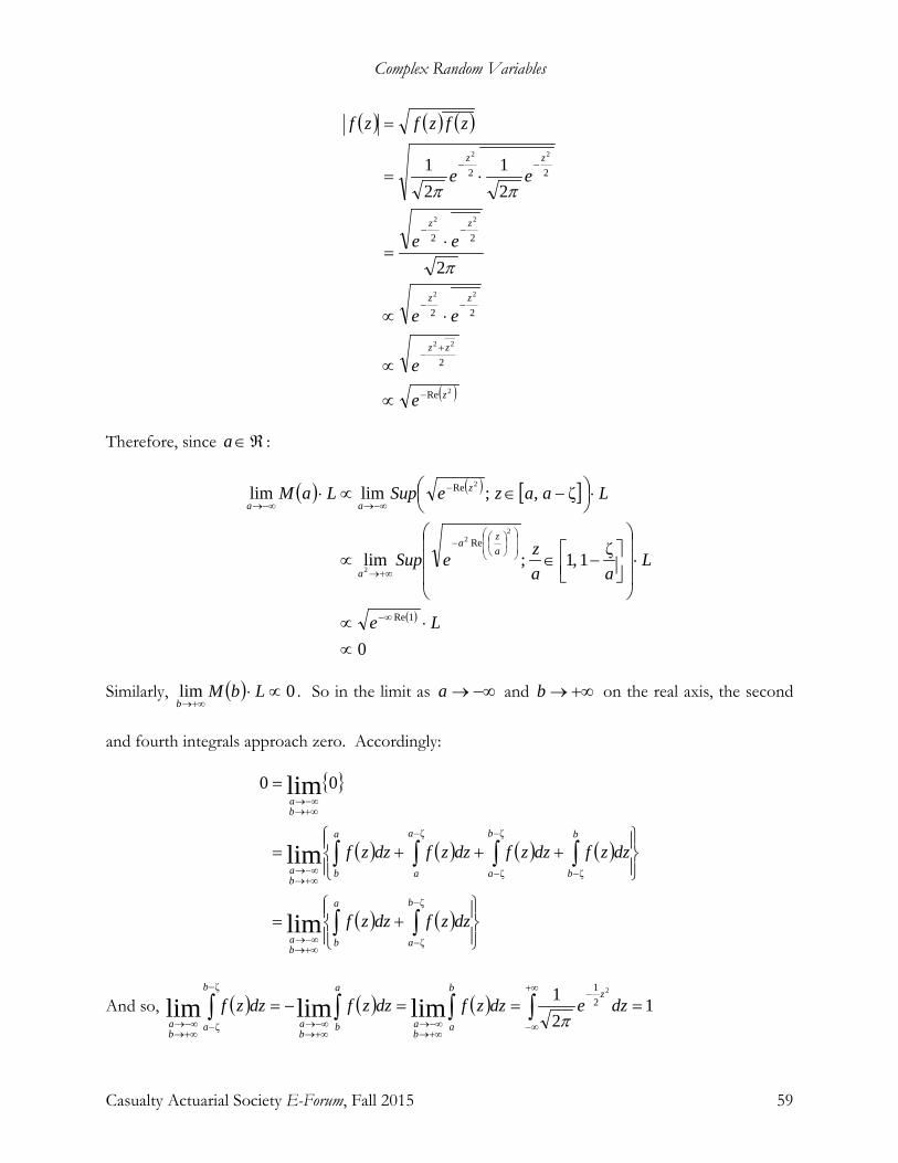
Complex Random Variables
Casualty Actuarial Society E-Forum, Fall 2015 59
( ) ( ) ( )
( )2
22
22
22
22
Re
2
22
22
22
2
21
21
z
zz
zz
zz
zz
e
e
ee
ee
ee
zfzfzf
−
+−
−−
−−
−−
∝
∝
⋅∝
⋅=
⋅=
=
π
ππ
Therefore, since ℜ∈a :
( ) ( ) [ ]
( )
0
ζ1,1;lim
ζ,;limlim
1Re
Re
Re
22
2
2
∝⋅∝
⋅
−∈∝
⋅
−∈∝⋅
∞−
−
+∞→
−
−∞→−∞→
Le
Laa
zeSup
LaazeSupLaM
aza
a
z
aa
Similarly, ( ) 0lim ∝⋅+∞→
LbMb
. So in the limit as −∞→a and +∞→b on the real axis, the second
and fourth integrals approach zero. Accordingly:
{ }
( ) ( ) ( ) ( )
( ) ( )
+=
+++=
=
∫∫
∫∫∫∫
−
−+∞→−∞→
−
−
−
−
+∞→−∞→
+∞→−∞→
ζ
ζ
ζ
ζ
ζ
ζ
lim
lim
lim 00
b
a
a
bba
b
b
b
a
a
a
a
bba
ba
dzzfdzzf
dzzfdzzfdzzfdzzf
And so, ( ) ( ) ( ) 121 2
21ζ
ζlimlimlim ===−= ∫∫∫∫
+∞
∞−
−
+∞→−∞→
+∞→−∞→
−
−+∞→−∞→
dzedzzfdzzfdzzfzb
aba
a
bba
b
aba π

Complex Random Variables
Casualty Actuarial Society E-Forum, Fall 2015 60
So, at length:
( ) ( )
( )( ) ( )
( )
( )
1
21
ζ21
ζ21
21ζψ
ζ
ζ
ζ
ζ
21
ζ
ζ
21
ζζ21
ζ21
lim
lim
lim
lim
lim
2
2
2
2
=
=
=
+=
+=
=
∫
∫
∫
∫
∫
−
−=+∞→−∞→
−
−=
−
+∞→−∞→
−
−=
−
+∞→−∞→
=
−+−
+∞→−∞→
=
−−
+∞→−∞→
b
azba
b
az
z
ba
b
az
z
ba
b
ax
z
ba
b
ax
x
ba
dzzf
dze
zde
zde
dxe
π
π
π
π
So, working backwards, what we proved for one dimension, viz., ( ) ( )1
21ζψ
2ζ21
== ∫+∞
−∞=
−−
x
xdxe
π,
applies n-dimensionally: for all nC∈ξ , ( )( )
( ) ( )1
2
1ξx
ξxξx21 1
=Σ
= ∫ℜ∈
−Σ−− −′
dVen
nπϕ . Therefore, even
for complex t, ( ) 2ttμtt Σ′+′= eM x . Complex values are allowable as arguments in the moment
generating function of a real-valued normal vector. This result is critical to Section 8.
Though we believe the contour-integral proof above to be worthwhile for its instructional value, a
simple proof comes from the powerful theorem of analytic continuation (cf. Appendix D.12 of
Havel [2003]). This theorem concerns two functions that are analytic within a common domain. If
the functions are equal over any smooth curve within the domain, no matter how short,30 then they
30 The length of the curve must be positive; equality at single points, or punctuated equality, does not qualify.
Complex Random Variables
Casualty Actuarial Society E-Forum, Fall 2015 61
are equal over all the domain. Now ( ) ( )∫=
−−
+∞→−∞→
=b
ax
x
ba
dxe2ζ
21
21ζψ lim π
is analytic over all the complex
plane. And for all real-valued ζ, ( ) 1ζψ = . So ( )ζψ and ( ) 1ζ =f are two functions analytic over the
complex plane and identical on the real axis. Therefore, by analytic continuation ( )ζψ must equal
one for all complex ζ. Analytic continuation is analogous with the theorem in real analysis that two
smooth functions equal over any interval are equal everywhere. Analytic continuation derives from
the fact that a complex derivative is the same in all directions. It is mistaken to regard the real and
imaginary parts of the derivative as partial derivatives, as if they applied respectively to the real and
imaginary axes of the independent variable. Rather, the whole derivative applies in every direction.
Complex Random Variables
Casualty Actuarial Society E-Forum, Fall 2015 62
APPENDIX C
EIGEN-DECOMPOSITION AND SCHUR’S PRODUCT THEOREM
Appendix A quoted Schur’s Product Theorem, viz., that the Hadamard product of non-negative-
definite (NND) matrices is NND. Million [2007] proves it as Theorem 3.4; however, we believe our
proof in this appendix to be simpler; moreover, it affords a review of eigen-decomposition. Those
familiar with eigen-decomposition may skip to the last paragraph.
Let Γ be an n×n Hermetian NND matrix. As explained in Section 4, ‘Hermetian’ means that
*Γ=Γ ; ‘NND’ means that for every complex n×n vector z (or nC∈z ), 0zz* ≥Γ . Positive
definiteness [PD] is a stricter condition, in which 0zz* =Γ if and only if 10z ×= n .
Complex scalar λ and non-zero vector ν form an “eigenvalue-eigenvector” pair of Γ, if λνν =Γ .
Since 10ν ×= n is excluded as a trivial solution, vector ν can be scaled to unity, or 1νν* = . But
λνν =Γ if and only if ( ) 10νλI ×=−Γ nn . If nλI−Γ is non-singular, or invertible, then:
( ) ( ) ( ) 1111 00λIνλIλIνIν ××−− =−Γ=−Γ−Γ== nnnnnn
Hence, allowable eigenvectors require for nλI−Γ to be singular, or for its determinant nλI−Γ to
be zero. Since the determinant is an nth-degree equation (with complex coefficients based on the
elements of Γ) in λ, it has n root values of λ, not necessarily distinct. So the determinant can be
factored as ( ) ( ) ( )nnf λλλλλIλ 1 −−=−Γ= . Since ( ) 0Iλλ =−Γ= njjf , there exist non-
zero solutions to ( ) 10νλI ×=−Γ nn . So for every eigenvalue there is a non-zero eigenvector, even a
non-zero eigenvector of unit magnitude.
Complex Random Variables
Casualty Actuarial Society E-Forum, Fall 2015 63
The first important result is that the eigenvalues of Γ are real-valued and non-negative. Consider the
jth eigenvalue-eigenvector pair, which satisfies the equation jjj νλν =Γ . Therefore,
jjjjj ννλνν ** =Γ . Since Γ is NND, jj νν*Γ is real-valued and non-negative. Also, jj νν* is real-
valued and positive. Therefore, their quotient λj is a real-valued and non-negative scalar.
Furthermore, if Γ is PD, jj νν*Γ is positive, as well as λj.
The second important result is that eigenvectors paired with unequal eigenvalues are orthogonal.
Let the two unequal eigenvalues be kj λλ ≠ . Because the eigenvalues are real-valued, jj λλ = . The
eigenvector equations are jjj νλν =Γ and kkk νλν =Γ . The following string of equations relies on
Γ’s being Hermetian (so *Γ=Γ ):
( )
( )( )
0
νννν
νννν
νννν
ννλννλ
ννλννλ
ννλννλννλλ
**
***
***
***
**
***
=
Γ−Γ=
Γ−Γ=
Γ−Γ=
−=
−=
−=−
kjkj
kjkj
kjjk
kjkjkj
kjkkjj
kjkkjjkjkj
Because 0λλ ≠− kj , the eigenvectors must be orthogonal, or 0νν* =kj . If all the eigenvectors are
distinct, the eigenvectors form an orthogonal basis of nC . But even if not, the kernel of each
eigenvalue, or ( ) { }zλz:zIλ jn
nj Cker =Γ∈=−Γ is a linear subspace of nC whose rank or
dimensionality equals the multiplicity of the root λj in the characteristic equation ( ) nf λIλ −Γ= .
This means that the number of mutually orthogonal eigenvectors paired with an eigenvalue equals
Complex Random Variables
Casualty Actuarial Society E-Forum, Fall 2015 64
how many times that eigenvalue is a root of its characteristic equation. Consequently, there exist n
eigenvalue-eigenvector pairs ( )jj ν,λ such that jjj νλν =Γ and ijkj δνν* = .31
Now, define W as the partitioned matrix [ ]nnn ννW 1 =× . The jkth element of W*W equals
ijkj δνν* = ; hence, nIWW* = . A matrix whose transjugate is its inverse is called “unitary,” as is
W.32 Furthermore, define Λ as the n×n diagonal matrix whose jjth element is λj. Then:
[ ] [ ] [ ] [ ] Λ=
==ΓΓ=Γ=Γ W
λ
λνννλνλννννW
1
11111
n
nnnnn
And so, **n WWWWI Λ=Γ=Γ=Γ , and Γ is said to be “diagonalized.” Thus have we shown,
assuming the theory of equations, 33 the third important result, viz., that every NND Hermetian
matrix can be diagonalized. Other matrices can be diagonalized; the NND [or PD] consists in the
fact that all the eigenvalues of this diagonalization are non-negative [or positive].
The fourth and final “eigen” result relies on the identity jj eνW* = , which just extracts the jth
columns of each side of nIWW* = . As in Appendix A, je is the jth unit vector. Therefore:
31 The Kronecker delta, ijδ , is the function ( )0,1,IF ji = . 32 To be precise, at this point W* is only the left-inverse of W. But by matrix-rank theorems, the rank of W equals n, so W has a unique full inverse -1W . Then ( ) ( ) 111*1*** WWIWWWWWWIWW --
n--
n ===== .
33 The theory of equations guarantees the existence of the roots of the nth-degree equation ( ) .λIλ nf −Γ= Appendix D.9 of Havel [2003] contains a quick and lucid proof of this, the fundamental theorem of algebra.
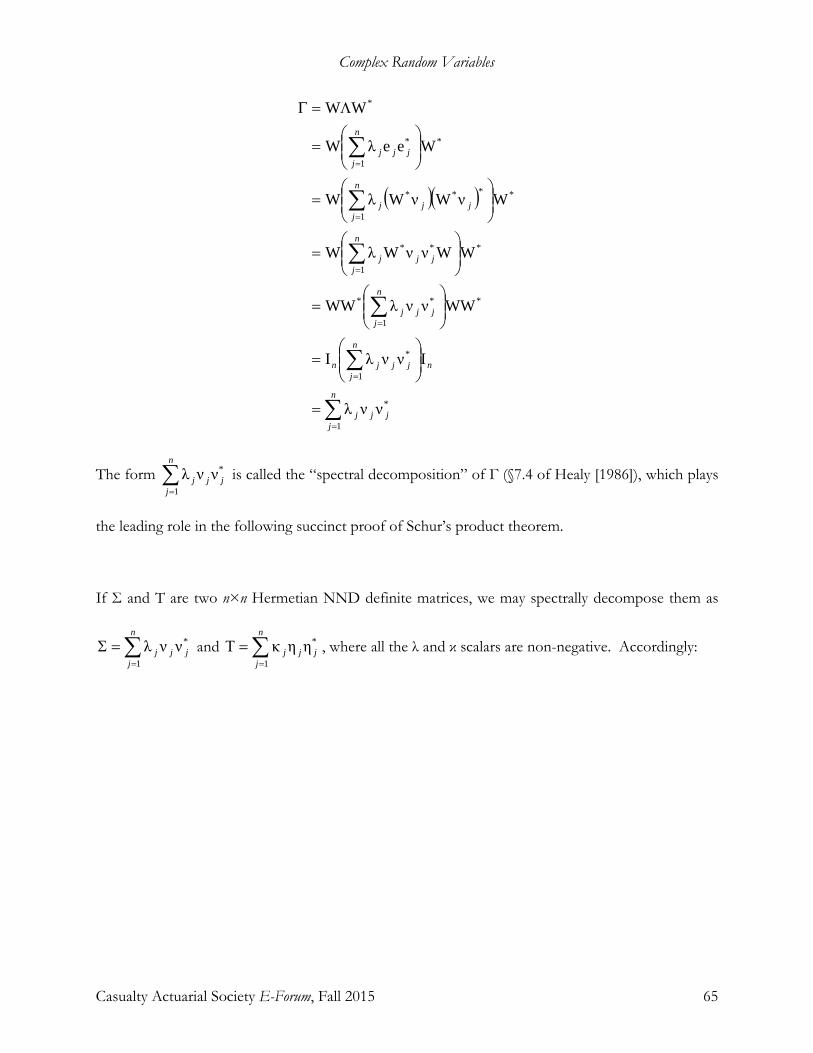
Complex Random Variables
Casualty Actuarial Society E-Forum, Fall 2015 65
( )( )
∑
∑
∑
∑
∑
∑
=
=
=
=
=
=
=
=
=
=
=
=
Λ=Γ
n
jjjj
n
n
jjjjn
n
jjjj
n
jjjj
n
jjjj
n
j
*jjj
1
*
1
*
*
1
**
*
1
**
*
1
***
*
1
*
ννλ
IννλI
WWννλWW
WWννWλW
WνWνWλW
WeeλW
WW
The form ∑=
n
jjjj
1
*ννλ is called the “spectral decomposition” of Γ (§7.4 of Healy [1986]), which plays
the leading role in the following succinct proof of Schur’s product theorem.
If Σ and Τ are two n×n Hermetian NND definite matrices, we may spectrally decompose them as
∑=
=Σn
jjjj
1
*ννλ and ∑=
=Τn
jjjj
1
*ηηκ , where all the λ and κ scalars are non-negative. Accordingly:
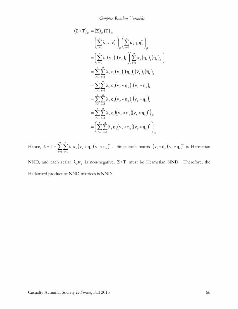
Complex Random Variables
Casualty Actuarial Society E-Forum, Fall 2015 66
( ) ( ) ( )
( ) ( ) ( ) ( )
( ) ( ) ( ) ( )
( ) ( )
( ) ( )
( )( )( )
( )( )jk
n
r
n
ssrsrsr
n
r
n
sjksrsrsr
n
r
n
sksrjsrsr
n
r
n
sksrjsrsr
n
r
n
skskrjsjrsr
n
sksjss
n
rkrjrr
jk
n
ssss
jk
n
rrrr
jkjkjk
=
=
=
=
=
=
=
ΤΣ=ΤΣ
∑∑
∑∑
∑∑
∑∑
∑∑
∑∑
∑∑
= =
= =
= =
= =
= =
==
==
1 1
*
1 1
*
1 1
1 1
1 1
11
1
*
1
*
ηνηνκλ
ηνηνκλ
ηνηνκλ
ηνηνκλ
ηνηνκλ
ηηκννλ
ηηκννλ
Hence, ( )( )∑∑= =
=ΤΣn
r
n
ssrsrsr
1 1
*ηνηνκλ . Since each matrix ( )( )*ηνην srsr is Hermetian
NND, and each scalar srκλ is non-negative, ΤΣ must be Hermetian NND. Therefore, the
Hadamard product of NND matrices is NND.