Embed Size (px)
Citation preview

NBER WORKING PAPER SERIES
NAFTA’s AND CUSFTA’s IMPACTON INTERNATIONAL TRADE
John Romalis
Working Paper 11059http://www.nber.org/papers/w11059
NATIONAL BUREAU OF ECONOMIC RESEARCH1050 Massachusetts Avenue
Cambridge, MA 02138January 2005
I would particularly like to thank my advisors, Daron Acemoglu, Rudi Dornbusch and Jaume Ventura.Thanks for generous support are due to the IMF and Reserve Bank of Australia. Thanks are also due to MarkAguiar, Mary Amiti, Sven Arndt, Christian Broda, Robert Feenstra, Gita Gopinath, Roberto Rigobon, Shang-JinWei, Alwyn Young and participants at seminars and lunches at Chicago GSB, Dartmouth, EIITConference, Federal Reserve Bank of New York, Harvard, IMF, MIT, NAEFA Conference, Penn State,University of Illinois (Urbana), University of Michigan, University of Pennsylvania and USITC. Any errorsare my own. The views expressed herein are those of the author(s) and do not necessarily reflect the viewsof the National Bureau of Economic Research.
© 2005 by John Romalis. All rights reserved. Short sections of text, not to exceed two paragraphs, may bequoted without explicit permission provided that full credit, including © notice, is given to the source.

NAFTA’s and CUSFTA’s Impact on International TradeJohn RomalisNBER Working Paper No. 11059January 2005JEL No. F1
ABSTRACT
This paper identifies the effects of preferential trade agreements on trade volumes and prices using
detailed trade and tariff data. It identifies demand elasticities by developing a difference in
differences based method that exploits the fact that the additional wedge driven between
consumption patterns in a liberalizing versus a non-liberalizing country is directly related to the tariff
reduction. Supply elasticities are identified by using tariffs as instruments for observed quantities.
Analysis of world-wide trade data for 5,000 commodities shows that NAFTA and CUSFTA have
had a substantial impact on international trade volumes, but a modest effect on prices and welfare.
NAFTA and CUSFTA increased North American output and prices in many highly-protected sectors
by driving out imports from non-member countries.
John RomalisThe University of Chicago Graduate School of Business 5807 South Woodlawn Avenue Chicago, IL 60637 and NBER [email protected]

1 Introduction
The growing trend towards preferential trade liberalization depicted in Figure 1 and
the potentially harmful effects of preferential trade agreements on international trade
makes analysis of these agreements important. There are over 200 preferential trade
agreements currently in force, and while almost every country is a party to at least
one such agreement perhaps a more important fact is that typically 200 countries are
not parties to each agreement. This paper seeks to empirically analyze the effects of
the second-largest of these agreements, the North American Free Trade Agreement
(NAFTA), on trade volumes, prices and welfare of both member countries and non-
members. It uses detailed trade data to identify key supply and demand parameters
in a simple static model that is then used to analyze NAFTA. The paper finds that
both supply and demand are very sensitive to price changes. NAFTA therefore has
substantial effects on trade volumes, but price and welfare effects are found to be
modest.
On January 1, 1994 the North American Free Trade Agreement (NAFTA) between
the United States, Canada and Mexico entered into force and incorporated the prior
Canada-US Free Trade Agreement (CUSFTA). For convenience I will often refer to
both agreements simply as “NAFTA”. NAFTA is by far the largest free trade pact
outside of the European Union and is the first reciprocal free trade pact between
a substantial developing country and developed economies (Hufbauer and Schott,
1993). While NAFTA is not a “deep” integration like the European Union, it contains
provisions that go beyond mere removal of tariffs and quantitative trade restrictions,
including disciplines on the regulation of investment, transportation and financial
services, intellectual property, government purchasing, competition policy, and the
temporary entry of business persons (Hufbauer and Schott, 1993). Since the advent
of NAFTA one of the more striking occurrences has been the rapid increase in Mexican
trade. Mexico has become the US’s second largest trading partner, accounting for
11.5 percent of US merchandise imports in 2001 and 13.9 percent of US exports, up
from 6.9 and 9.0 percent respectively in 1993. Only Canada is a partner for more
US trade. Mexico now accounts for a larger share of US trade than Korea, Thailand,
Singapore, Malaysia, Hong Kong and Taiwan combined.
Despite NAFTA’s size, empirical studies often have great difficulty in identifying
2

an effect of NAFTA. The reason for the mixed results in studies of relatively ag-
gregated trade data is very simple. These studies have great difficulty distinguishing
NAFTA’s impact from the impact of two other events that occurred at a similar time.
The first of these events is Mexico’s unilateral trade liberalization that began in 1986.
In general equilibrium, import liberalization also promotes exports. Mexico’s imports
and exports therefore began growing prior to NAFTA. This effect is evident in Figure
2. The second event is the Peso devaluation of 1994-95 that also coincided with rapid
growth in Mexico’s exports.
By contrast, this paper finds that NAFTA has had a substantial impact on trade,
though only a modest effect on prices and welfare. It does so by identifying key supply
and demand elasticities in detailed trade data, and then using those parameters to
estimate the impact of NAFTA on trade volumes and prices. It develops a difference
in differences based estimation technique to identify demand elasticities that focuses
on where each of the NAFTA partners sources its imports of almost 5,000 6-digit Har-
monized System (HS-6) commodities and comparing this to the source of European
Union (EU) imports of the same commodities. The technique enables identification
of NAFTA’s effects on trade volumes even when countries’ production costs shift. In-
verse supply elasticities are identified by regressing observed import prices (excluding
duties) on observed quantities, using tariffs as instruments for observed quantities.
The main advantage of using the detailed trade and tariff data is that it enables
identification of key supply and demand parameters. Studies of aggregate trade pat-
terns are at the mercy of other factors that affect trade. The potential disadvantage is
that product-level studies pay no respect to some general equilibrium considerations
such as trade balance conditions, but this need not be the case.
NAFTA’s impact on trade at the product level can be simply demonstrated with
a few figures. Figure 3A shows that Mexico’s share of US imports has increased most
rapidly in commodities for which it has been given the greatest increase in tariff pref-
erence, defined as the difference between the US tariff on a commodity sourced from
Mexico and the US’s Most Favored Nation (MFN) tariff rate for the same commod-
ity.1 For the 389 commodities where the US tariff preference for Mexican goods has
1The MFN tariff is the tariff applicable to imports from countries that have normal trade relations
with the US.
3

increased by at least 10 percentage points, the simple average of Mexico’s share of US
imports has risen by 224 percent since 1993. For the 2663 commodities where Mexico’s
tariff preference has not increased, its share has risen by a more modest 23 percent.
The timing and cross-commodity pattern of Mexico’s trade increase are themselves
highly suggestive that trade was very responsive to NAFTA’s tariff preferences, and
Figure 3B further supports the case. Figure 3B shows Mexico’s share of EU imports
from 1989-2000. Without the benefit of a free trade agreement until late 2000, the
evolution of Mexico’s trade with the EU has been very different. Its share of EU
imports of commodities with high NAFTA preferences declined by 77 percent, while
its share of EU imports of commodities where NAFTA did not increase preferences
rises by 64 percent. This growing wedge between US and EU import patterns will
identify demand elasticities and, when combined with estimated supply elasticities,
NAFTA’s impact on trade volumes and prices.
Canada’s share of US imports has also increased since CUSFTA came into effect
in 1989, and Figures 4A to 4C also suggest that CUSFTA was partly responsible. For
commodities where there was no increased preference for goods of Canadian origin,
Canadian goods now account for a 2 percent smaller share of US imports than they did
in 1988. But where the preference increased by at least 10 percentage points, Canada’s
share of US imports increased by 99 percent. The timing and cross-commodity pat-
tern again suggest that CUSFTA is at work. Figure 4C shows Canada’s share of
US imports from 1980 to 2000. For most of the 1980s, Canada’s share of US im-
ports is declining in all tariff classes, but just before CUSFTA, Canada’s share begins
to rebound for commodities where large tariff preferences were negotiated. Figure
4B provides a comparison with Canada’s trade with the EU, which does not have a
preferential trade agreement with Canada. For the commodities with no CUSFTA
preferences, Canada’s share of EU imports has declined by 6 percent. For commodi-
ties with high CUSFTA preferences, Canada’s share of EU imports has declined by 40
percent. Figures 3A to 4C together suggest that NAFTA/CUSFTA have had a sub-
stantial impact on trade, and even though US tariffs are typically low, trade appears
to be quite sensitive to even small trade preferences.
Preferential Trade Areas (PTAs) have received a great deal of analytical and em-
pirical attention since Viner (1950) distinguished between the trade creation and trade
diversion effects of preferential tariff liberalization. Much of this attention is driven
4

by the ambiguous welfare implications of PTAs. Favorable effects (“trade creation”)
result from removing distortions in the relative price between domestically produced
commodities and commodities produced in other members of the PTA. Unfavorable
effects (“trade diversion”) come from the introduction of distortions between the rel-
ative price of commodities produced by PTA members and non-members (Frankel,
Stein and Wei 1996). Research has also been motivated by the political economy of
PTAs, such as whether PTAs help or hinder movement towards the first best of global
free trade (for example, Baldwin 1996, Levy 1997, Bagwell and Staiger 1999).
Much empirical work has been devoted towards evaluating trade and welfare ef-
fects of PTAs (Baldwin and Venables 1995). One major group of studies of PTA’s are
ex-ante simulations using Applied General Equilibrium (AGE) models that produce
price and welfare predictions in addition to trade volume predictions. The other ma-
jor group are ex-post studies examining changes in the direction of aggregate trade
between countries or regions following the introduction of the PTA. Examples of
AGE modelling of NAFTA are Kehoe and Kehoe (1995), Brown, Deardorff and Stern
(1995), Cox (1995), Sobarzo (1995) and studies surveyed in Baldwin and Venables
(1995). All models predicted welfare gains for NAFTA members, though the wel-
fare estimates are sensitive to whether the models are “first generation” with perfect
competition and no dynamics, “second generation” with increasing returns and im-
perfect competition, or “third generation” with the addition of capital accumulation.
Later generation models have more potential for welfare changes and typically sug-
gest greater welfare gains. Examples of ex-post studies that use aggregate trade data
for NAFTA are Gould (1998) and Garces-Diaz (2001). Gould finds that NAFTA has
increased US-Mexico trade, but has had no effect on US-Canada or Mexico-Canada
trade. Garces-Diaz finds that Mexico’s export boom is not attributable to NAFTA.
Papers more similar to this are Clausing (2001), Fukao, Okubo and Stern (2003),
Krueger (1999, 2000) and Chang and Winters (2002). Clausing was first to exploit
tariff variation at the detailed commodity level using US import data from 1989 to
1994. Clausing finds that US import growth was related to tariff preferences conferred
on Canada and also concludes that CUSFTA was primarily trade creating. Fukao,
Okubo and Stern analyze US imports at the HS 2-digit level for the period 1992-
1998. Of the 70 sets of industry regressions they run, NAFTA tariff preferences had a
significant effect on US imports in 15 cases. Research at the 3 and 4-digit SIC industry
5

level by Krueger (1999, 2000) finds no evidence that NAFTA has had any impact on
intra-North American trade. In a study of MERCOSUR, Chang and Winters (2002)
examine export price data for five non-member countries. They find that due to
the tariff preference, competition from Argentina, Uruguay and Paraguay has led to
significant and substantial reductions in American, Chilean, German, Korean and
Japanese export prices to Brazil.
Related papers include Kehoe and Ruhl (2002), who find that growth in the
extensive margin following trade liberalizations is an important source of new trade,
especially for the previously thin Canada-Mexico trade relationship. Head and Ries
(1999) study the industry rationalization effects of tariff reductions and find that on
balance, NAFTA has had little net effect on the scale of Canadian firms. Trefler
(2001) finds that Canadian industries that experienced the largest tariff cuts under
NAFTA experienced substantial labor productivity gains, but a decline in both output
and employment. Yeats (1997) finds that the fastest growth in intra-MERCOSUR
trade was in commodities in which members did not display a comparative advantage,
inferred from the lack of exports of these commodities outside MERCOSUR. This was
interpreted as evidence of the trade diversion effects of MERCOSUR.
This paper is organized as follows. Section 2 introduces a simple “first genera-
tion” model of preferential trade liberalization that is used to derive the estimating
equations and underpin the welfare analysis. Section 3 describes the data. Section 4
presents and discusses the empirical results. Section 5 concludes.
2 Theoretical Framework and Empirical Strategy
This paper seeks to exploit the commodity and time variation in the tariff prefer-
ence that is afforded to goods originating in NAFTA partners to identify NAFTA’s
and CUSFTA’s effect on trade and welfare. The paper identifies demand elasticities
by focusing on where NAFTA members and the EU source their imports of different
commodities. It seeks to explain changes in North American import sources using the
preference afforded to commodities of North American origin. The idea is that where
North American output is afforded no new preference (where the MFN tariff rate is
zero, for instance), NAFTA’s only impact should come through a general equilibrium
6

effect on output prices, or through reductions in “border effects” due to NAFTA pro-
visions that go beyond tariff liberalization. For commodities where NAFTA causes a
new preference to open up for North American goods, the preference should have an
additional effect causing North American consumers to substitute towards newly pre-
ferred goods and away from other sources of supply. Supply elasticities are identified
using tariffs as instruments that, for a given supply price, shift the demand curve.
This strategy can be derived from a simple model. The model and the estimated
parameters are then used to evaluate NAFTA’s effects on trade volumes, prices and
welfare.
A. Model Description
Firms produce commodities under perfectly competitive conditions. Trade is
driven by preference for variety and by commodities being differentiated by coun-
try of origin. Countries may impose ad-valorem tariffs on imports. Countries may
then enter into preferential trading agreements whereby each country in the agree-
ment lowers tariffs on imports from partner countries but need not adjust the tariff on
imports from other countries. This causes consumers to substitute towards the output
of preferred countries and away from all other sources of supply, including domestic
production. Factor supplies are not explicitly modelled. The model assumptions are
set out in detail below.
1. Countries are denoted by c and time by t.2
2. There is a continuum of industries z on the interval [0,1]. In each country, every
industry produces a commodity using an industry-specific factor under conditions
of perfect competition with marginal cost at¡qSt (zc)
¢(henceforth often denoted as
at (zc)), where qSt (zc) is production of commodity z in country c. Note that marginal
cost depends on the quantity produced and may vary across producing country and
time. I assume a constant inverse supply elasticity:
ln at¡qSt (zc)
¢= η (zc) ln q
St (zc) + ln
bPct +Dct +Dcz + εczt (1)
2In the empirical analysis “country” will often mean collection of countries such as the European
Union or a “Rest of the World” group of countries. Aggregation is discussed in the Appendix.
7

where η (zc) is the inverse supply elasticity, bPct is the aggregate price index in
country c, Dct is a country-by-year fixed effect, Dcz is a country-by-product fixed
effect and εczt is a random supply shock.
3. In every period consumers in each country are assumed to maximize Cobb-
Douglas preferences over their consumption of the output of each industry, Qct (z),
with the fraction of income spent on industry z being bc (z) (Equations 2 and 3).
Expenditure shares for each industry are therefore constant for all prices and incomes.
Uct =
1Z0
bc (z) lnQct (z) dz. (2)
1Z0
bc (z) dz = 1. (3)
4. The output of each industry is not a homogeneous good. Although firms in
the same country produce identical goods, production is differentiated by country
of origin. Qct (z) can be interpreted as a sub-utility function that depends on the
quantity of each variety of z consumed. I choose the CES function with elasticity
of substitution σz > 1. Let qDct (zc0) denote the quantity consumed in country c of
commodity z produced in country c0. Qct (z) is defined by Equation 4:
Qct (z) =
ÃNX
c0=1
qDct (zc0)σZ−1σZ
! σZσZ−1
. (4)
5. There may be transport costs for international trade. Transport costs are intro-
duced in the convenient ‘iceberg’ from; gc0t (zc) units must be shipped from country
c for 1 unit to arrive in country c0; gct (zc) = 1, ∀c.
6. Tariffs: τ c0t (zc)− 1 is the ad-valorem tariff imposed by country c0 on imports
of commodity z from country c; τ ct (zc) = 1, ∀c. Tariffs are rebated as a lump-sum toconsumers.
8

B. Equilibrium
In equilibrium, consumers maximize utility, firms maximize profits and trade is
balanced. Because of the assumption of perfect competition, prices (exclusive of tariffs
and transport costs) are equal to marginal cost, at (zc) . Consider the consumers in
country 1, which will be a NAFTA country and for now we will call the US. Tariffs
and transport costs raise the price paid by US consumers for goods imported from
country c to at (zc) g1t (zc) τ1t (zc). Let T1t (z) denote tariff revenue collected in the
US on imports of commodity z, let Y1t denote US income, and qD1t (zc) denote US
consumption of commodity z produced in country c. US income is equal to the sum
of firm revenues plus tariff revenue.3
T1t (z) =Xc
(τ 1t (zc)− 1) qD1t (zc) at (zc) , (5)
Y1t =
1Z0
at (z1) qSt (z1) dz +
1Z0
T1t (z) dz. (6)
US consumers maximize utility subject to expenditure being equal to income in
every period:
Xc
qD1t (zc) at (zc) g1t (zc) τ 1t (zc) = b1 (z)Y1t. (7)
Differentiating the Lagrangian for the consumers’ constrained optimization prob-
lem with respect to consumption levels of each commodity, we find that the tariff on
imported goods causes domestic consumers to substitute towards domestically pro-
duced varieties. The amount of substitution depends on the level of the tariff and on
the elasticity of substitution between varieties:
∀z,∀c, ∀t, qD1t (zc)
qD1t (zc0)=
µτ 1t (zc0)
τ1t (zc)
¶σZ µat (zc0)at (zc)
¶σZ µg1 (zc0)g1 (zc)
¶σZ
. (8)
3Revenue from firm sales will all accrue to factors of production (inputs), which are assumed to
be domestically owned. Underlying factor markets are not modelled.
9

Equilibrium conditions for all other countries are symmetric, which will be ex-
ploited by the empirical work to control for the effect of unobserved movements in
marginal cost that may be correlated with tariff movements. Finally, all commodity
markets have to clear, taking into account output that melts in transit:
∀z, ∀c,∀t, qSt (zc) =Xc0qDc0t (zc) gc0t (zc) . (9)
C. Empirical Strategy
(i) Demand Elasticity
I use Equation 8 to derive estimating equations for demand elasticities. Equivalent
equations exist for every other country, specifically, let country 2 be the aggregate
of the twelve countries that were always members of the EU for the sample period
1989-1999:
∀z, ∀c,∀t, qD2t (zc)
qD2t (zc0)=
µτ2t (zc0)
τ2t (zc)
¶σZµat (zc0)
at (zc)
¶σZµg2t (zc0)
g2t (zc)
¶σZ
. (10)
Using Equations 8 and 10 we can eliminate the marginal cost terms:
lnqD1t (zc)
qD1t (zc0)− ln qD2t (zc)
qD2t (zc0)= σz
·ln
τ1t (zc0)
τ1t (zc)− ln τ 2t (zc0)
τ2t (zc)
¸+σz
·ln
g1t (zc0)
g1t (zc)− ln g2t (zc0)
g2t (zc)
¸. (11)
Elimination of the unobserved marginal cost terms is important because relative
costs will shift following a trade liberalization. Equation 11 can be transformed into
an equation for Cost including Insurance and Freight (CIF) import values, to match
how EU trade data are collected:
10

lnat.g1t.q
D1t (zc)
at.g1t.qD1t (zc0)
− ln at.g2t.qD2t (zc)
at.g2t.qD2t (zc0)
= σz
·ln
τ1t (zc0)
τ1t (zc)− ln τ2t (zc0)
τ2t (zc)
¸+(σz − 1)
·ln
g1t (zc0)
g1t (zc)− ln g2t (zc0)
g2t (zc)
¸. (12)
So long as I only examine countries c and c0 for which the EU does not change
its relative tariffs, ln τ2t(zc0 )τ2t(zc)
is simply a commodity fixed effect. Since I do not have
detailed transport cost data for EU trade, to identify σZ I assume that relative trans-
port costs of shipping commodities to the US and the EU, ln g1t(zc0)g1t(zc)
− ln g2t(zc0)g2t(zc)
, is the
sum of a commodity fixed effect, a year fixed effect and an error term that is orthog-
onal to US tariffs.4 This produces the basic demand elasticity estimating Equation
13 based on CIF import values, where Dz and Dt are full sets of commodity and year
dummies respectively, while εcc0z is a random disturbance term:
lnat.g1t.q
D1t (zc)
at.g1t.qD1t (zc0)− ln at.g2t.q
D2t (zc)
at.g2t.qD2t (zc0)=Dz +Dt + σz ln
τ 1t (zc0)
τ1t (zc)+ εcc0z (13)
Now consider country c to be Canada or Mexico and country c0 to be any other
country. NAFTA’s and CUSFTA’s increase in the US tariff preferences for Canadian
and Mexican goods, ln τ1t(zc0)τ1t(zc)
, will increase the share of those goods in US consump-
tion relative to their share of EU consumption. The size of the increased share in an
arbitrary industry z depends positively on the size of the increased US tariff prefer-
ence, and positively on the elasticity of substitution σ between varieties of z.
The choice of EU as “country 2” to identify demand elasticities is of minor im-
portance to the empirical analysis. The EU was chosen for two main reasons. Firstly,
its detailed trade data has long been available electronically. Secondly, the European
Union is a relatively large trading partner for the US, Canada and Mexico, which
4The assumption may not be completely innocuous. The most significant recent feature of interna-
tional trade costs has been the relative decline in air-freight costs. This is likely to disproportionately
benefit some commodities and some trade routes. See Hummels (1999) for a detailed examination
of international trade costs.
11

maximizes the number of products that can be used to estimate demand elasticities
and increases the precision of the estimates. The cost of choosing the EU as country
2 is that the EU is excluded from the list of control countries c0. This means that the
paper does not directly use some of the substitution between the output of NAFTA
countries and EU output to identify demand elasticities. For transparency purposes
I also report estimates obtained using all trade involving NAFTA countries or EU
countries, including trade between EU members, but note that relative EU tariffs
ln τ2t(zc0 )τ2t(zc)
are no longer a commodity fixed effect.
(ii) Supply Elasticity
In Equation 1 the marginal cost of producing a commodity in country c was
allowed to increase with the quantity produced in that country. NAFTA countries
may face an elasticity of supply that is less than infinite, so that demand shifts caused
by preferential trade liberalization affect equilibrium prices. These price changes
are an important ingredient of welfare analysis and it is necessary to estimate how
prices respond to preferential trade liberalization. The mean supply elasticity can be
estimated in a manner that mostly utilizes very detailed price and quantity data for
US imports. Taking Equation 1 and noting that qSt (zc) =P
j qSjt (zc):
ln at (zc) = η (zc)
"− ln qS1t (zc)P
j qSjt (zc)
+ ln qS1t (zc)
#+ bPct +Dct +Dcz + εczt (14)
where qS1t(zc)Pj q
Sjt(zc)
is the share of Country c’s output of zc that is exported to the
US, η (zc) is the inverse supply elasticity, Dct and Dcz are full sets of country-by-year
dummies and country-by-product dummies, and εczt are random supply shocks. The
aggregate price index bPct is absorbed by the fixed effects Dct. Tariff-line level data
(15,000 commodities) exists for supply prices at (zc) and quantities qS1t (zc) supplied to
the US. I estimate the share of Country c’s output of zc that is exported to the US at
the HS 6-digit level (5000 commodities). The World Bank’s WITS database contains
bilateral trade data for most countries at the HS 6-digit level for some years between
1989-1999 (depending on reporting country). For each available reporting country
and year, I extract the share of their exports of each HS 6-digit product that are
12

exported to the US. I then multiply this by the fraction of each reporting country’s
GDP that is exported to estimate the required share. The parameter η (zc) can be
identified using tariffs as an instrument since, for a given supply price at (zc), tariffs
shift demand. This can be seen from the demand equation. From the model’s CES
demand assumption, demand for product zc is given by:
ln qD1t (zc) = −σz ln at (zc)− σz ln τ1t (zc)− σz ln g1t (zc) + (σz − 1) ln bP1tz + ln b1 (z)Y1t(15)
where bP1tz is the ideal price index for commodity z in the US:bP1tz = "X
c
(at.g1t.τ 1t (zc))1−σ# 11−σ
(16)
Any change in tariffs imposed by the US on imports of product z from any source
will shift the demand curve for zc, because the tariff changes shift either τ 1t (zc), the
price index bP1tz or both. These movements in the demand curve identify the supplycurve.
3 Data Description
(i) International trade data
International trade data for almost all of the world is now collected according
to the Harmonized System (HS), a schedule that is standard across countries at the
6-digit level, or approximately 5,000 commodities. Most of this data is available
from the World Bank’s WITS database. For some key countries I use more complete
national sources of data. The US International Trade Commission (USITC) maintains
a database at the 10-digit level (15,000 commodities) of US imports classified by
commodity, country of origin, import program, month and port of arrival. Eurostat
and Statistics Canada maintain similar databases for the EU and Canada.
13

For the purposes of Figures 2 to 4C it is useful to keep a balanced panel of
products. Changes in HS commodity classifications lead to some attrition, but I am
able to track US and EU trade in 4,655 6-digit commodities annually from 1989 to
2000. Because Canada entered into CUSFTA with the US in 1989, it is useful to
collect data for earlier years. Prior to 1989, US trade data was collected according
to a different commodity schedule, the TSUSA. Concordances are available for this
data, but revisions to the TSUSA also lead to attrition. I am able to track 4,483
commodities continuously from 1988 to 2000, and 3,592 from 1980 to 2000.
The data also contains information on physical quantities imported for most com-
modities, allowing the calculation of unit price variables. I estimate supply elasticities
using these prices.
(ii) Tariff Data
Tariff data is also collected from both national sources and theWorld Bank’sWITS
database. Tariff data is based on either tariff schedules or detailed data on import
duties collected. US tariff schedules for the years 1997 to the current year are available
from the USITC. I extracted US tariff data for 1989 to 1996 from USITC files.5 US
tariffs are almost invariably set at the HS 8-digit level (10,000 commodities). While
most tariffs are ad-valorem, there are still several hundred specific tariffs applied. The
USITC calculates the ad-valorem equivalent of any specific tariffs. The distribution of
US MFN tariffs in 1999 is illustrated in Figure 5A. The simple average of tariff rates
is low at 5.2 percent, but importantly there is a large amount of dispersion, with the
standard deviation of MFN tariff rates being 12 percent. Under NAFTA, all but a
couple hundred of these tariffs have been eliminated for Canada and are in the process
of being eliminated for Mexico, creating a large variation in the preference given to
goods of Canadian or Mexican origin (Figure 5B). Table 1 shows that much of this
variation occurs within fine product classifications. Table 1 reports the percentage of
the variance of US MFN tariff rates and tariff preferences for Canada and Mexico at
the tariff-line level that can be explained by full sets of dummy variables for broader
industry classifications. Much of the tariff variation remains unexplained by these
variables, therefore existing industry-level studies of NAFTA ignore most of the tariff
variation.5This data was made available by Feenstra, Romalis and Schott (2002).
14

Preferential treatment for some goods existed prior to CUSFTA/NAFTA. In 1965,
Canada and the US negotiated the Auto-Pact, allowing duty-free trade in many
automotive goods. The Auto Pact was incorporated into CUSFTA. Mexico was a
beneficiary of the Generalized System of Preferences (GSP), under which the US
(and other developed countries) gave developing countries preferential access to their
markets. The US gave duty free access to the output of developing countries for
several thousand HS 8-digit commodities, although goods where developing countries
may have gained most from preferential access were often excluded (notably many
agricultural items and textiles, clothing and footwear), and the preference could be
removed under “competitive needs limitations” to the GSP. Details of the Auto Pact
and GSP program are included in the tariff schedules. Although the US engaged in
some fine tuning of the GSP program, there are only two changes that affected a
significant amount of US trade during the sample period. The first was the expulsion
(“graduation”) of Hong Kong, Korea, Singapore and Taiwan from the scheme at the
end of 1988. This can be accommodated by dropping either pre-1989 data or these
four countries from the analysis - I drop the pre-1989 data.6 The second change was
that upon entry into NAFTA, Mexico was no longer entitled to claim GSP benefits
for trade with the US.
Tariffs are aggregated from the HS 8-digit level to the 6-digit level in two different
ways: by taking simple averages; or by taking trade weighted averages. There are
several limitations to using tariff schedules to calculate tariffs. One limitation is the
effect of the maquiladoras on Mexican exports to the US. Under ‘production sharing’
provisions US duty does not have to be paid on the US sourced content of many
exports to the US, while the full value of those transactions is recorded in US trade
data. Mexico will also not collect duty on many intermediate inputs that are destined
to be exported. Tariff schedules will therefore often overstate the NAFTA preferences.
A second limitation of the tariff schedule is that preferential tariff arrangements are
often circumscribed by restrictive rules of origin that need to be satisfied to qualify
for the tariff preference. To partly address these limitations I also calculate tariffs
using data on actual import duty paid. The drawback of this approach is that tariff6There is a detailed concordance between the 1988 and 1989 US data detailing the change in
trade and tariff schedules. I considered that keeping a broader set of comparison countries was more
important than keeping an extra year of data. The substitution elasticity estimates are not very
sensitive to this choice.
15

rates can only be observed when there is trade. Where there is no trade, I revert to
the tariff schedule for that item. This alternative set of 8-digit “applied” tariffs are
also aggregated to the 6-digit level using simple averages and trade weighted averages.
This gives a total of four measures of tariffs at the HS 6-digit level.
Quantitative restrictions on imports of many textile, clothing and footwear com-
modities under the Multi-Fibre Agreement (MFA) and of many agricultural commodi-
ties provide a further complication. Many of these restrictions are binding, although a
large number are not (Carolyn Evans and James Harrigan, 2003). They are extremely
difficult to account for, since many restrictions encompass many HS commodities and
most apply bilaterally. The existence of binding quotas will tend to bias downwards
the estimated substitution elasticities. Eliminating commodities subject to quotas
did not, however, lead to higher substitution elasticity estimates.
The preferences given to Canadian and Mexican production are systematically
related to some of the characteristics of the commodities. This is evident from Figures
3A to 4C showing a systematic negative relationship between the preference and
Canada’s and, to a lesser extent, Mexico’s share of US imports. Canadian and, to a
lesser extent, Mexican tariffs are strongly correlated with US tariffs.7 Given that the
most protected sectors are agriculture and simple manufactures like textiles, apparel
and footwear, the highest preferences are mostly in these sectors, subject to the
existence of quantitative restrictions. The NAFTA preferences are biased towards
commodities in which developed countries have a comparative disadvantage. This
effect can also be seen in price data in Tables 2A to 2C. The relative price of Canadian
and US goods is usually substantially higher in commodities where there are large
tariff preferences under NAFTA. This suggests that NAFTA may have caused an
expansion of North American production of commodities for which North America is
a relatively high cost producer.
Data on Canadian import duties charged is collected for all years and products by
Statistics Canada. The ad-valorem component of tariff schedules is also available for
most years for many countries, including Canada and Mexico, from the World Bank’s
WITS database. Canadian tariff data is aggregated to the 6-digit level in the same
7The simple correlations of HS 6-digit tariffs is 0.5 for the US and Canada, 0.25 between the US
and Mexico, and 0.35 between Canada and Mexico.
16
way as US tariff data. Mexican trade data is only available at the 6-digit level in
the WITS database, so Mexican tariffs were aggregated to the 6-digit level by taking
simple averages. I can therefore estimate demand elasticities using the imports of
each of the NAFTA partners.
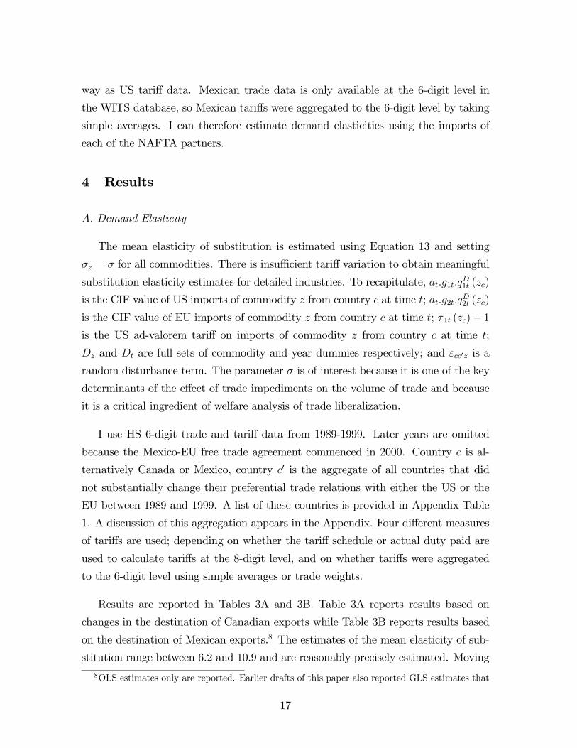
4 Results
A. Demand Elasticity
The mean elasticity of substitution is estimated using Equation 13 and setting
σz = σ for all commodities. There is insufficient tariff variation to obtain meaningful
substitution elasticity estimates for detailed industries. To recapitulate, at.g1t.qD1t (zc)
is the CIF value of US imports of commodity z from country c at time t; at.g2t.qD2t (zc)
is the CIF value of EU imports of commodity z from country c at time t; τ 1t (zc)− 1is the US ad-valorem tariff on imports of commodity z from country c at time t;
Dz and Dt are full sets of commodity and year dummies respectively; and εcc0z is a
random disturbance term. The parameter σ is of interest because it is one of the key
determinants of the effect of trade impediments on the volume of trade and because
it is a critical ingredient of welfare analysis of trade liberalization.
I use HS 6-digit trade and tariff data from 1989-1999. Later years are omitted
because the Mexico-EU free trade agreement commenced in 2000. Country c is al-
ternatively Canada or Mexico, country c0 is the aggregate of all countries that did
not substantially change their preferential trade relations with either the US or the
EU between 1989 and 1999. A list of these countries is provided in Appendix Table
1. A discussion of this aggregation appears in the Appendix. Four different measures
of tariffs are used; depending on whether the tariff schedule or actual duty paid are
used to calculate tariffs at the 8-digit level, and on whether tariffs were aggregated
to the 6-digit level using simple averages or trade weights.
Results are reported in Tables 3A and 3B. Table 3A reports results based on
changes in the destination of Canadian exports while Table 3B reports results based
on the destination of Mexican exports.8 The estimates of the mean elasticity of sub-
stitution range between 6.2 and 10.9 and are reasonably precisely estimated. Moving
8OLS estimates only are reported. Earlier drafts of this paper also reported GLS estimates that
17

across the columns, the estimates are slightly sensitive to the choice of tariffmeasure -
the estimates using Canadian exports are lower when the tariff schedule is used. The
estimates based on Mexican exports tend to be higher than those based on Canadian
exports. The estimates are very similar whether the ‘control’ countries c0 are limited
to those listed in Appendix Table A1 or include all non-NAFTA countries. The esti-
mates are similar in magnitude to elasticities estimated by Clausing (2001) and Head
and Ries (2001).
These elasticities of substitution suggest that consumers are very willing to substi-
tute between different sources of a commodity. One implication of this willingness to
substitute is that small costs to international trade, whether due to natural barriers
such as transport costs or artificial barriers such as tariffs, will have a large effect on
trade volumes. With a substitution elasticity of 6, ignoring for a moment terms of
trade effects, the median US tariff of 5.5 per cent will reduce consumption of imported
varieties relative to domestic varieties by 27 per cent. With a substitution elasticity
of 11, this reduction in relative consumption is 45 per cent. But on some products
the effect of trade barriers will be much more dramatic; US tariffs range up to 350
per cent.
I also estimate Equation 13 using, alternately, Canada and Mexico as “Country 1”.
The trade and tariff data were obtained at the HS 6-digit level for Mexico and Canada
from the World Bank’s World Integrated Trade Solution (WITS) database, and at the
tariff-line level for Canada from Statistics Canada. One caveat with these results is
that the tariff schedules in theWITS database only include the ad-valorem component
of tariffs, and are not available for all years.9 This is not a severe limitation in the case
of Canada, because Canadian data on duties collected are available for all years at
the tariff-line level and these “applied” tariffs can also be used to estimate elasticities.
Substitution elasticity estimates obtained using Canada’s applied tariffs and reported
in Tables 3C and 3D ranged from 5.0 to 5.5 when examining the destination of US
exports and 7.2 to 8.1 when examining Mexican exports. The estimates obtained
using Mexican tariff data and reported in Table 3E are much lower, at 2.0 to 2.5
sought to exploit the serial correlation of the disturbances and Heckman estimates that sought to
model the missing observations. These estimates were very similar.9Canadian tariff schedules for 1990-1992 and 1994 had to be estimated from surrounding years’
data, as did Mexican tariff schedules for 1990, 1992-1994 and 1996.
18

when examining US exports and 0.6 to 0.8 when examining Canadian exports. These
low estimates partly result from the greater measurement error in the Mexican tariff
data, but may also result from a important force driving Mexican imports being the
US tariff reductions on Mexican goods containing sufficient North American content,
stimulating Mexican imports of components from the US and Canada.
B. Supply Elasticity
I estimate the mean inverse supply elasticity using Equation 14 and setting η (zc) =
η for all products. I obtain both IV and OLS estimates using the most detailed US
import price and quantity data available, the 10-digit level. Estimation of Equation 14
requires estimates of the share of Country c’s output of zc that is exported to the US.
The World Bank’s WITS database contains bilateral trade data for most countries
at the HS 6-digit level for some years between 1989-1999 (depending on reporting
country). For each available reporting country and year, I extract the share of their
exports of each HS 6-digit product that are exported to the US. I then multiply this
by the fraction of each reporting country’s GDP that is exported to estimate the
required share.
I use four tariff rates as instruments for the observed output quantity in Equation
14. Firstly, I use the US tariff rates on exports from Country c, Canada, Mexico and
all other countries. Secondly, I only use the tariff rate on exports from Country c. An
increase in this tariff will, conditional on the supply price, shift demand downwards.
Thirdly, I omit the tariff rate on exports from Country c but include the other three
tariff measures. An increase in these tariff rates will, conditional on the supply price
and the tariff on exports from Country c, shift demand for zc upwards. Tariffs are
measured at the 10-digit level using data on duties paid. Where data on duties paid
is not available, I use the tariff schedule.10 I omit all products where there is a
specific tariff, because a specific tariff generates a causal link from supply prices to
the measured ad-valorem equivalent tariff.
Column 1 of Table 4 contains results where the four tariff rates are used as an
instrument for quantity. I estimate the parameter η to be 0.29. This result suggests
that supply to the US is fairly elastic, even for products zc where the US consumes
10When the tariff schedule is used the MFN rate is used for the “all other countries” tariffmeasure.
19

most of the output. A shock to demand that causes a 1 percent increase in worldwide
consumption of zc will cause the supply price to increase by 0.29 percent. Column 2
reports the results when the tariff on exports from Country c is the only instrument.
The estimate of η is unchanged at 0.29. Column 3 reports the results when the
tariff on exports from Country c has been omitted from the set of instruments. The
estimate of η is less precisely estimated and slightly lower at 0.22. Column 4 reports
OLS results purely for inspection, they have no useful interpretation since OLS does
not identify the supply curve.
With estimates of demand and supply elasticities at hand we now have the two
essential parameters for welfare analysis of NAFTA.
C. Welfare and Trade Volume
With estimates of demand and supply elasticities it is possible to make tentative
calculations of NAFTA’s and CUSFTA’s price and welfare effects without invoking
the greatly simplifying “small country” assumption. I use the simple model in Section
2 of the paper. The model, while extremely parsimonious with parameters, will be
applied to rich trade and tariff data. This calculation will be incomplete, but it will be
consistent with the structure of the model and the estimated parameters. The strategy
is to estimate the first-order welfare effects of CUSFTA and NAFTA on the USA,
Canada, Mexico and the Rest Of the World (“ROW”). The important ingredients
of that calculation are reported in this section, the details of that calculation and
additional data requirements are left to the Appendix.
I estimate the effects of each trade agreement on the purchasing power of a coun-
try’s output, holding output quantities constant. Nominal income is given by Equa-
tion 6, and the ideal price index corresponding to the utility function in Equation 2
is:
bPct =Yz
"Xc0(at.gct.τ ct (zc0))
1−σ# bc(z)
1−σ
. (17)
This measure will understate welfare because it will fail to account for a second-
order effect from the reoptimization of production and factor supply following changes
20

in relative prices. The calculations proceed in four steps. Firstly, I estimate how prices
and quantities of each product respond to the tariff liberalization, keeping existing
aggregate income constant. I then use product prices and industry price indexes to
estimate expenditures on each country’s goods and the change in aggregate incomes.
These new aggregate incomes are then used to recalculate equilibrium product prices.
This process is iterated until the estimated changes in prices and incomes are consis-
tent with no change in each countries’ trade balance. Welfare calculations are then
performed.
(i) Equilibrium
From Equation 1, ignoring fixed effects and supply shocks, the inverse supply
curve is:
ln at (zc) = η ln
ÃXc0qSc0t (zc)
!+ ln bPct (18)
Totally differentiating Equation 18 yields:
d ln at (zc) = η
ÃXc0sc0t (zc) d ln q
Sc0t (zc)
!+ d ln bPct (19)
where sc0 (zc) =qSc0t(zc)Pj q
Sjt(zc)
is simply the proportion of the output of zc that is
supplied to country c0. Totally differentiating the demand Equation 15 yields:
d ln qDc0t (zc) = −σd ln at (zc)− σd ln τ c0t (zc)− σd ln gc0t (zc)+ (σ− 1)d ln bPc0tz + d lnYc0t
(20)
In equilibrium, the change in demand due to NAFTA will equal the change in
supply. Substituting d ln qDc0t (zc) from Equation 20 for d ln qSc0t (zc) in Equation 19
and ignoring transport costs (that I assume to be unchanged) yields how equilibrium
21

supply prices at (zc) change in response to changed tariffs, industry price indexes bPc0tz
(defined in Equation 16), aggregate price indexes bPct and aggregate incomes:
d ln at (zc)=η
1 + ησ[Xc0− sc0 (zc) σd ln τ c0t (zc) +
Xc0sc0 (zc) (σ − 1)d ln bPc0tz
+Xc0sc0 (zc) d lnYc0t +
1
ηd ln bPct] (21)
Equation 21 together with Equations 16, 17 and 6 defining bPc0tz, bPct and Yc0t form a
non-linear system of equations involving hundreds of thousands of products. I make
one modification to the system to make the general equilibrium not too computa-
tionally burdensome to solve numerically. I group all non-NAFTA countries into the
aggregate ROW. Although I treat the output of each country in the ROW as a sepa-
rate product, I compute the change in the aggregate income for the ROW and price
indexes bPc0tz and bPct that are common to every country in the ROW.
The solution is obtained iteratively in four steps. Firstly, the change in tariffs un-
der CUSFTA/NAFTA is inserted into Equation 21 to yield estimates of price changes
of individual products d ln at (zc). This only captures the ‘proximate’ effect of the tar-
iff reductions on the price of output produced in NAFTA countries. In the second
step these new prices are then used to construct the change in price indexes d ln bPc0tz
and d ln bPct using Equations 16 and 17. The change in these price indexes are then
used in the third step to reestimate the price changes of individual goods using Equa-
tion 21. This time the prices of all goods in an industry are affected if there were
any tariff changes in that industry. Iterating the second and third steps quickly leads
to convergence of the individual goods prices and the price indexes. In the fourth
step these new prices and price indexes are used to estimate the change in income
d lnYc0t. I use the fact that in an equilibrium with an unchanged trade balance, the
change in a country’s income equals the change in expenditures on its output (net of
taxes and transport costs) plus the change in taxes collected on imported goods. The
change in quantities demanded are estimated by substituting the tariff reductions and
the changes in goods prices, price indexes and aggregate incomes into Equation 20.
Changed expenditures and trade taxes are then a simple function of the tariff reduc-
tions and the estimated price and quantity responses. Iterating the second through
22

fourth steps leads to convergence in the estimates of goods prices, price indexes and
national incomes. More details of solving for the change in equilibrium prices are in
the Appendix.
(ii) Welfare and Trade Volume
The welfare decomposition for CUSFTA and NAFTA is summarized in Table 6.
Increases in the real value of output of NAFTA members is offset by the decline in
tariff revenue, leaving small welfare changes in this simple static model. To an extent
the welfare result is not surprising, because the model omits many of the potential
channels of welfare changes such as entry and exit of varieties, firm heterogeneity,
scale economies, and factor accumulation. But the results also suggest that something
about the agreements is not altogether wholesome - too much tariff revenue is being
forgone for too small a reduction in the price index. In part this reflects the evidence
that the biggest tariff preferences are being given on products where North American
firms are not low-cost producers. In other words, there is too much trade diversion.
On a less negative note the welfare effects for the aggregate ROW are also small.
So why the recent relative popularity of regional agreements? The effects of CUS-
FTA/NAFTA on the most protected sectors may provide part of the answer. The
left panels of Figure 6 show the combined estimated effects of NAFTA and CUSFTA
on output prices in 6-digit sectors where the MFN tariff exceeds 10 percent. The
median highly-protected sector in the US and Canada appears to expand, though
only slightly, while the median highly protected Mexican sector contracts slightly. It
should be remembered that these calculations will not account for the effects of more
stringent rules of origin, which may further shore up the position of highly protected
sectors (Krueger 1999). The reason why many protected sectors benefit is quite sim-
ple. The preferential tariff reductions are squeezing out imports from non-member
countries in many of these sectors, which on average drives up the price of North
American supply. Since there is a high cross-product correlation in tariff rates in the
US, Canada and, to a lesser extent, Mexico, there could be a large reduction in im-
ports in these sectors.11 This trade diversion is confirmed econometrically in the next
subsection. If highly protected sectors do in fact benefit from NAFTA and CUSFTA,
11The simple correlations of HS 6-digit tariffs is 0.5 for the US and Canada, 0.25 between the US
and Mexico, and 0.35 between Canada and Mexico.
23

then this may make future multilateral liberalization in these sectors more difficult
because the price effects of true free trade in these sectors will now be even larger.
This is consistent with evidence on tariffs found in Limao (2003). By contrast the
alternative of unilateral liberalization where the US, Canada or Mexico drop all their
tariffs looks grim for highly-protected industries (Figure 6, right panels), though the
price declines if the rest of the world also eliminated its tariffs would be smaller.
Trade volume effects are more substantial. CUSFTA causes a 5 percent increase in
two way trade between Canada and the US. NAFTA causes an 23 percent increase in
two way trade between Mexico and the US and a 24 percent increase between Mexico
and Canada. Aggregate trade with the rest of the world is not greatly affected except
for a 10 percent decline in trade between Mexico and the rest of the world. Declines
in imports from the rest of the world in some highly-protected sectors is partly offset
by increased imports elsewhere.
D. Econometric Confirmation of Trade Diversion
A concern raised by the welfare analysis was the role of trade diversion in reducing
static welfare gains and, by often benefitting highly-protected sectors, potentially
making multilateral liberalization harder. Trade data enables a direct search for this
trade diversion. Consider the value of exports of commodity z from a non-NAFTA
country c0 to a NAFTA country and to the EU, grossed up for transport costs and
tariffs. From the CES demand assumption:
lnat.g1t.τ 1t.q
D1t (zc0)
at.g2t.τ 2t.qD2t (zc0)= − (σ − 1) ln τ1t (zc0)
τ2t (zc0)−(σ − 1) ln g1t (zc0)
g2t (zc0)+(σ − 1) ln
bP1tzbP2tz+ln b1 (z)Y1tb2 (z)Y2t(22)
where bP1tz ³ bP2tz´ is the ideal price index of all sellers of commodity z in the
NAFTA country (EU) inclusive of tariffs and transport costs. Trade diversion results
from NAFTA because tariff reductions on North American output directly lower
North American price indexes bP1tz, thereby depressing exports from other countries
c0 to North America. These tariff reductions also indirectly affect North American
(and to a much lesser extent EU) price indexes by affecting the pre-tariff prices that
24

suppliers charge in these markets. A regression of the log-difference between North
American and EU imports from the control countries on preferential and MFN tariffs
should reveal trade diversion. In the absence of a closed-form solution for how prices
respond to tariff changes I estimate the following equation:
lnM1t (zc0)
M2t (zc0)=β1 ln τUS,t (zCan) + β2 ln τUS,t (zMex) + β3 ln τCan,t (zUS) + β4 ln τCan,t (zMex)
+β5 ln τMex,t (zUS) + β6 ln τMex,t (zCan) + β7 ln τUS,t (zMFN) + β8 ln τCan,t (zMFN)
+β9 ln τMex,t (zMFN) + β10 ln τEU,t (zMFN) +Dz +Dt + εzt (23)
whereM1t (zc0) (M2t (zc0)) are North American (EU) imports of product z from the
control countries c0 measured on a CIF basis (since EU trade data inclusive of actual
tariffs paid is unavailable) and the explanatory variables are preferential and MFN
tariffs. For example, τUS,t (zCan) is the US tariff on product z imported from Canada
plus one, and τUS,t (zMFN) is the US MFN tariff on product z plus one. I assume that
relative transport costs ln g1t(zc0 )g2t(zc0 )
and relative expenditures ln b1(z)Y1tb2(z)Y2t
are captured by
full sets of product and year fixed effects and a disturbance term that is orthogonal to
the tariffs. The sum of the coefficients on the preferential tariffs (β1 to β6) gives some
idea about how trade from non-member countries is diverted as a result of NAFTA, as
it reveals the decline in exports from the control countries to North America relative
to the EU that results from a 1 percent reduction in intra-North American tariffs. The
results in Table 5 provide strong evidence that NAFTA/CUSFTA have been trade
diverting. Every 1 percent reduction in intra-North American tariffs causes a 2.8 to
3.9 percent decline in exports from c0 to North America relative to the EU when c0
includes only the Appendix Table A1 countries, and a 1.3 to 2.2 percent decline if
c0 includes all non-NAFTA countries. Therefore imports into North America tend to
decline in highly-protected sectors following NAFTA, with the implication that the
price and quantity of North American output tends to rise in these sectors.
Trade diversion has not been found in existing econometric studies of NAFTA,
and the finding of trade diversion is in stark contrast to Clausing, who has reasonably
precise estimates suggesting no trade diversion. Clausing regresses growth rates of US
imports from the rest of the world on the CUSFTA trade preferences, and finds no
25

correlation. The likely reason for this is that rapid growth of emerging market man-
ufacturing exports in the 1980’s and 1990’s led to substantial growth of US imports
of the simple manufactures that these countries excelled at producing. The CUSFTA
trade preferences tend to be high on these products. Trade diversion may have been
masked by the rapid growth in imports that would have occurred in the absence of
CUSFTA. The specification in this paper essentially uses EU trade data to eliminate
the bias caused by that correlation.
5 Conclusion
This paper uses detailed world-wide trade data to identify the effects of NAFTA and
CUSFTA on international trade. It develops a difference in differences based method
to identify demand elasticities using the tariff changes by focusing on where NAFTA
members and the European Union source their imports of different commodities from.
It identifies supply elasticities using tariffs as instruments for observed quantities.
NAFTA and CUSFTA have had a substantial effect on international trade quantities,
but less effect on prices and welfare in member and non-member countries. Intra-
North American trade increased most rapidly in commodities where the greatest
trade preferences were conferred, even though Canada and the US appear to be high
cost producers of many of these commodities. The share of EU imports of the same
commodities coming from North America declined. Welfare calculations using the
estimated parameters and the paper’s simple static model suggest almost zero welfare
impact on member and non-member countries. Of some concern is the possibility
that NAFTA and CUSFTA actually increased North American output and prices in
many highly-protected sectors by driving out imports from non-member countries.
This development might make future multilateral trade liberalization more difficult
because it magnifies the price and output decline these sectors would experience
following MFN tariff reductions.
26

6 Appendix
A. Aggregation
Demand elasticity estimates where the control countries are not aggregated are
provided in Appendix Table 2. Applied tariffs are used for this table where available
because they capture more nuances of trade policy. The estimates are mostly but
not always lower than their counterparts reported in the main tables. The reason for
aggregating “control countries” for estimating the demand elasticity is to avoid the
elasticity estimates being driven by movements in a very large number of very thin
trading relationships. This is much less of a concern for estimating supply elasticities
since these are identified from movements in production rather than trade - there
are fewer very small observations. The demand elasticity can still be identified from
preferential tariff reductions when aggregating across countries and persisting with
the assumption that each country produces a distinct variety. From the CES demand
assumption, US demand for product z from the aggregate of the control countries c0
relative to US demand for product z from country c is given by:
Pc0qD1t (zc0)
qD1t (zc)=Xc0
µτ 1t (zc0)
τ1t (zc)
¶−σZ µat (zc0)at (zc)
¶−σZ µg1 (zc0)g1 (zc)
¶−σZ(24)
The equivalent equation for relative EU demand is:
Pc0qD2t (zc0)
qD2t (zc)=Xc0
µτ 2t (zc0)
τ2t (zc)
¶−σZ µat (zc0)at (zc)
¶−σZ µg2 (zc0)g2 (zc)
¶−σZ(25)
Taking the log difference between relative US and EU demand:
27

lnqD1t (zc)Pc0qD1t (zc0)
− ln qD2t (zc)Pc0qD2t (zc0)
= σz [ln τ 2t (zc)− ln τ1t (zc)]
+σz [ln g2t (zc)− ln g1t (zc)](26)
− ln
Pc0τ 1t (zc0)
−σZ at (zc0)−σZ g1 (zc0)
−σZPc0τ 2t (zc0)
−σZ at (zc0)−σZ g2 (zc0)
−σZ
(27)
The demand elasticity could be identified off US and EU tariff changes on the
output of country c, but if we aggregated control countries c0 into groups that are
subject the same tariffs by the US and to the same tariffs by the EU (though the US
and EU tariffs may differ) then Equation 27 gets much closer to the estimating equa-
tion. For example, for a set of countries c0 given MFN treatment but not preferential
treatment by both the US and the EU, Equation 27 becomes:
lnqD1t (zc)Pc0qD1t (zc0)
− ln qD2t (zc)Pc0qD2t (zc0)
=σz
·ln
τ 1t (zc0)
τ 1t (zc)− ln τ 2t (zc0)
τ 2t (zc)
¸+σz [ln g2t (zc)− ln g1t (zc)]
(28)
− ln
Pc0at (zc0)
−σZ g1 (zc0)−σZP
c0at (zc0)
−σZ g2 (zc0)−σZ
(29)
The demand elasticity can again be identified off the preferential tariff reductions
and relative EU tariffs ln τ2t(zc0)τ2t(zc)
are simply product fixed effects as before. Note
however that unobserved production costs in the control countries do not entirely
disappear and might not be entirely captured by fixed effects if iceberg transport
costs change. Most trade between the control countries in Appendix Table 1 and the
US and the EU is conducted on an MFN basis. This is not true when “All” countries
are used as the control, since intra-EU trade is not conducted on an MFN basis.
28
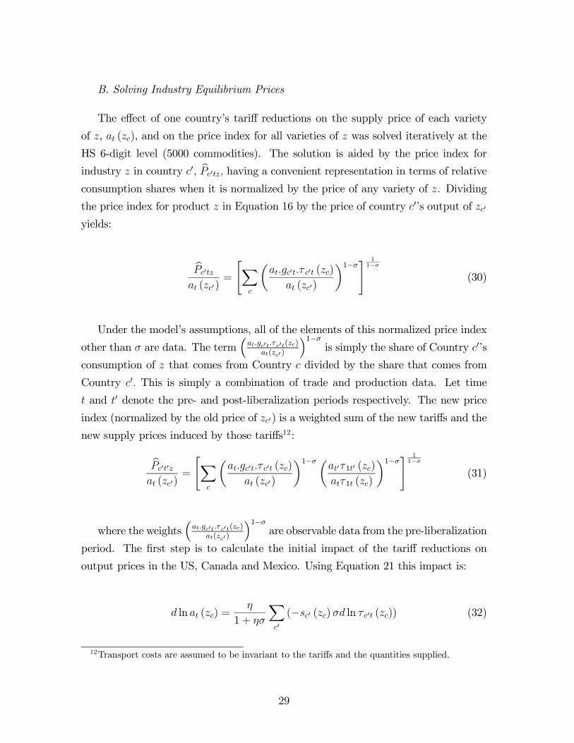
B. Solving Industry Equilibrium Prices
The effect of one country’s tariff reductions on the supply price of each variety
of z, at (zc), and on the price index for all varieties of z was solved iteratively at the
HS 6-digit level (5000 commodities). The solution is aided by the price index for
industry z in country c0, bPc0tz, having a convenient representation in terms of relative
consumption shares when it is normalized by the price of any variety of z. Dividing
the price index for product z in Equation 16 by the price of country c0’s output of zc0
yields:
bPc0tz
at (zc0)=
"Xc
µat.gc0t.τ c0t (zc)
at (zc0)
¶1−σ# 11−σ
(30)
Under the model’s assumptions, all of the elements of this normalized price index
other than σ are data. The term³at.gc0t.τc0t(zc)
at(zc0 )
´1−σis simply the share of Country c0’s
consumption of z that comes from Country c divided by the share that comes from
Country c0. This is simply a combination of trade and production data. Let time
t and t0 denote the pre- and post-liberalization periods respectively. The new price
index (normalized by the old price of zc0) is a weighted sum of the new tariffs and the
new supply prices induced by those tariffs12:
bPc0t0z
at (zc0)=
"Xc
µat.gc0t.τ c0t (zc)
at (zc0)
¶1−σ µat0τ1t0 (zc)atτ1t (zc)
¶1−σ# 11−σ
(31)
where the weights³at.gc0t.τc0t(zc)
at(zc0)
´1−σare observable data from the pre-liberalization
period. The first step is to calculate the initial impact of the tariff reductions on
output prices in the US, Canada and Mexico. Using Equation 21 this impact is:
d ln at (zc) =η
1 + ησ
Xc0(−sc0 (zc) σd ln τ c0t (zc)) (32)
12Transport costs are assumed to be invariant to the tariffs and the quantities supplied.
29

The second step is to use the new tariffs and prices of NAFTA-country output to
compute the change in industry price indexes using Equation 31. The change in the
aggregate price indexes bPct is estimated from the changes in the industry price indexes
using Equation 17, where the expenditure weight bc (z) is estimated consumption of
z in each country or country group c divided by that country’s GDP. The estimated
change in the price indexes can be inserted into Equation 33 to solve for new supply
prices of every variety:
d ln at (zc) =η
1 + ησ
Xc0
³−sc0 (zc)σd ln τ c0t (zc) + sc0 (zc) (σ − 1)d ln bPc0tz
´+
d ln bPct
1 + ησ
(33)
These prices are in turn used to recalculate all price indexes. The price estimates
converge after a few iterations. I then use the fact that in an equilibrium with an
unchanged trade balance, the change in a country’s income equals the change in
expenditures on its output (net of taxes and transport costs) plus the change in taxes
collected on imported goods. The change in quantities demanded are estimated by
substituting the tariff reductions and the changes in goods prices and price indexes
into Equation 20. Changed quantities and prices give changed expenditures on each
country’s output. Changed tariff revenue is calculated using the tariff reductions and
the estimated price and quantity responses. The change in aggregate incomes can be
inserted into Equation 34 to solve for new supply prices of every variety:
d ln at (zc)=η
1 + ησ
Xc0(−sc0 (zc)σd ln τ c0t (zc) + sc0 (zc) (σ − 1)d ln bPc0tz
+sc0 (zc) d lnYc0t) +d ln bPct
1 + ησ(34)
These prices are in turn used to recalculate the price indexes and aggregate in-
comes. This process is iterated until the estimated changes in prices and aggregate
incomes generate no change in the trade balance.
30

C. Additional Data Description for Model Solution
Data is for the year preceding each trade agreement unless unavailable, in which
case the closest year is used. The tariff data used for the US and Canada are applied
tariffs because they are conveniently arranged with the trade data in the Feenstra
database of US trade data and the Canadian trade data from Statistics Canada and
because they capture more nuances of trade policy than the tariff schedules alone.
Tariff schedules are used for Mexico because applied tariffs are unavailable.
sc (zc) : important data for the model are the shares of each country’s output of
each product that are consumed domestically. Production data for US manufacturing
sectors is from the NBER Productivity Database and was merged with US import
and export data at the 4-digit SIC level produced by Feenstra (1996, 1997). US
consumption of US output by industry is calculated as US shipments less US exports.
The estimates of sc (zc) for the US from the SIC data are applied to every 6-digit
HS code that falls within a 4-digit SIC code. Where a 6-digit HS code maps into
more than one SIC code, I use 10-digit HS import data for the US to select the SIC
code that matches the largest amount of trade at the 6-digit level.13 The equivalent
production, import and export data for US non-manufacturing sectors and for Canada
and Mexico at the 2-4-digit ISIC level (depending on product) came from the OECD’s
STAN database and the estimates of sc (zc) are mapped into HS 6-digit codes using
a concordance provided by Mary Amiti of the IMF. sc (zc) for other countries is
estimated simply as the share of each country’s GDP that is not exported to North
America (other countries are combined into the “ROW”).
sc0 (zc) : the share of each country’s output of each product that is consumed by
other countries is calculated using trade data and the estimates of sc (zc). sc0 (zc) is
simply the share of each product that is exported multiplied by the share of exports
that go to country c0:
(1− sc (zc))qc0t (zc)P
c0 6=cqc0t (zc)
(35)
13The 10-digit import data for the US includes a concordance to (import based) SIC.
31

The export shares come from the World Bank’s WITS database at the HS 6-digit
level.
Production at the HS 6-digit level is estimated as exports at the HS 6-digit level
from the WITS database divided by the coarser estimates of the share of each product
that is exported (1− sc (zc)). Consumption at the HS 6-digit level is imports minus
exports from the WITS database plus estimated production.
bc (z) : expenditure weights in the utility functions for each country or country
group, bc (z), is simply the consumption in country c of each HS 6-digit product
(regardless of source) divided by the GDP of that country from the World Bank’s
World Development Indicators.
I set the value of σ at 6 which is close to the median estimate. Higher values of σ
lead to a greater trade volume response but have a small effect on welfare estimates.
The inverse supply elasticity η is taken from the more precisely estimated values in
Table 4 of 0.29.
D. Caveat on Model Results for Mexico
Mexican tariff schedules overstate tariff collection due to duty exemptions for
Maquiladoras. The model therefore overpredicts the decline in Mexican tariff revenues
(which according to the World Bank World Development Indicators were just over 1
percent of GDP in 1993), overpredicts the decline in the Mexican price index, and
overpredicts the increase in the real value of pre-NAFTA output. Without detailed
applied tariff data this can only be addressed with an ad-hoc adjustment to Mexican
tariffs which I have not made. The impact of this caveat on other countries is very
limited. The change in trade resulting from NAFTA is also overstated, but by less
since much of the increase in trade is driven by US tariff reductions which are much
more accurately measured.
32
References
[1] Armington P. (1969), “A Theory of Demand for Products Distinguished by Place
of Production”, IMF Staff Papers 16 (March), pp.159-78.
[2] Arndt, Sven W. (2003), “Global Production Sharing Networks and Regional
Integration”, mimeo, Claremont McKenna College.
[3] Bagwell K. and R. Staiger (1999), “An Economic Theory of GATT”, American
Economic Review, Vol. 89, No.1, pp.215-248.
[4] Baldwin R. (1996), “A Domino Theory of Regionalism”, in Baldwin R., P. Haa-
paranta and J. Kiander eds., Expanding the Membership of the EU, Cambridge
University Press.
[5] Baldwin R.E. and A. J. Venables (1995), “Regional Economic Integration”, in
Grossman G.M. and K. Rogoff eds., Handbook of International Economics, Vol-
ume 3, North-Holland.
[6] Brown D.K., A.V. Deardorff and R.M. Stern (1995), “Estimates of a North
American Free Trade Agreement”, in Kehoe P.J. and Kehoe T.J. (eds.),Modeling
North American Integration, Kluwer Academic Publishers, Dordrecht.
[7] Chang, Won and L. Alan Winters (2002), “How Regional Blocs Affect Excluded
Countries: The Price Effects of MERCOSUR”, American Economic Review,
92(4), pp.889-904.
[8] Clausing K. A. (2001), “Trade Creation and Trade Diversion in the Canada-
United States Free Trade Agreement”, Canadian Journal of Economics, 34(3),
August 2001, pp.677-696.
[9] Cox D.J. (1995), “An Applied General Equilibrium Analysis of NAFTA’s Impact
on Canada”, in Kehoe P.J. and Kehoe T.J. (eds.), Modeling North American
Integration, Kluwer Academic Publishers, Dordrecht.
[10] Deardorff A. and R. Stern (1994), “Multilateral Trade Negotiations and Pref-
erential Trading Arrangements” in A. Deardorff and R. Stern (eds), Analytical
and Negotiating Issues in the Global Trading System, The University of Michigan
Press, Ann Arbor.
[11] Evans, Carolyn L. and James Harrigan (2003); “Tight Clothing: How the MFA
Affects Asian Apparel Exports”, NBERWorking Paper No. 10250, January 2003.
[12] Feenstra Robert C., John Romalis and Peter K. Schott (2002); “U.S. Imports,
Exports, and TariffData, 1989-2001”, NBERWorking Paper No. 9387, December
33

2002.
[13] Frankel J., E. Stein and S. Wei (1996), “Improving the Design of Regional Trade
Agreements. Regional Trading Arrangements: Natural or Supernatural?”, AEA
Papers and Proceedings, Vol. 86, No. 2, pp.52-56.
[14] Fukao K., T. Okubo, and R.M Stern (2003), “An Econometric Analysis of Trade
Diversion under NAFTA”, North American Journal of Economics and Finance,
14(1), March 2003, pp.3-24.
[15] Garces-Diaz D. (2001), “Was NAFTA Behind the Mexican Export Boom (1994-
2000)?”, mimeo (on SSRN), Banco de Mexico, February.
[16] Gould D. (1998), “Has NAFTA Changed North American Trade?”, Federal Re-
serve Bank of Dallas Economic Review, First Quarter, pp.12-22.
[17] Head K. and J. Ries (1999), “Rationalization effects of tariff reductions”, Journal
of International Economics, Vol. 47(2), pp.295—320.
[18] Heckman J. (1976), “The common structure of statistical models of truncation,
sample selection, and limited dependent variables and a simple estimator for such
models”, The Annals of Economic and Social Measurement, Vol. 5, pp.475-492.
[19] Hufbauer G. and J. Schott (1993), NAFTA: An Assessment, (Washington DC,
Institute for International Economics).
[20] Hummels D. (1999), “Have International Trade Costs Declined?”, mimeo.
[21] Kehoe P.J. and Kehoe T.J. (1995), “Capturing NAFTA’s Impact with Applied
General Equilibrium Models”, in Kehoe P.J. and Kehoe T.J. (ed.), Modeling
North American Integration, Kluwer Academic Publishers, Dordrecht.
[22] Kehoe, Timothy J. and Kim J. Ruhl (2002), “How important is the New Goods
Margin in International Trade?”, mimeo, University of Minnesota, October 2002.
[23] Kemp M. and H. Wan (1976), “An Elementary Proposition Concerning the For-
mation of Customs Unions”, Journal of International Economics, Vol. 6, pp.95-
97.
[24] Krueger A. (1999), “Trade Creation and Trade Diversion Under NAFTA”, NBER
Working Paper No. 7429.
[25] Krueger A. (2000), “NAFTA’s Effects: A Preliminary Assessment”,World Econ-
omy, Vol. 23, No.6, pp.761-75.
[26] Levy P. (1997), “A Political-Economic Analysis of Free-Trade Agreements”,
American Economic Review, Vol. 87, No.4, pp.506-519.
[27] Limao Nuno (2003), “Preferential Trade Agreements as Stumbling Blocks for
34

Multilateral Trade Liberalization: Evidence for the U.S.”, mimeo, University of
Maryland, June 2003.
[28] Sobarzo H.E. (1995), “AGeneral EquilibriumAnalysis of the Gains fromNAFTA
for the Mexican Economy”, in Kehoe P.J. and Kehoe T.J. (eds.), Modeling North
American Integration, Kluwer Academic Publishers, Dordrecht.
[29] Trefler D. (2001), “The Long and Short of the Canada-U.S. Free Trade Agree-
ment”, mimeo (on SSRN), University of Toronto, April.
[30] Viner J. (1950), The Customs Union Issue, (New York: Carnegie Endowment).
[31] Wall H. (2000), “NAFTA and the Geography of North American Trade”, mimeo
(on SSRN), Federal Reserve Bank of St. Louis, November.
[32] Yeats A. (1997), “Does Mercosur’s Trade Performance Raise Concerns about the
Effects of Regional Trade Arrangements?”, World Bank Policy ResearchWorking
Paper No. 1729.
[33] Office of the United States Trade Representative (1999), U.S. Generalized System
of Preferences Guidebook, Executive Office of the President, Washington D.C.,
March 1999.
35

Figure 1: Preferential Trade Agreements in Force by Date Notified Source: World Trade Organization
0
20
40
60
80
100
120
140
160
180
200
1958 1963 1968 1973 1978 1983 1988 1993 1998 2003Year
PTA
's in
For
ce
Figure 2: Mexico’s and Canada’s Share of US Imports 1980-2000
0.00
0.05
0.10
0.15
0.20
0.25
1980
1981
1982
1983
1984
1985
1986
1987
1988
1989
1990
1991
1992
1993
1994
1995
1996
1997
1998
1999
2000
Sim
ple
Ave
rage
of S
hare
of U
S Im
port
s by
C
omm
odity
(359
2 co
mm
oditi
es)
0.00
0.02
0.04
0.06
0.08
0.10
Sim
ple
Ave
rage
of S
hare
of U
S Im
port
s by
C
omm
odity
(359
2 co
mm
oditi
es)
Canada (Left Scale)
Mexico (Right Scale)

Figure 3A: Mexico’s Share of US Imports 1989-2000
Figure 3B: Mexico’s Share of EU Imports 1989-2000
Figure 3C: Mexico’s Share of US Imports 1980-2000
0.00
0.02
0.04
0.06
0.08
0.10
0.12
1989 1990 1991 1992 1993 1994 1995 1996 1997 1998 1999 2000Year
Sim
ple
Ave
rage
of S
hare
of U
S Im
port
s by
C
omm
odity
No new US tariff preference (2629 commodities)New US tariff preference >0% and < 10% (1556 commodities)New US tariff preference >= 10% (298 commodities)
0.000
0.002
0.004
0.006
0.008
1989 1990 1991 1992 1993 1994 1995 1996 1997 1998 1999 2000Year
Sim
ple
Ave
rage
of S
hare
of E
U Im
port
s by
C
omm
odity
No new US tariff preference (2629 commodities)New US tariff preference >0% and < 10% (1556 commodities)New US tariff preference >= 10% (298 commodities)
0.00
0.02
0.04
0.06
0.08
0.10
0.12
0.14
1980
1981
1982
1983
1984
1985
1986
1987
1988
1989
1990
1991
1992
1993
1994
1995
1996
1997
1998
1999
2000
Year
Sim
ple
Ave
rage
of S
hare
of U
S Im
port
s by
C
omm
odity
No new tariff preference (2089 commodities)New tariff preference >0% and < 10% (1337 commodities)New tariff preference >= 10% (166 commodities)
1986-2000 GATT/WTO 1994-2000 NAFTA

Figure 4A: Canada’s Share of US Imports 1988-2000
Figure 4B: Canada’s Share of EU Imports 1988-2000
Figure 4C: Canada’s Share of US Imports 1980-2000
0.00
0.05
0.10
0.15
0.20
0.25
1988 1989 1990 1991 1992 1993 1994 1995 1996 1997 1998 1999 2000Year
Sim
ple
Ave
rage
of S
hare
of U
S Im
port
s by
Com
mod
ity
No new US tariff preference (1551 commodities)
New US tariff preference >0% and < 10% (2540 commodities)
New US tariff preference >= 10% (392 commodities)
0.00
0.01
0.02
0.03
0.04
1988 1989 1990 1991 1992 1993 1994 1995 1996 1997 1998 1999 2000Year
Sim
ple
Ave
rage
of S
hare
of E
U Im
port
s by
Com
mod
ity
No new US tariff preference (1551 commodities)New US tariff preference >0% and < 10% (2540 commodities)New US tariff preference >= 10% (392 commodities)
0.00
0.05
0.10
0.15
0.20
0.25
0.30
0.35
1980
1981
1982
1983
1984
1985
1986
1987
1988
1989
1990
1991
1992
1993
1994
1995
1996
1997
1998
1999
2000
Year
Sim
ple
Ave
rage
of S
hare
of U
S Im
port
s by
C
omm
odity
No new tariff preference (1286 commodities)New tariff preference >0% and < 10% (2092 commodities)New tariff preference >= 10% (214 commodities)

Figure 5A: US Import Tariffs in 2000
Figure 5B: US Tariff Preferences for Canadian and Mexican Goods in 2000
0
500
1000
1500
2000
2500
3000
3500
4000
0 1 2 3 4 5 6 7 8 9 10 11 12 13 14 15 16 17 18 19 20 >20
MFN Tariff Rate (%) Less Tariff on Imports from Canada, Mexico
Num
ber o
f HTS
8 C
omm
oditi
es
CanadaMexico

Figure 6: Highly Protected Sectors (A) Effect of CUSFTA/NAFTA (B) Effect of Unilateral Liberalization
Notes: ‘Unilateral Liberalization’ means the dropping of all tariffs by the relevant country. ‘Real Supply Price’ is the output price exclusive of tariffs and transport costs divided by the aggregate price index for that country.
020
4060
80P
erce
nt o
f Hig
hly
Prot
ecte
d Pr
oduc
ts
-10 -5 0 5Percentage Change in Real Supply Price
Highly Protected US Sectors
010
2030
40P
erce
nt o
f Hig
hly
Prot
ecte
d Pr
oduc
ts
-10 -5 0 5 10Percentage Change in Real Supply Price
Highly Protected Canadian Sectors
010
2030
Per
cent
of H
ighl
y Pr
otec
ted
Prod
ucts
-10 -5 0 5 10Percentage Change in Real Supply Price
Highly Protected Mexican Sectors
010
2030
40P
erce
nt o
f Hig
hly
Prot
ecte
d Pr
oduc
ts
-20 -15 -10 -5 0Percentage Change in Real Supply Price
Highly Protected US Sectors
05
1015
2025
Per
cent
of H
ighl
y Pr
otec
ted
Prod
ucts
-20 -15 -10 -5 0Percentage Change in Real Supply Price
Highly Protected Canadian Sectors
010
2030
40P
erce
nt o
f Hig
hly
Prot
ecte
d Pr
oduc
ts
-20 -15 -10 -5 0 5Percentage Change in Real Supply Price
Highly Protected Mexican Sectors

Table 1: Proportion of HTS 8-digit Tariff Variation Captured by Broader Classifications Classification MFN Tariff Canada
Preference Mexico
Preference HS-2 (97 categories) 0.387 0.389 0.370 HS-4 (1258 categories) 0.557 0.573 0.522 HS-6 (5115 categories) 0.684 0.705 0.651
Notes: Table 1 reports the percentages of the variance in US MFN and preferential tariffs at the HTS 8-digit level (10082 products) for the year 1999 that are captured by broader product classifications. Each tariff measure is regressed on full sets of dummy variables for the broader classifications. The R-squared from each regression is reported in Table 1. The 25 products with MFN tariffs above 50 percent are excluded from the calculations.

Table 2A: Tariff Preferences and Relative Prices of US Imports from Canada and Mexico
Year 1999 Tariff Preference (%)
Median Log Relative Price of US Imports from Canada
Median Log Relative Price of US Imports from Mexico
1989 1993 1999 N 1989 1993 1999 N 0 0.082 0.088 0.168 1457 -0.094 0.014 -0.059 663(0,10] 0.154 0.175 0.201 2496 -0.121 -0.033 0.007 1327>10 0.423 0.533 0.602 521 -0.127 0.005 -0.057 234Notes: For each HTS10-digit product the FOB unit price of US imports from Canada, Mexico and the aggregate of all other countries has been calculated for the years 1989, 1993 and 1999. The log price of imports from Canada and Mexico relative to imports from all other countries is then calculated. The median log relative price is then tabulated for 3 arbitrary ranges of tariff preference given by the US to imports from Canada and Mexico. Products are only included if they are imported in all three years. The number of products for each calculation is reported.
Table 2B: Tariff Preferences and Relative Prices of Canadian Imports from US and Mexico
Year 1999 Tariff Preference (%)
Median Log Relative Price of Canadian Imports from US
Median Log Relative Price of Canadian Imports from Mexico
1989 1993 1999 N 1989 1993 1999 N 0 -0.065 -0.036 -0.001 1257 -0.048 -0.011 0.016 76(0,10] 0.018 0.012 0.039 1228 -0.182 0.203 0.126 136>10 0.338 0.391 0.383 706 -0.245 0.269 0.207 36Notes: For each HTS10-digit product the FOB unit price of Canadian imports from the US, Mexico and the aggregate of all other countries has been calculated for the years 1989, 1993 and 1999. The log price of imports from the US and Mexico relative to imports from all other countries is then calculated. The median log relative price is then tabulated for 3 arbitrary ranges of tariff preference given by Canada to imports from the US and Mexico. Products are only included if they are imported in all three years. The number of products for each calculation is reported. Table 2C: Tariff Preferences and Relative Prices of Mexican Imports from US and Canada
Year 1999 Tariff Preference (%)
Median Log Relative Price of Mexican Imports from US
Median Log Relative Price of Mexican Imports from Canada
1989 1993 1999 N 1989 1993 1999 N [0,10] - -0.226 -0.263 1547 - 0.002 0.105 640(10,20] - -0.257 -0.441 2081 - 0.098 0.037 813>20 - -0.076 0.000 709 - 0.426 0.464 232Notes: For each HS 6-digit product the FOB unit price of Mexican imports from the US, Canada, and the aggregate of all other countries has been calculated for the years 1993 and 1999 (1989 data being unavailable). The log price of imports from the US and Canada relative to imports from all other countries is then calculated. The median log relative price is then tabulated for 3 arbitrary ranges of tariff preference given by Mexico to imports from the US and Canada. These tariff ranges differ from Tables 2A and 2B because there are almost no observations where the preference is zero. Products are only included if they are imported in both years. The number of products for each calculation is reported.

Table 3A: Substitution Elasticity Estimates based on US and EU Imports from Canada and Control Countries, 1989-1999
(1) (2) (3) (4) (5) (6) (7) (8)
σ 6.52 (0.80)
6.68 (0.90)
9.38 (0.88)
8.73 (1.06)
6.25 (0.77)
6.30 (0.85)
8.49 (0.84)
7.72 (0.97)
Commodity Fixed Effects Yes Yes Yes Yes Yes Yes Yes Yes
Year Fixed Effects Yes Yes Yes Yes Yes Yes Yes Yes
Control Countries Table A1 Table A1 Table A1 Table A1 All All All All
Tariff Measure
Schedule; import
weighted
Schedule; simple average
Applied; import
weighted
Applied;simple average
Schedule; import
weighted
Schedule; simple average
Applied; import
weighted
Applied; simple average
N 35537 35533 35536 35532 36089 36085 36088 36084 Commodities 4631 4631 4631 4631 4694 4694 4694 4694
Notes: Dependent variable is ln(US imports from Canada/US imports from control countries) - ln(EU12 imports from Canada/EU12 imports from control countries) by year and HS 6-digit commodity. The substitution elasticity estimate comes from regressions of this variable on a measure of the tariff preference that the US gives to goods of Canadian origin. The EU12 includes the 12 countries that were members of the EU in 1989. The “Table A1” control countries are listed in Appendix Table A1. When “All” countries are used as a control, this includes all countries (including intra-EU international trade) with the exception of NAFTA countries. Robust standard errors adjusted for clustering on each commodity are in parentheses. There is a small difference between the number of observations in columns for the same set of control countries because a small number of observations with extreme values for the calculated tariff preference (where ln(1+preference) is greater than 0.5) are discarded.
Table 3B: Substitution Elasticity Estimates based on US and EU Imports from Mexico and Control Countries, 1989-1999
(1) (2) (3) (4) (5) (6) (7) (8)
σ 9.90 (1.02)
10.15 (1.15)
10.90 (1.19)
9.59 (1.25)
9.88 (1.00)
10.04 (1.08)
10.88 (1.16)
9.61 (1.20)
Commodity Fixed Effects Yes Yes Yes Yes Yes Yes Yes Yes
Year Fixed Effects Yes Yes Yes Yes Yes Yes Yes Yes
Control Countries Table A1 Table A1 Table A1 Table A1 All All All All
Tariff Measure
Schedule; import
weighted
Schedule; simple average
Applied; import
weighted
Applied; simple average
Schedule; import
weighted
Schedule; simple average
Applied; import
weighted
Applied; simple average
N 19335 19335 19334 19333 19414 19414 19413 19412 Commodities 3415 3415 3415 3415 3427 3427 3427 3427
Notes: Dependent variable is ln(US imports from Mexico/US imports from control countries) - ln(EU12 imports from Mexico/EU12 imports from control countries) by year and HS 6-digit commodity. The substitution elasticity estimate comes from regressions of this variable on a measure of the tariff preference that the US gives to goods of Mexican origin. The EU12 includes the 12 countries that were members of the EU in 1989. The “Table A1” control countries are listed in Appendix Table A1. When “All” countries are used as a control, this includes all countries (including intra-EU international trade) with the exception of NAFTA countries. Robust standard errors adjusted for clustering on each commodity are in parentheses. There is a small difference between the number of observations in columns for the same set of control countries because a small number of observations with extreme values for the calculated tariff preference (where ln(1+preference) is greater than 0.5) are discarded.

Table 3C: Substitution Elasticity Estimates based on Canadian and EU Imports from USA and Control Countries, 1989-1999
(1) (2) (3) (4) (5) (6) (7) (8)
σ 5.51 (0.47)
5.07 (0.45)
2.99 (0.44)
2.84 (0.46)
5.31 (0.42)
4.96 (0.41)
3.09 (0.39)
2.95 (0.39)
Commodity Fixed Effects Yes Yes Yes Yes Yes Yes Yes Yes
Year Fixed Effects Yes Yes Yes Yes Yes Yes Yes Yes
Control Countries Table A1 Table A1 Table A1 Table A1 All All All All
Tariff Measure
Applied; import
weighted
Applied; simple average
Schedule; import
weighted
Schedule; simple average
Applied; import
weighted
Applied; simple average
Schedule; import
weighted
Schedule; simple average
N 44280 44277 44278 44278 49038 49035 49038 49038 Commodities 5150 5150 5150 5150 5242 5242 5242 5242 Notes: Dependent variable is ln(Canadian imports from US/Canadian imports from control countries) - ln(EU12 imports from US/EU12 imports from control countries) by year and HS 6-digit commodity. The substitution elasticity estimate comes from regressions of this variable on a measure of the tariff preference that Canada gives to goods of US origin. The EU12 includes the 12 countries that were members of the EU in 1989. The “Table A1” control countries are listed in Appendix Table A1. When “All” countries are used as a control, this includes all countries (including intra-EU international trade) with the exception of NAFTA countries. Robust standard errors adjusted for clustering on each commodity are in parentheses. There is a small difference between the number of observations in columns for the same set of control countries because a small number of observations with extreme values for the calculated tariff preference (where ln(1+preference) is greater than 0.5) are discarded.
Table 3D: Substitution Elasticity Estimates based on Canadian and EU Imports from Mexico and Control Countries, 1989-1999
(1) (2) (3) (4) (5) (6) (7) (8)
σ 8.06 (1.14)
7.85 (1.16)
6.80 (1.24)
7.32 (1.31)
7.64 (1.10)
7.20 (1.14)
6.63 (1.19)
7.02 (1.28)
Commodity Fixed Effects Yes Yes Yes Yes Yes Yes Yes Yes
Year Fixed Effects Yes Yes Yes Yes Yes Yes Yes Yes
Control Countries Table A1 Table A1 Table A1 Table A1 All All All All
Tariff Measure
Applied; import
weighted
Applied; simple average
Schedule; import
weighted
Schedule; simple average
Applied; import
weighted
Applied; simple average
Schedule; import
weighted
Schedule; simple average
N 13137 13137 13139 13139 13219 13219 13220 13220 Commodities 2674 2674 2674 2674 2695 2695 2695 2695
Notes: Dependent variable is ln(Canadian imports from Mexico/Canadian imports from control countries) - ln(EU12 imports from Mexico/EU12 imports from control countries) by year and HS 6-digit commodity. The substitution elasticity estimate comes from regressions of this variable on a measure of the tariff preference that Canada gives to goods of Mexican origin. The EU12 includes the 12 countries that were members of the EU in 1989. The “Table A1” control countries are listed in Appendix Table A1. When “All” countries are used as a control, this includes all countries (including intra-EU international trade) with the exception of NAFTA countries. Robust standard errors adjusted for clustering on each commodity are in parentheses. There is a small difference between the number of observations in columns for the same set of control countries because a small number of observations with extreme values for the calculated tariff preference (where ln(1+preference) is greater than 0.5) are discarded.

Table 3E: Substitution Elasticity Estimates based on Mexican and EU Imports from USA, Canada and Control Countries, 1990-1999
(1) (2) (3) (4)
σ 2.50 (0.48)
1.98 (0.41)
0.77 (0.88)
0.56 (0.82)
Commodity Fixed Effects Yes Yes Yes Yes
Year Fixed Effects Yes Yes Yes Yes
Imports from USA/Canada USA USA Canada Canada
Control Countries Table A1 All Table A1 All
Tariff Measure Schedule;
simple average
Schedule; simple average
Schedule; simple average
Schedule; simple average
N 38002 42457 19692 20314 Commodities 4684 4844 3430 3524
Notes: Dependent variable in columns 1-2 is ln(Mexican imports from US/Mexican imports from control countries) - ln(EU12 imports from US/EU12 imports from control countries) by year and HS 6-digit commodity. Dependent variable in columns 3-4 is ln(Mexican imports from Canada/Mexican imports from control countries) - ln(EU12 imports from Canada/EU12 imports from control countries) by year and HS 6-digit commodity. The substitution elasticity estimate comes from regressions of the dependent variable on a measure of the tariff preference that Mexico gives to goods of US or Canadian origin. The EU12 includes the 12 countries that were members of the EU in 1989. The “Table A1” control countries are listed in Appendix Table A1. When “All” countries are used as a control, this includes all countries (including intra-EU international trade) with the exception of NAFTA countries. Robust standard errors adjusted for clustering on each commodity are in parentheses. A small number of observations with extreme values for the calculated tariff preference (where ln(1+preference) is greater than 0.5) are discarded.

Table 4: Inverse Supply Elasticity Estimates 1989-1999 (1)
IV (2) IV
(3) IV
(4) OLS
η 0.29 (0.02)
0.29 (0.02)
0.22 (0.04)
-0.31 (0.00)
Commodity x Country Fixed Effects Yes Yes Yes Yes
Year x Country Fixed Effects Yes Yes Yes Yes
Estimation Technique IV IV IV OLS Instruments (see notes) Set 1 Set 2 Set 3 - N 1,099,097 1,099,097 1,099,097 1,099,097
Notes: the dependent variable is the observed FOB unit price of each country’s exports in HS 10-digit US import data. This is regressed on an estimate of the total quantity produced of each product by each exporting country. That quantity estimate is produced using: the quantity exported to the US at the 10-digit level; the share of each country’s exports at the HS 6-digit level that are exported to the US; and the share of each country’s GDP that is exported. Four US tariff measures are used as instruments for the (estimated) quantity: US tariff rates on exports from the exporting country, Canada, Mexico, and all other countries. Instrument “Set 1” includes all these tariffs; “Set 2” only includes the tariff on exports from the exporting country; and “Set 3” includes the tariffs on exports from Canada, Mexico, and all other countries. Standard errors are reported in parentheses.

Tab
le 5
: Tra
de D
iver
sion
infe
rred
from
Nor
th A
mer
ican
and
EU
Impo
rts f
rom
Con
trol
Cou
ntri
es (c
’)
(1
) (2
) (3
) (4
) (5
) (6
) (7
) (8
)
T
rade
D
iver
sion
2.
84
{0.0
00}
2.96
{0
.000
} 3.
37
{0.0
00}
3.87
{0
.000
} 1.
44
{0.0
04}
1.33
{0
.009
} 2.
23
{0.0
00}
2.11
{0
.000
}
Tarif
f
ln
τU
S-C
an
0.06
(0
.93)
0.
34
(0.8
2)
0.49
(0
.54)
0.
40
(0.5
3)
-0.7
1 (0
.75)
-0
.69
(0.8
1)
0.24
(0
.37)
0.
06
(0.4
2)
ln τ
US-
Mex
1.
27
(0.6
0)
1.30
(0
.57)
1.
44
(0.4
4)
1.38
(0
.45)
1.
26
(0.4
9)
1.41
(0
.48)
0.
90
(0.3
4)
0.98
(0
.33)
ln τ
Can
-US
2.02
(0
.52)
1.
91
(0.5
4)
1.26
(0
.45)
1.
75
(0.4
7)
0.19
(0
.35)
0.
11
(0.3
7)
0.26
(0
.34)
0.
44
(0.3
0)
ln τ
Can
-Mex
-0
.95
(0.4
2)
-1.0
0 (0
.44)
-0
.30
(0.2
9)
-0.0
7 (0
.57)
0.
33
(0.3
2)
0.08
(0
.30)
0.
42
(0.2
4)
0.38
(0
.23)
ln τ
Mex
-US
-1.3
2 (0
.55)
-1
.31
(0.5
4)
-1.1
0 (0
.50)
-1
.21
(0.5
1)
-0.6
1 (0
.42)
-0
.61
(0.4
1)
-0.4
8 (0
.38)
-0
.54
(0.3
8)
ln τ
Mex
-Can
1.
76
(0.5
5)
1.71
(0
.55)
1.
57
(0.5
1)
1.61
(0
.52)
0.
98
(0.4
2)
1.03
(0
.43)
0.
89
(0.3
8)
0.96
(0
.39)
MFN
Tar
iffs
Yes
Y
es
Yes
Y
es
Yes
Y
es
Yes
Y
es
Com
mod
ity
Fixe
d Ef
fect
s Y
es
Yes
Y
es
Yes
Y
es
Yes
Y
es
Yes
Yea
r Fix
ed
Effe
cts
Yes
Y
es
Yes
Y
es
Yes
Y
es
Yes
Y
es
Con
trol
Cou
ntrie
s Ta
ble
A1
Tabl
e A
1 Ta
ble
A1
Tabl
e A
1 A
ll A
ll A
ll A
ll
Tarif
f M
easu
re
Sche
dule
; im
port
wei
ghte
d
Sche
dule
; si
mpl
e av
erag
e
App
lied;
im
port
wei
ghte
d
App
lied;
si
mpl
e av
erag
e
Sche
dule
; im
port
wei
ghte
d
Sche
dule
; si
mpl
e av
erag
e
App
lied;
im
port
wei
ghte
d
App
lied;
si
mpl
e av
erag
e
N
4263
0 42
454
4273
4 42
447
4375
6 43
633
4393
0 43
626
Com
mod
ities
53
12
5313
53
21
5313
53
49
5345
53
54
5345
N
otes
: Dep
ende
nt v
aria
ble
is ln
(Nor
th A
mer
ican
impo
rts fr
om c
ontro
l cou
ntrie
s) -
ln(E
U12
impo
rts fr
om c
ontro
l cou
ntrie
s) b
y ye
ar a
nd H
S 6-
digi
t com
mod
ity, w
here
N
orth
Am
eric
a is
the
sum
of t
he U
S, C
anad
a an
d M
exic
o. T
he E
U12
incl
udes
the
12 c
ount
ries t
hat w
ere
mem
bers
of t
he E
U in
198
9. T
he d
epen
dent
var
iabl
e is
re
gres
sed
on m
easu
res o
f the
tarif
fs th
at N
orth
Am
eric
an c
ount
ries l
evy
on g
oods
from
with
in N
orth
Am
eric
a an
d on
the
MFN
tarif
fs o
f the
US,
Can
ada,
Mex
ico
and
the
EU. F
or e
xam
ple,
τU
S-C
an is
the
tarif
f tha
t the
US
levi
es o
n go
ods f
rom
Can
ada
plus
1. T
he fi
rst r
ow “
Trad
e D
iver
sion
” re
ports
the
sum
of t
he c
oeff
icie
nts o
n ta
riffs
le
vied
by
Nor
th A
mer
ican
cou
ntrie
s on
impo
rts fr
om th
eir N
AFT
A p
artn
ers (
the
six
coef
ficie
nts r
epor
ted
belo
w) –
the
p-va
lue
for t
he te
st th
at th
is su
m is
zer
o is
re
porte
d in
bra
ces.
A si
gnifi
cant
pos
itive
num
ber i
s evi
denc
e of
trad
e di
vers
ion
resu
lting
from
pre
fere
ntia
l tar
iffs.
The
“Tab
le A
1” c
ontro
l cou
ntrie
s are
list
ed in
A
ppen
dix
Tabl
e A
1. W
hen
“All”
cou
ntrie
s are
use
d as
a c
ontro
l, th
is in
clud
es a
ll co
untri
es (i
nclu
ding
intra
-EU
inte
rnat
iona
l tra
de) w
ith th
e ex
cept
ion
of N
AFT
A
coun
tries
. Rob
ust s
tand
ard
erro
rs a
djus
ted
for c
lust
erin
g on
eac
h co
mm
odity
are
in p
aren
thes
es. T
here
is a
smal
l diff
eren
ce b
etw
een
the
num
ber o
f obs
erva
tions
in
colu
mns
for t
he sa
me
set o
f con
trol c
ount
ries b
ecau
se a
smal
l num
ber o
f obs
erva
tions
with
ext
rem
e va
lues
of t
he c
alcu
late
d ta
riff (
whe
re ln
(1+t
ariff
) exc
eeds
0.5
) are
di
scar
ded.
Dat
a on
act
ual d
utie
s col
lect
ed is
not
ava
ilabl
e fo
r Mex
ico
so re
gres
sion
s alw
ays i
nclu
de th
e M
exic
an ta
riff s
ched
ule.
Sin
ce M
exic
an ta
riffs
on
US
and
Can
adia
n go
ods a
re v
ery
sim
ilar t
he se
para
te e
ffec
ts o
f the
se tw
o ta
riffs
may
diff
icul
t to
empi
rical
ly d
isen
tang
le.

Table 6: Model Results
Change in Welfare due to CUSFTA (% of GDP)
CountryReal Value of
Existing OutputReal Tariff Revenue Welfare
USA 0.01 -0.02 -0.01Canada 0.28 -0.28 0.00Mexico 0.00 0.00 0.00Rest of World 0.00 - 0.00See text for an explanation of the decomposition
Change in Welfare due to NAFTA (% of GDP)
CountryReal Value of
Existing OutputReal Tariff Revenue Welfare
USA 0.03 -0.03 0.00Canada 0.02 -0.02 0.00Mexico* 1.09 -1.39 -0.30Rest of World 0.00 - 0.00*See Appendix for a caveat on Mexican results.See text for an explanation of the decomposition.
Change In Bilateral Trade Due to CUSFTA (billions 1988 USD \ %)Partners USA Canada Mexico ROWUSA 5.35% 0.08% 0.11%Canada 8.32 -2.38% -0.49%Mexico 0.04 -0.05 0.01%ROW 0.64 -0.32 0.00Note: Elements below principal diagonal are in billions of 1988 USD, other elements are percentage changes.
Change In Bilateral Trade Due to NAFTA (billions 1993 USD \ %)Partners USA Canada Mexico ROWUSA -0.17% 23.38% -0.34%Canada -0.34 23.74% -0.49%Mexico 18.47 0.81 -9.58%ROW -2.48 -0.32 -1.97Note: Elements below principal diagonal are in billions of 1993 USD, other elements are percentage changes.

Appendix Table 1Countries with no substantial change in preferential trade relations with the EUAfghanistan Gabon Norfolk IsAngola Gambia North KoreaAntigua Barbuda Ghana NorwayArgentina Greenland OmanAruba Grenada Is PakistanAustralia Guatemala PalauBahamas Guinea PanamaBahrain Guinea-Bissau Papua New GuinBangladesh Guyana ParaguayBarbados Haiti PeruBelize Honduras PhilippinesBenin Hong Kong Pitcairn IsBermuda India QatarBhutan Indonesia RwandaBolivia Iran SamoaBotswana Jamaica Saudi ArabiaBrazil Japan SenegalBrunei Kenya SeychellesBurkina Faso Kiribati Sierra LeoneBurundi Korea SingaporeCambodia Laos Solomon IsCameroon Lesotho SomaliaCape Verde Liberia Sri LankaCayman Is Libya St Kitts-NevisCen African Rep Macao St Lucia IsChad Madagascar St Vinc & GrenChile Malawi SudanChina Malaysia SurinameChristmas Is Maldive Is SwazilandCocos Is Mali SwitzerlandColombia Marshall Is TaiwanComoros Mauritania TanzaniaCongo (DROC) Mauritius ThailandCongo (ROC) Mongolia TogoCook Is Montserrat Is TongaCosta Rica Mozambique Trin & TobagoCote d'Ivoire Namibia TuvaluCuba Nauru UgandaDjibouti Nepal United Arab EmDominica Is Netherlands Ant UruguayDominican Rep New Caledonia VenezuelaEcuador New Zealand VietnamEl Salvador Nicaragua YemenEq Guinea Niger ZambiaEthiopia Nigeria ZimbabweFiji Niue

App
endi
x T
able
2: S
ubst
itutio
n E
last
icity
Est
imat
es w
hen
Con
trol
Cou
ntri
es a
re n
ot A
ggre
gate
d, 1
989-
1999
(1)
(2)
(3)
(4)
(5)
(6)
(7)
(8)
(9)
(10)
(1
1)
(12)
Im
porti
ng
Cou
ntry
U
SA
USA
U
SA
USA
C
anad
a C
anad
a C
anad
a C
anad
a M
exic
o M
exic
o M
exic
o M
exic
o
σ 5.
50
(0.2
5)
5.26
(0
.17)
7.
83
(0.3
1)
6.72
(0
.21)
3.
23
(0.2
1)
3.12
(0
.13)
5.
01
(0.3
6)
4.80
(0
.24)
2.
80
(0.2
7)
2.50
(0
.17)
1.
99
(0.4
2)
2.16
(0
.29)
C
omm
odity
x
Con
trol C
ount
ry
Fixe
d Ef
fect
s Y
es
Yes
Y
es
Yes
Y
es
Yes
Y
es
Yes
Y
es
Yes
Y
es
Yes
Yea
r Fix
ed
Effe
cts
Yes
Y
es
Yes
Y
es
Yes
Y
es
Yes
Y
es
Yes
Y
es
Yes
Y
es
Pref
erre
d C
ount
ry
Can
ada
Can
ada
Mex
ico
Mex
ico
USA
U
SA
Mex
ico
Mex
ico
USA
U
SA
Can
ada
Can
ada
Con
trol C
ount
ries
Tabl
e A
1 A
ll Ta
ble
A1
All
Tabl
e A
1 A
ll Ta
ble
A1
All
Tabl
e A
1 A
ll Ta
ble
A1
All
Tarif
f Mea
sure
A
pplie
d;
impo
rt w
eigh
ted
App
lied;
im
port
wei
ghte
d
App
lied;
im
port
wei
ghte
d
App
lied;
im
port
wei
ghte
d
App
lied;
im
port
wei
ghte
d
App
lied;
im
port
wei
ghte
d
App
lied;
im
port
wei
ghte
d
App
lied;
im
port
wei
ghte
d
Sche
dule
; si
mpl
e av
erag
e
Sche
dule
; si
mpl
e av
erag
e
Sche
dule
; si
mpl
e av
erag
e
Sche
dule
; si
mpl
e av
erag
e N
33
1993
74
3763
24
1892
51
4474
26
9207
58
9519
15
0356
30
6060
16
9278
37
7015
12
8734
27
7266
C
omm
oditi
es x
C
ontro
l Cou
ntrie
s 62
607
1375
20
5177
1 10
9596
56
578
1221
29
3933
7 81
109
4408
7 94
176
3639
2 76
180
Not
es: D
epen
dent
var
iabl
e is
ln(im
porti
ng c
ount
ry im
ports
from
pre
ferr
ed c
ount
ry/im
porti
ng c
ount
ry im
ports
from
con
trol c
ount
ry) -
ln(E
U12
impo
rts fr
om p
refe
rred
co
untry
/EU
12 im
ports
from
con
trol c
ount
ry) b
y ye
ar a
nd H
S 6-
digi
t com
mod
ity a
nd c
ontro
l cou
ntry
. The
subs
titut
ion
elas
ticity
esti
mat
e co
mes
from
regr
essi
ons o
f th
is v
aria
ble
on a
mea
sure
of t
he ta
riff p
refe
renc
e th
at th
e im
porti
ng c
ount
ry g
ives
to g
oods
from
the
pref
erre
d co
untry
. The
EU
12 in
clud
es th
e 12
cou
ntrie
s tha
t wer
e m
embe
rs o
f the
EU
in 1
989.
The
“Ta
ble
A1”
con
trol c
ount
ries a
re li
sted
in A
ppen
dix
Tabl
e A
1. W
hen
“All”
cou
ntrie
s are
use
d as
a c
ontro
l, th
is in
clud
es a
ll co
untri
es
(incl
udin
g in
tra-E
U in
tern
atio
nal t
rade
) with
the
exce
ptio
n of
NA
FTA
cou
ntrie
s. R
obus
t sta
ndar
d er
rors
adj
uste
d fo
r clu
ster
ing
on e
ach
com
mod
ity*C
ontro
l Cou
ntry
ar
e in
par
enth
eses
. Obs
erva
tions
with
ext
rem
e va
lues
for t
he c
alcu
late
d ta
riff p
refe
renc
e (w
here
ln(1
+pre
fere
nce)
is g
reat
er th
an 0
.5) a
re d
isca
rded
. Mex
ican
impo
rt da
ta is
onl
y av
aila
ble
from
199
0 on
war
ds.