Embed Size (px)
Citation preview
NBER WORKING PAPER SERIES
INFLATION DYNAMICS:A STRUCTURAL ECONOMETRIC ANALYSIS
Jordi GalíMark Gertler
Working Paper 7551http://www.nber.org/papers/w7551
NATIONAL BUREAU OF ECONOMIC RESEARCH1050 Massachusetts Avenue
Cambridge, MA 02138February 2000
The authors thank participants at the JME-SNB Gerzensee Conference on “The Return of the Phillips Curve,NBER Summer Institute and ME Meetings, and seminars at Lausanne, UPF, Delta, Chicago, Michigan,Princeton, Yale, Columbia, San Francisco Fed, BIS, IIES, and the ECB, for useful comments. Special thanksalso to John Roberts and Mark Watson. Tomasso Monacelli and Fabio Natalucci provided excellent researchassistance. Financial support from the C.V. Starr Center for Applied Economics, the National ScienceFoundation, and CREI is gratefully acknowledged. The views expressed herein are those of the authors andnot necessarily those of the National Bureau of Economic Research.
© 2000 by Jordi Galí and Mark Gertler. All rights reserved. Short sections of text, not to exceed twoparagraphs, may be quoted without explicit permission provided that full credit, including © notice, is givento the source.
Inflation Dynamics: A Structural Econometric AnalysisJordi Galí and Mark GertlerNBER Working Paper No. 7551February 2000JEL No. E31
ABSTRACT
We develop and estimate a structural model of inflation that allows for a fraction of firms that use
a backward looking rule to set prices. The model nests the purely forward looking New Keynesian Phillips
curve as a particular case. We use measures of arginal cost as the relevant determinant of inflation, as the
theory suggests, instead of an ad-hoc output gap. Real marginal costs are a significant and quantitatively
important determinant of inflation. Backward looking price setting, while statistically significant, is not
quantitatively important. Thus, we conclude that the New Keynesian Phillips curve provides a good first
approximation to the dynamics of inflation.
Jordi Galí Mark GertlerDepartment d’Economia Department of EconomicsUniversitat Pompeu Fabra New York UniversityRamon Trias Fargas 25 269 Mercer Street, 7th Floor08005 Barcelona New York, NY 10003Spain and NBERand NBER, and New York University [email protected] [email protected]
1 Introduction
Among the central issues in macroeconomics is the nature of short run inflationdynamics. This matter is also one of the most fiercely debated, with few definitiveanswers available after decades of investigation. At stake, among other things, is thenature of business cycles and what should be the appropriate conduct of monetarypolicy.1
In response to this challenge, important advances have emerged recently in thetheoretical modeling of inflation dynamics.2 This new literature builds on early workby Fischer (1977), Taylor (1980), Calvo (1983) and others that emphasized stag-gered nominal wage and price setting by forward looking individuals and firms. Itextends this work by casting the price setting decision within an explicit individualoptimization problem. Aggregating over individual behavior then leads, typically, toa relation that links inflation in the short run to some measure of overall real activity,in the spirit of the traditional Phillips curve. The explicit use of microfoundations, ofcourse, places additional structure on the relation and also leads to some importantdifferences in details.
Despite the advances in theoretical modeling, accompanying econometric analysisof the “new Phillips curve” has been rather limited, though with a few notable excep-tions.3 The work to date has generated some useful findings, but these findings havealso raised some troubling questions about the existing theory. As we discuss below,it appears difficult for these models to capture the persistence in inflation without ap-pealing either to some form of stickiness in inflation that is hard to motivate explicitlyor to adaptive expectations, which also poses difficulty from a modeling standpoint.In addition, with quarterly data, it is often difficult to detect a statistically significanteffect of real activity on inflation using the structural formulation implied by theory,when the measure of real activity is an output gap (i.e., real output relative to somemeasure of potential output). Failure to find a significant short run link between realactivity and inflation is obviously unsettling for the basic story.
In this context, we develop and estimate a structural model of the Phillips curve.Our approach has three distinctive features. First, in the empirical implementation,we use a measure of real marginal cost in place of an ad hoc output gap, as the theorysuggests. As will become apparent, a desirable feature of a marginal cost measureis that it directly accounts for the impact of productivity gains on inflation, a factor
1For recent work that explores how the appropriate course of monetary policy depends on thenature of short run inflation dynamics, see Svensson (1997a, 1997b), Clarida, Gali and Gertler(1997b), Rotemberg andWoodford (1997b), McCallum and Nelson (1998), King andWolman (1998),and Erceg, Henderson and Levin (1998).
2See Goodfriend and King (1997) for a comprehensive survey.3Examples of work that attempts to estimate the new Phillips curve include, Chada, Masson
and Meredith (1992), Fuhrer and Moore (1995), Fuhrer (1997), and Roberts (1997, 1998). Fordiscussions of the traditional empirical literature on the Phillips curve, see King and Watson (1994),Gordon (1996) and Lown and Rich (1997).
1
that simple output gap measures often miss. In this respect, our approach is comple-mentary to Sbordone (1998), though she uses a different methodology to empiricalassess the model than we do.4 Second, we extend the baseline theory underlyingthe new Phillips curve to allow for a subset of firms that set prices according to abackward looking rule of thumb. Doing so allows us to directly estimate the degreeof departure from a pure forward looking model needed to account for the observedinflation persistence. Third, we identify and estimate all the structural parameters ofthe model using conventional econometric methods. The coefficients in our structuralinflation equation are “mongrel” functions of two key model primitives: the averageduration that an individual price is fixed (i.e., the degree of price “stickiness”) and thefraction of firms that use rule of thumb behavior (i.e., the degree of “backwardness”).
As we show, several results stand out and appear to be quite robust: (a) Realmarginal costs are indeed a statistically significant and quantitatively important de-terminant of inflation, as the theory predicts; (b) Forward looking behavior is veryimportant: our model estimates suggest that roughly sixty to eighty percent of firmsexhibit forward looking price setting behavior; (c) Backward looking behavior is sta-tistically significant though, in our preferred specifications, is of limited quantitativeimportance. Thus, while the benchmark pure forward looking model is rejected onstatistical grounds, it appears still to be a reasonable first approximation of reality;(d) The average duration a price is fixed is considerable, but the estimates are in linewith survey evidence.
Taken as whole, our results are supportive of the new, theory-based Phillips curves.But they also raise a puzzle. Traditional explanations of inertia in inflation (and hencethe costs of disinflations) rely on some form of “backwardness” in price setting. Tothe extent this backwardness is not quantitatively important, as we seem to find,the story needs to be re-examined. In our view, the “black box” to investigate isthe link between aggregate activity and real marginal costs. To the extent they arereasonably characterized by unit labor costs, real marginal costs tend to lag outputover the cycle rather than move contemporaneously, in contrast to the prediction ofthe standard sticky price macroeconomic framework.5 In this respect, our analysissuggests that a potential source of inflation inertia may be sluggish adjustment ofreal marginal costs to movements in output. We elaborate on this possibility in theconclusion.
4Sbordone (1998) explores how well the model fits the data conditional on different choices ofa parameter that governs the degree of price rigidity. Our approach is to directly estimate thestructural parameters using an instrumental variables procedure that is based on the orthogonalityconditions that evolve from the underlying theory. In addition, we develop a general model thatnests the pure forward looking model as a special case. Doing so allows us to test directly thedeparture from the pure forward looking model that is required to explain the data. Despite thesharp differences in methodology, the main conclusions we draw are very similar to hers, as wediscuss later.
5Christiano, Eichenbaum and Evans (1997) also stress that the standard sticky price frameworkdoes not seem to explain the cyclical behavior of marginal cost.
2

The paper proceeds as follows: Section 2 reviews the basic theory underlying thenew Phillips curve and discusses the existing empirical literature. We make clearwhy specifications based on the output gap are likely to be unsuccessful. Section 3then presents estimates of the new Phillips curve using a measure of real marginalcost, and shows that with this specification the theory does a reasonably good job ofdescribing the data. To explore further the issue of how well the theory captures theinertia in inflation, section 4 extends the model to allow for a subset of firms that userule of thumb behavior. It then presents estimates of the resulting augmented Phillipscurve and a variety of robustness exercises. In addition, we construct a measure of“fundamental inflation” based on the solution to the estimated model that relatesinflation to a discounted stream of expected future marginal costs, as well as laggedinflation. We in turn show that this measure does a good job of describing the actualpath of inflation, including the recent period. Section 5 concludes.
2 The New Phillips Curve: Background Theory
and Evidence
In this section we review the recent theory that generates an estimable Phillips curverelation. We then discuss some of the pitfalls involved in estimating this relationand how the literature has dealt with these issues to date. Finally, we describe ourapproach.
2.1 A Baseline Model
The typical starting point for the derivation of the new Phillips curve is an envi-ronment of monopolistically competitive firms that face some type of constraints onprice adjustment. In the most common incarnations, the constraint is that the priceadjustment rule is time dependent. For example, every period the fraction 1
Xof firms
set their prices forX periods. The scenario is in the spirit of Taylor’s (1980) staggeredcontracts model. A key difference is that the pricing decision evolves explicitly froma monopolistic competitor’s profit maximization problem, subject to the constraintof time dependent price adjustment.
In general, however, aggregation is cumbersome with deterministic time dependentpricing rules at the micro level: It is necessary to keep track of the price histories offirms. For this reason, it is common to employ an assumption due to Calvo (1983)that greatly simplifies the aggregation problem.6 The idea is to assume that in any
6Examples of frameworks that employ the Calvo assumption include Yun (1996), King and Wol-man (1995), Woodford (1996), Rotemberg and Woodford (1997a, 1997b), Clarida, Gali and Gertler(1997a), McCallum and Nelson (1998), and Bernanke, Gertler and Gilchrist (1998). For a gen-eral equilibrium sticky price model based on the Taylor (1980) formulation, see Chari, Kehoe andMcGratten (1996) and Kiley (1997).
3

given period each firm has a fixed probability 1−θ that it may adjust its price duringthat period and, hence, a probability θ that it must keep its price unchanged. Thisprobability is independent of the time elapsed since the last price revision. Hence, theaverage time over which a price is fixed is given by (1− θ)
∑∞
k=0 kθk−1 = 1
1−θ. Thus,
for example, with θ = .75 in a quarterly model, prices are fixed on average for a year.Because the adjustment probabilities are independent of the firm’s price history, theaggregation problem is greatly simplified.
We can derive the new Phillips curve by proceeding as follows7: Assume that firmsare identical ex ante, except for the differentiated product they produce and for theirpricing history. Assume also that each faces a conventional constant price elasticityof demand curve for its product. Then it is possible to show that the aggregate pricelevel pt−1 evolves as a convex combination of the lagged price level pt and the optimalreset price p∗t (i.e. the price selected by firms that are able to change price at t), asfollows:
pt = θ pt−1 + (1− θ) p∗t (1)
where each variable is expressed as a percent deviation from a zero inflation steadystate. Intuitively, the fraction 1−θ of firms that set their price at t all choose the sameprice p∗t since they are identical (except for the differentiated product they produce).By the law of large numbers, further, the index of prices for firms that do not adjustduring the period is simply equal to the lagged price level.
Let mcnt be the firm’s nominal marginal cost at t (as a percent deviation fromthe steady state) and let β denote a subjective discount factor. Then, for a firmthat chooses price at t to maximize expected discounted profits subject to the timedependent pricing rules given by the Calvo formulation, the optimal reset price maybe expressed as:
p∗t = (1− βθ)∞∑k=0
(βθ)k Et{mcnt+k} (2)
In setting its price at t, the firm takes account of the expected future path ofnominal marginal cost, given the likelihood that its price may remain fixed for multipleperiods. Note that in the limiting case of perfect price flexibility (θ = 0), the firmsimply adjusts its price proportionately to movements in the current marginal cost.The future becomes relevant only when there is price rigidity (i.e., θ > 0).
7For an explicit derivation, see, e.g., Goodfriend and King (1997), King and Wolman (1996), orWoodford (1996).
4
2.1.1 Inflation and Marginal Cost
The Calvo formulation leads to a Phillips curve with properties reasonably similar tothe standard staggered price formulation, but at the same time it is more tractable.8
From the standpoint of estimation, further, the parsimonious representation is highlyadvantageous.
Let πt ≡ pt− pt−1 denote the inflation rate at t, and mct the percent deviation ofthe firm’s real marginal cost from its steady state value. By combining equations (1)and (2) it is possible to derive an inflation equation of the form:
πt = λ mct + β Et{πt+1} (3)
where the coefficient λ ≡ (1−θ)(1−βθ)θ
depends on the frequency of price adjustment θand the subjective discount factor β.
Intuitively, because firms’ (a) mark up price over marginal costs, (b) are forwardlooking, and (c) must lock into a price for (possibly) multiple periods, they basetheir pricing decisions on the expected future behavior of marginal costs. Iteratingequation (3) forward yields
πt = λ∞∑k=0
βk Et{mct+k} (4)
The benchmark theory thus implies that inflation should equal a discounted streamof expected future marginal costs.
2.1.2 Marginal Cost and the Output Gap
Traditional empirical work on the Phillips curve emphasizes some output gap measureas the relevant indicator of real economic activity, as opposed to marginal cost. Undercertain assumptions, however, there is an approximate log-linear relationship betweenthe two variables. Let yt denote the log of output; y∗t the log of the “natural” level ofoutput (the level that would arise if prices were perfectly flexible); and xt ≡ yt − y∗tthe “output gap”. Then, under certain conditions one can write:9
mct = κ xt (5)
where κ is the output elasticity of marginal cost.
8Roberts (1997) demonstrates that the Calvo (1983) and Taylor (1980) models have very similarimplications for inflation dynamics. Kiley (1997), however, shows that differences can emerge if theelasticity of inflation with respect to real marginal cost is large. Our estimates below point to arelatively small elasticity. Nonetheless, extending our analysis to allow for alternative forms of pricestaggering would be a useful undertaking.
9In the standard sticky price framework without variable capital (e.g, Rotemberg and Woodford(1997)), there is an approximate proportionate relation between marginal cost and output. Withvariable capital the relation is no longer proportionate. Simulations suggest, however, that therelation remains very close to proportionate.
5
Combining the relation between marginal cost and the output gap with equation(3) yields a Phillips curve-like relationship:
πt = λκ xt + β Et{πt+1} (6)
As with the traditional Phillips curve, inflation depends positively on the outputgap and a “cost push” term that reflects the influence of expected inflation. A keydifference is that it is Et{πt+1} as opposed to Et−1{πt} (generally assumed to equalπt−1) that matters. As a consequence, inflation depends exclusively on the discountedsequence of future output gaps. This can be seen by iterating equation (6) forward,which yields:
πt = λκ∞∑k=0
βk Et{xt+k} (7)
2.2 Empirical Issues
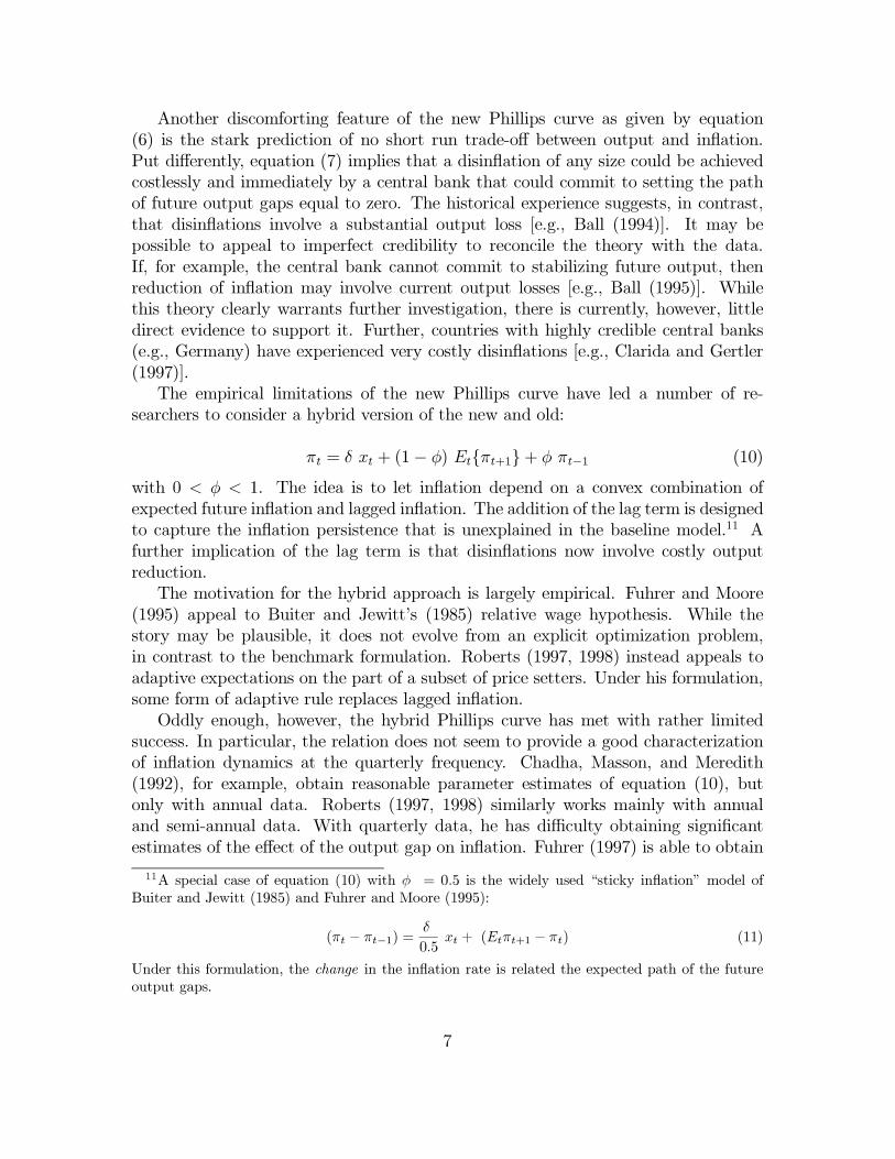
Reconciling the new Phillips curve with the data, has not proved to be a simple task.In particular, equation (6) implies that current change in inflation should dependnegatively on the lagged output gap. To see, lag equation (6) one period; and thenassume β � 1 to obtain
πt = −λκ xt−1 + πt−1 + εt (8)
where εt ≡ πt − Et−1πt. But estimating equation (8) with U.S. data, and using(quadratically) detrended log GDP as a measure of the output gap yields
πt = 0.081 xt−1 + πt−1 + εt (9)
i.e., the inflation rate depends positively on the lagged output gap rather than neg-atively: The estimated equation, unfortunately, resembles the old curve rather thanthe new!
The essential problem, as emphasized by Fuhrer and Moore (1995), is that thebenchmark new Phillips curve implies that inflation should lead the output gap overthe cycle, in the sense that a rise (decline) in current inflation should signal a subse-quent rise (decline) in the output gap. Yet, exactly the opposite pattern can be foundin the data. The top panel in Figure 1 presents the cross-correlation of the currentoutput gap (measured by detrended log GDP) with leads and lags of inflation.10 Asthe panel indicates clearly, the current output gap co-moves positively with futureinflation and negatively with lagged inflation. This lead of the output gap over infla-tion explains why the lagged output gap enters with a positive coefficient in equation(9), consistent with the old Phillips curve theory but in direct contradiction of thenew.
10The cross-correlations reported in figure 1 were computed on HP-detrended series over the period1960:1-1997:4. We provide a more extensive discussion of Figure 1 in the conclusion.
6
Another discomforting feature of the new Phillips curve as given by equation(6) is the stark prediction of no short run trade-off between output and inflation.Put differently, equation (7) implies that a disinflation of any size could be achievedcostlessly and immediately by a central bank that could commit to setting the pathof future output gaps equal to zero. The historical experience suggests, in contrast,that disinflations involve a substantial output loss [e.g., Ball (1994)]. It may bepossible to appeal to imperfect credibility to reconcile the theory with the data.If, for example, the central bank cannot commit to stabilizing future output, thenreduction of inflation may involve current output losses [e.g., Ball (1995)]. Whilethis theory clearly warrants further investigation, there is currently, however, littledirect evidence to support it. Further, countries with highly credible central banks(e.g., Germany) have experienced very costly disinflations [e.g., Clarida and Gertler(1997)].
The empirical limitations of the new Phillips curve have led a number of re-searchers to consider a hybrid version of the new and old:
πt = δ xt + (1− φ) Et{πt+1}+ φ πt−1 (10)
with 0 < φ < 1. The idea is to let inflation depend on a convex combination ofexpected future inflation and lagged inflation. The addition of the lag term is designedto capture the inflation persistence that is unexplained in the baseline model.11 Afurther implication of the lag term is that disinflations now involve costly outputreduction.
The motivation for the hybrid approach is largely empirical. Fuhrer and Moore(1995) appeal to Buiter and Jewitt’s (1985) relative wage hypothesis. While thestory may be plausible, it does not evolve from an explicit optimization problem,in contrast to the benchmark formulation. Roberts (1997, 1998) instead appeals toadaptive expectations on the part of a subset of price setters. Under his formulation,some form of adaptive rule replaces lagged inflation.
Oddly enough, however, the hybrid Phillips curve has met with rather limitedsuccess. In particular, the relation does not seem to provide a good characterizationof inflation dynamics at the quarterly frequency. Chadha, Masson, and Meredith(1992), for example, obtain reasonable parameter estimates of equation (10), butonly with annual data. Roberts (1997, 1998) similarly works mainly with annualand semi-annual data. With quarterly data, he has difficulty obtaining significantestimates of the effect of the output gap on inflation. Fuhrer (1997) is able to obtain
11A special case of equation (10) with φ = 0.5 is the widely used “sticky inflation” model ofBuiter and Jewitt (1985) and Fuhrer and Moore (1995):
(πt − πt−1) =δ
0.5xt + (Etπt+1 − πt) (11)
Under this formulation, the change in the inflation rate is related the expected path of the futureoutput gaps.
7

a significant output gap coefficient with quarterly data, but only when the model isheavily restricted. In this instance the estimated model is consistent with the oldPhillips curve: expected future inflation does not enter significantly in the inflationequation; lagged inflation enters with a coefficient near unity, as in the traditionalframework.
2.3 Shortcomings
There are, however, several problems with this approach that could possibly accountfor the empirical shortcomings. First, conventional measures of the output gap xtare likely to be ridden with error, primarily due to the unobservability of the naturalrate of output y∗t .
12 A typical approach (followed above) to measuring y∗t is to usea fitted deterministic trend. Alternatives are to use the Congressional Budget Office(CBO) estimate or instead use a measure of capacity utilization as the gap variable.It is widely agreed that all these approaches involve considerable measurement error.To the extent there is significant high frequency variation in y∗t (e.g., due to supplyshocks) mismeasurement could distort the estimation of an inflation equation like (6)or (10).13 Though, whether correcting for measurement error alone could reverse thelead-lag pattern between the output gap and inflation that is apparent from Figure1 is problematic in our view.
A more fundamental issue, we believe, is that even if the output gap were observ-able the conditions under which it corresponds to marginal cost may not be satisfied.Our analysis of the data suggests that movements in our measure of real marginalcost (described below) tend to lag movements in output, in direct contrast to theidentifying assumptions that imply a co-incident movement. This discrepancy, wewill argue, is one important reason why structural estimation of Phillips curves basedon the output gap have met with limited success, at best.
2.4 Our Approach
In light of the difficulties with using the output gap, we instead use in the empiricalanalysis below measures of real marginal cost, in a way consistent with the theory. Inother words, we estimate (3) instead of (6). Since real marginal cost is not directlyobservable, we use restrictions from theory to derive a measure based on observables.Conditional on our measure of real marginal cost, we can then obtain estimates of thestructural parameters in equation (3), including the frequency of price adjustment θ,
12This issue is currently of great practical importance in the U.S.: in recent years the measuredoutput gap is well above trend, but inflation is well below trend. It thus appears that mismeasure-ment of the true output gap is confounding the ability of traditional Phillips curves to explain thedata. See Lown and Rich (1997).
13For example, in the presence of nominal rigidities, supply shocks are likely to move detrendedoutput and the true output gap in opposite directions [Gali (1999)]. In addition, unobserved supplyshocks could potentially account for some of the explanatory power of lagged inflation.
8
the parameter that governs the degree of price stickiness (i.e., the average period aprice remains fixed.)
We also derive an econometric specification that permits us to assess the degreeto which the new Phillips curve can account for the inertia in inflation. In particular,we derive a “hybrid Phillips” curve that nests the new Phillips curve as a special case,but allows for a subset of firms use a backward looking rule of thumb to set prices.The advantage of proceeding this way is that the coefficients of our hybrid Phillipscurve will be functions of two key parameters: the frequency of price adjustmentand the fraction of backward looking price setters. Note that the latter parameterprovides a direct measure of the departure from a pure forward looking model neededto account for the persistence in inflation.
In the next section we present estimates of the new Phillips curve, and in thesubsequent one we present estimates of our hybrid Phillips curve.
3 New Estimates of the New Phillips Curve
We first describe our econometric specification of the new Phillips curve, along withour general estimation procedure. We then present both reduced form and structuralestimates of the model.
3.1 Econometric Specification
We begin by describing how we obtain a measure of real marginal cost. For simplicity,we restrict ourselves to the simplest measure of marginal cost available, one based onthe assumption of a Cobb-Douglas technology. Let At denote technology, Kt capital,and Nt labor. Then output Yt is given by
Yt = At Kαkt Nt
αn (12)
Real marginal cost is then given by the ratio of the wage rate to the marginalproduct of labor, i.e., MCt =
Wt
Pt1
∂Yt/∂Nt. Hence, given equation (12) we have:
MCt =St
αn(13)
where St ≡WtNt
PtYtis the labor income share (equivalently, real unit labor costs).14.
Letting lower case letters denote percent deviations from the steady state we have:
mct = st (14)
14Interestingly, Lown and Rich (1997) show that augmenting the growth of a traditional Phillipscurve with the growth rate of nominal unit labor costs greatly improves the fit. We also stress therole of unit labor costs, except that in our approach, (the log level) of real unit labor costs enters asthe relevant gap variable, as the theory suggests.
9
Combining equations (14) and (3) yields the inflation equation:
πt = λ st + β Et{πt+1} (15)
where the coefficient λ is given by
λ =(1− θ)(1− βθ)
θ(16)
Since under rational expectations the error in the forecast of πt+1 is uncorrelated withinformation dated t and earlier, it follows from equation (14) that
Et{(πt − λ st − β πt+1) zt} = 0 (17)
where zt is a vector of variables dated t and earlier (and, thus, orthogonal to theinflation surprise in period t+1). The orthogonality condition given by equation (17)then forms the basis for estimating the model via Generalized Method of Moments(GMM).
The data we use is quarterly for U.S. over the period 1960:1 to 1997:4. We use the(log) labor income share in the non-farm business sector for st. Our inflation measureis the percent change in the GDP deflator. We use the overall deflator rather than thenon-farm deflator for most of our analysis because we are interested evaluating howwell our model accounts for the movement in a standard broad measure of inflation.We show, however, that our results are robust to using the non-farm deflator. Finally,our instrument set includes four lags of inflation, the labor income share, output gap,the long-short interest rate spread, wage inflation, and commodity price inflation.
3.2 Reduced Form Evidence
We first report our estimate of equation (17). We refer to this evidence as “reducedform” since it contains an estimate of the overall slope coefficient on marginal cost,λ, but not of the structural parameter θ (the measure of price rigidity) that underliesλ (see equation 16). The resulting estimated equation is given byλ
πt = 0.023(0.012)
st+ 0.942(0.045)
Et{πt+1}
Overall, the estimated new Phillips curve is quite sensible. The slope coefficientλ on real marginal cost is positive and significant, as is consistent with the a prioritheory. The estimate of the coefficient on expected inflation, the subjective discountfactor β, is also reasonable, particularly after accounting for the sampling error im-plied by the estimated standard deviation.15 Thus, at first pass, it appears that thenew Phillips curve provides a reasonable description of inflation.
15In particular, the estimate of β is within two standard deviations of typical values for thisparameter that are used in the literature (e.g., 0.99).
10
To highlight the virtues of using real marginal cost as the relevant real sectordriving variable in the new Phillips curve, we reestimate equation (6), using detrendedlog GDP as a proxy for the output gap xt:
πt = − 0.016(0.005)
xt+ 0.988(0.030)
Et{πt+1}
The model clearly doesn’t work in this case: the coefficient associated with theoutput gap is negative and significant, which is at odds with the prediction of thetheory. This finding, of course, is completely consistent with our earlier result that,when the model is reversed and estimated in the form of the old Phillips curve, thecoefficient on the lagged output gap is positive (see equation (9)). Thus, it is theuse of real marginal cost over the output gap, and not the estimation strategy, thataccounts for the econometric success of the new Phillips curve.
3.3 Structural Estimates
We now redo the exercise in a way that allows us to obtain direct estimates of thestructural parameter θ. In particular, we substitute the relation for λ, equation (16),into equation (17) to obtain an econometric specification that is nonlinear in thestructural parameters θ and β.
One econometric issue we must confront is that, in small samples, nonlinear esti-mation using GMM is sometimes sensitive to the way the orthogonality conditions arenormalized. For this reason, we use two alternative specifications of the orthogonalityconditions as the basis for our GMM estimation procedure.16 The first specificationtakes the form
Et{(θ πt − (1− θ)(1− βθ) st − θβ πt+1) zt} = 0 (18)
while the second is given by:
Et{(πt − θ−1(1− θ)(1− βθ) st − β πt+1) zt} = 0 (19)
We estimate the structural parameters θ and β using a nonlinear instrumentalvariables estimator, with the set of instruments the same as is in the previous case.For robustness, we consider two alternatives to the benchmark case. In the firstalternative we restrict the estimate of the discount factor β to unity. In the second, weuse the non-farm GDP deflator as opposed to the overall deflator. Finally, we estimateeach specification using the two different normalizations, as given by equations (18)and (19).
The results are reported in Table 1. The first two columns give the estimatesof θ and β. The third then gives the implied estimate of λ, the reduced form slope
16Among the possible normalizations we have chosen the two which we view as most natural. Thefirst one appears to minimize the non-linearities, while the second normalizes the inflation coefficientto unity. See, e.g., Fuhrer, Moore, and Schuh (1995) for further discussion of the normalization issue.
11
coefficient on real marginal cost. In general, the structural estimates tell the sameoverall story as the reduce form estimates. The implied estimate of λ is always positiveand is highly significant in every case but one (restricted β, normalization (2)). Theestimate of β in the unrestricted case is somewhat low, but not unreasonably so, giventhe sampling uncertainty.
The estimate of the structural parameter θ is somewhat large and also somewhatsensitive to the normalization in the GMM estimation. Using method (1), we estimateθ to be around 0.83 with a small standard error, which implies that prices are fixed forbetween roughly five and six quarters on average. That period length is close to theaverage price duration found in survey evidence, though perhaps on the high side.17
Method (2) yields a slightly higher estimate of θ, around 0.88. Since λ is decreasingin θ (greater price rigidity implies that inflation is less sensitive to movements in realmarginal cost), the higher estimates of θ implies a lower estimate of λ for method (2).
For several reasons, however, our estimates of the degree of price rigidity are likelyto be upward biased. First, it is likely that the labor share does not provide an exactmeasure of real marginal cost. In this instance, the estimate of the slope coefficientλ is likely to be biased towards zero. This translates into upward bias of θ, given theinverse link between the two parameters. Second, the underlying theory that is usedto identify θ from estimates of λ, assumes a constant markup of price over marginalcost in the absence of prices rigidities. If the markup in the frictionless benchmarkmodel were countercyclical, as much recent theory has argued, the implied estimateof θ would be lower.18 With a countercyclical markup, desired price setting is lesssensitive to movements in marginal cost, which could help account for low overallsensitivity of inflation to the labor share.
The model also works well in the sense that we do not reject the overidentifyingrestrictions. Though we do not report the results here, the p-values for the nullhypothesis that the error term is uncorrelated with the instruments are all in therange of 0.9 or higher. This kind of test has low power, however, since it is notapplied against any specific alternative hypothesis. In the next section we develop amore refined test to measure how well the model accounts for inflation dynamics.
4 A New Hybrid Phillips Curve
We now explicitly address the issue of how well the new Phillips curve captures theapparent inertia in inflation. To do so, we extend the basic Calvo model to allowfor a subset of firms that use a backward looking rule of thumb to set prices. Ourformulation allows us to estimate the fraction of firms that lies in this subset. Bydoing so we obtain a measure of the residual inertia in inflation that the baseline new
17See Taylor (1998) for an overview of that evidence.18See, e.g., Kimball (1995) for an illustration of a countercycical desired markup in the context of
a sticky price model.
12
Phillips curve leaves unexplained.19
4.1 Theoretical Formulation
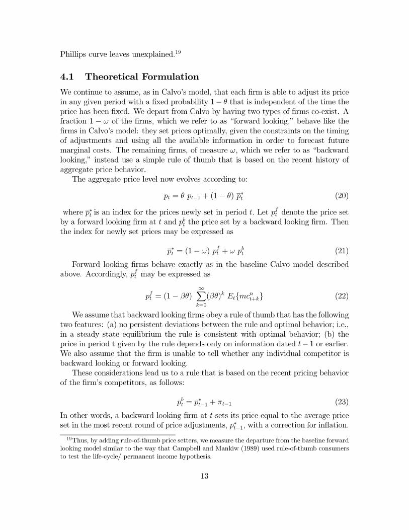
We continue to assume, as in Calvo’s model, that each firm is able to adjust its pricein any given period with a fixed probability 1− θ that is independent of the time theprice has been fixed. We depart from Calvo by having two types of firms co-exist. Afraction 1 − ω of the firms, which we refer to as “forward looking,” behave like thefirms in Calvo’s model: they set prices optimally, given the constraints on the timingof adjustments and using all the available information in order to forecast futuremarginal costs. The remaining firms, of measure ω, which we refer to as “backwardlooking,” instead use a simple rule of thumb that is based on the recent history ofaggregate price behavior.
The aggregate price level now evolves according to:
pt = θ pt−1 + (1− θ) p∗t (20)
where p∗t is an index for the prices newly set in period t. Let pft denote the price setby a forward looking firm at t and pbt the price set by a backward looking firm. Thenthe index for newly set prices may be expressed as
p∗t = (1− ω) pft + ω pbt (21)
Forward looking firms behave exactly as in the baseline Calvo model describedabove. Accordingly, pft may be expressed as
pft = (1− βθ)
∞∑k=0
(βθ)k Et{mcnt+k} (22)
We assume that backward looking firms obey a rule of thumb that has the followingtwo features: (a) no persistent deviations between the rule and optimal behavior; i.e.,in a steady state equilibrium the rule is consistent with optimal behavior; (b) theprice in period t given by the rule depends only on information dated t− 1 or earlier.We also assume that the firm is unable to tell whether any individual competitor isbackward looking or forward looking.
These considerations lead us to a rule that is based on the recent pricing behaviorof the firm’s competitors, as follows:
pbt = p∗t−1 + πt−1 (23)
In other words, a backward looking firm at t sets its price equal to the average priceset in the most recent round of price adjustments, p∗t−1, with a correction for inflation.
19Thus, by adding rule-of-thumb price setters, we measure the departure from the baseline forwardlooking model similar to the way that Campbell and Mankiw (1989) used rule-of-thumb consumersto test the life-cycle/ permanent income hypothesis.
13
Importantly, the correction is based on the lagged inflation rate, i.e., lagged inflationis used in a simple way to forecast current inflation.
Though admittedly ad hoc, the rule has several appealing features. First, as longas inflation is stationary, the rule converges to optimal behavior over time.20 Second,the rule implicitly incorporates information about the future in a useful way, sincethe price index p∗t−1 is partly determined by forward looking price setters. Thus,to the extent the percent difference between the forward and backward price is notlarge, the loss to a firm from rule of thumb behavior will be second order, for theusual arguments due to the envelope theorem. This is more likely to be the case ifbackward looking price setters are a relatively small fraction of the population.21
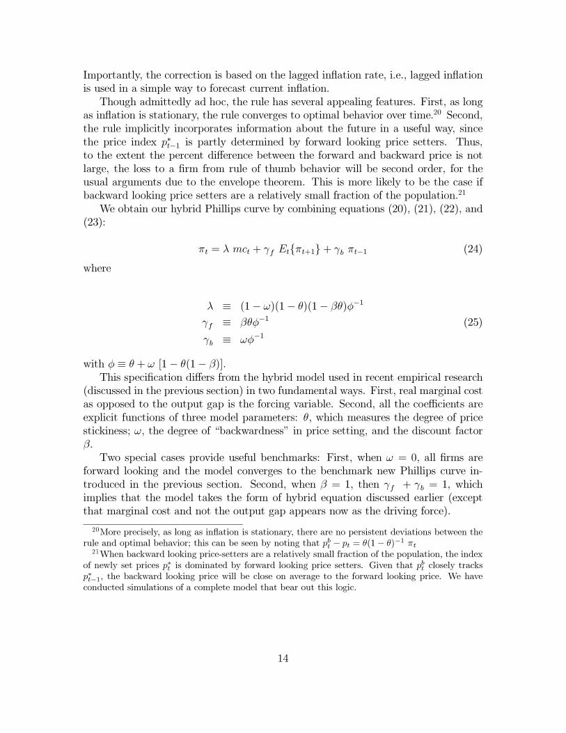
We obtain our hybrid Phillips curve by combining equations (20), (21), (22), and(23):
πt = λ mct + γf Et{πt+1}+ γb πt−1 (24)
where
λ ≡ (1− ω)(1− θ)(1− βθ)φ−1
γf ≡ βθφ−1 (25)
γb ≡ ωφ−1
with φ ≡ θ + ω [1− θ(1− β)].This specification differs from the hybrid model used in recent empirical research
(discussed in the previous section) in two fundamental ways. First, real marginal costas opposed to the output gap is the forcing variable. Second, all the coefficients areexplicit functions of three model parameters: θ, which measures the degree of pricestickiness; ω, the degree of “backwardness” in price setting, and the discount factorβ.
Two special cases provide useful benchmarks: First, when ω = 0, all firms areforward looking and the model converges to the benchmark new Phillips curve in-troduced in the previous section. Second, when β = 1, then γf + γb = 1, whichimplies that the model takes the form of hybrid equation discussed earlier (exceptthat marginal cost and not the output gap appears now as the driving force).
20More precisely, as long as inflation is stationary, there are no persistent deviations between therule and optimal behavior; this can be seen by noting that pb
t− pt = θ(1− θ)−1 πt
21When backward looking price-setters are a relatively small fraction of the population, the indexof newly set prices p∗t is dominated by forward looking price setters. Given that p
bt closely tracks
p∗t−1, the backward looking price will be close on average to the forward looking price. We haveconducted simulations of a complete model that bear out this logic.
14
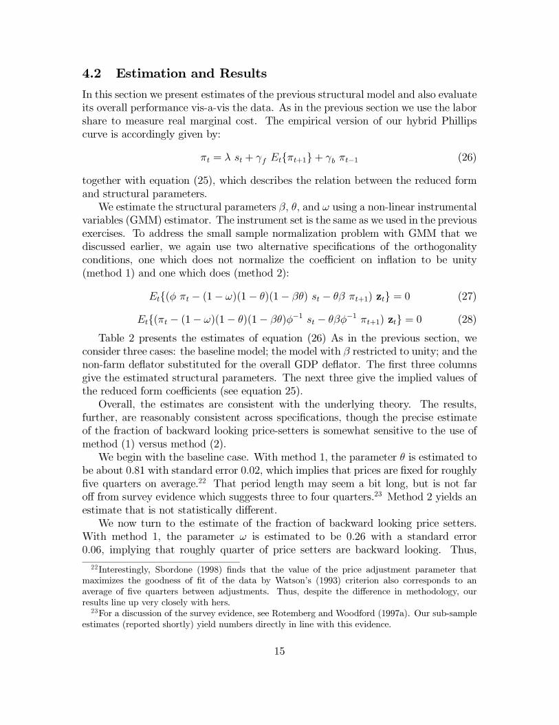
4.2 Estimation and Results
In this section we present estimates of the previous structural model and also evaluateits overall performance vis-a-vis the data. As in the previous section we use the laborshare to measure real marginal cost. The empirical version of our hybrid Phillipscurve is accordingly given by:
πt = λ st + γf Et{πt+1}+ γb πt−1 (26)
together with equation (25), which describes the relation between the reduced formand structural parameters.
We estimate the structural parameters β, θ, and ω using a non-linear instrumentalvariables (GMM) estimator. The instrument set is the same as we used in the previousexercises. To address the small sample normalization problem with GMM that wediscussed earlier, we again use two alternative specifications of the orthogonalityconditions, one which does not normalize the coefficient on inflation to be unity(method 1) and one which does (method 2):
Et{(φ πt − (1− ω)(1− θ)(1− βθ) st − θβ πt+1) zt} = 0 (27)
Et{(πt − (1− ω)(1− θ)(1− βθ)φ−1 st − θβφ−1 πt+1) zt} = 0 (28)
Table 2 presents the estimates of equation (26) As in the previous section, weconsider three cases: the baseline model; the model with β restricted to unity; and thenon-farm deflator substituted for the overall GDP deflator. The first three columnsgive the estimated structural parameters. The next three give the implied values ofthe reduced form coefficients (see equation 25).
Overall, the estimates are consistent with the underlying theory. The results,further, are reasonably consistent across specifications, though the precise estimateof the fraction of backward looking price-setters is somewhat sensitive to the use ofmethod (1) versus method (2).
We begin with the baseline case. With method 1, the parameter θ is estimated tobe about 0.81 with standard error 0.02, which implies that prices are fixed for roughlyfive quarters on average.22 That period length may seem a bit long, but is not faroff from survey evidence which suggests three to four quarters.23 Method 2 yields anestimate that is not statistically different.
We now turn to the estimate of the fraction of backward looking price setters.With method 1, the parameter ω is estimated to be 0.26 with a standard error0.06, implying that roughly quarter of price setters are backward looking. Thus,
22Interestingly, Sbordone (1998) finds that the value of the price adjustment parameter thatmaximizes the goodness of fit of the data by Watson’s (1993) criterion also corresponds to anaverage of five quarters between adjustments. Thus, despite the difference in methodology, ourresults line up very closely with hers.
23For a discussion of the survey evidence, see Rotemberg and Woodford (1997a). Our sub-sampleestimates (reported shortly) yield numbers directly in line with this evidence.
15

the pure forward looking model is rejected by the data. However, the quantitativeimportance of backward looking behavior for inflation dynamics is not large. Theimplied estimates for the reduced form coefficients on lagged versus expected futureinflation are 0.25 (for γb) and 0.68 (for γf ). Method 2 yields a higher estimate ofω, 0.49, implying that nearly half of price setters are backward looking. However,forward looking behavior remains predominant: The implied estimate of γf is 0.59versus 0.38 for γb.
Thus, while the results suggest some imprecision in the estimate of the degree ofbackwardness, the central conclusions do not change across methods (1) and (2): Inaccounting for inflation dynamics, forward looking behavior is more important thanbackward looking behavior. In either case the estimate of the coefficient on expectedfuture inflation in equation (26) lies well above the coefficient on lagged inflation.It is also true in either case that the estimates of the primitive parameters yield anestimate of the slope coefficient on the labor share λ that is positive and significant.24
Thus, we are able to identify (in a robust manner) a significant impact of marginalcosts on inflation.
It is also the case the model estimated using method (1) does a better job oftracking actual inflation the model based on method (2) estimates. (In section 4.4we make precise the sense in how we evaluate the ability of the model to track thedata.) To the extent that this provides a ground for preferring method (1), we canconclude that not only is forward looking behavior predominant but, given the smallestimate of the degree of backwardness, the pure forward looking model may do areasonably good job of describing the data.
The estimate of β is reasonably similar across the two methods, but somewhaton the low side at roughly 0.90. We thus next explore the implications of restrictingβ equal to unity, as implied in the standard hybrid case. Interestingly, there is littleimpact on the estimates of the other primitive parameters. Thus, restricting β to aplausible range does not affect the results in any significant way.
Finally, we consider the use of the non-farm deflator. Interestingly, there is nosignificant impact on the estimate of the degree of price rigidity. However, the es-timate of the degree of backwardness drops. Indeed, with method (1), the estimateof ω is only 0.07. Though somewhat larger with method 2, it is still just 0.239. Ineither case, backward looking behavior is not quantitatively important. Overall, thepure forward looking model may provide a reasonably good description of inflation,as measured by the non-farm deflator.
24We note that the link between inflation and marginal cost is related to Benabou’s (1992) findingusing retail trade data that inflation is inversely related to the markup (which he measured as theinverse of the labor share). He interpreted the findings as evidence that the markup may depend oninflation, whereas in our model, causation runs from marginal cost to inflation. Sorting out possiblesimultaneity is an interesting topic for future research. We note, however, that our model has theadditional implication that inflation should be related to a discounted stream of future marginalcosts, and we shortly demonstrate that this appears to be the case.
16

4.3 Robustness Analysis
We now consider two robustness exercises.25 The first allows extra lags of inflation toenter the right hand side of the equation for inflation. The second explores sub-samplestability.
We next add three additional lags of inflation to the baseline case (equation (26)).Here the idea is to explore whether our estimated importance of forward lookingbehavior may reflect not allowing for sufficient lagged dependence. Put differently,since we use four lags of inflation in our instrument set, we may be inadvertentlybiasing our “horse race” between expected future inflation and one quarter laggedinflation in favor of the former. The way to address this issue is to add the threeadditional lags of inflation to the right hand side, and then determine wether theyhave any predictive power for current inflation, πt, beyond the signalling power theyhave for expected future inflation, Et{πt+1}.
Table 3 report the results. The parameter ψ denotes the sum of the coefficientson the three additional inflation lags. Since the estimates do not change much acrossmethod (1) and (2), we only report results for the former case. The overall effect ofthe additional lags is quite small, especially when the GDP deflator is used as themeasure of inflation. The estimate of ψ is only 0.09 in the baseline case, and notsignificantly different from zero when β is restricted to unity. When the non-farmdeflator is used the estimate of ψ rise to 0.21 with a standard error of 0.06. However,in this instance the first lag of inflation is not significantly different, so that theoverall effect of lagged inflation is minimal. Thus, even though a total of four lags ofinflation enters the right hand side, forward looking behavior still predominates. Itthus appears that we account for inflation inertia with minimal reliance on arbitrarylags.
Finally, we consider sub-sample stability. Table 4 reports estimates over the in-tervals 60:1-79:4, 70:1-89:4, and 80:1-97:4. Again, since the conclusions we draware unaffected by the normalization used, we restrict attention to method (1).
Overall, the broad picture remains unchanged. Marginal costs have a significantimpact on short run inflation dynamics of roughly the same quantitative magnitudesas suggested by the full sample estimates. Forward looking behavior is always im-portant. For the GDP deflator, in the first two sub-periods, the estimate of ω isclose to the full sample estimate; i.e. roughly 0.25. Interestingly, though, in the lastsub-period the estimate of ω drops in half to about 0.12. The pattern is the oppo-site for the non-farm deflator: estimates of ω near zero for the first two sub-samples(which correspond to the full-sample estimates), but rising slightly to 0.22 in the lastsub-sample.
Another interesting result with the GDP deflator is that the estimate of θ for the
25In an earlier version of the paper we also allowed for increasing returns (in the form of overheadlabor) in constructing the measure of marginal cost. Since this modification does not affect theresults, we do not report the exercise here.
17
first two sub-samples drops from the full sample estimate of 0.8 to the range 0.75−0.77. The important implication is that pre-1990, the estimated average duration aprice is fixed is around four quarters, which is directly in line with the survey evidence.For the last sample, 1980:1 -1997:4, the estimate of θ rises to roughly 0.85, implyingduration of six quarters. The longer duration might reflect the fact that inflation waslower over the last sub-sample. As a consequence, the average length between priceadjustments may have increased (as, for example, a model of state-dependent pricingmight imply.)
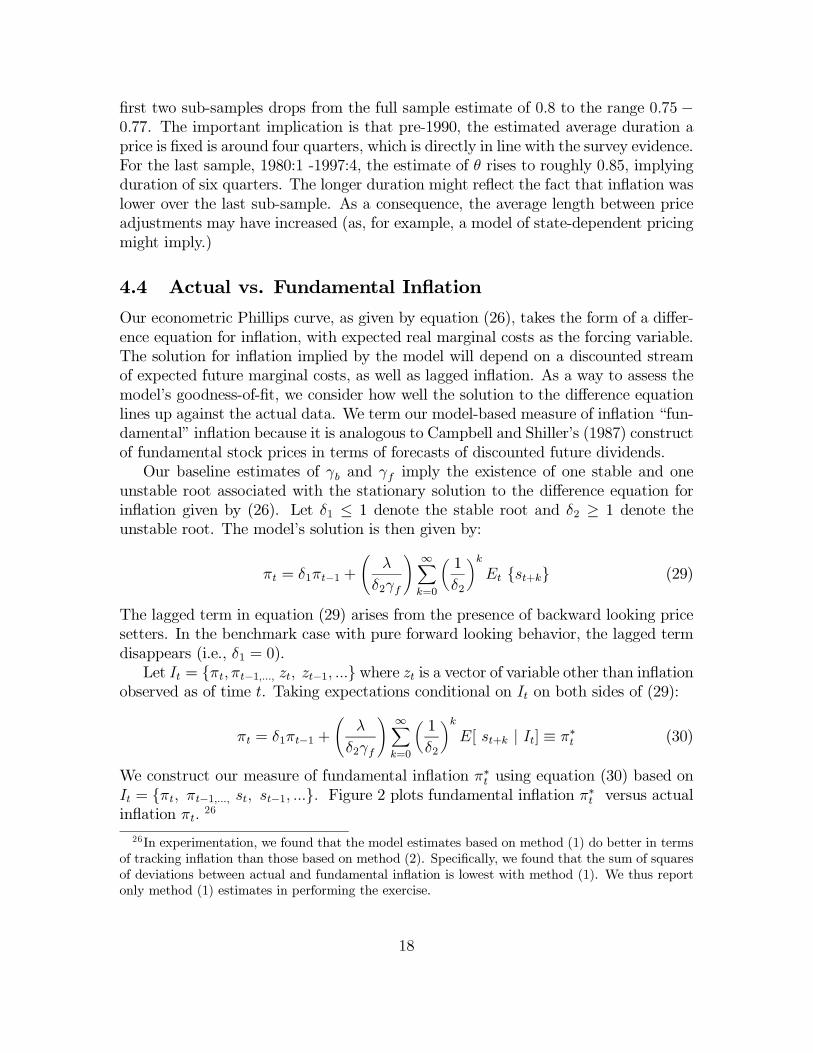
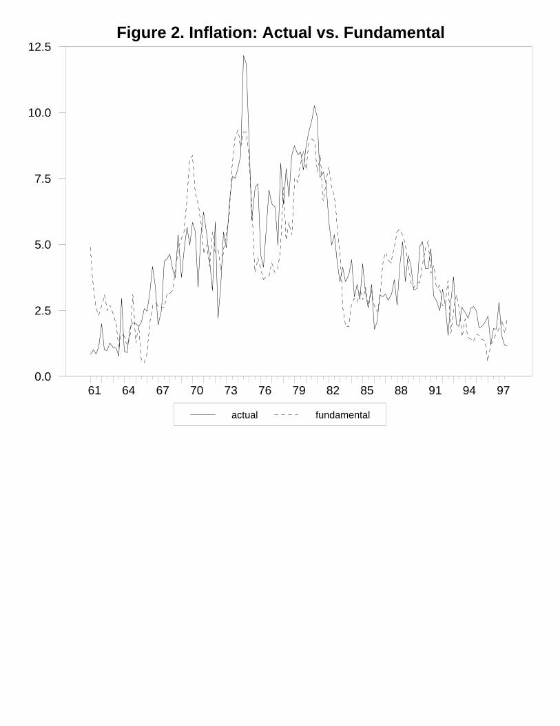
4.4 Actual vs. Fundamental Inflation
Our econometric Phillips curve, as given by equation (26), takes the form of a differ-ence equation for inflation, with expected real marginal costs as the forcing variable.The solution for inflation implied by the model will depend on a discounted streamof expected future marginal costs, as well as lagged inflation. As a way to assess themodel’s goodness-of-fit, we consider how well the solution to the difference equationlines up against the actual data. We term our model-based measure of inflation “fun-damental” inflation because it is analogous to Campbell and Shiller’s (1987) constructof fundamental stock prices in terms of forecasts of discounted future dividends.
Our baseline estimates of γb and γf imply the existence of one stable and oneunstable root associated with the stationary solution to the difference equation forinflation given by (26). Let δ1 ≤ 1 denote the stable root and δ2 ≥ 1 denote theunstable root. The model’s solution is then given by:
πt = δ1πt−1 +
(λ
δ2γf
)∞∑k=0
(1
δ2
)kEt {st+k} (29)
The lagged term in equation (29) arises from the presence of backward looking pricesetters. In the benchmark case with pure forward looking behavior, the lagged termdisappears (i.e., δ1 = 0).
Let It = {πt, πt−1,..., zt, zt−1, ...} where zt is a vector of variable other than inflationobserved as of time t. Taking expectations conditional on It on both sides of (29):
πt = δ1πt−1 +
(λ
δ2γf
)∞∑k=0
(1
δ2
)kE[ st+k | It] ≡ π∗t (30)
We construct our measure of fundamental inflation π∗t using equation (30) based onIt = {πt, πt−1,..., st, st−1, ...}. Figure 2 plots fundamental inflation π∗t versus actualinflation πt.
26
26In experimentation, we found that the model estimates based on method (1) do better in termsof tracking inflation than those based on method (2). Specifically, we found that the sum of squaresof deviations between actual and fundamental inflation is lowest with method (1). We thus reportonly method (1) estimates in performing the exercise.
18

Overall fundamental inflation tracks the behavior of actual inflation very well.27
It is particularly interesting to observe that it does a good job of explaining the recentbehavior of inflation. During the past several years, of course, inflation has been belowtrend. Output growth has been above trend, on the other hand, making standardmeasures of the output gap highly positive. As a consequence, traditional Phillipscurve equations have been overpredicting recent inflation.28 However, because, realunit labor costs have been quite moderate recently despite rapid output growth, ourmodel of fundamental inflation is close to target.
5 Conclusions
Our results suggest that, conditional on the path of real marginal costs, the baselinenew Phillips curve with forward looking behavior may provide a reasonably gooddescription of inflation dynamics. When tested explicitly against an alternative thatallows for a fraction of price setters to be backward looking, the structural estimatessuggest that this fraction, while statistically significant, is not quantitatively impor-tant. One qualification, however, is that there is some imprecision in our estimatesof the importance of backward looking behavior. Yet, across all specifications for-ward looking behavior remains dominant. In the estimated hybrid Phillips curve, theweight on inflation lagged one quarter is generally small. Further, additional lags ofinflation beyond one quarter do not appear to matter much at all. Taken as a whole,accordingly, the results suggest that it is worth searching for explanations of inflationinertia beyond the traditional ones that rely heavily on arbitrary lags.
One important avenue to investigate, we think, involves the cyclical behavior ofreal marginal cost. Figure 1 presents sets of cross-correlations that help frame theissue. The data are quarterly from 1960:1-1997:4 and HP-detrended. The top panel,discussed earlier, displays the cross-correlation of inflation (the percent change inthe GDP deflator) with the output gap (i.e., detrended log GDP). The middle onecompares the output gap and the labor income share (our measure of real marginalcosts), while the last one looks at the labor share and inflation.
Among other things, the figure makes clear why real unit labor costs outperformsthe output gap in the estimation of the new Phillips curve. As the top panel indicates,the output gap leads inflation, rather than vice-versa, in direct contradiction of thetheory (see equation (7)). In contrast, as the third panel indicates, real unit laborcosts exhibit a strong contemporaneous correlation with inflation. Further, laggedinflation is positively correlated with current unit labor costs, consistent with the
27Sbordone (1998) similarly finds that inflation is well explained by a discounted stream of futurereal marginal costs, though using a quite different methodology to parametrize the model.
28An exception is Lown and Rich (1997). Because they augment a traditional Phillips curvewith the growth in nominal unit labor costs, their equation fares much better than the standardformulation. Though the way unit labor costs enters our formulation is quite different, it is similarlythe sluggish behavior of unit labor costs that helps the model explain recent inflation.
19

theory. Thus, (with the benefit of this hindsight), it is perhaps not surprising whyreal unit labor costs enters the structural inflation equation significantly and with theright sign. The middle panel completes the picture: the labor income share lags theoutput gap in much the same way as does inflation. The lag in the response of realunit labor costs explains why the output gap performs poorly in estimates of the newPhillips curve.
It is also true that the sluggish behavior of real marginal cost might help accountfor the slow response of inflation to output and thus (possibly) why disinflationsmay entail costly output reductions.29 For this reason, modifying existing theories toaccount for the rigidities in marginal costs suggested by Figure 1 could offer importantinsights for inflation dynamics.30 Given the link between unit labor costs andmarginalcosts, a candidate source for the necessary friction is wage rigidity. Indeed, a likelyreason for the strong counterfactual contemporaneous positive correlation betweenoutput and real marginal cost in the standard sticky price framework is the absence ofany type of labor market frictions [see, e.g., the discussion in Christiano, Eichenbaumand Evans (1997)]. At this stage, one cannot rule out whether it is nominal or realwage rigidities that can provide the answer. Both seem worth exploring.
29Interestingly, Blanchard and Muet (1992) find that disinflations in France have been associatedwith declines in real unit labor costs. In this respect it seems worth exploring data from othercountries.
30The existing literature on business cycle models that features sticky prices has long emphasizedthe need to incorporate real rigidities (see, e.g., Blanchard and Fischer (1989) and Ball and Romer(1990)). Typically, however, the discussion is in terms of trying to explain a large response of outputto monetary policy: Real rigidities help flatten the short run marginal cost curve. However, it isalso the case, as we have been arguing, that real rigidities may be needed to account for inflationdynamics, and in particular the sluggish response of inflation to movements in output.
20
REFERENCES
Ball, Laurence (1994): “What Determines the Sacrifice Ratio ?,” in G. Mankiw,ed., Monetary Policy, Chicago University Press.
Ball, Laurence (1995), “Disinflation with Imperfect Credibility,” Journal of Mon-etary Economics 35, 5-24.
Ball, Laurence and David Romer (1990), “Real Rigidities and the Non-Neutralityof Money,” Review of Economic Studies, 183-204.
Blanchard, Olivier and Pierre Alain Muet (1992), “Competitiveness Through Dis-inflation: An Assessment of the French Macro-Strategy,” mimeo, M.I.T.
Blanchard, Olivier and Stanley Fischer (1989), Lectures on Macroeconomics,M.I.T.Press.
Benabou, Roland, (1992), “Inflation and Markups: Theories and Evidence fromthe Retail Trade Sector, European Economic Review, 36, 566-574.
Bernanke, Ben S., Mark Gertler, and Simon Gilchrist, (1998), “The Financial Ac-celerator in a Quantitative Business Cycle Framework,” in the Handbook of Macro-economics, John Taylor and Michael Woodford eds.
Buiter Willem and Ian Jewitt, “Staggered Wage Setting with Real Wage Relativ-ities: Variations on a Theme of Taylor,” in Macroeconomic Theory and StabilizationPolicy (University of Michigan Press, Ann Arbor), 183-199.
Calvo, Guillermo A. (1983): “Staggered Prices in a Utility Maximizing Frame-work,” Journal of Monetary Economics, 12, 383-398.
Campbell, John Y. and N. Gregory Mankiw (1989), “Consumption, Income andInterest Rates: Re-interpreting the Times Series Evidence,” NBER MacroeconomicsAnnual, edited by Olivier Blanchard and Stanley Fischer (M.I.T. Press).
Campbell, John Y. and Robert Shiller (1987), “Cointegration and Tests of thePresent Value Relation,” Journal of Political Economy 95, 1062-1088.
Chadha, Bankim, Paul R. Masson and Guy Meredith (1992), “Models of Inflationand the Costs of Disinflation,” IMF Staff Papers, vol.39, no. 2, 395-431.
Chari, V.V., Patrick Kehoe and Ellen McGratten, (1996), “Sticky Price Models ofthe Business Cycle: The Persistence Problem,” manuscript, University of Minnesota.
Christiano, Lawrence J., Martin Eichenbaum and Charles Evans (1997), “StickyPrice and Limited Participation Models: A Comparison,” European Economic Re-view, 41, 1201-1249.
Clarida, Richard and Mark Gertler(1997), “How the Bundesbank Conducts Mon-etary Policy,” in Reducing Inflation: Motivation and Strategies, Christina and DavidRomer editors.
Clarida, Richard, Jordi Gali, and Mark Gertler, (1997a), “Monetary Policy Rulesand Macroeconomic Stability: Evidence and Some Theory,” Quarterly Journal ofEconomics, forthcoming.
Clarida, Richard, Jordi Gali, andMark Gertler (1997b): “The Science of MonetaryPolicy: A New Keynesian Perspective,” Journal of Economic Literature, forthcoming.
21

Erceg, Christopher J., Dale W. Henderson and Andrew Levin (1998), “Output-Gap and Price Inflation Volatilities: Reaffirming Tradeoffs in an Optimizing Model,”mimeo, Federal Reserve Board.
Fischer, Stanley, (1997): “Long Term Contracts, Rational Expectations, and theOptimal Money Supply Rule,” Journal of Political Economy 85, 163-190.
Fuhrer, Jeffrey C., and George R. Moore (1995): “Inflation Persistence”,QuarterlyJournal of Economics, No. 440, February, pp 127-159.
Fuhrer, Jeffrey C. (1997): “The (Un)Importance of Forward-Looking Behavior inPrice Specifications,” Journal of Money, Credit, and Banking 29, no. 3, 338-350.
Fuhrer, Jeffrey C., Geoffrey Moore, and Scott Schuh (1995): “Estimating theLinear-Quadratic Inventory: Maximum Likelihood versus Generalized Method of Mo-ments,” Journal of Monetary Economics 35, 115-157.
Galí, Jordi (1999): “Technology, Employment, and the Business Cycle: Do Tech-nology Shocks Explain Aggregate Fluctuations?,” American Economic Review, March
Ghezzi, Piero, (1997), “Backward Looking Indexation, Credibility and InflationPersistence,” John Hopkins University, mimeo.
Goodfriend, Marvin, and Robert King (1997): “The New Neoclassical Synthesisand the Role of Monetary Policy” NBER Macroeconomics Annual, forthcoming.
Gordon, Robert J.(1996), “Time-Varying NAIRU and its Implications for Eco-nomic Policy, NBER Working Paper No. 5735.
Jeanne, Olivier, (1998), “Generating Real Persistent Effects of Monetary Shocks:How Much Nominal Rigidity Do We Really Need?” European Economic Review no.6, 1009-1032.
Kiley, Michael T.(1997), “Staggered Price Setting and Real Rigidities,” FederalReserve Board FEDS working paper no. 1997-46.
Kimball, Miles S. (1995): “The Quantitative analytics of the Basic NeomonetaristModel,” Journal of Money, Credit, and Banking, vol. 27, no. 4, 1241-1278.
King, Robert G., and Alexander L. Wolman, (1996): “Inflation Targeting in a St.Louis Model of the 21st Century” NBER Working Paper No. 5507.
King, Robert G. and Alexander L. Wolman, (1998): “What Should The MonetaryAuthority Do When Prices Are Sticky?” forthcoming in Monetary Policy Rules, J.Taylor, ed, The University of Chicago Press.
King Robert G. and Mark Watson (1994), “The Post-War U.S. Phillips Curve: ARevisionist Econometric History,” Carnegie-Rochester Conference on Public Policy,157-219.
Lown Cara S. and Robert W. Rich (1997), “Is There An Inflation Puzzle,” FederalReserve Bank of New York Quarterly Review, 51-69.
McCallum, Bennett T., and Edward Nelson (1998): “Performance of OperationalPolicy Rules in an Estimated Semi-Classical Structural Model,” forthcoming inMon-etary Policy Rules, J. Taylor, ed, The University of Chicago Press.
Roberts, John M. (1997): “Is Inflation Sticky? ”, Journal of Monetary Economics,No. 39, pp 173-196.
22
Roberts, John M. (1998): “Inflation Expectations and the Transmission of Mon-etary Policy,” mimeo, Federal Reserve Board.
Rotemberg, Julio, andMichaelWoodford (1997a): “AnOptimization-Based Econo-metric Framework for the Evolution of Monetary Policy,” mimeo
Rotemberg, Julio and Michael Woodford (1997b): “Interest Rate Rules in a Esti-mated Sticky Price Model,” mimeo, Princeton University.
Sbordone, Argia, M., “Prices and Unit Labor Costs: Testing Models of Pricing,”mimeo, Princeton University.
Svensson, Lars E. O., (1997a), “Inflation Forecast Targeting: Implementing andMonitoring Inflation Targets”, European Economic Review 41, June, pp. 1111-47.
Svensson, Lars E. O., (1997b), “Inflation Targeting: Some Extensions”, NBERWorking Paper No. 5962, March.
Taylor, John B. (1980): “Aggregate Dynamics and Staggered Contracts,” Journalof Political Economy, 88, 1-23.
Watson, Mark, (1993). “Measures of Fit For Calibrated Models,” Journal ofPolitical Economy, 101-141.
Woodford, Michael (1996): “Control of the Public Debt: A Requirement for PriceStability?”, NBER Working Paper No. 5684, July .
Yun, Tack (1996): “Nominal Price Rigidity, Money Supply Endogeneity, andBusiness Cycles”, Journal of Monetary Economics, No. 37, 1996, pp 345-370.
23
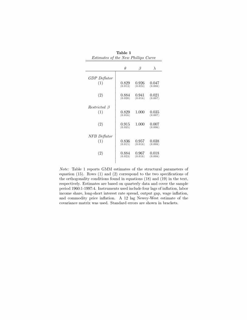
Table 1
Estimates of the New Phillips Curve
θ β λ
GDP Deflator
(1) 0.829(0.013)
0.926(0.024)
0.047(0.008)
(2) 0.884(0.020)
0.941(0.018)
0.021(0.007)
Restricted β
(1) 0.829(0.016)
1.000 0.035(0.007)
(2) 0.915(0.035)
1.000 0.007(0.006)
NFB Deflator
(1) 0.836(0.015)
0.957(0.018)
0.038(0.008)
(2) 0.884(0.023)
0.967(0.016)
0.018(0.008)
Note: Table 1 reports GMM estimates of the structural parameters ofequation (15). Rows (1) and (2) correspond to the two specifications ofthe orthogonality conditions found in equations (18) and (19) in the text,respectively. Estimates are based on quarterly data and cover the sampleperiod 1960:1-1997:4. Instruments used include four lags of inflation, laborincome share, long-short interest rate spread, output gap, wage inflation,and commodity price inflation. A 12 lag Newey-West estimate of thecovariance matrix was used. Standard errors are shown in brackets.
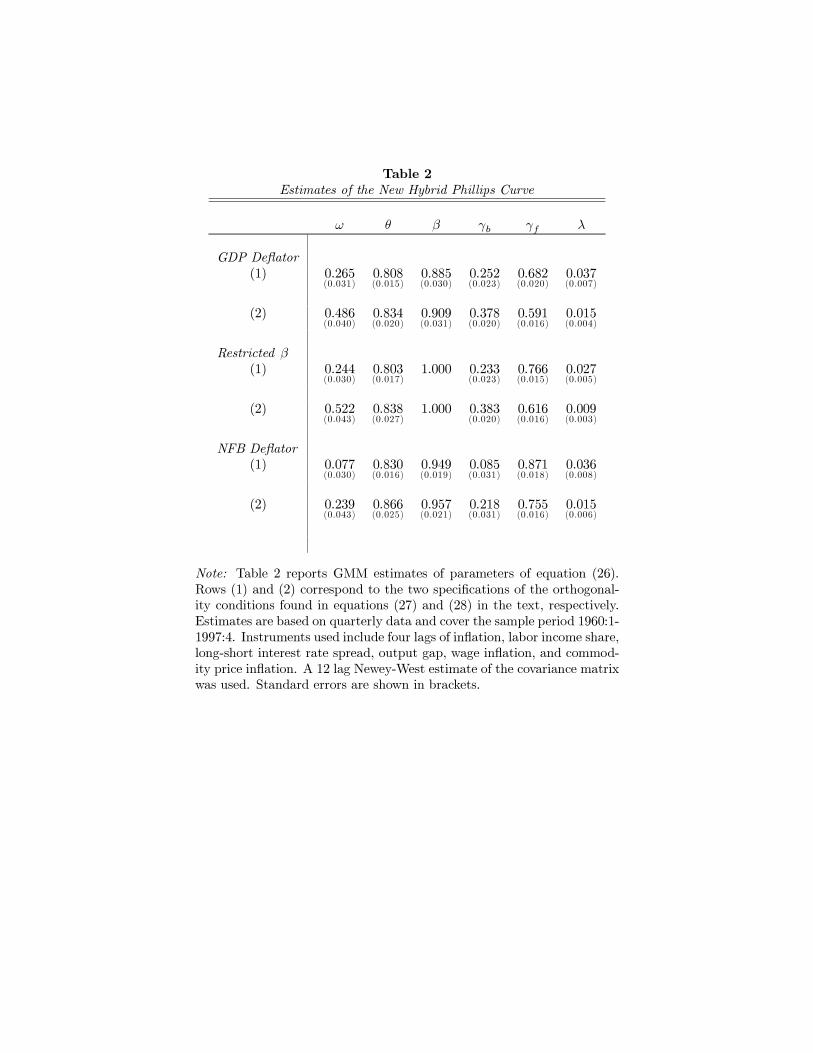
Table 2
Estimates of the New Hybrid Phillips Curve
ω θ β γb γf λ
GDP Deflator
(1) 0.265(0.031)
0.808(0.015)
0.885(0.030)
0.252(0.023)
0.682(0.020)
0.037(0.007)
(2) 0.486(0.040)
0.834(0.020)
0.909(0.031)
0.378(0.020)
0.591(0.016)
0.015(0.004)
Restricted β
(1) 0.244(0.030)
0.803(0.017)
1.000 0.233(0.023)
0.766(0.015)
0.027(0.005)
(2) 0.522(0.043)
0.838(0.027)
1.000 0.383(0.020)
0.616(0.016)
0.009(0.003)
NFB Deflator
(1) 0.077(0.030)
0.830(0.016)
0.949(0.019)
0.085(0.031)
0.871(0.018)
0.036(0.008)
(2) 0.239(0.043)
0.866(0.025)
0.957(0.021)
0.218(0.031)
0.755(0.016)
0.015(0.006)
Note: Table 2 reports GMM estimates of parameters of equation (26).Rows (1) and (2) correspond to the two specifications of the orthogonal-ity conditions found in equations (27) and (28) in the text, respectively.Estimates are based on quarterly data and cover the sample period 1960:1-1997:4. Instruments used include four lags of inflation, labor income share,long-short interest rate spread, output gap, wage inflation, and commod-ity price inflation. A 12 lag Newey-West estimate of the covariance matrixwas used. Standard errors are shown in brackets.
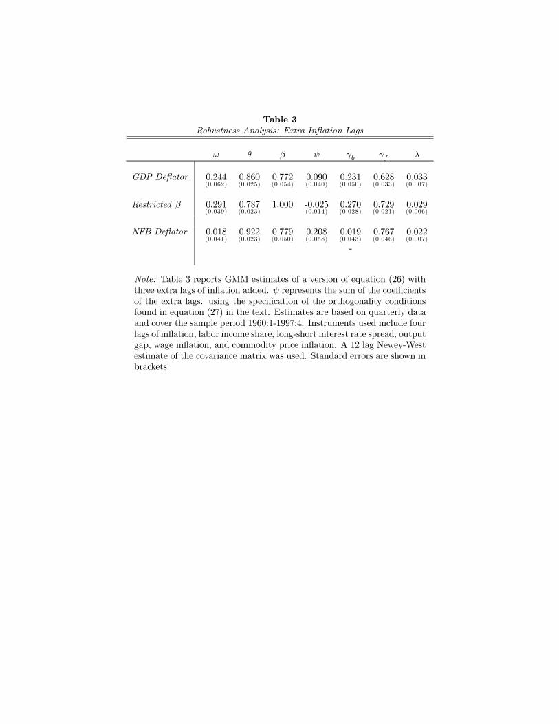
Table 3
Robustness Analysis: Extra Inflation Lags
ω θ β ψ γb γf λ
GDP Deflator 0.244(0.062)
0.860(0.025)
0.772(0.054)
0.090(0.040)
0.231(0.050)
0.628(0.033)
0.033(0.007)
Restricted β 0.291(0.039)
0.787(0.023)
1.000 -0.025(0.014)
0.270(0.028)
0.729(0.021)
0.029(0.006)
NFB Deflator 0.018(0.041)
0.922(0.023)
0.779(0.050)
0.208(0.058)
0.019(0.043)
0.767(0.046)
0.022(0.007)
-
Note: Table 3 reports GMM estimates of a version of equation (26) withthree extra lags of inflation added. ψ represents the sum of the coefficientsof the extra lags. using the specification of the orthogonality conditionsfound in equation (27) in the text. Estimates are based on quarterly dataand cover the sample period 1960:1-1997:4. Instruments used include fourlags of inflation, labor income share, long-short interest rate spread, outputgap, wage inflation, and commodity price inflation. A 12 lag Newey-Westestimate of the covariance matrix was used. Standard errors are shown inbrackets.
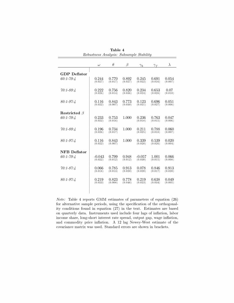
Table 4
Robustness Analysis: Subsample Stability
ω θ β γb γf λ
GDP Deflator
60:1-79:4 0.244(0.027)
0.770(0.017)
0.892(0.027)
0.245(0.022)
0.691(0.016)
0.054(0.007)
70:1-89:4 0.222(0.026)
0.756(0.014)
0.820(0.036)
0.234(0.024)
0.653(0.028)
0.07(0.010)
80:1-97:4 0.116(0.022)
0.843(0.007)
0.773(0.030)
0.123(0.021)
0.696(0.027)
0.051(0.006)
Restricted β
60:1-79:4 0.233(0.022)
0.753(0.016)
1.000 0.236(0.018)
0.763(0.015)
0.047(0.006)
70:1-89:4 0.196(0.026)
0.734(0.017)
1.000 0.211(0.025)
0.788(0.018)
0.060(0.007)
80:1-97:4 0.116(0.022)
0.843(0.007)
1.000 0.339(0.020)
0.539(0.026)
0.020(0.004)
NFB Deflator
60:1-79:4 -0.043(0.022)
0.799(0.012)
0.948(0.012)
-0.057(0.030)
1.001(0.015)
0.066(0.008)
70:1-87:4 0.066(0.018)
0.785(0.013)
0.913(0.020)
0.078(0.020)
0.846(0.017)
0.913(0.020)
80:1-97:4 0.219(0.023)
0.823(0.008)
0.778(0.046)
0.219(0.023)
0.638(0.034)
0.049(0.005)
Note: Table 4 reports GMM estimates of parameters of equation (26)for alternative sample periods, using the specification of the orthogonal-ity conditions found in equation (27) in the text. Estimates are basedon quarterly data. Instruments used include four lags of inflation, laborincome share, long-short interest rate spread, output gap, wage inflation,and commodity price inflation. A 12 lag Newey-West estimate of thecovariance matrix was used. Standard errors are shown in brackets.
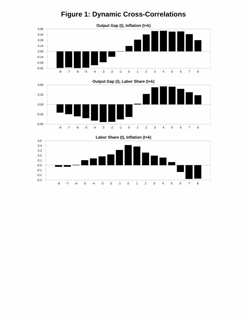
Figure 1: Dynamic Cross-Correlations
Output Gap (t), Inflation (t+k)
-8 -7 -6 -5 -4 -3 -2 -1 0 1 2 3 4 5 6 7 8-0.42
-0.28
-0.14
0.00
0.14
0.28
0.42
0.56
Output Gap (t), Labor Share (t+k)
-8 -7 -6 -5 -4 -3 -2 -1 0 1 2 3 4 5 6 7 8-0.50
-0.25
0.00
0.25
0.50
Labor Share (t), Inflation (t+k)
-8 -7 -6 -5 -4 -3 -2 -1 0 1 2 3 4 5 6 7 8-0.3
-0.2
-0.1
-0.0
0.1
0.2
0.3
0.4
0.5
actual fundamental
Figure 2. Inflation: Actual vs. Fundamental
61 64 67 70 73 76 79 82 85 88 91 94 970.0
2.5
5.0
7.5
10.0
12.5