NBER WORKING PAPER SERIES

IMPERFECT KNOWLEDGE, INFLATION EXPECTATIONS,AND MONETARY POLICY

Athanasios OrphanidesJohn C. Williams

Working Paper 9884http://www.nber.org/papers/w9884

NATIONAL BUREAU OF ECONOMIC RESEARCH1050 Massachusetts Avenue

Cambridge, MA 02138July 2003

Presented at the Inflation Targeting conference, January 23-25, 2003, organized by Michael Woodford. Wewould like to thank Roger Craine, George Evans, Stan Fischer, Mark Gertler, John Leahy, Bill Poole, TomSargent, Lars Svensson, and participants at meetings of the Econometric Society, the Society ofComputational Economics, the University of Cyprus, the Federal Reserve Banks of San Francisco andRichmond, the NBER Monetary Economics Program, and the NBER Universities Research Conference onMacroeconomic Policy in a Dynamic Uncertain Economy for useful comments and discussions on earlierdrafts. We thank Adam Litwin for research assistance and Judith Goff for editorial assistance. The opinionsexpressed are those of the authors and do not necessarily reflect views of the Board of Governors of theFederal Reserve System or the Federal Reserve Bank of San Francisco. The views expressed herein are thoseof the authors and not necessarily those of the National Bureau of Economic Research.

©2003 by Athanasios Orphanides and John C. Williams. All rights reserved. Short sections of text, not toexceed two paragraphs, may be quoted without explicit permission provided that full credit, including ©notice, is given to the source.

Imperfect Knowledge, Inflation Expectations, and Monetary PolicyAthanasios Orphanides and John C. WilliamsNBER Working Paper No. 9884July 2003JEL No. E52

ABSTRACT

This paper investigates the role that imperfect knowledge about the structure of the economy plays

in the formation of expectations, macroeconomic dynamics, and the efficient formulation of

monetary policy. Economic agents rely on an adaptive learning technology to form expectations and

to update continuously their beliefs regarding the dynamic structure of the economy based on

incoming data. The process of perpetual learning introduces an additional layer of dynamic

interaction between monetary policy and economic outcomes. We find that policies that would be

efficient under rational expectations can perform poorly when knowledge is imperfect. In particular,

policies that fail to maintain tight control over inflation are prone to episodes in which the public’s

expectations of inflation become uncoupled from the policy objective and stagflation results, in a

pattern similar to that experienced in the United States during the 1970s. Our results highlight the

value of effective communication of a central bank’s inflation objective and of continued vigilance

against inflation in anchoring inflation expectations and fostering macroeconomic stability.

Athanasios Orphanides John C. WilliamsFederal Reserve Board Federal Reserve Bank of San FranciscoWashington, DC 20551 101 Market Streetathanasios.orphanides@frb.gov San Francisco, CA 94105

john.c.williams@sf.frb.org

1 Introduction

Rational expectations provides an elegant and powerful framework that has come to dom-

inate thinking about the dynamic structure of the economy and econometric policy evalu-

ation over the past 30 years. This success has spurred further examination into the strong

information assumptions implicit in many of its applications. Thomas Sargent (1993) con-

cludes that “rational expectations models impute much more knowledge to the agents within

the model ... than is possessed by an econometrician, who faces estimation and inference

problems that the agents in the model have somehow solved” (p. 3, emphasis in original).1

Researchers have proposed refinements to rational expectations that respect the principle

that agents use information efficiently in forming expectations, but nonetheless recognize

the limits to and costs of information-processing and cognitive constraints that influence the

expectations-formation process (Sargent 1999, Evans and Honkapohja 2001, Sims 2003).

In this study, we allow for a form of imperfect knowledge in which economic agents

rely on an adaptive learning technology to form expectations. This form of learning rep-

resents a relatively modest deviation from rational expectations that nests it as a limiting

case. We show that the resulting process of perpetual learning introduces an additional

layer of interaction between monetary policy and economic outcomes that has important

implications for macroeconomic dynamics and for monetary policy design. As we illustrate,

monetary policies that would be efficient under rational expectations can perform poorly

when knowledge is imperfect. In particular, with imperfect knowledge, policies that fail to

maintain tight control over inflation are prone to episodes in which the public’s expectations

of inflation become uncoupled from the policy objective. The presence of this imperfection

makes stabilization policy more difficult than would appear under rational expectations and1Missing from such models, as Benjamin Friedman (1979) points out, “is a clear outline of the way in

which economic agents derive the knowledge which they then use to formulate expectations.” To be sure,this does not constitute a criticism of the traditional use of the concept of “rationality” as reflecting theoptimal use of information in the formation of expectations, taking into account an agent’s objectives andresource constraints. The difficulty is that in Muth’s (1961) original formulation, rational expectations arenot optimizing in that sense. Thus, the issue is not that the “rational expectations” concept reflects toomuch rationality but rather that it imposes too little rationality in the expectations formation process.For example, as Sims (2003) has pointed out, optimal information processing subject to a finite cognitivecapacity may result in fundamentally different processes for the formation of expectations from those impliedby rational expectations. To acknowledge this terminological tension, Simon (1978) suggested that a lessmisleading term for Muth’s concept would be “model consistent” expectations (p. 2).

1

highlights the value of effectively communicating a central bank’s inflation objective and

of continued vigilance against inflation in anchoring inflation expectations and fostering

macroeconomic stability.

In this paper, we investigate the macroeconomic implications of a process of “perpetual

learning.” Our work builds on the extensive literature relating rational expectations with

learning and the adaptive formation of expectations (Bray 1982, Bray and Savin 1984,

Marcet and Sargent 1989, Woodford, 1990, Bullard and Mitra 2002). A key finding in

this literature is that under certain conditions an economy with learning converges to the

rational expectations equilibrium (Townsend 1978, Bray 1982, 1983, Blume and Easley

1982). However, until agents have accumulated sufficient knowledge about the economy,

economic outcomes during the transition depend on the adaptive learning process (Lucas

1986). Moreover, in a changing economic environment, agents are constantly learning and

their beliefs converge not to a fixed rational expectations equilibrium, but to an ergodic

distribution around it (Sargent 1999, Evans and Honkapohja 2001).2

As a laboratory for our experiment, we employ a simple linear model of the U.S. economy

with characteristics similar to more elaborate models frequently used to study optimal mon-

etary policy. We assume that economic agents know the correct structure of the economy

and form expectations accordingly. But, rather than endowing them with complete knowl-

edge of the parameters of these functions—as would be required by imposing the rational

expectations assumption—we posit that economic agents rely on finite memory least squares

estimation to update these parameter estimates. This setting conveniently nests rational

expectations as the limiting case corresponding to infinite memory least squares estimation

and allows varying degrees of imperfection in expectations formation to be characterized by

variation in a single model parameter.

We find that even marginal deviations from rational expectations in the direction of2Our work also draws on some other strands of the literature related to learning, estimation, and policy

design. One such strand has examined the formation of inflation expectations when the policymaker’sobjective may be unknown or uncertain, for example during a transition following a shift in policy regime(Taylor 1975, Bomfim et al, 1997, Erceg and Levin, 2003, Kozicki and Tinsley, 2001, Tetlow and von zurMuehlen 2001). Another strand has considered how policymaker uncertainty about the structure of theeconomy influences policy choices and economic dynamics (Balvers and Cosimano 1994, Wieland 1998,Sargent 1999, and others). Finally, our work relates to explorations of alternative approaches for modelingaggregate inflation expectations, such as Ball (2000), Carroll (2003), and Mankiw and Reis (2002).

2

imperfect knowledge can have economically important effects on the stochastic behavior

of our economy and policy evaluation. An interesting feature of the model is that the

interaction of learning and control creates rich nonlinear dynamics that can potentially

explain both the shifting parameter structure of linear reduced form characterizations of

the economy and the appearance of shifting policy objectives or inflation targets. For

example, sequences of policy errors or inflationary shocks, such as experienced during the

1970s, could give rise to stagflationary episodes that do not arise under rational expectations

with perfect knowledge.

Indeed, the critical role of the formation of inflation expectations for understanding the

successes and failures of monetary policy is a dimension of policy that has often been cited

by policymakers over the past two decades but that has received much less attention in

formal econometric policy evaluations. An important example is the contrast between the

stubborn persistence of inflation expectations during the 1970s when policy placed relatively

greater attention on countercyclical concerns and the much improved stability in both infla-

tion and inflation expectations following the renewed emphasis on price stability in 1979. In

explaining the rationale for this shift in emphasis in 1979, Federal Reserve Chairman Vol-

cker highlighted the importance of learning in shaping the inflation expectations formation

process:3

It is not necessary to recite all the details of the long series of events that haveculminated in the serious inflationary environment that we are now experiencing.An entire generation of young adults has grown up since the mid-1960’s knowingonly inflation, indeed an inflation that has seemed to accelerate inexorably. Inthe circumstances, it is hardly surprising that many citizens have begun towonder whether it is realistic to anticipate a return to general price stability,and have begun to change their behavior accordingly. Inflation feeds in parton itself, so part of the job of returning to a more stable and more productiveeconomy must be to break the grip of inflationary expectations.(Volcker 1979, p. 888)

This historical episode is a clear example of inflation expectations becoming uncoupled from3Indeed, we would argue that the shift in emphasis towards greater focus on inflation was itself influenced

by the recognition of the importance of facilitating the formation of stable inflation expectations—whichhad been insufficiently appreciated earlier during the 1970s. See Orphanides (2003a) for a more detaileddescription of the policy discussion at the time and the nature of the improvement in monetary policy since1979. See also Christiano and Gust (2000) and Sargent (1999) for alternative explanations of the rise ininflation during the 1960s and 1970s.

3

the intended policy objective and illustrates the point that the design of monetary policy

must account for the influence of policy on expectations.

We find that policies designed to be efficient under rational expectations can perform

very poorly when knowledge is imperfect. This deterioration in performance is particularly

severe when policymakers put a high weight on stabilizing real economic activity relative to

price stability. Our analysis yields two conclusions for the conduct of monetary policy when

knowledge is imperfect. First, policies that emphasize tight inflation control can facilitate

learning and provide better guidance for the formation of inflation expectations. Second,

effective communication of an explicit numerical inflation target can help focus inflation

expectations and thereby reduce the costs associated with imperfect knowledge. Policies

that combine vigilance against inflation with an explicit numerical inflation target mitigate

the negative influence of imperfect knowledge on economic stabilization and yield superior

macroeconomic performance. Thus, our findings provide analytical support for monetary

policy frameworks that emphasize the primacy of price stability as an operational policy

objective, for example, the inflation targeting approach discussed by Bernanke and Mishkin

(1997) and adopted by several central banks over the past decade or so.

2 The Model Economy

We consider a stylized model that gives rise to a nontrivial inflation-output variability

tradeoff and in which a simple one-parameter policy rule represents optimal monetary pol-

icy under rational expectations.4 In this section, we describe the model specification for

inflation and output and the central bank’s optimization problem; in the next two sections,

we take up the formation of expectations by private agents.

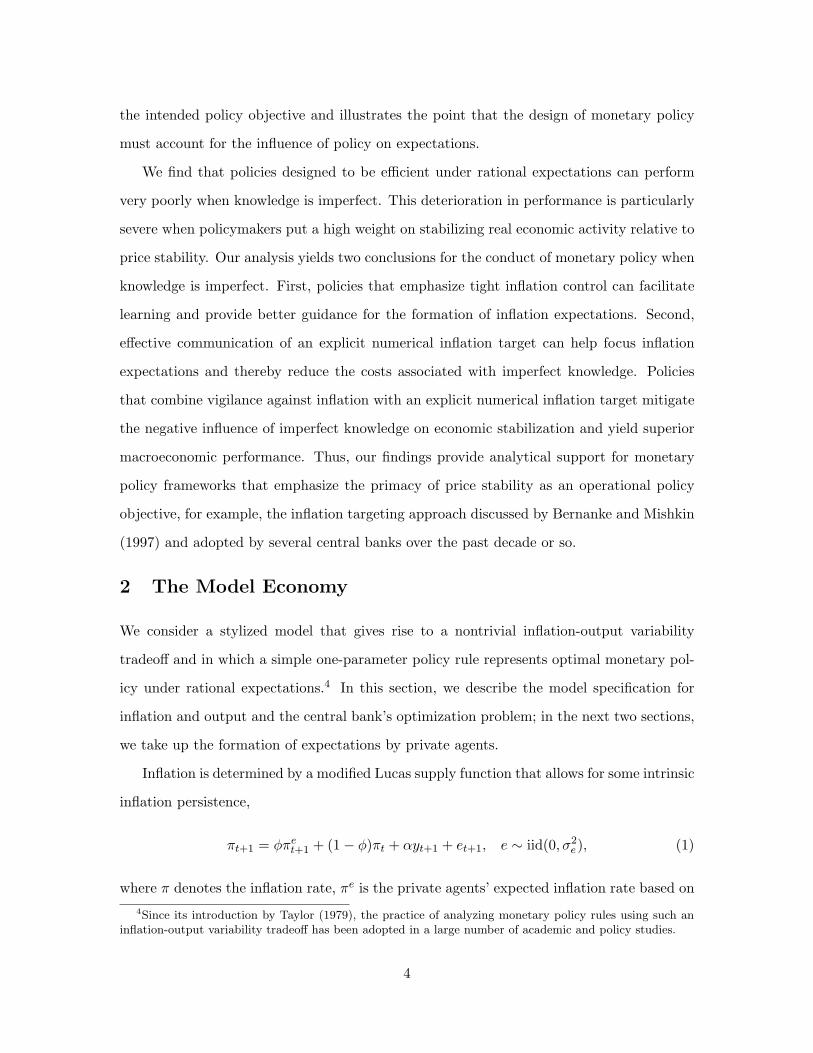
Inflation is determined by a modified Lucas supply function that allows for some intrinsic

inflation persistence,

πt+1 = φπet+1 + (1− φ)πt + αyt+1 + et+1, e ∼ iid(0, σ2

e), (1)

where π denotes the inflation rate, πe is the private agents’ expected inflation rate based on4Since its introduction by Taylor (1979), the practice of analyzing monetary policy rules using such an

inflation-output variability tradeoff has been adopted in a large number of academic and policy studies.

4

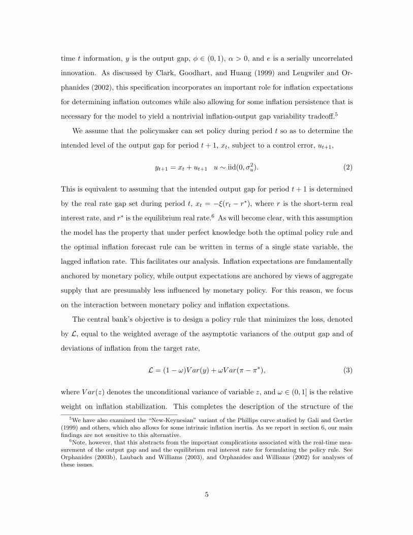
time t information, y is the output gap, φ ∈ (0, 1), α > 0, and e is a serially uncorrelated

innovation. As discussed by Clark, Goodhart, and Huang (1999) and Lengwiler and Or-

phanides (2002), this specification incorporates an important role for inflation expectations

for determining inflation outcomes while also allowing for some inflation persistence that is

necessary for the model to yield a nontrivial inflation-output gap variability tradeoff.5

We assume that the policymaker can set policy during period t so as to determine the

intended level of the output gap for period t + 1, xt, subject to a control error, ut+1,

yt+1 = xt + ut+1 u ∼ iid(0, σ2u). (2)

This is equivalent to assuming that the intended output gap for period t + 1 is determined

by the real rate gap set during period t, xt = −ξ(rt − r∗), where r is the short-term real

interest rate, and r∗ is the equilibrium real rate.6 As will become clear, with this assumption

the model has the property that under perfect knowledge both the optimal policy rule and

the optimal inflation forecast rule can be written in terms of a single state variable, the

lagged inflation rate. This facilitates our analysis. Inflation expectations are fundamentally

anchored by monetary policy, while output expectations are anchored by views of aggregate

supply that are presumably less influenced by monetary policy. For this reason, we focus

on the interaction between monetary policy and inflation expectations.

The central bank’s objective is to design a policy rule that minimizes the loss, denoted

by L, equal to the weighted average of the asymptotic variances of the output gap and of

deviations of inflation from the target rate,

L = (1− ω)V ar(y) + ωV ar(π − π∗), (3)

where V ar(z) denotes the unconditional variance of variable z, and ω ∈ (0, 1] is the relative

weight on inflation stabilization. This completes the description of the structure of the5We have also examined the “New-Keynesian” variant of the Phillips curve studied by Gali and Gertler

(1999) and others, which also allows for some intrinsic inflation inertia. As we report in section 6, our mainfindings are not sensitive to this alternative.

6Note, however, that this abstracts from the important complications associated with the real-time mea-surement of the output gap and and the equilibrium real interest rate for formulating the policy rule. SeeOrphanides (2003b), Laubach and Williams (2003), and Orphanides and Williams (2002) for analyses ofthese issues.

5

model economy, with the exception of the expectations formation process that we examine

in detail below.

3 The Perfect Knowledge Benchmark

We begin by considering the “textbook” case of rational expectations with perfect knowl-

edge in which private agents know both the structure of the economy and the central bank’s

policy. In this case, expectations are rational in that they are consistent with the true data

generating process of the economy (the model). In the next section, we use the result-

ing equilibrium solution as a “perfect knowledge” benchmark against which we compare

outcomes under imperfect knowledge, in which case agents do not know the structural pa-

rameters of the model but instead must form expectations based on estimated forecasting

models.

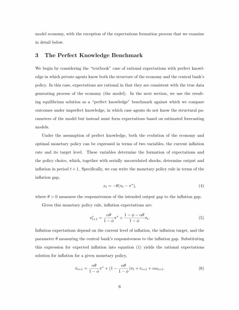
Under the assumption of perfect knowledge, both the evolution of the economy and

optimal monetary policy can be expressed in terms of two variables, the current inflation

rate and its target level. These variables determine the formation of expectations and

the policy choice, which, together with serially uncorrelated shocks, determine output and

inflation in period t + 1. Specifically, we can write the monetary policy rule in terms of the

inflation gap,

xt = −θ(πt − π∗), (4)

where θ > 0 measures the responsiveness of the intended output gap to the inflation gap.

Given this monetary policy rule, inflation expectations are:

πet+1 =

αθ

1− φπ∗ +

1− φ− αθ

1− φπt. (5)

Inflation expectations depend on the current level of inflation, the inflation target, and the

parameter θ measuring the central bank’s responsiveness to the inflation gap. Substituting

this expression for expected inflation into equation (1) yields the rational expectations

solution for inflation for a given monetary policy,

πt+1 =αθ

1− φπ∗ + (1− αθ

1− φ)πt + et+1 + αut+1. (6)

6

One noteworthy feature of this solution is that the first-order autocorrelation of the inflation

rate, given by 1− αθ1−φ , is decreasing in θ and is invariant to the value of π∗. Note that the

rational expectations solution can also be written in terms of the “inflation expectations

gap”—the difference between inflation expectations for period t+1 from the inflation target,

πet+1 − π∗t ,

πet+1 − π∗t =

1− φ− αθ

1− φ(πt − π∗). (7)

Equations (4) and (5) close the perfect knowledge benchmark model.

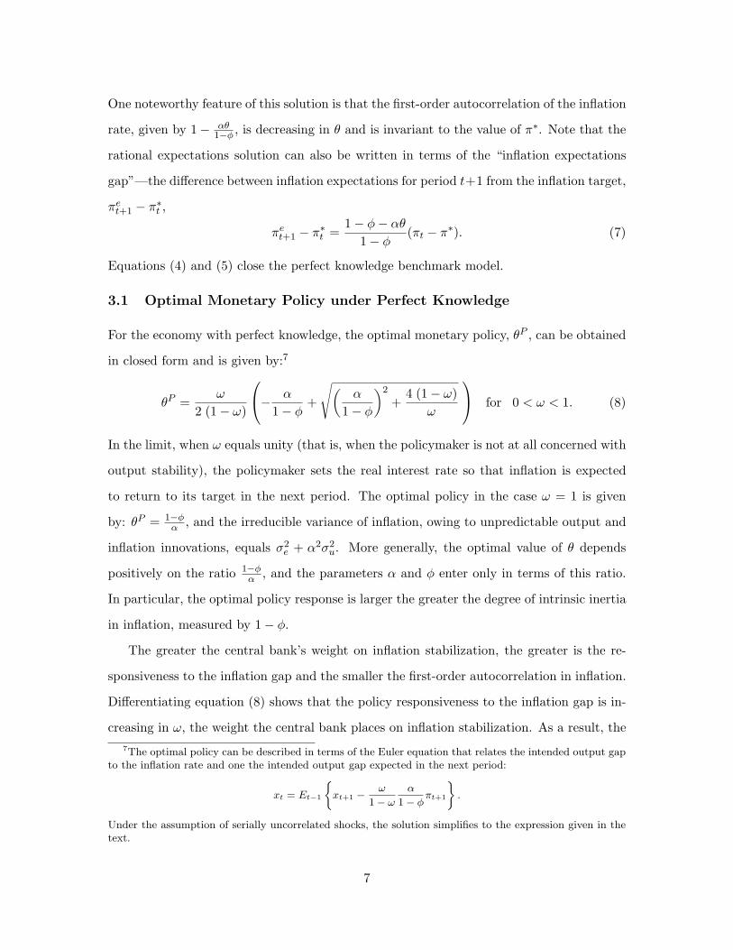
3.1 Optimal Monetary Policy under Perfect Knowledge

For the economy with perfect knowledge, the optimal monetary policy, θP , can be obtained

in closed form and is given by:7

θP =ω

2 (1− ω)

− α

1− φ+

√(α

1− φ

)2

+4 (1− ω)

ω

for 0 < ω < 1. (8)

In the limit, when ω equals unity (that is, when the policymaker is not at all concerned with

output stability), the policymaker sets the real interest rate so that inflation is expected

to return to its target in the next period. The optimal policy in the case ω = 1 is given

by: θP = 1−φα , and the irreducible variance of inflation, owing to unpredictable output and

inflation innovations, equals σ2e + α2σ2

u. More generally, the optimal value of θ depends

positively on the ratio 1−φα , and the parameters α and φ enter only in terms of this ratio.

In particular, the optimal policy response is larger the greater the degree of intrinsic inertia

in inflation, measured by 1− φ.

The greater the central bank’s weight on inflation stabilization, the greater is the re-

sponsiveness to the inflation gap and the smaller the first-order autocorrelation in inflation.

Differentiating equation (8) shows that the policy responsiveness to the inflation gap is in-

creasing in ω, the weight the central bank places on inflation stabilization. As a result, the7The optimal policy can be described in terms of the Euler equation that relates the intended output gap

to the inflation rate and one the intended output gap expected in the next period:

xt = Et−1

{xt+1 − ω

1− ω

α

1− φπt+1

}.

Under the assumption of serially uncorrelated shocks, the solution simplifies to the expression given in thetext.

7

autocorrelation of inflation is decreasing in ω, with a limiting value approaching unity when

ω approaches zero, and zero when ω equals one. That is, if the central bank cares only

about output stabilization, the inflation rate becomes a random walk, while if the central

bank cares only about inflation stabilization, the inflation rate displays no serial correlation.

And, as noted, this model yields a nontrivial monotonic tradeoff between the variability of

inflation and the output gap for all values of ω ∈ (0, 1]. These results are illustrated in

Figure 1. The top panel of the figure shows the variability tradeoff described by optimal

policies for values of ω between zero and one. The lower panel plots the optimal values of

θ against ω.

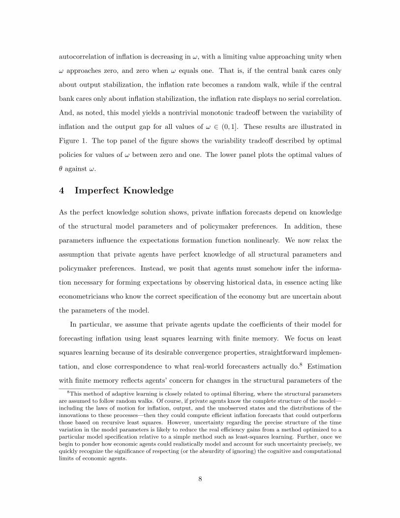
4 Imperfect Knowledge

As the perfect knowledge solution shows, private inflation forecasts depend on knowledge

of the structural model parameters and of policymaker preferences. In addition, these

parameters influence the expectations formation function nonlinearly. We now relax the

assumption that private agents have perfect knowledge of all structural parameters and

policymaker preferences. Instead, we posit that agents must somehow infer the informa-

tion necessary for forming expectations by observing historical data, in essence acting like

econometricians who know the correct specification of the economy but are uncertain about

the parameters of the model.

In particular, we assume that private agents update the coefficients of their model for

forecasting inflation using least squares learning with finite memory. We focus on least

squares learning because of its desirable convergence properties, straightforward implemen-

tation, and close correspondence to what real-world forecasters actually do.8 Estimation

with finite memory reflects agents’ concern for changes in the structural parameters of the8This method of adaptive learning is closely related to optimal filtering, where the structural parameters

are assumed to follow random walks. Of course, if private agents know the complete structure of the model—including the laws of motion for inflation, output, and the unobserved states and the distributions of theinnovations to these processes—then they could compute efficient inflation forecasts that could outperformthose based on recursive least squares. However, uncertainty regarding the precise structure of the timevariation in the model parameters is likely to reduce the real efficiency gains from a method optimized to aparticular model specification relative to a simple method such as least-squares learning. Further, once webegin to ponder how economic agents could realistically model and account for such uncertainty precisely, wequickly recognize the significance of respecting (or the absurdity of ignoring) the cognitive and computationallimits of economic agents.

8

economy. To focus our attention on the role of imperfections in the expectations formation

process itself, however, we deliberately abstract from the introduction of the actual uncer-

tainty in the structure of the economy which would justify such concerns in equilibrium.

Further, we do not model the policymaker’s knowledge or learning, but instead focus on the

implications of policy based on simple time-invariant rules of the form given in equation (4)

that do not require explicit treatment of the policymaker’s learning problem.9

We model perpetual learning by assuming that agents use a constant gain in their

recursive least squares formula that places greater weight on more recent observations,

as in Sargent (1999) and Evans and Honkapohja (2001). This algorithm is equivalent to

applying weighted least squares where the weights decline geometrically with the distance

in time between the observation being weighted and the most recent observation. This

approach is closely related to the use of fixed sample lengths or rolling-window regressions

to estimate a forecasting model (Friedman 1979). In terms of the mean “age” of the data

used, a rolling-regression window of length l is equivalent to a constant gain κ of 2/l. The

advantage of the constant gain least squares algorithm over rolling regressions is that the

evolution of the former system is fully described by a small set of variables, while the latter

requires one to keep track of a large number of variables.

4.1 Least Squares Learning with Finite Memory

Under perfect knowledge, the predictable component of next period’s inflation rate is a linear

function of the inflation target and the current inflation rate, where the coefficients on the

two variables are functions of the policy parameter θ and the other structural parameters

of the model, as shown in equation (5). In addition, the optimal value of θ is itself a

nonlinear function of the central bank’s weight on inflation stabilization and the other

model structural parameters. Given this simple structure, the least squares regression of

inflation on a constant and lagged inflation,

πi = c0,t + c1,tπi−1 + vi, (9)

9We also abstract from two other elements that may further complicate policy design: The possibilitiesthat policymakers may rely on a misspecified model or a misspecified information set for computing agent’sexpectations; see, Levin, Wieland, and Williams (2003) and Orphanides (2003b), respectively, for a discussionof these two issues.

9

yields consistent estimates of the coefficients describing the law of motion for inflation

(Marcet and Sargent 1988 and Evans and Honkapohja 2001). Agents then use these results

to form their inflation expectations.10

To fix notation, let Xi and ci be the 2 × 1 vectors Xi = (1, πi−1)′ and ci = (c0,i, c1,i)′.

Using data through period t, the least squares regression parameters for equation (9) can

be written in recursive form:

ct = ct−1 + κtR−1t Xt(πt −X ′

tct−1), (10)

Rt = Rt−1 + κt(XtX′t −Rt−1), (11)

where κt is the gain. With least squares learning with infinite memory, κt = 1/t, so as

t increases, κt converges to zero. As a result, as the data accumulate this mechanism

converges to the correct expectations functions and the economy converges to the perfect

knowledge benchmark solution. As noted above, to formalize perpetual learning—as would

be required in the presence of structural change—we replace the decreasing gain in the

infinite memory recursion with a small constant gain, κ > 0.11

With imperfect knowledge, expectations are based on the perceived law of motion of

the inflation process, governed by the perpetual learning algorithm described above. The

model under imperfect knowledge consists of the structural equation for inflation (1), the

output gap equation (2), the monetary policy rule (4), and the one-step-ahead forecast for

inflation, given by

πet+1 = c0,t + c1,tπt, (12)

where c0,t and c1,t are updated according to equations (10) and (11).

We emphasize that in the limit of perfect knowledge (that is, as κ → 0), the expectations

function above converges to rational expectations and the stochastic coefficients for the10Note that here we assume that agents employ a reduced form of the expectations formation function

that is correctly specified under rational expectations with perfect knowledge. However, agents may beuncertain of the correct form and estimate a more general specification, for example, a linear regression withadditional lags of inflation which nests (9). In section 6, we also discuss results from such an example.

11In terms of forecasting performance, the “optimal” choice of κ depends on the relative variances of thetransitory and permanent shocks, as in the relationship between the Kalman gain and the signal-to-noiseratio in the case of the Kalman filter. Here, we do not explicitly attempt to calibrate κ in this way, butinstead examine the effects for a range of values of κ.

10

intercept and slope collapse to:

cP0 =

αθπ∗

1− φ,

cP1 =

1− φ− αθ

1− φ.

Thus, this modeling approach accommodates the Lucas critique in the sense that expec-

tations formation is endogenous and adjusts to changes in policy or structure (as reflected

here by changes in the parameters θ, π∗, α, and φ). In essence, our model is one of “noisy ra-

tional expectations.” As we show below, although expectations are imperfectly rational, in

that agents need to estimate the reduced form equations they employ to form expectations,

they are nearly rational, in that the forecasts are close to being efficient.

5 Perpetual Learning in Action

We use model simulations to illustrate how learning affects the dynamics of inflation ex-

pectations, inflation, and output in the model economy. First, we examine the behavior of

the estimated coefficients of the inflation forecast equation and evaluate the performance of

inflation forecasts. We then consider the dynamic response of the economy to shocks sim-

ilar to those experienced during the 1970s in the United States. Specifically, we compare

the outcomes under perfect knowledge and imperfect knowledge with least squares learn-

ing that correspond to three alternative monetary policy rules to illustrate the additional

layer of dynamic interaction introduced by the imperfections in the formation of inflation

expectations.

In calibrating the model for the simulations, each period corresponds to about half a

year. We consider values of κ of 0.025, 0.05, and 0.075, which roughly correspond to using

40, 20, or 13 years of data, respectively, in the context of rolling regressions. We consider

two values for φ, the parameter that measures the influence of inflation expectations on

inflation. As a baseline case, we set φ to 0.75, which implies a significant role for intrinsic

inflation inertia, consistent with the contracting models of Buiter and Jewitt (1981), and

Fuhrer and Moore (1995), and Brayton, et al. (1997).12 In the alternative specification, we12Other researchers suggest an even smaller role for expectations relative to intrinsic inertia; see Fuhrer

(1997), Roberts (2001), and Rudd and Whelan (2001).

11

allow for a greater role for expectations and correspondingly give less weight to inflation

inertia by setting φ = 0.9, consistent with the findings of Gali and Gertler (1999) and others.

To ease comparisons between the two values of φ, we set α so that the optimal policy under

perfect knowledge is identical in the two cases. Specifically, for φ = 0.75, we set α = 0.25,

and for φ = 0.9, we set α = 0.1. In all cases, we assume σe = σu = 1.

The three alternative policies we consider correspond to the values of θ, {0.1, 0.6, 1.0},which represent the optimal policies under perfect knowledge for policymakers whose pref-

erences reflect a relative weight on inflation, ω, of 0.01, 0.5, and 1, respectively. Hence,

θ = 0.1 corresponds to an “inflation dove” policymaker who is primarily concerned about

output stabilization, θ = 0.6 corresponds to a policymaker with “balanced preferences” who

weighs inflation and output stabilization equally, and θ = 1 corresponds to an “inflation

hawk” policymaker who cares exclusively about inflation.

5.1 The Performance of Least-Squares Inflation Forecasts

Even absent shocks to the structure of the economy, the process of least squares learn-

ing generates time variation in the formation of inflation expectations and thereby in the

processes of inflation and output. The magnitude of this time variation is increasing in κ—

which is equivalent to using shorter samples (and thus less information from the historical

data) in rolling regressions. Table 1 reports summary statistics of the estimates of agents’

inflation forecasting model based on stochastic simulations of the model economy for the

two calibrations we consider. As seen in the table, the unconditional standard deviations

of the estimates increase with κ. This dependence of the variation in the estimates on the

rate of learning is portrayed in Figure 2, which shows the steady-state distributions of the

estimates of c0 and c1 for the case of φ0.75. For comparison, the vertical lines in each panel

indicate the values of c0 and c1 in the corresponding perfect knowledge benchmark.

The median values of the coefficient estimates are nearly identical to the values implied

by the perfect knowledge benchmark; however, the mean estimates of c1 are biased down-

ward slightly. Although not shown in the table, the mean and median values of c0 are

nearly zero, consistent with the assumed inflation target of zero. There is contemporaneous

correlation between estimates of c0 and c1 is nearly zero. Each of these estimates, however,

12

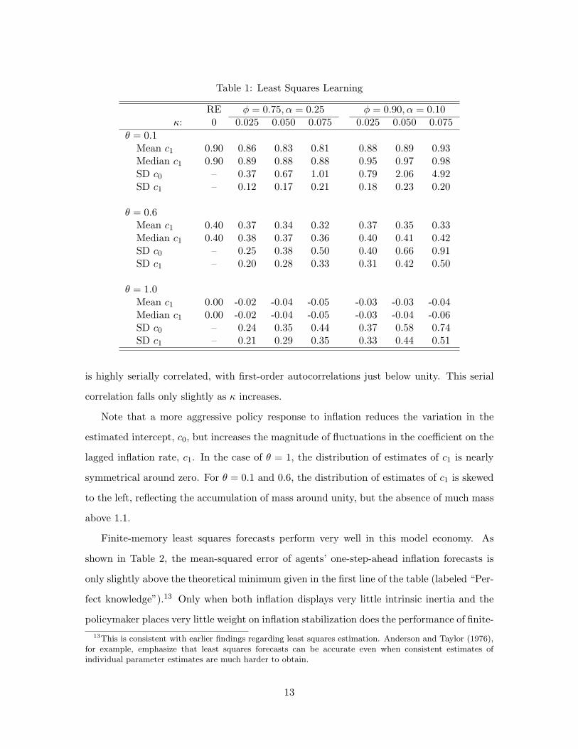
Table 1: Least Squares Learning

RE φ = 0.75, α = 0.25 φ = 0.90, α = 0.10κ: 0 0.025 0.050 0.075 0.025 0.050 0.075

θ = 0.1Mean c1 0.90 0.86 0.83 0.81 0.88 0.89 0.93Median c1 0.90 0.89 0.88 0.88 0.95 0.97 0.98SD c0 – 0.37 0.67 1.01 0.79 2.06 4.92SD c1 – 0.12 0.17 0.21 0.18 0.23 0.20

θ = 0.6Mean c1 0.40 0.37 0.34 0.32 0.37 0.35 0.33Median c1 0.40 0.38 0.37 0.36 0.40 0.41 0.42SD c0 – 0.25 0.38 0.50 0.40 0.66 0.91SD c1 – 0.20 0.28 0.33 0.31 0.42 0.50

θ = 1.0Mean c1 0.00 -0.02 -0.04 -0.05 -0.03 -0.03 -0.04Median c1 0.00 -0.02 -0.04 -0.05 -0.03 -0.04 -0.06SD c0 – 0.24 0.35 0.44 0.37 0.58 0.74SD c1 – 0.21 0.29 0.35 0.33 0.44 0.51

is highly serially correlated, with first-order autocorrelations just below unity. This serial

correlation falls only slightly as κ increases.

Note that a more aggressive policy response to inflation reduces the variation in the

estimated intercept, c0, but increases the magnitude of fluctuations in the coefficient on the

lagged inflation rate, c1. In the case of θ = 1, the distribution of estimates of c1 is nearly

symmetrical around zero. For θ = 0.1 and 0.6, the distribution of estimates of c1 is skewed

to the left, reflecting the accumulation of mass around unity, but the absence of much mass

above 1.1.

Finite-memory least squares forecasts perform very well in this model economy. As

shown in Table 2, the mean-squared error of agents’ one-step-ahead inflation forecasts is

only slightly above the theoretical minimum given in the first line of the table (labeled “Per-

fect knowledge”).13 Only when both inflation displays very little intrinsic inertia and the

policymaker places very little weight on inflation stabilization does the performance of finite-13This is consistent with earlier findings regarding least squares estimation. Anderson and Taylor (1976),

for example, emphasize that least squares forecasts can be accurate even when consistent estimates ofindividual parameter estimates are much harder to obtain.

13

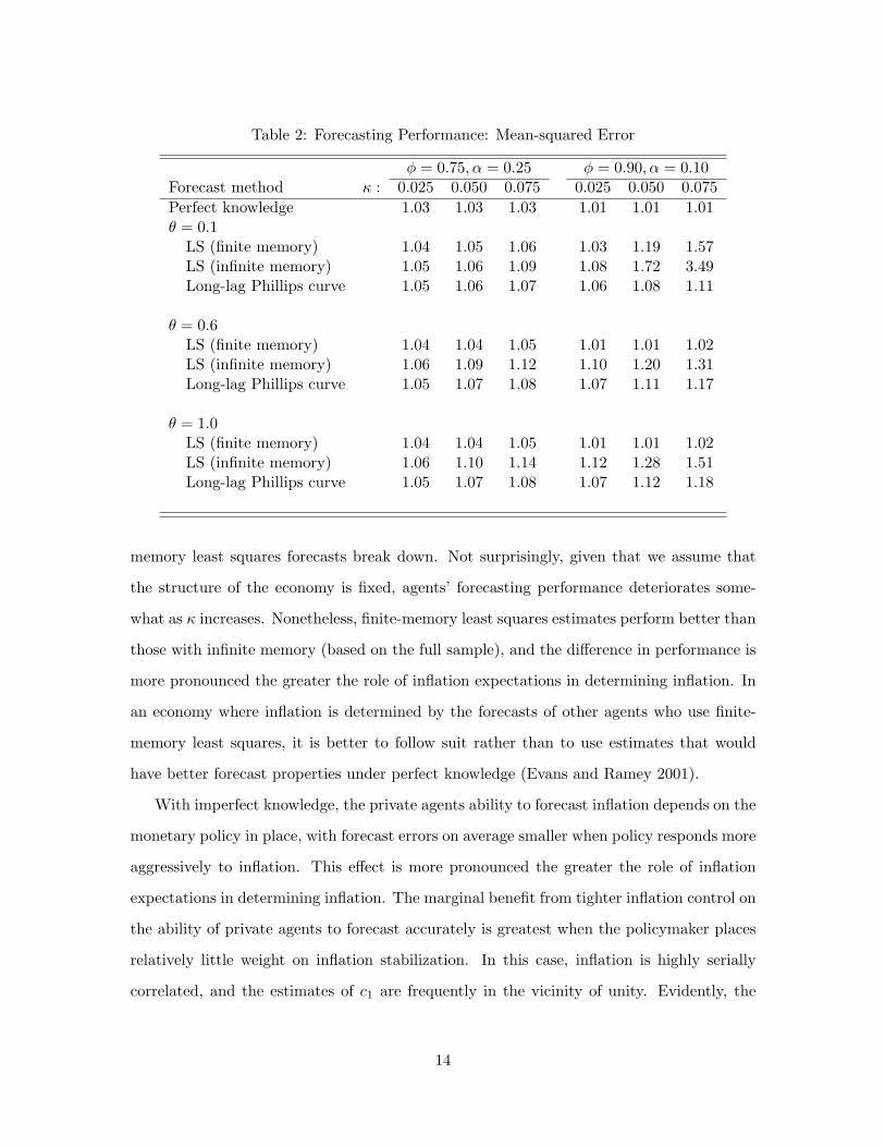
Table 2: Forecasting Performance: Mean-squared Error

φ = 0.75, α = 0.25 φ = 0.90, α = 0.10Forecast method κ : 0.025 0.050 0.075 0.025 0.050 0.075Perfect knowledge 1.03 1.03 1.03 1.01 1.01 1.01θ = 0.1

LS (finite memory) 1.04 1.05 1.06 1.03 1.19 1.57LS (infinite memory) 1.05 1.06 1.09 1.08 1.72 3.49Long-lag Phillips curve 1.05 1.06 1.07 1.06 1.08 1.11

θ = 0.6LS (finite memory) 1.04 1.04 1.05 1.01 1.01 1.02LS (infinite memory) 1.06 1.09 1.12 1.10 1.20 1.31Long-lag Phillips curve 1.05 1.07 1.08 1.07 1.11 1.17

θ = 1.0LS (finite memory) 1.04 1.04 1.05 1.01 1.01 1.02LS (infinite memory) 1.06 1.10 1.14 1.12 1.28 1.51Long-lag Phillips curve 1.05 1.07 1.08 1.07 1.12 1.18

memory least squares forecasts break down. Not surprisingly, given that we assume that

the structure of the economy is fixed, agents’ forecasting performance deteriorates some-

what as κ increases. Nonetheless, finite-memory least squares estimates perform better than

those with infinite memory (based on the full sample), and the difference in performance is

more pronounced the greater the role of inflation expectations in determining inflation. In

an economy where inflation is determined by the forecasts of other agents who use finite-

memory least squares, it is better to follow suit rather than to use estimates that would

have better forecast properties under perfect knowledge (Evans and Ramey 2001).

With imperfect knowledge, the private agents ability to forecast inflation depends on the

monetary policy in place, with forecast errors on average smaller when policy responds more

aggressively to inflation. This effect is more pronounced the greater the role of inflation

expectations in determining inflation. The marginal benefit from tighter inflation control on

the ability of private agents to forecast accurately is greatest when the policymaker places

relatively little weight on inflation stabilization. In this case, inflation is highly serially

correlated, and the estimates of c1 are frequently in the vicinity of unity. Evidently, the

14

ability to forecast inflation deteriorates when inflation is nearly a random walk. As seen

by comparing the cases of θ of 0.6 and 1.0, the marginal benefit of tight inflation control

disappears once the first-order autocorrelation of inflation is well below one.

Finally, even though only one lag of inflation appears in the equations for inflation and

inflation expectations, it is possible to improve on infinite-memory least squares forecasts

by including additional lags of inflation in the estimated forecasting equation. This result is

similar to that found in empirical studies of inflation, where relatively long lags of inflation

help predict inflation (Staiger, Stock, and Watson 1997, Stock and Watson 1999, Brayton,

Roberts, and Williams 1999). Evidently, in an economy where agents use adaptive learning,

multi-period lags of inflation are a reasonable proxy for inflation expectations. This result

may also help explain the finding that survey-based inflation expectations do not appear to

be “rational” using standard tests (Roberts 1997, 1998). With adaptive learning, inflation

forecast errors are correlated with data in the agents’ information set; the standard test for

forecast efficiency applies only to stable economic environments in which agents’ estimates

of the forecast model have converged to the true values.

5.2 Least Squares Learning and Inflation Persistence

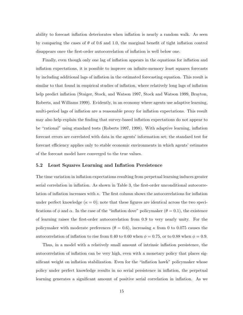
The time variation in inflation expectations resulting from perpetual learning induces greater

serial correlation in inflation. As shown in Table 3, the first-order unconditional autocorre-

lation of inflation increases with κ. The first column shows the autocorrelations for inflation

under perfect knowledge (κ = 0); note that these figures are identical across the two speci-

fications of φ and α. In the case of the “inflation dove” policymaker (θ = 0.1), the existence

of learning raises the first-order autocorrelation from 0.9 to very nearly unity. For the

policymaker with moderate preferences (θ = 0.6), increasing κ from 0 to 0.075 causes the

autocorrelation of inflation to rise from 0.40 to 0.60 when φ = 0.75, or to 0.88 when φ = 0.9.

Thus, in a model with a relatively small amount of intrinsic inflation persistence, the

autocorrelation of inflation can be very high, even with a monetary policy that places sig-

nificant weight on inflation stabilization. Even for the “inflation hawk” policymaker whose

policy under perfect knowledge results in no serial persistence in inflation, the perpetual

learning generates a significant amount of positive serial correlation in inflation. As we

15

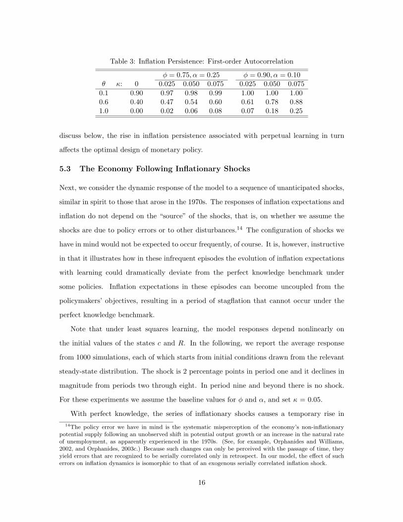
Table 3: Inflation Persistence: First-order Autocorrelation

φ = 0.75, α = 0.25 φ = 0.90, α = 0.10θ κ: 0 0.025 0.050 0.075 0.025 0.050 0.075

0.1 0.90 0.97 0.98 0.99 1.00 1.00 1.000.6 0.40 0.47 0.54 0.60 0.61 0.78 0.881.0 0.00 0.02 0.06 0.08 0.07 0.18 0.25

discuss below, the rise in inflation persistence associated with perpetual learning in turn

affects the optimal design of monetary policy.

5.3 The Economy Following Inflationary Shocks

Next, we consider the dynamic response of the model to a sequence of unanticipated shocks,

similar in spirit to those that arose in the 1970s. The responses of inflation expectations and

inflation do not depend on the “source” of the shocks, that is, on whether we assume the

shocks are due to policy errors or to other disturbances.14 The configuration of shocks we

have in mind would not be expected to occur frequently, of course. It is, however, instructive

in that it illustrates how in these infrequent episodes the evolution of inflation expectations

with learning could dramatically deviate from the perfect knowledge benchmark under

some policies. Inflation expectations in these episodes can become uncoupled from the

policymakers’ objectives, resulting in a period of stagflation that cannot occur under the

perfect knowledge benchmark.

Note that under least squares learning, the model responses depend nonlinearly on

the initial values of the states c and R. In the following, we report the average response

from 1000 simulations, each of which starts from initial conditions drawn from the relevant

steady-state distribution. The shock is 2 percentage points in period one and it declines in

magnitude from periods two through eight. In period nine and beyond there is no shock.

For these experiments we assume the baseline values for φ and α, and set κ = 0.05.

With perfect knowledge, the series of inflationary shocks causes a temporary rise in14The policy error we have in mind is the systematic misperception of the economy’s non-inflationary

potential supply following an unobserved shift in potential output growth or an increase in the natural rateof unemployment, as apparently experienced in the 1970s. (See, for example, Orphanides and Williams,2002, and Orphanides, 2003c.) Because such changes can only be perceived with the passage of time, theyyield errors that are recognized to be serially correlated only in retrospect. In our model, the effect of sucherrors on inflation dynamics is isomorphic to that of an exogenous serially correlated inflation shock.

16

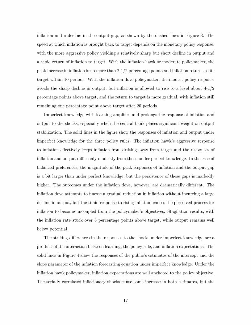
inflation and a decline in the output gap, as shown by the dashed lines in Figure 3. The

speed at which inflation is brought back to target depends on the monetary policy response,

with the more aggressive policy yielding a relatively sharp but short decline in output and

a rapid return of inflation to target. With the inflation hawk or moderate policymaker, the

peak increase in inflation is no more than 2-1/2 percentage points and inflation returns to its

target within 10 periods. With the inflation dove policymaker, the modest policy response

avoids the sharp decline in output, but inflation is allowed to rise to a level about 4-1/2

percentage points above target, and the return to target is more gradual, with inflation still

remaining one percentage point above target after 20 periods.

Imperfect knowledge with learning amplifies and prolongs the response of inflation and

output to the shocks, especially when the central bank places significant weight on output

stabilization. The solid lines in the figure show the responses of inflation and output under

imperfect knowledge for the three policy rules. The inflation hawk’s aggressive response

to inflation effectively keeps inflation from drifting away from target and the responses of

inflation and output differ only modestly from those under perfect knowledge. In the case of

balanced preferences, the magnitude of the peak responses of inflation and the output gap

is a bit larger than under perfect knowledge, but the persistence of these gaps is markedly

higher. The outcomes under the inflation dove, however, are dramatically different. The

inflation dove attempts to finesse a gradual reduction in inflation without incurring a large

decline in output, but the timid response to rising inflation causes the perceived process for

inflation to become uncoupled from the policymaker’s objectives. Stagflation results, with

the inflation rate stuck over 8 percentage points above target, while output remains well

below potential.

The striking differences in the responses to the shocks under imperfect knowledge are a

product of the interaction between learning, the policy rule, and inflation expectations. The

solid lines in Figure 4 show the responses of the public’s estimates of the intercept and the

slope parameter of the inflation forecasting equation under imperfect knowledge. Under the

inflation hawk policymaker, inflation expectations are well anchored to the policy objective.

The serially correlated inflationary shocks cause some increase in both estimates, but the

17

implied increase in the inflation target peaks at only 0.3 percentage point (not shown in the

figure). Even for the moderate policymaker who accommodates some of the inflationary

shock for a time, the perceived inflation target rises by just one-half percentage point.

In contrast, under the inflation dove policymaker, the estimated persistence of inflation,

already very high owing to the policymaker’s desire to minimize output fluctuations while

responding to inflation shocks, rises steadily, approaching unity. With inflation temporarily

perceived to be a near-random walk with positive drift, agents expect inflation to continue

to rise. The policymaker’s attempts to constrain inflation are too weak to counteract this

adverse expectations process, and the public’s perception of the inflation target rises by 5

percentage points. Despite the best of intents, the gradual disinflation prescription that

would be optimal with perfect knowledge yields stagflation—the simultaneous occurrence

of persistently high inflation and low output.

Interestingly, the inflation dove simulation appears to capture some key characteristics

of the United States economy at the end of the 1970s, and it accords well with Chairman

Volcker’s assessment of the economic situation at the time:

Moreover, inflationary expectations are now deeply embedded in public atti-tudes, as reflected in the practices and policies of individuals and economicinstitutions. After years of false starts in the effort against inflation, there iswidespread skepticism about the prospects for success. Overcoming this legacyof doubt is a critical challenge that must be met in shaping–and in carryingout–all our policies.

Changing both expectations and actual price performance will be difficult. Butit is essential if our economic future is to be secure.(Volcker 1981, p. 293)

In contrast to this dismal experience, the model simulations suggest that the rise in inflation—

and the corresponding costs of disinflation—would have been much smaller if policy had

responded more aggressively to the inflationary developments of the 1970s. Although this

was apparently not recognized at the time, Chairman Volcker’s analysis suggests that the

stagflationary experience of the 1970s played a role in the subsequent recognition of the

value of continued vigilance against inflation in anchoring inflation expectations.

18

6 Imperfect Knowledge and Monetary Policy

6.1 Naive Application of the Rational Expectations Policy

We now turn to the design of efficient monetary policy under imperfect knowledge. We start

by considering the experiment in which the policymaker sets policy under the assumption

that private agents have perfect knowledge when, in fact, they have only imperfect knowl-

edge and base their expectations on the perpetual learning mechanism described above.

That is, policy follows (4) with the response parameter, θ, computed using (8).

Figure 5 compares the variability pseudo-frontier corresponding to this equilibrium to

the frontier from the perfect knowledge benchmark. The top panel shows the outcomes in

terms of inflation and output gap variability with the baseline parameterization, φ = 0.75.

The bottom panel shows the results of the same experiment with the more forward-looking

specification for inflation, φ = 0.9. In each case, we show the imperfect knowledge equilibria

corresponding to three different values of κ.

With imperfect knowledge, the perpetual learning mechanism introduces random errors

in expectations formation, that is, deviations of expectations from the values that would

correspond to the same realization of inflation and the same policy rule. These errors are

costly for stabilization and are responsible for the deterioration in performance shown in

Figure 5.

This deterioration in performance is especially pronounced for the policymaker who

places relatively low weight on inflation stabilization. As seen in the simulations of the

inflationary shocks reported above, for such policies the time variation in the estimated au-

tocorrelation of inflation in the vicinity of unity associated with learning can be especially

costly. Furthermore, the deterioration in performance relative to the case of the perfect

knowledge benchmark is larger the greater is the role of expectations in determining infla-

tion. With the higher value for φ, if a policymaker’s preference for inflation stabilization is

too low, the resulting outcomes under imperfect knowledge are strictly dominated by the

outcomes corresponding to the naive policy equilibrium for higher values of ω.

19

6.2 Efficient Simple Rule

Next we examine imperfect knowledge equilibria when the policymaker is aware of the im-

perfection in expectations formation and adjusts policy accordingly. To allow for a straight-

forward comparison with the perfect knowledge benchmark, we concentrate on the efficient

choice of the responsiveness of policy to inflation, θS , in the simple linear rule:

xt = −θS(πt − π∗),

which has the same form as the optimal rule under the perfect knowledge benchmark.15

The efficient policy response with imperfect knowledge is to be more vigilant against

inflation deviations from the policymaker’s target relative to the optimal response under

perfect knowledge. Figure 6 shows the efficient choices for θ under imperfect knowledge

for the two model parameterizations; the optimal policy under perfect knowledge—which

is the same for the two parameterizations considered—is shown again for comparison. As

before, we present results for three different values of κ, our baseline κ = 0.05 and also a

smaller and a larger value. The increase in the efficient value of θ is especially pronounced

when the policymaker places relatively little weight on inflation stabilization, that is, when

inflation would exhibit high serial correlation under perfect knowledge. Under imperfect

knowledge, it is efficient for a policymaker to bias the response to inflation upward relative

to that implied by perfect knowledge. This effect is especially pronounced with the more

forward-looking inflation process. Consider, for instance, the baseline case κ = 0.05. In the

parameterization with φ = 0.9, it is never efficient to set θ below 0.6, the value that one

would choose under balanced preferences (ω = 0.5) under perfect knowledge.

Accounting for imperfect knowledge can significantly improve stabilization performance

relative to outcomes obtained when the policymaker naively adopts policies that are efficient

under perfect knowledge. Figure 7 compares the loss to the policymaker with perfect and

imperfect knowledge for different preferences ω. The top panel shows the outcomes for the15In Orphanides and Williams (2003), we explore policies that respond directly to private expectations of

inflation, in addition to actual inflation. These rules are not fully optimal; with imperfect knowledge, thefully optimal policy would be a nonlinear function of all the states of the system, including the elements ofc and R. However, implementation of such policies would assume the policymaker’s full knowledge of thestructure of the economy an assumption we find untenable in practice.

20

baseline parameterization, φ = 0.75, α = 0.25; the bottom panel reports the outcomes for

the alternative parameterization of inflation, φ = 0.9, α = 0.1. In both panels, the results we

show for imperfect knowledge correspond to our benchmark case, κ = 0.05. The payoff to

reoptimizing θ is largest for policymakers who place a large weight on output stabilization,

with the gain huge in the case of φ = 0.9. In contrast, the benefits from reoptimization are

trivial for policymakers who are primarily concerned with inflation stabilization regardless

of φ.

The key finding that the public’s imperfect knowledge raises the efficient policy response

to inflation is not unique to the model considered here and carries over to models with

alternative specifications. In particular, we find the same result when the equation for

inflation is replaced with the “New Keynesian” variant studied by Gali and Gertler (1999)

(see also Gaspar and Smets 2002). Moreover, we find that qualitatively similar results

obtain if agents include additional lags of inflation in their forecasting models.

6.3 Dissecting the Benefits of Vigilance

In order to gain insight into the interaction of imperfections in the formation of expectations

and efficient policy, we consider a simple example where the parameters of the inflation

forecast model vary according to an exogenous stochastic process.

From equation (5), recall that expectations formation is driven by the stochastic coeffi-

cient expectations function:

πet+1 = c0,t + c1,tπt. (13)

For the present purposes, let c0,t and c1,t vary relative to their perfect knowledge benchmark

values; i.e., c0,t = cP0 + v0,t and c1,t = cP

1 + v1,t, where v0,t and v1,t are independent zero

mean normal distributions with variances σ20 and σ2

1.

Substituting expectations into the Phillips curve and rearranging terms results in the

following reduced form characterization of the dynamics of inflation in terms of the control

variable x:

πt+1 = (1 + φv1,t)πt +α

1− φxt + αut+1 + et+1 + φv0,t. (14)

In this case, the optimal policy with stochastic coefficients has the same linear structure

21

as the optimal policy with fixed coefficients and perfect knowledge, and the optimal policy

response is monotonically increasing in the variance σ21.

16

Although informative, the simple case examined above ignores the important effect of

the serial correlation in v0 and v1 that obtains under imperfect knowledge. The efficient

choice of θ cannot be written in closed form in the case of serially correlated processes for v0

and v1, but a set of stochastic simulations is informative. Consider the efficient choice of θ

for our benchmark economy with balanced preferences, ω = 0.5. Under perfect knowledge,

the optimal choice of θ is approximately 0.6. Instead, simulations assuming an exogenous

autoregressive process for either c0 or c1 with a variance and autocorrelation matching our

economy with imperfect knowledge suggest an efficient choice of θ approximately equal to

0.7—regardless of whether the variation is due to c0 or to c1. For comparison, with the

endogenous variation in the parameters in the economy with learning, the efficient choice

of θ is 0.75.

As noted earlier, for a fixed policy choice of policy responsiveness in the policy rule, θ,

the uncertainty in the process of expectations formation with imperfect knowledge raises

the persistence of the inflation process relative to the perfect knowledge case. This can

be seen by comparing the solid and dashed lines in the two panels of Figure 8, which plot

the persistence of inflation when policy follows the RE-optimal rule and agents have perfect

and imperfect knowledge (with κ = 0.05), respectively. This increase in inflation persistence

complicates stabilization efforts as it raises, on average, the output costs associated with

restoring price stability when inflation deviates from its target.

The key benefit of adopting greater vigilance against inflation deviations from the pol-

icymaker’s target in the presence of imperfect knowledge comes from reducing this excess16See Turnovsky (1977) and Craine (1979) for early applications of the well-known optimal control results

for this case. For our model, specifically, the optimal response can be written as:

θ =α(1− φ)s

(1− φ)(1− ω) + α2s,

where s is the positive root of the quadratic equation:

0 = ω(1− ω)(1− φ)2 + (ωα2 + (1− ω)(1− φ)2φ2σ21)s + (φ2σ2

1 − 1)α2s2.

While the optimal policy response to inflation deviations from target, θ, is independent of σ20 , the variance

of the v0,t differentiation reveals that it is increasing in σ21 , the variance of v1,t. As σ2

1 → 0, of course, thissolution collapses to the optimal policy with perfect knowledge.

22

serial persistence of inflation. More aggressive policies reduce the persistence of inflation,

thus facilitating its control. The resulting efficient choice of reduction in inflation persistence

is reflected by the dash-dot lines in Figure 8.

7 Learning with a Known Inflation Target

Throughout the preceding discussion and analysis, we have implicitly assumed that agents

do not rely on explicit knowledge regarding the policymaker’s objectives in forming expec-

tations. Arguably, this assumption best describes situations where a central bank does not

successfully communicate to the public an explicit numerical inflation target and, perhaps,

a clear weighting of its price and economic stability objectives. Since the adoption and clear

communication of an explicit numerical inflation target is one of the key characteristics of

inflation targeting regimes, it is of interest to explore the implications of this dimension

of inflation targeting in our model. To do so, we consider the case where the policymaker

explicitly communicates the ultimate inflation target to the public; that is, we assume that

the public exactly knows the value of π∗ and explicitly incorporates this information in

forming inflation expectations. Of course, even in an explicit inflation targeting regime, the

public may remain somewhat uncertain regarding the policymaker’s inflation target, π∗, so

that this assumption of a perfectly known inflation target may not be obtainable in practice

and may be seen as an illustrative limiting case.

The assumption of a known numerical inflation target simplifies the public’s inflation

forecasting problem. From equations (7) and (8), the reduced form equation for inflation

under rational expectations is given by:

πt+1 − π∗ = (1− αθ

1− φ)(πt − π∗) + et+1 + αut+1. (15)

With a known inflation target, the inflation forecasting model consistent with rational

expectations is simply:

πi − π∗ = c1,t(πi−1 − π∗) + vi. (16)

Note that this forecasting equation only the slope parameter, c1 is estimated; thus, in terms

of the forecasting equation, the assumption of a known inflation target corresponds to a zero

23

restriction on c0 (when the forecasting regression written in terms of deviations of inflation

from its target). As in the case of an unknown inflation target, constant gain versions of

equations (10) and (11) can be used to model the evolution of the formation of inflation

expectations in this case. The one-step-ahead forecast of inflation is given by:

πet+1 = π∗ + c1,t(πt − π∗), (17)

and again, in the limit of perfect knowledge (that is, as κ → 0), the expectations function

above converges to rational expectations with the slope coefficient cP1 = 1−φ−αθ

1−φ . This

formulation captures a key rationale for adopting an explicit inflation targeting regime:

to reduce the public’s uncertainty and possible confusion about the central bank’s precise

inflation objective and thereby to anchor the public’s inflation expectations to the central

bank’s objective.17

Eliminating uncertainty about the inflation target improves macroeconomic perfor-

mance, in terms of both inflation and output stability. The dotted lines in the upper

panel of Figure 9 trace the RE-policy pseudo-frontiers in the case of a known inflation

target. For comparison, the dashed lines show the pseudo-frontiers assuming that the in-

flation target is not known by the public (this repeats the curves shown in Figure 5 for our

benchmark case, κ = 0.05). Recall that the pseudo-frontier is obtained by evaluating the

performance of the economy under imperfect knowledge for the set of policies for ω ∈ (0, 1]

given by equation (8) that would be optimal under perfect knowledge. As seen in the figure,

economic outcomes are clearly more favorable when the inflation target is assumed to be

perfectly known than otherwise. Still, the resulting pseudo-frontiers lie well to the northeast

of those that would obtain under perfect knowledge. Evidently, imperfect knowledge of the

dynamic process for inflation alone has large costs in terms of performance, especially when

expectations are very important for determining inflation outcomes, represented by the case

of φ = 0.9.17The adoption of inflation targeting may affect the private formation of expectations in other ways than

by tying down the ultimate inflation objective. For instance, Svensson (2002) argues that inflation-targetingcentral banks should also make explicit their preference weighting, ω, which in principle could furtherreduce the public’s uncertainty about policy objectives. However, given the remaining uncertainty aboutmodel parameters (α and φ in our model), the uncertainty about the value of c1 is not eliminated in thiscase. The extent to which this uncertainty may be reduced is left to further research.

24

The basic finding that, relative to the perfect knowledge benchmark, policy should be

more vigilant against inflation under imperfect knowledge also obtains in the case of a known

inflation target. The lower panels of Figure 9 show the optimal values of θ for the three

cases we consider: perfect knowledge, imperfect knowledge with known π∗, and imperfect

knowledge with unknown π∗. When π∗ is known, the optimal choice of θ is slightly lower

than when π∗ is unknown. Even with a known inflation target, however, it remains optimal

to be more vigilant against inflation relative to the perfect knowledge case. An exception

is the extreme case of ω = 1 when the optimal value of θ is exactly unity, the same value

that obtains under perfect knowledge.18

A striking result, seen most clearly in the case of φ = 0.9, is that the optimal value of θ

is relatively insensitive over a large range of values for the stabilization preference weight,

ω, whether the inflation is known or unknown. By contrast, under perfect knowledge, the

optimal value of θ is quite sensitive to ω. An implication of this finding is that with imperfect

knowledge, there is relatively little “cost” associated with policies designed as if inflation

were the central bank’s primary objective, even when policymakers place substantial value

in reducing output variability in fact. By contrast, as shown above, the costs of optimizing

policies that incorrectly place a large weight on output stability under the assumption

of perfect knowledge can be quite large. This asymmetry suggests that the practice of

concentrating attention primarily on price stability in the formulation of monetary policy

may be seen as a robust strategy for achieving both a high degree of price stability and a

high degree of economic stability.

8 Conclusion

We examine the effects of a relatively modest deviation from rational expectations resulting

from perpetual learning on the part of economic agents with imperfect knowledge. The pres-

ence of imperfections in the formation of expectations makes the monetary policy problem

considerably more difficult than would appear under rational expectations. Using a simple18In this limiting case, estimates of c1 are symmetrically distributed around zero. Hence, in terms of a

simple rule of the form given by equation 4, there is no gain from over-responding, relative to the case ofperfect knowledge, to actual inflation.

25

linear model, we show that although inflation expectations are nearly efficient, imperfect

knowledge raises the persistence of inflation and distorts the policymaker’s tradeoff between

inflation and output stabilization. As a result, policies that appear efficient under rational

expectations can result in economic outcomes significantly worse than would be expected

by analysis based on the assumption of perfect knowledge. The costs of failing to account

for the presence of imperfect knowledge are particularly pronounced for policymakers who

place a relatively greater value on stabilizing output: A strategy emphasizing tight inflation

control can yield superior economic performance, in terms of both inflation and output sta-

bility, than can policies that appear efficient under rational expectations. More generally,

policies emphasizing tight inflation control reduce the persistence of inflation and the inci-

dence of large deviations of expectations from the policy objective, thereby mitigating the

influence of imperfect knowledge on the economy. In addition, tighter control of inflation

makes the economy less prone to costly stagflationary episodes.

The adoption and effective communication of an explicit numerical inflation target also

mitigate the influence of imperfect knowledge on the economy. Communication of an in-

flation target may greatly improve attainable macroeconomic outcomes and afford greater

economic stability relative to the outcomes that are attainable when the public perceives

the policymaker’s ultimate inflation objective less clearly. These results highlight the po-

tential value of communicating central bank’s inflation objective and of continued vigilance

against inflation in anchoring inflation expectations and fostering macroeconomic stability.

26

References

Anderson, T. W. and Taylor, John B. “Some Experimental Results on the Statistical Prop-erties of Least Squares Estimates in Control Problems.” Econometrica, November 1976,44(6), pp. 1289–1302.

Ball, Laurence. “Near-Rationality and Inflation in Two Monetary Regimes.” NBER Work-ing Paper 7988, October 2000.

Balvers, Ronald J. and Cosimano, Thomas F. “Inflation Variability and Gradualist Mone-tary Policy.” The Review of Economic Studies, October 1994, 61(4), pp. 721–738.

Bernanke, Ben S. and Mishkin, Frederic S. “Inflation Targeting: A New Framework forMonetary Policy?” Journal of Economic Perspectives, Spring 1997, 11(2), pp. 97–116.

Blume, Lawrence E. and Easley, David. “Learning to Be Rational.” Journal of EconomicTheory, April 1982, 26(2), pp. 340–351.

Bomfim, Antulio; Tetlow, Robert; von zur Muehlen, Peter and Williams, John. “Expecta-tions, Learning and the Costs of Disinflation: Experiments Using the FRB/US Model.”in Topics in Monetary Policy Modeling, Bank for International Settlements, 1997, 5.

Bray, Margaret M. “Learning, Estimation, and the Stability of Rational Expectations.”Journal of Economic Theory, April 1982, 26(2), pp. 318–339.

Bray, Margaret M. “Convergence to Rational Expectations Equilibrium.” in Roman Fry-dman and Edmund S. Phelps, eds., Individual Forecasting and Aggregate Outcomes.Cambridge: Cambridge University Press, 1983.

Bray, Margaret M. and Savin, Nathan E. “Rational Expectations Equilibria, Learning, andModel Specification.” Econometrica, September 1984, 54(5), pp. 1129–1160.

Brayton, Flint; Mauskopf, Eileen; Reifschneider, David; Tinsley, Peter and Williams, John.“The Role of Expectations in the FRB/US Macroeconomic Model.” Federal ReserveBulletin, April 1997, 83(4), pp. 227–245.

Brayton, Flint; Roberts, John M. and Williams, John C. “What’s Happened to the PhillipsCurve?” Federal Reserve Board Finance and Economics Discussion Series WorkingPaper 1999-49, September 1999.

Buiter, Willem H. and Jewitt, Ian. “Staggered Wage Setting with Real Wage Relativities:Variations on a Theme by Taylor.” The Manchester School, September 1981, 49(3), pp.211–228.

Bullard, James B. and Mitra, Kaushik. “Learning About Monetary Policy Rules.” Journalof Monetary Economics, September 2002, 49(6), 1105-1129.

Carroll, Christopher D. “Macroeconomic Expectations of Households and Professional Fore-casters.” Quarterly Journal of Economics, February 2003, 118 (1), pp. 269–98.

Christiano Lawrence J. and Gust, Christopher. “The Expectations Trap Hypothesis.” inMoney, Monetary Policy and Transmission Mechanisms. Ottawa: Bank of Canada,2000.

Clark, Peter; Goodhart Charles A. E. and Huang, Haizhou. “Optimal Monetary Policy

27

Rules in a Rational Expectations Model of the Phillips Curve.” Journal of MonetaryEconomics, April 1999, 43(2), pp. 497–520.

Craine, Roger. “Optimal Monetary Policy with Uncertainty.” Journal of Economic Dy-namics and Control, 1979, 1(1), pp. 59–83.

Erceg, Christopher J. and Levin, Andrew T. “Imperfect Credibility and Inflation Persis-tence.” Journal of Monetary Economics, May 2003, 50(4), pp. 721–944.

Evans, George and Honkapohja, Seppo. Learning and Expectations in Macroeconomics.Princeton: Princeton University Press, 2001.

Evans, George and Ramey, Garey. “Adaptive Expectations, Underparameterization andthe Lucas Critique.” University of Oregon mimeo, May 2001.

Friedman, Benjamin M. “Optimal Expectations and the Extreme Information Assumptionsof ‘Rational Expectations’ Macromodels.” Journal of Monetary Economics, January1979, 5(1), pp. 23–41.

Fuhrer, Jeffrey C. “The (Un)Importance of Forward-looking Behavior in Price Specifica-tions.” Journal of Money, Credit and Banking, August 1997, 29(3), pp. 338–350.

Fuhrer, Jeffrey C. and Moore, George. “Inflation Persistence.” Quarterly Journal of Eco-nomics, February 1995, 110(1), pp. 127–59.

Gali, Jordi and Gertler, Mark. “Inflation Dynamics: A Structural Economic Analysis.”Journal of Monetary Economics, October 1999, 44(2), pp. 195–222.

Gaspar, Vitor and Smets, Frank. “Monetary Policy, Price Stability and Output Gap Sta-bilisation.” International Finance, Summer 2002, 5(2), pp. 193–211.

Kozicki, Sharon and Tinsley, Peter A. “What Do You Expect? Imperfect Policy Credibil-ity and Tests of the Expectations Hypothesis.” Federal Reserve Bank of Kansas CityWorking Paper 01-02, April 2001.

Laubach, Thomas and Williams, John C. “Measuring the Natural Rate of Interest.” Reviewof Economics and Statistics, 2003, forthcoming.

Lengwiler, Yvan and Orphanides, Athanasios. “Optimal Discretion.” Scandinavian Journalof Economics, June 2002, 104(2), pp. 261–276.

Levin, Andrew; Wieland, Volker and Williams, John. “The Performance of Forecast-BasedMonetary Policy Rules under Model Uncertainty.” American Economic Review, June2003, 93(3), pp. 622–645.

Lucas, Robert E., Jr. “Adaptive Behavior and Economic Theory.” Journal of Business,October 1986, 59(4), S401-S426.

Mankiw, N. Gregory and Reis, Ricardo. “Sticky Information Versus Sticky Prices: A Pro-posal to Replace the New Keynesian Phillips Curve.” Quarterly Journal of Economics,November 2002, 117(4), 1295–1328.

Marcet, Albert and Sargent, Thomas. “The Fate of Systems with ‘Adaptive’ Expectations.”American Economic Review, May 1988, 78(2), pp. 168–172.

Marcet, Albert and Sargent, Thomas. “Convergence of Least Squares Learning Mechanisms

28

in Self Referential Linear Stochastic Models.” Journal of Economic Theory, August1989, 48(2), 337-368.

Muth, John F. “Rational Expectations and the Theory of Price Movements.” Econometrica,July 1961, 29, pp. 315–335.

Orphanides, Athanasios. “Monetary Policy Rules, Macroeconomic Stability and Inflation:A View from the Trenches.” Journal of Money, Credit and Banking, 2003a, forthcoming.

Orphanides, Athanasios. “Monetary Policy Evaluation with Noisy Information.” Journalof Monetary Economics, April 2003b, 50(3), pp. 605–631.

Orphanides, Athanasios. “The Quest for Prosperity Without Inflation.” Journal of Mone-tary Economics, April 2003c, 50(3), pp. 633–663.

Orphanides, Athanasios and Williams, John C. “Monetary Policy Rules with UnknownNatural Rates.” Brookings Papers on Economic Activity, 2:2002, pp. 63–145.

Orphanides, Athanasios and Williams, John C. “Inflation Scares and Forecast-Based Mon-etary Policy,” mimeo, March 2003.

Roberts, John M. “Is Inflation Sticky?” Journal of Monetary Economics, July 1997, 39(2),pp. 173–196.

Roberts, John M. “Inflation Expectations and the Transmission of Monetary Policy.” Fed-eral Reserve Board Finance and Economics Discussion Series 1998-43, October 1998.

Roberts, John M. “How Well Does the New Keynesian Sticky-Price Model Fit the Data?”Federal Reserve Board Finance and Economics Discussion Series 2001-13, February 2001.

Rudd, Jeremy and Whelan, Karl. “New Tests of the New-Keynesian Phillips Curve.”Federal Reserve Board Finance and Economics Discussion Series 2001-30, July 2001.

Sargent, Thomas J. Bounded Rationality in Macroeconomics. Oxford and New York: Ox-ford University Press, Clarendon Press, 1993.

Sargent, Thomas J. The Conquest of American Inflation. Princeton: Princeton UniversityPress, 1999.

Simon, Herbert A. “Rationality as Process and as Product of Thought.” American Eco-nomic Review, May 1978, 68(2), pp. 1–16.

Sims, Christopher. “Implications of Rational Inattention.” Journal of Monetary Eco-nomics, April 2003, 50(3), pp. 497–720.

Staiger, Douglas; Stock, James H. and Watson, Mark W. “How Precise are Estimates ofthe Natural Rate of Unemployment?” in Christina D. Romer and David H. Romer, eds.Reducing Inflation: Motivation and Strategy. Chicago: University of Chicago Press,1997.

Stock, James H. and Watson, Mark W. “Forecasting Inflation.” Journal of Monetary Eco-nomics, October 1999, 44(2), pp. 293–335.

Svensson, Lars. “Monetary Policy and Real Stabilization.” In Rethinking StabilizationPolicy. Kansas City: Federal Reserve Bank of Kansas City, 2002.

29

Taylor, John B. “Monetary Policy during a Transition to Rational Expectations.” Journalof Political Economy, October 1975, 83(5), pp. 1009–1021.

Taylor, John B. “Estimation and Control of a Macroeconomic Model with Rational Expec-tations.” Econometrica, September 1979, 47(5), pp. 1267–86.

Tetlow, Robert J. and von zur Muehlen, Peter. “Simplicity versus Optimality: The Choiceof Monetary Policy Rules when Agents Must Learn.” Journal of Economic DynamicsAnd Control, January 2001, 25(1-2), pp. 245–279.

Townsend, Robert M. “Market Anticipations, Rational Expectations, and Bayesian Analy-sis.” International Economic Review, June 1978, 19(2), pp. 481–494.

Turnovsky, Stephen. Macroeconomic Analysis and Stabilization Policies. Cambridge: Cam-bridge University Press, 1977.

Volcker, Paul. “Statement before the Joint Economic Committee of the U.S. Congress,”October 17, 1979, reprinted in Federal Reserve Bulletin, November 1979, 65 (11), pp.888–890.

Volcker, Paul. “Statement before the Committee on the Budget, U.S. House of Represen-tatives,” March 27, 1981, reprinted in Federal Reserve Bulletin, April 1981, 67 (4), pp.293–296.

Wieland, Volker. “Monetary Policy and Uncertainty about the Natural UnemploymentRate.” Board of Governors of the Federal Reserve System Finance and EconomicsDiscussion Series 98-22, April 1998.

Woodford, Michael. “Learning to Believe in Sunspots.” Econometrica, March 1990, 58(2),pp. 277–307.

30

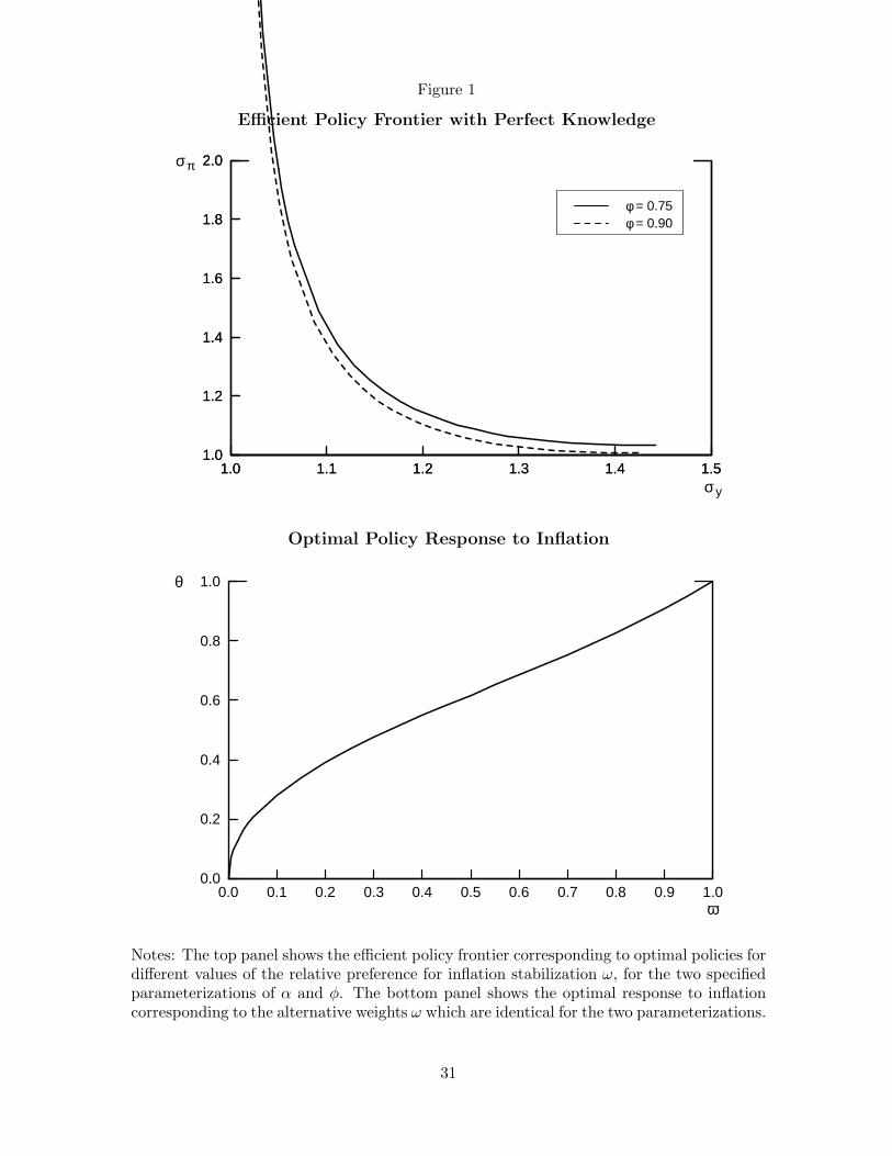
Figure 1

Efficient Policy Frontier with Perfect Knowledge

1.0

1.2

1.4

1.6

1.8

2.0

1.0 1.1 1.2 1.3 1.4 1.5

1.0

1.2

1.4

1.6

1.8

2.0

1.0 1.1 1.2 1.3 1.4 1.5

σ π

σ y

φ = 0.75φ = 0.90

Optimal Policy Response to Inflation

0.0

0.2

0.4

0.6

0.8

1.0

0.0 0.1 0.2 0.3 0.4 0.5 0.6 0.7 0.8 0.9 1.0

θ

ω

Notes: The top panel shows the efficient policy frontier corresponding to optimal policies fordifferent values of the relative preference for inflation stabilization ω, for the two specifiedparameterizations of α and φ. The bottom panel shows the optimal response to inflationcorresponding to the alternative weights ω which are identical for the two parameterizations.

31

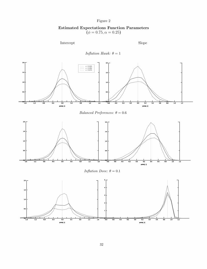
Figure 2

Estimated Expectations Function Parameters(φ = 0.75, α = 0.25)

Intercept Slope

Inflation Hawk: θ = 1

0.0

0.5

1.0

1.5

2.0

-1.6 -1.2 -0.8 -0.4 0.0 0.4 0.8 1.2 1.6

points[, 1]

0.0

0.5

1.0

1.5

2.0

-1.6 -1.2 -0.8 -0.4 0.0 0.4 0.8 1.2 1.6

points[, 1]

0.0

0.5

1.0

1.5

2.0

-1.6 -1.2 -0.8 -0.4 0.0 0.4 0.8 1.2 1.6

points[, 1]

κ = 0.025κ = 0.050κ = 0.075

0.0

0.5

1.0

1.5

2.0

-0.8 -0.6 -0.4 -0.2 0.0 0.2 0.4 0.6 0.8 1.0 1.2

points[, 1]

0.0

0.5

1.0

1.5

2.0

-0.8 -0.6 -0.4 -0.2 0.0 0.2 0.4 0.6 0.8 1.0 1.2

points[, 1]

0.0

0.5

1.0

1.5

2.0

-0.8 -0.6 -0.4 -0.2 0.0 0.2 0.4 0.6 0.8 1.0 1.2

points[, 1]

Balanced Preferences: θ = 0.6

0.0

0.5

1.0

1.5

2.0

-1.6 -1.2 -0.8 -0.4 0.0 0.4 0.8 1.2 1.6

0.0

0.5

1.0

1.5

2.0

-1.6 -1.2 -0.8 -0.4 0.0 0.4 0.8 1.2 1.6

0.0

0.5

1.0

1.5

2.0

-1.6 -1.2 -0.8 -0.4 0.0 0.4 0.8 1.2 1.6

0.0

0.5

1.0

1.5

2.0

-0.8 -0.6 -0.4 -0.2 0.0 0.2 0.4 0.6 0.8 1.0 1.2

points[, 1]

0.0

0.5

1.0

1.5

2.0

-0.8 -0.6 -0.4 -0.2 0.0 0.2 0.4 0.6 0.8 1.0 1.2

points[, 1]

0.0

0.5

1.0

1.5

2.0

-0.8 -0.6 -0.4 -0.2 0.0 0.2 0.4 0.6 0.8 1.0 1.2

points[, 1]

Inflation Dove: θ = 0.1

0.0

0.5

1.0

1.5

2.0

-1.6 -1.2 -0.8 -0.4 0.0 0.4 0.8 1.2 1.6

points[, 1]

0.0

0.5

1.0

1.5

2.0

-1.6 -1.2 -0.8 -0.4 0.0 0.4 0.8 1.2 1.6

points[, 1]

0.0

0.5

1.0

1.5

2.0

-1.6 -1.2 -0.8 -0.4 0.0 0.4 0.8 1.2 1.6

points[, 1]

0

1

2

3

4

5

-0.8 -0.6 -0.4 -0.2 0.0 0.2 0.4 0.6 0.8 1.0 1.2

points[, 1]

0

1

2

3

4

5

-0.8 -0.6 -0.4 -0.2 0.0 0.2 0.4 0.6 0.8 1.0 1.2

points[, 1]

0

1

2

3

4

5

-0.8 -0.6 -0.4 -0.2 0.0 0.2 0.4 0.6 0.8 1.0 1.2

points[, 1]

32

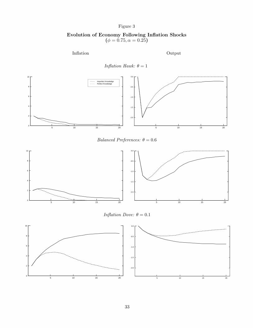
Figure 3

Evolution of Economy Following Inflation Shocks(φ = 0.75, α = 0.25)

Inflation Output

Inflation Hawk: θ = 1

0

2

4

6

8

10

5 10 15 20

Imperfect KnowledgePerfect Knowledge

-2.0

-1.5

-1.0

-0.5

0.0

5 10 15 20

Balanced Preferences: θ = 0.6

0

2

4

6

8

10

5 10 15 20

-2.0

-1.5

-1.0

-0.5

0.0

5 10 15 20

Inflation Dove: θ = 0.1

0

2

4

6

8

10

5 10 15 20

-2.0

-1.5

-1.0

-0.5

0.0

5 10 15 20

33

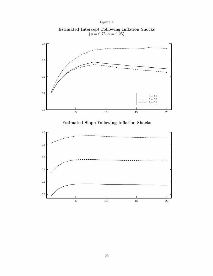
Figure 4

Estimated Intercept Following Inflation Shocks(φ = 0.75, α = 0.25)

0.0

0.1

0.2

0.3

0.4

5 10 15 20

θ = 1.0θ = 0.6θ = 0.1

Estimated Slope Following Inflation Shocks

0.0

0.2

0.4

0.6

0.8

1.0

5 10 15 20

34

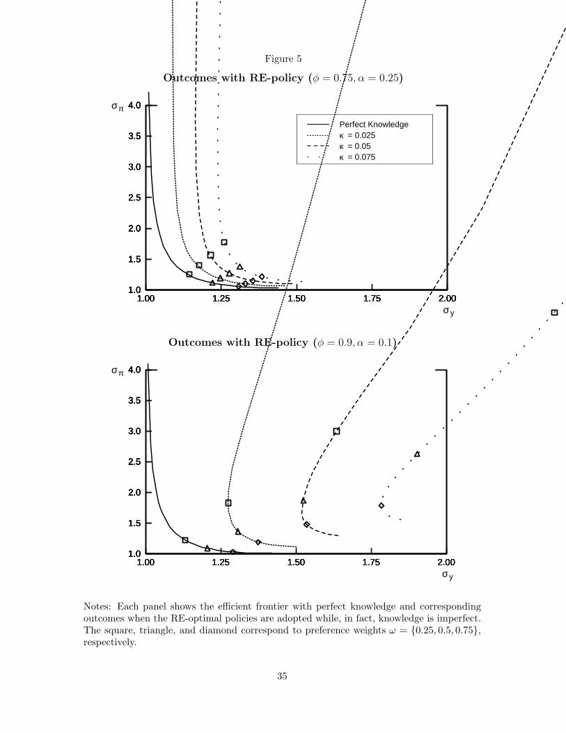
Figure 5

Outcomes with RE-policy (φ = 0.75, α = 0.25)

1.0

1.5

2.0

2.5

3.0

3.5

4.0

1.00 1.25 1.50 1.75 2.00

1.0

1.5

2.0

2.5

3.0

3.5

4.0

1.00 1.25 1.50 1.75 2.00

1.0

1.5

2.0

2.5

3.0

3.5

4.0

1.00 1.25 1.50 1.75 2.00

1.0

1.5

2.0

2.5

3.0

3.5

4.0

1.00 1.25 1.50 1.75 2.00

σ π

σ y

Perfect Knowledgeκ = 0.025κ = 0.05 κ = 0.075

Outcomes with RE-policy (φ = 0.9, α = 0.1)

1.0

1.5

2.0

2.5

3.0

3.5

4.0

1.00 1.25 1.50 1.75 2.00

1.0

1.5

2.0

2.5

3.0

3.5

4.0

1.00 1.25 1.50 1.75 2.00

1.0

1.5

2.0

2.5

3.0

3.5

4.0

1.00 1.25 1.50 1.75 2.00

1.0

1.5

2.0

2.5

3.0

3.5

4.0

1.00 1.25 1.50 1.75 2.00

σ π

σ y

Notes: Each panel shows the efficient frontier with perfect knowledge and correspondingoutcomes when the RE-optimal policies are adopted while, in fact, knowledge is imperfect.The square, triangle, and diamond correspond to preference weights ω = {0.25, 0.5, 0.75},respectively.

35

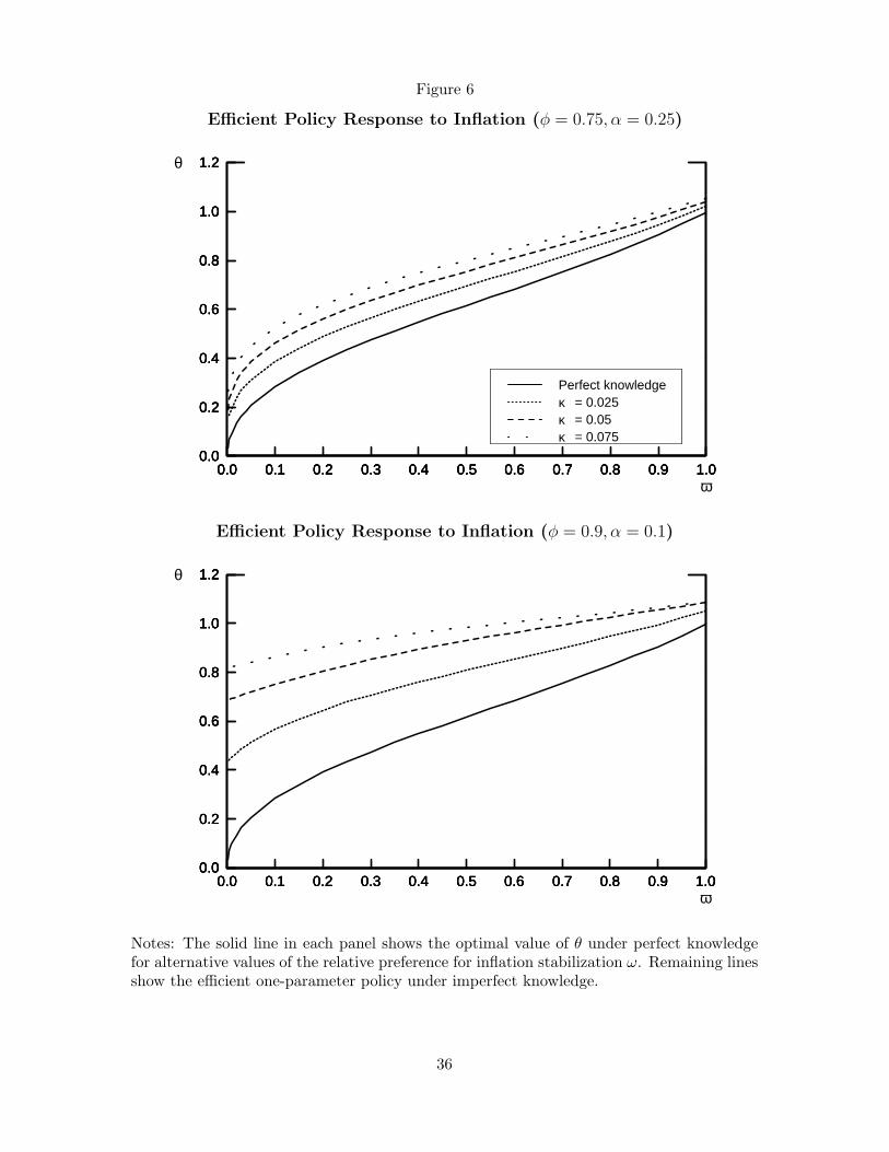
Figure 6

Efficient Policy Response to Inflation (φ = 0.75, α = 0.25)

0.0

0.2

0.4

0.6

0.8

1.0

1.2

0.0 0.1 0.2 0.3 0.4 0.5 0.6 0.7 0.8 0.9 1.0

0.0

0.2

0.4

0.6

0.8

1.0

1.2

0.0 0.1 0.2 0.3 0.4 0.5 0.6 0.7 0.8 0.9 1.0

0.0

0.2

0.4

0.6

0.8

1.0

1.2

0.0 0.1 0.2 0.3 0.4 0.5 0.6 0.7 0.8 0.9 1.0

0.0

0.2

0.4

0.6

0.8

1.0

1.2

0.0 0.1 0.2 0.3 0.4 0.5 0.6 0.7 0.8 0.9 1.0

θ

ω

Perfect knowledgeκ = 0.025κ = 0.05κ = 0.075

Efficient Policy Response to Inflation (φ = 0.9, α = 0.1)

0.0

0.2

0.4

0.6

0.8

1.0

1.2

0.0 0.1 0.2 0.3 0.4 0.5 0.6 0.7 0.8 0.9 1.0

0.0

0.2

0.4

0.6

0.8

1.0

1.2

0.0 0.1 0.2 0.3 0.4 0.5 0.6 0.7 0.8 0.9 1.0

0.0

0.2

0.4

0.6

0.8

1.0

1.2

0.0 0.1 0.2 0.3 0.4 0.5 0.6 0.7 0.8 0.9 1.0

0.0

0.2

0.4

0.6

0.8

1.0

1.2

0.0 0.1 0.2 0.3 0.4 0.5 0.6 0.7 0.8 0.9 1.0

θ

ω

Notes: The solid line in each panel shows the optimal value of θ under perfect knowledgefor alternative values of the relative preference for inflation stabilization ω. Remaining linesshow the efficient one-parameter policy under imperfect knowledge.

36

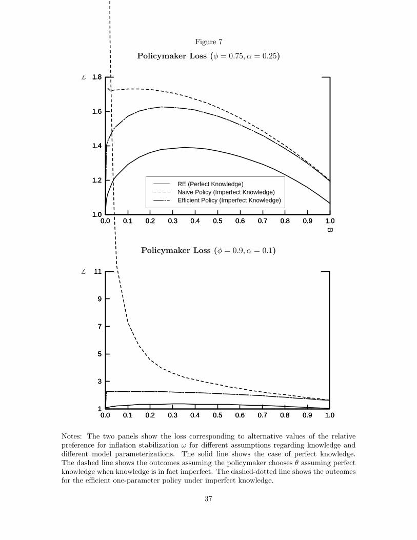
Figure 7

Policymaker Loss (φ = 0.75, α = 0.25)

1.0

1.2

1.4

1.6

1.8

0.0 0.1 0.2 0.3 0.4 0.5 0.6 0.7 0.8 0.9 1.0

1.0

1.2

1.4

1.6

1.8

0.0 0.1 0.2 0.3 0.4 0.5 0.6 0.7 0.8 0.9 1.0

1.0

1.2

1.4

1.6

1.8

0.0 0.1 0.2 0.3 0.4 0.5 0.6 0.7 0.8 0.9 1.0

L

ω

RE (Perfect Knowledge)Naive Policy (Imperfect Knowledge)Efficient Policy (Imperfect Knowledge)

Policymaker Loss (φ = 0.9, α = 0.1)

1

3

5

7

9

11

0.0 0.1 0.2 0.3 0.4 0.5 0.6 0.7 0.8 0.9 1.0

1

3

5

7

9

11

0.0 0.1 0.2 0.3 0.4 0.5 0.6 0.7 0.8 0.9 1.0

1

3

5

7

9

11

0.0 0.1 0.2 0.3 0.4 0.5 0.6 0.7 0.8 0.9 1.0

L

ω

Notes: The two panels show the loss corresponding to alternative values of the relativepreference for inflation stabilization ω for different assumptions regarding knowledge anddifferent model parameterizations. The solid line shows the case of perfect knowledge.The dashed line shows the outcomes assuming the policymaker chooses θ assuming perfectknowledge when knowledge is in fact imperfect. The dashed-dotted line shows the outcomesfor the efficient one-parameter policy under imperfect knowledge.

37

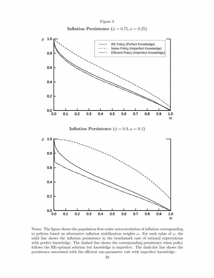
Figure 8

Inflation Persistence (φ = 0.75, α = 0.25)

0.0

0.2

0.4

0.6

0.8

1.0

0.0 0.1 0.2 0.3 0.4 0.5 0.6 0.7 0.8 0.9 1.0

0.0

0.2

0.4

0.6

0.8

1.0

0.0 0.1 0.2 0.3 0.4 0.5 0.6 0.7 0.8 0.9 1.0

0.0

0.2

0.4

0.6

0.8

1.0

0.0 0.1 0.2 0.3 0.4 0.5 0.6 0.7 0.8 0.9 1.0

ρ

ω

RE Policy (Perfect Knowledge)Naive Policy (Imperfect Knowledge)Efficient Policy (Imperfect Knowledge)

Inflation Persistence (φ = 0.9, α = 0.1)

0.0

0.2

0.4

0.6

0.8

1.0

0.0 0.1 0.2 0.3 0.4 0.5 0.6 0.7 0.8 0.9 1.0

0.0

0.2

0.4

0.6

0.8

1.0

0.0 0.1 0.2 0.3 0.4 0.5 0.6 0.7 0.8 0.9 1.0

0.0

0.2

0.4

0.6

0.8

1.0

0.0 0.1 0.2 0.3 0.4 0.5 0.6 0.7 0.8 0.9 1.0

ρ

ω

Notes: The figure shows the population first-order autocorrelation of inflation correspondingto policies based on alternative inflation stabilization weights ω. For each value of ω, thesolid line shows the inflation persistence in the benchmark case of rational expectationswith perfect knowledge. The dashed line shows the corresponding persistence when policyfollows the RE-optimal solution but knowledge is imperfect. The dash-dot line shows thepersistence associated with the efficient one-parameter rule with imperfect knowledge.

38

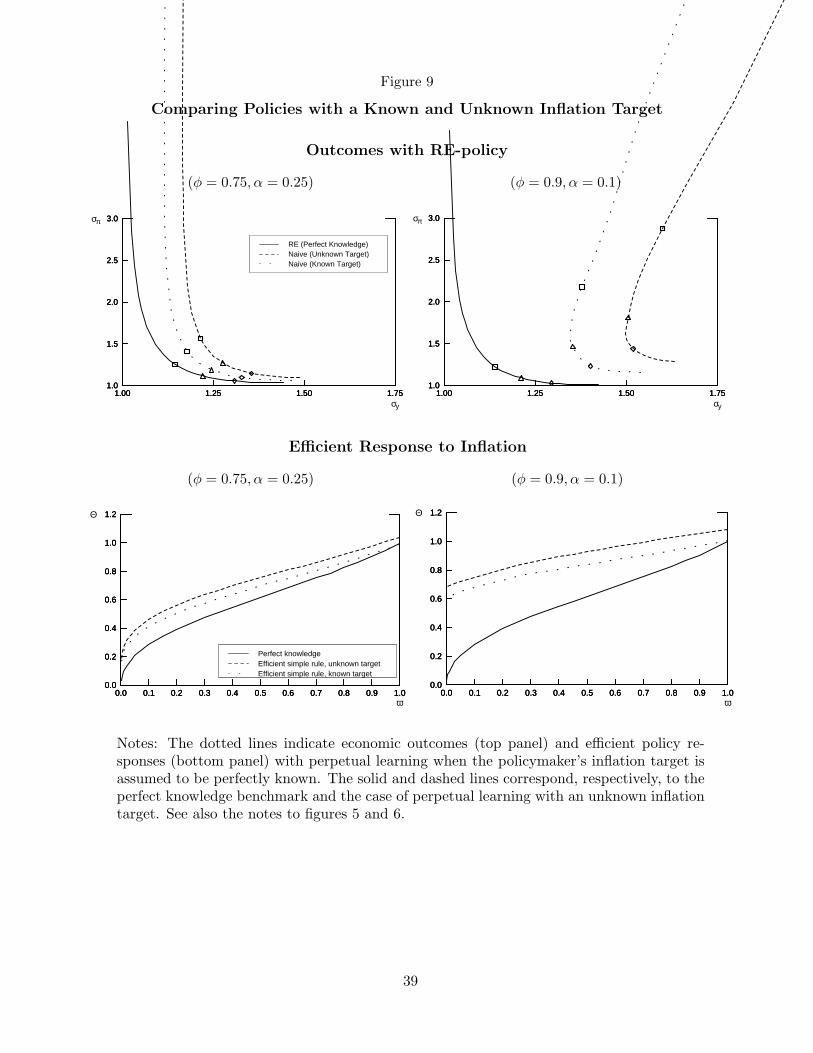
Figure 9

Comparing Policies with a Known and Unknown Inflation Target

Outcomes with RE-policy

(φ = 0.75, α = 0.25) (φ = 0.9, α = 0.1)

1.0

1.5

2.0

2.5

3.0

1.00 1.25 1.50 1.75

1.0

1.5

2.0

2.5

3.0

1.00 1.25 1.50 1.75

1.0

1.5

2.0

2.5

3.0

1.00 1.25 1.50 1.75

σπ

σy

RE (Perfect Knowledge)Naive (Unknown Target)Naive (Known Target)

1.0

1.5

2.0

2.5

3.0

1.00 1.25 1.50 1.75

1.0

1.5

2.0

2.5

3.0

1.00 1.25 1.50 1.75

1.0

1.5

2.0

2.5

3.0

1.00 1.25 1.50 1.75

σπ

σy

Efficient Response to Inflation

(φ = 0.75, α = 0.25) (φ = 0.9, α = 0.1)

0.0

0.2

0.4

0.6

0.8

1.0

1.2

0.0 0.1 0.2 0.3 0.4 0.5 0.6 0.7 0.8 0.9 1.0

0.0

0.2

0.4

0.6

0.8

1.0

1.2

0.0 0.1 0.2 0.3 0.4 0.5 0.6 0.7 0.8 0.9 1.0

0.0

0.2

0.4

0.6

0.8

1.0

1.2

0.0 0.1 0.2 0.3 0.4 0.5 0.6 0.7 0.8 0.9 1.0

Θ

ω

Perfect knowledgeEfficient simple rule, unknown targetEfficient simple rule, known target

0.0

0.2

0.4

0.6

0.8

1.0

1.2

0.0 0.1 0.2 0.3 0.4 0.5 0.6 0.7 0.8 0.9 1.0

0.0

0.2

0.4

0.6

0.8

1.0

1.2

0.0 0.1 0.2 0.3 0.4 0.5 0.6 0.7 0.8 0.9 1.0

0.0

0.2

0.4

0.6

0.8

1.0

1.2

0.0 0.1 0.2 0.3 0.4 0.5 0.6 0.7 0.8 0.9 1.0

Θ

ω

Notes: The dotted lines indicate economic outcomes (top panel) and efficient policy re-sponses (bottom panel) with perpetual learning when the policymaker’s inflation target isassumed to be perfectly known. The solid and dashed lines correspond, respectively, to theperfect knowledge benchmark and the case of perpetual learning with an unknown inflationtarget. See also the notes to figures 5 and 6.

39