NBER WORKING PAPER SERIES

THE BURDEN OF KNOWLEDGE AND THE‘DEATH OF THE RENAISSANCE MAN’:IS INNOVATION GETTING HARDER?

Benjamin F. Jones

Working Paper 11360http://www.nber.org/papers/w11360

NATIONAL BUREAU OF ECONOMIC RESEARCH1050 Massachusetts Avenue

Cambridge, MA 02138May 2005

I wish to thank Pol Antras, Andrei Bremzen, Esther Duflo, Glenn Ellison, Amy Finkelstein, Simon Johnson,Joel Mokyr, Ben Olken, Michael Piore, Scott Stern and participants at various lunches and seminars forhelpful comments. I am especially grateful to Daron Acemoglu, Abhijit Banerjee, and Sendhil Mullainathanfor their advice and Trevor Hallstein for research assistance. The support of the Social Science ResearchCouncil’s Program in Applied Economics, with funding provided by the John D. and Catherine T. MacArthurFoundation, is gratefully acknowledged. The views expressed herein are those of the author(s) and do notnecessarily reflect the views of the National Bureau of Economic Research.

©2005 by Benjamin F. Jones. All rights reserved. Short sections of text, not to exceed two paragraphs, maybe quoted without explicit permission provided that full credit, including © notice, is given to the source.

The Burden of Knowledge and the ‘Death of the Renaissance Man’: Is Innovation Getting Harder?Benjamin F. JonesNBER Working Paper No. 11360May 2005JEL No. O3, O4, J2, I2

ABSTRACT

This paper investigates, theoretically and empirically, a possibly fundamental aspect of technological

progress. If knowledge accumulates as technology progresses, then successive generations of

innovators may face an increasing educational burden. Innovators can compensate in their education

by seeking narrower expertise, but narrowing expertise will reduce their individual capacities, with

implications for the organization of innovative activity - a greater reliance on teamwork - and

negative implications for growth. I develop a formal model of this "knowledge burden mechanism"

and derive six testable predictions for innovators. Over time, educational attainment will rise while

increased specialization and teamwork follow from a sufficiently rapid increase in the burden of

knowledge. In cross-section, the model predicts that specialization and teamwork will be greater in

deeper areas of knowledge while, surprisingly, educational attainment will not vary across fields. I

test these six predictions using a micro-data set of individual inventors and find evidence consistent

with each prediction. The model thus provides a parsimonious explanation for a range of empirical

patterns of inventive activity. Upward trends in academic collaboration and lengthening doctorates,

which have been noted in other research, can also be explained by the model, as can much-debated

trends relating productivity growth and patent output to aggregate inventive effort. The knowledge

burden mechanism suggests that the nature of innovation is changing, with negative implications for

long-run economic growth.

Benjamin F. JonesNorthwestern UniversityKellogg School of ManagementDepartment of Management and Strategy2001 Sheridan RoadEvanston, IL 60208and NBERbjones@kellogg.northwesterm.edu

1 Introduction

Understanding innovation is central to understanding many important aspects of economics,

from market structure to aggregate growth. Innovators, in turn, are a necessary input to

any innovation. The innovator, wrestling with a creative idea, working with colleagues,

bringing an idea to fruition, seems the very heart of the innovative process.

This paper places innovators at the center of analysis and focuses on two simple observa-

tions. First, innovators are not born at the frontier of knowledge; rather, they must initially

undertake significant education. Second, the frontier of knowledge shifts over time. The

purpose of this paper is to investigate equilibrium implications of these two observations

and then test these implications empirically. The theory and empirical work below suggest

possibly fundamental consequences for the organization of innovative activity and, in the

aggregate, for growth.

The first observation concerns human capital and highlights a general distinction be-

tween human capital and other stock variables. Physical stocks can be transferred easily, as

property rights, from one agent to another. Human capital, by contrast, is not transferred

easily. While one generation may rather effortlessly bequeath its physical assets to the next,

with human capital stocks, this is fundamentally not the case. The vessel of human cap-

ital - the individual - absorbs information at a limited rate, has limited capacity, and has

limited time on earth. The difficulty of transferring human capital has broad implications

in economics1; in this paper, I focus on basic implications for innovation.

The second observation concerns the total stock of knowledge. In 1676, Isaac Newton

wrote famously to Robert Hooke, “If I have seen further it is by standing on the shoulders

of giants.” Newton’s sentiment suggests that knowledge begets new knowledge, an observa-

tion that has been formalized in the growth literature (Romer 1990, Jones 1995a, Weitzman

1998) with implications discussed extensively both there (e.g. Jones 1995b, Kortum 1997,

Young 1998) and in the micro-innovation literature (e.g. Scotchmer 1991, Henderson &

Cockburn 1996). This paper suggests a different, indirect implication of Newton’s obser-

vation: if one is to stand on the shoulders of giants, one must first climb up their backs,

and the greater the body of knowledge, the harder this climb becomes.

1See, for example, Ben-Porath (1967) regarding life-cyle earnings and Hart & Moore (1995) regardingdebt contracts.

1

If technological progress leads to an accumulation of knowledge, then the educational

burden on successive cohorts of innovators will increase. Innovators might confront this

difficulty by choosing to learn more. Alternatively, they might compensate by choosing

narrower expertise — a "death of the Renaissance Man" effect. Choosing to learn more will

leave less time in the life-cycle for innovation. Narrowing expertise, meanwhile, can reduce

individual capabilities and force innovators to work in teams. Intriguing evidence along the

lines of a "learning more" effect can be seen in Table 1, which borrows from Jones (2005).

We see that the mean age at which great inventors and Nobel Prize winners produced their

great innovations increased by 6 years over the course of the 20th Century. To help motivate

the second set of effects, consider the invention of the microprocessor. As described by

Malone (1995), the invention was by necessity the work of a team. The inspiration began

with a researcher named Ted Hoff, who joined in the theoretical development with Stan

Mazor. But as Malone writes,

Hoff and Mazor didn’t really know how to translate this architecture into a

working chip design... The project began to lag.

In fact, probably only one person in the world did know how to do the next

step. That was Federico Faggin...

The microprocessor was one person’s inspiration, but several people’s invention. It is the

story of researchers with circumscribed abilities, working in a team, and it helps motivate

the model of innovation and the empirical work in this paper.

In the model, presented in Section 2, innovators are specialists who interact with each

other in the implementation of their ideas. The model introduces a "circle of knowledge" — a

continuum of types of knowledge — upon which innovators define their specialties and locate

necessary teammates. Achieving expertise in any area on the circle requires an innovator

to bring herself to the frontier of knowledge in that area, and the difficulty of reaching the

frontier — the burden of knowledge — may increase or decrease over time.

The central choice problem is that of career. At birth, each individual chooses to become

either a production worker or an innovator. Innovators must further choose a specific area

of knowledge to learn. They choose their degree of specialization as a tradeoff between the

costs and benefits of education: greater knowledge leads to increased innovative potential,

but it also costs more to acquire. Innovators also seek to avoid crowding: other things equal,

2

the greater the density of innovators in a particular area of knowledge, the less expected

income each will earn. The equilibrium defines the educational decisions of innovators — the

total amount of education they seek, their degree of specialization, and their consequent

propensity to form teams.

Career choices are made in a dynamically evolving economy. The model marries the

burden of knowledge mechanism with two established insights in the growth and innovation

literatures. First, a growing population increases market size, making innovations more

valuable and attracting workers to the innovative sector. The importance of introducing

such scale effects from an aggregate growth perspective was first pointed out by Jones

(1995a). In this model, increasing market size also plays a key role by increasing the

marginal value of education, thereby increasing the amount of education innovators wish

to seek. Second, the value of knowledge may be increasing or decreasing as the economy

evolves. This feature captures, in reduced-form, a broad range of arguments in the literature:

both fishing-out ideas (e.g. Kortum 1997), as well as more optimistic specifications where

knowledge is increasingly useful (e.g. Romer 1990, Aghion & Howitt 1992). An increasing

value of knowledge will tend, ceteris paribus, to increase the marginal benefit of education.

Finally, the difficulty in reaching the knowledge frontier — the burden of knowledge — may

rise or fall as the economy evolves.

In this framework the same forces that influence innovators’ educational decisions also

influence long-run growth. Indeed, the tight link between individual income possibilities

and changes in the knowledge space produces detailed predictions about innovator behavior

on the one hand and aggregate consequences on the other, allowing this model to explain

both micro and aggregate data patterns. The crux of the model is that income possibili-

ties determine career decisions. Therefore, any increase in the burden of knowledge cannot

be analyzed in isolation but must be weighed against both the value of this knowledge

and other income opportunities when innovators make their career choices. Moreover, any

simple intuition that areas of "greater knowledge" require more education and/or more

specialization turns out to have important and empirically relevant qualifications. Along

the balanced growth path, the income possibilities of innovation expand — because market

size and/or the value of ideas are increasing — so that new cohorts will seek more educa-

tion over time. Given this increasing educational attainment, innovators will only become

more specialized if the burden of knowledge mechanism is sufficiently strong. More subtly,

3

income arbitrage produces the surprising result that educational attainment will not vary

across technological fields, regardless of variation in the burden of knowledge or innovative

opportunities.

In all, the model makes six testable predictions for the behavior of individual innovators.

In time series, the model predicts that (i) educational attainment will be rising while (ii)

specialization and (iii) teamwork will increase only if the burden of knowledge is increasing

at a sufficient rate. In cross-section, the model predicts that (iv) specialization and hence

(v) teamwork will be greater in fields where knowledge is deeper. At the same time, (vi)

educational attainment should show no variation across technological fields.

Section 3 tests these six predictions empirically. Using a rich patent data set (Hall et

al. 2001) together with the results of a new data collection exercise to determine the ages

of 55,000 inventors, I am able to develop detailed patent histories for individuals. As shown

in Figure 1, I find that the age at first innovation, which can serve as a proxy measure for

educational attainment, is trending upwards at 0.6 years per decade. Meanwhile, U.S. team

size is seen to be increasing at a remarkably steep rate of 17% per decade, and a direct

measure for specialization is increasing by 6% per decade. As discussed in Section 3, these

trends are all robust to a number of controls, and in particular are robust across a wide

range of technological categories and research environments.

In cross-section, I find striking support for the model’s perhaps less obvious prediction

that educational attainment will be similar across fields. At the same time, team size and

the specialization measure vary substantially across fields, and, as predicted, are larger

where the amount of knowledge underlying each patent is larger.

The model thus serves as a parsimonious explanation for this collection of new facts.

Starting with simple observations about human capital and knowledge, we are led to test

basic predictions about innovator behavior and to uncover substantial variations across

fields and over time. As discussed in Section 4, the model can further explain several facts

that have been documented elsewhere, including upward trends in academic coauthorship

and doctoral duration. Lastly, in the aggregate, the model provides one consistent expla-

nation for existing facts debated by growth economists. First, R&D employment in leading

economies has been rising dramatically, yet TFP growth has been flat (Jones, 1995b). Sec-

ond, the average number of patents produced per R&D worker or R&D dollar has been

falling over time across countries (Evenson 1984) and U.S. manufacturing industries (Kor-

4

tum 1993). These aggregate data trends can be seen in the model as an effect of increasingly

narrow expertise, where innovators are becoming less productive as individuals and are re-

quired to work in ever larger teams.

Section 4 reviews the results, connects them to existing literatures, and further discusses

their implications.

2 The Model

The over-arching theme of this model is the emphasis on innovators. I analyze a simple struc-

ture with two sectors: a production sector where competitive firms produce a homogenous

output good and an innovation sector where innovators produce productivity-enhancing

ideas. Workers in the production sector earn a competitive wage while innovators earn

income by licensing their ideas to firms in the production sector. I abstract from physical

capital and focus on the role of human capital in the innovation sector. Innovators must

undertake a costly human capital investment to bring themselves to the knowledge frontier

where they become able to innovate. Innovators face a tradeoff between the costs of seeking

more education and the benefits of achieving a broader degree of expertise. This tradeoff

will be balanced differently by different cohorts as the economy evolves.

Section 2.1 describes the production sector and Section 2.2 defines individuals’ life-

cycles and preferences. Sections 2.3 and 2.4 focus on innovators. The first describes the

knowledge space and the cost of education. The second considers the innovation process

and the value of ideas. Section 2.5 defines individuals’ equilibrium choices. Section 2.6

analyzes steady-state growth, and Section 2.7 examines the time-series predictions of the

model. Section 2.8 extends the model to investigate its predictions across technological

areas at a point in time. The predictions of Sections 2.7 and 2.8 are the foundation for the

empirical analysis in Section 3.

2.1 The Production Sector

Competitive firms in the production sector produce a homogenous output good. A firm j

hires an amount of labor, lj(t), to produce output, yj(t) = Xj(t)lj(t). The productivity

level of firm j isXj(t) ≤ X(t), whereX(t) is the leading edge of productivity in the economy,

which can be achieved by any firm with access to the entire set of productive ideas.

5

The firm pays workers a wage, w(t), and makes royalty payments per worker of r(t)

on any patented technologies it employs. While patent protection lasts, the monopolist

innovator will charge a firm a fee, per period, equivalent to all the extra output the firm can

produce with the innovation, and the firm will be just willing to pay this fee. Therefore

Xj(t) = X(t) ∀j, and the total output in the economy is:

Y (t) = X(t)LY (t) (1)

The revenues of these competitive firms are dispensed entirely in wage and royalty payments,

X(t)lj(t) = w(t)lj(t) + r(t)lj(t). The competitive wage paid to a production worker is

therefore:

w(t) = X(t)− r(t) (2)

2.2 Workers and Preferences

There is a continuum of workers of measure L(t) in the economy at time t. This population

grows at rate gL. Individuals are risk neutral and face a constant hazard rate φ of death.

They share a common intertemporal utility function,2

U(τ) =

Z ∞

τc(t)e−φ(t−τ)dt (3)

I assume that individuals are born without assets and supply a unit of labor inelastically

at all points over their lifetime. From the standard intertemporal budget constraint, the

individual’s utility is equivalent to the present value of her expected lifetime non-interest

income.

The choice problem is that of career. At birth, an individual decides whether to become

a wage worker or an innovator. Wage workers require no education and their expected

utility is simply the discounted flow of the wage payments they receive:

Uwage (τ) =

Z ∞

τw(t)e−φ(t−τ)dt (4)

If an individual i chooses to be an innovator instead, then she must further choose a

specific field of expertise and pay an immediate fixed cost of education, E, to bring herself2For simplicity of exposition, I will specify the incomes and expenditures in the model in terms of a

unit-mass of individuals.

6

to the frontier of knowledge in that area. Having paid this cost, the innovator earns

an expected flow of income, v, by licensing any innovations she produces to firms in the

production sector. In the model, both v and E are specific to the choice of expertise made

by an individual (i). The educational cost will also depend on the state of knowledge at the

time of birth (τ), and income flows will further depend on the current state of the economy

(t). The expected lifetime utility of an innovator is written generally as,

UR&Di (τ) =

Z ∞

τvi(t)e

−φ(t−τ)dt−Ei(τ) (5)

The structure of the innovator’s educational choice and the functional forms of v and E are

the subject of the next two subsections.

Note that an extended model can further allow for educational time, so that education

has an opportunity cost (foregone income) in addition to any out-of-pocket cost. The

simpler model presented here provides the same themes as the extended model, so this

paper will feature the simpler case; the extended model is provided in the Appendix.

2.3 Knowledge and Education

A type of knowledge is defined by its position, s, on the unit circle. For example, one

segment of the circle might represent electronics, another biochemistry, another economics.

At a point in time, the amount of knowledge at each point on the circle is assumed to be

the same.3 I define this quantity as D(t).

The prospective innovator chooses an area of expertise: a point, si, on the circle and

a certain distance, bi ∈ [0, 1], to its right. For an innovator born at time τ , the amount ofknowledge the innovator acquires is the chosen breadth of expertise, bi, multiplied by the

prevailing depth of knowledge, D(τ). The educational cost of acquiring this information

is:

Ei(τ) = (biD(τ))ε (6)

where ε > 0, which says only that learning more requires a greater amount of education. I

make no a priori assumption about whether education costs are convex or concave in the

amount of information the innovator learns.3 I will partly relax this assumption when I consider a cross-sectional variation of the model in Section

2.8.

7

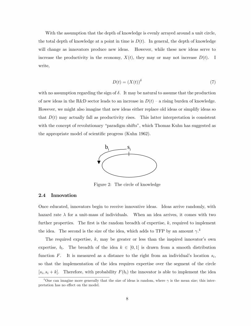
With the assumption that the depth of knowledge is evenly arrayed around a unit circle,

the total depth of knowledge at a point in time is D(t). In general, the depth of knowledge

will change as innovators produce new ideas. However, while these new ideas serve to

increase the productivity in the economy, X(t), they may or may not increase D(t). I

write,

D(t) = (X(t))δ (7)

with no assumption regarding the sign of δ. It may be natural to assume that the production

of new ideas in the R&D sector leads to an increase in D(t) — a rising burden of knowledge.

However, we might also imagine that new ideas either replace old ideas or simplify ideas so

that D(t) may actually fall as productivity rises. This latter interpretation is consistent

with the concept of revolutionary “paradigm shifts”, which Thomas Kuhn has suggested as

the appropriate model of scientific progress (Kuhn 1962).

sibi

Figure 2: The circle of knowledge

2.4 Innovation

Once educated, innovators begin to receive innovative ideas. Ideas arrive randomly, with

hazard rate λ for a unit-mass of individuals. When an idea arrives, it comes with two

further properties. The first is the random breadth of expertise, k, required to implement

the idea. The second is the size of the idea, which adds to TFP by an amount γ.4

The required expertise, k, may be greater or less than the inspired innovator’s own

expertise, bi. The breadth of the idea k ∈ [0, 1] is drawn from a smooth distribution

function F . It is measured as a distance to the right from an individual’s location si,

so that the implementation of the idea requires expertise over the segment of the circle

[si, si + k]. Therefore, with probability F (bi) the innovator is able to implement the idea

4One can imagine more generally that the size of ideas is random, where γ is the mean size; this inter-pretation has no effect on the model.

8

alone, and with probability 1− F (bi) the innovator needs at least one partner. That is, I

allow for the formation of teams.

I assume that the innovator with the idea acts as a monopolist vis-a-vis potential team-

mates so that, by Bertrand reasoning, the inspired innovator receives all profits from the

project. I further assume that once an idea arrives it can be implemented instantaneously

and without any expenditure (in particular, team formation is costless). Therefore, (i) all

projects are profitable, (ii) the inspired, monopolist innovator will receive the entire royalty

stream from the project as personal income, and (iii) any necessary teammates will be just

willing to help without compensation.5

I make two further assumptions regarding team formation. The inspired innovator will

choose team members from her own cohort if possible and assemble the minimum number

of people necessary to implement the idea. These assumptions are innocuous and are made

to permit explicit analysis of average team size in Sections 2.7 and 2.8.

Given that an idea can be licensed for use by LY workers, and patent protection lasts

for z years, the market size for a patent is:

M(t) =

Z t+z

tLY (et)det (8)

and the lump-sum value of the patent is therefore V (t) = γM(t).6

The expected flow of income to an innovator is v = λV , the probability of having an

idea at a point in time times the income the idea generates. Using the definition of V , we

can write v = λγM . The expected flow of income is therefore equivalently understood as

the expected rate at which the innovator adds to TFP, λγ, times the market size for the

innovation. When considering the time lag between an innovator’s innovations, it will be

useful to consider λ and γ separately. However, in determining equilibrium choices, I wish

to emphasize that the combination of these parameters is the important primitive. I will

5The only possible obstacle to implementation is an absence of required expertise. Anticipating theequilibrium of this model, innovators’ collective expertise will cover the entire circle of knowledge, so thatall ideas are feasible and therefore all ideas will in fact be implemented. To avoid burdensome notation inthe text, I will write the rest of the model assuming this result. The Appendix considers the general caseand establishes this result as part of any (subgame perfect) equilibrium.

6This expression is written assuming the innovator has access to a competitive financial market which willpay the innovator the lump-sum value of the patent (or an equivalent annuity) in exchange for the patentrights. If no such market were available, the value of the patent to the innovator would need to reflect thepossibility that the innovator dies before the patent rights expire, in which case V = γ

t+z

tLY (t)e

−φ(t−t)dt.This variation will have no impact on the main results of the model.

9

therefore define θ = λγ as a summary measure of innovator productivity and, for brevity,

proceed in defining the final pieces of the model on the basis of θ.

Specifically, I assume that innovator productivity will depend on three things: (1) the

level of technology; (2) the current degree of competition in the innovator’s specialty; and

(3) the innovator’s breadth of expertise. In particular, I write,

θi(t) = X(t)χL(t, si)−σbβi (9)

where X(t) is the productivity level in the economy, L(t, si) is the mass of individuals at

time t who share the innovator’s specialty, and bi is the innovator’s breadth of expertise.

These reduced-form specifications capture several key ideas. The parameter χ represents

the impact of the state of technology on an innovator’s productivity. It incorporates

the standard ideas in the literature which were alluded to in the introduction: “fishing-

out” hypotheses whereby innovators’ productivity falls as the state of knowledge advances

(χ < 0), and “positive intertemporal spillovers” whereby an improving state of knowledge

makes innovators more productive (χ > 0).7

The parameter σ represents the impact of crowding on the frequency of an innovator’s

ideas. I assume σ > 0, following standard arguments where innovators partly duplicate

each other’s work. A greater density of workers in the same specialty increases duplication,

reducing the rate at which a specific individual produces a novel idea.

The final parameter, β, represents the impact of the breadth of expertise. A specification

with β > 0 suggests simply that greater human capital increases one’s productivity. The

specific reason I embrace, for the purposes of this model, is that individuals with broader

expertise access a larger set of available knowledge — facts, theories, methods — on which to

build innovations. This will increase their innovative abilities, along the lines of Weitzman

(1998), making them more productive.8

7Note that I am using the state variable X(t) to represent the effect of both technology and the stateof knowledge on an innovator’s capabilities. Adding a separate channel to differentiate between “ideas”and “technology” will add little insight. When I discuss cross-sectional predictions in Section 2.8, whereit will be useful to think of different knowledge levels across technological areas, I will introduce a richerspecification.

8There are many other mechanisms through which broader expertise would enhance an innovator’s in-come. First, a more broadly expert innovator may better evaluate the expected impact and feasibility ofher ideas. She will better select toward high value, successful lines of inquiry, and therefore achieve greaterreturns. Second, if assembling teams is costly, innovators will be unwilling to form large teams. Morebroadly expert innovators can rely less on large teams for the implementation of their ideas, making theirideas less costly to implement. Third, if income is shared across team members, then broader expertise,

10

Finally, I can now explicitly define an innovator’s expected flow of income,

vi(t) = X(t)χL(t, si)−σbβi M(t) (10)

2.5 Equilibrium Choices

The choice facing each individual is that of career, which is a one-shot decision made at

birth. Define the set of individuals born at time τ as l(τ), of which a subset lY (τ) choose

the production sector and a subset lR(τ) choose the innovation sector instead. Those

who choose the innovation sector must additionally choose an area of expertise (s, b). In

equilibrium, we require two conditions for each cohort τ :

UR&Di (si, bi) ≥ UR&D

i (s, b) ∀s, b ∀i ∈ lR(τ) (11)

UR&Di (τ) = Uwage (τ) = U∗ (τ) ∀i ∈ lR(τ) ∀j ∈ lY (τ) (12)

The first condition states that no innovator can deviate to any other educational choice and

be better off. The second condition rules out income arbitrage possibilities between the

R&D and production sectors. With the definitions of the model in Sections 2.1 through

2.4, we can now define the expected income from various choices and hence, with conditions

(11) and (12), the equilibrium outcome.

2.5.1 Production workers

Production workers receive a competitive wage w(t) = X(t)− r(t), as defined in (2). Since

patents are protected for z years, the flow of royalty payments r(t) is simply X(t)−X(t−z)and therefore w(t) = X(t− z). In other words, the wage earned by a production worker is

that portion of productivity which is not patent-protected, which is just the productivity

level of the economy z years previously.

Choosing to be a production worker therefore provides lifetime income of

U∗ (τ) =Z ∞

τX(t− z)e−φ(t−τ)dt (13)

which reduces the necessary team size, will bring one a greater share of project income. These last twoeffects will lead more narrowly expert innovators to abandon a greater portion of their broad ideas.

11

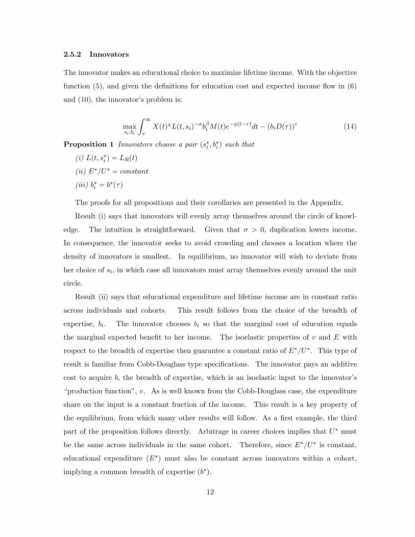
2.5.2 Innovators

The innovator makes an educational choice to maximize lifetime income. With the objective

function (5), and given the definitions for education cost and expected income flow in (6)

and (10), the innovator’s problem is:

maxsi,bi

Z ∞

τX(t)χL(t, si)

−σbβi M(t)e−φ(t−τ)dt− (biD(τ))ε (14)

Proposition 1 Innovators choose a pair (s∗i , b∗i ) such that

(i) L(t, s∗i ) = LR(t)

(ii) E∗/U∗ = constant

(iii) b∗i = b∗(τ)

The proofs for all propositions and their corollaries are presented in the Appendix.

Result (i) says that innovators will evenly array themselves around the circle of knowl-

edge. The intuition is straightforward. Given that σ > 0, duplication lowers income.

In consequence, the innovator seeks to avoid crowding and chooses a location where the

density of innovators is smallest. In equilibrium, no innovator will wish to deviate from

her choice of si, in which case all innovators must array themselves evenly around the unit

circle.

Result (ii) says that educational expenditure and lifetime income are in constant ratio

across individuals and cohorts. This result follows from the choice of the breadth of

expertise, bi. The innovator chooses bi so that the marginal cost of education equals

the marginal expected benefit to her income. The isoelastic properties of v and E with

respect to the breadth of expertise then guarantee a constant ratio of E∗/U∗. This type of

result is familiar from Cobb-Douglass type specifications. The innovator pays an additive

cost to acquire b, the breadth of expertise, which is an isoelastic input to the innovator’s

“production function”, v. As is well known from the Cobb-Douglass case, the expenditure

share on the input is a constant fraction of the income. This result is a key property of

the equilibrium, from which many other results will follow. As a first example, the third

part of the proposition follows directly. Arbitrage in career choices implies that U∗ must

be the same across individuals in the same cohort. Therefore, since E∗/U∗ is constant,

educational expenditure (E∗) must also be constant across innovators within a cohort,

implying a common breadth of expertise (b∗).

12

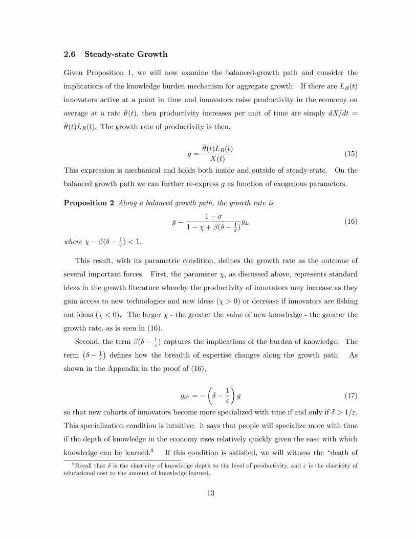
2.6 Steady-state Growth

Given Proposition 1, we will now examine the balanced-growth path and consider the

implications of the knowledge burden mechanism for aggregate growth. If there are LR(t)

innovators active at a point in time and innovators raise productivity in the economy on

average at a rate_θ(t), then productivity increases per unit of time are simply dX/dt =

_θ(t)LR(t). The growth rate of productivity is then,

g =

_θ(t)LR(t)

X(t)(15)

This expression is mechanical and holds both inside and outside of steady-state. On the

balanced growth path we can further re-express g as function of exogenous parameters.

Proposition 2 Along a balanced growth path, the growth rate is

g =1− σ

1− χ+ β(δ − 1ε )gL (16)

where χ− β(δ − 1ε ) < 1.

This result, with its parametric condition, defines the growth rate as the outcome of

several important forces. First, the parameter χ, as discussed above, represents standard

ideas in the growth literature whereby the productivity of innovators may increase as they

gain access to new technologies and new ideas (χ > 0) or decrease if innovators are fishing

out ideas (χ < 0). The larger χ - the greater the value of new knowledge - the greater the

growth rate, as is seen in (16).

Second, the term β(δ − 1ε ) captures the implications of the burden of knowledge. The

term¡δ − 1

ε

¢defines how the breadth of expertise changes along the growth path. As

shown in the Appendix in the proof of (16),

gb∗ = −µδ − 1

ε

¶g (17)

so that new cohorts of innovators become more specialized with time if and only if δ > 1/ε.

This specialization condition is intuitive: it says that people will specialize more with time

if the depth of knowledge in the economy rises relatively quickly given the ease with which

knowledge can be learned.9 If this condition is satisfied, we will witness the “death of9Recall that δ is the elasticity of knowledge depth to the level of productivity, and ε is the elasticity of

educational cost to the amount of knowledge learned.

13

the Renaissance Man” along the growth path (gb∗ < 0). The impact of specialization on

growth will be large or small depending on the value of β, which defines the sensitivity of

innovators’ productivity to their breadth of expertise.10

Expression (16) also shows that growth in per-capita income depends on population

growth, gL. This is the standard Jones (1995b) style result, where increasing effort is

needed to produce steady-state growth. A growing population provides both the motive —

increasing market size — and the means - more minds - for innovative effort to grow at an

exponential rate, even if innovation is getting harder. The alternative, Romer (1990) style

result, where growth can be sustained with constant effort, is obtained in the knife-edge case

where χ− β(δ − 1ε ) = 1.

11 The burden of knowledge mechanism (captured by β(δ − 1ε )) is

therefore felt either by (i) pushing us toward a world where ever-increasing effort is needed

to sustain steady growth or (ii) producing lower growth rates given that we are already in

that world.

Essentially, the greater the growth in the burden of knowledge, the greater must be the

growth in the value of knowledge to compensate. Articulated views of why innovation may

be getting harder in the growth literature (Kortum 1997, Segerstrom 1998) have focused on a

"fishing out" idea; that is, on the parameter χ. The innovation literature also tends to focus

on "fishing out" themes (e.g. Evenson 1991, Cockburn & Henderson, 1996). This paper

offers the burden of knowledge as an alternative mechanism, one that makes innovation

harder, acts similarly on the growth rate, and can explain aggregate data trends (see Section

4). Most importantly, the model makes specific predictions about the behavior of individual

innovators, allowing one to get underneath the aggregate facts and test for a possible rising

burden of knowledge using micro-data. These predictions are defined in the next two

sub-sections.

2.7 Time Series Predictions

Given the equilibrium properties defined in Proposition 1, we can derive three features of

innovator behavior over time.10 In a model with a time cost for education, an increasing burden of knowledge is also felt through increased

educational time, as this reduces the portion of the life-cycle left over to actively pursue innovations. TheAppendix considers this more general model.11Of course, if χ+ β( 1ε − δ) = 1 then growth will explode if gL > 0 (see (16)). This "scale effect" makes

this knife-edge case inconsistent with aggregate data patterns, a problem discussed in detail elsewhere (Jones1995b; Jones 1999).

14

Corollary 1 Along the balanced growth path

(i) gE∗ = g

(ii) gb∗ < 0 iff δ > 1/ε

(iii) team(t) > 0 iff δ > 1/ε

The first result says that educational attainment of successive cohorts increases along

the growth path. Since the value of education to innovators is complementary to growing

income possibilities — due to increasing market size if nothing else — innovator cohorts will

seek more education over time. In equilibrium the optimal amount of education is a fixed

fraction of the innovator’s lifetime income — see Proposition 1. As the economy grows,

individual incomes grow at rate g. In consequence, the amount of education innovators

seek also grows at rate g.12

Note that increasing educational attainment is not driven in equilibrium by an increasing

educational burden: rather, it is driven by the expanding benefits that education affords.

Along the growth path, educational attainment will rise regardless of whether the distance

to the frontier is increasing.

This equilibrium property provides further intuition for the second result, regarding

specialization, which was discussed in the prior section. Increasing educational attainment

implies that δ > 1/ε, rather than δ > 0, is required for expertise to narrow along the growth

path. That is, given increasing educational attainment, the knowledge stock must not only

grow, but grow at a sufficiently high rate to result in narrowing expertise. The third result,

the behavior of average team size, team(t), follows the same condition as specialization.

This result should seem intuitive: more specialized workers rely more on teamwork for the

implementation of their ideas.13

2.8 Cross-sectional Predictions

In this section I extend the model to consider variations across technological areas. The

extension considers J unit circles of knowledge in place of a single circle. I assume that12The extended model in the Appendix gives this result an explicit "time" interpretation, showing that

the duration of education is increasing along the growth path.13An interesting extension considers the possibility that more narrowly educated individuals might have

a narrower range of inspiration (smaller average k). I explore this extension formally in the Appendix andderive there a generalized condition for team size to increase as specialization increases. The intuition,which is shown clearly for a uniform distribution, is that team size will increase with specialization as longas the “reach” of innovators (the breadth of their creativity) does not decline as rapidly as their “grasp”(the breadth of their personal expertise).

15

the elasticity parameters are the same across all areas of knowledge, while each circle has a

specific depth of knowledge Dj and a separate parameter Aj , which represents the relative

productivity of knowledge in that area — whether the area is hot or cold. The structure

of the model is as before, with two modifications. First, the difficulty of reaching the

knowledge frontier will differ across technological areas. The educational cost for each area

j is:

Eij(τ) = (bijDj(τ))ε (18)

Second, an innovator’s productivity will depend on the characteristics of the technological

area. I redefine θ as

θij(t) = Aj(t)X(t)χLj(t, sij)

−σbβij (19)

This specification differs in two ways from that in equation (9). First, the congestion

effects are now specific to the particular technological area, which is indicated by adding

the subscript j to L(t, si). Second, I add the new parameter, Aj(t), to indicate sector

specific research opportunities. Innovators’ inspirations are drawn from a distribution

Fj [sij , sij + 1], so that all ideas from an innovator operating in area j are implementable

using expertise within that circle of knowledge.

The innovator’s maximization problem is solved just as in Section 2.5, only we now

consider the choice problem within a particular area of knowledge j. This generalized

model results in a simple generalization of Proposition 1.

Proposition 3 Innovators choose a pair (sij , bij) and a circle j such that

(i) Lj(t, sij) = Lj(t)

(ii) E∗/U∗ = constant

(iii) b∗ij(τ) = b∗j (τ)

The results of Proposition 3 follow the same logic as Proposition 1. Innovators spread

out to avoid duplicating each other. They choose their breadth of expertise such that

educational expenditure and lifetime income are in constant ratio. Result (iii) and the

central cross-sectional implications follow directly from this latter property.

16

Corollary 2 The equilibrium implies that for any cohort τ

(i) E∗ij(τ) = E∗(τ) ∀i, j(ii) b∗j (τ) < b∗j0(τ) iff Dj(τ) > Dj0(τ)

(iii) teamj (τ) > teamj0 (τ) iff Dj(τ) > Dj0(τ)

The first result says that innovators will choose the same amount of education across

sectors, regardless of differences in the depth of knowledge or innovation opportunities.

This result is perhaps surprising, but the intuition is straightforward. Innovators allocate

themselves across sectors so that differences in the degree of congestion will offset the

variation in technological opportunities or educational burden. Once income is equated

across sectors, innovators acquire the same total education because their optimal amount

of education is a constant fraction of their expected income. The model thus makes the

interesting dual prediction that successive cohorts of innovators will choose an increasing

amount of education, while a given innovator cohort will choose an identical amount of

education across widely different sectors.

In contrast, while we expect no variation in the level of education across sectors, we do

expect differences in specialization and teamwork. Given that total educational attainment

will be the same across sectors, those sectors with deeper knowledge must consequently see

narrower expertise (Corollary 2.ii). In consequence, team size will be greater where the

depth of knowledge is greater (Corollary 2.iii).

3 Econometric Evidence

Sections 2.7 and 2.8 motivate a number of investigations. The goal of the empirical work

is descriptive: to examine a range of first-order facts that, together, shed light on these

predictions and the model’s underlying parameters. Using an augmented patent data set,

we will be able to examine four outcomes in particular:

1. Team size

2. Age at first innovation

3. Specialization, and

4. The time lag between innovations

17

The data is described in the following subsection. An investigation of basic time trends

and cross-sectional results follow. Section 4 will consider interpretations of the new results

as a whole and relate them to existing facts about innovation and growth. Together they

paint a multi-dimensional picture that is consistent with a rapidly increasing burden of

knowledge.

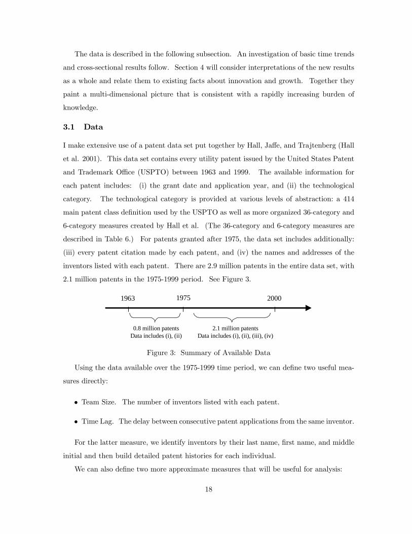
3.1 Data

I make extensive use of a patent data set put together by Hall, Jaffe, and Trajtenberg (Hall

et al. 2001). This data set contains every utility patent issued by the United States Patent

and Trademark Office (USPTO) between 1963 and 1999. The available information for

each patent includes: (i) the grant date and application year, and (ii) the technological

category. The technological category is provided at various levels of abstraction: a 414

main patent class definition used by the USPTO as well as more organized 36-category and

6-category measures created by Hall et al. (The 36-category and 6-category measures are

described in Table 6.) For patents granted after 1975, the data set includes additionally:

(iii) every patent citation made by each patent, and (iv) the names and addresses of the

inventors listed with each patent. There are 2.9 million patents in the entire data set, with

2.1 million patents in the 1975-1999 period. See Figure 3.

1963 1975 2000

0.8 million patentsData includes (i), (ii)

2.1 million patentsData includes (i), (ii), (iii), (iv)

Figure 3: Summary of Available Data

Using the data available over the 1975-1999 time period, we can define two useful mea-

sures directly:

• Team Size. The number of inventors listed with each patent.

• Time Lag. The delay between consecutive patent applications from the same inventor.

For the latter measure, we identify inventors by their last name, first name, and middle

initial and then build detailed patent histories for each individual.

We can also define two more approximate measures that will be useful for analysis:

18

• Tree Size. The size of the citations “tree” behind any patent. Any given patent

will cite a number of other patents, which will in turn cite further patents, and so

on. For the purposes of cross-sectional analysis, the number of nodes in a patent’s

backwards-looking patent tree serves as a proxy measure for the amount of underlying

knowledge.

• Field Jump. The probability that an innovator switches technological areas betweenconsecutive patent applications. This can serve as a proxy measure for the specializa-

tion of innovators. The more specialized you are, the less capable you are of switching

fields.

A limitation of this last measure is that, since technological categories are assigned to

patents and not to innovators, inferring an innovator’s specific field of expertise is difficult

when innovators work in teams. For inventors who work in teams, the relation between

specialization and field jump is in fact ambiguous: as inventors become more specialized and

work in larger teams, they may jump as regularly as they did before. For the specialization

analysis we will therefore focus on solo inventors, for whom increased specialization is always

associated with a decreased capability of switching fields.

Finally, we would like to investigate the age at first innovation. Unfortunately, in-

ventors’ dates of birth are not available in the data set, nor from the USPTO generally.

However, using name and zip code information it was possible to attain birth date infor-

mation for a large subset of inventors through a public website, www.AnyBirthday.com.

AnyBirthday.com uses public records and contains birth date information for 135 million

Americans. The website requires a name and zip code to produce a match. Using a java

program to repeatedly query the website, it was found that, of the 224,152 inventors for

whom the patent data included a zip code, AnyBirthday.com produced a unique match in

56,281 cases. The age data subset and associated selection issues are discussed in detail in

the Data Appendix. The analysis there shows that the age subset is not a random sample

of the overall innovator population. This caveat should be kept in mind when examining

the age results, although it is mitigated by the fact that the differences between the groups

become small when explained by other observables, controlling for these observables in the

age regressions has little effect, and the results for team size, specialization and time lag

persist when looking in the age subset. See the discussion in the Data Appendix.

19

3.2 Time series results

I consider the evolution over time of our four outcomes of interest. Figure 1 presents the

basic data while Tables 2 through 5 examine the time trends in more detail.

Consider team size first. The upper left panel of Figure 1 shows that team size is

increasing at a rapid rate, rising from an average of 1.70 in 1975 to 2.25 at the end of

the period, for a 32% increase overall. Table 2 explores this trend further by performing

regressions relating team size to application year, and we see that the time trend is robust

to a number of controls. Controlling for compositional effects shows that any trends into

certain technological categories or towards patents from abroad have little effect. Repeating

the regressions separately for patents from domestic versus foreign sources shows that the

domestic trend is steeper, though team size is rising substantially regardless of source.

Repeating the time trend regression individually for each of the 36 different technological

categories defined by Hall et al. shows that the upward trend in team size is positive and

highly significant in every single technological category. Running the regressions separately

by “assignee code” to control for the type of institution that owns the patent rights shows

that the upward trend also prevails in each of the seven ownership categories identified

in the data, indicating that the trend is robust across corporate, government, and other

research settings, both in the U.S. and abroad.14 In short, we find an upward trend in

team size that is both general and remarkably steep.

Next consider the age at first innovation. Note that we define an innovator’s “first”

innovation as the first time they appear in the data set. Since we cannot witness individuals’

patents before 1975, this definition is dubious for (i) older individuals, and (ii) observations

of “first” innovations that occur close to 1975. To deal with these two problems, I will

limit the analysis to those people who appear for the first time in the data set between the

ages of 25 and 35 and after 1985. The upper right panel of Figure 1 plots the average age

over time, where we see a strong upward trend. The basic time trend in Table 3 shows an

average increase in age at a rate of 0.66 years per decade. Controlling for compositional

biases due to shifts in technological fields or team size has no effect on the estimates. The

results are also similar when looking at different age windows.15 Analysis of trends within

14Table A.2 describes the ownership assignment categories.15The table reports results for the 23 to 33 age window as well. In results not reported, I find that the

trend is similar across subsets of these windows: ages 23-28, 25-30, 31-35, et cetera. Furthermore, there isno upward trend when looking at age windows beginning at age 35.

20

technological categories shows that the upward trend in age is quite general. Smaller

sample sizes tend to reduce significance when the data is finely cut, but an upward age

trend is found in all 6 technology classes using Hall et al’s 6-category measure, and in 29 of

36 categories when using their 36-category measure. The upward age trend also persists

across all patent ownership classifications.

Now we turn to specialization. The specialization measure considers the probability

that an innovator switches fields between consecutive innovations. Before looking at the

raw data, it is necessary to consider a truncation problem that may bias us toward finding

increased specialization over time. The limited window of our observations (1975-1999)

means that the maximum possible time lag between consecutive patents by an innovator is

largest in 1975 and smallest in 1999. This introduces a downward bias over time in the

lag between innovations. It is intuitive, and it turns out in the data, that people are more

likely to jump fields the longer they go between innovations.16 Mechanically shorter lags

as we move closer to 1999 can therefore produce an apparent increase in specialization. To

combat this problem, I make use of a conservative and transparent strategy. I restrict the

analysis to a subset of the data that contains only consecutive innovations which were made

within the same window of time. In particular, we will look only at consecutive innovations

when the second application comes within 3 years of the first. Furthermore, we will look

only at innovations which were granted within 3 years of the application.17 This strategy

eliminates the bias problem at the cost of limiting our data analysis to the 1975-1993 period

and making our results applicable only to the sub-sample of “faster” innovators.18 The

lower right panel of Figure 1 shows the trend from 1975-1993.

Table 4 considers the trend in specialization with and without this corrective strategy.

The results there, together with the graphical presentation in Figure 1, indicate a smooth

16An interpretation consistent with the spirit of the model is that people need time to reeducate themselveswhen they jump fields, hence a field jump is associated with a larger time lag.17Looking only at patents where the second application came within 3 years limits our analysis to those

cases where the first application was made before 1997. However, a second issue is that patents are grantedwith a delay — 2 years on average — and only patents that have been granted appear in the data. For a firstpatent applied for in 1996, it is therefore much more likely that we will witness a second patent applied forin 1997 than one applied for in 1999 — introducing further downward bias in the data. To deal completelywith the truncation problem, we will therefore further limit ourselves to patents which were granted within3 years of their application, which means that we will only look at the period 1975-1993.18These restrictions maintain a significant percentage of the original sample. For example, of the 111,832

people who applied successfully for patents in 1975, 81,955 of them received a second patent prior to 2000.Of these 81,955 people for whom we can witness a time lag between applications, 79.8% made their nextapplication within three years. Of those, 88.5% were granted both patents within three years of application.

21

decrease in the probability of switching fields. The decline is again quite steep. Using

the central estimate for the trend of -.003, we can interpret a 6% increase in specialization

every ten years. Note that our main results, and Figure 1, use the 414-category measure

for technology to determine whether a field switch has occurred. This is our most accurate

measure of technological field (Hall et al.’s measures are aggregations of it), but the results

are not influenced by the choice of field measure. Note in particular that the percentage

trend is robust to the choice of the 6, 36, or 414 category measure for technology — the

trend is approximately 6% per decade for all three. Including controls for U.S. patents,

the application time lag, ownership status, and the technological class of the initial patent

has little effect. Furthermore, looking for trends within each of Hall et al.’s 36 categories,

we find that the probability of switching fields is declining in 34 of the 36; the decline is

statistically significant in 20. In sum, we see a robust and strongly decreasing tendency for

solo innovators to switch fields.

Finally, I consider the time lag between an innovator’s innovations. The truncation

bias in the time lag described above, which had little effect with specialization, is of course

crucial here, so we employ the same corrective strategy and look only at the 1975-1993

period and the sub-sample of “faster” innovators. The lower left panel of Figure 1 presents

the data graphically and Table 5 considers the trend with and without various controls.

The regressions show a mild upward trend, but this should be viewed skeptically given

the clearly cyclical behavior we see in the graph. Considering the coefficients on various

controls, we see that bigger teams innovate faster and that part of the mild upward trend

is accounted for by a composition effect — innovators switching into fields where the delay

is longer. What is most interesting about the time lag data becomes apparent only when

we look at trends within technological categories. Here we find a richer story: Most fields

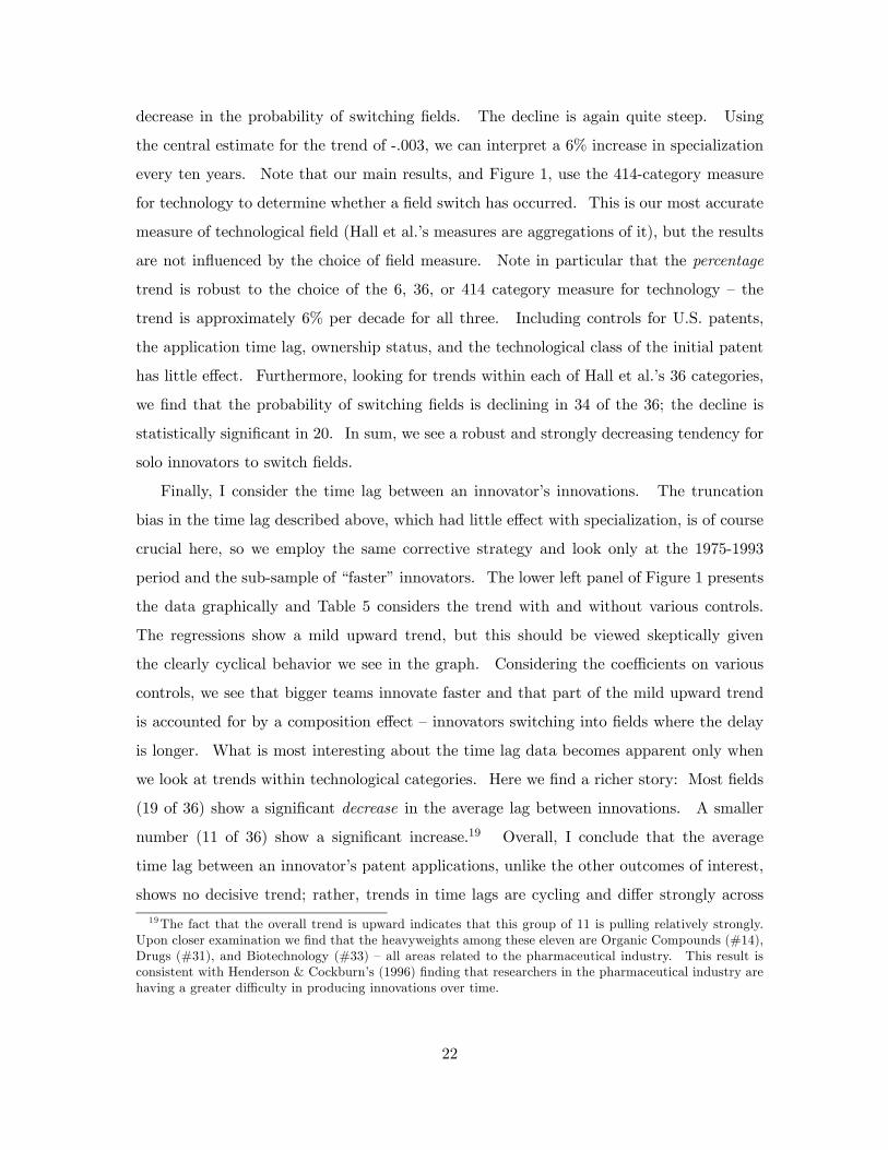
(19 of 36) show a significant decrease in the average lag between innovations. A smaller

number (11 of 36) show a significant increase.19 Overall, I conclude that the average

time lag between an innovator’s patent applications, unlike the other outcomes of interest,

shows no decisive trend; rather, trends in time lags are cycling and differ strongly across

19The fact that the overall trend is upward indicates that this group of 11 is pulling relatively strongly.Upon closer examination we find that the heavyweights among these eleven are Organic Compounds (#14),Drugs (#31), and Biotechnology (#33) — all areas related to the pharmaceutical industry. This result isconsistent with Henderson & Cockburn’s (1996) finding that researchers in the pharmaceutical industry arehaving a greater difficulty in producing innovations over time.

22

technological areas.

3.3 Cross-section results

For a first look at the data in cross-section, Table 6 presents a simple comparison of means

across the 6 and 36 technological categories of Hall et al (2001). The middle column in the

table presents the mean age at first innovation, and the data shows a remarkable consistency

across technological categories. In 30 of the 36 categories, an innovator’s first innovation

tends to come at age 29. The lowest mean age among the 36 categories is 28.8, and the

highest is 31.1, though this last relies on only 12 observations and is an outlier with regard

to the others. The table shows that regardless of whether the invention comes in “Nuclear

& X-rays”, “Furniture, House Fixtures”, “Organic Compounds”, or “Information Storage”,

the mean age at first innovation is nearly the same. According to the cross-sectional

variation of the model, this is what we would expect. Given income arbitrage, innovators

expand their breadth of expertise in shallow areas of knowledge and focus their breadth of

knowledge in deep areas of knowledge so that their educational investment does not differ

across fields.20

The next columns of the table consider the average team size. Here we see large dif-

ferences across technological areas. The largest average team size, 2.90 for the “Drugs”

subcategory, is over twice that of the smallest, 1.41 for the “Amusement Devices” subcate-

gory.

Finally, the last columns of the table consider the probability that a solo innovator will

switch sub-categories between innovations. Here, as with team size and unlike the age at

first innovation, we see large differences across technological areas. This variation is again

consistent with the predictions of the model. At the same time, this basic, cross-sectional

variation in the probability of field jump is difficult to interpret: the probability of field

jump will be tied to how broadly a technological category happens to be defined, which

may vary to a large degree across categories.

I can go further by using a direct measure of the quantity of knowledge underlying a

patent. In particular, I can analyze in cross-section what an increase in the knowledge20These results can also be considered in a regression format. Pooling cross-sections and using application

year dummies to take care of trends, the results are extremely similar. One can also adjust the time at firstinnovation by subtracting category-specific estimates of the time lag to get a closer estimate of an indi-

vidual’s education. One can also look at different age windows. The result that ages are nearly identicalacross fields is highly robust.

23

measure implies for our outcomes of interest.

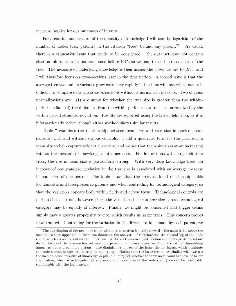
For a continuous measure of the quantity of knowledge I will use the logarithm of the

number of nodes (i.e., patents) in the citation “tree” behind any patent.21 As usual,

there is a truncation issue that needs to be considered: the data set does not contain

citation information for patents issued before 1975, so we tend to see the recent part of the

tree. The measure of underlying knowledge is then noisier the closer we are to 1975, and

I will therefore focus on cross-sections later in the time period. A second issue is that the

average tree size and its variance grow extremely rapidly in the time window, which makes it

difficult to compare data across cross-sections without a normalized measure. Two obvious

normalizations are: (1) a dummy for whether the tree size is greater than the within-

period median; (2) the difference from the within-period mean tree size, normalized by the

within-period standard deviation. Results are reported using the latter definition, as it is

informationally richer, though either method shows similar results.

Table 7 examines the relationship between team size and tree size in pooled cross-

sections, with and without various controls. I add a quadratic term for the variation in

team size to help capture evident curvature, and we see that team size rises at an increasing

rate as the measure of knowledge depth increases. For innovations with larger citation

trees, the rise in team size is particularly strong. With very deep knowledge trees, an

increase of one standard deviation in the tree size is associated with an average increase

in team size of one person. The table shows that the cross-sectional relationship holds

for domestic and foreign-source patents and when controlling for technological category, so

that the variation appears both within fields and across them. Technological controls are

perhaps best left out, however, since the variations in mean tree size across technological

category may be equally of interest. Finally, we might be concerned that bigger teams

simply have a greater propensity to cite, which results in larger trees. This concern proves

unwarranted. Controlling for the variation in the direct citations made by each patent, we

21The distribution of the raw node count within cross-section is highly skewed — the mean is far above themedian, so that upper tail outliers can dominate the analysis. I therefore use the natural log of the nodecount, which serves to contain the upper tail. A (loose) theoretical justification is knowledge depreciation:distant layers of the tree are less relevant to a patent than nearer layers, so there is a natural diminishingimpact as nodes grow more distant. The diminishing impact of the large, distant layers, which dominatethe node counts, is captured loosely by taking logs. Noting that the basic results are similar when we usethe median-based measure of knowledge depth (a dummy for whether the raw node count is above or belowthe median, which is independent of any monotonic transform of the node count) we can be reasonablycomfortable with the log measure.

24

find that relationship actually strengthens. In fact, we see that bigger teams tend to cite

less. This result gives us greater faith in the causative arrow implied by the regressions.

Next we turn to the age at first innovation. Table 8 examines, in pooled cross-sections,

the relationship between age and knowledge for those individuals for whom we can be

confident that they are innovating for the first time (see discussion above). The general

conclusion from the table is that we must work hard to find a relationship, and at its largest

it is very small. It is not robust to the specific age window, is reduced when controlling

for the technological category, and disappears when controlling for the number of direct

citations made. Taking a coefficient of 0.1 as the maximum estimate from the table, we

find that an increase of one standard deviation in the knowledge measure leads to a 0.1

year increase in age. This coefficient may be attenuated given that our proxy measure of

knowledge is, at best, noisy, but I conclude that there is at most only a weak relationship

between the amount of knowledge underlying a patent and the age at first innovation.

Finally, Table 9 considers the relationship between the probability of field jump and the

knowledge measure. The table shows a robust negative relationship: solo innovators are

less likely to jump fields when their initial patent has a larger node count. If we identify a

larger node count with a deeper area of knowledge, then this negative correlation is again

consistent with the predictions of the model. However, I place less emphasis on this result.

The fact that the node count captures the recent part of the tree means that the measure

is likely correlated not just with the total underlying knowledge but also with the recent

ease of innovation. This effect could also explain the negative correlation. Innovators will

be less likely to leave a fruitful area, which will be registered as a decreased probability of

jumping fields.

4 Discussion

This paper is built on two observations. First, innovators are not born at the frontier of

knowledge but must initially undertake significant education. Second, the distance to the

frontier shifts over time. I investigate equilibrium implications of these two observations

and then test these implications empirically. In this section I will review the results and

consider them further in light of existing literatures. Two suggestive conclusions are drawn.

First, human capital decisions appear first-order in understanding important variations in

25

innovative activity across fields and over time. Second, a subset of the evidence points to

a rising burden of knowledge.

The empirical work of Section 3 produces six key facts. We find that the age at first

innovation is increasing over time while it shows no variation across widely different fields, as

demanded by the theory. Meanwhile, team size and specialization are increasing over time

and varying across fields, with greater teamwork and specialization the larger a measure for

the amount of underlying knowledge. These time-series and cross-sectional patterns are

all robust to many controls. The upward trends in age, teamwork, and specialization are

robust across widely different technological areas and research environments. The upward

trends in teamwork and specialization are also especially steep: teamwork is increasing by

17% per decade and the specialization measure by 6% per decade.

Interestingly, some similar trends have been documented elsewhere — and in research

environments outside of patenting. The age at which individuals complete their doctorates

rose generally across all major fields from 1967-1986, with the increase explained by longer

periods in the doctoral program (National Research Council, 1990). The duration of

doctorates as well as the frequency of post-doctorates has been rising across the life-sciences

since the 1960s (Tilghman et al, 1998). An upward age trend has also been noted among

the great inventors of the 20th Century at the age of their noted achievement (Jones, 2005),

as shown in Table 1. Meanwhile, like the general trends in innovator teamwork documented

here, upward trends in academic coauthorship have been documented in many academic

literatures, including physics and biology (Zuckerman & Merton, 1973), chemistry (Cronin

et al, 2004), mathematics (Grossman, 2002), psychology (Cronin et al, 2003), and economics

(McDowell & Melvin, 1983; Hudson, 1996; Laband & Tollison, 2000). These coauthorship

studies show consistent and, collectively, general upward trends, with some of the data sets

going back as far as 1900.

The burden of knowledge mechanism can also speak to trends in the data aggregates

currently debated in the growth literature. First of all, as indicated in Section 2.6, an

increasing burden of knowledge provides one explanation for why high growth rates in the

number of R&Dworkers have not led to increases in rates of TFP growth. Of further interest

is the drop in total patent production per total researchers, which has been documented

across a range of countries and industries and may go back as far as 1900 and even before

(Machlup 1962). Certainly, not all researchers are engaging in patentable activities, and

26

it is possible that much of this trend is explained by relatively rapid growth of research in

basic science.22 However, the results here indicate that among those specific individuals

who produce patentable innovations, the ratio of patents to individuals is in fact declining.

In particular, the recent drop in patents per U.S. R&D worker, a drop of about 50% since

1975 (see Segerstrom 1998), is roughly consistent in magnitude with the rise in team size

over that period. With the time lag between innovations showing little if any deterministic

trend, we have a simple explanation for where these extra innovators have recently been

going — into bigger teams.

In all, the micro-evidence presented in this paper, together with other available micro-

evidence and the aggregate data trends cited above, suggest general and multi-dimensional

patterns that may all be understood within the knowledge burden model. While any indi-

vidual piece of evidence could be explained by other means, the burden of knowledge model

knits together a wide range of evidence within a single framework. Thinking carefully

about the human capital investments faced by innovators leads to precise and empirically

relevant cross-sectional and dynamic insights. Moreover, while the model has relevant or-

ganizational and growth implications regardless of whether the burden of knowledge rises or

falls with time, the evidence suggests specifically that the burden of knowledge is increasing.

The model delivers this inference directly through increasing specialization and teamwork,

but note further that a combination of greater specialization and greater educational attain-

ment is especially difficult to reconcile without appealing to a greater knowledge burden. If

innovators are becoming more specialized but the distance to the frontier is not increasing,

then innovators should have required less education over time.

As emphasized in the model, the knowledge burden channel is not dispositive of other

mechanisms, which operate independently and may also be important to innovator out-

put. The general equilibrium setting of the model explicitly embraces popular stories in

the literature regarding innovation exhaustion ("fishing out" stories), increasing innovation

potential, and market size effects. Fishing-out stories are particularly interesting because

they can provide an alternative or additional explanation for the data aggregates — patterns

which have motivated that literature. While the trends in the data regarding team size, age,

or specialization appear orthogonal to a fishing-out story, this orthogonality leaves room

22Such an explanation could be inferred from the observations of Mokyr (1990), for example, who sees anincreasing role for basic science as a foundation for technological advance.

27

for a fishing-out mechanism alongside a rising burden of knowledge when one confronts

aggregate data.23 Defining precise micro-data tests for a fishing-out story is a challenge

for future research. Differentiating between a fishing-out and knowledge burden mecha-

nism is challenging on the basis of productivity alone, as any decrease in the size or rate of

innovations can be explained by either narrowing expertise or innovation exhaustion.

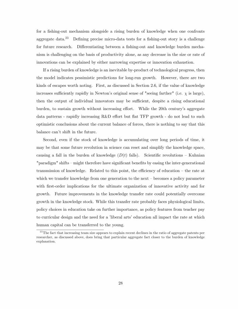
If a rising burden of knowledge is an inevitable by-product of technological progress, then

the model indicates pessimistic predictions for long-run growth. However, there are two

kinds of escapes worth noting. First, as discussed in Section 2.6, if the value of knowledge

increases sufficiently rapidly in Newton’s original sense of "seeing farther" (i.e. χ is large),

then the output of individual innovators may be sufficient, despite a rising educational

burden, to sustain growth without increasing effort. While the 20th century’s aggregate

data patterns - rapidly increasing R&D effort but flat TFP growth - do not lead to such

optimistic conclusions about the current balance of forces, there is nothing to say that this

balance can’t shift in the future.

Second, even if the stock of knowledge is accumulating over long periods of time, it

may be that some future revolution in science can reset and simplify the knowledge space,

causing a fall in the burden of knowledge (D(t) falls). Scientific revolutions — Kuhnian

"paradigm" shifts — might therefore have significant benefits by easing the inter-generational

transmission of knowledge. Related to this point, the efficiency of education — the rate at

which we transfer knowledge from one generation to the next — becomes a policy parameter

with first-order implications for the ultimate organization of innovative activity and for

growth. Future improvements in the knowledge transfer rate could potentially overcome

growth in the knowledge stock. While this transfer rate probably faces physiological limits,

policy choices in education take on further importance, as policy features from teacher pay

to curricular design and the need for a ’liberal arts’ education all impact the rate at which

human capital can be transferred to the young.

23The fact that increasing team size appears to explain recent declines in the ratio of aggregate patents perresearcher, as discussed above, does bring that particular aggregate fact closer to the burden of knowledgeexplanation.

28

5 Appendix

Proof of Proposition 1.iL(t, s) = LR(t) ∀s

First I generalize the innovator’s income function to allow the possibility that not allideas are feasible to implement. Then I show that innovators will array themselves evenlyaround the circle.

(1) Define pi(t) such that ∀k > pi(t) the necessary teammates do not exist and ∀k ≤ pi(t)

the necessary teammates do exist. The probability that an idea k is feasible is then F (pi(t)).The innovator’s expected income at the time of their birth t0 is a generalized version of (5)that allows for the possibility that an idea is infeasible:

b∗βi

Z ∞

t0F (pi(t))X(t)

χL(t, s0)−σM(t)e−φ(t−t0)dt− ¡b∗iD(t0)¢ε (20)

Note that, in any equilibrium, b∗i > 0 and F (pi(t)) > 0 by the arbitrage condition (12),since otherwise UR&D

i = 0 but Uwage > 0. Moreover, there must exist an arbitrarily smallsuch that 0 < < b∗i .(2) By contradiction, imagine that

L(t, s0) > L(t, s00)

where s0 > s00 > s0 − . That is, there exist two neighboring points, a relatively crowdedpoint s0 and a less crowded point s00. Without loss of generality, choose individual i at s0

such that b∗i ≤ bj for some j at s0, j 6= i. If this individual i at s0 were to shift to s00,then the access to potential teammates remains unchanged. (The individual can alwayshire someone in L(t0, s0) as a teammate, and everyone else at that point has weakly greaterexpertise.) Therefore bpi(t) = pi(t)+ , and the probability that an idea k is feasible is weaklyincreasing with this deviation since for any distribution function F (pi(t) + ) ≥ F (pi(t).

Therefore, from (20) and the equilibrium condition (11), the choice s0 (i.e. the crowdedlocation) can only be an equilibrium for person i ifZ ∞

t0L(t, s0)−σX(t)χM(t)e−φ(t−t

0)dt ≥Z ∞

t0L(t, s00)−σX(t)χM(t)e−φ(t−t

0)dt (21)

Given the continuity of L with time, L(t, s0) > L(t, s00) for all t in some interval [t0, t00].Therefore, the expected income to innovator i in the interval [t0, t00] must be strictly lesswith the crowded choice s0 then with the less crowded choice s00. Therefore, innovator imust believe thatZ ∞

t00L(t, s0)−σX(t)χM(t)e−φ(t−t

0)dt >

Z ∞

t00L(t, s00)−σX(t)χM(t)e−φ(t−t

0)dt (22)

That is, eventually the relatively crowded choice must produce greater income. But multi-plying both sides of this expression by the constant e−φ(t0−t00), we see that in the subgamefor those born at time t00 no person would choose s00. Hence L (t00, s00) is not increasing,L(t00, s0) > L(t00, s00), and there is no finite t00 at which (22) holds. Hence (21) cannot hold.Hence, by contradiction, no such point s00 can exist and therefore there can be no points onthe circle where the mass is less than any other point. QED.

29

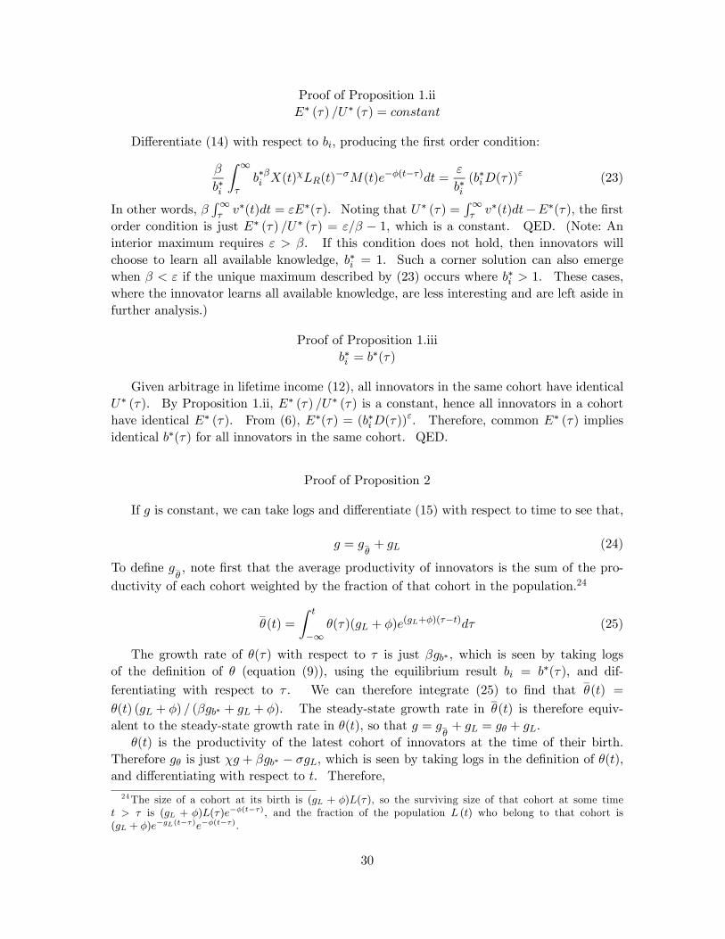
Proof of Proposition 1.iiE∗ (τ) /U∗ (τ) = constant

Differentiate (14) with respect to bi, producing the first order condition:

β

b∗i

Z ∞

τb∗βi X(t)χLR(t)

−σM(t)e−φ(t−τ)dt =ε

b∗i(b∗iD(τ))

ε (23)

In other words, βR∞τ v∗(t)dt = εE∗(τ). Noting that U∗ (τ) =

R∞τ v∗(t)dt−E∗(τ), the first

order condition is just E∗ (τ) /U∗ (τ) = ε/β − 1, which is a constant. QED. (Note: Aninterior maximum requires ε > β. If this condition does not hold, then innovators willchoose to learn all available knowledge, b∗i = 1. Such a corner solution can also emergewhen β < ε if the unique maximum described by (23) occurs where b∗i > 1. These cases,where the innovator learns all available knowledge, are less interesting and are left aside infurther analysis.)

Proof of Proposition 1.iiib∗i = b∗(τ)

Given arbitrage in lifetime income (12), all innovators in the same cohort have identicalU∗ (τ). By Proposition 1.ii, E∗ (τ) /U∗ (τ) is a constant, hence all innovators in a cohorthave identical E∗ (τ). From (6), E∗(τ) = (b∗iD(τ))

ε. Therefore, common E∗ (τ) impliesidentical b∗(τ) for all innovators in the same cohort. QED.

Proof of Proposition 2

If g is constant, we can take logs and differentiate (15) with respect to time to see that,

g = g_θ+ gL (24)

To define g_θ, note first that the average productivity of innovators is the sum of the pro-

ductivity of each cohort weighted by the fraction of that cohort in the population.24

_θ(t) =

Z t

−∞θ(τ)(gL + φ)e(gL+φ)(τ−t)dτ (25)

The growth rate of θ(τ) with respect to τ is just βgb∗ , which is seen by taking logsof the definition of θ (equation (9)), using the equilibrium result bi = b∗(τ), and dif-ferentiating with respect to τ . We can therefore integrate (25) to find that

_θ(t) =

θ(t) (gL + φ) / (βgb∗ + gL + φ). The steady-state growth rate in_θ(t) is therefore equiv-

alent to the steady-state growth rate in θ(t), so that g = g_θ+ gL = gθ + gL.

θ(t) is the productivity of the latest cohort of innovators at the time of their birth.Therefore gθ is just χg + βgb∗ − σgL, which is seen by taking logs in the definition of θ(t),and differentiating with respect to t. Therefore,24The size of a cohort at its birth is (gL + φ)L(τ), so the surviving size of that cohort at some time

t > τ is (gL + φ)L(τ)e−φ(t−τ), and the fraction of the population L (t) who belong to that cohort is(gL + φ)e−gL(t−τ)e−φ(t−τ).

30

g_θ= χg + βgb∗ − σgL (26)

Note that E∗/U∗ is constant (Proposition 1.ii), which implies gE∗ = gU∗ . Furthermore,from (13), gU∗ = g, which implies gE∗ = g. From (6), gE∗ = 1/ε (gb∗ − gD), and from (7),gD = δg. Therefore gb∗ = (1ε − δ)g, a result presented in (17).

Inserting (17) into (26), the result into (24), and rearranging produces the expressionfor steady-state growth in equation (16). QED.

Proof of Corollary 1.igE∗ = g

E∗/U∗ is constant (Proposition 1.ii), which implies gE∗ = gU∗ . From (13), gU∗ = g.Therefore, gE∗ = g. QED

Proof of Corollary 1.iigb∗ < 0 iff δ > 1/ε

The growth rate of b∗ is given in (??). Hence gb∗ < 0 iff δ > 1/ε. QED.

Proof of Corollary 1.iiiteam(t) > 0 iff δ > 1/ε

Recall that k, the breadth of expertise required to implement an idea, has a smoothdistribution function F (k). A cohort with breadth of expertise b will therefore produce ateam of size 1 with probability F (b), a team of size 2 with probability F (2b) − F (b), andso on. Recall also that teams are formed within cohorts if possible and with the minimumpossible number of individuals (see Section 2.4). Since individuals allocate themselvesevenly around the circle in any cohort (Proposition 1.i), any necessary teammates are alwaysavailable within one’s own cohort. This implies that teams are formed from individualswith identical choices of b, b∗(τ) (Proposition 1.iii). Since teams are formed from theminimum number of individuals, the implementation of any idea k requires d(k/b) teammembers; that is, k/b rounded up to the nearest integer. The maximum team size in acohort with breadth of expertise b is defined by n = d(1/b). The expected team size isteam(b) = 1F (b) + 2(F (2b) − F (b)) + ... + n(1 − F ((n − 1)b). Collecting terms in thisexpression, team(b) = n −Pn−1

j=1 F (jb) where j indexes a particular realization of team

size. Differentiating with respect to b shows that, dteam(b)/db = −Pn−1j=1 jf(jb) where

f(k) = dF/dk is the probability density function corresponding to F . Given that a densityfunction is weakly positive at any point, we see that team size is weakly increasing as bfalls. Hence the conditions for average team size to increase with time are identical to thecondition for expertise to narrow; i.e. if and only if δ > 1/ε. QED.

31

Extension to Corollary 1.iiiA generalized condition for team size to increase with specialization

I explore here the evolution of team size when the distribution of k changes with anindividual’s breadth of expertise, b. Define the generalized distribution function by F (k; b)and the corresponding density function as f(k; b) = dF (k; b)/dk. The average team size fora cohort with breadth of expertise b is derived just as in (??),

team(b) = n−n−1Xj=1

F (jb; b) (27)

Noting that F (jb; b) =R jb0 f(k; b)dk, we can use Leibniz’s rule to differentiate (27) with

respect to b and thereby define a necessary and sufficient condition for team size to increasewith specialization:

n−1Xj=1

µZ jb

0

df(k; b)

dbdk + jf(jb; b)

¶> 0⇔ dteam(b)

db< 0 (28)

The second term on the left hand side is recognized from equation (??) and acts to maketeam size increase with specialization. The effect of the first term is ambiguous, how-ever, so that the effect of specialization on team size cannot be signed without consideringdistribution-specific properties.

We can gain some intuition for this condition by considering the simple case where kis drawn from a uniform distribution. Specifically, let k ∼ U [0, bα], so that f(k; b) = b−α.Using (28), it is then straightforward to show that α < 1⇔ dteam(b)/db < 0. Noting thatthe mean of k is E (k) = 1

2bα, it is also straightforward to show that α is the elasticity of E(k)

with respect to b. Therefore, we see that team size will be increasing with specializationso long as the elasticity of E(k) with respect to expertise is less than 1. In other words,team size will be increasing as long as innovators’ average “reach”, given by E(k), does notdecline faster than their average “grasp”, given by b.

Proof of Proposition 3

The proof follows exactly the same structure as the proof of Proposition 1 and is omittedfor brevity.

Proof of Corollary 2.iE∗ij(τ) = E∗(τ) ∀i, j

Arbitrage implies a common U∗ (τ) within every cohort. Since E∗(τ)/U∗ (τ) is a con-stant (Proposition 3.ii), every innovator must choose the same E∗(τ). QED.

Proof of Corollary 2.iib∗j(τ) < b∗j0(τ) iff Dj(τ) > Dj0(τ)

32

All innovators in a cohort, by Corollary 2.i, choose the same amount of education,

E∗(τ) =³b∗j (τ)Dj (τ)

´ε. Therefore b∗j (τ)Dj (τ) = b∗j0 (τ)Dj0 (τ) ∀j, j0 and hence the

corollary 2.ii. QED.

Proof of Corollary 2.iiiteamj (τ) > teamj0 (τ) iff Dj(τ) > Dj0(τ)

By Corollary 2.ii, an innovator cohort within a circle of knowledge j will have narrowerexpertise the greater the depth of knowledge. By the same logic as in the proof of Corollary1.iii, narrower expertise is associated with larger team size. QED

Extended Model: A Time Cost to Education

The following model is a generalization of the model in the text. The model in the textallows for an additively separable cost of education, E, where this cost can be thought ofas either an out-of-pocket expense or a direct utility cost of effort. Here I will introduce anadditional opportunity cost of education: choosing more education results in a longer periodat the beginning of life when one does not earn income. In particular, define T = α ln(bD)

as the duration of education., which is monotonically increasing in the amount of knowledgelearned, bD. The model is as before, except innovator income is defined by

UR&Di (τ) =

Z ∞

τ+Tvi(t)e

−φ(t−τ)dt−Ei(τ) (29)

in place of (5).Equilibrium analysis follows mostly as before. The equilibrium choice of s still requires

that innovators spread out evenly around the circle. The equilibrium choice of b∗i becomesanalytically more tedious, as the choice of breadth of expertise now additionally affects onelimit of the integral in (29). Using Leibniz’s rule in differentiating (29), in addition to thedefinitions of v and E in (10) and (6), we can write the first-order condition for the choiceof b, with some manipulation, as:

β − εE∗(τ)Π∗ (τ)

= b∗i∂T

∂b∗i

v∗i (τ + T ) e−φT ∗

Π∗ (τ)(30)

where Π (τ) ≡ R∞τ+T vi(t)e

−φ(t−τ)dt. This is a generalization of (23) — the simpler casewith no time-cost, where the right hand side of (30) is zero (∂T/∂b = 0). Here, given thedefinition of T , b∗i ∂T/∂b∗i = α. To analyze v∗i (τ + T ) e−φT ∗/Π∗ (τ), we will proceed byfocusing on the equilibrium along a balanced-growth path. On the balanced growth path,X grows at rate g, while LR and M grow at rate gL. Under these conditions, it is easilyshown that v∗i (τ + T ) e−φT ∗/Π∗ (τ) = φ + χg + (σ − 1) gL. Therefore, E∗(τ)/Π∗ (τ) =β/ε− (α/ε) (φ+ χg + (σ − 1) gL). Noting that U∗ (τ) = Π∗ (τ)−E∗(τ), we have the result

E∗(τ)/U∗ (τ) = constant

33

In other words, we have the same result as Proposition 1.ii (with the exception that we arenow focusing on the steady-state growth path), from which Proposition 1.iii, Proposition3, and Corollaries 1 and 2 will follow. Since both E and T are monotonically increasingin the amount of knowledge learned (bD), rising E∗ along the growth path (Corollary 1.i)implies that T ∗, the duration of education, also rises along the growth path. Similarly,common E∗ across fields (Corollary 2.i) implies that T ∗ is the same across fields.

The one set of results that must be generalized is Proposition 2, which defines thesteady-state growth rate. The steady-state growth rate is now an implicit function of themodel parameters. (The derivation follows along the lines of the proof of Proposition 2).In the special case that α = 0, so that there is no time-cost to education, the steady-stategrowth is given by (16), as before. In the special case where specialization doesn’t changewith time (ε = 1/δ), the growth rate is given by

g =1− σ

1− χ+ α/ε(φ+ gL)gL

Here the effect of the burden of knowledge on growth is felt entirely through the timecost of education. Larger values of the parameter α, which implies a higher sensitivityof educational duration to the amount of knowledge one learns, causes lower growth rates,since one spends a smaller portion of the one’s life-cycle actively producing innovations.

6 Data Appendix

The reader is referred to Hall et al (2001) for a detailed discussion of their patent data set.This appendix focuses on the age information collected to augment the Hall et al data.

Age data was collected using the website www.AnyBirthday.com, which requires a nameand zip code to produce a match. As is seen in Table A.1, 30% of U.S. inventors listed a zipcode on at least one of their patent applications, and of these inventors AnyBirthday.comproduced a birth date in 25% of the cases. While the number of observations producedby AnyBirthday.com is large, it represents only 7.5% of U.S. inventors. This Appendixexplores the causes and implications of this selection. The first question is why zip codeinformation is available for only certain inventors. The second question is why AnyBirth-day.com produces a match only one-quarter of the time. The third question is whetherthis selection appears to matter.

Table A.2 compares how patent rights are assigned across samples. The table showsclearly that zip code information is virtually always supplied when the inventor has yetto assign the rights; conversely, zip code information is never provided when the rightsare already assigned. Patent rights are usually assigned to private corporations (80% ofthe time) and remain unassigned in the majority of the other cases (17% of the time).An unassigned patent indicates only that the inventor(s) have not yet assigned the patentat the time it is granted. Presumably, innovators who provide zip codes are operatingoutside of binding contracts with corporations, universities, or other agencies that wouldautomatically acquire any patent rights. The zip-code subset is therefore not a randomsample, but is capturing a distinct subset of innovators who, at least at one point, wereoperating independently. Despite this distinction, this subset may not be substantially

34

different from other innovators: the last column of Table A.2 indicates that, when lookingat the other patents produced by these innovators, they have a similar propensity to assignthem to corporations as the U.S. population average.

The nature of the selection introduced by AnyBirthday.com is more difficult to iden-tify. The website reports a database of 135 million individuals and reports to have builtits database using “public records”. Access to public records is a contentious legal issue.25

Public disclosure of personal information is proscribed at the federal level by the Freedomof Information Act and Privacy Act of 1974. At the state and local level however, rulesvary. Birth date and address information are both available through motor vehicle depart-ments and their electronic databases are likely to be the main source of AnyBirthday.com’srecords.26 The availability of birth date information is therefore very likely to be relatedto local institutional rules regarding motor vehicle departments. Geography thus will in-fluence the presence of innovators in the age sample, and a further issue in selection mayinvolve the geographic mobility of the innovator, among other factors. The influence of thisselection, together with the implications of assignment status, can be assessed by comparingobservable means in the population across subsamples.

Table A.3 considers average team size, which is a source of further differences. Patentswith provided zip codes have smaller team sizes than the U.S. average; team sizes in thesubset of these patents for which the age of one innovator is known are slightly larger, butstill smaller than the U.S. average. Controlling for other patent observables, in particularthe assignment status, reduces the mean differences and brings the age sample quite closelyin line with the U.S. mean. (See the last two columns of the table.) Having examined anumber of other observables in the data, such as citations received and average tree size,I find that relatively small differences tend to exist in the raw data, and that these canbe either entirely or largely explained by controlling for assignment status and team size.Most importantly, the age results in the text are all robust to the inclusion of assignmentstatus, team size, and any other available controls.

Finally, looking at team size, specialization, and time lag trends in the age subsample,the results are similar in sign and significance as those presented in Section 4. The rate ofincrease in specialization is larger, and the rate of increase in team size is smaller. The timelag shows no trend. Reexamining trends in the entire data set by assignment status, I findthat the team size trend is weaker among the unassigned category, which likely explains theweaker trend in the age subset. Similarly, I find that the specialization trend is strongeramong the unassigned category, which likely explains the stronger trend in the age subset.

I conclude therefore that while the age subset is not a random sample of the U.S.innovator population, the differences tend to be explainable with other observables and, onthe basis of including such observables in the analysis, the age results appear robust.

25Repeated requests to AnyBirthday.com to define their sources more explicitly have yet to produce aresponse.26A federal law, the Driver’s Privacy Protection Act of 1994, was introduced to give individuals increased

privacy. The law requires motor vehicle departments to receive explicit prior consent from an individualbefore disclosing their personal information. However, the law makes an exception for cases where motorvehicles departments provide information to survey and marketing organizations. In that case, individual’sconsent is assumed unless the individual has opted-out on their own initiative. See Gellman (1995) for anin-depth discussion of the laws and legal history surrounding public records.

35

References

[1] Aghion, Philippe and Howitt, Peter. “A Model of Growth through Creative Destruc-tion,” Econometrica, March 1992, 60, 323-351.

[2] ––. Endogenous Growth Theory, Cambridge, MA: MIT Press, 1998.

[3] Baily, Martin N. and Chakrabarti, Alok K. “Innovation and Productivity in U.S.Industry,” Brookings Papers on Economic Activity, 1985, 609-632.

[4] Ben-Porath, Yoram. “The Production of Human Capital and the Life Cycle of Earn-ings,” Journal of Political Economy, August 1967, 75, 352-365.

[5] Cronin, Blaise, Shaw, Debora, and La Barre, Kathryn. "A Cast of Thousands: Coau-thorship and Subauthorship Collaboration in the 20th Century as Manifested in theScholarly Journal Literature of Psychology and Philosophy," Journal of the AmericanSociety for Information Science and Technology, 2003, 54(9), 855-871.

[6] ––. "Visible, Less Visible, and Invisible Work: Patterns of Collaboration in 20thCentury Chemistry," Journal of the American Society for Information Science andTechnology, 2004, 55(2), 160-168.

[7] Evenson, Robert E. “International Invention: Implications for Technology MarketAnalysis,” in Zvi Griliches, ed., R&D, Patents, and Productivity, Chicago, IL: Univer-sity of Chicago Press, 1984, 89-123.

[8] ––. "Patent Data by Industry: Evidence for Invention Potential Exhaustion?"Technology and Productivity: The Challenge for Economic Policy, 1991, Paris: OECD,233-248.

[9] Gellman, Robert. “Public Records: Access, Privacy, and Public Pol-icy,” Center for Democracy and Technology Discussion Paper, April 1995,http://www.cdt.org/privacy/pubrecs/pubrec.html.

[10] Grossman, Gene M. and Helpman, Elhanan. Innovation and Growth in the GlobalEconomy, Cambridge, MA: MIT Press, 1991.

[11] Grossman, Jerry. "The Evolution of the Mathematical Research Collaboration Graph,"Congressus Numerantium, 2002, 158, 202-212.

[12] Hall, Bronwyn H., Jaffe, Adam B., and Trajtenberg, Manuel. “The NBER PatentCitations Data File: Lessons, Insights and Methodological Tools,” NBER WorkingPaper No. 8498, October 2001.

[13] Hart, Oliver and Moore, John. “A Theory of Debt Based on the Inalienability ofHuman Capital,” Quarterly Journal of Economics, November 1994, 109, 841-879.

[14] Henderson, Rebecca and Cockburn, Iain. “Scale, Scope, and Spillovers: The Deter-minants of Research Productivity in Drug Discovery,” Rand Journal of Economics,Spring 1996, 27, 32-59.

[15] Hudson, John. "Trends in Multi-Authored Papers in Economics," Journal of EconomicPerspectives, Summer 1996, 10, 153-158.

[16] Jones, Benjamin F. “Age and Great Invention,” NBERWorking Paper #(TBD), 2005.

[17] Jones, Charles I. “R&D-Based Models of Economic Growth,” Journal of PoliticalEconomy, August 1995, 103, 759-784.

36

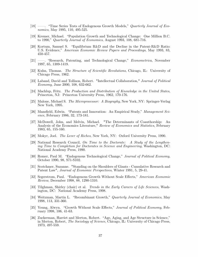
[18] ––. “Time Series Tests of Endogenous Growth Models,” Quarterly Journal of Eco-nomics, May 1995, 110, 495-525.

[19] Kremer, Michael. “Population Growth and Technological Change: One Million B.C.to 1990,” Quarterly Journal of Economics, August 1993, 108, 681-716.

[20] Kortum, Samuel S. “Equilibrium R&D and the Decline in the Patent-R&D Ratio:U.S. Evidence,” American Economic Review Papers and Proceedings, May 1993, 83,450-457.

[21] ––. “Research, Patenting, and Technological Change,” Econometrica, November1997, 65, 1389-1419.

[22] Kuhn, Thomas. The Structure of Scientific Revolutions, Chicago, IL: University ofChicago Press, 1962.

[23] Laband, David and Tollison, Robert. "Intellectual Collaboration," Journal of PoliticalEconomy, June 2000, 108, 632-662.

[24] Machlup, Fritz. The Production and Distribution of Knowledge in the United States,Princeton, NJ: Princeton University Press, 1962, 170-176.

[25] Malone, Michael S. The Microprocessor: A Biography, New York, NY: Springer-VerlagNew York, 1995.

[26] Mansfield, Edwin. “Patents and Innovation: An Empirical Study,” Management Sci-ence, February 1986, 32, 173-181.

[27] McDowell, John, and Melvin, Michael. "The Determinants of Coauthorship: AnAnalysis of the Economics Literature," Review of Economics and Statistics, February1983, 65, 155-160.

[28] Mokyr, Joel. The Lever of Riches, New York, NY: Oxford University Press, 1990.

[29] National Research Council, On Time to the Doctorate: A Study of the Lengthen-ing Time to Completion for Doctorates in Science and Engineering, Washington, DC:National Academy Press, 1990.

[30] Romer, Paul M. “Endogenous Technological Change,” Journal of Political Economy,October 1990, 98, S71-S102.

[31] Scotchmer, Suzanne. "Standing on the Shoulders of Giants - Cumulative Research andPatent Law", Journal of Economic Perspectives, Winter 1991, 5, 29-41.

[32] Segerstrom, Paul. “Endogenous Growth Without Scale Effects,” American EconomicReview, December 1998, 88, 1290-1310.

[33] Tilghman, Shirley (chair) et al. Trends in the Early Careers of Life Sciences, Wash-ington, DC: National Academy Press, 1998.

[34] Weitzman, Martin L. “Recombinant Growth,” Quarterly Journal of Economics, May1998, 113, 331-360.

[35] Young, Alwyn. “Growth Without Scale Effects,” Journal of Political Economy, Feb-ruary 1998, 106, 41-63.

[36] Zuckerman, Harriet and Merton, Robert. “Age, Aging, and Age Structure in Science,”in Merton, Robert, The Sociology of Science, Chicago, IL: University of Chicago Press,1973, 497-559.

37

38

Table 1: Age Trends among Great Innovators

Dependent Variable: Age at Great Achievement Nobel Prize Winners Great Inventors

Year of Great Achievement

(in 100’s)

5.83*** (1.37)

4.86** (2.31)

Number of observations

544

286

Time span

1873-1998

1900-91

Average age

38.6

39.0

R2

0.032

0.016

NOTES: (i) This table borrows from Jones (2005). Age trends are measured in years per century. Standard errors are given in parentheses. (ii) Nobel Prize winners include all winners in Physics, Chemistry, Medicine, and Economics. Great inventors are taken from technological almanacs listing the great inventions of the 20th century. **Indicates 95% confidence level. ***Indicates 99% confidence level.

39

Table 2: Trends in Inventors per Patent

Dependent Variable: Inventors per Patent (1) (2) (3) (4) (5) (6) (7)

Application Year

.0293

(.0001)

.0261

(.0001)

.0262

(.0001)

.0251

(.0001)

.0244

(.0002)

.0306

(.0002)

.0180

(.0003)

Foreign Patent

--

.444

(.002)

.416

(.002)

.141

(.004)

.146

(.004)

US Only

Foreign

Only Broad

--

Yes

--

--

--

--

--

Tech

nolo

gica

l Fi

eld

Con

trols

Narrow

--

--

Yes

Yes

Yes

Yes

Yes

Assignee Code

--

--

--

Yes

Yes

Yes

Yes

Number of Observations

2,016,377

2,016,377

2,016,377

2,016,377

1,506,956

1,123,310

893,067

Period

1975-1999

1975-1999

1975-1999

1975- 1999

1975- 1996

1975-1999

1975-1999

Mean of Dependent Variable

2.03

2.03

2.03

2.03

1.97

1.82

2.29

Per-decade Trend as % of Period Mean

14.4%

12.9%

12.9%

12.4%

12.4%

16.8%

7.9%

R2

.02

.08

.10

.12

.13

.12

.10

NOTES (i) Regressions are OLS with standard errors in parentheses. Specifications (1) through (4) consider the entire universe of patents applied for between 1975 and 1999. Specification (5) considers only patents that were granted within three years after application (see discussion in text). Specifications (6) and (7) present separate trends for domestic and foreign source patents. (ii) Foreign Patent is a dummy variable to indicate whether the first inventor listed with the patent has an address outside the U.S.. (iii) “Broad” technological controls include dummies for each of the 6 categories in Hall et al.’s most aggregated technological classification. “Narrow” technological controls include dummies for each category of their 36-category classification. (iv) Upward trends persist when run separately for each technological field. Using the broad classification (six categories), the trends range from a low of .018 for “Other” to a high of .037 for “Chemical”. Using the narrower classification scheme (thirty-six categories), the trends range from a low of .007 for “Apparel &Textile” to .051 for “Organic Compounds”. The smallest t-statistic for any of these trends is 7.76. (v) Assignee code controls are seven dummy variables that define who holds the rights to the patent. Most patent rights are held by US or foreign corporations (80%), while a minority remain unassigned (17%) at the time the patent is issued. Table A.2 describes the assignee codes in further detail. Running the time trends separately for the individual assignee codes shows that the team size trends range from a low of .005 for the unassigned category to a high of .039 for US non-government institutions. The lowest t-statistic for any of these trends is 5.38.

40

Table 3: Trends in Age at First Innovation

Dependent Variable: Age at Application (1) (2) (3) (4) (5) (6) (7)

Application Year

.0657

(.0095)

.0666

(.0095)

.0671

(.0095)

.0671

(.0099)

.0687

(.0097)

.0530

(.0107)

.0584

(.0109) Broad

--

Yes

--

--

--

--

--

Tech

nolo

gica

l Fi

eld

Con

trols

Narrow

--

--

Yes

Yes

Yes

--

Yes

Assignee Code

--

--

--

Yes

Yes

--

Yes

Team Size

--

--

--

--

-.0630 (.0273)

--

-.0348 (.0306)

Number of observations

6,541

6,541

6,541

6,541

6,541

5,102

5,102

Period

1985-1999

1985-1999

1985-1999

1985-1999

1985-1999

1985-1999

1985-1999

Age Range

25-35 25-35 25-35 25-35 25-35 23-33 23-33

Mean of Dependent Variable

31.0

31.0

31.0

31.0

31.0

29.3

29.3

Per-decade Trend as % of Period Mean

2.1%

2.1%

2.2%

2.2%

2.2%

1.8%

2.0%

R2

.007

.010

.020

.020

.021

.005

.018

NOTES (i) Regressions are OLS, with standard errors in parentheses. All regressions look only at those innovators for whom we have age data and who appear for the first time in the data set in or after 1985. Specifications (1) through (5) consider those innovators who appear for the first time between ages 25 and 35. Specifications (6) and (7) consider those innovators who appear for the first time between ages 23 and 33. (ii) “Broad” technological controls include dummies for each of the 6 categories in Hall et al.’s most aggregated technological classification. “Narrow” technological controls include dummies for each classification in their 36-category measure. The upward age trend persists when run separately in each of Hall et al’s broad technology classes. These trends are significant in 5 of the 6 categories, with similar trend coefficients as when the data are pooled. Upward trends are also found in 29 of 36 categories when using Hall et al.’s narrow technology classification. Here 12 categories show significant upward trends. Sample sizes drop considerably when the data is divided into these 36 categories. The one case of a significant downward trend (category #23, Computer Peripherals) has 42 observations. (iii) Assignee code controls are seven dummy variables that define who holds the rights to the patent. Table A.2 describes the assignee codes in further detail. The upward age trends persist when run separately for each assignee code and are similar in magnitude to the trends in the table above.

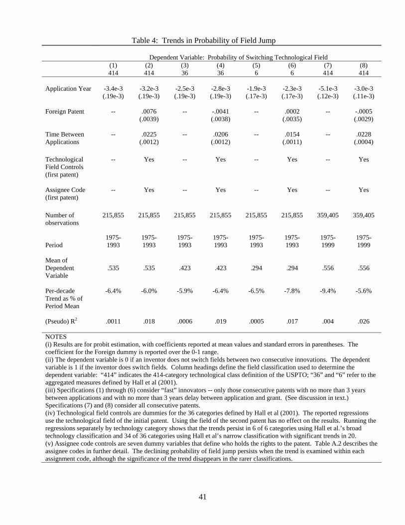
41

Table 4: Trends in Probability of Field Jump

Dependent Variable: Probability of Switching Technological Field (1)

414 (2) 414

(3) 36

(4) 36

(5) 6

(6) 6

(7) 414

(8) 414

Application Year

-3.4e-3 (.19e-3)

-3.2e-3 (.19e-3)

-2.5e-3 (.19e-3)

-2.8e-3 (.19e-3)

-1.9e-3 (.17e-3)

-2.3e-3 (.17e-3)

-5.1e-3 (.12e-3)

-3.0e-3 (.11e-3)

Foreign Patent

--

.0076

(.0039)

--

-.0041 (.0038)

--

.0002

(.0035)

--

-.0005 (.0029)

Time Between Applications

--

.0225

(.0012)

--

.0206

(.0012)

--

.0154

(.0011)

--

.0228

(.0004) Technological Field Controls (first patent)

--

Yes

--

Yes

--

Yes

--

Yes

Assignee Code (first patent)

--

Yes

--

Yes

--

Yes

--

Yes

Number of observations

215,855

215,855

215,855

215,855

215,855

215,855

359,405

359,405

Period

1975-1993

1975-1993

1975-1993

1975-1993

1975-1993

1975-1993

1975-1999

1975-1999

Mean of Dependent Variable

.535

.535

.423

.423

.294

.294

.556

.556

Per-decade Trend as % of Period Mean

-6.4%

-6.0%

-5.9%

-6.4%

-6.5%

-7.8%

-9.4%

-5.6%

(Pseudo) R2

.0011

.018

.0006

.019

.0005

.017

.004

.026

NOTES (i) Results are for probit estimation, with coefficients reported at mean values and standard errors in parentheses. The coefficient for the Foreign dummy is reported over the 0-1 range. (ii) The dependent variable is 0 if an inventor does not switch fields between two consecutive innovations. The dependent variable is 1 if the inventor does switch fields. Column headings define the field classification used to determine the dependent variable: “414” indicates the 414-category technological class definition of the USPTO; “36” and “6” refer to the aggregated measures defined by Hall et al (2001). (iii) Specifications (1) through (6) consider “fast” innovators -- only those consecutive patents with no more than 3 years between applications and with no more than 3 years delay between application and grant. (See discussion in text.) Specifications (7) and (8) consider all consecutive patents. (iv) Technological field controls are dummies for the 36 categories defined by Hall et al (2001). The reported regressions use the technological field of the initial patent. Using the field of the second patent has no effect on the results. Running the regressions separately by technology category shows that the trends persist in 6 of 6 categories using Hall et al.’s broad technology classification and 34 of 36 categories using Hall et al’s narrow classification with significant trends in 20. (v) Assignee code controls are seven dummy variables that define who holds the rights to the patent. Table A.2 describes the assignee codes in further detail. The declining probability of field jump persists when the trend is examined within each assignment code, although the significance of the trend disappears in the rarer classifications.

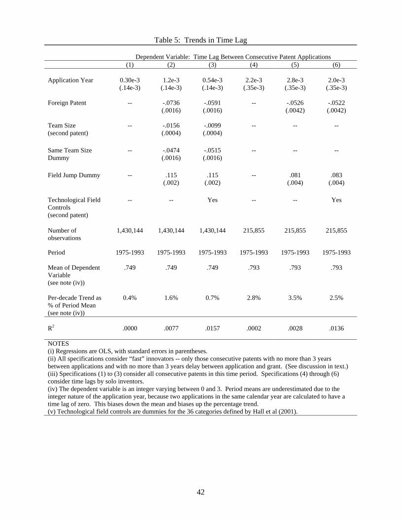
42

Table 5: Trends in Time Lag

Dependent Variable: Time Lag Between Consecutive Patent Applications (1) (2) (3) (4) (5) (6)

Application Year

0.30e-3 (.14e-3)

1.2e-3

(.14e-3)

0.54e-3 (.14e-3)

2.2e-3

(.35e-3)

2.8e-3

(.35e-3)

2.0e-3

(.35e-3) Foreign Patent

--

-.0736 (.0016)

-.0591 (.0016)

--

-.0526 (.0042)

-.0522 (.0042)

Team Size (second patent)

--

-.0156 (.0004)

-.0099 (.0004)

--

--

--

Same Team Size Dummy

--

-.0474 (.0016)

-.0515 (.0016)

--

--

--

Field Jump Dummy

--

.115

(.002)

.115

(.002)

--

.081

(.004)

.083

(.004) Technological Field Controls (second patent)

--

--

Yes

--

--

Yes

Number of observations

1,430,144

1,430,144

1,430,144

215,855

215,855

215,855

Period

1975-1993 1975-1993 1975-1993 1975-1993 1975-1993 1975-1993

Mean of Dependent Variable (see note (iv))

.749 .749 .749 .793 .793 .793

Per-decade Trend as % of Period Mean (see note (iv))

0.4%

1.6%

0.7%

2.8%

3.5%

2.5%

R2

.0000

.0077

.0157

.0002

.0028

.0136

NOTES (i) Regressions are OLS, with standard errors in parentheses. (ii) All specifications consider “fast” innovators -- only those consecutive patents with no more than 3 years between applications and with no more than 3 years delay between application and grant. (See discussion in text.) (iii) Specifications (1) to (3) consider all consecutive patents in this time period. Specifications (4) through (6) consider time lags by solo inventors. (iv) The dependent variable is an integer varying between 0 and 3. Period means are underestimated due to the integer nature of the application year, because two applications in the same calendar year are calculated to have a time lag of zero. This biases down the mean and biases up the percentage trend. (v) Technological field controls are dummies for the 36 categories defined by Hall et al (2001).

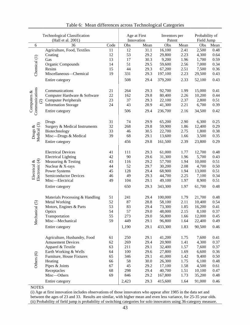
43

Table 6: Mean differences across Technological Categories

Technological Classification (Hall et al. 2001)

Age at First Innovation

Inventors per Patent

Probability of Field Jump

6 36 Code Obs Mean Obs Mean Obs Mean Agriculture, Food, Textiles 11 12 31.1 16,100 2.41 2,500 0.48 Coating 12 53 29.2 29,800 2.23 4,300 0.64 Gas 13 17 30.3 9,200 1.96 1,700 0.59 Organic Compounds 14 51 29.5 59,600 2.56 7,000 0.34 Resins 15 44 29.3 67,200 2.51 7,500 0.36 Miscellaneous—Chemical 19 331 29.3 197,100 2.23 29,500 0.43 C

hem

ical

(1)

Entire category 508 29.4 379,200 2.33 52,100 0.43 Communications 21 264 29.3 92,700 1.99 15,000 0.41 Computer Hardware & Software 22 162 29.8 80,400 2.26 10,200 0.44 Computer Peripherals 23 37 29.3 22,100 2.37 2,800 0.51 Information Storage 24 43 28.9 41,300 2.21 6,700 0.39 Entire category 506 29.4 236,700 2.16 34,500 0.42 C

ompu

ters

&

Com

mun

icat

ions

(2

)

Drugs 31 74 29.9 65,200 2.90 6,300 0.25 Surgery & Medical Instruments 32 268 29.8 59,900 1.86 12,400 0.29 Biotechnology 33 46 30.5 22,700 2.75 1,800 0.38 Misc—Drugs & Medical 39 68 29.1 13,600 1.66 3,500 0.35 D

rugs

&

Med

ical

(3)

Entire category 456 29.8 161,500 2.39 23,800 0.29

Electrical Devices 41 111 29.3 61,000 1.77 12,700 0.48 Electrical Lighting 42 90 29.6 31,300 1.96 5,700 0.43 Measuring & Testing 43 116 29.2 57,700 1.94 10,000 0.51 Nuclear & X-rays 44 52 29.7 30,200 2.08 4,700 0.50 Power Systems 45 128 29.4 68,900 1.94 13,000 0.51 Semiconductor Devices 46 49 29.3 44,700 2.25 7,100 0.34 Misc—Electrical 49 104 29.1 49,100 1.97 8,900 0.51 El

ectri

cal &

El

ectro

nic

(4)

Entire category 650 29.3 343,300 1.97 61,700 0.48

Materials Processing & Handling 51 241 29.4 100,000 1.79 21,700 0.48 Metal Working 52 87 28.8 58,100 2.11 10,400 0.54 Motors, Engines & Parts 53 83 29.4 73,300 1.85 16,200 0.41 Optics 54 57 29.0 48,000 2.15 8,100 0.37 Transportation 55 273 29.0 56,800 1.66 12,000 0.45 Misc—Mechanical 59 449 29.1 96,800 1.64 22,400 0.49

Mec

hani

cal (

5)

Entire category 1,190 29.1 433,300 1.83 90,500 0.46

Agriculture, Husbandry, Food 61 250 29.1 41,200 1.75 7,600 0.41 Amusement Devices 62 269 29.4 20,900 1.41 4,300 0.37 Apparel & Textile 63 211 29.1 32,400 1.57 7,600 0.37 Earth Working & Wells 64 100 29.6 27,800 1.69 6,600 0.36 Furniture, House Fixtures 65 346 29.1 41,000 1.42 9,400 0.50 Heating 66 58 30.0 26,300 1.75 6,100 0.48 Pipes & Joints 67 45 29.2 17,100 1.58 4,500 0.61 Receptacles 68 298 29.4 40,700 1.51 10,100 0.47 Misc—Others 69 846 29.2 167,800 1.73 35,200 0.48

Oth

ers (

6)

Entire category 2,423 29.3 415,600 1.64 91,000 0.46 NOTES (i) Age at first innovation includes observations of those innovators who appear after 1985 in the data set and between the ages of 23 and 33. Results are similar, with higher mean and even less variance, for 25-35 year olds. (ii) Probability of field jump is probability of switching categories for solo innovators using 36-category measure.

44

Table 7: Inventors per Patent vs. Tree Size

Dependent Variable: Inventors per Patent (1) (2) (3) (4) (5) (6) (7)

Normalized Variation in Tree Size

.0849

(.0010)

.0961

(.0010)

.0995

(.0011)

.120

(.001)

.133

(.001)

.107

(.001)

.152

(.001) Normalized Variation in Tree Size, Squared

.0609

(.0007)

.0545

(.0007)

.0545

(.0007)

.0341

(.0007)

.0257

(.0009)

.0356

(.0011)

.0404

(.0009) Foreign Patent

--

.446

(.002)

.442

(.002)

.420

(.002)

US Only

Foreign

Only

.371

(.003)

Normalized Variation in Direct Citations Made

-- -- -.0094 (.0011)

-- -- -- --

Technological Field Controls

--

--

--

Yes

Yes

Yes

Yes

Application Year Dummies

Yes Yes Yes Yes Yes Yes Yes

Number of observations

1,969,908

1,969,908

1,969,908

1,969,908

1,103,402

866,506

1,330,210

Period

1975- 1999

1975-1999

1975- 1999

1975-1999

1975-1999

1975-1999

1985-1999

Mean of Dependent Variable

2.02

2.02

2.02

2.02

1.82

2.27

2.13

R2

.026

.050

.050

.100

.090

.083

.079

NOTES (i) Regressions are OLS with standard errors in parentheses. Specifications (1) through (4) consider the entire universe of patents applied for between 1975 and 1999. Specification (5) and (6) consider separately patents from domestic vs. foreign sources. Specification (7) considers cross-sections from the later part of the time period. (ii) Normalized Variation in Tree Size is the deviation from the year mean tree size, divided by the year standard deviation in tree size. “Tree size” is the log of the number of nodes in the citations tree behind any patent. (iii) Normalized Variation in Direct Citations Made captures variation in the number of citations to prior art listed on a patent application. It is the deviation from the year mean number of citations, divided by the year standard deviation in the number of citations. (iv) Technological field controls include dummies for each of Hall et al.’s 36-category measure. (v) The number of observations here is slightly smaller than for the time trend analysis in Table 1 because a few patents do not cite other US patents, hence no citation tree can be built; these patents are dropped from the analysis.

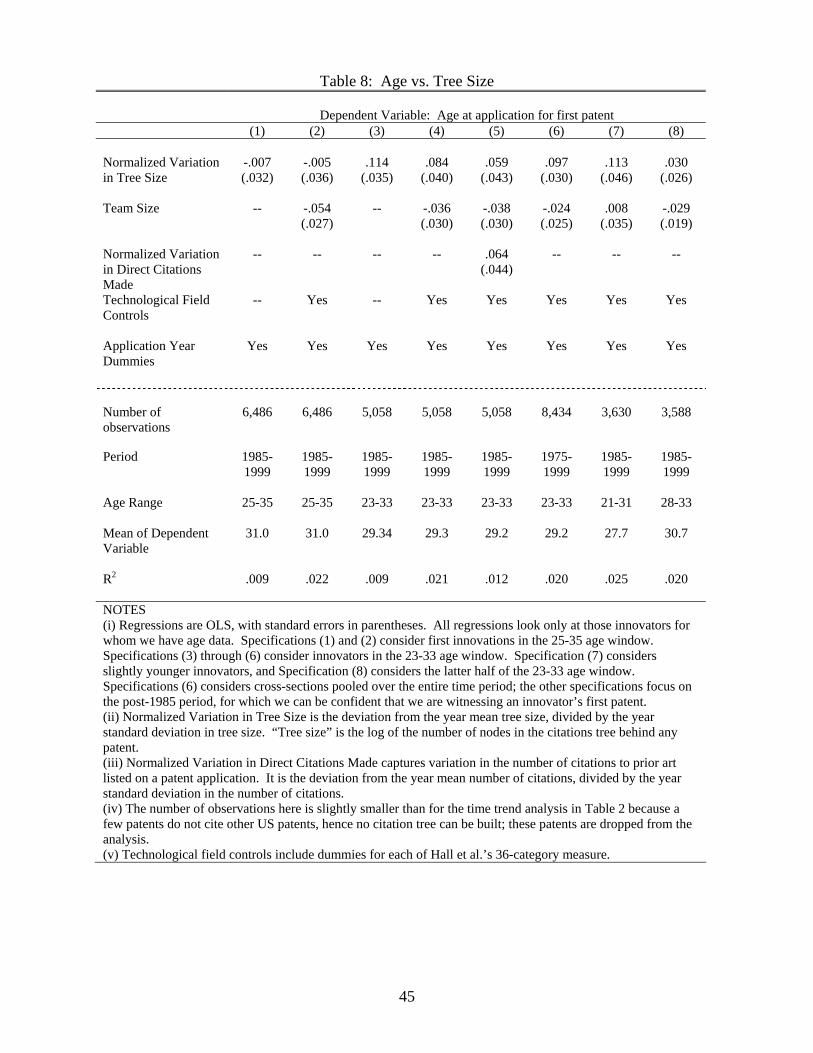
45

Table 8: Age vs. Tree Size

Dependent Variable: Age at application for first patent (1) (2) (3) (4) (5) (6) (7) (8)

Normalized Variation in Tree Size

-.007 (.032)

-.005 (.036)

.114

(.035)

.084

(.040)

.059

(.043)

.097

(.030)

.113

(.046)

.030

(.026)

Team Size

-- -.054 (.027)

-- -.036 (.030)

-.038 (.030)

-.024 (.025)

.008 (.035)

-.029 (.019)

Normalized Variation in Direct Citations Made

-- -- -- -- .064 (.044)

-- -- --

Technological Field Controls

-- Yes -- Yes Yes Yes Yes Yes

Application Year Dummies

Yes Yes Yes Yes Yes Yes Yes Yes

Number of observations

6,486

6,486

5,058

5,058

5,058

8,434

3,630

3,588

Period

1985-1999

1985-1999

1985-1999

1985-1999

1985-1999

1975-1999

1985-1999

1985-1999

Age Range 25-35 25-35 23-33 23-33 23-33 23-33 21-31 28-33 Mean of Dependent Variable

31.0

31.0

29.34

29.3

29.2

29.2

27.7

30.7

R2

.009

.022

.009

.021

.012

.020

.025

.020

NOTES (i) Regressions are OLS, with standard errors in parentheses. All regressions look only at those innovators for whom we have age data. Specifications (1) and (2) consider first innovations in the 25-35 age window. Specifications (3) through (6) consider innovators in the 23-33 age window. Specification (7) considers slightly younger innovators, and Specification (8) considers the latter half of the 23-33 age window. Specifications (6) considers cross-sections pooled over the entire time period; the other specifications focus on the post-1985 period, for which we can be confident that we are witnessing an innovator’s first patent. (ii) Normalized Variation in Tree Size is the deviation from the year mean tree size, divided by the year standard deviation in tree size. “Tree size” is the log of the number of nodes in the citations tree behind any patent. (iii) Normalized Variation in Direct Citations Made captures variation in the number of citations to prior art listed on a patent application. It is the deviation from the year mean number of citations, divided by the year standard deviation in the number of citations. (iv) The number of observations here is slightly smaller than for the time trend analysis in Table 2 because a few patents do not cite other US patents, hence no citation tree can be built; these patents are dropped from the analysis. (v) Technological field controls include dummies for each of Hall et al.’s 36-category measure.

46

Table 9: Field Jump vs. Tree Size

Dependent Variable: Probability of Switching Technological Field (1) (2) (3) (4) (5) (6)

Normalized Variation in Tree Size

-.0072 (.0008)

-.0074 (.0008)

-.0059 (.0008)

-.0095 (.0009)

-.0144 (.0012)

-.0184 (.0017)

Foreign Patent

-- -.0125 (.0018)

-.0108 (.0018)

-.0129 (.0018)

-.0135 (.0023)

.0032 (.0032)

Time Between Applications

-- -- .0226 (.0004)

.0232 (.0004)

.0215 (.0012)

.0143 (.0017)

Technological Field Controls (first patent)

--

--

--

Yes

Yes

Yes

Application Year Dummies

Yes

Yes

Yes

Yes

Yes

Yes

Number of observations

353,762

353,762

353,762

353,762

212,274

110,511

Period

1975-1999

1975-1999

1975-1999

1975-1999

1975-1993

1985-1993

Mean of Dependent Variable

.551

.551

.551

.551

.536

.520

(Pseudo) R2

.0039

.0039

.0117

.0251

.

.0171

.0159

NOTES (i) Results are for probit estimation, with coefficients reported at mean values and standard errors in parentheses. The coefficient for the Foreign dummy is reported over the 0-1 range. Only solo inventors are considered. Specifications (1) through (4) consider the entire set of solo inventors. Specification (5) considers only those solo inventors who meet the criteria in Specifications (1) through (6) in Table 3 (to help control for any truncation bias in the specialization measure – see the discussion of Table 3 in the text). Specification (6) considers the same data as Specification (5), but only looks at cross-sections in the later part of the time period. (ii) The dependent variable is 0 if an inventor does not switch fields between two consecutive innovations. The field is defined using the 414-category technological class definition of the USPTO. (iii) Normalized Variation in Tree Size is the deviation from the year mean tree size, divided by the year standard deviation in tree size. “Tree size” is the log of the number of nodes in the citations tree behind any patent. (iv) Technological field controls include dummies for each of Hall et al.’s 36-category measure.

47

Table A.1: Number of Observations at Each Stage of Selection

Number of

Observations

Percentage of

Row (3)

Percentage of

Row (4)

Percentage of Row Above

(1) Patents Granted

2,139,313

(2) Inventors Worldwide

4,301,229

(3) Unique Inventors Worldwide

1,411,842

(4) Unique Inventors with US Address

752,163 53.3% 53.3%

(5) Unique Inventors, US Address, Zip Code

224,152 15.9% 29.8% 29.8%

(6) Unique Inventors, US Address, Zip Code, Unique Match from AnyBirthday.com

56,281 4.0% 7.5% 25.1%

NOTES (i) Observation counts consider the 1975-1999 period. (ii) A “unique inventor” is defined by having same first name, last name, and middle initial.

Table A.2: The Assignment of Patent Rights Birth Data Assignment Status All

Patents US

Patents US Patents No zip code

US Patents Zip code

Direct Match

Other Patents

Unassigned

17.2%

22.4%

0.4%

98.3%

97.9%

26.6%

US non-govt organization

43.9% 72.9% 94.1% 0.0% 0.0% 65.7%

Non-US non-govt organization

36.2% 1.1% 1.4% 0.0% 0.0% 3.4%

Other assignment

2.7% 3.5% 4.1% 1.7% 2.1% 4.4%

NOTES (i) The first column considers all patent observations in the 1975-1999 period (2.1 million observations). (ii) US patents are those for which first inventor listed with the patent has a US address. (iii) The Birth Data columns consider those US patents with zip code information for which AnyBirthday.com produced a birth date. The first Birth Data column considers the specific patents on which AnyBirthday.com was able to match. The last column considers all other patents by that innovator, identifying the innovator by last name, first name, and middle initial. (iv) Unassigned patents are those for which the patent rights were still held by the original inventor(s) at the time the patent was granted; these patents may or may not have been assigned after the grant date. (v) Non-government organizations are mainly corporations but also include universities. (vi) Other assignment includes assignments to: (a) US individuals; (b) Non-US individuals; (c) the US government; and (d) non-US governments.

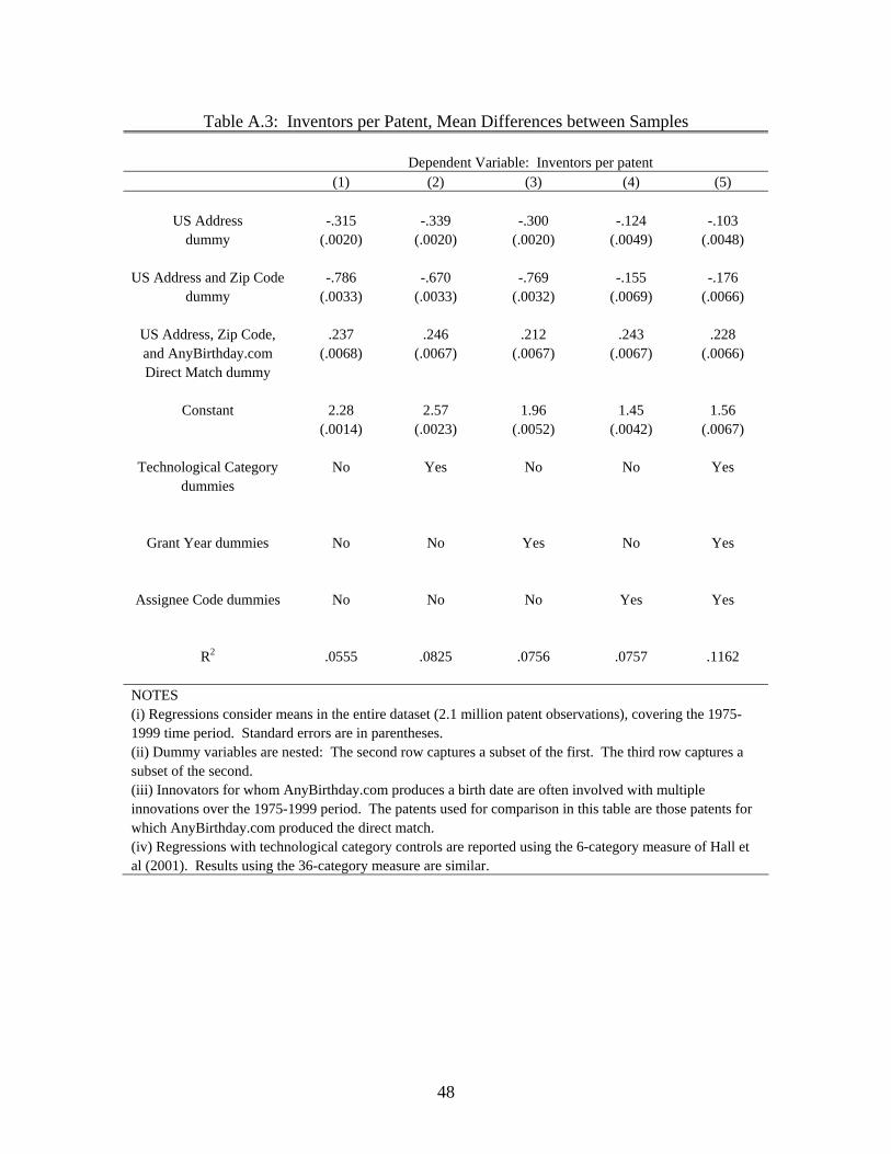
48

Table A.3: Inventors per Patent, Mean Differences between Samples

Dependent Variable: Inventors per patent (1) (2) (3) (4) (5)

US Address dummy

-.315

(.0020)

-.339

(.0020)

-.300

(.0020)

-.124

(.0049)

-.103

(.0048)

US Address and Zip Code dummy

-.786

(.0033)

-.670

(.0033)

-.769

(.0032)

-.155

(.0069)

-.176

(.0066)

US Address, Zip Code, and AnyBirthday.com Direct Match dummy

.237

(.0068)

.246

(.0067)

.212

(.0067)

.243

(.0067)

.228

(.0066)

Constant

2.28

(.0014)

2.57

(.0023)

1.96

(.0052)

1.45

(.0042)

1.56

(.0067)

Technological Category dummies

No

Yes

No

No

Yes

Grant Year dummies

No

No

Yes

No

Yes

Assignee Code dummies

No

No

No

Yes

Yes

R2

.0555

.0825

.0756

.0757

.1162

NOTES (i) Regressions consider means in the entire dataset (2.1 million patent observations), covering the 1975-1999 time period. Standard errors are in parentheses. (ii) Dummy variables are nested: The second row captures a subset of the first. The third row captures a subset of the second. (iii) Innovators for whom AnyBirthday.com produces a birth date are often involved with multiple innovations over the 1975-1999 period. The patents used for comparison in this table are those patents for which AnyBirthday.com produced the direct match. (iv) Regressions with technological category controls are reported using the 6-category measure of Hall et al (2001). Results using the 36-category measure are similar.

49

Ave

rage

Inve

ntor

s P

er P

aten

t Trends in Average Inventors Per Patent

Application Year1975 1979 1983 1987 1991 1995 1999

1.6 1.7 1.8 1.9

2 2.1 2.2 2.3 2.4

Age

Trend in Age at 'First Innovation'

Application Year1985 1987 1989 1991 1993 1995 1997 1999

30.5

30.8

31.1

31.4

31.7Ti

me

Lag

betw

een

App

licat

ions

Time Lag for 'Fast' Innovators

Application Year1975 1977 1979 1981 1983 1985 1987 1989 19911993

.65

.7

.75

.8

.85

Pro

babi

lity

of F

ield

Jum

p

Trend in Field Switch for 'Fast' Innovators

Application Year1975 1977 1979 1981 1983 1985 1987 1989 19911993

.51

.53

.55

.57

Figure 1: Basic Time Trends