Embed Size (px)
Citation preview

r//
NAVAL POSTGRADUATE SCHOOL_ Monterey, California
DTN7
THESIS
Incorporation and Comparative Evaluationof a Non-convective Cloud Parameterization
Scheme in the Naval Research LaboratoryWest Coast Mesoscale Weather
Prediction Model
by
Damacene V. Ferandez
June 1993
Thesis Advisor: Teddy R. Holt
Approved for public release;distribution is unlimited
93-27202• •'• • ~~.. .." • -;"• ~~lflllili1111HIll

UnclassifiedSECU RITY CL A SS;F -CAT O %J O( T-iS PA (]E
REPORT DOCUMENTATION PAGE 0ormo 0704o01
1a RFPOkrT E CURITY•.(ýAY F(AT;ON 0b RS."( T ./ VA¾•rUnc ias s iied
2a SECuRITY CLASSIFLAIION ALJIHORITY 3 D),STRriBjT
iON!AVAlA8,LITY o(F REPCJPT
2b DECLASSIFICATION, DOWNGRADING SCHEDULE- Approved for public release;distribution is unlimited
4 PERr )RMING ORGA.%:ZATiON REPORT NUMBER(S) 5 M().!TORITN( ORCANIZA 1O0 Ri Poi, '.'Mt-(M P(ý,
6a ._." 1E OF PERFORMING ORGANIZATION 6b OFFICE SYMBOL la NAME OF MONITORING ORGANZAT' )W(If applicable)
Naval Postgraduate School 35 Naval Postgraduate School
6c ADDRESS (City, State, and ZIP Code) 7b ADDRESS (City. State, and ZIP Code)
Monterey, CA 93943-5000 Monterey, CA 93943-5000
8a NAME OF IIJNDIr.G/SPONSOR'NG 1 b OFFICE SYMBOL 9 PROCUREMENT IIS'rPUIENT :DEN'I;t(A ()j,. %,.M t3EPORGANIZATION (if applicable)
8c. ADDRESS (City, State, and ZIP Code) 10 SOURCE OF iFjNDIrj(j NUMBERS
PROGRAM PROJECT TASK. 4ORK UNJITELEMENT NO NO NO ACCESSION NO
11 TITLE (Include Security Classification) INCURFORATPiON AND L UM"A=iVE tVA.UAi UN Ut ANON-CONVECTIVE CLOUD PARANETERIZATION SCHEME IN THE NAVAL PESEARCHLABORATORY WEST COAST MESOSCALE WEATHER PREDICTION MODEL12 PERSONAL AUTHOR(S) Damacene V. Ferandez
13a TYPE OF REPORT 13b TIME COVERED 14 DATE OF REPORT (Year, Month. Day) 15 PAGE COUNT
Master's Thesis FROM _ TO___ 1993 June 8416 SUPPLEMENTARY NOTATION The views expressed in this thes's are those of the
author and do not reflect the official policy or position of the Departmert
1 P" & COtAtI C •O . 1 -SUBJECRT ýEIRMS (Continue on reverse itf n(,cesjry and identity by block number)
FIELD GROUP SUB-GROUP
19 ABSTRACT (Continue on reverse if necessary and identify by block number)
This study describes the incorporation of the Sundqvist et al. (1989)explicit non-convective cloud liquid water scheme into the Naval ResearchLaboratory (NRL) limited area dynamical weather prediction model.Comparisons were made between model runs with the non-convective cloudwater scheme and those without the scheme to evaluate mesoscale windpattern, longwave radiation, temperature, and cloud simulations over theU.S. West Coast for the time period 0000 UTC 02 May 1990 to 1200 UTC 03May 1990. The most significant improvement in the updated model was themore physically realistic horizontal and vertical non-convective cloudstructures produced by the cloud liquid water fields.
20 DISTRIBUTION /AVAILABILITY OF ABSTRACT 21 &BST.ACT SE.CFVTYdLASSIFICATION
UNCLASSIFIED/UNLIMITED 0l SAME AS RPT El DTIC USERS nc assi ie22a NAME OF RESPONSIBLE INDIVIDUAL 22b TELEPHONE (Include Area Code) 22c OFFICE SYMBOL
T.R. Holt (408) 656-2861 MR/Ht
DD Form 1473, JUN 86 Previous editions are obsolete. SECURITY CLASSIFICATION OF THIS PAGE
S/N 0102-LF-014-o00i Unciassified

Approved for public release; distribution Is unlimited.
Incorporation and Comparative Evaluation of aNon-Convective Cloud Parameterization SchemeIn the Naval Research Laboratory West Coast
Mesoscale Weather Prediction Model
by
Damacene V. FerandezLieutenant Commander, United States Navy
B.S., U.S. Naval Academy, 1981
Submitted in partial fulfillment of therequirements for the degree of
MASTER OF SCIENCE IN METEOROLOGY
AND PHYSICAL OCEANOGRAPHY
from the
NAVAL POSTGRADUATE SCHOOLJune 1993
Author: 5 4
Damacene V. Fejadez
Approved by;_ _ _ _ _ _ _T.R Holt, Thesis Advisor
P.A. burkee, Second Reader
Robert L. Haneyf Chairman,Department of geteorology
ii

ABSTRACT
This study describes the incorporation of the Sundqvist
et al. (1989) explicit non-convective cloud liquid water
scheme into the Naval Research Laboratory (NRL) limited area
dynamical weather prediction model. Comparisons were made
between model runs with the non-convective cloud water
scheme and those without the scheme to evaluate mesoscale
wind pattern, longwave radiation, temperature, and cloud
simulations over the U.S. West Coast for the time period
0000 UTC 02 May 1990 to 1200 UTC 03 May 1990. The most
significant improvement in the updated model was the more
physically realistic horizontal and vertical non-convective
cloud structures produced by the cloud liquid water fields.
-J
looession For
Fi TS GRA&ITTIC TA ! El
jDist. CI Ds ... ,•~_ _

TABLE OF CONTENTS
I. INTRODUCTION .............. ................. 1
II. MODEL DESCRIPTION ............ .............. 3A. GRID .............. ................... 3B. EQUATIONS .............. ................. 9C. TIME INTEGRATION .......... ............ 10D. PARAMETERIZATIONS ..... ............ .. 11E. INPUT DATA .......... ............... 12
III. STRATIFORM PARAMETERIZATION .... ........ .. 13A. DESCRIPTION ....... ............... .. 13B. STRATIFORM CONDENSATION ............ .. 14
IV. WEATHER SCENARIO ....... .............. 24A. SYNOPTIC SITUATION ...... ........... 24B. MESOSCALE FEATURES ...... ........... 29
V. CONTROL MODEL SIMULATIONS .... .......... ..41A. CATALINA EDDY ....... .............. 41B. SOUTHERLY SURGE ....... ............. 43
VI. TEST MODEL RUN EVALUATIONS .... ......... .. 47A. MESOSCALE WIND FEATURES .... ......... .. 47B. CLOUD FRACTION ........ ............. 48C. LONGWAVE RADIATION ...... ........... 56D. TEMPERATURE ....... ............... .. 60E. CLOUD LIQUID WATER ...... ........... 64
VII. CONCLUSIONS AND RECOMMENDATIONS ......... .. 70A. CONCLUSIONS ........ ............... .. 70B. RECOMMENDATIONS ........ ............. 72
REFERENCES ............ ................... 74
INITIAL DISTRIBUTION LIST ..... ............ .. 76
iv
ACKNOWLEDGMENTS
I would like to thank Russ Schwanz for all his help with
my IDEA lab files and to Steve Drake for answering all of my
endless questions on the VISUAL display program. Thanks
also to Mark Boothe for always getting the last-minute
computer equipment I needed. My thanks to Professor Phil
Durkee for his welcome suggestions and review of this
thesis. Finally, my sincerest gratitude to Professor Teddy
Holt for his continued patience, support, and guidance
during this study and throughout my time at NPS.
This research was funded by the NPS Direct Merit
Funding.
V

1. INTRODUCTION
The Naval Research Laboratory (NRL) Limited Area
Dynamical Weather Prediction Model is an evolving research
model for testing new methods of modeling various mesoscale
phenomena. The model has shown success in resolving
topographic and coastal features. Also, high vertical
resolution in the lower levels of the model has allowed
close examination of processes occurring within the boundary
layer. Previous studies (Grandau 1992 and Stewart 1992)
have demonstrated the NRL model's effectiveness in resolving
mesoscale and boundary layer features in this region.
The United States West Coast poses a big modeling
challenge due to its topographic features and coastal
mesoscale phenomena such as the Catalina eddy and the
southerly surge. In addition, much of the California coast
experiences frequent stratus clouds which can significantly
affect the weather in the region.
The stratiform condensation (or non-convective) process
is important in modeling coastal mesoscale phenomena. A
very simplistic approach is to represent cloud cover as
being either total or zero for each grid box depending on
whether gridpoint relative humidity has reached 100% or not.
A more advanced technique would be to parameterize the
process on the subgrid scale. Cloud cover (or cloud
1

tract ion) c (ou Id be (Aeterrmi ned more realistically as a
function of gridpoint relative humidity and a relative
humidity threshold or critical value.
This study examines the incorporation of the stratiform
condensation process of Sundqvist et al. (1989) into the NRL
limited area mesoscale model. Previous NRL model
simulations by Stewart (1992) included cloud fractions as
determined by the method of Slingo and Ritter (1985) . These
simulations, hereafter referred to as the "control" case,
will be compared to the NRL model incorporating the
Sundqvist et al. explicit non-convective clouid liquid water
scheme, hereafter referred to as the "test" case. The
inclusion of cloud water as a variable in predicting
stratiform clouds is a major feature of Sundqvist's scheme.
Section II describes the NRL mesoscale model and the
extent of the geographic region involved. Section III
outlines the Sundqvist et al. stratiform parameterization
technique. Section IV is the regional weather scenario for
the time period including specific mesoscale phenomena.
Section V describes the mesoscale structure of the control
model simulations. Section VI evaluates the test model runs
in comparison to the control model, and Section VII includes
conclusions and recommendations.
2

II. MODEL DESCRIPTION
The Naval Research Laboratory (NRL) regional weather
prediction model is a quasi-hydrostatic, baroclinic,
mesoscale model which incorporates cumulus, boundary layer,
and radiation parameterizations. This limited area model is
most appropriate where near-gradient balance of large scale
motions in the lower troposphere exists.
Since the isobaric coordinate system does not easily
handle varying topography, the vertical coordinate sigma (a)
is used. This is defined as the ratio of pressure to the
surface pressure.
T= ( ) (2.1)PO
Specifics of the NRL model are detailed by Madala et al.
(1987) . The basics are outlined in the following pages.
A. GRID-
The horizontal grid is a staggered Arakawa C-grid. This
type of network is best for the simulation of wind field
geostrophic adjustment and conservation of integral
properties. General curvilinear horizontal coordinates with
user specified horizontal grid spacing is used. For an M X
N field (i=1,2,...M; j=1,2,...N), temperature (T),
3

geopotentlal height ON), specific humidity (q), and sigma
(a) are computed at mass points (1,) with u-velocity
(east-west) and v-velocity (north-south) computed at the
midpoints along the :a- ind y-axis respectively (See F-.gure
1).
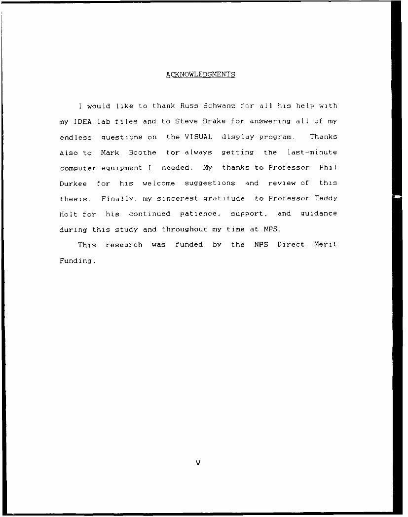
The horizontal domain is a 103 X 91 grid with 1/6 degree
resolution in latitude and longitude from 20 N to 43' N and
113iW to 130 W. Figure 2A shows the extent of this region
along with points of interest referred to for profile and
cross-sectional plots in this study and Figure 2B Ilisplays
main geographic points of reference. Mode! simulations
employ 23 vertical sigma levels as shown in Table 1.
Thirteen of these layers are below 850 mb ensuring a high
vertical resolution within the boundary layer.
4

I I
IauI I 6: V , ,
Ii
I I
0'*
o ~y
Figure 1Horizontal and vertical grid networkittilized In the NRL mesoscale model
(Madaia et al. 1997)
5
I
L..............-------........35 -.. -----..................... - ,i.. .... .. . ......... -i
\ iL
0. ...................... --..... ............. -----...... . .....................
-ZO ii
Point 'A' (35N,121W)Point 'B' (33N,122W)Point 'C' (30N.127W)Point 'D' (34N,119W)
Figure 2ANRL model horizontal domain.
6

San Franclsco
Bay
Monterey Bay
San Simeon
35 - • .. . . . . . . . . . . . .......... S a n L u i s~a O b i s p o - . . . .. . . . .. . . . . . . . . . .. . . . . . . . . .
SnBay
:, :Santa Barbara
Pt Conception '-'-
"--Los Angeles
Santa CruzIsland It
Santa Catalina r\Island
San Diego
125 12O
Figure 2BSignificant geographic points.
7

TABLE 1MODEL SIGMA LEVELS
Model Level Sigma (e)
1 0.05
2 0.15
3 0.25
4 0.35
5 0.45
6 0.55
7 0.64
8 0.715
9 0.78
10 0.835
11 0.88
12 0.915
13 0.94
14 0.957
15 0.969
16 0.978
17 0.985
18 0.99
19 0. 9935
20 0.996
21 0.99775
22 0.998
23 0.99975
8

B. EQUATIONS-
The governing primitive equations are formulated in
surface pressure flux forms (i.e. p, u p v, etc.). The
dynamic system consists of seven equations, five of which
are prognostic, and two which are diagnostic. (See Madala.
1987 for the complete form of the equations).
u- & v-momentum equations:
a (p,u) (2.2)
a (P.V) (2.3)d t
thermodynamic equation:
a (P'7 (2.4)
moisture continuity equation:
S(pgq) (2.5)at
surface pressure tendency equation:
(p,) ((2.6)at
9

hydrostatic equation:
S(2 .7,
continuity equations:
a1 (P.6) (2.8)aT
A closed system is formed for the dependent variables u, v,
T. q, p, , P, and b (vertical velocity)
C. TIME INTEGRATION-
The split-explicit method is utilized which effectively
splits terms in the prognostic equations into two parts:
those governing the Rossby modes and those governing the
faster gravity modes. For quasi-linear gravity modes, the
pressure gradient and divergence terms vary taster than the
remaining terms. This allows that part of the equation with
these remaining terms to use a larger time step. The split
equations are integrated with time steps for their
respective CFL criteria.
10

D. PARAMETERIZATIONS-
The model parameterizes a number of physical processes
including cumulus precipitation, planetary boundary layer
(PBL) processes, and radiation.
Cumulus parameterization is from the modified Kuo scheme
(Kuo 1974) . Surface layer parameterization is based on
Monin-Obukhov similarity theory. PBL parameterization is
with turbulent kinetic energy (TKE) closure described in
Holt and Raman (1988).
The radiation parameterization incorporated in the model
is the Harshvardhan et al. (1987) scheme. Stewart's (1992)
study parameterizing longwave and shortwave effects showed
the improvements in the model's ability to simulate diurnal
and cloud-related radiative processes.
The cloud parameterization scheme incorporated in the
con, ol model by Stewart (1992) is based on cloud fractions
using a modified Slingo and Ritter (1985) method where
average layer relative humidities are compared to critical
relative humidity values. This method produces stable and
convective cloud fractions for a horizontal grid at each
sigma layer. The clouds are diagnosed as either stratiform
or cumulus.
Due to the frequent presence of stratiform clouds along
the west coast, the need for a more sophisticated non-
convective parameterization scheme is clear. This
11

strat iform parameterl zat 1n io 1 discussed 1n cietala i n
Section III.
E. INPUT DATA-
Data for the period 0000 UTC 02 May - 1200 UTC 03 May
1990 was taken from the Navy Operational Global Atmospheric
Prediction System (NOGAPS). Model initialization data was
retrieved from archived Fleet Numerical Oceanography
Center's 2.5 degree global analyses and horizontally and
vertically interpolated to the NRL model resolution (Grandau
1992). Fields include u- and v- components of velocity,
temperature (T), vapor pressure, sea level pressure, and sea
surface temperature (SST).
12

III. STRATIFORM PARAMETERIZATION
A. DESCRIPTION-
Increased development of mesoscale atmospheric modeling
has resulted in a more involved look at the proper treatment
of the stratiform condensation process. The high occurrence
of stratus clouds along the U.S. West Coast and its effect
on regional weather patterns makes this region ideal for
this type of study.
One assumption typically made in representing stratiform
condensation is that the gridpoint relative humidity must
reach 100% in order for condensation to occur. This results
in a simplistic approach of cloud cover either being
represented as zero or 100% at individual grid points. A
more realistic treatment of this case would be a subgrid
scale method requiring a parameterization of the process.
Sundqvist et al. (1989) devised a treatment of
condensation cloud processes for convective and non-
convective precipitation. This study will only incorporate
Sundqvist's non-convective scheme. The convective case
utilizes the scheme by Kuo (1974) adopted to account for the
inclusion of cloud water as a prognostic variable. The
13

first step in the parameterization of convective and non-
convective precipitation is a stability check of the grid
column. The criterion here is that an air parcel at the
surface shouid be positively buoyant after reaching the
lifting condensation level (LCL). If the column is
conditionally unstable, the Kuo scheme (without Sundqvist's
modifications) is used. If not, the possibility of
stratiform condensation is investigated. The Sundqvist et
al. stratiform condensation treatment is described in the
following pages.
B. STRATIFORM CONDENSATION-
For stratiform condensation to take place, a relative
humidity threshold value (of less than unity) within a grid
box must be exceeded. Parameterization of the stratiform
condensation process is a function of quantities such as
stability, cloudiness, altitude, and type of surface. The
prognostic equations used are those for cloud water mixing
ratio (m), temperature MT), and specific humidity (q).
Changes in cloud water are due to local changes in m
from advection and diffusion (A .), latent heat release (Q),
local rate of release of precipitation (P), and evaporation
14
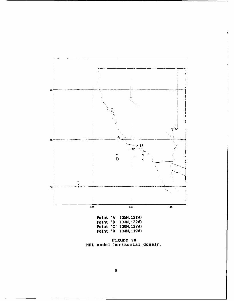
of cloud water to vapor advected to a grid box where no
condensation is occurring (E,). In equation form,
-r Am+Q-P-Ec (3.1)
where Omn/at is total cloud water mixing ratio tendency.
The local rate of release of precipitation (P) is dependent
upon a cloud liquid water threshold value (m,). Efficient
release of precipitation occurs when m exceeds the cloud
fraction multiplied by this threshold value.
P-cm[lie-e ( * ]) (3.2)
c. is characteristic conversion rate of cloud
particles to precipitation size, and
b is the cloud fraction.
The cloud fraction is determined from the relative
humidity (RH), a relative humidity threshold value for
condensation (RHc), and the weighted average of the humidity
of the cloudy part (RH.). (RH. is defined to equal the
value of 1).
b=1- (Rug-Pi-n (3.3)15(RK 5 _c)
I1

Typically, RHC values are empirically derived. Sundqvist
et al. (1989) used RH threshold values above the boundary
layer of:
0.75 -- over land, and
0.85 -- over the ocean.
In the boundary layer, RW is assumed to linearly
approach unity at the surface. Subgrid-scale topography
effects are taken into account by assuming the value of Rl
to be 0.1 lower over the land than over the ocean. Also, to
prevent the unrealistically early formation of cirrus
clouds, RH, is increased asymptotically toward unity for
temperatures less than 2380 K. Figure 3 depicts the
Sundqvist et al. relative humidity threshold profile.
This is contrasted with the approach by Slingo and
Ritter (1985) and used by Stewart (1992) in the control
model simulations. Here, different critical relative
humidity values are computed as a function of sigma. For
each model sigma level, a critical relative humidity is
determined from the equation:
RHC=I+2(o2-o)÷1/r3•(i-3o+2a2) (3.4)
In order to account for the lack of model-simulated
clouds near the coastal regions, Stewart used satellite
imagery to propose a modification of critical relative
humidity values for this particular 2-3 May 1990 case study.
16

OVER
T 2 & LAND *
I /OVEROvA E R
I
-.. ... ........... ...... ------------ -----------------------
Bounder yLayef
Iyo
70% 80% 90% 100%
Critical Relative Humidity (RHd
Figure 3Critical Relative Humidity Profiles
(Sundqvlst et al, 1g89)
17

Figure 4 shows the representations of critical relative
humidity values by both Slingo et al. and Stewart.
For stratitorm clouds, the evaporation of precipitating
water to vapor as it tails through subsaturated air kE,)
depends on cloud fraction (b), relative humidity (RH) , and a
layer-averaged precipitation rate (0).
E,=k,(RH,-aR) (i-b)rP (3.5)
k, is a coefficient expressing the instantaneous evaporation
of advected m.
Temperature changes are due to the temperature tendency
from advection, diffusion, and radiation (A,), latent heat
release (Q), evaporation of precipitating water to vapor
(E,) , and evaporation of advected cloud liquid water (Ec).
aT=A (-L L (Ec+Er) (3.6)
cP in this equation is the specific heat of dry air at
constant pressure, and L is latent heat of vaporization.
The change in specific humidity (aq/at) comes from the
effects of advection and diffusion (A,), latent heat release
(Q). and evaporation (E,+E,).
a'=Aq-QEc÷Er (3.7)
18

0
0.2
0.4
E0.6
0.8
1.040 50 60 70 80 90 100
Critical RH (%)
Figure 4Critical relative humidity profiles.
(Slingo & RItter -- solid)(Stewart -- dashed)
(Stewart 1992)
19

Combining the prognostic equations ror temperature and
specitic humidity with the ilausius-Clapeyron equation
(Sundqvist L988) qives an expression tor r
M-q[ a(RH) I
1+ (RH)eL 2q, 38)
RcPT2
where M is the convergence of available latent heat given
as:
M=Aq (RH)eLq, (AT) + (R ( q, ] S)( 3.9)RT 2 (A)+ P at
q. is saturation specific humidity.
e is the ratio of molecular weight of vapor
to molecular weight of dry air (=0.622), and
R is the gas constant for dry air.
Hence, positive advection of A, and pressure tendency
(ap/at) would tend to increase available latent heat
convergence, while warm advection (A , > 0) would tend to
decrease convergence.
To close the system, the tendency of RH can be expressed
by:
a(RH) _ 2 (1-b) (RPHf-RHf) [ (1-b)M+E1 ]
at 2q,-(1b) (RH.-RHc) +÷( ) (3.10)
b
At this point, temperature and specific humidity
tendencies (aT/at and aq/a) can be computed. The mixing
20

ratio tendency (din/at) is obtained by semi-implicit time
integration of equation (3.1), which may be rewritten as:
-a=RHS-P (3.11)
---- =--HS-cM [ 1 - e _(._) (3.12)
(RHS = right hand side)
And in finite difference form:
_(• )a(3.13)mn+1=mn-1÷2A t (RHS) -2A tc•[l1-e(3
T=rn-! (Mn2+1 }+MDl) (3.14)2
Resulting in a non-linear equation,
x[I+A tco(l-e-a) ]=m'2-1+ (RHJS) A t (3.14)bm,
m. r (3.15)
which may be solved using the Newton-Raphson iteration
method.
Table 2 provides a summary of various stratiform
condensation processes described by the tendency equations
and their influences. Water vapor condensing into cloud
21

TABLE 2SUMMARY OF STRATIFORM CONDENSATION PROCESSES
I .gPPflprn "HIMIUIfTY' T;AnDMfNh'~
t : A4- 0 + E0+ E,
[TAJPFRATD1R~ rFNnFNtir
'' - T 0o - o 0
A= 0 - E
PROCESS SIGNIFIOANT___________ TERM q.T.m TENDENCY
S
q condenses Q :ql TI mlto m *uve
m
m advected & :
evaporatestoq E0 q TI Ml,I .1
precipitationevaporates Er qi T m.
to qSI A.
m precipitates p q- T- -- mjout
22

liquid water results in a decrease in specific humidity (q),
and an increase in temperature (T) and cloud liquid water
(m). When cloud water is advected and evaporated into water
vapor, specific humidity is increased, while temperature and
cloud liquid water are decreased. For the case where
precipitation evaporates to vapor, specific humidity is
increased and temperature is decreased. Finally, for cloud
water precipitating out, cloud liquid water decreases, with
specific humidity and temperature remaining constant.
23

IV. WEATHER SCENARIO
A. SYNOPTIC SITUATION:
1. Upper Air-
The period of interest for this study is 0000 UTC 02
May 1990 to 1200 UTC 03 May 1990. A high pressure ridge
dominated the eastern Pacific region and slowly intensified
during the period. A closed upper level low that was
situated over southern Arizona initially deepened and
subsequently filled and moved eastward over the latter part
of the period.
There was also evidence of a weak shortwave moving
over the Pacific Northwest at the start of the period.
Figures 5A to 5D show the 500 mb pattern for the period.
2. Surface-
During this period, a weak low pressure area
originating in the north central Pacific deepened and moved
to the northeast. This low pressure cell eventually reached
the British Columbia coast at the end of the period.
A closed high pressure cell was located in the
eastern Pacific off the northern California coast ridging
24

O0 UTC 2 May 1990NOGAPS 500 mb
50 I• --
It•
40 -• i I.. __. 5640
,+.,+30 , • /
150 140 130 120 110 100LONG (°W)
Plgu.re 5A0000 UTC 02 May 1990
NOGAPS 500 mb Analyslshei9hts (solid, l)
LeIperature (dashed, °C)
O0 UTC 2 May 1990NOGAPS Sea level pressure (mb)
+ : f
| I
•o ,• __j •)\ \• "•
20 ! t-•150 140 130 120 + 10 100
LONG (°W)
Ffgure 6A0000 UTC 02 Hay 1990
NO.GAPS Sea Level Pressure Analysls
25

12 UTC 2 May 1990NOGAPS 500 mb
50
IL-
-530
20150 140 130 120 110 100
LONG (0W)Figure 58
1200 UTC 02 May 1990NOGAPS 500 mb AnalysIs
heights (solid, m)temperature (dashed, 00)
NOGAPSSea level pressure (mb)50
40
104 -1
30NN
20150 140 130 120 110 100
LONG (WFigure 6B
1200 UTC 02 May 1990NOGAPS Sea Level Pressure Analysis
26

00 UTC 3 May 199050 AP 00m
40V 4
300
200
150 140 130 120 110 100LONG (0WM
Figure 5C0000 LJTC 03 May 1990
NOGAPS 500 mb Analysisheights (solid, a)
temperature (dashed, 0C)
00OUTC 3 My 1990NOGAPSSea level pressure (mb)
50 IA
30U
150 140 130 120 110 100* ~LONG (0W
Figure 6C0000 UTC 03 May 1990
NOGAPS Sea Level Pressure Analysis
27

soNOGAPS 50m
40
150 140 130 12'0 110 100LONG (OW)
Figure 5D1200 UTC 03 May 1990
NOGAPS 500 mb Analysisheights (solid, a)
temperature (dashed, 00)
12 UrC3 May 1990NOGAPSSea level pressure (mb)
150 10 13 12 11 10
28
into the Pacific Northwest. The high pressure pattern
continually weakened while gradually moving northeastward
toward the Washington coast.
A thermal low remained over Arizona and filled
slightly during the period. This low had an associated
inverted trough extending over the California coast. (See
Figures 6A to 6D).
B. MESOSCALE FEATURES:
Specific mesoscale features of interest for the region
during the period include the land and sea breeze, the
Catalina eddy, and the southerly stratus surge. Satellite
images show a dominant presence of stratus along the
coastlines during this time period. Because of the close
association of stratus clouds with the latter two features,
this study concentrates on the Catalina eddy and the
southerly surge.
1. Catalina Eddy-
The Catalina eddy is a feature typically occurring
from late spring to early fall characterized by surface wind
cyclonic circulation in the vicinity of Santa Catalina
Island. Figure 7, from Mass et al. (1989), is a Catalina
eddy composite of 1200 UTC surface winds (knots) and sea
29

S 04 LST 04 LSTCATALINA EDDY 1012.9 1.4
;1010.4CLM
1010.3 101 .7
,•0.4
110.0 " 10-12.2.1010. 101012.8'
Figure 71200 UTC Catalina Eddy and climatologycomposite of surface winds (knots) and
sea level pressure (millibars).
(Catalina eddy composite based on 50 events;climatology composite based on data for Maythrough September 1964-1982)
(Mass and Albright, 1989)
30
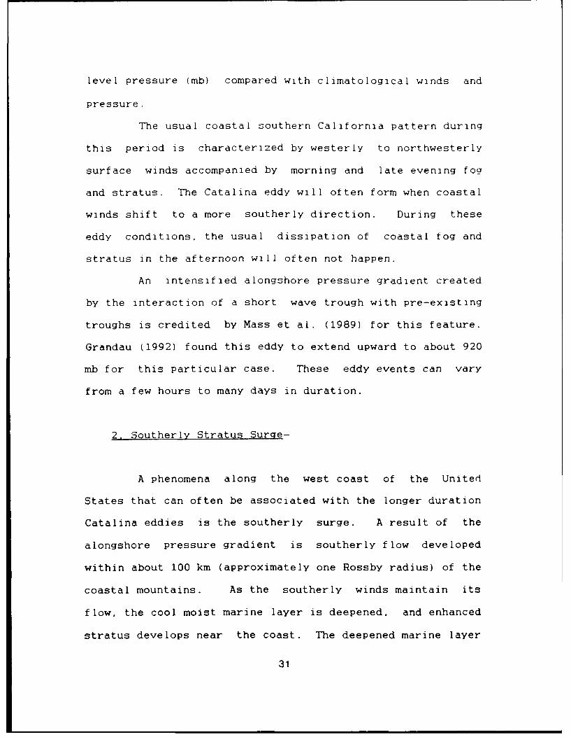
level pressure (mb) compared with climatological winds and
pressure.
The usual coastal southern California pattern during
this period is characterized by westerly to northwesterly
surface winds accompanied by morning and late evening fog
and stratus. The Catalina eddy will often form when coastal
winds shift to a more southerly direction. During these
eddy conditions, the usual dissipation of coastal fog and
stratus in the afternoon will often not happen.
An intensified alongshore pressure gradient created
by the interaction of a short wave trough with pre-existing
troughs is credited by Mass et al. (1989) for this feature.
Grandau (1992) found this eddy to extend upward to about 920
mb for this particular case. These eddy events can vary
from a few hours to many days in duration.
2. Southerly Stratus Surge-
A phenomena along the west coast of the United
States that can often be associated with the longer duration
Catalina eddies is the southerly surge. A result of the
alongshore pressure gradient is southerly flow developed
within about 100 km (approximately one Rossby radius) of the
coastal mountains. As the southerly winds maintain its
flow, the cool moist marine layer is deepened, and enhanced
stratus develops near the coast. The deepened marine layer
31

will often result in improved air quality ror the Los
Angeles area.
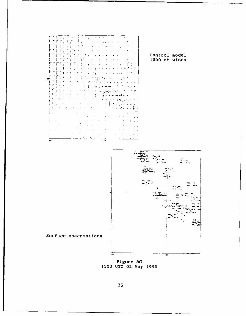
Figures HA through 8G include burtace wind
observations for the period of interest. Corkill (1991)
described a weak southerly surge for his study covering the
same time period. Figure BF shows southerly coastal winds
from central to southern California at 2100 UTC 02 May 1990.
The 2030 UTC visible satellite image (Figure 9) reveals
coastal cloudiness all along the central California coast
from Monterey to San Luis ubispo Bay. Dorman (1985)
described the southerly surge as a result of coastally-
trapped gravity currents, while Mass et al. (1989) stated
that it results from a coastally trapped two-layer marine
system.
32

rrr r f- rrrrvri: --,. ... .. .,rm i r .. Control modelF f "..... ... 1000 mb winds
r r f- ', t* . . . . . ,
I- • t K ,K r.- .' •/ r
S. . .. . ' • • + • " - , --r --"r °
.. . . (Wind speed in knots.
.. [short barb 5 knots][long barb 10 knots]
• --.,,,
Surface observations
Figure 8A0900 UTC 02 May 1990
33

".. " , Control modelS.... r. r ** 1000 mb windsI- t ' t- +• '..........rr
ST •,[ '.rr......•
*' + ,. i . -. ..
a -a - ---- .- ..--.S. . . < z a .£ -.• • £ • . •
.a. I' ,.
• • •-:.,-,. ..-
4J6
34,,.,,, 1++. .. ..
o.S , - a" p
Surface observations
Figure 8B1200 UTC 02 May 1990
34
,r I~ -r . !.' i' r
Vr r-r i r - ' I .. . -, ."I I-F F F r ." . . ........ Control model
F FF r-FF " ... . . . . . . .. . "1000 mb winds7 F -' F I- r .. . . .. . . .. -' .
r rr F .. . .. .F
• ,,:..• L.1_-, ,,--, • '
. . . .. . . .. . . .
.. .... r-..
S.e.
Surface observations
Figure 8C1500 UTC 02 May 1990
35

"F C- . .Control model"1000 mb winds
• I- r F I . .. . . . . .. . . .
YF F r"F F I i ~ . -. t-.'' . .. ,.
i \ , •. . .r
......... .. .
-.. .- * ° ° °
. , ,v..\,
Surface observations
Figure 8D1800 UTC 02 May 1990
36
= e

in n
. .Control modelS. ... ... . .1000 mb winds
*.... ,. ..... .... ... _
. . .. .. . . ._ . L .. ., _
\ , \. . .. , •. a . _
IZ, 20
"" F>
Surfacegur obevain
2100 UTC 02 May 1990
37

, . ." t Control modelF 1 -1 r 1000 mb winds
r rrr
~~A6-•-...............
~\ .4.....
'. ,, •
( ... 4.. .....4
• '', • . -:" ,
Surface observations
FIgure 8F0600 UTC 03 May 1990
38

-r r.
"rI' /- r • Control model
r, r . .. f- 1000 mb winds,rrrrr \rr tr .
rr, r . . .. .
\. -*_•. L _•L.J. .-
4" . . 4. . L 4.L. ** _ •
Surface observations
Figure 8G1200 UTC 03 May 199o
39

-o -
20"1(03 UTM-0C 02; May 90)
pp" _7 -.- ;40

V. CONTROL MODEL SIMULATIONS
Stewart (1992) incorporated the Harshvardhan et al.
(1987) radiation parameterization into the NRL regional
weather prediction model and conducted model simulations
integrated for 36 hours over the time period 0000 UTC 02 May
to 1200 UTC 03 May 1990. Integration over the same area and
time window allows for consistent comparisons with the
control model of Stewart to evaluate the impact of the new
stratus parameterization.
A. CATALINA EDDY-
The control model low-level wind fields (Figures 8A to
8G) indicated clear onset of a Catalina eddy at 0900 UTC 02
May 1990 with south-southeasterly winds near San Diego and
clear off-shore flow along the central to southern
California coast. Further off the coast, general northerly
winds were observed off Monterey Bay to west-northwesterly
flow toward the Mexico border.
Three hours later, the model clearly defined the eddy
pattern in the Los Angeles basin with the vortex centered
between the Santa Cruz and the Santa Catalina Islands. By
1800 UTC, the pattern had become disorganized with a
41

transition or southerly winds extending along the cOast fromn
San Simeon to Santa Barbara.
At 2100 UTC, the winds are westerly from Pt. Conception
northward, and from the southwest in the Los Angeles basin.
By 0600 UTC, another eddy onset appeared to be occurring,
with the 1200 UJTC wind fields again giving a clear eddy
pattern.
Comparison of model-predicted wind fields and a limited
number of land and ship observations showed that the
Catalina eddy onset appeared to be reasonably predicted.
However, the model seemed to show the dissociation of the
eddy sooner than the observations indicated. The 1800 UTC
reports still show evidence of an eddy circulation, while
the model showed mostly onshore winds along the coast.
Also, observations near San Diego showed the winds
maintaining more of a southerly component longer into the
period (through 0600 UTC 03 May). Because of the lack of
data, the reformation of another eddy later by 0600 UTC
could not be readily verified.
42
B. SOUTHERLY SURGE-
The control model low-level wind fields (Figures 8A Lo
8G) showed distinct southerly coastal wind flow from San
Simeon to San Diego at 1800 UTC 02 May 1990. By 2100 UTC,
winds from San Simeon to Santa Barbara shifted to a
predominantly western direction. From 0000 UTC 03 May 1990,
winds in the area had prominent northerly components.
Observations along the coast showed southerly wind flow
from Santa Barbara southward at 1800 UTC 02 May 1990.
Coastal areas to the north however did not have southerly
winds until 2100 UTC 02 May 1990. This coastal southerly
wind flow continued up to the end of the period.
Coincident with the southerly surge time period,
satellite imagery showed persistent cloudiness along the
coastline from Monterey Bay to San Luis Obispo Bay. The
normal late day coastal fog and stratus dissipation occurred
only to the south. Persistent coastal fog and stratus with
little dissipation is expected during a southerly surge
stage. Figure 9 is a visible satellite image highlighting
the coastal cloudiness for the region.
Time-height cross-sections for point 'A' near San Luis
Obispo Bay (35°N, 121'W) showed model southerly winds near
the surface at around 1800 UTC 02 May time period. Figure
10 shows the southerly surface flow isolated during that
time window (dashed lines indicate northerly winds while
43

ii
. .
\
a a
ax- -N N -\- - -
Nl \ 1 - - # - N
N - - Nt iI I I 1
II z \
'I A / - S I I 14
S/ / /\ I
I N/I I
I I I I I 11 t |I SI I
i i I I / N/ - \ i I 1,,I; / I I SI I I
II_. : I-- - , , -. .
I .oii 'II 2 I 2 ' , ' .. Ii, IIII,:
0 3 6 • 2 L 118 21 2• 27 30 33 38
Figure 10Control model time-height cross-section of
southerly (v-component) winds (m/s) at Point 'A'.
44
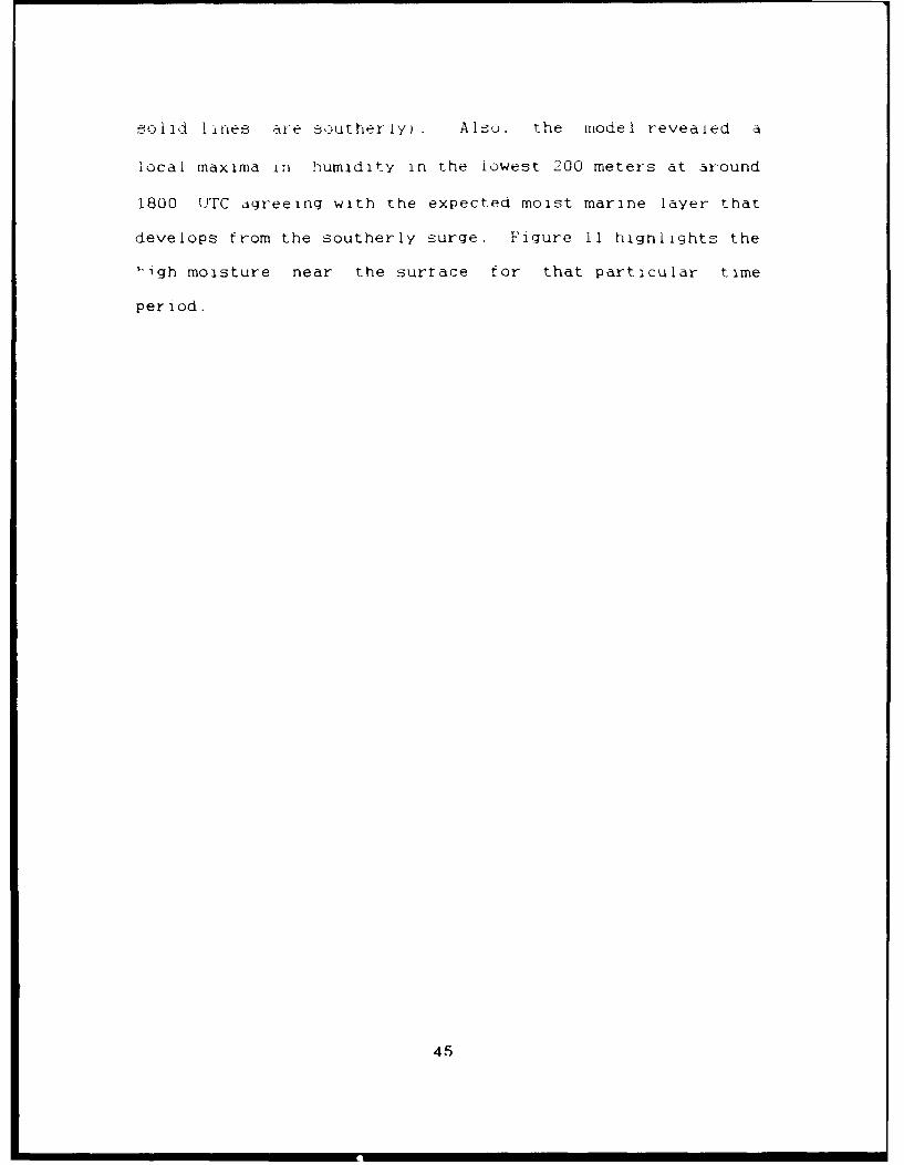
•O lid I a-e aze aCoutherIy. AI so. the model revealed a
local maxima in humidity in the lowest 200 meters at around
1800 UJTC agreeing with the expected moist marine layer that
develops from the southerly surge. Figure 11 highlights the
"'igh moisture near the surface for that particular time
period.
45

900-
"N '
,02
Figure 1
/ , / I/ .\ ,
/ i I • , / 'N",
Cn/ t /r// /-se of
s i hd at Point 'A'.90./ ' "' " 46
0 1 6 - 6~ lI 2 4 7 3 3 3
Ti/ Ioui
?Fm thure 1
Control model time-height cross-section ofspecific humidity (g/kg) at. Point, 'A'.
46

VI. TEST MODEL RUN EVALUATIONS
The test model, which utilizes the Sundqvist et al.
explicit non-convective cloud water scheme, was compared
with the control model, Stewart's (1992) incorporation of
the Slingo and Ritter (1985) scheme into the NRL mesoscale
model. Specific features compared were mesoscale wind
strucuture, cloud fraction. longwave radiation, and
temperature for the period 0000 UTC 02 May 1990 to 1200 UTC
03 May 1990. In addition, the depiction of cloud structure
by cloud liquid water is evaluated and compared with that of
cloud fraction. The evaluations focused on the cloud,
temperature, radiation, and moisture structure within the
boundary layer.
A. MESOSCALE WIND FEATURES-
Low-level wind fields defining the control model
simulations of the Catalina eddy and southerly surge are
described in Section V. Comparisons of test model to
control model low-level winds revealed differences of less
than 0.5 m/s between the fields. This may be explai..ned by
the incorporation of the cloud liquid water scheme
predominantly affecting smaller scale features. The scheme
also affects thermodynamic processes more than dynamic ones.
47
T `a t.at l1na nt 1y tnd tIut her I y surgCe 1_c ur fsear the
coastlines where the cloud cover test model simulations
showed little chanqe when compared to the control model.
Because ct the similarities between these mesoscale wind
fields, the following comparisons will hocus on cloud
fraction. temperdture, and longwave radiation outputs.
B. CLOUD FRACTION-
Comparison ot the control model to test model cloud
fractions showed the test model to be more deficient than
the control case in forecasting cloud cover over the region
as verified against satellite observations. In fact the
test model for 2100 UTC 02 May simulated no clouds at the
1000 mb level.
Since boundary layer depth has a direct effect on the
relative humidity threshold values (RHC) in the test model,
the location of the boundary layer top appears to be the
major reason for the test model's weakness in depicting
cloud regions. Figure 12 illustrates the effects of a
shallow versus a deep boundary layer on cloud formation.
Because of the assumption of a linear decrease of RHC with
height to the top of the boundary layer, a shallow boundary
layer results in lowei- RHc values within the layer making it
easier to produce clouds at those lower levels. On the
48

Sundqvlst
( J ) .....-
0 .9 8 "D e e pLayer
Esslor to .....
b l Ofor, Il d sh,,low
85% 100%
(RH)
Figure 12Effect of Boundary Layer Depth
on cloud formation,
49
other hand, a deep layer results in more difficulty
producing clouds.
Also shown in Figure 12 is the height at which Slingo
and Ritter's lower RH. profile coincides with the Sundqvist
et al. profile (over water). This occurs when the top of
the boundary layer is at a sigma level of about 0.96.
Therefore a boundary layer depth less than approximately 400
meters is required for the test model to produce clouds
before the control model. Examination of boundary layer
structure over the ocean for this case generally showed
depths greater than 400 meters. Hence, one would not expect
increased low-level cloud formation in the test model.
Stewart (1992) described the inability to diagnose
certain cloudy regions as one of the weaknesses of the
control model, resulting in his modification of the critical
relative humidity profile at the low levels (the dashed line
of Figure 4). Stewart's profile allows more cloud formation
at the lower levels. Thus, henceforth the control model
will be compared with two additional model runs -- one using
the Sundqvist et al. explicit cloud liquid water scheme but
retaining the Slingo critical relative humidity profile
(test model 'A'), and one using the Sundqvist et al. scheme
incorporating Stewart's proposed modified profile (test
model 'B').
50

I 1 •-)ic Fract iirn cntroi Mode I vs Test Model 'A' -
Comparison of 1000 mb cloud fractions for 2100 UTC
02 May for this case (Figure 13) shows that test model 'A'
significantly extended the cloud region westward and
southward from approximately 320N, 125 0 W. However. there
was minimal effect toward the California coastline. The
differences in the cloud fractions are due to differences in
relative humidity. The inclusion of the Sundqvist et al.
(1989) cloud liquid water scheme causes a temperature
decrease in regions of cloud liquid water. The temperature
drop in these regions consequently results in higher RH
values. Temperature effects are discussed further in Part D
of this Section.
Figure 14 compares RH values at 1000 mb. The
increased relative humidities toward the southwest quadrant
account for the increased cloud cover in that region. The
coastal relative humidities on the other hand remain fairly
constant resulting in minimal cloud cover increase near the
coast.
51

-iL
- .7 :: •-
2100 UTC 02 May 90 (Contour irntervaI'0O,,)
• " . ~ ... . . .... . .. 4 ... ...... .. ...--
.Le
v .• --_ -_ ' . 4. ' - --- -
Figure 131000 mb cloud fraction.
Control model - topTest model 'A' - bottom
52

I, ,.
4 0 ...:- ,- - , , ............................. ..: • ... ... ,...... ...................- ---. ..... .... ........... ...... ! : ... ..
0 .. . --------- ",
1000 -brltv uiiy
(control model -- solid)(test model 'A' dashed)
53
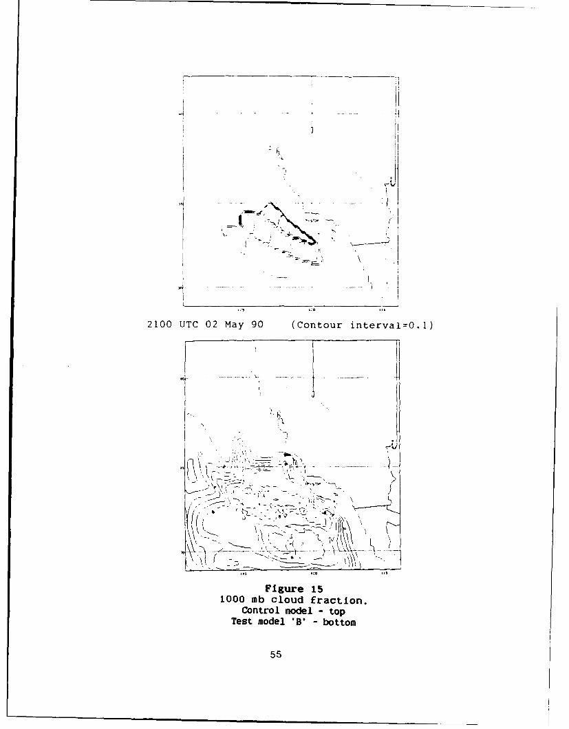
2. Cloud Fractions (Control Model vs Test Model 'B')-
Test model 'B', in addition to extending the low-
level cloud region westward similar to case 'A' , also
realistically extended the cloud region toward the
California coast (Figure 15). Since Stewart modified RH,
values to help produce more model-simulated clouds by using
satellite imagery and observations, this extension of clouds
along the coastline can be expected.
Satellite imagery (2030 UTC visible image, Figure 9)
showed a low-level tongue of coastal cloudiness from
Monterey Bay to San Luis Obispo Bay that the model did not
simulate. In addition. the model predicts low-level cloud
cover out about 100 nm seaward from the coast (34°N, 123' W)
where generally clear skies were observed. The sea surface
temperature (SST) fields used in these simulations were from
0000 UTC 02 May 1990 and kept constant throughout the time
period. The constant SST fields may be part of the reason
for the model cloud fraction weaknesses. SST values warmer
than or approximately equal to the surface air temperature
may result in more low-level clouds due to increased
boundary layer flux convergence while significantly cooler
model SST values could inhibit cloud formation.
As discussed in Section V, the control model's (and
subsequently the test model's) simulation of low-level winds
resulted in a much shorter duration southerly surge event as
54
115 .z1
iI
! i~
Fftu- 15__"Tes moe BIbto
2100 UTC 02 May 90 (Contour interva1=O.5)
,,.*.4. . . . . .
S. .. ." m '- • i -
\ - \ - _- ' 7 .•'i < -' I!• \ • !
. ,_.. .. _ • - _--.--_.-,.---•- . _.,, , ,.-
I, -~Figure 151000 mb cloud fraction.
Control model -topTest model "B' bottom
5S

comnpaed with wind :)bserviations along the _'ai.fornia coast.
Since the southerly surge often produces persistent coastal
cloudiness, the weaker model simulation of southerly winds
may be another cause of the model's weakness in producing
clouds up to the coastline.
The increased model-simulated cloud cover should
affect the radiation and temperature fields at and below the
cloud levels. This is evaluated in the following sections.
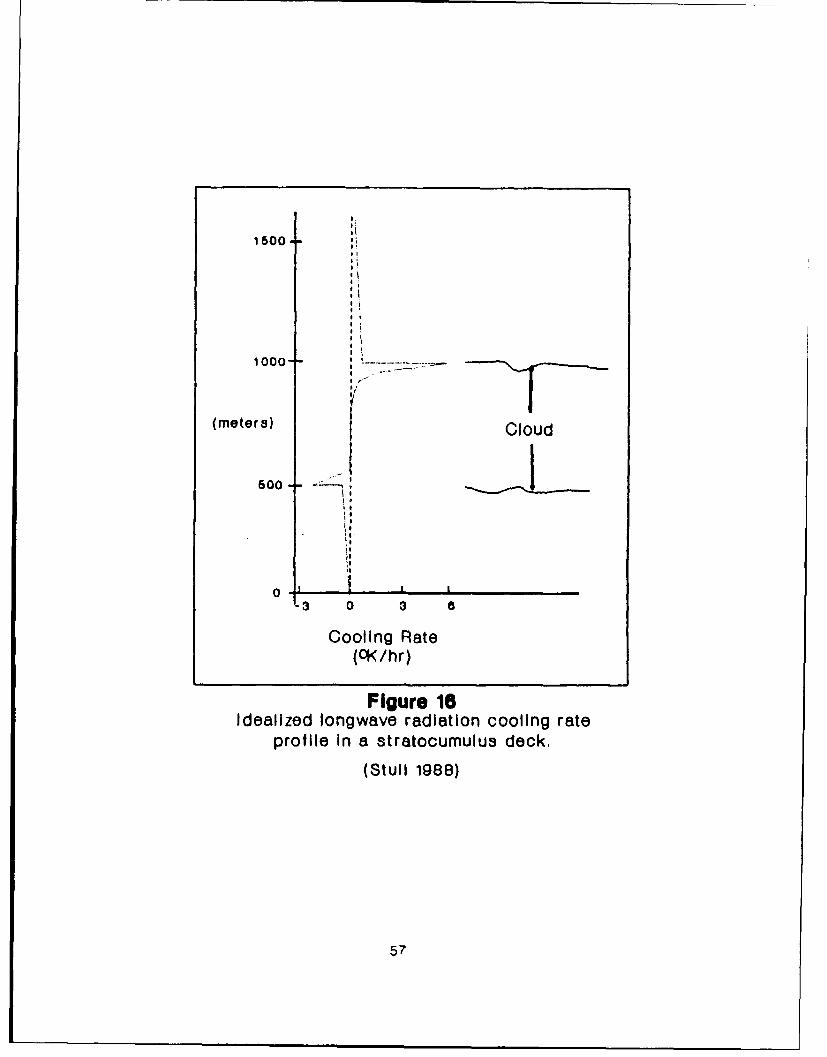
C. LONGWAVE RADIATION-
Figure 16 depicts an idealized longwave radiation
profile in relation to a stratocumulus cloud (Stull 1988).
A maximum longwave cooling rate is expected at the top of
the cloud boundary with minimal cooling above the cloud.
Also weaker longwave heating may be expected at the cloud
base.
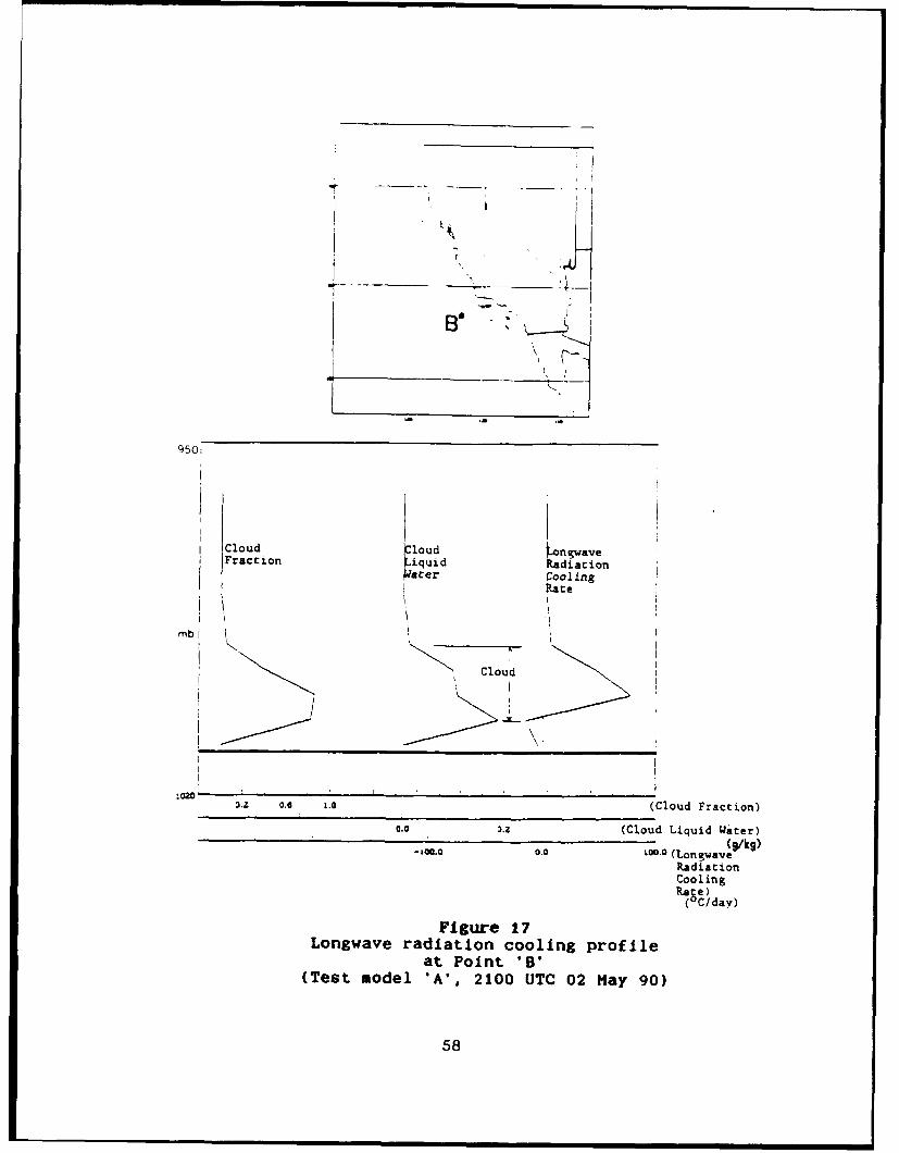
Longwave radiation along with cloud fraction and cloud
liquid water profiles are shown in Figure 17 for Point 'B'
(3T N,122 W) for test model 'A' at 2100 UTC 02 May. Cloud
tops occur at about 990 mb for both cloud fraction and cloud
liquid water representations. Also, cloud fraction and
cloud liquid water profiles depict the cloud base at about
1005 mb. Maximum longwave cooling of approximately 78°C/day
occurs within the cloud at about 1000 mb with a heating rate
of about 17 0 C/day at the cloud bottom. Evaluating this
56
1600.-',I
I.
1000
(meters) Cloud
6Y00 I:I ,I g
00
ait
3 0 3 8
Cooling Rate(OK/hr)
Figure 10Idealized Iongwave radiation cooling rate
profile in a stratocumulus deck,
(Stull 1988)
57
- a I
9501
Cloud Cloud ongwaveFraction .iquid Radiation
•Icer CoolingRate
mbI
-I-
o.0 1.0 (Cloud Fraction)
0.0 (Cloud Liquid Water)• ; (g / k 9)-0oa.0 0.0 00o0 (Lon gwave
RadiationCoolingPage)
( C/day)
FIgure 17Longwave radiation cooling profile
at Point 'B'(Test model 'A', 2100 UTC 02 May 90)
58

model radiation prorile with the ideai case represented
Figure 16 shows rhat the model's maximum longwave radiat
cooling is iepresented tavorably though the model ioca
the cooling maximum at a lower level within the clo
Incorporation of the cloud liquid water scheme provide
direct interaction of the cloud with the environmental
temperature and moisture profiles. This interaction is
evident in the equations (3.1. 3.6. and 3.7) as given by
Sundqvist. Thus changes in cloud liquid water as computed
at every gridpoint and tor each iteration in the model
directly impact the temperature and moisture of the
atmosphere.
However, these changes in cloud liquid water are not as
readily apparent when comparing cloud liquid water to cloud
fraction. This is because cloud fraction is computed along
with radiation parameters every half hour (60 iterations).
Thus the indirect effect of cloud liquid water on cloud
fraction through changes in temperature and moisture
profiles is not readily visible in comparisons. Hence,
cloud liquid water provides a more physically realistic
determination of cloud structure and subsequent radiation
profiles, though for comparisons of model simulations there
is a more direct, one-to-one relationship betwen cloud
fraction and radiation than cloud liquid water and
radiation.
59

D. TEMPERATURE-
Temperature tield comparisons revealed significant
dcfferences between the control model and test models 'A'
and 'B'. The temperature differences occurred within the
model-simulated cloud regions for both test models.
1. Temperature (Control Model vs Test Model 'A')-
Figure 18 shows low-level cross-section temperature
comparisons of the control model and test model 'A' for a
predominantly cloud-covered region from Point 'C' to 'D' at
2100 UTC 02 May. Temperatures were as much as 2°C lower
for test model 'A' versus the control model in areas within
and below the dense clouds. Figure 19 for Point 'B' shows
that temperature deviations occurred from the surface up to
about 960 mb with the maximum difference occurring within
the cloud boundaries.
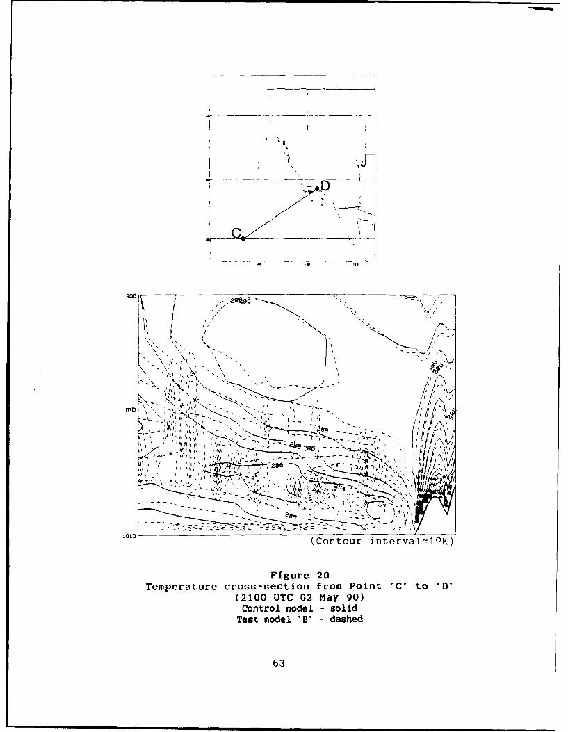
2. Temperature (Control Model vs Test Model 'B')-
Low-level cross-section temperature comparison for
the same region described above is shown in Figure 20.
Similar to test model 'A', temperatures in test model 'B'
were lower by as much as 4!C within cloud regions as
compared to the control model. The temperature field
60

iL
! I
"I / : 1
Z >.
1010
e, \.., '\ -
" " . . "6
" .,. - ' ".t .-•. \ ." ••• • • .- • • " - " •
I I L -4, •;-,' • , ,.,:. :- f,,,']. ,)
I.~ . . .' -" - - " • , "- - ,- - _• • - " - - /(Contou inter.l'NOK
Figur 18
1010

CloudiLiquidIWater
mb Temperaturt
Test 'A'
Control Clo ud
280.0 8. Q.9O0 .'"-TQ 1K)
Figure 19Temperature profile at Point 'B
(2100 IJTC 02 May 90)
62
900 -99
I.J,.
z~ -. I
~01C(Contour interval=lOK)
FIgure 20Temperature cross-section from Point 'C' to 'D'
(2100 UTC 02 May 90)Control model - solid
Test model 'B' - dashed
63

difference for this case appeared to be larger due to
thicker cloud depictions by the model.
Also comparable to test model 'A', Figure 21 for
Point 'B' shows temperature profile deviation occurring
within the same cloud boundary levels.
E. CLOUD LIQUID WATER-
Generally, low-level cloud liquid water regions closely
follow the cloud fraction regions as seen in Figure 22.
Note the rather smooth nature of cloud fraction (as
dependent on RH) in contrast to the somewhat noisy structure
of cloud liquid water.
An area of interest due to the lack of clouds at 1000 mb
is located in the region's southwest quadrant (Figure 23).
A comparison between the test model run 'B' 1000 mb cloud
fraction and cloud liquid water fields for 2100 UTC 02 May
show little or no cloud liquid water in that quadrant at
1000 mb. A cross section from point 'C' to 'D' (Figure 24)
shows cloud liquid water generally throughout that region
with relatively dry regions at the 1000 mb level. This
layered cloud structure is often observed in the marine
boundary layer. Use of the explicit cloud liquid water
scheme allows for a realistic depiction of this layered
structure that a simple cloud fraction scheme could not
simulate. Note how the cloud liquid water cross section
64

I. i
B°~
"CloudLiquid
Temperatu e Water
mb/ _
Test B' I
/ •Cloud
"Control
280.0 .8.0 -a. (T.K
Figure 21
Temperature profile at Point 'B'(2100 UTC 02 May 90)
65

Cloud Fractioncontour interval=O.1
v-
3 -
- ,
...........-
j,--- )
Cloud Liquid Water .. 00It" I
Ib
FIgure 221000 ab cloud fraction (top)
1000 mb cloud liquid water (b-tto,)(Test model 'A', 2100 UTC 02 May 90)
66

Cloud Fraction
- contour interval0O.
I/I
VL
Clu Liui WaterL
c A
1 : . ... . ..,............. I . .... ...... .. ..t
ClOud Liquid Water (bottom)contour intervaI=O.1 g/ .g .4k . . .
I'i I I)
Figure 231000 mb cloud fraction (top)
1000 nib cloud liquid water (bottom)
(Test model "B', 2100 UTC 02 May 90)
67

C O__
900
contour intervals:Cloud liquid water=O.1 g/kgCloud fraction=O.1
mb --
:.-- ---------
.- - ------- "-- -- -
1.010
Eloarzontal distance = 873.8 km
Figure 24Cloud liquid water (solid) and
cloud fraction (dashed) cross-sectionsfrom Point 'C' to 'D'.
(Test model 'B'. 2100 UTC 02 May 90)
68

a i -( pr ov 1i des a I-ore Ifa 1 i C hr I zOrIt a=I ac a er t (:-cal c 1 oud
texture appearance than the cloud traction contours as
compared in Figure 24. The cloud fraction is simply a
representation of RH while cloud liquid water includes more
of the physics needed in defining clouds and the boundary
layer.
69

VII. 'ONCLUSIONS AND RECOMMENDATIONS
A. CONCLUSIONS-
This study has demonstrated that the incorporation of
the Sundqvist et al. (1989) explicit non-convective cloud
liquid water scheme into the NRL mesoscale model provides
improvements in simulating longwave radiation, temperature,
and cloud structure features over the U.S. West Coast
Pacific region.
One limitation that was found in the incorporation of
the Sundqvist scheme for this particular case was its
extreme weakness in accurately diagnosing low-level clouds.
The main reason for this weakness was Sundqvist's
representation of relative humidity threshold values for
cloud formation. Test model evaluations were therefore
conducted using Sundqvist's cloud liquid water scheme but
retaining Slingo's critical relative humidity profile for
cloud formation (test model 'A'). In addition, test model
'B', which used a modified critical relative humidity
profile by Stewart (1992) was also evaluated. This modified
profile was proposed to help compensate for the control
model's weakness in diagnosing low-level clouds over certain
areas in the region. Test models 'A' and 'B' were able to
provide a closer cloud cover picture of the region as
70

compared to satellite imagery, with test model 'B' showing
more realistic cloud cover near the coast.
Longwave radiation profiles in cloud regions showed
realistic and consistent cooling and warming rates as
compared to idealized radiation profiles. Temperature
effects due to model-simulated cloud cover also compared
favorably.
A significant improvement in the NRL model was the
realistic horizontal and vertical cloud structure that was
represented by the cloud liquid water fields. Control model
cloud depiction was only through cloud fraction, a
representation of relative humidity. The introduction of
cloud liquid water as a prognostic variable takes into
account more of the physics involved in better defining
cloud structure and the marine boundary layer. Cloud liquid
water used as a portrayal of cloud cover provides a more
physically realistic texture and layered structure
associated with non-convective clouds.
71

B. RECOMMENDATIONS-
Stewart's (1992) study provided a modified RHc prorile
to help provide a closer cloud depiction as compared to
satellite imagery. Using this modified profile, better
cloud cover representation was achieved but continued fine-
tuning of the RH, values for a variety of cases of differing
synoptic flow may be necessary for a more accurate model
cloud cover picture. An experiment utilizing a good
dispersal of surrace, ship, and buoy station observations
with soundings along with satellite observations could
provide a closer real world RH, profile depiction.
Section VI described a situation where the 1000 mb cloud
liquid water depiction showed very little or no clouds while
satellite imagery clearly indicated low-level cloud cover
over the area. A cross-section view of the test model cloud
liquid water fields revealed a layered cloud structure with
a dry area at the 1000 mb level. Development of a three-
dimensional display capability would help provide an easier
way of visualizing a complex cloud structure from cloud
liquid water. Computation of cloud fraction at every
iteration to correspond to cloud liquid water fields would
aid in visual interpretation of clouds. In addition, other
fields in the model may be easier visualized three-
dimensionally.
72

This study incorporated rhe Sunaqvist &t al. 1989) non-
convective -loud scheme into the NRL model but did not
include Sundqvist>- scheme ror convective clouds. Further
study incorporating the convective cloud scheme is
recommended as a follow on.
Finally, an evaluation of the realistic cloud structure
by cloud liquid water in regions of available data could
verify the accuracy of the cloud portrayals and provide a
better degree of confidence in the overall model ,)utputs.
73
REFERENCES
Bosart, L.F.. 1983: 'Analysis of a California Eddy Event.'Mon. Wea. Rev., 111. 1619-1633.
Chang, S.W., 1979: "An Efficient Parameterization orConvective and Non-Convective Planetary Boundary Layersfor Use in Numerical Models, J. Appl. Meteor., 18,1205-1215.
Chen. C., and W.R. Cotton, 1987: "The Physics of the MarineStratocumulus-capped Mixed Layer." J. Atmos. Sci., 44.2951-2977.
Corkill, PW.. 1991: Synoptic and Mesoscale FactorsInfluencing Stratus and Fog in the Central CaliforniaCoastal Region, Master's Thesis, Meteorology Department,Naval Postgraduate School, Monterey, California.
Dorman, C.E., 1985: "Evidence of Kelvin Waves inCalifornia's Marine Layer and Related Eddy Generation."Mon. Wea. Rev., 113, 827-839.
Grandau. F.J., 1992: Evaluation of the Naval ResearchLaboratory Limited Area Dynamical Weather PredictionModel: Topographic and Coastal Influences Along the WestCoast of the United States, Master's Thesis, MeteorologyDepartment, Naval Postgraduate School, Monterey,California.
Harshvardhan. R. Davies, D.A. Randall, and T.G. Corsetti,1987: "A fast Radiation Parameterization forAtmospheric Circulation Models," J. Geophys. Res.. 92,1009-1016.
Holt, T., and S. Raman, 1988: "A Review and ComparativeEvaluation of Multi-level Boundary LayerParameterizations for First Order and Turbulent KineticEnergy Closure Schemes," Rev. Geophys.. 26, 761-780.
Kuo, H.L., 1974: "Further Studies of the Parameterizationof the Influence of Cumulus Convection on Large ScaleFlow," J. Atmos. Sci., 31, 1232-1240.
74
Mada I a. R. V. . .. W . 'hang, J. r.' . M rial tyY ; - Mactari, R K,Pallwal, V.B. Sarin. T. Holt, and S. Raman. 1987:Description ot the Naval Research Laboratory LimitedArea Dynamical Weather Prediction Model. NRL TechnicalReport 5992.
Mass, C.F., and M.D. Albright, 1989: "Origin (-t theCatalina Eddy, Mon. Wea. Rev., 117. 2406-2436.
Slingo, J.M., and B. Ritter, 1985: 'Cloud Prediction in theECMWF Model, ECMWF Tec. Rep. No. 46, 48 pp.
Stewart, P.C., 1992: Incorporation of a RadiationParameterization Scheme into the Naval ResearchLaboratory Limited Area Dynamical Weather PredictionModel, Master's Thesis. Meteorology Department, NavalPostgraduate School. Monterey, California.
Stull, R.B., L988: An Introduction to Boundary LayerMeteorology. Kluwer Academic Publishers.
Sundqvist, H., 1988: "Parameterization of Condensation andAssociated Clouds in Models for Weather Prediction andGeneral Circulation Simulation,' Physically-BasedModelling and Simulation of Climate and Climatic Change,M.E. Schlesinger, Ed.. Reidel, 433-461
Sundqvist, H., E. Berge, and J.E. Kristjansson. 1989:"Condensation and Cloud Parameterization Studies with aMesoscale Numerical Weather Prediction Model," Mon. Wea.Rev. 117, 1641-1657.
75
INITIAL DISTRIBUTION LIST
No. Copies
1. Defense Technical Information Center 2Cameron StationAlexandria, VA 22304-6145
2. Library, Code 52 2Naval Postgraduate SchoolMonterey, CA 93943-5002
3. Chairman (Code MR/Hy)Department of liteorologyNaval Postgraduate SchoolMonterey, CA 93943-5000
4. Chairman (Code OC/Co)Department of OceanographyNaval Postgraduate SchoolMonterey, CA 93943-5000
5. Professor Teddy R. Holt (Code MR/Ht) IDepartment of MeteorologyNaval Postgraduate SchoolMonterey, CA 93943-5000
6. Professor Philip A. Durkee (Code MR/De)Department of MeteorologyNaval Postgraduate SchoolMonterey, CA 93943-5000
7. Dr. Simon ChangNaval Research Laboratory Code 7220Washington, D.C. 20375
8. Dr. John Hovermale INaval Research Laboratory-MoncereyMonterey, CA 93943-5006
9. Dr. Lee EddingtonGeophysics DivisionPacific Missile Test CenterPoint Mugu, CA 93042-5000
76

10. Dr. Gary Geernaertoffice of Naval Research
Code 1122MM800 N. Quincy St.Arlington, VA 22217-5000
11. LCDR Damacene V. FerandezNaval Oceanography Command DetachmentPSC 486, Box 1243FPO, AP 96506-1243
77