Embed Size (px)
Citation preview
AD-A280 993
NAVAL POSTGRADUATE SCHOOLMONTEREY, CALIFORNIA
THESIS
ANALYSIS OF THE FIRST SUCCESSFUL FLIGHT OF
GPS ABOARD THE SPACE SHUTTLE
by
Stephen Paul Rehwald, Jr.and
Carolyn Louise Tyler
March 1994
Thesis Advisor Randy L. Wight
Approved for public release; distribution is unlimited.
DTIC QUALITYP T4,7ED 3
94-20401
7 5 112
UNCLASSIFIEDSECURITY CASIICATiON OF THIS PAGE
IlPORT DllMIUNTATION PAEPI a REPORT SECURITY CLASSIFICATION UNCLASSIFIED lb. RESTRICTIVE MARKINGS
2a SECURITY CLASSIFICATION AUTHORITY 3. D1bTNIBUTIOI/AVAILABIUTY OF REPORT
2b. DECLASSIFICATIONIDOWNGRADING SCHEDULE Approved for public release;distribution is unlimited
4. PERFORMING ORGANIZATION REPORT NUMBER(S) 5. MONITORING ORGANIZATION REPORT NUMBER(S)
6a. NAME OF PERFORMING ORGANIZATION 61. OFFICE SYMBOL 7a. NAME OF MONITORING ORGANIZATIONNd(i•appih,) Naval Postgraduate SchoolNaval Postgraduate School [ Code 31
6c. ADDRESS (City, State, and ZIP Code) 7b. ADDRESS (City, State, and ZIP Code)
Monterey, CA 93943-5000 Monterey, CA 93943-5000
Sa. NAME OF FUNDING/SPONSORING T8b. OFFICE SYMBOL 9. PROCUREMENT INSTRUMENT IDENTIFICATION NUMBERORGANIZATION j (if appicable)
8c. ADDRESS (City, State. and Z2P Code) 10. SOURCE OF FUNDING NUMBERSPROGRAM PROJECT TASK WORK UNITELEMENT NO. NO. NO. ACCESSION NO.
11. TITLE (Inekuid Security Cklaftatn)ANALYSIS OF THE FIRST SUCCESSFUL FLIGHT OF GPS ABOARD THE SPACE SHUTTLE
I2. PERSONAL AUTHOR(S)Rehwald, Stephen P., and Tyler, Carolyn L.13a. TYPE OF REPORT I11)'. TIME COVERED r14. DATE OF REPORT (Yeaw. Month Day) I15. PAGE COUNTMaster's Thesis I FROM 02/93 To 03/94 1 March 1994 I ill16. SUPPLEMENTARY NOTATIUN The views expressed in this thesis are those of the authors and do not reflect
the official policy or position of the Department of Defense or the United States Government.
17. COSATI CODES 18. SUBJECT TERMS (Contnue on reiven if necessay and identiy by block number)FIELD GROUP SUB-GROUP Global Positioning System, GPS, Space Shuttle, Kalman Filtering,I ICoordinte Transformation, State Vector.
19. ABSTRACT (Continue on reveae if nec...wy and identify by block number)
A Trimble Advanced Navigation Sensor (TANS) Quadrex Global Positioning System (GPS) receiver pro-cessing unit and three antenna/preamplifier assemblies were flown aboard Space Shuttle Discovery, STS-51, aspart of DTO 700-6, GPS On-orbit Demonstration (GOOD). The experiment was designed to quantify advantagesand identify potential problem areas for Space Shuttle GPS operations using a low cost, commercial, space config-ured, GPS receiver. GPS data, including position, velocity, time, health, and status information were recordedduring the mission. Following the mission, a reference trajectory was generated by NASA Johnson Space Centerthrough post-processing of the Orbiter's on board navigation state. The recorded GPS data has been analyzed andcompared to the reference trajectory to evaluate the navigational performance of the receiver. Additionally, post-flight filtering of the GPS data has been performed in order to determine whether a significant increase in perfor-mance may be obtained through filtering. 3
20. DISTRIBUTIONAVAILABIUTY OF ABSTRACT 21. ABSTRACT SECURITY CLASSIFICATION
[] UNCLASSIFRED/UNMMITED [] SAME AS RPT. Q] DTIC USERS UNCLASSIFIED22a. NAME OF RESPONSIBLE INDIVIDUAL 12. TELEPHONE (Include Area Code) 2c.OFFICE SYMBOLRandy L. Wight (408) 646-2491 SP/Wt
DO FORM 1473,84 MAR 83 APR edition may be used until exhausted SECURITY CLASSIFICATION OF THIS PAGEAll odw edons ae obsolet• UNCLASSIFIED
i
Approved for public release; distribution is unlimited
ANALYSIS OF THE FIRST SUCCESSFUL FLIGHT OF GPSABOARD THE SPACE SHUTTLE
byStephen Paul Rehwald, Jr.
Lieutenant, United States NavyB.S., United States Naval Academy, 1986
and
Carolyn Louise TylerLieutenant, United States Navy
B.S., Mary Washington College, 1986
Submitted in partial fulfillment of the
requirements for the degree of
MASTER OF SCIENCE IN ASTRONAUTICAL ENGINEERING
from the
NAVAL POSTGRADUATE SCHOOLMarch 1994
Authors: __ _ _ _ __ _ _ _ _ __ _ _ _ _
-Sehn Paul Rehwald, Jr. '"
Approved By:SqDR RajL ih^ei dvisor
Dr. 1 os Second Reader
,*nt r D. 1:Clla Ca.ý 'Dep Ot of Aeronautical and Astroha ugineering
ii
ABSTRACT
A Trimble Advanced Navigation Sensor (TANS) Quadrex Global Positioning Sys-
tem (GPS) receiver processing unit and three antenna/preamplifier assemblies were
flown aboard Space Shuttle Discovery, STS-5 1, as part of DTO 700-6, GPS On-orbit
Demonstration (GOOD). The experiment was designed to quantify advantages and iden-
tify potential problem areas for Space Shuttle GPS operations using a low cost, commer-
cial, space configured, GPS receiver. GPS data, including position, velocity, time,
health, and status information were recorded during the mission. Following the mission,
a reference trajectory was generated by NASA Johnson Space Center through post-pro-
cessing of the Orbiter's on board navigation state. The recorded GPS data has been ana-
lyzed and compared to the reference trajectory to evaluate the navigational performance
of the receiver. Additionally, post-flight filtering of the GPS data has been performed in
order to determine whether a significant increase in performance may be obtained
through filtering.
Acessulon For
NTIS GR!A&IDTIC TAB ElUwiri•armolced 0J*5tilfcatic
ByDistributi n 4c • .
Availability OedesAvail and/or
Dist Special
iil "' 1
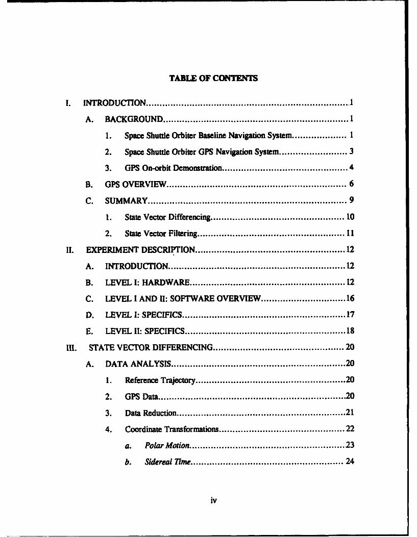
TABLE OF CONTENTS
INTRODUCTION ........................................................................... 1
A. BACKGROUND .................................................................... 1
1. Space Shuttle Orbiter Baseline Navigation System ................. 1
2. Space Shuttle Orbiter GPS Navigation System ...................... 3
3. GPS On-orbit Demomtration .......................................... 4
B. GPS OVERVIEW ............................................................... 6
C. SUMMARY ...................................................................... 9
1. State Vector Differencing .............. . .................................. 10
2. State Vector Filtering .................................................. 11
II. EXPERIMENT DESCRIPTION .................................................... 12
A. INTRODUCTION ............................................................. 12
B. LEVEL I: HARDWARE ......................................................... 12
C. LEVEL I AND II: SOFTWARE OVERVIEW ............................ 16
D. LEVEL I: SPECIFICS .................. .......................... 17
E. LEVEL 11: SPECIFICS ....................................................... 18
III. STATE VECTOR DIFFERENCING ............................................ 20
A. DATA ANALYSIS ............................................................. 20
1. Reference Trajectory .................................................... 20
2. GPS Data ................................................................. 20
3. Data Reduction ........................................................ 21
4. Coordinate Transformations .......................................... 22
a. Polar Motion ...................................................... 23
b. Sidereal lime .................................................... 24
iv
c. Astronomic Nwahion .................................................. 25
d. General Precession ..................................................... 27
e. Standard Epoch Conversion ........................................ 27
5. Summary .................................................................... 27
B. NAVIGATION PERFORMANCE .............. ....................... 28
IV. STATE VECTOR FILTERING ......................................................... 37
A. INTRODUCTION ................................................................. 37
1. The Purpose for a Filter .................................................. 37
B. KALMAN FILTER ............................................................... 38
1. Theoretical Model ......................................................... 38
2. Theoretical Equations ................ . . ............. 39
C. AN ADAPTATION OF THE KALMAN FILTER ......................... 41
1. Analysis of Problem .......................................................... 41
2. Diagram of the Kalman Filter .............................................. 42
3. Description of the Kalman Filter Design ............................... 43
D. RESULTS FROM USING A KALMAN FILTER .......................... 44
E. SUMMARY ........................................................................ 52
V. ERROR SOURCES ...................................................................... 53
A. PREDOMINANT ERROR SOURCES ....................................... 53
B. ERRORS SPECIFIC TO EXPERIMENT ..................................... 56
C. POST FLIGHT ANALYSIS .................................................... 60
VI. CONCLUSIONS ........................................................................ 62
A. FLIGHT HARDWARE ......................................................... 62
B. FLIGHT SOFTWARE ........................................................... 63
C. FUTURE APPLICATIONS ........................................................ 63
APPENDIX A (WGS 84 TO MS0 COMPUTER PROGRAM) .......................... 64
V
APPENDIX B (RSS DIFFERENCING COMPUTER PROGRAM) .................... g2
APPENDIX C (TANSGRAPH PLOTS) ....................................................... 85
APPENDIX D (KALMAN FILTER COMPUTER PROGRAM) ......................... 92
LIST OF REFERENCES ...................................................................... 97
BIBLIOGRAPHY ............................... . ...................................... ... 98
INITIAL DISTRIBUTION LIST ................................................................ 99
vi
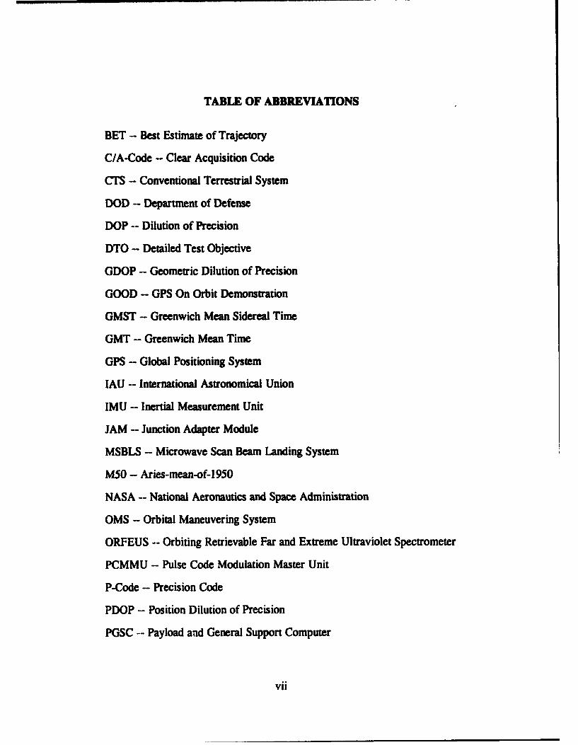
TABLE OF ABBREVIATIONS
BET - Best Estimate of Trajectory
C/A-Code - Clear Acquisition Code
CTS - Conventional Terrestrial System
DOD - Department of Defense
DOP -- Dilution of Precision
DTO - Detailed Test Objective
GDOP -- Geometric Dilution of Precision
GOOD - GPS On Orbit Demonstration
GMST - Greenwich Mean Sidereal Time
GMT -- Greenwich Mean Time
GPS - Global Positioning System
IAU - International Astronomical Union
IMU - Inertial Measurement Unit
JAM - Junction Adapter Module
MSBLS - Microwave Scan Beam Landing System
MS0 - Aries-mean-of-1950
NASA -- National Aeronautics and Space Administration
OMS - Orbital Maneuvering System
ORFEUS -- Orbiting Retrievable Far and Extreme Ultraviolet Spectrometer
PCMMU -- Pulse Code Modulation Master Unit
P-Code - Precision Code
PDOP - Position Dilution of Precision
PGSC -- Payload and General Support Computer
vii
PPS - Precise Positioning Service
RCS - Reaction Control System
RF -- Radio Frequency
SA-- Selective Availability
SPAS - Shuttle Palette Satellite
SPS - Standard Positioning Service
STS - Space Transportation System
TACAN - Tactical Air Navigation
TANS - Trimble Advanced Navigation Sensor
TDOP - Time Dilution of Precision
TDRS - Tracking and Data Relay Satellite
UTC - Coordinated Universal Time
UTI - Universal Time I
WGS84 - World Geodetic System 1984
viii
ACKNOWLEDGEMENT
The authors would like to express their heartfelt gratitude to the crew of STS-51
(Frank Culbertson, Bill Readdy, Jim Newman, Carl Walz, and Dan Bursch) for making
this thesis possible. Our sincere appreciation goes also to Penny Saunders for sharing her
valuable time and vast GPS expertise with us. Thanks to Flora Lowes for providing the
STS-51 reference trajectory, and to Ed Brown whose assistance with coordinate trans-
formations was invaluable. Thanks also to Tom Silva whose support went far above the
call of duty. Locally, we would like to thank CDR Randy Wight, our thesis advisor, for
his support and encouragement throughout the past year. Special thanks go to Dr. Titus
and LTjg Dimitris Kataras, Hellenic Navy, for their assistance with the filter design.
Finally, we would like to thank God for guiding us through this entire experience.
ix
I. INTRODUCTION
This thesis investigated the performance of a low cost, commercial, space config-
ured, Global Positioning System (GPS) receiver' flown aboard Space Shuttle Discovery,
STS-51, as part of DTO 0700-6,2 GPS On-orbit Demonstration (GOOD). The DTO was
sponsored and funded by NASA Johnson Space Center, and developed with the support
of NASA contractors, and students, including the authors, from the Naval Postgraduate
School. Data recorded during the mission was analyzed to evaluate navigational perfor-
mance of the receiver. Additionally, post-flight filtering of this data was performed in
order to determine whether a significant increase in performance could be obtained
through filtering.
A. BACKGROUND
1. Space Shuttle Orbiter Baseline Navigation System
A wide variety of equipment is employed in the Orbiter's baseline navigation
system. All navigation sensor information is supplied to a six-state suboptimal Kalman
filter, which provides the navigation functions with three position and three velocity
states. The three position states are the coordinates specifying the Orbiter's position vec-
tor in the Aries-mean-of-1950 (M50) Cartesian coordinate system. 3 Likewise, the three
velocity states define the Orbiter's velocity vector in the M50 system.
1Trimble Advanced Navigation Sensor (TANS) Quadrex GPS Receiver Processor Unit.
2 Detailed Test Objective Number 0700-6.
3 The MS0 system is defined in NASA Technical Memorandum X-58153, October 1974.
During the ascent phase of a mission, the Inertial Measurement Unit (IMU)
is the primary sensor, providing attitude and acceleration data to the Kalman filter. This
data is augmented by ground based C-band radar-tracking information uplinked over an
S-band communication link. During the on-orbit coasting phase of a mission, the IMU
provides attitude data, and acceleration data from Orbital Maneuvering System (OMS)
burns. Accelerations falling below the IMU threshold arise from opposing Reaction
Control System (RCS) thrusters that do not form a perfect couple (vernier effect), and
from external venting of gasses and waste products. These unaccounted for accelerations
result in steadily increasing navigational error.
While on-orbit, the ground continues to track the Orbiter using ground-based
C-band radar. Two-way Doppler tone ranging over S-band and Ku-band communication
links, either direct or via the Tracking and Data Relay Satellite (TDRF) system, provides
additional tracking capability. When the Orbiter's navigational state is observed to devi-
ate from the ground based tracking trajectory by a pre-defined, mission-dependent
amount, a new state vector consisting of three position states, three velocity states, and a
time tag is uplinked by Mission Control. At various times during a mission (prior to ren-
dezvous and deorbit burn), an IMU alignment may be performed using an on board star-
tracker to correct attitude error caused by gyro drift.
During the re-entry phase of a mission, IMU data is augmented with drag
modeling data from 250,000 feet down. As the Orbiter passes through the ionosphere,
all radio-navigation and communication signals are blacked out for a period of time.
Upon exit from blackout, contact is first established by C-band tracking radar. A state
vector can be uplinked as soon as S-band communication is regained. Subsequently, the
Orbiter can receive L-band Tactical Air Navigation (TACAN) station signals and begin
area navigation, combining TACAN range and bearing data with barometric (30,000-
2,500 feet) aid radar (2,500 feet down) altimeter measurements. Final approach and
2
landing are accomplished with a microwave scan beam landing system (MSBLS), begin-
ning normally at 10,000 feet, 10 nautical miles downrange from touchdown.
2. Space Shuttle Orbiter GPS Navigation System
Pursuant to a study contract commissioned by NASA, Rockwell Internation-
al's Space Systems group conducted a design and integration study of a GPS-based pri-
mary navigation system for the Orbiter in the late 1970's. (Van Leeuwen et al, 1979, pp.
118-135) The study demonstrated that the use of on board satellite GPS receivers for
precise orbit determination was clearly feasible, and expected the improved navigation
.apabilities to yield significant operational benefits. The study concluded the GPS-based
system to be a technically sound and cost-effective proposition. Based on the study,
plans were laid to install a GPS navigation system in all Shuttle orbiters beginning in the
early 1980's, with follow-on goals of deleting certain equipment from the baseline navi-
gation system. Within about two years, however, the decision to install GPS was
reversed in favor of continuing with the baseline navigation configuration. Certain GPS
provisions, notably antennas, cabling, and bulkhead feedthroughs, were nevertheless
retained, and currently exist on all Orbiter vehicles. (Saunders, 1994, pp. 1-13)
The issue of GPS installation in the Orbiter fleet surfaced again in the early
1990's. Renewed interest was motivated by the planned phase out of TACAN stations.
Since TACAN was used as the Orbiter's primary navigation aid following exit from
blackout, through MSBLS acquisition, NASA considered suitable alternatives. Looking
at the direction the Department of Defense (DOD) and the Federal Aviation Administra-
tion were heading in, GPS was chosen as the replacement for TACAN. A developmental
test for the Orbiter GPS navigation system flew aboard STS-61 in December 1993, and
the system is presently expected to be operational in 1996. (Kachmar et. al., 1993, pp.
313-326)
3
3. GPS On-orbit Demeofrmtion
In mid-1992, with the foundation for installing an Orbiter GPS navigation
system laid, the crew of STS-51 conceived the GOOD DTO as a low cost pathfinder
project, to look at GPS in orbit, to quantify advantages, and identify potential problem
areas for Space Shuttle operations. Data from the DTO could then be used to comple-
ment the more highly integrated GPS Development Flight Test. Since STS-51 would
carry another payload with its own GPS receiver, the Orbiting Retrievable Far and
Extreme Ultraviolet Spectrometer-Shuttle Palette Satellite (ORFEUS-SPAS), the DTO
would also permit the evaluation of relative GPSI. Successful utilization of GPS on the
Orbiter could show benefits for use on other programs, such as Space Station, or for use
as a utility with other primary and secondary payloads, which require precise location
and timing information. Initially, goals of this experiment were as follows:
* Evaluate receiver performance in orbit by comparing its state vector to that deter-mined by ground tracking and Orbiter IMU's.* Evaluate the number and location of GPS antennas required to provide best naviga-tion solutions for flight deck experiment applications.e Determine the quality of GPS data received during on-orbit operations by collectingGPS health data.* Evaluate the accuracy of relative GPS, using GPS receivers both in the crew cabinand on ORFEUS-SPAS, with Orbiter radar and laser rangefinders as a reference.* Evaluate postflight the accuracy of relative GPS using data from Orbiter and SPASGPS receivers.
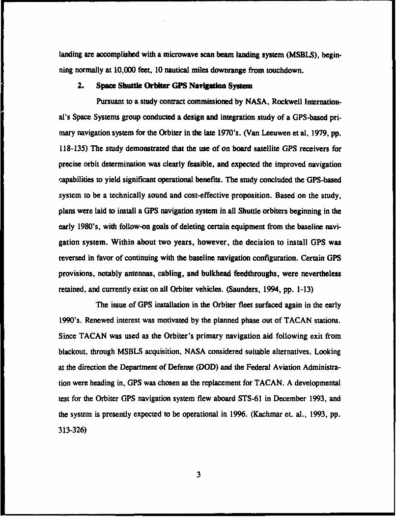
One of the computer displays developed for this DTO showed the magnitude
of the position difference between the Orbiter GPS and Orbiter IMU based state vectors
versus time.
1 Aspects of relative GPS are covered in the thesis "Theoretical Basis for State Vector Compari-
son, Relative Position Display, and Relative Position/Rendezvous Prediction" by LT Lester Makepeace,and the thesis "NPS State Vector Analysis and Relative Motion Plotting Software for STS-51" by LT LeeBarker.
4
Since error in the IMU based state vector increased with time, the root sum
square (RSS) difference (delta) between the GPS state vector and IMU state vector was
expected to increase with time. This difference was expected to collapse to zero when
Mission Control uplinked a new state vector based on ground tracking. This behavior
was first observed in orbit on flight day three, when a 20,000 ft. delta collapsed to about
300 feet following an update. An illustration of a similar event on the computer display
is shown in Figure I (the x-axis represents time, the y-axis represents RSS difference).
The close correlation between expected behavior and actual behavior indicated the GPS
position solution to be near truth.
6PSIN Position Oifferwme vs. Tim
Ortb-GP. 1S2O'O3803C.0OOrb-INS 19240:30Ib30.CLO
/ J ,
1 0M 0 4Ob.O 000tim.(uc mamqr) 1.464 Kit
tim E2WU sec
SAM F9 Ilt-FI Alt-F5 Alt-F I Alt-F7 IMt--S I Alt-FiI F10Alt ?1Ment To"*e ýreue Ser P~ut pFen 14pe one IMpe Plotsfbar one• S.tin
Figure 1: State Vector Differences vs. Time
5
B. GPS OVERVIEW
The GPS constellation consists of 21 operational satellites, and three active spares,
distributed in six orbital planes with three or four operational satellites in each plane.
The ascending nodes of each plane are separated by 600 intervals, and each plane has an
inclination relative to the equator of 55°. The satellites orbit at an altitude of 20,200 kin,
with a corresponding period of 12 hours. In comparison, the Space Shuttle orbits at an
altitude of approximately 300 km, with a corresponding period of 1' hours. The satel-
lites are positioned so that a minimum of five will normally be observable to a user
located anywhere on earth.
The satellites transmit on two frequencies: Li = 1575.42 MHz and L2 = 1227.6
MHz. The satellites transmit their signals using spread spectn" a techniques employing
two different spreading functions: a 1.023 MHz coarse/acquisition (C/A) code on Li
only and a 10.23 MHz precision (P) code on both Li and L2. Both P-code and C/A-code
enable a receiver to determine the range between the satellite and the user. Superim-
posed on both the P-code and the C/A-code is the NAVIGATION message (NAV-msg),
containing satellite ephemeris data, atmospheric propagation correction data, and satel-
lite clock-bias information. The TANS Quadrex GPS receiver flown on STS-51 utilizes
only the C/A-code on the Li frequency carrier.
Two levels of navigation are provided by the GPS; these are Precise Positioning
Service (PPS) and Standard Positioning Service (SPS). The PPS is a highly accurate
positioning, velocity, and timing service which is made available only to authorized
users through cryptographic keys. The SPS is a less accurate positioning and timing ser-
vice which is available to all GPS users. The TANS Quadrex GPS receiver flown on
STS-51 is an SPS receiver. In the future, receivers to be installed as part of the Orbiter
GPS navigation system will be PPS units. (Kachmar, et.al., 1993, pp. 313-326)
6
The SPS is specified to provide a 100 meter (95 % confidence) horizontal accuracy
to any GPS user during peacetime. This is approximately equal to 156 meters three-
dimensional (3-D) (95 % confidence) accuracy. SPS receivers can achieve approximately
337 nanosecond (95% confidence) Coordinated Universal Time (UTC) time transfer
accuracy. The SPS is primarily intended for civilian purposes, although it has many
peacetime military uses as well. The SPS horizontal accuracy specification includf
peacetime degradation of Selective Availability (SA) which is the dominant SPS L
source. I The SA position error distribution resembles a Gaussian distribution with a
long-term mean of zero. The SPS peacetime velocity degradation due to SA is classified.
The ranging codes broadcast by the satellites enable a GPS receiver to measure the
transit time of the signals and thereby determine the range between a satellite and the
user. The NAV-msg enables a receiver to calculate the position of each satellite at the
time of transmission of the signal. Four satellites are normally required to be simulta-
neously "in view" of the receiver for 3-D positioning purposes. This allows the user 3-D
position coordinates and the user clock offset to be calculated from the satellite range
and position data. Treating the user clock offset as an unknown eliminates the require-
ment for users to be equipped with precision clocks. Less than four satellites can be used
if the user altitude or system time is precisely known.
When the receiver has acquired the satellite signals from four GPS satellites,
achieved carrier and code tracking, and has read the NAV-msg, the GPS receiver is
ready to start navigating. The GPS receiver normally updates its pseudoranges and rela-
tive velocities once every second. The measurements are termed pseudorange because
ISPS did not routinely meet accuracy specs while the GPS system was undergoing test and verifi-cation by the DOD, prior to December, 1993. SA effects were often varied to further degrade accuracy.
7

the clock offset of a GPS receiver introduces a bias to the true range of the satellite. The
GPS receiver must know the GPS system time very accurately, because the satellite sig-
nals contain the time of transmission from the satellite in GPS time. The difference in
time between the signal leaving the satellite and arriving at the GPS receiver antenna is
directly proportional to the range between the satellite and the GPS receiver, so it is of
the utmost importance that the same time reference is used by both the GPS satellites and
the GPS receiver.
The GPS satellites carry two rubidium, and two cesium atomic frequency stan-
dards. However, the GPS receiver is not required to have a high accuracy clock such as
an atomic time standard. Instead, a crystal oscillator is used and the GPS receiver cor-
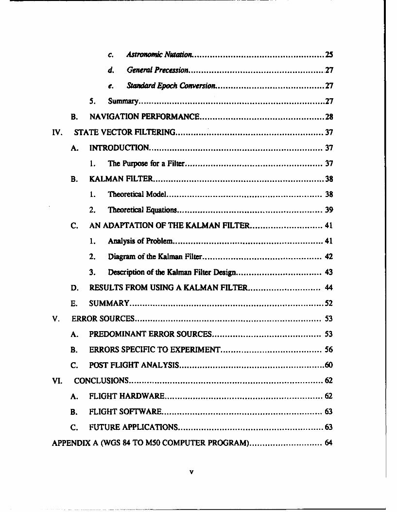
rects its offset from GPS system time by making four pseudorange measurements. The
GPS receiver can use the four pseudoranges to solve four simultaneous equations with
four unknowns. The position equations are shown in Figure 2. When the four equations
are solved, the GPS receiver has estimates of its position and GPS system time. The
GPS receiver velocity is calculated using the same types of equations, using relative
velocities instead of pseudoranges. GPS receivers perform most calculations using an
earth-centered earth-fixed coordinate system. They then convert to an earth model
defined by the World Geodetic System 1984 (WGS 84). WGS 84 is a very precise model
that provides a common grid system for transformations into other coordinate systems or
map datums.
Satellite coverage, as measured at the user antenna, can be affected by physical
obstructions, vehicle maneuvering or aspect, and basic receiver design. It therefore can-
not be categorized as a GPS system requirement or specification. Coverage is defined by
the orbits of the active satellites. The orbits determine the geometric relationships
between the satellites and the user, which the user measures as Position Dilution of Pre-
cision (PDOP). Since the geometric relationships continuously change as the satellites
8
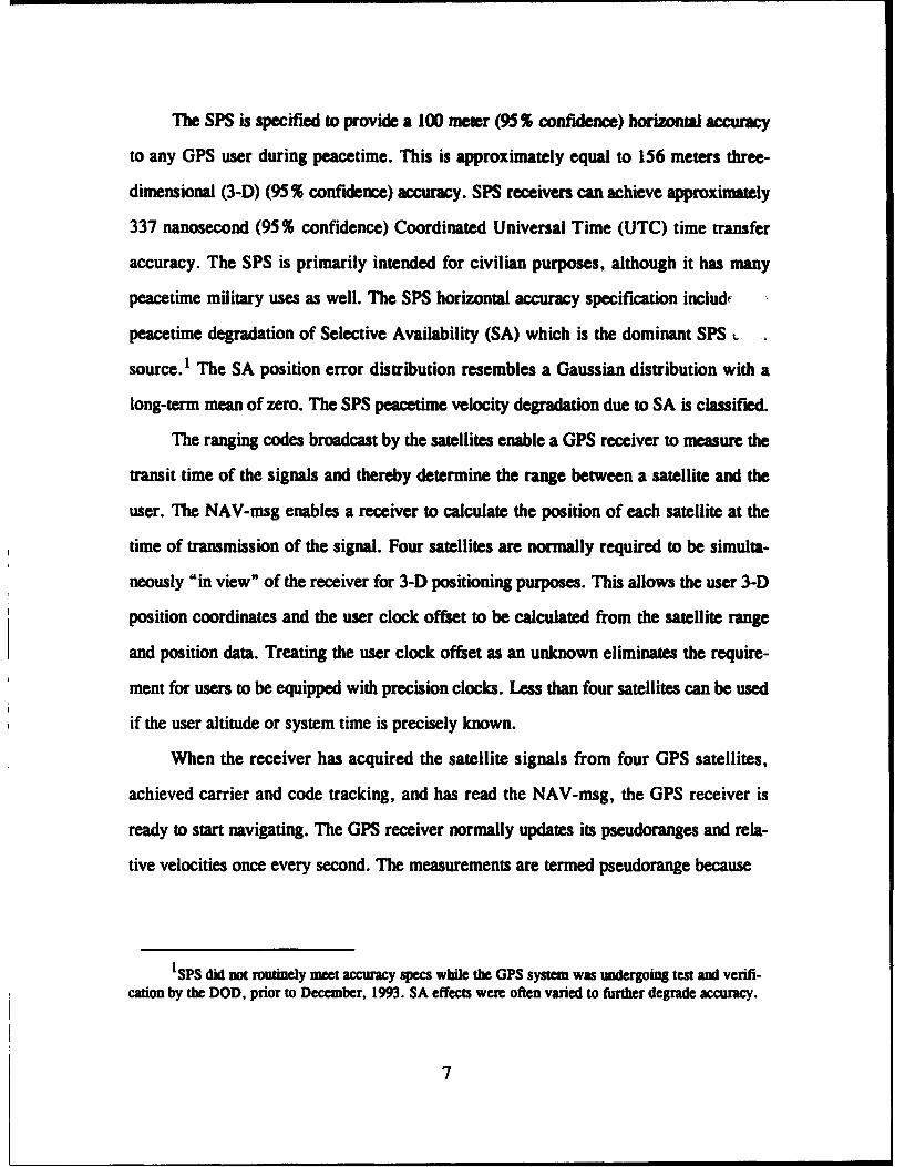
R, = cArl ( t-U 2+(Y y) l-U 2= ( RI C o)
R2 =cC 2 (x- U) 2 +(Y2 -U) 2 + ( z2 - UZ )2 = (R2 -G )2
R3 =cAt3 Y )2 + (Z3 _ UZ)2 = (R3 Co)2R4 =c 4 (x 4 - Ux) 2 + (y4 Uy) 2 +(z 4 - UZ) 2 =( R4 - )2
Ri = pseudorange
c = speed of light
Ati = time difference between signal leaving the satellite and arriving at the receiver
xi, yi, Zi = satellite position
Uy, Uy, Uz = receiver antenna position
C6 = receiver clock bias
Figure 2: GPS Position Equations
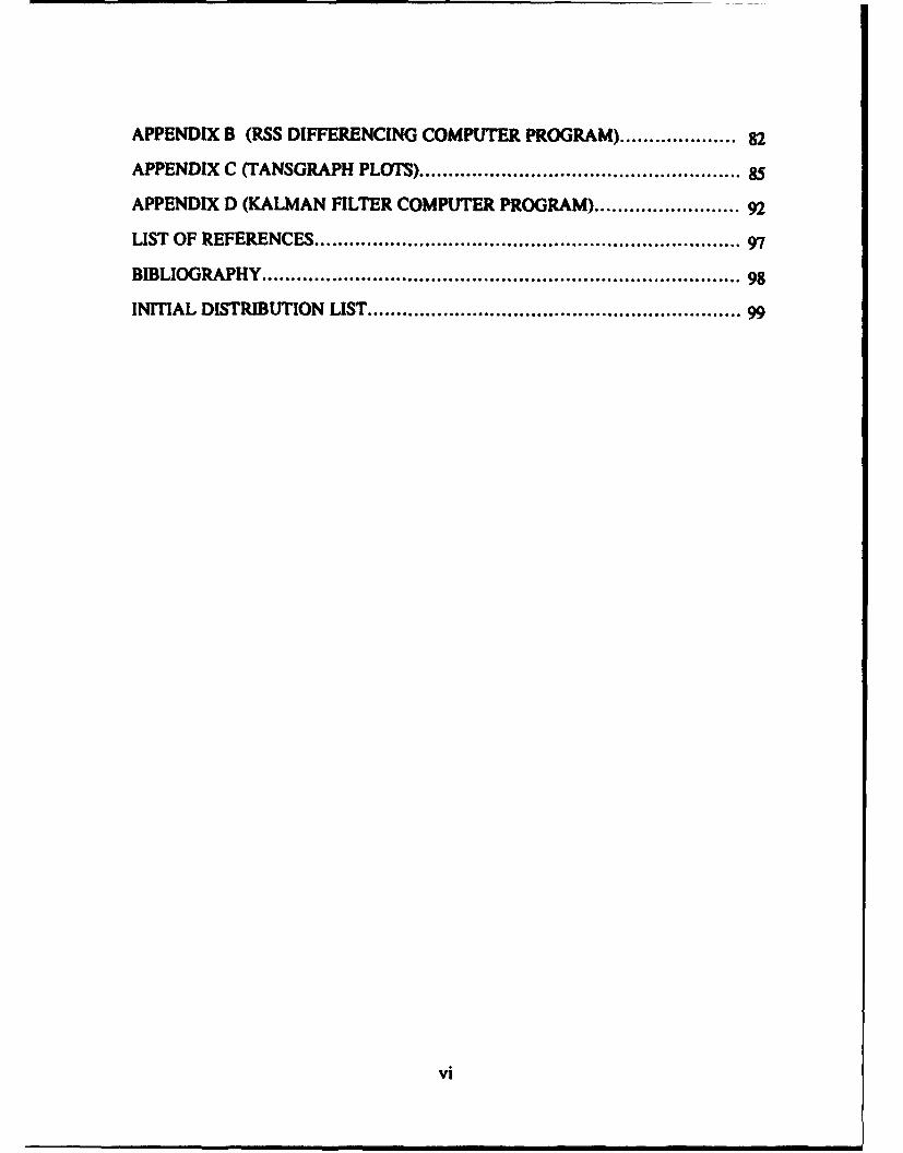
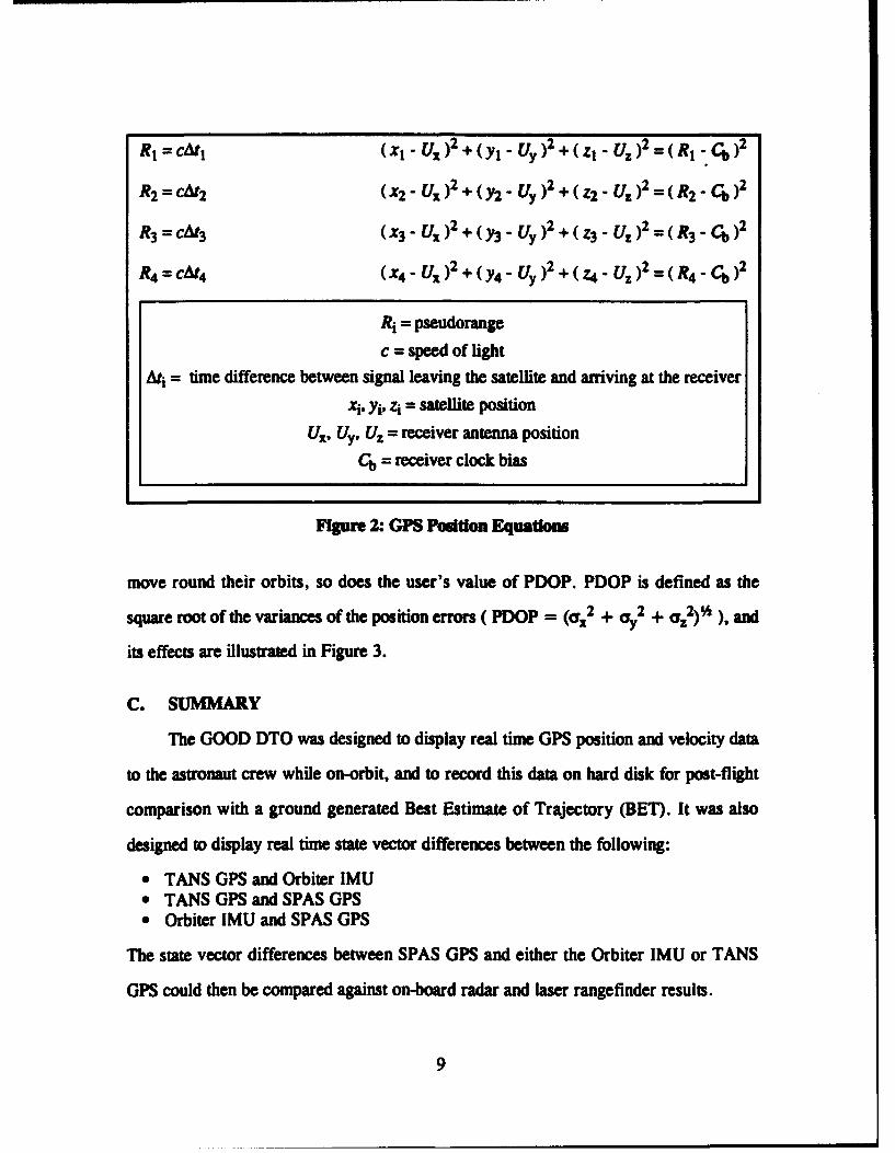
move round their orbits, so does the user's value of PDOP. PDOP is defined as the
square root of the variances of the position errors ( PDOP = (ox+2 + + CZ2) ), and
its effects are illustrated in Figure 3.
C. SUMMARY
The GOOD DTO was designed to display real time GPS position and velocity data
to the astronaut crew while on-orbit, and to record this data on hard disk for post-flight
comparison with a ground generated Best Estimate of Trajectory (BET). It was also
designed to display real time state vector differences between the following:
"* TANS GPS and Orbiter IMU"* TANS GPS and SPAS GPS"* Orbiter IMU and SPAS GPS
The state vector differences between SPAS GPS and either the Orbiter IMU or TANS
GPS could then be compared against on-board radar and laser rangefinder results.
9
/ R2
UNCERTAINTY
Figure 3: Effects of PDOP
1. State Vector Differenin*
Three prerequisites had to be satisfied before two state vectors could be com-
pared or differenced. These were as follows:
* Position and velocity elements were in the same frame of reference.* Time elements were in the same time scale.* Time elements were exactly matched.
Since the Shuttle navigation system used the MS0 Earth-centered Inertial
frame of reference, and the GPS receivers utilized the WGS 84 Earth-centered Earth-
fixed frame of reference, GPS state vectors were rotated from the WGS 84 reference
frame to the M50 reference frame prior to comparison with the Orbiter IMU state vec-
tor. This coordinate transformation will be addressed at length in a later chapter.
Since the Shuttle navigation system used Greenwich Mean Time (GMT), and
dhe GPS system used GPS time, GPS state vector times were adjusted to GMT prior to
10
comparison with Orbiter IMU state vectors. The Orbiter's clock was set according to the
National Bureau of Standards UTC standard, making the GMT time scale equivalent to
the UTC time scale in this application. The difference between UTC and GPS time was
transmitted in the NAV-msg by GPS satellites, and this value was used for the adjust-
ment.
Since the state vectors being compared were produced by independent sys-
tems, in general, the time elements did not match. The GOOD DTO utilized Cowell's
method to "propagate" the earlier state vector forward in time until its time element
matched the time element of the state vector it was being compared to. Although the dif-
ference between time elements was typically less than a second, it was significant at
orbital velocities of several kilometers per second. Quick and accurate propagation of
states is an active area of research, but will not be addressed further in these pages. 1
2. State Vector FUtering
Both the Ortiter IMU, and the SPAS GPS state vector outputs were filtered
in order to smooth the outputs over time, and to improve accuracy. The TANS GPS stat-
evector outputs, however, did not undergo filtering. Though use of a Kalman filter to
smooth the output would likely improve the TANS accuracy, a filter was not imple-
mented for the GOOD DTO due to time constraints. A Kalman filter has since been
designed for use with the TANS and will be addressed in 2i I-ter chapter.
1See the master's thesis of LT Lester Makepeace for a discussion of propagation, and an alternative
to Cowell's method for this application.
11
IL. E ER ENT DESCRIPTION
A. INTRODUCTION
The test objectives for this experiment were to demonstrate GPS on-orbit perfor-
mance at a relatively low cost. To meet this objective, NASA needed to:
* minimize interfaces to the Orbiter;* use "off-the-shelf" GPS technology;* designate this flight test as a non-critical (Detailed Test Objective) DTO; and,* limit hardware/software certification and qualification to ensuring crew safety.
Other objectives for this flight included collecting on-orbit GPS data to be pro-
cessed post flight, demonstrating the GPS performance to STS-51 crew real time, and
evaluating potential future use for this hardware and software.
The GOOD (GPS On-Orbit Demonstration) software was developed for use on a
GRID 386 laptop computer operating at 10 MHz. The desire was to provide the crew
with the capability to command and control the GPS receiver, and to display and record
GPS data for real time and postflight analysis. In February 1993, when our Naval Post-
graduate School team (LT Lee Barker, LT Les Makepeace, LT Steve Rehwald, and LT
Carolyn Tyler) arrived at NASA, Johnson Space Center, the flight hardware had already
been selected. The software used to interface with the TANS GPS receiver was being
fime-tuned to NASA's needs. Software used to provide real time analysis of the GPS data
had not been completed.
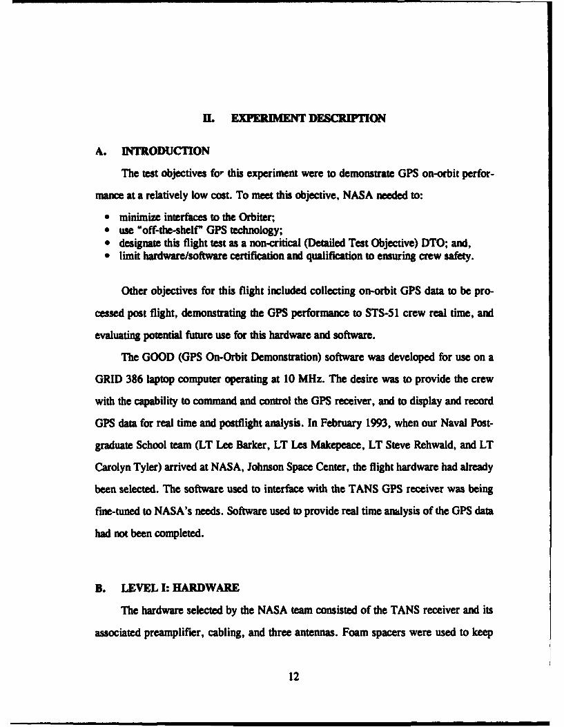
B. LEVEL I: HARDWARE
The hardware selected by the NASA team consisted of the TANS receiver and its
associated preamplifier, cabling, and three antennas. Foam spacers were used to keep
12
the antennas away from damaging the sensitive ultraviolet radiation protective coating on
the Orbiter's windows. Radio Frequency (RF) absorbers were placed behind the anten-
nas to minimize the RF disturbances in the crew cabin. Finally, the entire assembly was
attached to the window using velcro straps. As a safety requirement, a JAM (Junction
Adapter Module) was designed and built. The JAM was the only electrical interface to
the Orbiter and was required to protect the Orbiter from any adverse electrical behavior
generated by the GPS experiment. The hardware set up used aboard Discovery is shown
in Figure 4.
FIgure 4: Hardware Setup
13
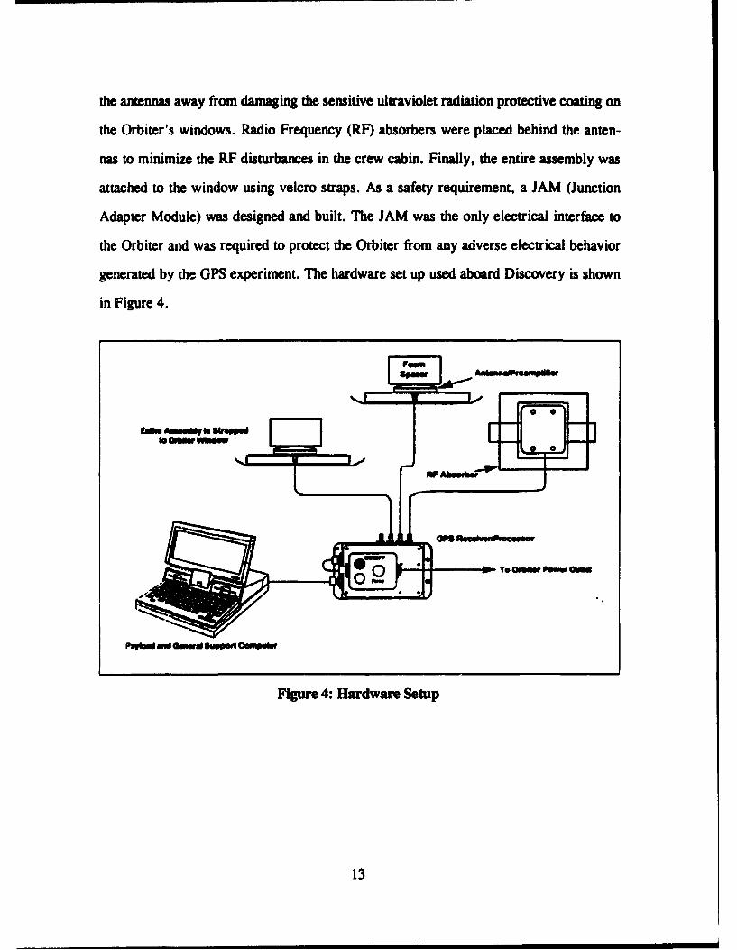
A more specific description of the TANS receiver used in this experiment is listed
in Table 1.
"iable 1: TANS RECEIVER DESCRIPTION
TANS Description Specification
Code / Carrier Tracked C/A code, Li
Channels 6
Antenna input signals up to 4
Position Accuracy 25 meters (SEP) without SA
100 meters (2DRMS) with SA
Velocity Accuracy 0.2 m/s without SA
classified with SA
Time Accuracy I microsecond of UTC
Dimensions:
- Receiver / Antenna 5"x9.5"x2.2"/ 3.75"x4"xO.54"
Prime Power 3.5 Watts @ 28 VDC
Weight: Receiver / Antenna 3.5 lbs / 0.4 lbs
Dynamic Capability:
- Velocity 8000 m/s
- Acceleration 4 g's
- Jerk 2 g's/sec
Data Interface RS 422 dual channel
Temperature:
- Operating I Non-Operating -40 to 70 / -55 to 85 degrees C
Altitude 1100 nautical miles
Vibration 0.04 g /Hz, 100 to 1100 Hz
Shock 40 g / 11 Ims, 75 g / 6 ms
Humidity 100% condensing
14

The TANS receiver was chosen because it was space-configured and it met the
main objective of being available at a relatively low cost. A disadvantage to using this
receiver was that it had Standard Positioning Service (SPS) capability and not the pre-
ferred Precise Positioning Service (PPS). The latter capability would have increased
cost, slowed progress and put special restrictions on this experiment which would have
prevented it from making STS-5 l's scheduled flight deadline. In the future, NASA
intends to use the PPS capability which improves accuracy by 100 to 156 meters as com-
pared to the SPS receiver. Another disadvantage to using this receiver was its use of a
deterministic point solution design instead of a filter. If the receiver had incorporated a
Kalman Filter as a part of its design, the processor unit would perform calculations
based on a filtering design and not based on user-selected specifications. In this flight
test, as an example, NASA chose a 3-D Manual selection, an option the TANS provides
the user. If the 3-D Manual is on, a three dimensional solution will not be calculated
unless four satellites are in view and meet certain requirements.
There were several settings made to the TANS which kept this receiver from being
tested in its best configuration. The optimum TANS receiver/antenna performance was
found to occur when antennas were placed on an unobstructed flat surface, looking
straight up into the GPS constellation. Unfortunately, the Orbiter does not fly in an atti-
tude or provide a window set up to facilitate such an optimum antenna placement, but
rather the Shuttle flies in a left, right, or both wings down attitude (payload bay down
towards the earth) with small restrictive windows. As one might guess, the worst posi-
tion for the receiver was when the Orbiter was in the latter position, with all three anten-
nas facing mostly away from the GPS satellites. Due to this major drawback, NASA
made special exceptions to important settings like Position Dilution of Precision
(PDOP), Signal Level Mask and Elevation Angle.
15
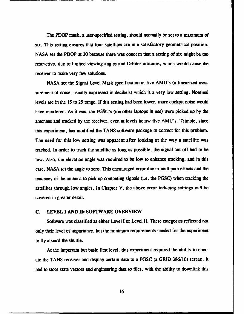
The PDOP mask, a user-specified setting, should normally be set to a maximum of
six. This setting ensures that four satellites are in a satisfactory geometrical position.
NASA set the PDOP at 20 because there was concern that a setting of six might be too
restrictive, due to limited viewing angles and Orbiter attitudes, which would cause the
receiver to make very few solutions.
NASA set the Signal Level Mask specification at five AMU's (a linearized mea-
surement of noise, usually expressed in decibels) which is a very low setting. Nominal
levels are in the 15 to 25 range. If this setting had been lower, more cockpit noise would
have interfered. As it was, the PGSC's (the other laptops in use) were picked up hy the
antennas and tracked by the receiver, even at levels below five AMU's. Trimble, since
this experiment, has modified the TANS software package to correct for this problem.
The need for this low setting was apparent after looking at the way a satellite was
tracked. In order to track the satellite as long as possible, the signal cut off had to be
low. Also, the elevatioai angle was required to be low to enhance tracking, and in this
case, NASA set the angle to zero. This encouraged error due to multipath effects and the
tendency of the antenna to pick up competing signals (i.e. the PGSC) when tracking the
satellites through low angles. In Chapter V, the above error inducing settings will be
covered in greater detail.
C. LEVEL I AND H: SOFTWARE OVERVIEW
Software was classified as either Level I or Level II. These categories reflected not
only their level of importance, but the minimum requirements needed for the experiment
to fly aboard the shuttle.
At the important but basic first level, this experiment required the ability to oper-
ate the TANS receiver and display certain data to a PGSC (a GRID 386/10) screen. It
had to store state vectors and engineering data to files, with the ability to downlink this
16
data. The downlink capability was important should a situation arise when the astronaut
crew required troubleshooting assistance from ground experts during the flight.
At the more advanced level, Level II, NASA desired some additional capability,
such as the ability to input an Orbiter state vector either manually or automatically to
compare the GPS state vector measurement to the Orbiter's. NASA also wanted to com-
pare the TANS GPS measurements with another GPS receiver used on the STS-51 pay-
load, ORFEUS-SPAS. One of the primary missions for STS-51 was to carry this
German-made satellite into space, release it to operate independently for several days,
and then rendezvous to recover it prior to returning home. The NASA engineers saw this
as an opportunity to study the relative GPS technique.
At a minimum, NASA wanted to collect the GPS data via the TANS receiver for
postflight studies. Ultimately, even after both Levels I and II were fully developed, this
GOOD test was only an experiment (or DTO). It was to be operated by the STS-51 crew
on a not-to-interfere basis, only. An example of interference occurred during the rendez-
vous with the ORFEUS-SPAS, which was one of the specified phases of flight to record
information for postflight study. The TANS experiment could not be run because the
antennas, strapped in the windows, adversely blocked the crew's view for rendezvous
and as a safety of flight concern interfered with the crew and their duties.
D. LEVEL I: SPECIFICS
Available in the Level I software were four interface displays. One display showed
the user a current TANS configuration set-up. A second display was used to send com-
mands and requests to the TANS receiver. A third showed the Orbiter's location on a
world map, and the forth display showed data for crew monitoring. This data consisted
of six rows of information for six channels and their related channel ID, satellite ID,
acquisition flag, ephemeris flag, azimuth, elevation, and doppler.
17
Also provided to the user was position and velocity in two different coordinate sys-
tems. The TANS receiver made measurement calculations using WGS-84. Its output for
position and velocity in this frame was either in cartesian coordinates or latitude, longi-
tude, and altitude. A non-trivial coordinate transformation was performed on the WGS-
84 position and velocity to translate them into one of the key reference frames used by
the Orbiter, M50.
E. LEVEL H: SPECIFICS
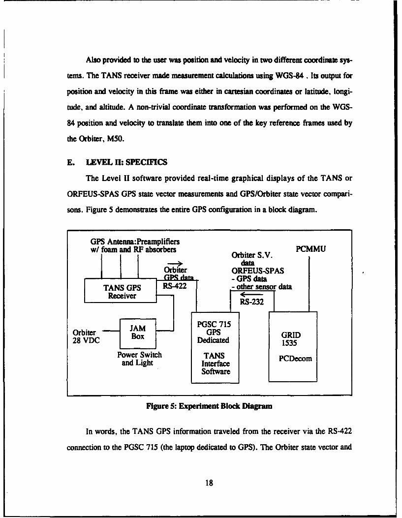
The Level II software provided real-time graphical displays of the TANS or
ORFEUS-SPAS GPS state vector measurements and GPS/Orbiter state vector compari-
sons. Figure 5 demonstrates the entire GPS configuration in a block diagram.
GPS Antenna:Preamplifiers
w/ foam and RF absorbers Oi S.V. PCMMU
-30 dataOrbiter ORFEUS-SPASSP -ja GPS data
TANS GPS R422- other sensor dataReceiver RS-232
OrbterJAM PGSC 715
Orbiter GPS GRID28 VDC Dedicated 1535
Power Switch TANS PCDecomand Light Interface
Software
Figure 5: Experiment Block Diagram
In words, the TANS GPS information traveled from the receiver via the RS-422
connection to the PGSC 715 (the laptop dedicated to GPS). The Orbiter state vector and
18
ORFEUS-SPAS GPS data traveled from the PCMMU via another GRID 1535 laptop
running the PCDecom program through the RS-232 connection to the PGSC 715 to be
manipulated in the Level II code. Part of the manipulation designs were to use the Orbit-
er's GPS (from TANS) and ORFEUS-SPAS GPS state vectors in a rendezvous program.
Much of the Level II code was written by the NPS team, with major guidance and
assistance from a computer programming wizard, and author of the PCDecom program,
Mr. Tom Silva. Greater detail about the flight code and mathematical derivations is sup-
plied in the theses written by LT Lee Barker and LT Les Makepeace.
19
I1L STATE VECTOR DIUENCING
A. DATA ANALYSIS
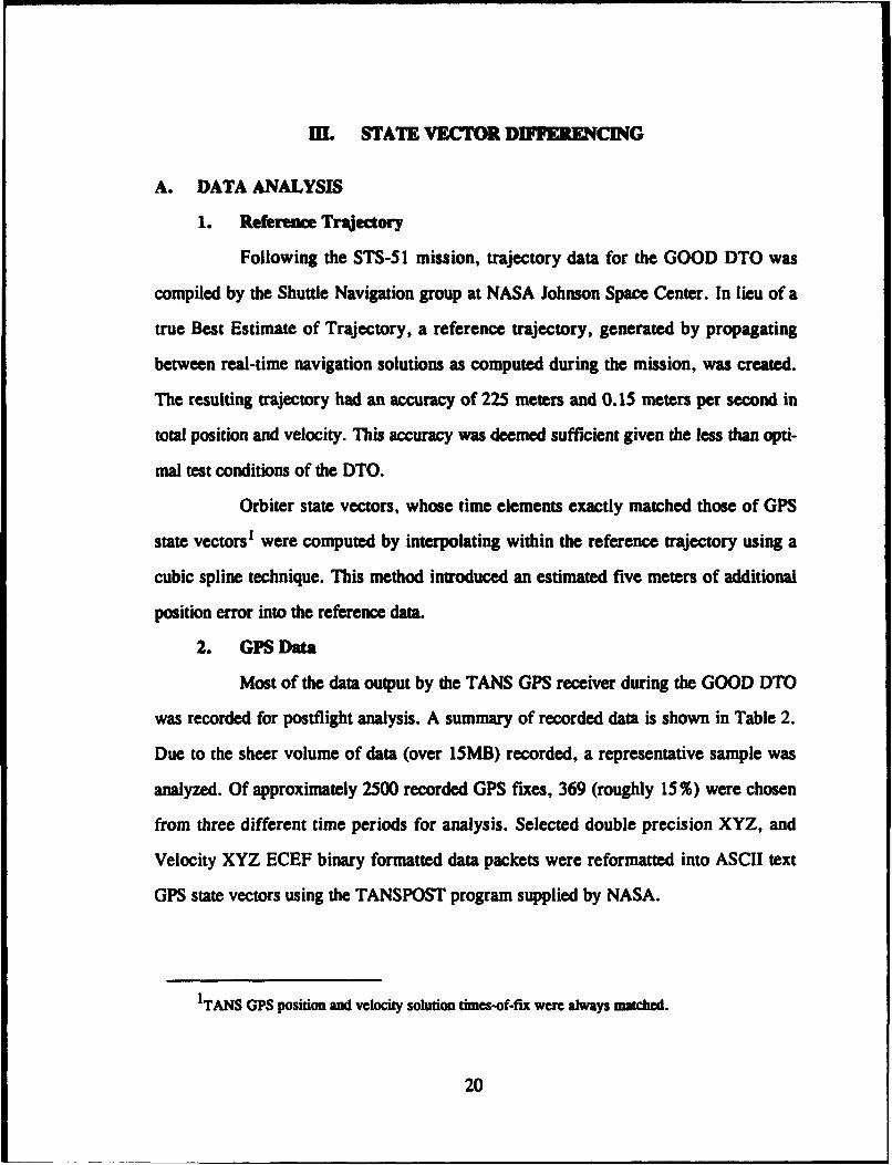
1. Reference Trajectory
Following the STS-51 mission, trajectory data for the GOOD DTO was
compiled by the Shuttle Navigation group at NASA Johnson Space Center. In lieu of a
true Best Estimate of Trajectory, a reference trajectory, generated by propagating
between real-time navigation solutions as computed during the mission, was created.
The resulting trajectory had an accuracy of 225 meters and 0.15 meters per second in
total position and velocity. This accuracy was deemed sufficient given the less than opti-
mal test conditions of the DTO.
Orbiter state vectors, whose time elements exactly matched those of GPS
state vectors1 were computed by interpolating within the reference trajectory using a
cubic spline technique. This method introduced an estimated five meters of additional
position error into the reference data.
2. GPS Data
Most of the data output by the TANS GPS receiver during the GOOD DTO
was recorded for postflight analysis. A summary of recorded data is shown in Table 2.
Due to the sheer volume of data (over 15MB) recorded, a representative sample was
analyzed. Of approximately 2500 recorded GPS fixes, 369 (roughly 15%) were chosen
from three different time periods for analysis. Selected double precision XYZ, and
Velocity XYZ ECEF binary formatted data packets were reformatted into ASCII text
GPS state vectors using the TANSPOST program supplied by NASA.
1TANS GPS position and velocity solution times-of-fix were always matched.
20
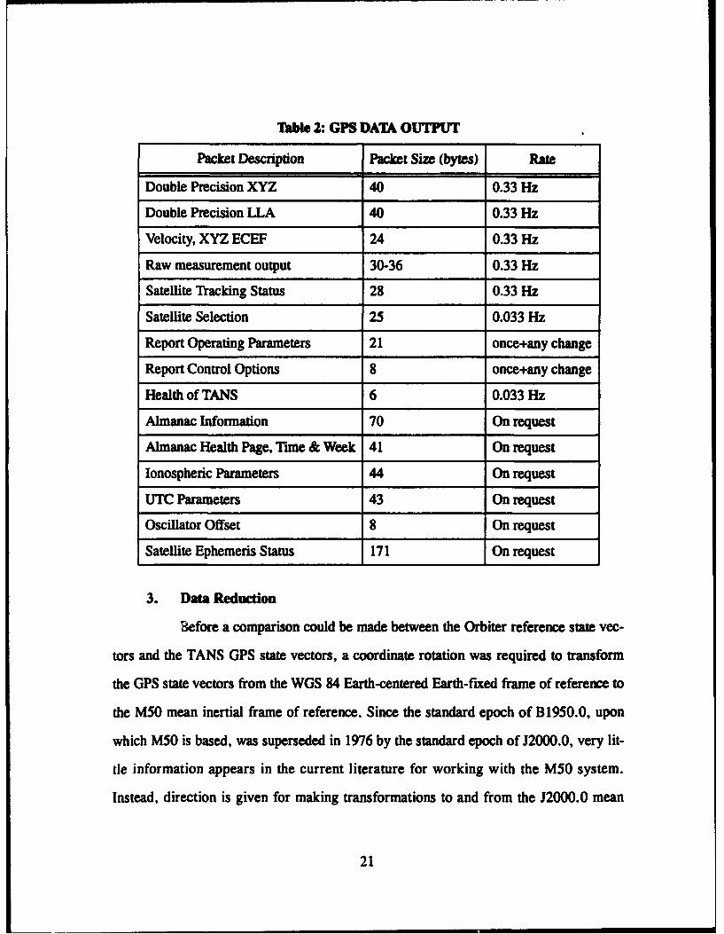
Table 2: GPS DATA OUTPUT
Packet Description Packet Size (bytes) Rate
Double Precision XYZ 40 0.33 Hz
Double Precision LLA 40 0.33 Hz
Velocity, XYZ ECEF 24 0.33 Hz
Raw measurement output 30-36 0.33 Hz
Satellite Tracking Status 28 0.33 Hz
Satellite Selection 25 0.033 Hz
Report Operating Parameters 21 once+any change
Report Control Options 8 once+any change
Health of TANS 6 0.033 Hz
Almanac Information 70 On request
Almanac Health Page, Tune & Week 41 On request
Ionospheric Parameters 44 On request
UTC Parameters 43 On request
Oscillator Offset 8 On request
Satellite Ephemeris Status 171 On request
3. Data Reduction
Before a comparison could be made between the Orbiter reference state vec-
tors and the TANS GPS state vectors, a coordinate rotation was required to transform
the GPS state vectors from the WGS 84 Earth-centered Earth-fixed frame of reference to
the M50 mean inertial frame of reference. Since the standard epoch of B1950.0, upon
which M50 is based, was superseded in 1976 by the standard epoch of J2000.0, very lit-
tle information appears in the current literature for working with the M50 system.
Instead, direction is given for making transformations to and from the J2000.0 mean
21
inertial coordinate system. While NASA continues to utilize older transformation theory
to convert Earth-centered Earth-fixed coordinates directly to MS0, the authors chose to
make the transformation first into the J2000.0 mean inertial system, and then into the
MS0 mean inertial system using a constant transformation matrix published by NASA
Jet Propulsion Laboratory (Standish, 1982, pp. 297-302) to relate the M50 and J2000.0
systems. The transformation into J2000.0 allowed the use of the newer 1980 IAU theory
of nutation for improved accuracy.
4. Coordinbt Trfsformuadin
The WGS 84 system is more accurately referred to as a geopotential model
that has adopted the Conventional Terrestrial System (CTS) (1984.0), defined by the
Bureau International de l'Heure, as its reference frame. Earth's center of mass is the ori-
gin of the CTS, as well as the M50 and J2000.0 systems. The Z-axis of the CTS is
known as the Conventional Terrestrial Pole (CTP). The X-axis of the CTS is the Zero
meridian, and is used to derive Universal Time, specifically UTI, in the same way the
Greenwich meridian is used to derive GMT. The Y-axis completes a right-handed coor-
dinate system. (DMA-TR-8350.2, 1987, p. 2-1)
Transformation of WGS 84 coordinates into M50 coordinates requires two
3x3 rotation matrices, each computed for the time of the state vector being transformed.
Transformation of position vectors actually requires only a single rotation matrix. Subse-
quent discussion will refer to this matrix as "matrix 1." Transformation of velocity vec-
tors, however, requires a second matrix to account for the rate of change within matrix
1. This matrix will be referred to as "matrix 2."
Matrix 1 is actually the product of five separate 3x3 matrices, premultiplied
to form a single matrix. The letters A, B, C, P, and M will be used to denote these five
matrices. A applies two rotations for polar motion. B applies a single rotation for side-
real time (Earth rotation). C applies three rotations for astronomic nutation. P applies
22
three rotations for general precession, and M applies three rotations for standard epoch
conversion. All matrices with the exception of M are time varying. The M50 position
vector is the product of the transpose of matrix 1, and the WGS 84 position vector.
Matrix 2 is also the product of five separate 3x3 matrices. Four of the matri-
ces used to compute matrix 1, A, C, P, and M, are also used for matrix 2. Unlike the
other time varying matrices, the rate of change of the B matrix is significant; so another
matrix, denoted by h, replaces the B matrix in matrix 2. h is the rate of change of the B
matrix. The M50 velocity vector is computed in three steps. In step one, the product of
the transpose of matrix 2 and the WGS 84 position vector is computed. In step two, the
product of the transpose of matrix 1 and the WGS 84 velocity vector is computed. In
step three, the two resulting vectors are added vectorially to form the M50 velocity vec-
tor. The transformation methodology for position coordinates is shown in Equation 1
and the transformation methodology for velocity coordinates is shown in Equation 2.
XZM = [ABCPM]T [xyz]w0 5 . (Eq: 1)
6 [3]xYZ]ws + [ABCPWS (Eq: 2)
Methods for computing the A, B, A, C, and P matrices were taken from The
Astronomical Almanac, The Explanatory Supplement to the Astronomical Almanac, and
Defense Mapping Agency Technical Report 8350.2. These methods are summarized in
sub-paragraphs a through d.
a. Polar Motion
Polar motion parameters, xp and yp, for the dates encompassing the
STS-51 mission, were obtained from the U.S. Naval Observatory. The A matrix consists
of a rotation about the Y-axis by angle -xp, and a rotation about the X-axis by angle -yp.
23
The maximum amplitude of these parameters is approximately 0.3 arc seconds. This
corresponds to about 10 meters of position difference at Shuttle altitudes.
b. Sidreal T7h
The B matrix consists of one rotation about the Z-axis by an angle of
A, where A = H0 + AH +wo*( t -At ). Ho is Greenwich Mean Sidereal Time (GMST) at
Ol UTI on the day of interest. Since 1984, GMST has been defined by Equation 3,
where T. is the number of centuries elapsed since 12h UTI on 2000 January 1. The
result is in units of seconds of sidereal time, and may be converted to arc on the basis of
one revolution per 24 hours of sidereal time.
GMST1 of hUTI = 24110.54841 + 8640184.812866T. + 0.09310472 - 6.2 x 10⁶•7(Eq: 3)
All is the Equation of the Equinoxes. It equals arctan( cose tanAW ),
where e is true obliquity of the ecliptic, and AW is nutation in longitude. Both e and AV
are computed in the course of generating the C matrix. (0* is the Earth rotation rate in a
precessing reference frame, and is equal to co' + m, where coW is the Earth's inertial rota-
tion rate, a constant, and m is equal to 7.086 x 10⁻¹² + 4.3 x 10⁻¹⁵Tu. Time t is the time
of the state vector being transformed in seconds since the beginning of the day UTC, and
At is the difference between UTI and UTC. Values of UTI minus UTC were obtained
from the U.S. Naval Observatory for the dates encompassing the STS-51 mission. These
values are kept below 0.7 seconds through introduction of leap seconds into UTC. One
second of time corresponds to 15 arc seconds, or about 485 meters of position difference
at Shuttle altitudes.
(1) Change in Sidereal Time Matrix. The A matrix is defined as
shown in Equation 4.
24
--o) sinA (o cosA 0- osA -* sinA (Eq: 4)
0 ~0 0
C. Asfrtiomi Nutadin
The C matrix consists of a rotation about the X-axis by angle e, fol-
lowed by a rotation about the Z-axis by angle -A.V, followed by a rotation about the X-
axis by angle -z. Angle e is mean obliquity of the ecliptic, and is defined by Equation 5,
where T is the number of Julian centuries elapsed since fundamental epoch J2000.0 in
barycentric dynamical time. The result is in units of arc seconds.
e = 84381.448 - 46.815T- 0.00059 72+ 0.001813 73 (Eq:5)
AV is nutation in longitude, and is defined by Equation 6, where A1,
Bi, all, a2i, a3i, a4i, and a5i are constants from the 1980 IAU nutation series, shown in
Table 3.222.1 of the Explanatory Supplement to the Astronomical Almnane, and 9, r, F,
D, and Q are fundamental arguments of the 1980 IAU theory of nutation. The result of
nutation in longitude is in units of 0.0001 arc seconds.
106
A = (Ai+BiT) sin (alit+a 2it'+a 3iF+a 4iD+a 5 il) (Eq: 6)
The fundamental arguments are depicted in Equations 7 - 11. The
superscript r represents revolutions, and results are in units of arc seconds.
= 485866.733 + (1325r + 715922.633) T+ 31.3172 + 0.064T3 (Eq: 7)
= 1287099.804 + (99r + 1292581.244) T- 0.577T2 - 0.012T73 (Eq: 8)
25
F = 335778.877 + (1342' +295263.137) T- 13.257T 2 +0.011T 3 (Eq: 9)
D = 1072261.307 + (1236r + 1105601.328) T- 6.891T 2 + 0.0197T (Eq:10)
Q = 450160.28 - (5r +482890.539) T+ 7.45572 + 0.008T 3 (Eq:11)
Angle e is ue obliquity of the ecliptic, and is equal to Z +Ae, where
Ae is nutation in obliquity. Ae is defined by Equation 12, where Ci and Di are additional
constants from the 1980 IAU nutation series, found in table 3.222.1 of the Explanatory
Supplement to the Astronomical Almanac. The result of nutation in obliquity is in units
of 0.0001 arc seconds.
106
A= (Ci + DT7) cos (aul+a 21t'+a 3iF+a 4iD+ asit) (Eq:12)i-I
(1) More Accurate Nutation. Aic and AEC are corrections to be
added to the 1980 IAU nutations in longitude and obliquity, AV and Ae, respectively.
AVc and Aec are defined by Equations 13 and 14, where LSn, LCn, OCn and OS, are
constants from the corrections to IAU 1980 nutation series given in table 3.224. 1 of the
Explanatory Supplement to the Astronomical Almanac. The results of these nutation cor-
rections are in units of 0.00001 arc seconds.
4
Avc = 7a (LSnsinAn+LCncosAn) (Eq:13)n=l
4
AeS = E (OCncosAn +OSnsinAn) (Eq:14)
n--
26
An is equal to ant + bnC +c8 + dnD + e, 1f, where an, ba, cn, dn,
and en are additional constants from the corrections to the 1980 IAU nutation series
given in table 3.224.1 of the Explanatory Supplement to the Astronomical Almanac.
d. General Preceusion
The P matrix consists of a rotation about the Z-axis by angle -ý, fol-
lowed by a rotation about the Y-axis by angle 0, followed by a rotation about the Z-axis
by angle -z. Angles C, 0, and z are defined by the accumulated precession angles adopted
by IAU 1976, and are shown in equations 15 - 17, respectively. The results are in units
of arc seconds.
S= 2306.2181T + 0.30188T 2 + 0.01799873 (Eq:15)
z = 2306.2181T+ 1.09468T 2 + 0.0182037 3 (Eq:16)
0 = 2004.3109T- 0.426657 - 0.04183373 (Eq: 17)
e. Standard Epoch Conversion
The M matrix is depicted in Equation 18.
0.9999256791774783 -0.0111815116768724 -0.00485900381545530.0111815116959975 0.9999374845751042 -0.0000271625775175] (Eq: 18)0.004859003771445 -0.000027170449221 0.9999881946023742_
5. Summary
The coordinate conversion process was implemented in C + + (Borland ver.
3.1). The program was run using an IBM compatible personal computer. The computer
code is included as Appendix A. The code's accuracy was validated in two ways. First,
precession, nutation, and Earth rotation (sidereal time) angles as shown in the Astro-
nomical Almanac were accurately reproduced for a given date. Second, a sample set of
transformed TANS GPS coordinates produced by the program was compared with the
same set of coordinates, transformed by the Shuttle Navigation group at NASA. Radial
position differences were less than six meters (less than 0.18 arc seconds of rotation),
27
and radial velocity differences were less than 0.007 meters per second. This level of
accuracy was considered sufficient, given the differing methods used in making the
transformation.
B. NAVIGATION PERFORMANCE
Following coordinate conversion, the TANS GPS state vectors and Orbiter refer-
ence state vectors were input into a second computer program to compute the RSS posi-
tion and velocity differences. The computer code utilized is included as Appendix B.
The results for each data set were plotted, and the mean differences and standard devia-
tions were computed.
Three sets of data were chosen for analysis of the TANS GPS receiver's naviga-
tion performance. The principle criterion used in selection of these data points was the
absence of any prolonged time interval between navigation fixes for the period under
consideration. For the periods chosen, time between fixes is generally 2.5 seconds, with
occasional gaps of up to 7.0 seconds. Data recorded during the STS-51 mission was seg-
regated into files labeled A through M, 0, P, Qi, Q2, RI, R2, and S through U. In gen-
eral, the files corresponded to a particular event or activity during the mission. Large
files were subdivided into smaller files using a numerical suffix, such as P.001, P.002,
etc. The P files corresponded to the crew sleep period between flight day 6 and 7, and
contained over half the TANS GPS state vectors collected during the mission. All data
analyzed was taken from P files.
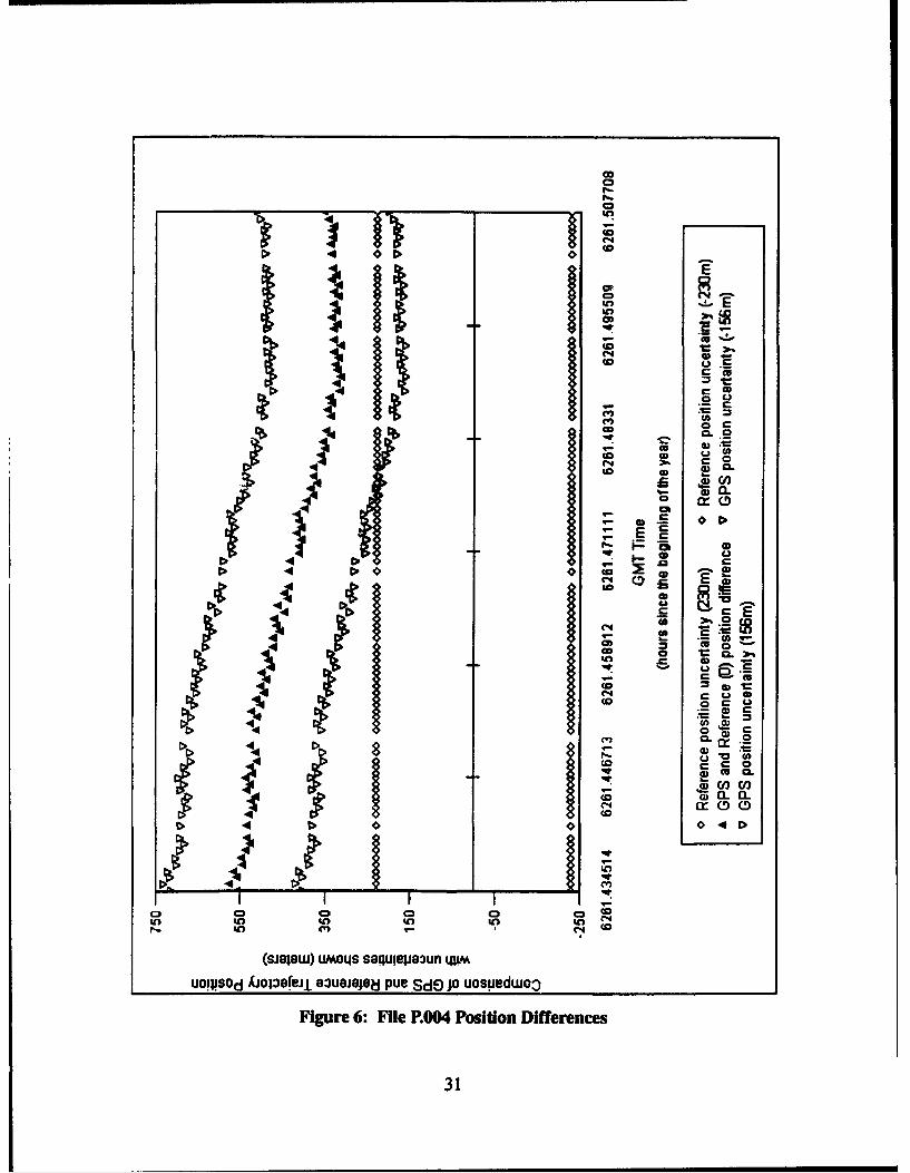
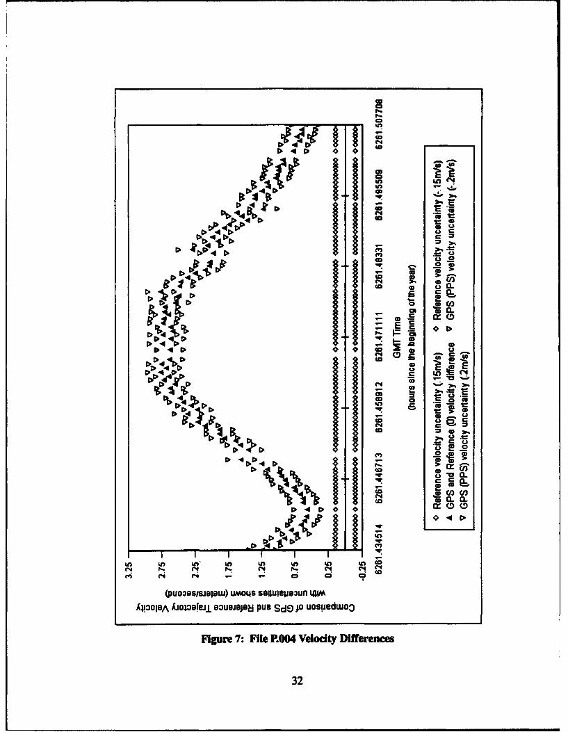
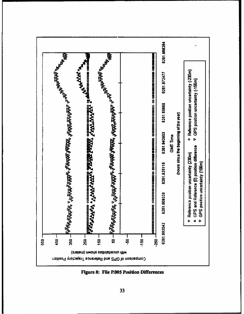
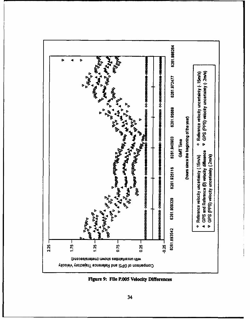
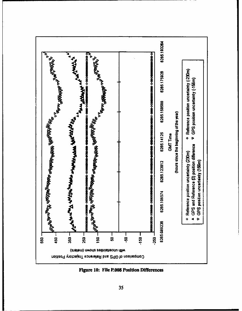
Analysis of the results is shown in Table 3, and in Figures 6 through 11. The Fig-
ures depict the magnitude of the position and velocity differences, and show the range of
error for each measurement, as well as for the reference trajectory. The times immedi-
ately preceeding, and immediately following the analyzed data were periods when the
receiver was not computing navigation solutions. In general, a fourth satellite had just
28
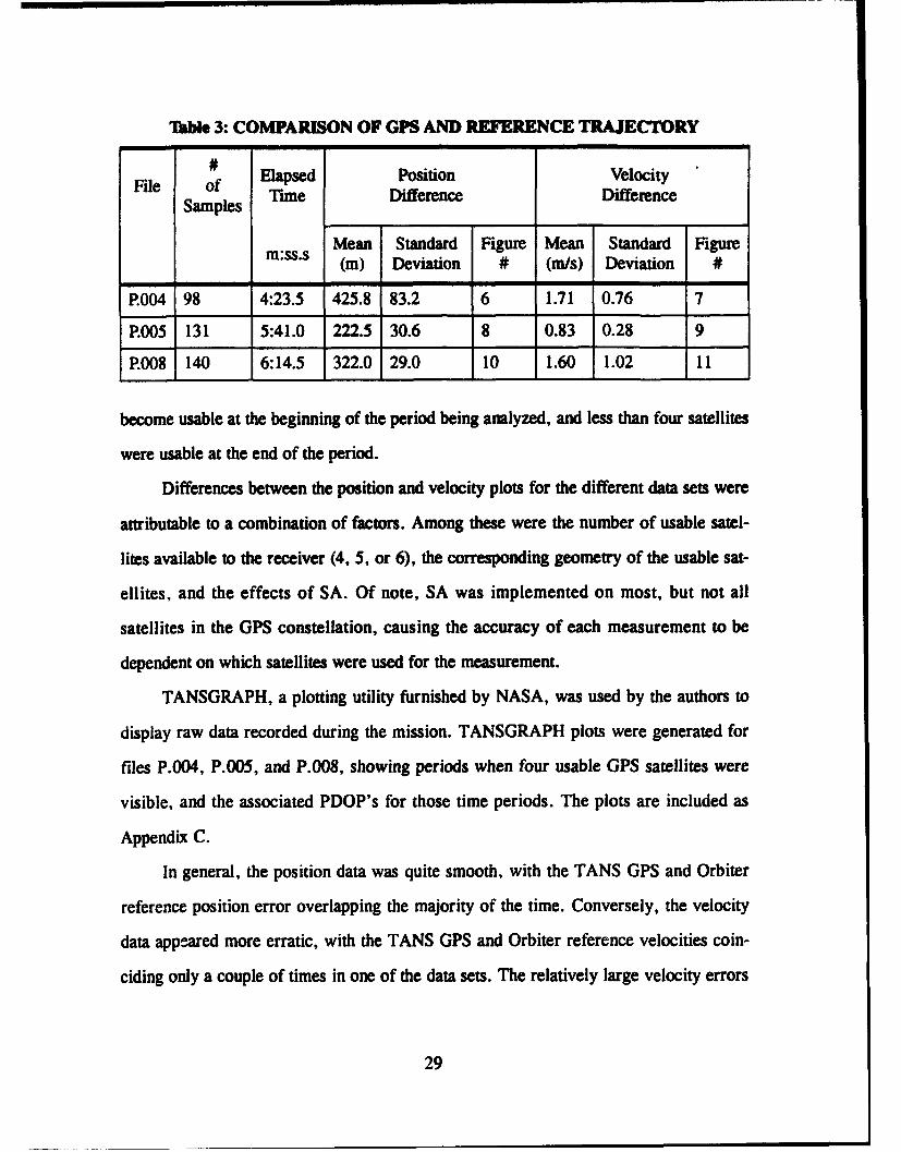
"E&be 3: COMPARISON OF GPS AND REFERENCE TRAJECTORY
File of Elapsed Position VelocitySamples Tune Difference DifferenceSamples
Mean Standard Figure Mean Standard Figurem:ss.s (m) Deviation # (m/s) Deviation #
P.004 98 4:23.5 425.8 83.2 6 1.71 0.76 7
P.005 131 5:41.0 222.5 30.6 8 0.83 0.28 9
P.008 140 6:14.5 322.0 29.0 10 1.60 1.02 11
become usable at the beginning of the period being analyzed, and less than four satellites
were usable at the end of the period.
Differences between the position and velocity plots for the different data sets were
attributable to a combination of factors. Among these were the number of usable satel-
lites available to the receiver (4, 5, or 6), the corresponding geometry of the usable sat-
ellites, and the effects of SA. Of note, SA was implemented on most, but not all
satellites in the GPS constellation, causing the accuracy of each measurement to be
dependent on which satellites were used for the measurement.
TANSGRAPH, a plotting utility furnished by NASA, was used by the authors to
display raw data recorded during the mission. TANSGRAPH plots were generated for
files P.004, P.005, and P.008, showing periods when four usable GPS satellites were
visible, and the associated PDOP's for those time periods. The plots are included as
Appendix C.
In general, the position data was quite smooth, with the TANS GPS and Orbiter
reference position error overlapping the majority of the time. Conversely, the velocity
data appeared more erratic, with the TANS GPS and Orbiter reference velocities coin-
ciding only a couple of times in one of the data sets. The relatively large velocity errors
29
would introduce significant error if used in a propagation scheme, and would be unsuit-
able for navigation purposes without some effective form of filtering. A few data points
were observed to differ from neighboring points by an anomalously large amount. It is
possible that these deviations were produced as an artifact of data recording, or data
extraction by the TANSPOST program. NASA has since incorporated a six standard
deviation rejection scheme into the GPS processing to eliminate outlying points. (Saun-
ders, 1994, pp. 1-13)
30
C3I.-
tof IUD
cci (a
W CL
00 G
CD 0 I>0
jC EC4 c '.2 to
CmC
(-4
0 tO.)8
CC C -0
1n Cn
C)f C3 C3C Cr--0 W) CO C
1 I 31
V'-
C4C4 'a
C3
DD .q C14~4~Co
(.4 bpCfl(04
0
Co a43 pcn
-C> C~o
'a b
PiD 4,4 VDio Di4 D
Di>1'" C0
C14-ic~ C1re 3DODi it (D0
VpN (N
p. (N -~ ax 0
(puoss~ssCIw .0LI sSUIlS3f 4 ODA~~~~~ogaA ~ ~ ~ ~ ~ A 4JISSiSUJJ~ U d OUSJdO
F~~gure 7:~~ FieCP.0 CAotyDferne
to32
C4
w
C4m
lCkt 4 ~.5Q
(0 0 CO
Co CU
4 0)CLC
EnM CA) ClBL
33
to4D4
0 0 0
1> 4 V.9ccC4
C'. 4 uV
h C4Q1I
1>~~ ~ ~ L6 v r4 L
3Kcc~1>
Ifl o'C4
C', 0. 4 C, )14 En
I (L-IC~ in
CIO 0 0l 1
344
C1
CV)C
4 to.
C4C
Wall
* 44CO
ccC C am
'.4 w--w.
(sjebsww UMLSSeUSi~U f4UOWSd kOsI~j 9~SJ68~ p~ Sd jouosudCL
35

C4
Ca
'.4
cc
C4
cc c
ClC
C4 a C-
_O 'a.~D
4b C4 C
Can
C C4
oio
r--
DiDQ~ 4Dncn
'a La O~o
COD
Dir
Cm~
'aU U7 Cc '4
(PU08SISJeGaw) UM04JS seqieiamnSUf qpm
iAI3019A AJOPSAJI 83USJ6J8 PUe SdE) J0 uosuedwo3
Figure 11: File P.008 Velodty Differences
36
IV. STATE VECTOR FILTERING
A. INTRODUCTION
1. The Purpose for a Filer
Chapter I discussed how a GPS receiver measures p ranges to four sat-
ellites in order to solve for a three dimensional position. The GPS receiver calculates the
user's position and GPS time by knowing the position of these four satellites from
decoding their navigation messages. Pseudorange measurements are made because the
GPS receiver can not measure the exact range to each satellite. These measurements are
corrupted by ionospheric delays, user clock drift, receiver noise and other errors. Typi-
cally a filter is used to characterize some of the noise sources in order to minimize their
effects on the navigation solution. A Kalman Filter can be used both within the receiver
logic or in a post-processed phase. Additionally, a smoothing algorithm could be applied
in the post-processing of data. Most filtering schemes studied today integrate the Kalman
Filter with the Inertial Navigation System (INS) by using external informative sources to
improve position (LORAN, OMEGA, laser ranging, etc.), velocity (Doppler radar), and
altitude (barometric, radar and laser altimeters). In this thesis, a version of the Kalman
Filter is implemented and analyzed in the post-processing phase in which user position,
velocity and GPS time are known from STS-5 l's flight. This filter is an adaptation of a
Kalman Filter program, written by Dr. Titus, a professor from the Naval Postgraduate
School, which uses seven states including position (X, Y, Z), velocity (Vx ,Vy ,VZ ),
and time (t). The theory of the Kalman Filter will be described briefly along with the
adapted computer code (see Appendix D). The final results will be analyzed to show the
effects, both positive and negative, a Kalman Filter has on this post flight data.
37
B. KALMAN FILTER
1. Tbeoritcal Model
The GPS Kalman Filter is a model of how its stain vector is changing in time
or how the host vehicle is maneuvering in time. The state vector includes parameters
which describe the model, a minimum of which is receiver position (X, Y, Z) and time.
The simplest way to describe the Kalman Filter is as a recursive estimator that produces
a minimum covariance estimate of the state vector in a least squares sense. The covari-
ance estimate or matrix expresses the statistical uncertainty in the state vector. The
uncertainty grows during long periods without measurements. However, when a new
measurement becomes available it will be weighed heavily regardless of how noisy it
may be unless the filter designer plans accordingly.
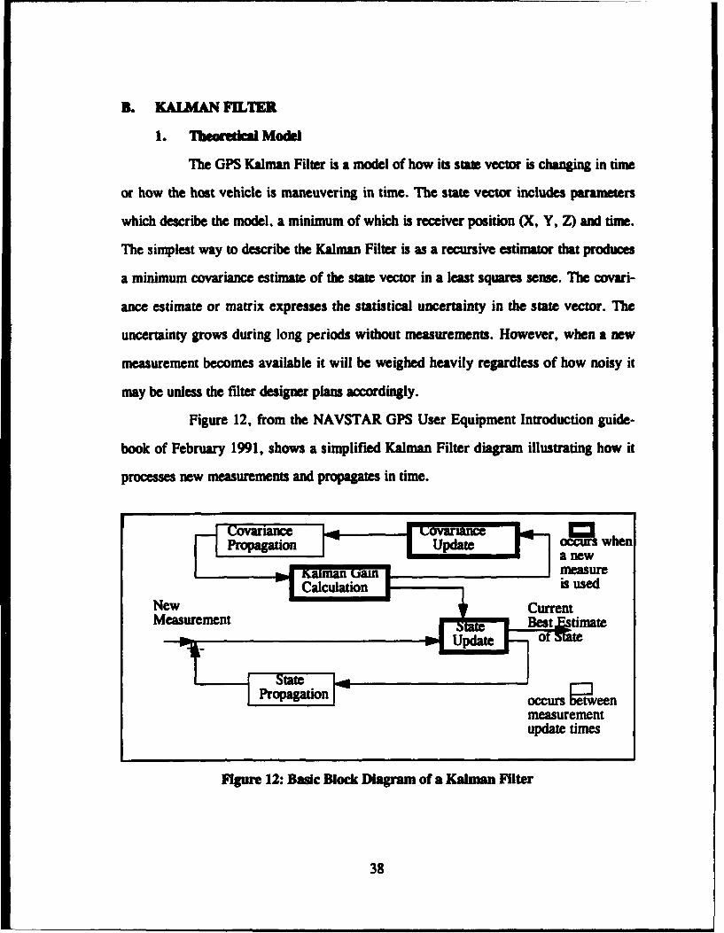
Figure 12, from the NAVSTAR GPS User Equipment Introduction guide-
book of February 1991, shows a simplified Kalman Filter diagram illustrating how it
processes new measurements and propagates in time.
"I Calculatid is usedNew ICurrent
Mesrmn state Nes occurs
Propagation owuenL
mea•surementupdate times
FIgure 12: Basc Block Diagram of a Kalman Filter
38

2. Tioedeial Euatlmon
The basic process of the discrete Kalman Filter, is to model the state vector,
Xt, as it transitions over time, from timestep to timestep. The A~ matrix is called the
measurement or observation matrix. The measurement zt vector is a function of the state
given by Ht. The following equations represent two processes, Equation 19 for state and
Equation 20 for measurement.
It= 2Mt-e A- - +E-I (Eq.19)
;t = A.t +N (Eq.20)
The 0 matrix is the transition matrix between the covariance matrix (Pd) and state (zt).
To account for the uncertainty in the state and measurement models, the noise (Gaussian
white) terms mt., and xt are included. The Kalman Filter alterntes between propagating
the state (zt) and its covariance (P) and updating these variables with new measure-
ments. The Qt matrix is the variance of the state noise and it accounts for the error in the
modeling assumptions of 0. The following equations are used to express the propagation
of the state (x.) and the covariance (Pd.
Xt 2- Owt- A- (Eq.21)
Pt =Ot-Pt-I -OTt-I + Qt-I (Eq.22)
Updating is defined as incorporating additional measurements into the filter
at regular intervals. The state immediately updated is considered to be the most optimal
state in the filter. At this point, the new measurement of the state is compared with the
propagated estimate. This difference is scaled using the Kalman Gain (IQ) and then used
in calculating the new state estimate. Symbols (-) and (+) are used to distinguish
betweer filter estimates immediately before and after a measurement. The following
equation expresses the update procedure.
It(+) = It(-) + Kt[ zt-Ht -xt(-) (Eq.23)
39
The next step is to update the covariance matrix (Pt). In Equation 24, the new meaure-
ment is weighted by dhe Kalman Gain (Kt) and differenced with the identity matrix (I).
This result determines the degree to which the covariance matrix is improved by the new
measurement.
t - [I-KtHt ] "P() (Eq.24)
Finally, some understanding of the Kalman Gain (Kt) is required. It is a
result figured each time a measurement update occurs. The calculation is not only based
upon the propagated covariance matrix of the previous time, Pt (-), but it is also upon the
current measurement noise covariance (Rd) and the sensitivity of the measurement to
small changes in the state (Ht = 8H/8St ).K~t =- Pt (-).-Wt .[Eh-Pt (-) .HITt +. Rt 1-1 (FEq.2.5)
To try to explain this equation, an example from the NAVSTAR GPS User
Equipment will be cited. First, assume that the state vector and measurement matrix are
both in the same coordinate frame so that the Ht matrix becomes the identity matrix.
Second, simplify the notation and matrix formulation to show the Kalman Gain as K =
P / (P + R), where P continues to represent the covariance and R represents the mea-
surement noise. So for a large P, or uncertainty in the model, compared to the uncer-
tainty in R, the gain applied to the new measurement is weighed heavily at almost unity.
In other words, the propagated state has too large of an uncertainty, so the new measure-
ment is seen as a better estimate and is used as such. For the other case, when there is a
large uncertainty in the measurement noise as compared to the state (i.e. R> >P), the
Kalman Gain is very small and the new questionable measurement is weighted by a small
amount.
40
C. AN ADAPTATION OF TIHE KALMAN FILTER
1. Analysis of Problem
Examining filtering for the first time, the decisions concerning what to filter
and which parameters to characterize were the most challenging aspects to this problem.
After researching Kalman Filter theory and obtaining guidance from experts in this field,
the problem, at last, became well defined. First it was necessary to study the TANS
receiver. It was important to know that Trimble had designed it to work without a filter
calculating position and velocity in a deterministic manner. The advantage of accessing
this information without previous filtering schemes is that it allows one to create several
filtering designs post-flight, having knowledge of the data's behavior. Without access to
the original pseudorange and pseudorate information, the problem became one of filter-
ing the output of the receiver using the position (X, Y, Z), velocity (Vx, Vy, Vz) and
time (t) parameters. A more elaborate filter might use other parameters, such as, GDOP,
Carrier to Noise, and accelerations to assist in weighing new measurements.
Throughout the entire STS-51 flight, there were twenty two periods of
TANS GPS operation. Table 4, on the following page, is a modified table from "The
First Flight Tests of GPS on the Space Shuttle." It is presented as a reference to show
experiment operation periods, Shuttle activity, and related satellite tracking statistics.
After plotting raw position and velocity data, as seen in Chapter III, it was
evident that the position solutions tracked smoothly without applying filtering tech-
niques. Choosing one of the P files, GPSS1P.O05, provided an acceptable base from
which to study the Kalman Filter and analyze its advantages and disadvantages. How-
ever, to carry the navigation process through potentially long gaps of measurements
required a more elaborate filtering scheme not addressed here.
41
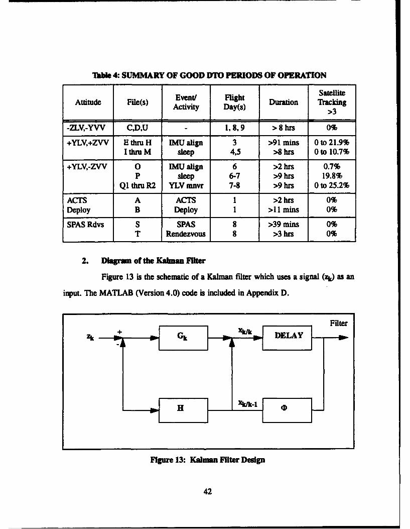
Thl 4: SUMMARY OF GOOD DTO PERIODS OF OPERATION
SatelliteAttitude File(s) Activity Day(s) Duration TrackingA D>3
-ZLV,-YVV CD,U 1,8,9 > 8 hrs 0%
+YLV,+ZW EthruH IMU align 3 >91 mins 0 to 21.9%I thru M sleep 4,5 >8 hrs 0 to 10.7%
+YLV,-ZVV 0 IMU align 6 >2 hrs 0.7%P sleep 6-7 >9 hrs 19.8%
Q1 thru R2 YLV mnvr 7-8 >9 hrs 0 to 25.2%
ACTS A ACTS 1 >2 hrs 0%Deploy B Deploy 1 >11 mins 0%
SPAS Rdvs S SPAS 8 >39 mins 0%T Rendezvous 8 >3 hrs 0%
2. Dagram of the Kalman Fiter
Figure 13 is the schematic of a Kalman filter which uses a signal (zt) as an
input. The MATLAB (Version 4.0) code is included in Appendix D.
Filter
H (
FIgure 13: Kalman Filter Design
42
3. Decripdon of the Kaim M er Dedig•
The signal input to the filter consists of the current position, velocity, and
time. The Gk is a n x m matrix representing the Kalman Gain. H is an m x n measure-
ment or observation matrix which isolates selected states. Pk/k and Pk/k-1 are square
matrices [2 x 2] representing the covariance of error of the estimator at k given k obser-
vations and at k given k-I observations, respectively. The R matrix (m x m) is the cova-
riance matrix of the measurement noise and Q (1 x 1) is the covariance of the signal
excitation.
The following formulas are used in this Kalman Filter design.
Gk = Pk/k-I HT[HPk/k-1HT + R]"1 (Eq.26)
Pk•= = [I - GkH1 PIA- 1 (Eq.27)
Pk+I/k =--PkkOT + Q (Eq.28)
These Kalman Filter equations provide the gains (G) for a typical tracking filter as listed
below.
XM = 4A- + Gk [Zk - Hz•.-1 (Eq.29)
where
%k-I = D Xk.-1/k.-1 (Eq.30)
H = [10OJ
x•fixkk I (+ (Cy- Xk/&-1) (Eq. 31)Lou Xklk- [g2(t)]
At the first observation, when k = 1,
XI/O = 0, g(1) = 1, g2(1) = 0
43
At the second observation, when k =2, then gi(2) =I and g2 (2) = I/T (noise free).
From the third observation on, the gains will decrease asymptotically to steady state val-
ues which depend upon the ratio of the appropriate term of the excitation covariance (Q)
and associated measurement noise variance (R).
D. RESULTS FROM USING A KALMAN FILTER
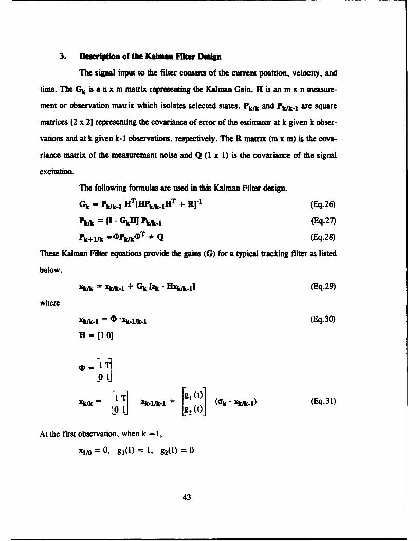
In the next few pages, plots generated using MATLAB are analyzed to show how
well this simple filter performed. Beginning with a look at the behavior of the unfiltered
data, it is clew, that this series of data illustrates relatively smooth information. Figure 14
and Figure 15 show the Z position and V. (velocity in the Z direction, termed Z dot) as
compared to their estimate, Zhat, generated using the Kalman Filter. The connecting
line shows the unfiltered position and velocity data. The position plot, Figure 14, uses
the "+" symbol to identify the filtered position estimate. The velocity plot, Figure 15,
uses the "o" to discretely show the trend of the filter and one notices the bias in this plot
until Q and R are fine tuned. In both of these figures, Q =0.01 and R =1.
X 106 Real vs Predicted in Z using 0=0.01 and R-1.2.2
A-2.6
N -2.8
C
-3.23200 3250 3300 3350 3400 3450 3500 3550
seconds
FIgure 14: Z Position - Real (-) vs Predicted (+)
44
2000
1'500 _ _ __ _ _ _ _ _
3200 3250 3300 3350 3400 3450 3500 3550time in seconds
Figure 15: Velocity in Z Direction - Real (-) vs Predicted (o)
In the figures above, one sees that after approximately five inputs, the filter stead-
ies and maintains a track at that level. This characteristic highlights a major issue con-
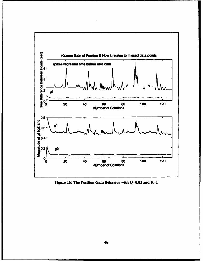
cerning this filter, initialization. Without initialization, the filter generates a spike. After
fine tuning the noise characteristics of Q and R, the spike in some magnitude remains.
Figures 16 and 17 demonstrate the initialization jump for both position and velocity. In
order to emphasize the spike, these figures use Q =0.01 and R = 1. In Figure 16, the
topmost plot on the following page, the discrete time jumps are plotted against the posi-
tion gain behavior to show that the time steps are not constant (an average time step of
2.5 ;econds with seven seconds being the greatest step) and correlate the changes in time
step with the gain changes. With a longer step than 2.5 seconds, one can see the gain
increase as it wants to weigh the "overdue" measurement more than its own propagated
state.
45
Kalman Gain of Position & How It relates to missed data points
S0 20umber o 80Sol0tionI I I - I I I ,
*12
to
0 20 40 60 80 100 120Number of Solutons
Figure 16: The Position Gain Behavior with Q--0.0I and R=1
46
%0e6
Kaklan Gahi of Velocity wfth 0=0.01 and R=1
0.25
0.2a
80.15
0.1
0.05 9
00 20 40 60 s0 100 120
Number of Solutions
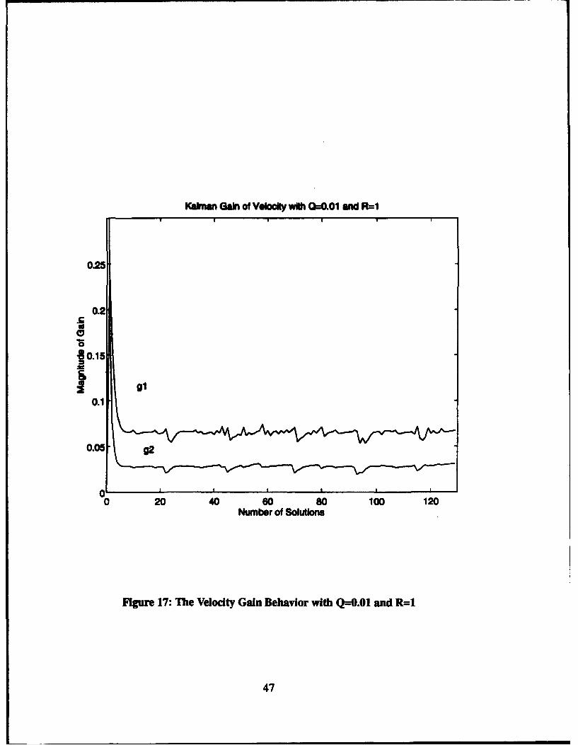
Figure 17: The Velocity Gain Behavior with Q=O.01 and R=I
47
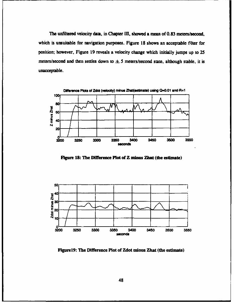
The unfiltered velocity data, in Chapter III, showed a mean of 0.83 meters/second,
which is unsuitable for navigation purposes. Figure 18 shows an acceptable filter for
position; however, Figure 19 reveals a velocity change which initially jumps up to 25
meters/second and then settles down to .-± 5 meters/second state, although stable, it is
unacceptable.
Difference Plots of Zdot (velocity) minus Zhat(estdmat) using "=0.01 and R=1100
N
01
figure 18: The Difference Plot of Z minus That (the estimate)
530
E40
3200 3250 3300 3350 3400 3450 3500 3550
seconds
igure9 1: The Difference Plot of Zdot minus Zhat (the estimate)
48
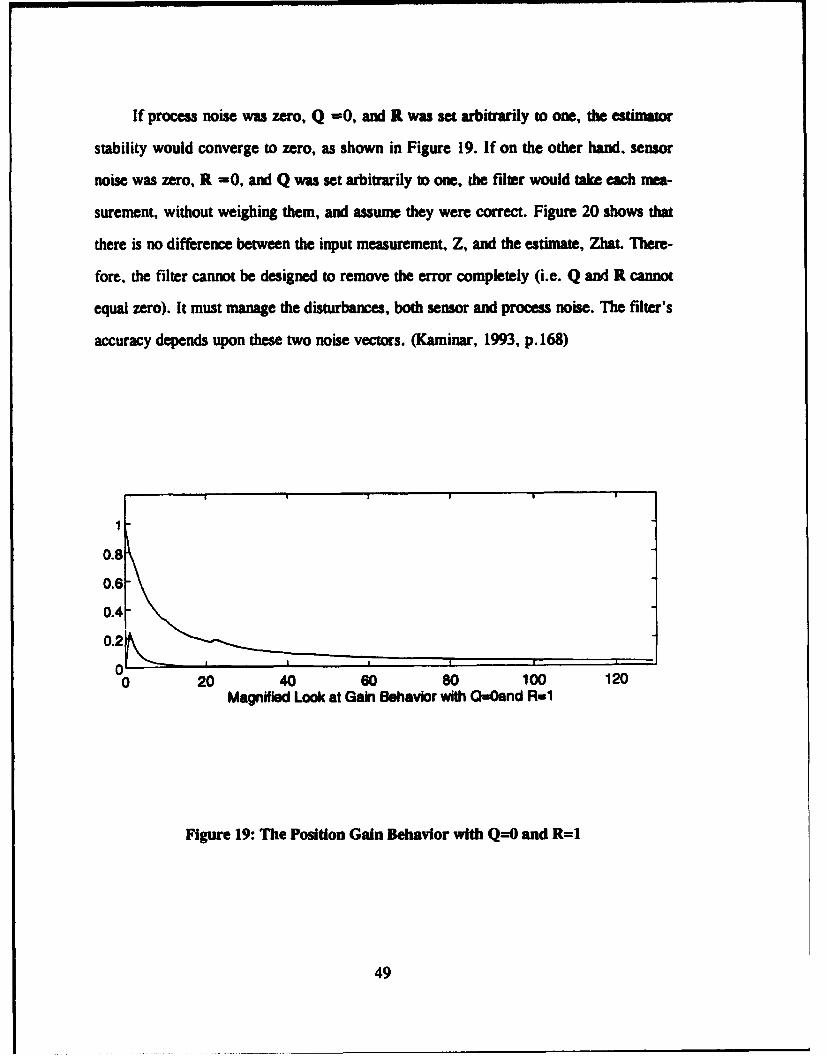
If process noise was zero, Q =0, and R was set arbitrarily to one, the estimator
stability would converge to zero, as shown in Figure 19. If on the other hand, sensor
noise was zero, R =0, and Q was set arbitrarily to one, the filter would take each mea-
surement, without weighing them, and assume they were correct. Figure 20 shows that
there is no difference between the input measurement, Z, and the estimate, Zhat. There-
fore, the filter cannot be designed to remove the error completely (i.e. Q and R cannot
equal zero). It must manage the disturbances, both sensor and process noise. The filter's
accuracy depends upon these two noise vectors. (Kaminar, 1993, p. 168)
0.8
0.60.4
0.2ýI
0 20 40 60 80 100 120Magnified Look at Gain Behavior with Q-=Ond R-1
Figure 19: The Position Gain Behavior with Q--0 and R=1
49
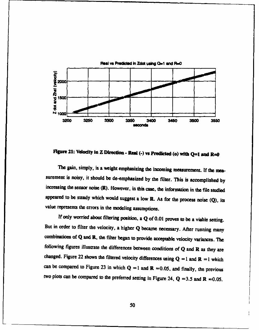
R@el vs Predhid in Zdt usin Oul and R•O
2000O
1500C
3200 3250 3300 335 3400 3450 acM 3550
Figure 21: Vdodty in Z Direction - Real (-) vs Predicted (0) with Q=1I and Ru0
The gain, simply, is a weight emphasizing the incoming measurement. If the mea-surement is noisy, it should be de-emphasized by the filter. This is accomplished byincreasing the sensor noise (R). However, in this case, the infortmation in the file studiedappeared to be steady which would suggest a low R. As for the process noise (Q), its
value represents the errors in the modeling assumptions.
If only worried about filtering position, a Q of 0.01 proves to be a viable setting.But in order to filter the velocity, a higher Q became necessary. After running manycombinations of Q and R, the filter began to provide acceptable velocity variances. Thefollowing figures illustrate the differences between conditions of Q and R as they arechanged. Figure 22 shows the filtered velocity differences using Q = 1 and R = 1 whichcan be compared to Figure 23 in which Q = 1 and R =0.05, and finally, the previoustwo plots can be compared to the preferred setting in Figure 24, Q =3.5 and R =0.05.
50
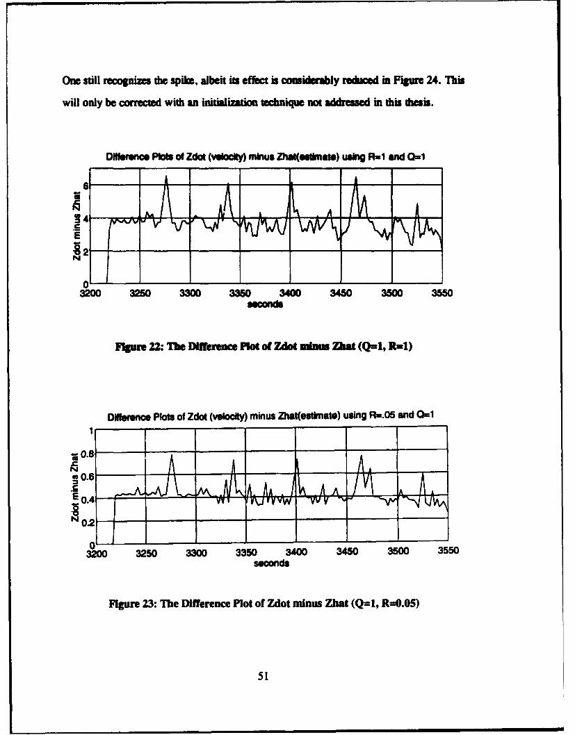
One still recognizes the spk, albeit its effect is Considerably reduced in Figre 24. "his
will only be corrected with an initialization technique not addressed in this thesis.
Difference Plots of Zdot (vecW) minus Zhat(esimate) using RuI and 0C,1
6 A
Figure 22: Th~e Diff'erene P~lot of Ziot ninuu Th (Q=1, R=I)
Difference Plots of Zdot (velocity) minus Zhat(estlnate) using FR,..0 and 0-1
O.5
N _______
E 0.
3200 3250 3300 3350 3400 3450 3500 3550seconds
Figure 23: The Difference Plot of Zdot minus Zhat (Q=1, R=1.05)
51
N A
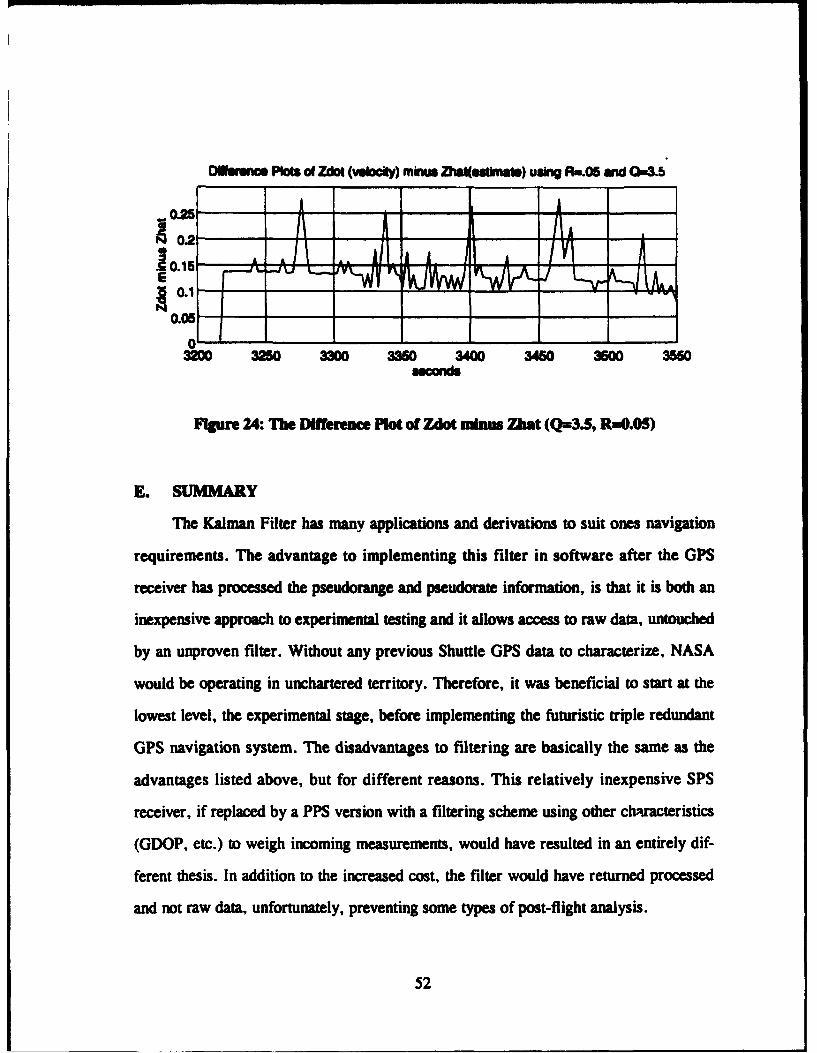
Dlhwmc P•o c Zdot (vebciy) mius iZat(.h ) usng F..06 an Q.3
0.1
0.05
03200 3250 3300 3360 3400 3460 3500 3550
Figure 24: The Difference Plot of Zdot ninhm Zhat (Q=3.5, R=0.05)
E. SUMMARY
The Kalman Filter has many applications and derivations to suit ones navigation
requirements. The advantage to implementing this filter in software after the GPS
receiver has processed the pseudorange and pseudorate information, is that it is both an
inexpensive approach to experimental testing and it allows access to raw data, untouched
by an unproven filter. Without any previous Shuttle GPS data to characterize, NASA
would be operating in unchartered territory. Therefore, it was beneficial to start at the
lowest level, the experimental stage, before implementing the futuristic triple redundant
GPS navigation system. The disadvantages to filtering are basically the same as the
advantages listed above, but for different reasons. This relatively inexpensive SPS
receiver, if replaced by a PPS version with a filtering scheme using other ch~uacteristics
(GDOP, etc.) to weigh incoming measurements, would have resulted in an entirely dif-
ferent thesis. In addition to the increased cost, the filter would have returned processed
and not raw data, unfortunately, preventing some types of post-flight analysis.
52
V. ERROR SOURCES
A. PREDOMINANT ERROR SOURCES
In Chapters II and IV, several errors were addressed briefly; however, in this
chapter an exhaustive list will be discussed. The major error in the navigation solution is
generated from the DOD's use of Selective Availability (SA). System accuracy may be
degraded by DOD, to fixed levels by dithering (a method of moving the locations of the
bits about in time using a technique "authorized users" may remove). The current policy
implements SA at a level giving a 100 meter horizontal (two standard deviation) error.
This intentional error is the largest one and has the greatest impact. Although other
errors are addressed, unless a method such as differential or relative GPS is incorpo-
rated, or a PPS receiver is utilized, these smaller errors control less than one half the
magnitude of the total error. The additional errors which will be addressed are atmo-
spheric delays, clock differences, ephemeris error, multipath, receiver noise, and Dilu-
tion of Precision (DOP).
Atmospheric delay is caused by the ionosphere and troposphere. The ionosphere is
a layer of free electrons and ions above the atmosphere from approximately 100 km to
1000 km. Pseudoranges are significantly lengthened because these charged particles
slow transmissions from the GPS satellites. The amount of distortion is directly propor-
tional to the number of electrons along the transmission path. The error can range from
5 to 40 meters, depending on the scenario. For example, a low elevation angle to the sat-
ellite affects the signal more than an overhead view.
Four additional factors affect the electron concentration in the ionosphere. They
are the solar cycle, time of year, time of day, and latitude. The sun follows an 11 year
cycle with the next peak predicted to occur around the year 2001 to 2002 which will
53
have its maximum influence on the ionosphere. Spring equinox brings the greatest sea-
sonal levels of electron concentration. The most active time of the day is at 1400 local
time as compared to night when the ionosphere causes its least interference. To eliminate
errors due to the ionosphere, the preferred method is to use both the Li and L2 carrier
frequencies, since its effect varies with frequency. Use of both frequencies depends upon
the receivers capabilities. The TANS, for example, uses only one. However, in lieu of
access to both, modeling the ionosphere is another viable option.
The troposphere, represented by the molecules in the lower atmosphere, also
lengthens the transmission path. The tropoheric effect is proportional to the number of
molecules above it, which are separated into categories of water and everything else.
The everything else division is termed the "dry" category. It can be modeled as a func-
tion of elevation angle. The water, or "wet" component is more difficult to model. The
errors from these topospheric effects range from 0.15 to 2.5 meters. Their effect is not
frequency dependent; therefore, it is necessary to use a model to decrease the average
error of approximately 2 meters.
Errors caused by clock bias and clock drift seem unavoidable. Sources include the
space segment (i.e. the GPS satellite clock errors), the control segment (i.e. the ground
station clock errors), and the user segment (i.e. the receiver's clock errors). Using four
satellites to arrive at a three dimensional solution, the user clock bias is determined as
one of the four unknowns; therefore, it is not included in this error budget. The paper
written by R.J. Milliken and C.J. Zoller entitled, "Principle of Operation of NAVSTAR
and System Characteristics," states that "individual space vehicle clocks, although
highly stable, may deviate as much as 976 microseconds from GPS system time." The
receiver typically employs the clock correction coefficients (available in the navigation
message) in order to correct this offset. The ephemeris errors and the control segment
clock errors have a similar problem; therefore, they can be addressed together. Briefly,
54
each of the GPS satellites transmit their respective ephemerides. rhis information is
updated by the Master Control Segment based on monitoring the individual space vehicle
navigation signals by four ground stations. This method is a type of inverted range pro-
cess. The process, albeit a relatively accurate one, still has residual uncertainties. There-
fore, the combined effects in both space vehicle clock offsets and ephemeris
determinations are estimated to be approximately 1.5 meters. (Milliken and Zol-
ler, 1980,p. 9)
A signal is not restricted to following a direct path, but may bounce off electro-
magnetically reflective objects. Multipath results from having more than one propaga-
tion path from which the range measurements are made. This error source is more likely
to occur at low elevation angles. The GPS system is designed to minimize the effects of
multipath by using L Band which tends to diffuse, as a signal, rather than to reflect. In
addition, GPS receivers are typically designed to reject multipath by setting signal noise
level thresholds above the interfering signals and by limiting the elevation angle setting
to greater than five degrees. Ultimately, multipath error is estimated to be 1.2 meters.
The error attributed to any receiver depends upon its original design, construction,
and logic. This effect is termed receiver noise and resolution. The hardware and soft-
ware chosen for the individual receiver determines its level of noise generation. The
noise can be generated from thermal interference, quantization inaccuracies, and
dynamic lag. The latter is due to the host vehicle's level of maneuvering. The estimate of
error in this category ranges from 1.5 meters to 7.5 meters.
In order to determine the magnitude of the user position errors in the GPS naviga-
tion fix, one needs to combine the geometry of the four chosen satellites and the magni-
tude of the ranging errors. The Geometric Dilution Of Precision (GDOP) parameterizes
the satellite geometry using PDOP (three dimensional position) and TDOP. For the pur-
poses of this experiment, the PDOP setting is the focus. Typical settings for PDOP are
55

six or less. However, in this experimem, this parameter was allowed to be an unhealthy
20 in order to lock onto four satellites as often as possible. It is difficult to determine
how much error this setting induced considering values greater than six are not written
about in literature. Using lower PDOPs of about 2.6, produce error estimates that range
from 5.8 to 10.1 meters. Therefore, the only undisputable conclusion is that lower
PDOPs are better.
B. ERRORS SPECIFIC TO
Before this GPS On-Orbit Demonstration (GOOD) could be used by the STS-51
flight crew, potential errors inherent to this experiment had to be addressed by NASA
engineers. The problem areas looked at and studied before the flight were the effects
from the Shuttle windows, foam spacing dimensions, viewing angle restrictions, cockpit
noise interference, and optimal antenna placement with respect to Shuttle attitude.
One of the many studies performed, prior to this experiment, looked at the Shut-
de's window layout and the possible effects cause from the layers of panes and the var-
ied dimensions. Figure 25 shows the locations of the eight windows, along with their
numbering scheme. These window numbers were used to identify and record placement
of the antennas during the flight.
Figure 25: Orbiter Window Locations
56
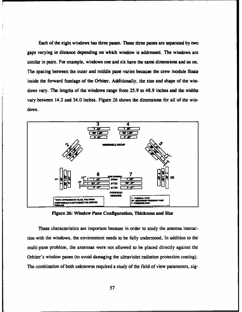
Each of the eight windows has three panes. These three panes are separated by two
gaps varying in distance depending on which window is addressed. The windows are
similar in pairs. For example, windows one and six have the same dimensions and so on.
The spacing between the outer and middle pane varies because the crew module floats
inside the forward fuselage of the Orbiter. Additionally, the size and shape of the win-
dows vary. The lengths of the windows range from 25.9 to 48.9 inches and the widths
vary between 14.2 and 34.0 inches. Figure 26 shows the dimensions for all of the win-
dows.
3 4Hhi 4r i I T _r I
IZ8
"t O-r-'-r-f--'--OMMo I p ..,--- I an .r :.
Figure 26: Window Pane Configuration, Thickness and Size
These characteristics are important because in order to study the antenna interac-
tion with the windows, the environment needs to be fully understood. In addition to the
multi-pane problem, the antennas were not allowed to be placed directly against the
Orbiter's window panes (to avoid damaging the ultraviolet radiation protection coating).
The combination of both unknowns required a study of the field of view parameters, sig-
57
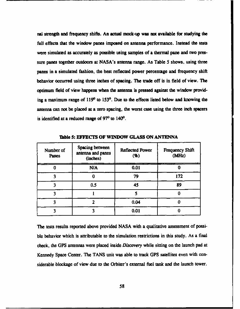
nal strength and frequency shifts. An actual mock-up was not available for studying the
full effects that the window panes imposed on antenna performance. Instead the tests
were simulated as accurately as possible using samples of a thermal pane and two pres-
sure panes together outdoors at NASA's antenna range. As Table 5 shows, using three
panes in a simulated fashion, the best reflected power percentage and frequency shift
behavior occurred using three inches of spacing. The trade off is in field of view. The
optimum field of view happens when the antenna is pressed against the window provid-
ing a maximum range of 119o to 1530. Due to the effects listed below and knowing the
antenna can not be placed at a zero spacing, the worst case using the three inch spacers
is identified at a reduced range of 970 to 140°.
Ikble 5: EFFECTS OF WINDOW GLASS ON ANTENNA
Number of Spacing between Reflected Power Frequency ShiftPam antenna and panes R d (MrHz)(inches)
0 N/A 0.01 0
3 0 79 172
3 0.5 45 89
3 1 5 0
3 2 0.04 0
3 3 0.01 0
The tests results reported above provided NASA with a qualitative assessment of possi-
ble behavior which is attributable to the simulation restrictions in this study. As a final
check, the GPS antennas were placed inside Discovery while sitting on the launch pad at
Kennedy Space Center. The TANS unit was able to track GPS satellites even with con-
siderable blockage of view due to the Orbiter's external fuel tank and the launch tower.
58

Unfortunately, position errors were difficult to characterize due to large multipath
effects from surrounding bodies. Although the three inch spacers gave higher signal lev-
els, STS-51 decided to use the one inch spacers for their flight in order to increase the
field of view.
An unsuccessful attempt to fly a similar version of this experiment aboard STS-56
demonstrated a "false-lock" phenomenon. This condition occurred when the antenna/
preamplifier units were placed near a PGSC. After thorough research, NASA discovered
that the Grid laptop computers were emitting an interfering signal at or near the GPS Li
frequency. It was also discovered that this interference was magnified by metal enclo-
sures, such as the Orbiter's crew cabin. An RF absorber was designed for this particular
reason, to counter these interferences inside the crew cabin. A maximum size for these
RF absorbers was derived from window viewing requirements. The only other option
available to minimize electromagnetic interference was by setting the receiver's signal
threshold above the PGSC's noise level. The following figure, Figure 27, shows that
although the signal threshold of 5 AMUs was set, the TANS receiver continued to lock
on and track the computers.
OWWI I No LWgl~ am TM..&4 sm "000"41 s
=__ 9777= _ z Jw___'_'-- I . ..--___ . ... ._____ -4---- --- l
FIgure 27: PGSC Interference Signal
59
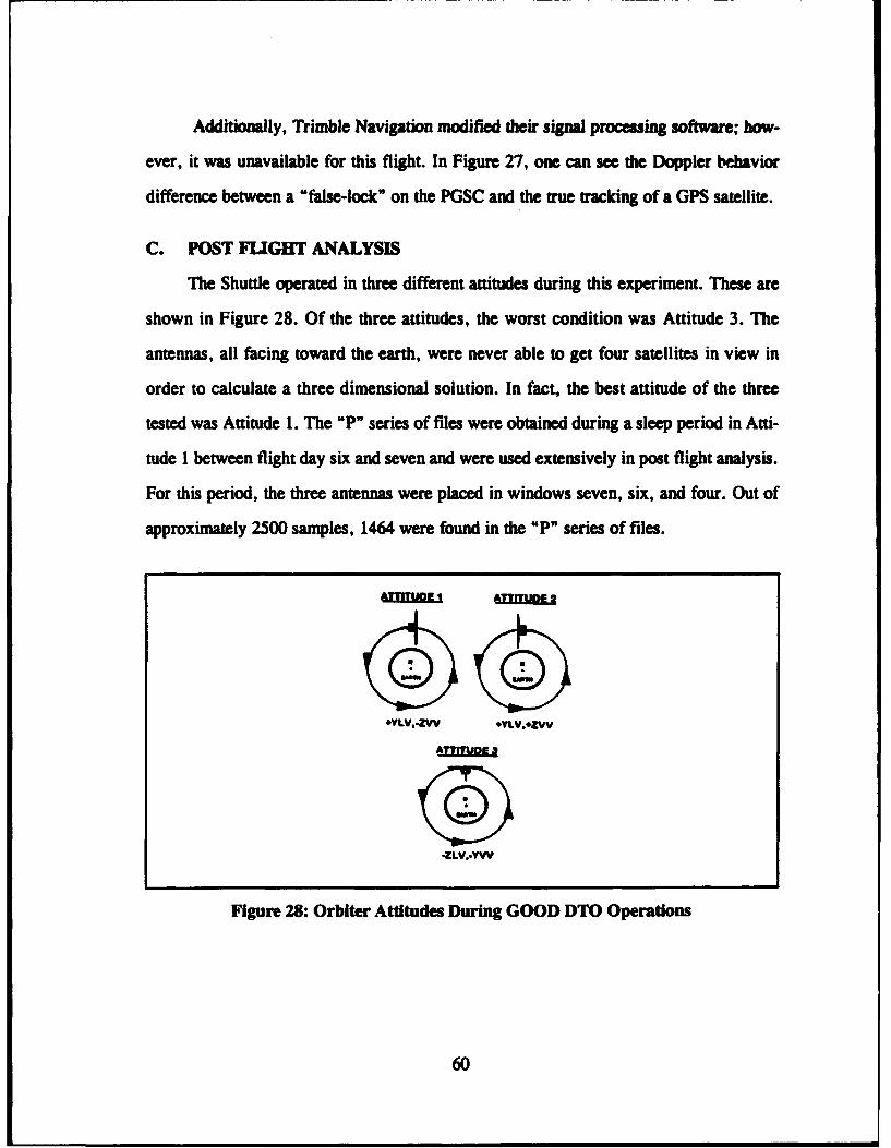
Additionally, Trimble Navigation modified their signal processing software; how-
ever, it was unavailable for this flight. In Figure 27, one can see the Doppler behavior
difference between a "false-lock" on the PGSC and the true tracking of a GPS satellite.
C. POST FLIGHT ANALYSIS
The Shuttle operated in three different attitudes during this experiment. These are
shown in Figure 28. Of the three attitudes, the worst condition was Attitude 3. The
antennas, all facing toward the earth, were never able to get four satellites in view in
order to calculate a three dimensional solution. In fact, the best attitude of the three
tested was Attitude 1. The "P" series of files were obtained during a sleep period in Atti-
tude I between flight day six and seven and were used extensively in post flight analysis.
For this period, the three antennas were placed in windows seven, six, and four. Out of
approximately 2500 samples, 1464 were found in the "P" series of files.
*YLV..ZVV +YLV.*ZVV
ZLV.-YVW
Figure 28: Orbiter Attitudes During GOOD DTO Operations
60
In conclusion, the attitude of the Orbiter provided a suboptimal environment for
viewing the GPS constellation given that the antennas were required to be inside the
crew cabin. Placing the antennas outside in the Orbiter's Payload Bay, for example,
would improve the performance of the receiver because the issues concerning foam
spacing and cockpit noise would disappear. However, the field of view and other poten-
tial errors would need to be characterized. Finally, the errors discussed in this chapter
were recognized by NASA and future follow-on experiments will be modified to mini-
mize these problems areas.
61
VI. CONCLUSIONS
A. FLIGHT HARDWARE
One of the chief aims of the GOOD DTO was to keep costs to a minimum. This
goal was readily achieved, but at the expense of some capabilities that might otherwise
have been available. Two specific improvements in flight hardware would greatly
enhance the performance of GPS aboard the Space Shuttle. Each of these improvements
would, however, have a significant cost associated with it.
The first suggested improvement is the use of space qualified equipment. This fea-
ture would permit components to be located outside the friendly environment of the crew
cabin, in the Shuttle's payload bay. This is particularly desirable in the case of the anten-
nas, whose in-cabin field of view is greatly restricted. Better visibility should enable four
satellites to be in view for a much higher percentage of time, resulting in more consistent
availability of the GPS state. A corresponding reduction in PDOP would also be
expected, correlating to improved GPS navigation accuracy.
The second suggestrA improvement is the use of a Precise Positioning Service
receiver. This is particularly desired because of the unsatisfactory velocity results
obtained by this experiment due to Selective Availability (SA) . The velocity accuracy of
the PPS is 0.2 meters per second. This is the order of magnitude of the desired accuracy
for velocity information. The velocity accuracy of the Standard Positioning Service is
classified, but errors observed during this experiment were on the order of 2 meters per
second. Velocity errors this large are unsuitable for use in navigation, as even small
velocity errors cause large position errors when used for propagating states. Use of a
Kalman Filter earlier in the receiver's logic would smooth both position and velocity to
an acceptable level. While a filtering scheme may succeed in reducing some of the error,
62
the only way to consistently achieve desired velocity accuracies is through use of a PPS
receiver.
B. FLIGHT SOFTWARE
The flight software functioned as it was designed, successfully recording data for
postflight analysis. The only desirable modification to the software would be the addition
of a relatively fast filtering algorithm, such as a version of the Kalman Filter designed to
smooth GPS state vector output. Again, incorporation of this feature would carry an
associated cost of further integration and testing.
C. FUTURE APPLICATIONS
Each of the suggested improvements to the GOOD DTO are already incorporated
as part of the design of the GPS navigation system being designed for the Shuttle.
(Kachmar, 1993, pp. 313-326). No plans exist to fly the GOOD DTO, as configured on
STS-51, again at a future date. However, portions of the experiment have been utilized
for two Shuttle missions since the September 1993 STS-51 flight, and STS-66 is sched-
uled to carry a portable GPS receiver, with antennas mounted in the payload bay, later
this year. The GOOD DTO has shown that good on orbit position accuracy can be
obtained using an inexpensive portable GPS receiver. The output of such a receiver can
be used by any application or experiment requiring precise timing or position informa-
tion.
63
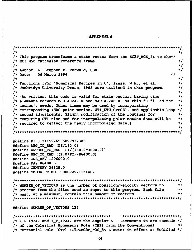
APPENDIX A
/ ********************************* ** */
/* This program transforms a state vector from the ECEF_WGS_84 to the*//* ECIMS0 cartesian reference frame.
/* Author: LT Stephen P. Rehwald, USN/* Date: 06 March 1994
/* Functions from "Numerical Recipes in C", Press, W.H., et al,/* Cambridge University Press, 1988 were utilized in this program.1* */* (As written, this code is valid for state vectors having time *//* elements between MJD 49247.0 and MJD 49248.0, as this fulfilled the *//* author's needs. Other times may be used by incorporating/* corresponding IERS polar motion, UTIUTCOFFSET, and applicable leap */7* second adjustments. Slight modification of the routines for/* computing UTI time and for interpolating polar motion data will be */I* required to reflect the newly incorporated data.)/* **************************************
#define PI 3.1415926535897932385#define DEG TO_RAD (PI/180.0)#define ARCSECTO RAD (PI/(180.0*3600.0))#define SECTORAD ((2.0*PI)/8640(.0)#define ONEREV 1296000.0#define DAY 86400.0#define CENTURY 36525.0#define OMEGAPRIME .000072921151467
/************************************************************************/*1* NUMBER OF VECTORS is the number of position/velocity vectors to/* process from the files used as input to this program. Each file/* must, at a minimum, contain this number of vectors./************************************************************************I*
#define NUMBEROFVECTORS 139
/* X_P_49247 and Y_P_49247 are the angular c. ,.acements in arc seconds *//* of the Celestial Ephemeris Pole (CEP) from the Conventional/* Terrestial Pole (CTP) (CTP=ECEFWGS_84 Z axis) in effect at Modified *1
64

/* Julian Date (MJD) 49247.0. Likewise, XP_49248 and YP_49248 are/* these values at MJD 49248.0. UTIUTC_49247 and UTIUTC_49248 are the *//* differences in seconds between the UTI and UTC timescales at MJD *//* 49247.0 and MJD 49248.0 respectively. Ex: UTI-UTIUTC_49247=UTC./* TAIUTCOFFSET is the integer difference in seconds between/* International Atomic Time (TAI) and UTC. Ex: TAI-TAI UTC OFFSET=UTC. *//* This difference is exact, and changes at not less than six month/* intervals through introduction of leap seconds. TDTTAIOFFSET is/* the set difference in seconds between Terrestrial Dynamical Time *//* (TDT) and TAI. Ex: TDT-TDTTAIOFFSET=TAI. Future predicted, and/* past observed values of xp, yp, & utiutc, as well as *//* TAIUTCOFFSET and TDTTAIOFFSET are published by the International *//* Earth Rotation Service (IERS) (in the U.S., by the National Earth *//* Orientation Service (NEOS)). The following were obtained by *//* directing an anonymous FTP into MAIA.USNO.NAVY.MIL to access the *//* SER7 directory./************************************************************************/*
#define X P_49247 -. 097#define YP _49247 .345#define UTI UTC 49247 .4570#define XP 49248 -. 097#define YP_49248 .347#define UTI UTC_49248 .4543#define TAI UTC OFFSET 28.0#define TDTTAIOFFSET 32.184
/* GPS UTC OFFSET is the inte• difference in seconds between GPS time *//* and Coordinated Universal (UTC). Ex: GPS-GPS UTCOFFSET=UTC./* For Standard Positioning Seivice (SPS), GPS time is accurate to *//* within 337 nanoseconds of UTC time after GPSUTCOFFSET is applied. *//* GPSWEEKNUMBER is the number of weeks elapsed since 06 JAN 80./* GPSUTCOFFSET and GPSWEEKNUMBER are transmitted in NAY-messages *//* from GPS Satellite Vehicles (SVs). JDGPSWEEK_0 is the Julian Date *//* at Oh 06 JAN 80 in UTC. */
#define GPS UTC OFFSET 9.0#define GPSWEEKNUMBER 714.0#define JDGPSWEEK_0 2444244.5
/*************************************************************************/* JD_00 JAN 93 is the Julian Date at Oh 00 JAN 93 in UTC. JD J2000 is *//* the Julian Date at Standard Epoch J2000.0 in Barycentric Dynamical *//* Time (TDB).
65
#define JD_00_JAN_93 2448987.5#define JDJ2000 2451545.0
#include <bcd.h>#include <math.h>#include <stdio.h>#include <stdlib.h>
void nerror(char*);
FILE *j,*k;int n,o,i;long doublea_i[106 (5],5s_i[106H (2],c_i[106] [2],an[(4] 5],s_n[4] [2],c_n(4] [2];long double m_0[3H 3],t_0[NUMBEROFVECTORS] [6]';long double v_0 (NUMBEROFVECTORS] [6] ,v_1 [NUMBEROFVECTORS] [6] ;
/* nerror is Numerical Recipes standard error handler/* *
void nerror (char errortext [()(fprintf (stderr, "Numerical Recipes run-time error... \n");fprintf (stderr, "%s\n", errortext);fprintf(stderr,"...now exiting to system... \n");_exit (1) ;
/.**
/* a_i]([],s_i[](], and c_i[][] are the IAU 1980 Nutation series/* multipliers and coefficients (Table 3.222.1, Explanatory Supplement *//* to the Astronomical Almanac, 1992). *//* an( n [],s_n[] [1, and c_n(] [] are multipliers and coefficients for/* corrections to the IAU 1980 Nutation series (Table 3.224.1, *//* Explanatory Supplement to the Astronomical Alamanac, 1992)./* m_0[] (] is the transformation matrix from B1950.0 to J2000.0 a.k.a. *//* DE118/LE62 to DE200/LE200 (E.M. Standish, Astronomy and Astrophysics *//* 114, pp. 297-302, 1982)./* t 0(i] [0] is the time element of the ith state vector in seconds *//* since the beginning of the week (GPS time). t_0[i] [0]==t_0[i] [1]./* t_0[i] [2] is the time element of the ith state vector in hours/* since the beginning of the year (UTC) (Consistent with the Orbiter */
66
* reference trajectory state vectors supplied by NASA JSC). *//* t_0(i) (31 is the Julian Date of the ith state vector in TDB. *//* t_0[i] [41 is the Julian Date at Oh on the day of interest in UTI. *//* t 0(i) (5) is the time element of the ith state vector in seconds* since the beginning of the day (UTC).
/* v_0(i) [01, v_0[(i) Ell, and v 0(i][21 are the X, Y, and Z Cartesian/* position coordinates, respectively, of the ith state vector in the */* ECEFWGS_84 reference frame.* v_0(i1 (3), v_0(iI (41, and v 0(i) (5] are the XDOT, YDOT, and Z_DOT */
/* cartesian velocity coordinates, respectively, of the ith state/* vector in the ECEFWGS_84 reference frame. *//* v_1[i) [01, v_l(il [11, and v_l(il (21 are the X, Y, and Z cartesian *//* position coordinates, respectively, of the ith state vector in the *//* ECI M50 reference frame./* v l(ii (2], vl~il (41, and vl[i] [51 are the XDOT, YDOT, and ZDOT *//* cartesian velocity coordinates, respectively, of the ith state */1* vector in the ECI M50 reference frame. */I*
* ECEF WGS 84 coordinates/GPS time are read from ASCII position and. velocity data files, created by the TANSPOST program, which extracts */. desired data from the binary data files created by the TANSIO. program on STS-51. Transformed ECI_M50 coordinates/UTC are written */. to an ASCII data file.. FILE SPECIFICATIONS: -ECEF WGS_84 Position File Name = statep.001. -ECEF _WGS _84 Velocity File Name = statev.001 */*/. -ECI M50 State Vector File Name = stateout.001 */*/. -Data appearing on the same line in both input */J* files must correspond to the same time */
*i. element. *1*/. -The number of vectors in the input files must */. be equal to or greater than the number*/. appearing in the #define NUMBEROFVECTORS */I/. preprocessor statement. */
I, *
. From TANS packet 41:
. GPS UTC OFFSET = 9 seconds throughout the mission.
. GPSWEEKNUMBER = 714 starting 12 SEP 94
. GPS WEEK NUMBER = 715 starting 19 SEP 94 */* The correct numbers must appear in the #define preprocessor */* statements.
'*
* Coordinate conversion methodology: */* ECIM50 position = [abcpm_0]transpose * ECEFWGS_84 position */"* ECIM50 velocity = (abdotcpmo0transpose * ECEFWGS_84 position + */"* (abcpmOltranspose * ECEFWGS_84 velocity */* a, b, bdot, c, p, and m_0 are rotation matrices for polar motion,
67
/* Earth rotation, rate of change of Earth rotation matrix, astronomic *f/* nutation, general precession, and standard epoch conversion, *//* respectively, a through p are time varying 3x3 matrices, though only *//* the rate of change of b is significant. m_0 is a constant 3x3 *//* matrix.
void main(void){long double longest=0.0;
// Initialize Nutation series a_i[] (I s_i[] (] c_i[] [I a_n(i [I sn[(] [I c_n(] I]*for (n=0 ;n<106 ;n++){
for(o=0;o<5;o++){a i[nl[o]=0.0;}
for (o=0 ;o<2 ;o++){s-i(n] (o1=0.0;c i[nl[o]=0.0;}
}for (n=0 ;n<4 ;n++){
for(o=O;o0<5;o++)
a n[nJ [o(=0.0;}for(o=0;o<2;o++){
Sn[nnl[ol=0.0;c n(n] [o]=0.0;
a i[0] [41=1.0; a i[1] [41=2.0; a_i[2] [0]=-2.0; a_i[21 [21=2.0; a_i[21 [41=1.0;a i[31 [01=2.0; a_i[31 [2]=-2.0; a_i[4] [0]=-2.0; a_i[4] [21=2.0;a_i[4] [41=2.0; a_i[5] [01=1.0; ai[5] 1[]=-1.0; a_i[5] [31=-1.0;a_i(6] [1]=-2.0; a_i[6] [2]=2.0; a_i[6] [3]=-2.0; a_i[61 [4]=1.0;a_i(7] [01=2.0; a_i[71 [21=-2.0; a_i[7] [41=1.0; a_i[8] [2]=2.0;a_i(8] [31=-2.0; a_i(8] [41=2.0; a_i[9] [(]=1.0; a_i[10] [11=1 0;a_i(101 (21=2.0; a_i[10] [3]=-2.0; a_i[101 [4]=2.0; a i[l1] [1]=-1.0;a_i[11] [2]=2.0; ai(111 [31=-2.0; a i[11] (41=2.0; a_i(121 [21=2.0;a i[121 [3]=-2.0; a_i[121 [41=1.0; ai[131 [01=2.0; a-i[13] [31=-2.0;a_i[141 [21=2.0; a_i[141 [3]=-2.0; ai[151 [11=2.0; a-i[161 [1]=1.0;
68
a_i(16] (41=1.0; a_i[17] (11=2.0; a_i[17] (21=2.0; a i(171 [31=-2.0;a i[17] [41=2.0; a_i(18] [11--i.0; a_i[18] [41=1.0; a_i[191 [0].-2.0;a_i[19] (31=2.0; a_i(191 [41=1.0; a_i[201 (11=-I.0; ai[201 [21=2.0;a_i(201 [31]-2.0; a._i[201 [41=1.0; a._i[211 [01-2.0; ai[211 [31=-2.0;a i(211 [41=1.0; a_i(22] [11=1.0; a_i[221 [21=2.0; a_i[221 [31=-2.0;a_i[22] [41=1.0; a_i(23] (01=1.0; a_i[23] [31=-1.0; ai[24][0]=2.0;a_i[241 [1]=1.0; a_i(24] [31=-2.0; a_i[25] [2]=-2.0; a_i[25] [31=2.0;a_i[251 [41=1.0; a_i(26] [11=1.0; a_i[261 [2]=-2.0; a_i[261 (31=2.0;a_i[271 (111-.0; a_i[27] [41=2.0; a_i[281 [0]=-1.0; a_i[281 [31=1.0;a i[28] [41=1.0; a_i[291 [11=1.0; a_i[29] (2]=2.0; a i(29] [3]=-2.0;a_i[30] [21=2.0; a_i[30] (41=2.0; a i[311 [01=1.0; a_i[321 (21=2.0;a_i[321 [41=1.0; a_i(331 [01=1.0; a_i[331 [21=2.0; a_i(331 (41=2.0;a_i(34] [01=1.0; a_i[34] [31s-2.0; a_i[35] [01=-1.0; a_i[35] [21=2.0;a_i(35] (41=2.0; a_i[36] (31=2.0; a_i[37] [01=1.0; a_i[371 [41=1.0;a_i[38] [0]=-1.0; a_i[381 [41=1.0; a_i[391 [01=-1.0; a_i(39] [21=2.0;a_i(39] (31=2.0; a_i[39] [41=2.0; a_i[40] [01=1.0; a i[40] [21=2.0;a_i[40] [41=1.0; a_i[41] (21=2.0; a_i[41] [31=2.0; a_i[41] [41=2.0;a_i[421 [01=2.0; a_i[43] [01=1.0; a_i[431 [21=2.0; a_i[43] [31=-2.0;a i[43] [41=2.0; a_i(44] [01=2.0; a_i(441 [21=2.0; a_i(441 (41 =2.0;a_i[45] [21=2.0; a_i[461 [01=-1.0; a_i(46] (21=2.0; a_i(461 [41=1.0;a_i[47] [01=-1.0; a_i(47] [31=2.0; a__i[471 [41=1.0; a i[48] [01=1.0;a_i[481 [31=-2.0; a_i(48] [41=1.0; ai[49] [01=-1.0; a i[491 [21=2.0;a_i[49J (31=2.0; a_i[49] [41=1.0; ai[50J (01-i.0; ai[50 ([I1=1.0;a_i[S0] [31=-2.0; a_i[51] [11=1.0; a_i[51] (21=2.0; a_i(511 (41=2.0;a_i[52] [1]=-1.0; a_i[521 (21=2.0; a_i[52] [41=2.0; a_i[53] [01=1.0;a_i(53] [21=2.0; a_i[53] [31=2.0; a_i(53] [41=2.0; a i[541 [01=1.0;a_i[54] [31=2.0; a_i[55] [01=2.0; a_i[55] [21=2.0; a--i[551 [3]=-2.0;a_i[55] [41=2.0; a_i[56] [31=2.0; a_i[561 [41=1.0; ai[571 [2]=2.0;a_i[57] [31=2.0; a_i[57] [41=1.0; a_i[58] [01=1.0; a i[581 [21=2.0;ai(58] [31=-2.0; a_i[58] [4121.0; a_i[59] [31=-2.0;-a_i[591 [41=1.0;a_i[60] [01=1.0; a_i[601 [1]=-1.0; a_i[61] [01=2.0; a_i[61] [21=2.0;a_il[61 [41=1.0; a_i[621 [11=1.0; a_i[62] [31=-2.0; a i[631 [01=1.0;a_i[631 [2]=-2.0; a_i[641 [31=1.0; a_i[65] [01=1.0; a-i[651 [11=1.0;a_i[66] [01=1.0; a_i[66] [21=2.0; a_i[67] [01=1.0; ai1[671 [11=-1.0;a_i[67] [21=2.0; a_i(67] [41=2.0; a_i[68] [01=-1.0; a i[681 [11=-1.0;a_i[681 [21=2.0; a_i[68] [31=2.0; a_i[68] [41=2.0; a_i[691 [01=-2.0;a_i[69] [41=1.0; a_i[70 ([01=3.0; a_i[70] [21=2.0; a i[701 [41=2.0;a_i[71] [11=-1.0; a_i[71] [21=2.0; a_i[71] [3]=2.0; a_i(711 (41=2.0;a_i[72] [01=1.0; a_i[721 [11=1.0; a_i[72] [21=2.0; a i[72] (41=2.0;a_i[73] (0]=-1.0; a_i[73] (21=2.0; a_i[73] [3]=-2.0; a_i[73] [41=1.0;a_i[74] [01=2.0; a_i[74] [41=1.0; a_i[75] [01=1.0; a_i[75] [41=2.0;a_i[761 (01=3.0; a_i[77] (21=2.0; ai[77] [31=1.0; a_i[77] [41=2.0;a_i(78] [0]=-1.0; a_i[78] [41=2.0; a_i[79] [0]=1.0; a i[79] [3]=-4.0;a_i[80] [0]=-2.0; a_i[80] [21=2.0; a_i[80] [31=2.0; a_i[80] [41=2.0;a_i[81] [0]=-1.0; a_i[81] [21=2.0; a_i[81] [31=4.0; a i[811 [41=2.0;a i[82] [01=2.0; a_i[82] [31=-4.0; a_i[831 [01=1.0; a_i(831 [11=1.0;
69
a_i (831 (21-=2. 0; a,_i([831 [31]-2. 0; ai (831 (41=-2. 0; aý_i (84] (0 1. 0;a_ i(841 [ 21 =2. 0; aý_i([841 [31 =2. 0; aý_i[(841 [41 -1. 0; aý_i[1851 (01 -2. 0;a- [851 [21=-2. 0; ai (851 [31 =4. 0; ai([851 (4]=-2. 0; a-i([861 (01 -l. 0;ai i[861 [2)1=4. 0; a_i [861 [41 =2. 0; a-i [871 [0)=1. 0; a-i [87] [11=-l. 0;a-i (871 [3) =-2. 0; aý_i[(881 [0)1=2. 0; a_i([88] (2)1=2. 0; aý_i (881 (3) -2. 0;ai i(881 (41=-1. 0; a_i (891 (01 -2. 0; a_i (89] [21=-2. 0; a-i (891 (31 =2. 0;a-i([891 [4)1=2. 0; a,_i (9 01 [01 -1. 0; aý_i[(901 [31=.2. 0; aý_i [90] [41.1. 0;a-i([911 (21 =4. 0; a-i (9 11 (31--2. 0; a-i([9 11 [41 =2. 0; a-i([921 [01 3. 0;a-i [921([21 =2. 0; aki [ 921[3]=--2. 0; a-i [921 [41=2. 0; a,.i [93] (0) 1.0;ai [(931 [21=-2. 0; a,_i (931 [3)1-2.0; aý-i[941 (11 =1. 0; a-i [941 [21 =2. 0;ai 1(941 (41=-1. 0; ai [951[01=-1.0; ak_i([951[(11 =-l.0; a,_i(951([31 =2. 0;a-i [951 (41 =1. 0; a_1([9 61 [21=--2.0; a_i([96] (411i. 0; aý_1(971 [21 =2. 0;ai 1(971 (31--1.0; ak_i[97] (41=2.0; a_i[9 81 (11=1.0; a,_1(98] (31=2.0;a-i[991 [01 =1.0; a_1([991 [21 -- 2.0; a_1 9 9] 13]=-2.0; a_1i(100] [1]=-1.0;a_1([1001 (21 =2. 0; aý_1(1001 (41 =1. 0; a,_i[(101] [01 =1. 0; aý_1(1011 (11 =1. 0;a_1 (1011 (31 -- 2. 0; a_1( 1011 [41-1i.0; a_1i(1021 [011i. 0; aki [1021 (21 =-2. 0;a_1([1021 (31 =2. 0; aý_1(1031 (01=.2. 0; a_1([103] [31 =2. 0; aý_i (104] (21 =2. 0;a-i (1041 [31 =4. 0; aý_i[(104] [41 =2. 0; ak_1(1051 [l=1. 0; a_1([1051 (31=-1.0;s_[10][0]=-171996.0; B_1(0] [1]=-174.2; s_i(11 (01=2062.0; s_i1(1][11=.2;s i(21 [01=46.0; 5_i(3] (01=11.0; s_i(41 (0]=-3.0; s_i(51 (0]=-3.0;s-i(61 (0]=-2.0; s_1(7] [01=1.0; s_1[S(81(0=-13187.0; s_1(81 [11=-1.6;s_1(91 (01=1426.0; s_1(9] (1]=-3.4; S_i[101 (01=-517.0; s_i(101 [11=1.2;s-i(11](0]=217; s_i[111[11=-.5; s_i(12](0]=129.0; s-i(121[11=.1;s_1(131(01=48.0; s-i(141[0]=-22.0; s_i(151(01=17.0; s_i(151(1]=-.1;S i(161 (01=-15.0; s_i[17] (01=-16.0; s_1(171 [11=.1; s_i[181 [0] -- 12.0;s-i(191 [01=-6.0; s_i[201 [01=-5.0; s_1(21] (01=4.0; s_i(221 [01=4.0;s_1(231 (0]=-4.0; s_1(24] (01=1.0; s_1(251 (01=1.0; s_1(261 (01=-1.0;a-i(271 (01=1.0; s_1(28] (01=1.0; a_i(291 (01=-1.0; si(301 (0J=-2274.0;s_1(301 (11=-.2; a_1(311 [01=712.0; s_i(311 (11=.1; s-i(321 (01=-386.0;s-i(321 (1]-.4; s_1(331 (01=-301.0; s_1(341 (0]=-158.0; s_1(35] [01=123.0;B_1(361 (01=63.0; s-i[37] [01=63.0; s_1(37] [11=.1; s~i(381 (0]=-58.0;s_1(381 [1]=-.1; 5_1(391 (01=-59.0; s_i(40] (0]=-51.0; s_i(411 (0]=-38.0;s_1(421(01=29.0; S-i(43][01=29.0; s_i(441(0]=-31.0; s_1(451(01=26.0;s_1(461 (01=21.0; S_1(471 (01=16.0; a_i(481 [01=-13.0; s_1(491 (0]-10.0;s_1(501 (0]=-7.0; s_i[51] (01=7.0; a_1(52] (01=-7.0; s_1(531 (0]=-8.0;s_1(541 [01=6.0; S_1(551 (01=6.0; s_1(561 (01=-6.0; a_1(571 [01 =-7.0;s_1(58] (01=6.0; s_1(591(01=-5.0; s_1(601 (01=5.0; s-i(611 (0]=-5.0;s i(62] (01=-4.0; s-i(63] (01=4.0; s_1(641 (01=-4.0; s-i(65] (01=-3.0;s_1(661 (01=3.0; Si(67] [01=-3.0; s_1(681 (01=-3.0; s_1(691 (0]=-2.0;s-i[70] (0]=-3.0; S_i(711 (01=-3.0; s-i(72] (01=2.0; S-i(73] (01=-2.0;s_1(74] (01=2.0; s_1(75] (0]=-2.0; s-i[76] [01=2.0; S_1(771 (01=2.0;s_1(78] (01=1.0; S_1(79](01=-1.0; s-i(801 (01=1.0; s-i(811 [0]=-2.0;s-i(821 (01=-1.0; s_i(831 (01=1.0; s_1(841 (01=-1.0; s_i(851 (0]=-1.0;s 1(861 (01=1.0; s i[871 (01=1.0; s_i(881 (01=1.0; s 1(891 (0]=-1.0;s_1(901 (01=-1.0; s_i(91] (01-1.0; s_1(92] (01=1.0; s_1(931 (01=-1.0;s_1(941 (01=1.0; s 1(951 (01=1.0; s_i(961 [01=-1.0; a_1(97] (0]=-1.0;
70

_ -i[981 (01=-1.0; S-i(991 (01-1.0; S-i[1001 [01--1.0; S -i(1011 [01=-1.0;s_-i(1021[01=-1.0; S_i(1031(O]=1.0; S -i(1041[01=-1.0; S-i(105H[0]=1.0;c_-iC(l(01=92025.0; C i(01 [13=8.9; C-i(1] (01=-895.0; C_i(11 [1]=.5;_ -i[21[(01=-24.0; C-i(41 (01-1.0; c-i(61 (01=1.0; c-i(81 (01=5736.0;_ -i(81[(11=-3.1; c-i(91 (01=54.0; c -i[91 [11=- .1; c_i(101 (01=224.0;
c -i[10] [1]=-.6; c -i[11] [0]=-95.0; C_i(111 (1]=.3; c_i(121 (0]=-70.0;c i(131[(01=1.0; c -i(16] [01=9.0; c-i(17] (01=7.0; C_i[181 (01=6.0;
_ i[19] (01=3.0; c -i[20] (01=3.0; C_i(211 (0]=-2.0; C-i(221 (01=-2.0;c i(30] (01=977.0; C_i(301 (11=-.5; c -i[311 (01=-7.0; C-i(321 (0]=200.0;c i(33] (01=129.0; c-i(331 (1]=-.1; C-i(341 [0]=-1.0; C-i[35] (01=-53.O;c i[361[(01 =-2.0; C_i&37] [01=-33.0; C_i[381 (01=32.0; C-i(391 [0] =26.0;c i(40] (01=27.0; C_i(411 (01=16.0; c_i[42] (01=-1.0; c -i[431[(01=-12.0;c i(44][(01=13.0; c-i(45] (01=-1.0; c -i[461[(01=-10.0; C-i(47] (01=-8.0;c i[48] (01=7.0; c-i(491 (01=5.0; c-i[511 (01=-3.0; C-i[52] (01=3.0;c-i(531 (01=3.0; C_i(55] (01=-3.0; C_i(56] (01=3.0; C-i(571 (01=3.0;c i(581[(0]=-3.0; C_i[591 (01=3.0; c i[611 [01=3.0; C_i(671 (01=1.0;c i(68] (01=1.0; c-i(691 (01=1.0; c-i(701 (01=1.0; C_i[711 (01=1.0;c i[72] (0]=-1.0; C_i(73] (01=1.0; C_i(741 (0]=-1.0; C_i(75] (01=1.0;c-i(77] [0]=-1.0; C_i[78] [01=-1.0; C_i(801 (0]=-1.0; C_i(811 (01=1.0;c-i(83] (01=-1.0; c-i(841 (01=1.0; C-i(851 (01=1.0; C_i(88] (01=-1.0;a-n(01 (41=1.0; a_n(11 (11=1.0; a,_n(2] [21-2.0; a_n(2] 131=-2.0; a,_n(21 (41=2.0;a-n(3] [21=2.0; a_n(3] (41 =2.0;s -n[01[(01=-725.0; s-n(01 (11=224.0; s-nill (01=523.0; s-n(1] (11=-24.0;s -n[21[(01=102.0; s-n(21 (11=-47.0; s-n(31 (0]=-81.0;c-n(01 (01=417.0; c-n(01 (11=213.0; c_n(11 (01=61.0; c-n(11 [1] =208.0;c n[2] [0]=-118.0; c n(21[(11=-41.0; c n(31[(11 =32.0;
IIInitialize the DE118/L362 to DE200/LE-200 transformation matrix*************m_0(0][01=.9999256791774783; mr_0(1[11 J=-.0111815116768724;m_0(0](2] =-.0048590038154553; m_0(11[(0]=.0111815116959975;m_0(1]][11=.9999374845751042; m_0(11](21 =-.0000271625775175;m_0(2][0]=.004859003771445; mr_0(2]1(1]=-.000027170449221;m_0(2]1[2]=.9999881946023742;
IIRead ECEFWGS_84 state vectors from external filesif((j=fopen("'statep.001","r"l))==NULL)
fclose(j);nerror("lunable to open statep.001 in maino");
if( (k=fopen("'statev.001", "r") )==NULL)
fclose (k);nerror("lunable to open statev.001 in main()");
for(i=0;i<cNUMBEROFVECTORS;i++)
f scanf (j, "%-Lf ILf %Lf %Lf \n", &t_0 (ii (01 , &v_0 [ii (01 , &vý_0 [il [11
71
&vý_O (i][2])fscanf(k,"%Lf %Lf VLf %Lf\n",&t~o[i] (l],&v O[i] [3],&v_3[i] [4],
&v.O ci] (51) ;tO~i] [O]*=.lOO00O0.O; V_0[j] []*=1000000.O; v_-O~i] (l]*=lOOOOO.O;
v_0(i] (2] *1000000.0;t_0 (i] [l]*=lOOO.O; vý_O~i] [3]*=lOO.O; vO[i] [4]*=lOOO.O;
V0(i) (5] *1000 O*t_0(i) [o]+m522009.O; t_O[i] [1] +522009.0;if (i<5)
printf("*Lf %Lf\n",t_0(i) (O],t_O(i] (1]);
Iif(tO[i][0]!=tO~i](l])
nerror(otime element mismatch in maino");
if (f close (j) ==EOF)
nerror("unable to close statep.00l in maino");
if (f close (k) ==EOF)
nerror("lunable to close statev.O0l in maino");
IIMain loop to calculate time, rotation matrices, and transformations********for(i=0;i<NUMBEROFVECTORS;i++)
bcd tdt;long double g, integer, fraction;long double t, zeta, z, theta, p(3] (3]1long double l,l...prime,f,d,omega,epsilon-bar, epsilon,c[3] (3];long double uti-utc-interpolated, delta~psi= .0, delta epsilon=0 .0;long double t-u,hO,delta-h,omega _star,lambda,b(3] (3],b-dot(3] (3];long double xp interpolated,y~p interpolated,a(3] (3];long double pm_ 0(3] [(3] , cpmO 3] ( 3] , bcpmRO(3 [ 3]3 , b-dot cpmO( 3] (3];long double abcpmr_0(3] (3],ab dotcpmiO[3] (31;long double abcpmR_0_transpose(3] [3] ,ab dotcpmRO transpose(3] (3];
iiConvert time (t_-Ofi] (0] & t_0(i) [1]) to U!FC/TDB/IJT1 (t_-0[i) (2] - t_0(i) (5])IICompute UTC time in hours since the beginning of the year***************t_0(i) (2]=((t_0(i] (0]/DAY)+(GPSWEEKNTJMBER*7.0)+JDGPSWEEK_0-
(GPSUTCOFFSET/DAY)-JD_00_JAN_93)*24.0;IICompute Julian Date in TDT time rounded to two decimal places***********tdt=bcd(((t_0(i] [0]/DAY)+(GPsWEEKNUMBER*7.0)+JDGPSWEEK_0-
(GPS_-UTC_-OFFSET/DAY) +(TAIUTCOFFSET/DAY) +(TDTTAIOFFSET/DAY)) ,2);1/Compute mean anomaly of the Earth in itsobi*************
72
g=357.53+(.9856O03*(rea1(tdt)-JDIJ2000));I!Compute Julian Date in TDBtie********************tOfi] [3]=(tO-i 0[O][/DAY)+(GPSWEEK_-NUMBER*7.0)+JDGPSWEEK_0-
(GPS_-UTC_-OFFSET/DAY)+(TAIUTCOFFSET/DAY)+(TDTTAIOFFSET!DAY)+(((.00l658*sinl(g*DEGTORAD))+(.000014*sinl(2.0*g*DEGTORAD)))/DAY);
IICompute Julian Date in UT1r ie********************if(((t_0(Oi] [0]/DAY)+(GPSWEEKNUMBER*7.0)+JDGPSWEEK 0-
(GPSUTCOFFSET!DAY) -2400000.5) c49248.0)
tOti] [4]=(t_0[i] [0]/DAY)+(GPSWEEKNUMBER*7.0)+JDGPSWEEK_0-IGPSUTCOFFSET/DAY)+(UTlUTC_49247/DAY);
if(((t_0(i] [0]l/DAY)+(GPSWEEKNUMBER*7.0)+JDGPSWEEK 0-(GPSUTCOFFSET!
DAY) -2400000.5) >=49248.0)
t_0(i] [4]=(t_0[i] (0]/DAY)+(GPSWEEKNUMBER*7.0)+JDGPSWEEK_0-(GPSUTCOFFSET/DAY)+(UTlUTC_49248/DAY);
II Compute Julian Date in UTi time at the beginning of the day*************fraction=modfl (t_0 i[i(4] ,&integer);if (fraction< .5)
t_0[i] [4]=integer- .5;
if (fraction>.5)
t_0(i] [4]=integer+.5;
IICompute UTJC time in seconds since the beginning of the day**************fraction=modfl C C t_0[i] [0]-GPS *"COFFSET) /DAY) ,&integer);t_-0[i] [5]=(t_0[i] (0]-GPSUTCOFz11)ET)-(integer*DAY);
IICalculate General Precession Rotation Matrix p([] []*************
//Calculate number of centuries of TDB elapsed since J2000.0**************t=(t_-0 (ii[3] -JDJ2000) /CENTURY;
IICalculate Accumulated Precession Angles Adopted by IAU 1976*************zeta=((2306.2181*t)+(.30188*t*t)+(.017998*t*t*t))*ARCSECTORAD;z=((2306.2181*t)+(l.09468*t*t)+(.018203*t*t*t))*ARCSECTORAD;theta=((2004.3l09*t)-(.42665*t*t)-(.041833*t*t*t))*ARCSECTORAD;p (0](0 = (cosi (z) *cosl (theta) *cosl (zeta)) -(sinl (z) *sinl (zeta)) ;
p[0] [2] =-cosl(z) *sinl (theta);p~l] [0]=(sinl(z)*cosl(theta)*cosl(zeta))+(cosl(z)*sinl(zeta));
73
IICalculate Astronomical Nutation. Rotation Matrix c U(] [***********IICalculate IAU 1980 Nutation set of Fundamental Arguments****************l=(485866,.733+(((1325.o*ONE REV) +715922.633)*t)+(31.31*t*t)+(.064*t*t*t))*ARCSECTORAD;
lyprime=(1287099.804+( ((99.0*ONEREV) +1292581.244)*t) -(.577*t*t) -(.0l2*t*t*t))*ARCSEC_-TO_-RAD;
f=(335778.877+( ((1342.0*ONEREV) +295263.137) *t) -(l3.2S7*t*t)+(.0ll*t*t*t))*ARCSECTORAD;
d=(1072261.307+( ((1236.o*ONEREV) +1105601.328)*t) -(6. 891*t*t) +( .019*t~t*
t))*ARCSECTORAD;omega=(450160.28-( ( (.O*ONEREV) +482890.539) *t)+(7.455*t*t)+(.008*t*t*
t))*ARCSECTORAD,1/Calculate Mean obliquity of the Elpi****************epsilon -bar=(84381.448-(46.8l5*t) -(.00O59*t*t)+(.O018l3*t*t*t) )*
ARCSECTO_-R.AD;IICalculate Angle of Nutation in Longitude********************************for (n=0 ;n<106;n++)
long double delta~psi_i;delta~psi~i=(s-i In] [O]+ (s-i In] [1lJ*t) )*sinl ((a-i In] (01J*l)+ (a-i In] (11*
lprime) +(a Ti (n] (2] *f) +(a_i [n] (3] *d) +(a_i. (i] [4] *omega));delta~psi+=(delta~psi_i*.000l*ARCSECTORAD);
IICalculate and apply Correction to Angle of Nutation in Longitude********for (n=0 ;n<4 ;n++)
long double delta~psi_c;deltajpsi~c=(s-n[n] [0]*sinl((aý_n[n] (0]*l)+(a-n~n] [l]*l~prime)+
(a-n~n] [2]*f)+(a-n[n] [3] *d)+(a-n[nI [4] *omega)))+
(c-n[n] [0]*cosl((a_n[n] [0]*l)+(a-n[n] (l]*lprime)+
(a-n~n] [2]*f)+(a-n~n] [3]*d)+(a-n[n] [4]*omega)));delta...psi+=(delta...psi_c*.0000l*ARCSECTORAD);
IICalculate Angle of Nutation in Obliquity********************************for (n=0 ;n<106 ;n++)
long double delta -epsilon Ti;delta epsilon-i=(C-i[n] [0]+(c-i[n] [1]*t))*cosl((a-i[n] [0]*l)+
74
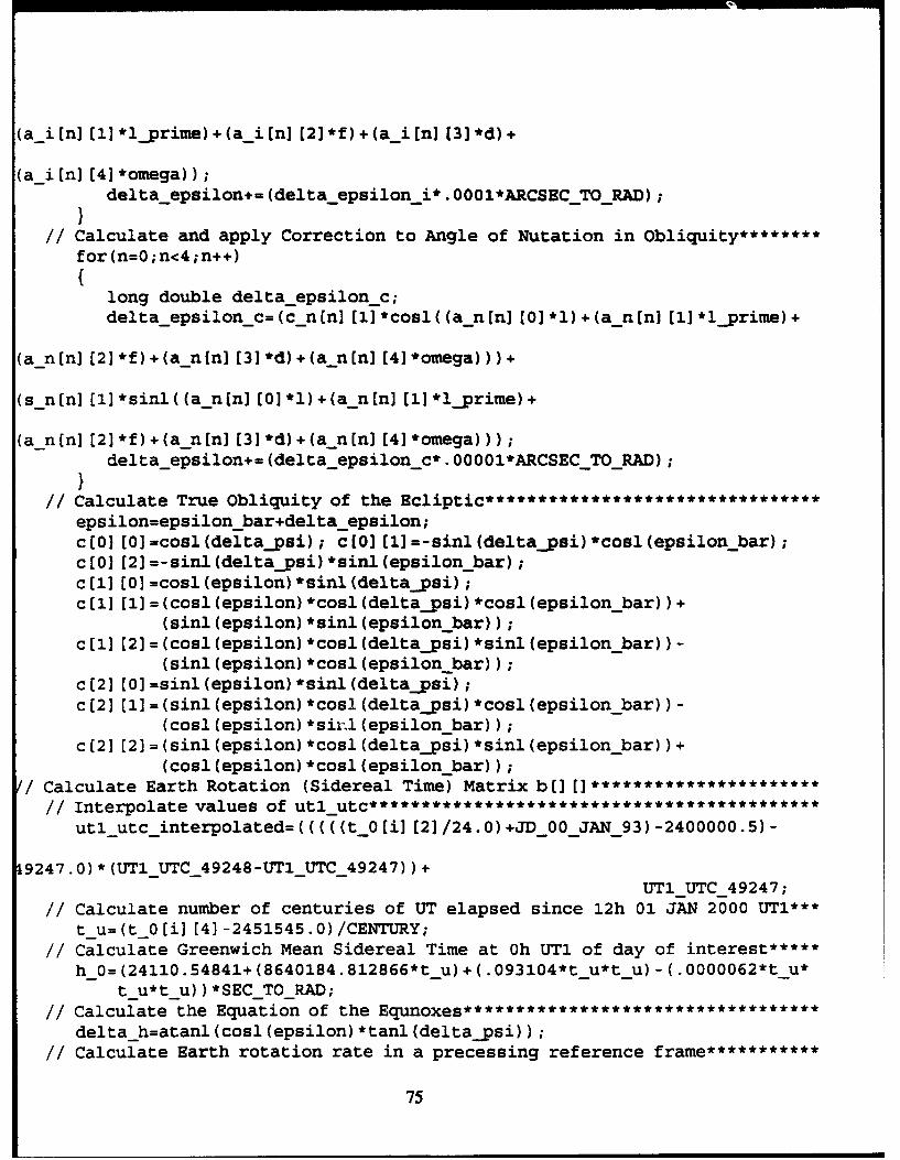
(a-i (n] (l] *1.prime) +(a-i [n] [2] *f) +(a-i [n] (31 *d) +
(a i [nI [4]*omega));delta epsilon+- (delta-epsilon i*.OO0l*ARCSECTORAD);
IICalculate and apply Correction to Angle of Nutation in Obliquity********f or (n=O ;n<4 ;n++)
long double delta epsilonc;delta epsilon-c=(c-n~n] (1]*cosl((a-n~nJ (0]*l)+(a-n~nJ [1] *lprime)+
(a-nfn] (2]*f)+(a-n[nJ [3]*d)+(a-n~n][4]*omega)))+
(s-n[n] [l]*sinl((a-n~n] (O]*l)+(a-n[n] [l]*lprime)+
(a-n(n] [2]*f)+(a-n~n] (3]*d)+(a-n~n] [4]*omega)));delta epsilon+= (delta-epsilon c*.00001*ARCSECTOR.AD);
IICalculate True Obliquity of the Elpi****************epsilon=epsilon-bar+delta -epsilon;c(O] [O]=cosl(delta-psi); cLO (il]=-sinl(delta-psi)*cosl(epsilon-bar);c[O] [2] =-sinl (delta-psi) *sinl (epsilon-bar);c [11[0] =cosl (epsilon) *sinl (delta-psi);c[l] [1] =(cosl(epsilon)*cosl(delta-psi)*cosl(epsilon-bar) )+
(sinl (epsilon) *sinl (epsilon -bar));c[l] (2]=(cosl(epsilon)*cosl(deltapsi)*sinl(epsilon. bar)) -
(sinl (epsilon) *cosl (epsilon-bar));c (2][0] =sinl (epsilon) *sinl (deltapsi);c[2] (l]=(sinl(epsilon)*cosl(delta~psi)*cosl(epsilon-bar)) -
(cosl (epsilon) *sir~l (epsilon-bar));c212][2]=(sinl(epsilon)*cosl(delta-psi) *sinl(epsilon-bar) )+
(cosl (epsilon) *cosl (epsilon -bar));/Calculate Earth Rotation (Sidereal Time) Matrix b( [I***********
i nterpolate values of uluc*********************utl-utc-interpolated=(((((t_0(i] [2] /24.O)+JD_00_JAN_93) -2400000.5)-
19247.0)*(UTlU'rC_49248-UTlUTC_49247))+UTlUTC_49247;
IICalculate number of centuries of UT elapsed since 12h 01 JAN 2000 UTl***t u=(t_0[i] [41-2451545.0)/CENTURY;
/1calculate Greenwich Mean Sidereal Time at Oh UTl of day of interest*****hO=(24110.54841+(8640184.812866*t~u)+(.093104*t~u*t~u) -(.0000062*t~u*
t u*t u))*SECTORAD;IICalculate the Equation of the Equnoxes**********************************delta -h=atanl (cosl (epsilon) *tanl (delta-psi));
IICalculate Earth rotation rate in a precessing reference frame***********
75
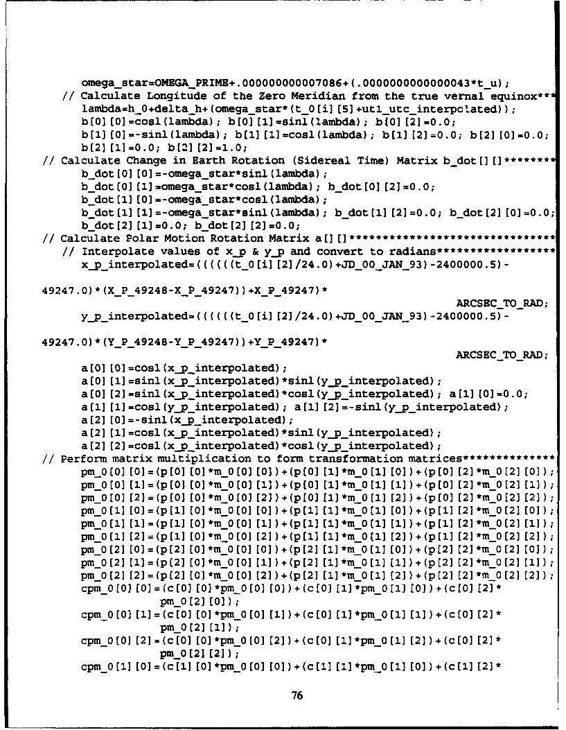
omega-star=OMEGAPRIME+ .000000000007086+ (.0000000000000043*tu);IICalculate Longitude of the Zero Meridian from the true vernal equinox**,lambda=hO+delta-h+ (omega-star* (t_0 (i](5]+utl-utc-interpcl~ated));b(0] (O]=cosl(lambda); b(0] (1]=sinl(lambda); b(0] (21=0.0;b(1] (O]=-sinl(lambda); b(1] (l1=cosl(lambda); b~i] (21=0.0; b[2] [0]=0.0;b(2] [11=0.0; b121 [21=1.0;
IICalculate Change in Earth Rotation (Sidereal Time) Matrix b-dot(](]~*******b -dot(0[] (]=-omega -star*sinl (lambda);b-dot[(01 (1=omega-star*cosl(lambda); b_dot (01 (21=0.0;b-dot(1] (0] =-omega -star*cosl (lambda);b-dot(1] (11=-omega-star*sinl(lambda); b_dot (11 21=0.0; b_dot(2] (01=0.0;b -dot [2] [11 =0. 0; b__dot([2] [21 =0. 0;
IICalculate Polar Motion Rotation Matrix a( ]***************
IIInterpolate values of x~p & y~p and convert to radians******************x-pinterpolated=((((((t_0(i] (2]/24.0)+JD_00_JAN_93) -2400000.5)-
49247.0)*(XP_49248-XP_49247))+XP_49247)*ARCSECTORAD;
y-pinterpolated=((((((t_0(i) (2]/24.0)+JD_00_JAN_93)-2400000.5)--
49247.0)*(YP_49248-YP_49247))+YP_49247)*ARCSECTORAD;
a[0] (01 =cosl (x~p interpolated);a [0] 1] =sinl (x-p interpolated) "sinl (y-pinterpolated);a(0] [2] =sinl (x-p-.interpolated) "cosl (y~p interpolated); a(1] (01=0.0;a [1][1] =cosl (y~p interpolated); a [1][2] =-sinl (y~p interpolated);a(2] (0]=-sinl (x~p interpolated);a (21 (1]=cosl (x-p interpolated) "sinl (y-pinterpolated);a (2] (2]=cosl (x-p interpolated) "cosl (y~p interpolated);
IIPerform matrix multiplication to form transformation matrices**************pm__10(01 [0 = (p (0] (0]*m_-0([0] [01) +(p (01 [1] m_-0([1] [0]) +(p (0] [21*m_-0([2] (0]) ;pm_0(01 Ill]=(p 10] [0] m_0([0] [1]) +(p (0] [1] mý_0(1] [1]) +(p (0] [2]"m_0(2] [1]) ;pm_0( 0] [2 = (p [0) [0]*m_-0[0] [2] ) +(p [0] [1]*m_-0([1] [21) +(p [0 (21*m_-0([2] (2]) ;pm_0O(1] [0 = (p (11 10]*m_-0([01 [0]) +(p (1] [1] mý_0(1] [0]) +(p([1] [2]"*mý_0(2] (0]) ;pm_0(1 (11Il= (p(I10] (01m_0(0] (1]) +(p([11 [1]*m_-0 (1] (1]) +(p (1] [21]"m_-0(21 [1]) ;pmi_0(11] [2] =(p [1] (0] *m_0(0]O (2] ) +(p Illl (1]"m_0[11 (2]) +(p [1] [21 *m_0[21 [2]) ;pm_0(12] [0 = (p [2] (01*m_-0([0] [01) +(p (2] [1] *m_0(11 [0]) +(p (21 (21 *m_-0(2] (01) ;pm_0([2] (1] =(p (2] [0] *m-0([0] [1]) +(p([2] [1]*m_-0([1] [1]) +(p(2 [2]"m1 Tt_0(2)1(11) ;pm_0( 2] [2 = (p (2] (0]*m_0([0] [2] ) +(p (2] [1]*m_0(1] (2]) +(p [2] (2]m_0(2] (2]) ;cpmýO([01 [0)]=(c([01 (0] *pmr_ [0(0 [0]) +(c [0) (1] "pm_ [(1] [0])+ (c(10] (21 *
pm_0( 2] (0]) ;cpmko (0] [1] =(c (01 (0] "pm_ 0(0] Ill) +(c([0] (1] "pm_ 0(1] Ill) +(c (0] (21 *
pmk_0(21(1]1) ;cpmo0(0] (2] =(c(0 (01 [0"pm_ 0(0] (2]) +(c([0] (1] "pm_ 0(1] [2]) +(c(0] (2]"*
pm_ 0[21 (2]) ;cpmo(01] (01=(c(1] (0] "pm_0(0] (0])+(c(1] (1] "pm 0(1~] (0])-.ic(1] (21*
76
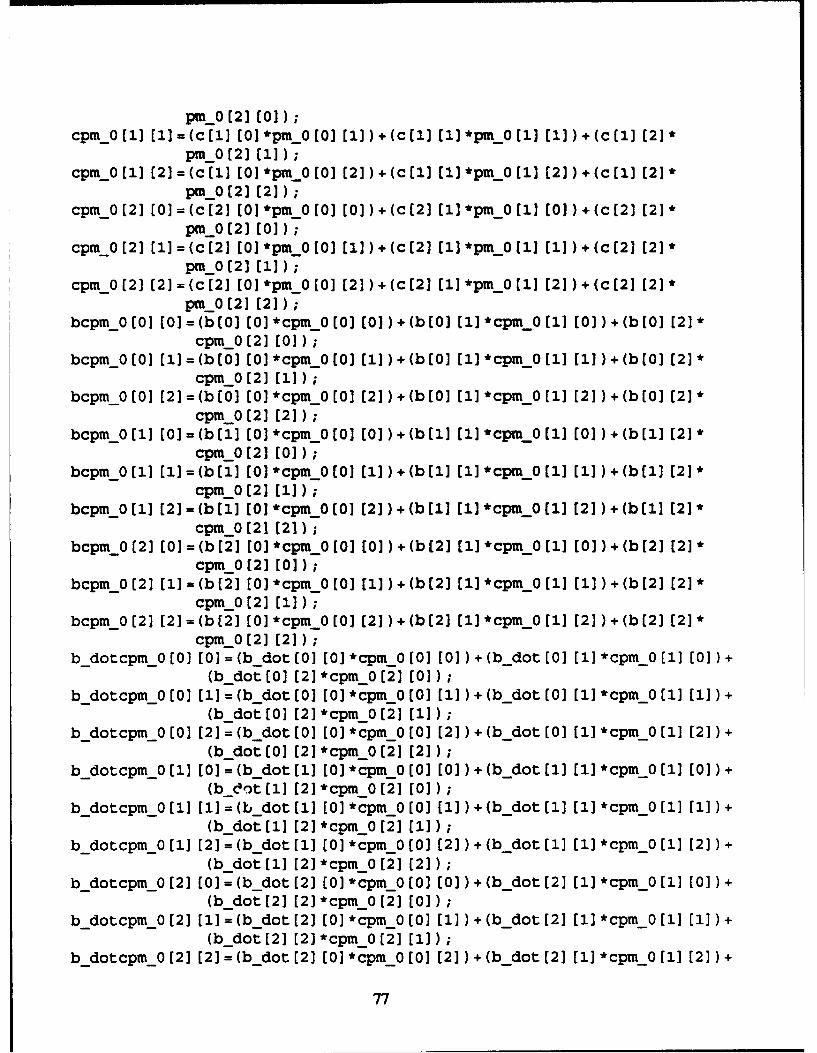
pm_0(21 (01);cpmýO [11 [1]=-(C (1] [0]*pmkO (01 (1]) +(C (1] [1] *pmO(1] (1] ) +(C (1 (21 *
pmý_0(2] (11) ;cpmo0(Ill 21 =(c(Ill (0] *pmR 0 (01 [2] ) +(c([1) (1] *pm 0(1l '2] ) +(c 1] (21*
pmý_0(2] (2])cpmkO([21 [0 = (c([2] [0] *pm_ 0(0] [0)]) +(c (2] [1] *pm_ 0(1] [01 ) +(c(2] (21*
pmý_0(2] ( 0]) ;cpmýO([2] (1 = (c([2] [0]*pmko([01 Ell) +(C([2] [11 *pmýO [1] (1] ) +(c([21 (21*
pmý_0 (2] [1])cpm-o(2] [2] =(c(2] [0)]*m-O (0] [2] ) +(c[2] (11 *pmýO Ill (2])+(C(2] [21*
pm_0(2] (2]);bcpmkO [0] [0 = (b (0] (01 *cpmko (0] (01 ) +(b (0] (1] *Cpm 0 (1] (0] ) + (b [0] [21 *
cpmýO (2] (0] ) ;bcpmkO (0] [1] =(b (0] (0] *cpm~ [0(0 [11 ) +(b([01 (1] *Cpk_0([11 [11) +(b (0] (21 *
cpmkO (2] (1]) ;bcpRO (0] [2 = (b([0] (0] *Cpm_ 0(0] [2]) +(b (0] [1] *Cpmý_0(1] [2] ) +(b(0] (21 *
cpmkO (21 (2]) ;bcpmRO([1] [0 = (b (1] (0] *cpm_ 0(0] [0] ) +(b([1 (1] *cpm 0(1l [0] ) +(b[1] (21 *
CpmrkO (21 (0]) ;bcpmkO (1] [1] =(b [1] [01*cpm 0(01 [1] ) +(b (1] (1] *cpý_0(1]l (1] ) +(b(1] (21 *
CpmýO (2] (11) ;bcpm-o( Il(21 =(b [1] (01 *CpmO([0] [2] ) +(b [1] [1] *Cpý_0([11 [2] ) +(b (11 (21 *
cpmo ( 21 (21 );bcpmkO([2] [0 = (b([2] (0] *cpm 0([0] [0] ) +(b[2] [11]*Cpmk_0(1] (0] ) +(b([2] (21 *
CpmlkO 12] (0]) ;bcpO (2] [1] =(b([21 [0] *cpmo (01 [1] ) +(b (2] [11*cpm_0(1] Il 1) + (b[2] (21 *
cpmýO (2] (1]1) ;bcpmýO (2] [2 = (b (2] [0)]*CpmýO(0] [2]) +(b([2] [1]*cpm_0O(1] [2] ) +(b (2 (21 *
cpmo (2](2]) ;b-dotcpmýO (0] (0 = (b-dot (0] [0] *cpmý_0(01 (01 ) +(b-dot [0] [1] *cpm_0(1l [1 0) +
(b-dot (0] (2] *Cpm (21(0]) ;b-dotcpmýO[0] [1] =(b-dot (0] [0)]*cpý_0([0] [1] ) +(b-dot(01 [1] *cpm_0O(1] [1]) +
(b-dot (0] ( 2] * cpmýO (2] (11) ;b-dotcpmýO[0] [2 = (b-dot[0] [0)]*Cpmr_O0(0 [2] ) +(b-dot [0] (1] *cpm_0O(1] (2 ) +
(b-dot (0] ( 21 * cpmO (2] (2]) ;b-dotcpmko([1] [01 =(b-dot([1] [0]*cpr_o 0( 0] 0) + (b-dot(Ill (1] *cpm_0( 1] [0 ) +
(b_&ot (1] (2] *CPmRO (2] (01) ;b-dotcpmýO[1) [1] =(b-dot (1] (01 *cpR_0([0] [11]) +(b-dot([1] [11]*Cpm0I 1] (1) +
(b-dot (1] (2] * Cpmko (21 (11) ;b-dotcpm0( 1] [2 = (b-dot (1] [0] *cpmý_0(0] (2] ) +(b-dot( l l *cpm_0(1l [1 2) +
(b-dot (11 21 *Cpmo (2] (2]);b-dotcpmko([2] (0 = (b-dot (2] (0] *cpm.0 (0] [0]) +(b-dot(21 [1] *Cpý_0([1] (0 ) +
(b-dot (2] (2] * CpmýO (2] (0] ) ;b-dotcpm0_(2] [11 =(b-dot([2] (0] *cpmý_0(0] [1]) +(b-dot([2] (1] *Cpý_0( IllIll) +
(b-dot [2] 12] * cpmkO (2] (11) ;b-dotcpmO (2] [2 = (b-dot([2] (0] *cpmk_0(0] [2] ) +(b-dot(2] (1] *Cpmý_0(1] (2 ) +
77
(b_dot (2] (2] *cpmn 0 2] [21) ;abcpm[O (0 [0]=-(a[(0] (0]*bcpmO[0) [0] )+(a [0] [1] *bcpmO[0 1] [01 )+(a (0] [21
bcpmkO 12] [0]) ;abcpmo0[0] [1]=(a[0] [0]*bcpm_0[0] [1])+(a[0] (1]*bcpm_0[1] (1])+(a[0] [21*
bcpmrkO 12] [11) ;abcpm-O (01 (2] = (a (0] [0] *bcpm 0O (0] [2] ) + (a (0] [1] *bcpm_ 0(1] (2] ) + (a [0] (21 *
bcpmO [2] (21) ;abcpmO [1] [0] = (a (1] (0] *bcpm 0 [0] (0] ) + (a (1] [1] *bcpmO [1] [0] ) + (a (1] [2] *
bcpmykO (2] [0]) ;abcpmO [1] [1] - (a [1] [0] *bcpm, 0 [0] [1] ) + (a (1] [1] *bcpmo [0 [1]Il ) + (a [1] (2] *
bcpmO (2] [ll]);abcpmkO[(1] [2 = (a [1] [0] *bcpmO(0] [2] ) +(a [11 [1] *bcpm 0[1) [2] ) +(a[(11 [21 *
bcpmtkO [2] [2]) ;abcpm-O[21 [0 = (a[(21 [01 *bcpm_ 0[0) [0) ) +(a [2] [1] *bcpm 0 [11[01 ) +(a[2) [21 *
bcpmO [2] [0]) ;abcpmo[0 21 [1)]=(a [2] [0] *bcpmo0[0] [1)]) +(a[2] [1] *bcpm_ 0I1] (11]) +(a12] (21 *
bcpmkO [2] [1 ]) ;abcpm.O[(2] [2 = (a[(2] [0] *bcpm 0 (0] [2] ) +(a[(2 [1] *bcpm 0[1] [2] ) +(a121 (21 *
bcpmrkO [2] [2]) ;ab_dotcpmo[0]0 [0]=(a[0] [0]*b-dotcpm o[0] [0])+(a[0] [1]*b-dotcpm. 01] [0])+
(a(0] [2]*b dotcpm_0(2]1[0]);ab_dotcpmo_[0] (1]=(a[0] [0]*b -dotcpm_0[0] [1])+(a[0] [1]*b-dotcpm_0[1] [1)+
(a[0] (2] *b dotcpm._0 (21(1l) ;ab_dotcpmo[O](0 [2]=(a[0] [0]*b-dotcpmo_[0] [2])+(a[0] [1]*b-dotcpm_0(1] [2])+
(a[(0] [2]*b dotcpm_0 (2] [2]) ;ab-dotcpmtk0[1] [0]=(a(1] [0]*b-dotcpm_0[0] [0])+(a[l] [1]*b-dotcpmo_[1] [0])+
(a [1] [2] *b dotcpmR_0 [2] [0]) ;ab-dotcpmo_[1] [1]=(a[1] [0]*b-dotcpm...0(0] [1])+(a[l] [1]*b-dotcpmo0[1] [l])+
(a[11] 12] *b dotcpmr_0(12] [11) ;ab_dot cpmýO 111 12 = (a[11 [0]*b -dotcpmo_(0] [2])+(a[1] C1]*b-dotcpmo-[1] [2])+
(a(1] [2]*b dotcpR_0(2] (2]);ab_dotcpm_0 [2] (0 = (a [2] [0]*b-dotcpmo[0](0 [0]) +(a (2] [1] *b-dotcpmko (1] (0])..
(a[12] 121*b dotcpm._0(12] [0]) ;ab_dotcpmo_[2] [1]=(a[2] [0]*b-dotcptuo[0] [1])+(a[21 [1]*b-dotcpmýO[1] [1])+
(a[12] 12]*b dotcpmO(12] [11) ;ab-dotcpmRo[(2] [2 = (a[(2] [01*b-dotcpm-O (0] [21)+ (a[(2] (1] *b-dotcpmko [11 [2])+
(a[12] 121*b dotcpm_0(12] [2])IITranspose the transformation mtie*******************
abcpmRO transposeO [0] [0 =abcpmý_O0(01(0];abcpmýO~transpose[10 [1J =abcpk_0(1 [1 0];abcpmrýo transpose [0] [2] =abcpmý_0(2][0];abcpm-o transpose [1][0] =abcpm_0(0] [1];abcpmO~transpose[1][l1]=abcpm_ 0(1][1];abcpm-o transpose [1][2] =abcpm_0(2] (1];abcpm~o transpose [2][0] =abcpm_0 [0] [2];abcpm-o transpose[2(2[1] =abcpm_0(1] [2];
78
abcpm O_transpose(2] [2] abcpm. [(21 [2];ab_dotcpmO transpose (01 [01-ab_dotcpin_ [0] [0];ab-dotcpmO transpose[(01 [1-ab-dotcpm_0(11 [0];ab-dotcpmo transpose [01 [21-ab_dotcpmO[21 [01;ab_dotcpmO transpose (11[01-ab -dotcpmO[01 [1];ab -dotcpm-o transpose l(11 [1-ab -dotcpm_0[1] [1];ab -dotcpm-o-transpose [11 21 -ab -dotcpm_0[(2][(1];ab -dotcpmOtranspose[2][01-ab dotcpm_0(01(2];ab -dotcpmO transpose (21 [lI-ab~dotcpm 011] [2];ab -dotcpmýO~transpose[2 [21 =ab-dotcpmO0[2] [2];
IIPerform ECEF_-WGS_-84 to ECIM50 position coordinate transformation**********v_1(i] [0]=(abcpm-Otranspose(01 [01*v_0[i1 [0])+(abcpm~o_transpose[0] [11*
vý_0[iI [l1)+(abcpm_0_transpose[01 [2]*v_0[i][2]);v_1(i] [l]=(abcpm-O-transpose[1] [0]*vO~i] [01)+(abcpm O_transpose~ll [11*
vý_0[il[11)+(abcpm_0O_transpose(l1[2]*v_0(i][21);v_1(i] (21=(abcpm-O-transpose[2] (01*vO~i] (0])+(abcpmO_transpose[21 [11*
vO~i][l1)+(abcpm_0_transpose[2][21*vO~il [21);//Perform ECEF_-WGS_84 to ECIM50 velocity coordinate transformation**********
v-l~i] (3]=(ab dotcpm_0_transposeCO] [0]*v_0(i][0])+(ab -dotcpmR_0_transposeCO] [l]*vO~i] [l1)+(ab dotcpm_0_transpose[01 [2]*vý_0[i](21)+(abcpmO~transposeL0] [01*v_0[Oil [31)+(abcpm O_transpose[0] [11*vý_0(il[41)+(abcpm_0_transpose[0][2]*v_0[i][5]);
v_1[i] (4]=(ab -dotcpmR_0_transpose~l] [01*vO 0i] [01)+(ab -dotcpm_-0_transposell[1] l*vO1i] [l)+(ab -dotcpm_0_transpose~l] (21*v%_0(i] (2])+(abcpmo Otranspose (1][0] *v_0Ci](3] ) +(abcpm O_transpose [1](1] *v_0(i] [41)+(abcpm_0_transpose~l] [2]*v_0[i] [5]);
v-l~i] [5]=(ab dotcpm_0_transpose[2] [O]*vO~i][01-)+(ab -dotcpmR_0_transpose[2] (1]*vO i] [1])+(ab -dotcpmR_0_transpose[2] (2]*vO i] [2])+(abcpmo~transpose[21 [0]*v_O~il (3])+(abcprn,.O_transpose(2] [11*vý_0[i] (4])+(abcpm_0_transpose[2] (2]*v_0[i] [5]);
1/Write status information to an external fileif((j=fopen(I'statout.O01","a"))==NULL)
fclose(j);nerror("lunable to open statout.O01 in maino");
if (i<l)
long double te..,tl, test2, test3, test41 test5, test6, test7, testS, test9;long double testlO, testili,testl2,testl3, testl4, testl5, testl6, testl7;testl=xypinterpolated/ARCSECTORAD;test2=y~pinterpolated/ARCSECTORAD;test3=-lambda/DEGTORAD;
79
test4n-epsilon-bar/DBGTOR.AD;testS~delta~psi/ARCSBCTORAD;test6.epsilon/DEGTO -RAD;test7=zeta/ARCSSCTO6 -RAD;test8=-theta/ARCSBCTOR.AD;test9=z/ARCSECTOR.AD;fprintf(j,"Rotate about the Y1 axis by V 16.l3Lf\".\n",testl);fprintf(j. "Rotate about the X2 axis by % 16.l3Lf\".\n",test2);fprintf(j,"Rotate about the Z3 axis by V 16.l3Lf degrees.\n",test3);fprintf(j,"Rotate about the X4 axis by t 16.l3Lf degrees.\n",test4);fprintf(j,"Rotate about the Z5 axis by t 16.l3Lf\"'.\n",test5);fprintf(j,"Rotate about the X6 axis by t 16.l3Lf degrees.\n",test6);fprintf(j,"Rotate about the Z7 axis by t 16.l3Lf\".\n",test7);fprintf(j,"Rotate about the YS axis by V 16.l3Lf\".\n",test8);fprintf(j,"Rotate about the Z9 axis by V 16.l3Lf\".\n",test9);fprintf(j,"Rotate about the Z10 axis by -0.320288870000 degrees\n");fprintf(j,"Rotate about the Y11 axis by 0.278405860000 degrees.\n");fprintf(j,"Rotate about the Z12 axis by -0.320381690000 degrees.\n");
if (fclose (j) ==EOF)
nerror("unable to close statout.001 in maino");
IIWrite ECIM50 state vectors to an external fl**************if( (j=fopen("'stateout.O01", "w"))=-NULL)
fclose(j);nerror("lunable to open stateout.00l in maino");
for(i=0;i<NUMBEROFVECTORS;i++)
fprintf(j,"tLf t .l2Le t .l2Le t .12Le\n t .l2Le t .l2Le I.l2Le\n",t_0[i] [2],v_1(iJ [0],vý_1(il] []v_l~i][2],v_1[](i3],vý_1[i] (4,vý_1[l [S]);
if (fclose(j) ==EOF)
nerror("unable to close stateout.001 in maino");I
IIWrite ECEFWGS_84 state vectors in Kalman Filter input file formnat*********if( (j=fopen("svO.001"1, "w") )==NULL)
fclose(j);nerror("unable to open sv0.00l in maino");
80
for(i=0;icNUMBEROFVNCTOR.S;i++)
int minutes;long double seconds;minutes-(int) (tO~i] [51/60.0);seconds-tO~i] [5] -(60.0*(float)minutes);minutes-=((int) (t-O~i] [5]/3600.0) *60);if(i>0)
if((t_0[i] [0]-t_Oti-l1 COJ)>longest)
longest=t_0 (i] [0]-t_0[i-lI [0];printf ("\nVLf", longest);
fprintf(j,"td %15.2Lf V 15.6Lf %- 15.6Lf V 15.6Lf %- 12.6Lf %- 12.6Lf12 .6Lf\n",
minutes~seconds,v_-0[i][0J,vý_0[i]1l,vý_0[i][2l~v_0(i][31,v_0[(i] [4] , v_0i1] [5])
if (f close (j) --BOF)
nerror("unable to close svO.00l in maino");
81
APPENDiX B
/ ************************************ */
1* This program compares state vectors and computes the magnitude of *1/* their position and velocity difference.
/* Author: LT Stephen P. Rehwald, USN *//* Date: 20 March 1994I* *//* Functions from "Numerical Recipes in C", Press, W.H., et al, *//* Cambridge University Press, 1988 were utilized in this program./* *//************************************************************************/*
/ ***********************************************************t************/
/* NUMBER OF VECTORS is the number of position/velocity vectors to/* process from the files used as input to this program. Each file */1* must, at a minimum, contain this number of vectors. STATEOUT.00i apO *//* REFTRAJ.001 specify the names of the input files. M5ODIFFS.001 *//* specifies the name of the output file. *1
#define NUMBEROFVECTORS 139
#include <math.h>#include <stdio.h>#include <stdlib.h>
void nerror(char*);
FILE *j,*k;int i;long double tO[NUMBER OF VECTORS][2],vdiff[NUMBEROFVECTORS][2];long double v_0[NUMBER_OF_VECTORS][6],v_1[NUMBEROFVECTORS][6];
/* *//* nerror is Numerical Recipes standard error handler*/1* */
void nerror(char error-text(])
fprintf(stderr,"Numerical Recipes run-time error... \n");fprintf(stderr,"%s\n",errortext);
82

fprintf(stderr,"...now exiting to system... \n");_exit(1) ;
void main(void)
IIRead GPS_-M50 and Reference Trajectory state vectors from external files****if((j=fopen("'stateout.0O1","r"))==NULL)
fclose(j);nerror("unable to open stateout.0O1 in maino");
if ((k=fopen ( "reftraj .001", "r")) --NULL)
fclose(k);nerror("lunable to open reftraj.0O1 in maino");
for(i=0;i<NUMBEROFVECTORS;i++)
fscanf (j, "ILf %-Le WLe %Le %Le *Le *Le\n",&t_0(iJ (0],&vO~i] (0],&v_-0 [i][1), &vý_0(i]([2),&_O (iH 3L, _O [iH[4],vO i]15]) ;
fscanf (k, "VLf VLe tLe VLe VLe tLe VLe\n", &t_0 Ci][1] ,&v_-1 (i] (0] ,&v-1(il](1, &v-1[i] [2 , &v-1[i[13], &vl1[i][141, &vl Ji][51);
I/if (i>0)
if(t_0(iHO]1!=t_0(i][1])
nerror("ltime element mismatch in maino");
if (fclose (j) ==EOF)
nerror("lunable to close stateout.001 in maino");
if (f close (k) ==EOF)
nerror("lunable to close reftraj.00l in maino");
IIMain loop to calculate time, rotation matrices, and transformations********for(i=0;i<NUMBEROFVECTORS;i+4-)
/1Compute the magnitude of the position difference***************************v-diff [i] [0]=sqrtl(powl((v_1(i] [01 -v_0(i] [0] ),2.0)+powl((v_ l[i] (1]-
vO[i]l][1) 2.0)+powl((v-l[il 2] -v 0(il(2]),2.0));
83
/1Compute the magnitude at the velocity difference***************************v-diff iJ [ll -sqrtl(powl((v I il (31-vO~il [3]),2.O)+powl((v-l~iJ [4]-
vO0(i] (41),2.O0).ipowl ((v.rl iH 51 -
IIWrite differences to an external fl*******************if( (j=fopen("m5Odiffs.O0l", "w"))..*NULL)
fclose(j);nerror("unable to open DIFFERENCEFILE in maino");
for(i=O;i<NUMBEROFVECTORS;i++)
fprintf (j. "%Lf t16.l3Lf%16.13Lf\n",t_O[i] [0],vý_diff[ii [0] ,v_diff(i] (1]);
if (fclose (j) ==EOF)
nerror(munable to close DIFFERENCEFILE in maino");
84
APPENDIX C
The plots appearing in this appendix depict the number of usable GPS satellites
being tracked by the recevier. If more than three usable satellites are being tracked, the
indication is given either that the receiver is doing position fixes, or that PDOP is too
high. VDOP, HDOP, and PDOP are also shown (PDOP is a combination of VDOP and
HDOP) at the corresponding times. The segment at the center (right to left) of each plot
corresponds to the data chosen for analysis in Chapter III, Table 3. For comparison pur-
poses the times shown in Figures 5-10 equate to times appearing on the TANSGRAPH
plots as follows:
* 6261.434514 hours is FRI:21:26:04.25* 6261.507708 hours is FRI:21:30:27.75
* 6261.893542 hours is FRI:21:53:36.75* 6261.988264 hours is FRI:21:59:17.75
* 6265.089236 hours is SAT:01:05:21.25* 6265.193264 hours is SAT:01:11:35.75
85
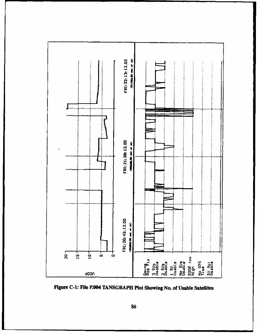
II_ a
...... I.... .... .. .......... . .. ............
L.6
0s.
.., .. .... ...... .... ...... . ... ... .. . .. ..... ....... ....
~4 .- 9
0 0
o- - 9. o.- L Li-0ýu iii 0h Lfl 00 M0P E t
00 In In Mf C3n. - . -.- > #AdOCIA C= cq = -4= = .C Zs- cn
Figure C-i: File P.004 TANSGRAPH Plot Showing No. of Usable Satellites
86
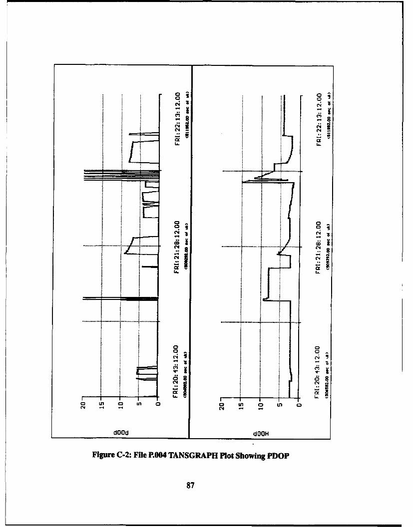
S~N
---- --- ...... ....... .....
= .... ................. ..
S........................... .
C),
- - . - -
* C41 C-
..* . .. *
a IX1 C3 tn 0: in• LO(3 n 03
C-4
dOOd dOOH
Figure C-2: File P.004 TANSGRAPH Plot Showing PDOP
87
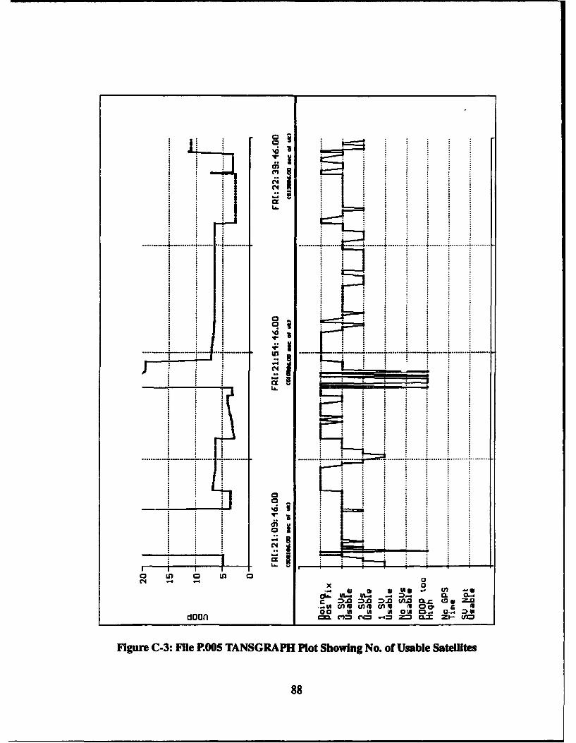
'CU
4.4
RI
LA.
............ .. ..... .. ............... ..........
0 LO 0 U) 0x
C :>a:. -. n CLC f 0ZM
."Mn U) Cn 0 -M 0
Figure C-3: Fie P.005 TANSGRAPH Plot Showing No. of Usable Sateliltes
88
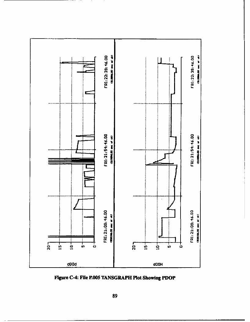
%00
N .4Ix-
In .....
8n
CK ex
....... ...... .... ........* -3
CI -6 --
doa 0,O
F*u -:Fl P.05 TASRP Po hwigP
89;'C
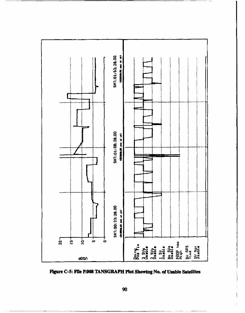
C4
U3
.4 .... ........... 4... 4.. ....... .... ....... - . . ...... ...........I
0
C4
tC4
a In C2 in
=>. ~f .C CII.. CL.C CD g Z
00 IA bi LA QOW _. 0..
Figure C-5: File P.008 TANSGRAPH Plot Showing No. of Usable Satellites
90
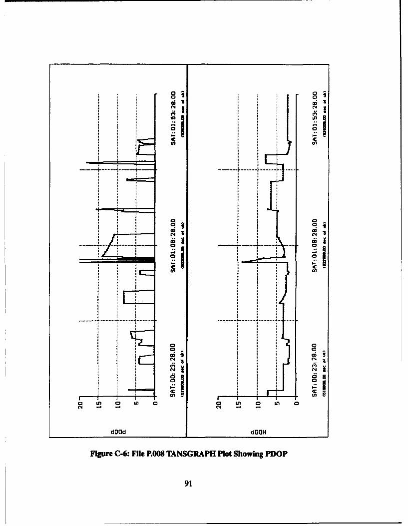
0
:1:1aii
C N
0 0
* .. 3
. . .; .
00 0
010
0 I- 0 0 Iin 0 Ln 0
dOOd dOcH
Figure C-6: File P.008 TANSGRAPH Plot Showing PDOP
91
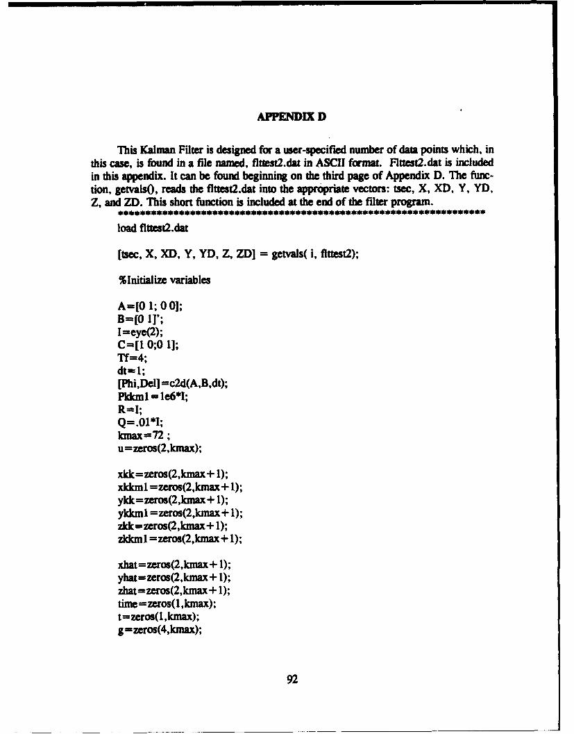
APPENDIX D
This Kalman Filter is designed for a user-specified number of data points which, inthis case, is found in a file named, flttestU.dat in ASCII format. Fl.test2.dat is includedin this appendix. It can be found beginning on the third page of Appendix D. The func-tion, getvalso, reads the flttest2.dat into the appropriate vectors: tsec, X, XD, Y, YD,Z, and ZD. This short function is included at the end of the filter program.
load flttest2.dat
[tsec, X, XD, Y, YD, Z, ZDJ = getvals( i, flttest2);
%Initialize variables
A=[O 1; 0 0];B=[O I]';If=eye(2);C=[1 0;0 1];Tf=4;dt= 1;[Phi,Del] =c2d(A,B,dt);Pkkml = le6*1;R=I;Q=.01*1;kmax=72;u=zeros(2,kmax);
xkk=zeros(2,knmax+ );xkkml =zeros(2,kmax+ 1);ykk=zeros(2,kmax+ 1);ykkml - zeros(2,kmax + 1);zkk=zeros(2,kmax+ 1);zkkml =zeros(2,kmax+ 1);
xhat=zeros(2,knax+ 1);yhat=zeros(2,knax+ 1);zhat=zeros(2,kmax+ 1);time =fzeros(l,kmax);t=zeros(1,kmax);g =zeros(4,kmax);
92
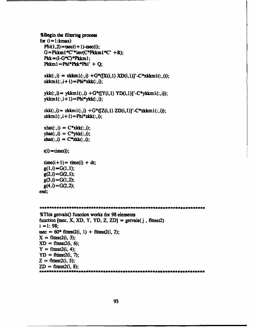
%Begin the filtering processfor (i -l:kmax)
Phi(l,2) -tse~i + )tci;G=Pkkml*C'*inv(C*Pkkml*C' +R);Pkk=dI-*C)*Pkkmi1;Pkinl=Phi*Pkk*Phi' + Q-,
xick(:,i) = xkicmI(:,i) +G*([X(i,l) XD(i,l)J'-C*xkkml(:,i));,xkknil(:,i+ l)=Phi*xkk(:,i);
ykk(: ,i) = ykkml(:,i) +G*([Y(i, 1) YD(i, l)J'-C'ykkml(: ,i));ykkmnl(:,i+ 1)=Phi"'ykk(:,i);
zkk(: ,i) = zkkmnl(: ,i) +G*([Z(i, 1) ZD(i, 1)J'-C*zkkml(: ,i));zkkznl(: ,i+1) =Phi*zkk(:,i);
xhat(:,i) = C~xkk(:,i);yhat(:,i) = C*ykk(:,i);zhat(:,i) = C~'zkk(:,i);
time(i+ 1) = time(i) + dt;
g(3,i) =G(1 ,2);g(4,i) =G(2,2);
end;
%Tis getvalsO function works for 98 elementsfuinction [tsec, X, XD, Y, YD, Z, ZDJ = getvals(j , flttest2)i=1: 98;
tsec = 60* flttest2(i, 1) + flttest2(i, 2);X = flttest2(i, 3);XD = flttest2(i, 6);Y = flttest2(i, 4);YD = flttest2(i, 7);Z = flttest2(i, 5);ZD = flttest2(i, 8);
93
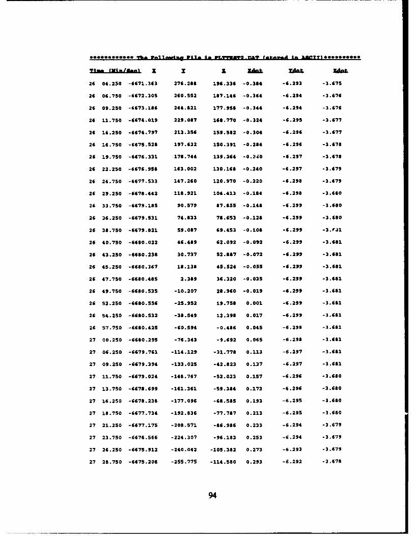
************ q~m 3e114ngw W41 IR IFLq*I DkY I mtawpA 41 kflITTI*O*OOOOgOO
26 04.250 -4671.363 276.288 199.336 -0.384 -6.293 -3.675
26 04.750 -6672.305 260.552 187.146 -0.364 -6.294 -3.676
26 09.250 -6673.186 244.821 177.958 -0.344 -6.294 -3.676
26 11.750 -6674.019 229.087 168.770 -0.324 -6.295 -3.677
26 14.250 -6674.797 213.356 159.582 -0.304 -6.296 -3.677
26 16.750 -6675.528 197.622 150.391 -0.284 -6.296 -3.678
26 19.750 -6676.331 178.744 139.364 -0.240 -6.297 -3.678
26 22.250 -6676.958 163.002 130.168 -0.240 -6.297 -3.679
26 24.750 -6677.533 147.260 120.970 -0.220 -6.298 -3.679
26 29.250 -6678.442 118.921 104.413 -0.184 -6.298 -3.680
26 33.750 -6679.185 90.579 87.855 -0.148 -6.299 -3.680
26 36.250 -6679.531 74.833 78.653 -0.128 -6.299 -3.680
26 38.750 -6679.821 59.087 69.453 -0.108 -6.299 -3.FJ1
26 40.750 -6680.022 46.489 62.092 -0.092 -6.299 -3.681
26 43.250 -6680.238 30.737 52.887 -0.072 -6.299 -3.681
26 45.250 -6680.367 18.138 45.524 -0.055 -6.299 -3.681
26 47.750 -6680.485 2.389 36.320 -0.035 -6.299 -3.681
26 49.750 -6680.535 -10.207 28.960 -0.019 -6.299 -3.681
26 52.250 -6680.556 -25.952 19.758 0.001 -6.299 -3.681
26 54.250 -6680.532 -38.549 12.398 0.017 -6.299 -3.681
26 57.750 -6680.425 -60.594 -0.486 0.045 -6.298 -3.681
27 00.250 -6680.295 -76.343 -9.692 0.065 -6.298 -3.681
27 06.250 -6679.761 -114.129 -31.778 0.113 -6.297 -3.681
27 09.250 -6679.394 -133.025 -42.823 0.137 -6.297 -3.681
27 11.750 -6679.024 -148.767 -52.023 0.157 -6.296 -3.680
27 13.750 -6678.699 -161.361 -59.384 0.173 -6.296 -3.680
27 16.250 -6678.238 -177.096 -68.585 0.193 -6.295 -3.680
27 18.750 -6677.734 -192.836 -77.787 0.213 -6.295 -3.680
27 21.250 -6677.175 -208.571 -86.986 0.233 -6.294 -3.679
27 23.750 -6676.566 -224.307 -96.183 0.253 -6.294 -3.679
27 26.250 -6675.912 -240.042 -105.382 0.273 -6.293 -3.679
27 28.750 -6675.208 -255.775 -114.580 0.293 -6.292 -3.678
94
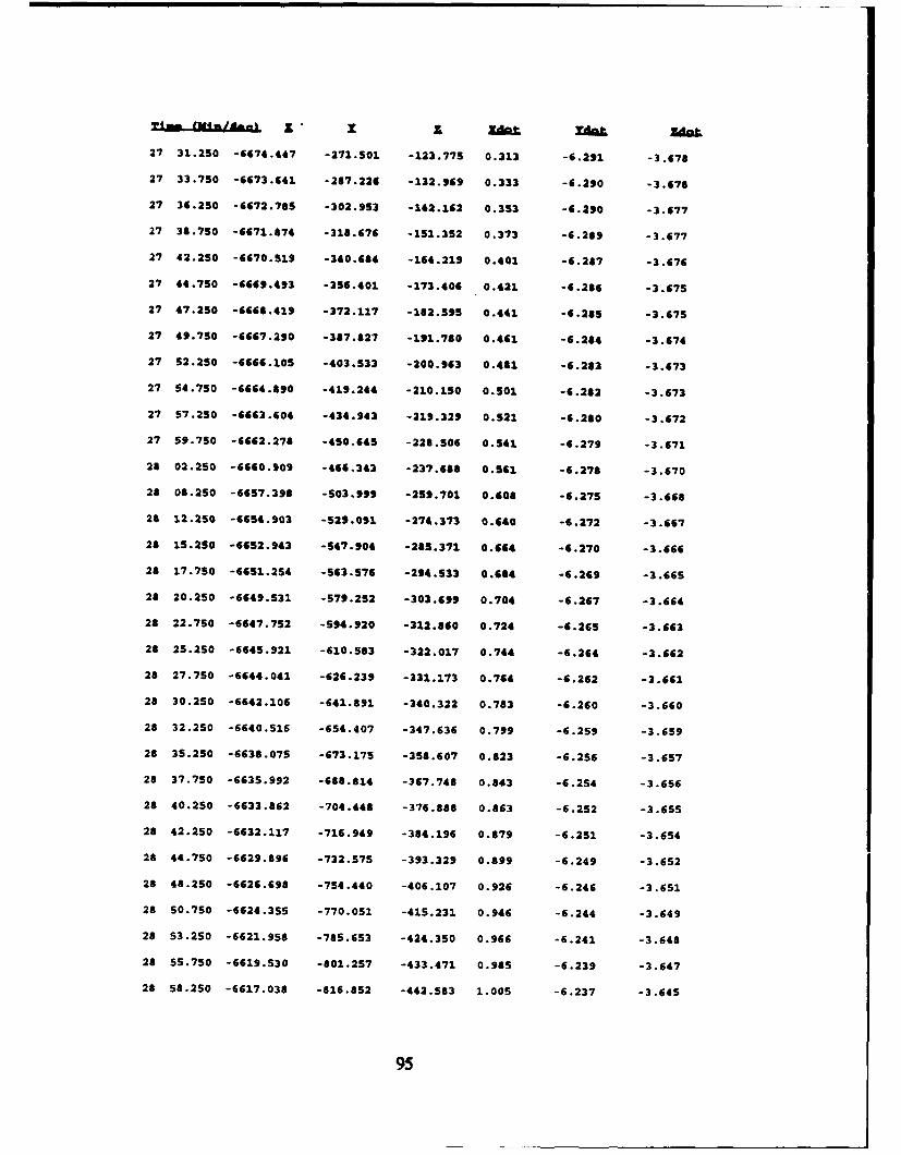
Stn� f •M u" x UAL ZAAi. JMat.
27 31.250 -6674.447 -271.s01 -123.775 0.313 -6.291 -3.678
27 33.750 -6673.641 -257.226 -132.969 0.333 -6.290 -3.676
27 36.2S0 -6472.785 -302.9S3 -142.162 0.353 -4.290 -3.677
27 38.750 -6671.874 -318.676 -151.352 0.373 -6.289 -3.677
27 42.250 -6670.519 -340.684 -164.219 0.401 -6.287 -3.676
27 44.750 -6649.493 -356.401 -173.406 0.421 -6.286 -3.675
27 47.250 -6668.419 -372.117 -182.595 0.441 -6.285 -3.675
27 49.750 -6667.290 -387.827 -191.780 0.461 -6.284 -3.674
27 52.250 -6666.105 -403.533 -200.963 0.481 -6.283 -3.673
27 54.750 -6664.890 -419.244 -210.150 0.501 -6.282 -3.673
27 57.250 -6463.604 -434.943 -219.329 0.521 -6.280 -3.672
27 59.750 -6662.278 -450.645 -228.506 0.541 -6.279 -3.671
28 02.250 -6660.909 -466.343 -237.688 0.56l -6.278 -3.670
28 08.250 -6657.398 -S03.999 -259.701 0.608 -6.275 -3.668
28 12.230 -6654.903 -529.091 -274.373 0.640 -6.272 -3.667
28 15.250 -6652.943 -547.904 -285.371 0.664 -6.270 -3.666
28 17.750 -6651.254 -563.576 -294.533 0.644 -6.269 -3.665
28 20.250 -6649.531 -579.252 -303.699 0.704 -6.267 -3.664
28 22.750 -6647.752 -594.920 -312.860 0.724 -6.265 -3.663
28 25.250 -6645.921 -610.583 -322.017 0.744 -6.264 -3.662
28 27.750 -6644.041 -626.239 -331.173 0.764 -6.262 -3.661
28 30.250 -6642.106 -641.891 -340.322 0.783 -6.260 -3.660
28 32.250 -6640.S16 -654.407 -347.636 0.799 -6.259 -3.659
28 35.250 -6638.075 -673.175 -358.607 0.823 -6.256 -3.657
28 37.7SO -6635.992 -688.814 -367.748 0.843 -6.254 -3.656
28 40.250 -6633.862 -704.448 -376.888 0.863 -6.252 -3.655
28 42.250 -6632.117 -716.949 -384.196 0.879 -6.251 -3.654
28 44.750 -6629.896 -732.575 -393.329 0.899 -6.249 -3.652
28 48.250 -6626.698 -754.440 -406.107 0.926 -6.246 -3.651
28 50.750 -6624.355 -770.051 -415.231 0.946 -6.244 -3.649
28 53.250 -6621.958 -785.653 -424.350 0.966 -6.241 -3.648
28 55.750 -6619.530 -801.257 -433.471 0.985 -6.239 -3.647
28 58.250 -6617.038 -816.852 -442.583 1.005 -6.237 -3.645
95
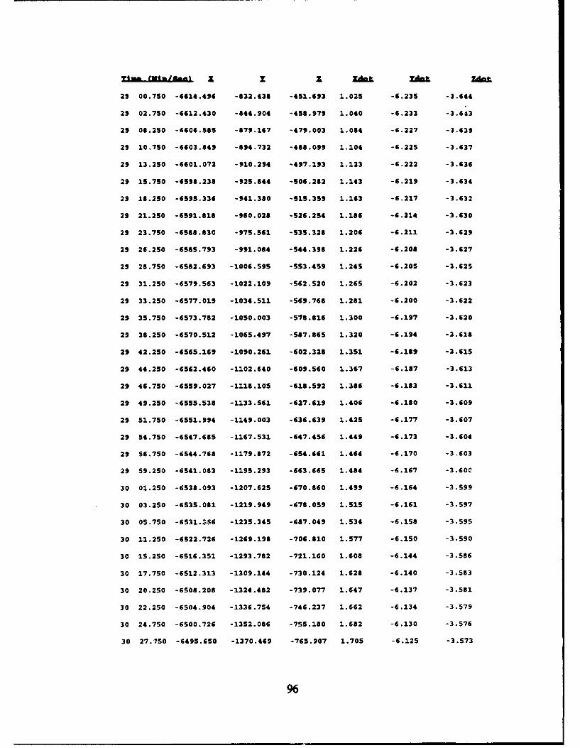
Sz I I ZdaL Xd".L Zak
29 00.750 -6614.496 -632.438 -451.693 1.025 -4.235 -3.644
29 02.750 -6812.430 -844.904 -458.979 1.040 -6.233 -3.6;3
29 08.250 -6606.585 -879.167 -479.003 1.084 -6.227 -3.639
29 10.750 -6603.849 -894.732 -488.099 1.104 -6.225 -3.637
29 13.250 -6601.072 -910.294 -497.193 1.123 -6.222 -3.636
29 15.750 -6598.238 -925.844 -506.282 1.143 -6.219 -3.634
29 18.250 -6595.336 -941.380 -515.359 1.163 -6.217 -3.632
29 21.250 -6591.818 -960.028 -526.254 1.186 -6.214 -3.630
29 23.750 -6588.830 -975.561 -535.328 1.206 -6.211 -3.629
29 26.250 -6585.793 -991.084 -544.398 1.226 -6.208 -3.627
29 28.750 -6582.693 -1006.595 -SS3.459 1.245 -6.205 -3.625
29 31.250 -6579.563 -1022.109 -562.520 1.265 -6.202 -3.623
29 33.250 -6577.019 -1034.511 -569.768 1.281 -6.200 -3.622
29 35.750 -6573.782 -1050.003 -578.816 1.300 -6.197 -3.620
29 38.250 -6570.512 -1065.497 -587.865 1.320 -6.194 -3.618
29 42.250 -6565.169 -1090.261 -602.328 1.351 -6.189 -3.615
29 44.250 -6562.460 -1102.640 -609.560 1.367 -6.187 -3.613
29 46.750 -6559.027 -1118.105 -618.592 1.386 -6.183 -3.611
29 49.250 -6555.538 -1133.S61 -627.619 1.406 -6.180 -3.609
29 51.750 -6551.994 -1149.003 -639.639 1.425 -6.177 -3.607
29 54.750 -6547.685 -1167.531 -647.456 1.449 -6.173 -3.604
29 56.750 -6544.768 -1179.872 -654.661 1.464 -6.170 -3.603
29 59.250 -6541.083 -1195.293 -663.665 1.484 -6.167 -3.60C
30 01.250 -6538.093 -1207.625 -670.860 1.499 -6.164 -3.599
30 03.250 -6535.081 -1219.949 -678.059 1.515 -6.161 -3.597
30 05.750 -6531.ZS6 -1235.345 -687.049 1.534 -6.158 -3.595
30 11.250 -6522.726 -1269.198 -706.810 1.577 -6.150 -3.S90
30 15.250 -6516.351 -1293.782 -721.160 1.608 -6.144 -3.586
30 17.750 -6512.313 -1309.144 -730.124 1.628 -6.140 -3.583
30 20.250 -6508.208 -1324.482 -739.077 1.647 -6.137 -3.581
30 22.250 -6504.904 -1336.754 -746.237 1.662 -6.134 -3.579
30 24.750 -6500.726 -1352.086 -755.180 1.682 -6.130 -3.576
30 27.150 -6495.650 -1370.469 -765.907 1.705 -6.125 -3.573
LIST OF REFERENCES
Defense Mapping Agency, Report 8350.2, Department of Defense World Geodetic Sys-tem 1984. Its Definition and Relationships with Local Geodetic Systems, pp.2-1, 1987.
Handout from AA 3276, Introduction to Avionics, class taught by Dr. I.I. Kaminar,"Design and performance analysis of Kalman filters," Naval Postgraduate School, Sep-tember 1993.
Kachmar, P.M., Chu, W., Neirinckx, P.and Montez, M.,"U.S. Space Shuttle: Inte-grated GPS Navigation Capability," Proceedings of ION GPS-93, Sixth InternationalTechnical Meeting, Salt Lake City, Utah, September 1993, pp.313-326.
Leewen, A.V., Rosen, E., and Carrier, L., The Global Positioning System and ItsApplication in Spacecraft Navigation, Journal of the Institute of Navigation, pp. 118-135,Summer 1979.
Naval Postgraduate School, Advanced Avionics Technology, Kaminar, I.I., (PrincipleInvestigator), pp. 117-138 and pp. 167-169.
NAVSTAR-GPS Joint Program Office, NA VSTAR GPS User Equipment Introdution(For Official Use Only), pp.3-1 to 3-9 and pp.8-i to 8-7, U.S. Air Force Space SystemsDivision, 1990.
Milliken, R.J., and Zoller, C.J., "Principle of Operation of NAVSTAR and SystemCharacteristics, " Global Positioning System, Vol. I, Washington, D.C., Institute ofNavigation, 1980.
Saunders, P.E.and others, "The First Flight Tests of GPS on the Space Shuttle," paperpresented at the Institute of Navigation Convention, San Diego, California, 24 January1994.
97
BIBLIOGRAPHY
The Astronomical Almanac for the Year..., Washington: Government Printing Office.
Chaffee, J.W., Zare, K., and Pojman, J., "Autonomous Navigation for COMET withGPS," Proceedings of ION GPS-93, Sixth International Technical Mecting, Salt LakeCity, Utah, September 1993, pp.293-297.
Duiven, E.M., Connolly, P.E., and Alfriend, K.T., "Satellite Tracking Using GPSMeasurements," IEEE, 1978.
Hashida, Y., and Unwin, M.J., "Satellite Attitude From a Single GPS Antenna," Pro-ceedings of ION GPS-93, Sixth International Technical Meeting, Salt Lake City, Utah,September 1993, pp.355-363.
Hofmann-Wellenhof, B., Lichtenegger, H., and Collins, J., Global Positioning SystemTheory and Practice, Second Edition, Springer-Verlag Wien New York, 1993.
McCarthy, D., Carter, M.S., and Luzum, B.J., Operational Prediction of the Earth'sOrientation in the International Earth Rotation Service (IERS) Reference Frame, U.S.Naval Observatory, Washington, D.C., c. 1991.
NASA Technical Memorandum, Report X-58153, Coordinate Systems for the SpaceShuttle Program, October 1974.
Notes and data from Ed Brown of Rockwell Shuttle Navigation at NASA Johnson SpaceCenter.
Notes and data from Penny Saunders of NASA Johnson Space Center.
Seidelmann, K.P.(editor), Explanatory Supplement to the Astronomical Almanac (Rev.Ed.), Mill Valley, CA: University Science Books, 1992.
Taff, L. G., Computational Spherical Astronomy, New York: Wiley, 1981.
Tang, W., and Howell, G., "Integrated GPS/INS Kalman Filter ImplementationIssues," Proceedings of ION GPS-93, Sixth International Technical Meeting, Salt LakeCity, Utah, September 1993, pp. 2 17-224 .
TANS QUADREX Space Configuration GPS Receiver Interface Control Document, PartNumber 17035-SP, Revision E, Trimble Navigation Limited, Sunnyvale, CA, 1992.
Zyla, L.V., and Montez, M.N., "Use of Two GPS Receivers in Order to Perform SpaceVehicle Orbital Rendezvous," Proceedings of ION GPS-93, Sixth International Techni-cal Meeting, Salt Lake City, Utah, September 1993, pp.30 1-3 12 .
98
INITIAL DISTRIBUTION LIST
1. Defense Technical Information Center 2Cameron StationAlexandria, Virginia 22304-6145
2. Dudley Knox Library 2Naval Postgraduate SchoolCode 52Monterey, California 93943-5002
3. CDR Randy Wight 1Naval Postgraduate SchoolCode SP/WtMonterey, California 93943-5002
4. Professor 1. M. Ross 1Naval Postgraduate SchoolCode AA/ROMonterey, California 93943-5002
5. Prfesor Don Danielson INaval Postgraduate SchoolCode MA/DDMonterey, California 93943-5002
6. Commander 1Naval Space CommandDahlgren, Virginia 22448
7. LT Lee Barker 1SPAWAR 402451 Crystal Dr.Arlington, Virginia 22245-5200
8. Dr. Jim Newman 1NASA Johnson Space CenterMail Code CBHouston, Texas 77058
9. Flora Lowes 1NASA Johnson Space CenterMail Code DM4Houston, Texas 77058
99
10. Penny SaundersNASA Johnson Space CenterMail Code EE6Houston, Texas 77058
11. Stephen RehwaldP.O. Box 1129San Bernardino, California 92402-1129
12. Carolyn Tyler122% Dunecrest Ave.Monterey, California 93940
100