Multivariate spectroscopic methods for

the analysis of solutions

Kent Wiberg

(mAU)

(min)

Time (min)

Wav

elen

gth

(nm

)

(nm)

Department of Analytical Chemistry

Arrhenius Laboratory

Stockholm University

2004

PhD Thesis Multivariate spectroscopic methods for the analysis of solutions Kent Wiberg Department of Analytical Chemistry Stockholm University SE-106 91 Stockholm Sweden Kent Wiberg, 2004 ISBN 91-7265-789-8 Akademitryck AB, Edsbruk

“In my opinion, analyses in the future will consist of linked individual methods evaluated using chemometric methods with the help of integrated data evaluating systems.” Josef F. K. Huber

Multivariate spectroscopic methods for the analysis of solutions

Kent Wiberg Department of Analytical Chemistry, Stockholm University, SE-106 91 Stockholm, Sweden Abstract In this thesis some multivariate spectroscopic methods for the analysis of solutions are proposed. Spectroscopy and multivariate data analysis form a powerful combination for obtaining both quantitative and qualitative information and it is shown how spectroscopic techniques in combination with chemometric data evaluation can be used to obtain rapid, simple and efficient analytical methods. These spectroscopic methods consisting of spectroscopic analysis, a high level of automation and chemometric data evaluation can lead to analytical methods with a high analytical capacity, and for these methods, the term high-capacity analysis (HCA) is suggested. It is further shown how chemometric evaluation of the multivariate data in chromatographic analyses decreases the need for baseline separation. The thesis is based on six papers and the chemometric tools used are experimental design, principal component analysis (PCA), soft independent modelling of class analogy (SIMCA), partial least squares regression (PLS) and parallel factor analysis (PARAFAC). The analytical techniques utilised are scanning ultraviolet-visible (UV-Vis) spectroscopy, diode array detection (DAD) used in non-column chromatographic diode array UV spectroscopy, high-performance liquid chromatography with diode array detection (HPLC-DAD) and fluorescence spectroscopy. The methods proposed are exemplified in the analysis of pharmaceutical solutions and serum proteins. In Paper I a method is proposed for the determination of the content and identity of the active compound in pharmaceutical solutions by means of UV-Vis spectroscopy, orthogonal signal correction and multivariate calibration with PLS and SIMCA classification. Paper II proposes a new method for the rapid determination of pharmaceutical solutions by the use of non-column chromatographic diode array UV spectroscopy, i.e. a conventional HPLC-DAD system without any chromatographic column connected. In Paper III an investigation is made of the ability of a control sample, of known content and identity to diagnose and correct errors in multivariate predictions something that together with use of multivariate residuals can make it possible to use the same calibration model over time. In Paper IV a method is proposed for simultaneous determination of serum proteins with fluorescence spectroscopy and multivariate calibration. Paper V proposes a method for the determination of chromatographic peak purity by means of PCA of HPLC-DAD data. In Paper VI PARAFAC is applied for the decomposition of DAD data of some partially separated peaks into the pure chromatographic, spectral and concentration profiles.

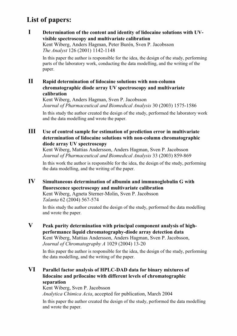
I Determination of the content and identity of lidocaine solutions with UV-visible spectroscopy and multivariate calibration Kent Wiberg, Anders Hagman, Peter Burén, Sven P. Jacobsson The Analyst 126 (2001) 1142-1148

In this paper the author is responsible for the idea, the design of the study, performing parts of the laboratory work, conducting the data modelling, and the writing of the paper.

II Rapid determination of lidocaine solutions with non-column

chromatographic diode array UV spectroscopy and multivariate calibration Kent Wiberg, Anders Hagman, Sven P. Jacobsson Journal of Pharmaceutical and Biomedical Analysis 30 (2003) 1575-1586

In this study the author created the design of the study, performed the laboratory work and the data modelling and wrote the paper.

III Use of control sample for estimation of prediction error in multivariate

determination of lidocaine solutions with non-column chromatographic diode array UV spectroscopy Kent Wiberg, Mattias Andersson, Anders Hagman, Sven P. Jacobsson Journal of Pharmaceutical and Biomedical Analysis 33 (2003) 859-869

In this work the author is responsible for the idea, the design of the study, performing the data modelling, and the writing of the paper.

IV Simultaneous determination of albumin and immunoglobulin G with

fluorescence spectroscopy and multivariate calibration Kent Wiberg, Agneta Sterner-Molin, Sven P. Jacobsson Talanta 62 (2004) 567-574

In this study the author created the design of the study, performed the data modelling and wrote the paper.

V Peak purity determination with principal component analysis of high-

performance liquid chromatography-diode array detection data Kent Wiberg, Mattias Andersson, Anders Hagman, Sven P. Jacobsson, Journal of Chromatography A 1029 (2004) 13-20

In this paper the author is responsible for the idea, the design of the study, performing the data modelling, and the writing of the paper.

VI Parallel factor analysis of HPLC-DAD data for binary mixtures of

lidocaine and prilocaine with different levels of chromatographic separation Kent Wiberg, Sven P. Jacobsson Analytica Chimica Acta, accepted for publication, March 2004

In this paper the author created the design of the study, performed the data modelling and wrote the paper.

List of papers:

Abbreviations and symbols

CDS Chromatographic data system CV Cross validation DAD Diode array detection/detector EEM Excitation-emission matrix EFA Evolving factor analysis HCA High Capacity Analysis IgG Immunoglobulin G MLR Multiple linear regression NIPALS Non-linear iterative partial least squares OSC Orthogonal signal correction PARAFAC Parallel factor analysis PBS Phosphate-buffered Saline PC Principal component PCA Principal component analysis PCR Principal component regression PLS Partial least squares regression PRESS Prediction error sum of squares RMSEP Root mean square error of prediction RSD Relative standard deviation RSEP Relative standard error of prediction RS Chromatographic resolution SS Sum of squares UV Ultraviolet UV-Vis Ultraviolet-visible

a Number of PCs m Number of observations n Number of variables t Score vector p Loading vector X Matrix of x-variables Y Matrix of dependent y-variables E Residual matrix λ Eigenvalue s Standard deviation s0 Pooled residual standard deviation si Absolute residual standard deviation of a single observation eik Residual of observation k for variable i β Regression coefficient in experimental design

Table of contents 1. Introduction 1

1.1 Objective 3 1.2 Pharmaceutical analysis 3 1.3 Summary of papers 4

2. Theory 6

2.1 Spectroscopy 6 2.1.1 Ultraviolet-visible absorption spectroscopy 9 2.1.2 Diode array detection 12 2.1.3 Fluorescence spectroscopy 14

2.2 Liquid chromatography 18

2.3 Chemometrics 20 2.3.1 Dimensionality of analytical chemical data 21 2.3.2 The model concept 23 2.3.3 Validation 24

2.4 Experimental design 27

2.5 Multivariate data analysis 30

2.5.1 Multivariate calibration 32 2.5.2 Multivariate curve resolution 34 2.5.3 Principal component analysis 35

2.5.4 SIMCA classification 37 2.5.5 Partial least squares regression 39 2.5.6 Parallel factor analysis 41

3. Discussion 42 3.1 Paper I 42 3.2 Paper II 45 3.3 Paper III 48 3.4 Paper IV 52 3.5 Paper V 54 3.6 Paper VI 59 4. Conclusions 62 5. Acknowledgements 64 6. References 65

1

1. Introduction The science of analytical chemistry can be described in simplified terms as the process of obtaining knowledge of a sample by chemical analysis of some kind. The sample under investigation may consist of any solid, liquid or gaseous compound and the result of the analysis is data of some kind that is related to the initial question raised about the sample. From the data obtained in the analysis some knowledge about the sample can be extracted. This knowledge may be either qualitative or quantitative (or both). Examples of qualitative information are types of atoms, molecules, functional groups or some other qualitative measure, while the quantitative information provides numerical information such as the content of different compounds in the sample. The qualitative information thus answers the question what? while the quantitative information is more related to the question how much?. At the beginning of the 19th century performing chemical analyses was a tedious and labour-intensive task. Analytical instruments were primitive and most analyses were carried out using wet chemistry. Furthermore, the results of an analysis were often a change in the colour of a reagent, the boiling point, the solubility, the odours, the optical activity and suchlike. In the last fifty to sixty years, however, the enormous developments that have taken place in analytical chemical techniques, microelectronics and computers have increased and revolutionised the scope for performing analytical chemical analyses. Nowadays an analytical chemical analysis generally includes some sort of analytical instrument that performs the actual analysis, while the data processing and instrument control are taken care of by software run on a computer. Hence it is no exaggeration to say that analytical chemistry has become computerised. The shape of the data of analytical chemical analyses has, moreover, changed. From a single sample it is now possible after a very short period of analysis to obtain enormous amounts of data. By means of techniques like ultraviolet-visible (UV-Vis) spectroscopy, fluorescence spectroscopy, infrared (IR) spectroscopy, near infrared (NIR) spectroscopy, Raman spectroscopy, mass spectrometry (MS) and nuclear magnetic resonance spectroscopy (NMR), large amounts of data on a sample can be collected in a short period of time. The science of chemometrics can briefly be described as the interaction of certain mathematical and statistical methods to chemical problems. It has developed as a consequence of the change in the data obtained within chemistry with the emergence of new analytical techniques as well as microprocessors. Chemometrics has been developed by chemists using special calculation methods to solve chemical problems and has the unique ability that many of the methods in use have been developed from within the field itself. The breakthrough represented by microcomputers has also revolutionised the field of chemometrics; it may even be the case that developments in microprocessors have indeed made the full emergence of chemometrics possible. Since the majority of multivariate methods depend heavily upon the extensive ability of computers to perform large numbers of calculations, this was probably a prerequisite for the

2

emergence of chemometrics. From occupying a very unobtrusive and mostly theoretical position, the scientific field of chemometrics has grown tremendously, starting around the seventies to become a very important and influential part of chemistry, including analytical chemistry. The applications using chemometric techniques in analytical chemistry are now numerous and applications have been revealed in spectroscopy, chromatography and other disciplines of analytical chemistry. A major strength of chemometric techniques lies in their ability to find and extract information given large amounts of data. As mentioned above, with the development of analytical instruments the type of data has changed from being uni- and low -variate (≤2 variables) to truly become multivariate. The field of chemometrics has thus found its natural connection with analytical chemistry. A firm connection has also been established between chemometrics and spectroscopy. Figure 1 shows in a simplified manner why this is a powerful combination.

Figure 1. Illustration of why spectroscopy and chemometrics work well in conjuction Spectroscopic techniques are generally fast, with the analysis taking from a few seconds to a few minutes. As previously mentioned, spectroscopy also produces large amounts of data for each sample analysed. Roughly speaking, this data can be said to consist of two parts: information and noise. The information part of the data is what eventually leads to knowledge about the sample, while the noise is a non-information part. A matter of concern is always to minimise and, if possible, to get rid of disturbing noise in the data since it impairs the information gained. This is where chemometrics comes in, since multivariate methods are constructed to extract the information from large sets of data. Using multivariate data with many variables instead of univariate data offers many advantages in qualitative and quantitative spectroscopic analysis. The methods generally become more robust, precise and less sensitive to spectral artefacts. One could therefore say that multivariate methods are the optimal choice for the evaluation of spectroscopic data and that the conjunction of spectroscopic analysis techniques with multivariate data analysis offers further possibilities in analytical chemistry.

DATAInformation

Noise

AnalysisKnowledge

Spectroscopic analysis

*short time of analysis

*large amount of data

Chemometrics

*extract the information in large amounts of data

Sample

3

1.1 Objective The object of this thesis is to illustrate how spectroscopic techniques can be used in conjunction with chemometric tools in order to achieve rapid and efficient analytical methods for the analysis of solutions. The aim has been to combine chemometric methods with spectroscopic analytical techniques in a simple and straightforward fashion to obtain easily applied methods applicable in real life. 1.2 Pharmacutical analysis Pharmaceutical analysis can be regarded as the application of analytical chemistry to pharmaceutical formulations, products and substances. These samples may consist of liquids, gels, powders, tablets, aerosols etc. of various types and contents. In the case of a pharmaceutical process, the samples may also consist of various solid or liquid mixtures of different kinds, thereby making the types of samples in pharmaceutical analysis numerous. The analytical answers wanted in pharmaceutical analysis are generally of a quantitative as well as qualitative type. Examples of quantitative analyses are the determination of the content of the active compound or the content of a major impurity in a pharmaceutical formulation. Examples of qualitative analyses are the identification of an active compound, i.e. to ensure that the compound is actually the one that is wanted. An example of an analysis that is both quantitative and qualitative is of the purity of a pharmaceutical formulation, i.e. whether there are any impurities, degradation products or synthesis intermediates etc. in the sample and, if so, how many and in what concentrations. In the pharmaceutical industry generally there is a strong tradition of using separation techniques in many analyses of a both quantitative and qualitative type, such as the determination of content, identity and purity. Very often these analyses are carried out by means of high performance liquid chromatography (HPLC) with UV-Vis detection. This detection is, moreover, for the most part univariate, i.e. detection at a single wavelength, and consequently there is generally an ambition to obtain completely separated or baseline -separated peaks in order to be able to determine the compounds in the sample. Furthermore, HPLC is often applied to the analysis of samples that do not really need any separation since they only contain one active substance. One of the aims of this thesis is to show how spectroscopy and chemometrics in conjunction can be used as an alternative to HPLC for quantitative and qualitative analysis. These spectrometric methods consisting of spectroscopic analysis, a high level of automation and chemometric data evaluation can lead to rapid methods having a high analytical capacity, and the term high capacity analysis (HCA) is suggested in the thesis for these methods. HCA methods might very well be alternatives to HPLC and, in some cases, even outperform the chromatographic methods. A further aim is to show the strength of using multivariate data for detection in HPLC analyses, since the need for complete separation is less when multivariate detection is used and the resulting data is evaluated by means of chemometric techniques.

4

Papers I–IV illustrate how spectroscopy and chemometrics in conjunction can offer new analytical possibilities for the determination of content and identity. Papers V–VI show how chemometric evaluation of the spectroscopic data from HPLC-DAD analyses can reduce the need for baseline separation in chromatography. The methods proposed in the thesis are illustrated for pharmaceutical samples (lidocaine and other local anaesthetic compounds in Papers I–III, V, VI) and serum proteins (albumin and immunoglobulin G in Paper IV), although they should also be usable with other types of samples and in other disciplines. 1.3 Summary of papers There follows a short and condensed description of the contents of the papers discussed in this thesis. Paper I A method is proposed for the determination of the content and identity of the active compound in pharmaceutical solutions by means of UV-Vis spectroscopy, orthogonal signal correction and multivariate calibration with soft independent modelling of class analogy (SIMCA) classification and partial least squares regression (PLS). The method proposed was compared with the reference method HPLC. The results obtained showed that in respect of accuracy, precision and repeatability the new method is comparable with the reference method. The method is also capable of distinguishing between very similar and seemingly identical UV spectra. Its main advantages are the short time of analysis required and simple analytical procedure. Paper II A new method for the rapid determination of pharmaceutical solutions is proposed. By using a conventional HPLC system with a diode array detector (DAD) with no chromatographic column connected, a fast and automatic UV-Vis spectrophotometer can be obtained. The content was determined by PLS regression. The effect on the predictive ability of some instrumental parameters was investigated by means of an experimental design. The new method was compared with the reference method HPLC. The results showed that in respect of accuracy, precision and repeatability the new method is comparable with the reference method. Its main advantages compared with ordinary HPLC are the much shorter time of analysis (≤30s per sample) as well as the automatic and simple analytical procedure and the absence of organic solvents.

5

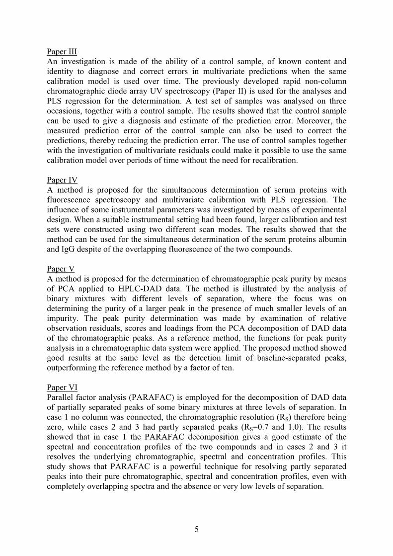
Paper III An investigation is made of the ability of a control sample, of known content and identity to diagnose and correct errors in multivariate predictions when the same calibration model is used over time. The previously developed rapid non-column chromatographic diode array UV spectroscopy (Paper II) is used for the analyses and PLS regression for the determination. A test set of samples was analysed on three occasions, together with a control sample. The results showed that the control sample can be used to give a diagnosis and estimate of the prediction error. Moreover, the measured prediction error of the control sample can also be used to correct the predictions, thereby reducing the prediction error. The use of control samples together with the investigation of multivariate residuals could make it possible to use the same calibration model over periods of time without the need for recalibration. Paper IV A method is proposed for the simultaneous determination of serum proteins with fluorescence spectroscopy and multivariate calibration with PLS regression. The influence of some instrumental parameters was investigated by means of experimental design. When a suitable instrumental setting had been found, larger calibration and test sets were constructed using two different scan modes. The results showed that the method can be used for the simultaneous determination of the serum proteins albumin and IgG despite of the overlapping fluorescence of the two compounds. Paper V A method is proposed for the determination of chromatographic peak purity by means of PCA applied to HPLC-DAD data. The method is illustrated by the analysis of binary mixtures with different levels of separation, where the focus was on determining the purity of a larger peak in the presence of much smaller levels of an impurity. The peak purity determination was made by examination of relative observation residuals, scores and loadings from the PCA decomposition of DAD data of the chromatographic peaks. As a reference method, the functions for peak purity analysis in a chromatographic data system were applied. The proposed method showed good results at the same level as the detection limit of baseline-separated peaks, outperforming the reference method by a factor of ten. Paper VI Parallel factor analysis (PARAFAC) is employed for the decomposition of DAD data of partially separated peaks of some binary mixtures at three levels of separation. In case 1 no column was connected, the chromatographic resolution (RS) therefore being zero, while cases 2 and 3 had partly separated peaks (RS=0.7 and 1.0). The results showed that in case 1 the PARAFAC decomposition gives a good estimate of the spectral and concentration profiles of the two compounds and in cases 2 and 3 it resolves the underlying chromatographic, spectral and concentration profiles. This study shows that PARAFAC is a powerful technique for resolving partly separated peaks into their pure chromatographic, spectral and concentration profiles, even with completely overlapping spectra and the absence or very low levels of separation.

2. Theory The theory section of this thesis comes under the main headings Spectroscopy, Liquid chromatography, Chemometrics, Experimental design and Multivariate data analysis. The text included under these headings refers to the analytical techniques and chemometric tools employed in the six papers discussed. 2.1 Spectroscopy Electromagnetic radiation is a type of energy that takes numerous forms, the electromagnetic spectrum encompassing a wide range of wavelengths and frequencies all the way from cosmic and gamma radiation (wavelength 10-14 to 10-12 m) to infrasonic radiation (1010 m) (Figure 2).

The termis resolvNowadayspectromwaves (analyticaRaman sSpectrosapplicati The are moleculeelectrom

U

6

Figure 2. Schematic description of the electromagnetic spectrum.

spectroscopy refers historically to processes where light or visible radiation ed into its component wavelengths in order to produce a spectrum.1 s, however, it is also used for other types of radiation such as ions (mass etry), the spin of nuclei (nuclear magnetic resonance spectroscopy), sound acoustic spectroscopy) etc. Some common spectroscopic techniques in l chemistry are UV-Vis spectroscopy, IR spectroscopy, NIR spectroscopy, pectroscopy, fluorescence spectroscopy and atomic absorption spectroscopy. copic techniques are of the utmost importance in analytical chemistry, with ons in a considerable number of fields.

process in which electromagnetic energy is transferred to the atoms or s of the sample is called absorption. Following absorption of the agnetic energy, atoms and molecules are excited to one or more higher energy

10-14 10-12 10-10 10-8 10-6 10-4 10-2 1 102 104 106 108

Cosm

ic radiation

Gam

ma radiation

X-ray radiation

Ultraviolet-visible radiation

Near Infrared radiation

Microw

ave radiationR

adar

Television

NM

R

Radio

1010

Ultrasonic

Sonic

Infrasonic

1015

Visible

Infrared

ltravioletWavelength (m)

Frequency (Hz)10101019

Infrared radiation

states, which exist at discrete levels. In order for the absorption of radiation to occur, the energy of an exciting photon must exactly match the energy difference between the ground state and one of the excited states. These energy differences are unique for each compound and a plot of the frequencies of absorbed radiation therefore provides a characterisation of a compound. An absorption spectrum with absorption plotted as a function of wavelength is thus very useful. The energy E associated with the absorption bands of a molecule is given by:

E = Eelectronic + Evibrational + Erotational (1) where Eelectronic describes the electronic energy of the molecule, Evibrational the vibrational energy and Erotational the rotation energy. The number of rotational levels in a molecule is much larger than the number of vibrational states and the number of vibrational states is in turn larger than the number of electronic levels. These facts are also related to the differences in energy among the different states, where:

Eelectronic > Evibrational > Erotational (2) Hence for a given molecule a number of electronic energy states exists, an even larger number of vibrational levels and also more rotational levels.

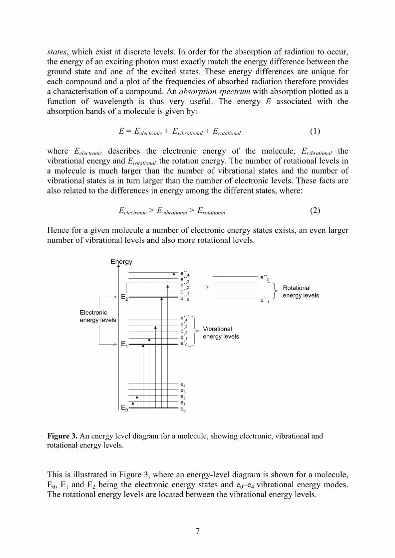
Figure 3rotationa This is iE0, E1 aThe rota

7

. An energy level diagram for a molecule, showing electronic, vibrational and l energy levels.

llustrated in Figure 3, where an energy-level diagram is shown for a molecule, nd E2 being the electronic energy states and e0–e4 vibrational energy modes. tional energy levels are located between the vibrational energy levels.

Energy

E0

E1

E2

e0

e1

e2

e3

e4

e´0

e´2

e´3

e´4

e´´0

e´´2

e´´3

e´´4

e´1

e´´1

Vibrational energy levels

Rotational energy levels

e´´1

e´´2

Electronic energy levels

When a beam of parallel radiation passes through a solution of a compound, absorption occurs (Figure 4). The radiant power before the beam has passed through the solution is P0 and after the passage through the solution is P. The thickness of the solution is b cm and the concentration c (g l-1).

Figure 4. Illustrati The fraction of intransmittance (T)

The logarithm of

The amount of ligabsorbance. Tran

while absorption directly proportioc, of the absorbin

where ε is the mosolutions having athere is no longer

b (cm)

8

on of the attenuation of a beam of radiation by an absorbing solution.

cident radiation that is transmitted by the solution is called the and is given by

T = P/P0 (3)

the transmittance is called the absorbance, A:

A= –log10 T (4)

ht absorbed can hence be expressed either as transmittance or as smittance is usually expressed as a percentage:

%T = 100(P/P0) (5)

is given by absorbance units (AU). The absorbance of a solution is nal to the path length, b, through the solution and the concentration, g species. This relationship is called the Lambert-Beer law:

A=ε*b*c (6)

lar absorptivity. A limitation of this law is that it is only linear for n absorbance of about <1.5 AU. Hence with too high a concentration

a linear relationship between the absorption and the concentration.

P0 (J) P (J)

c (g l-1)

9

2.1.1 Ultraviolet-visible absorption spectroscopy As Figure 2 shows, ultraviolet-visible (UV-Vis) radiation comprises only a small part of the electromagnetic spectrum (about 100–750 nm). Wavelength in UV-Visible absorption spectroscopy is generally denoted by the Greek letter lambda (λ) and usually stated in nano meters (nm). UV-Vis absorption spectroscopy can in simplified terms be described as the spectroscopy involving the electronic energy levels of a molecule, as shown in Figure 3. Hence the alternative name electronic spectroscopy is sometimes used since the absorption of radiation leads to transitions among the electronic energy levels of the molecule. When UV or visible radiation is absorbed by a molecular compound M, a two-step process occurs.1,2 First an electronic excitation takes place:

M + hν → M* (7) where hν represents the photon and M* is the electronically excited molecule. The excited state is very short-lived, however, due to relaxation processes and the molecule returns to its ground state in a very short time (10-8 to 10-9 s). The most common type of relaxation involves conversion of excitation energy to heat: M* → M + heat (8) The amount of thermal energy is, however, very low and not usually detectable. Hence the absorbance measurement does not generally disturb the system under investigation. Other types of relaxation involve fluorescent or phosphorescent re-emission. Two main types of electrons are involved in UV-Vis absorption spectroscopy of organic molecules, bonding and non-bonding. Bonding electrons participate directly in the formation of bonds between atoms, while the non-bonding electrons are unshared outer electrons not involved in any chemical bond, such as electrons in oxygen, nitrogen, sulphur and the halogens. The excitation of bonding electrons is generally the result of the absorption of UV-Vis radiation and hence some functional groups can be identified (chromophores). In addition, aromatic hydrocarbons in UV-Vis absorption spectroscopy generally show strong absorption. UV-visible absorption spectroscopy is thus normally sensitive to multiple bonds or aromatic conjunctions within molecules. In an organic molecule containing chromophores the electronic spectrum is often complex compared to that of a single atom. The explanation for this is that in the case of molecules the vibrational and rotational energy levels are superimposed on the electronic energy levels. This results in a broad band of absorption that often appears to be continuous. In Figure 5b a UV-Vis spectrum of lidocaine is shown. Some factors influencing the UV-Vis absorption spectrum of a sample are the solvent, pH and temperature. Generally the solvent should be transparent and not have an absorbance maxima intervening with the analyte. In addition, the polarity of the solvent can modify the electronic environment of the absorbing chromophore.3 Typical solvents used are water, ethanol or cyclohexane. Changes in pH can radically change the UV-Vis spectrum, although this can often be controlled by the use of a buffer, and

10

a thermostatted cell holder can be used to control the temperature if the sample analysed is affected by temperature. A spectrophotometer is an instrument for measuring the transmittance or absorbance of a sample as a function of the wavelength of electromagnetic radiation. The main components of a spectrophotometer used for transmittance or absorbance measurement are shown in Figure 5a.

Figure 5. a) Schematic drawing of the main parts of a spectrophotometer used for measuring absorbance or transmittance, b) example of a UV-Vis absorption spectrum (lidocaine). Firstly, a source of electromagnetic radiation is needed, the light source. In UV-visible absorption spectroscopy two types of light source are generally used, the deuterium lamp and the tungsten lamp. The deuterium lamp has a useful wavelength range of about 160–375 nm and the tungsten lamp a range of about 350–2500 nm. Most instruments are equipped with both a deuterium lamp covering the UV range and a tungsten lamp covering the visible range. The tungsten lamp has very long life and low noise, while the deuterium lamp has a limited life and the intensity of the light decreases over time. Some sort of dispersion device or wavelength selector is the next main component in a spectrophotometer used for absorbance measurement. The dispersion of visible light with a prism is an illustrative way to see how the visible light disperses into different wavelengths and colours. The use of prisms in modern spectrophotometers is, however, somewhat limited due to the fact that the dispersion with a prism is angularly non-linear and temperature-sensitive. In single wavelength detection interference or absorption filters can be used, although if it is necessary to vary the wavelength of the radiation continuously over a considerable range (scanning), some other technique is needed. In scanning spectrophotometers the wavelength selection is most often achieved with a grating. This consists of a hard, optically flat, polished, reflective surface onto which very narrow groves have been ruled. Light falling on the grating is reflected at different angles, depending on the wavelength. A monochromator is a device constructed for spectral scanning and it consists of an entrance slit, a collimating mirror producing a parallel beam of radiation, a dispersion device, a

a) b)

Source of electromagnetic radiation

Dispersion device

Sample compartment

Detector

UV-Vis Absorbance spectra of lidocaine

0

0.5

1

1.5

2

2.5

3

190 290 390 490 590

Wavelength (nm)A

bsor

banc

e

11

focusing element and an exit slit. The monochromator is not capable, however, of delivering totally monochromatic light; the output is instead a band of light. After the dispersion device the light reaches the sample in the sample compartment (Figure 5a). In UV-Vis absorption spectroscopy liquid samples are as a rule analysed in a cuvette. The cuvette is a rectangular-shaped sample cell with a given path length and volume. The sample cell used must be made of a material that passes radiation in the spectral region of interest, and in the UV-visible spectral range this is often quartz or fused silica. After the radiation passes the sample, it reaches the detector, which converts the light signal into an electrical signal. Ideally the detector should give a linear response over a wide range, with low noise and high sensitivity. The two most common types of detectors used in UV-Vis spectroscopy are a photomultiplier tube or a photodiode detector. The photomultiplier tube is basically a phototube capable of amplifying the signal for measurement of low radiant power. In a phototube the radiation causes the emission of electrons from a photosensitive solid surface. The photomultiplier tube contains additional surfaces that emit a cascade of electrons when struck by electrons from the photosensitive area. This type of detector yields good sensitivity over the entire UV-visible range and high sensitivity at low light levels. The photodiode detector is discussed in the next section. Besides the components described in Figure 5, a number of other optical components such as lenses and mirrors are also needed in a spectrophotometer. Various configurations of UV-Vis absorption spectrophotometers exist such as single- or dual -beam spectrophotometers.1-4 Both diode array spectrophotometers (described below) and conventional spectrophotometers are generally single-beam instruments. Dual-beam instruments generally have better stability since they compensate for changes in lamp intensity between measurements of sample and blank. They are, however, also more complicated with additional optical components that generally reduce sensitivity and sample throughput. The split-beam spectrophotometer is a variant of the dual-beam instrument that uses two detectors to analyse the sample and the blank simultaneously. The use of two independent detectors is, however, another potential source of drift.

12

2.1.2 Diode array detection When a semi conducting material such as SiO2 is exposed to light, it allows electrons to flow through it. The resistance of the semiconductor thus decreases when radiation is absorbed. The change in conductivity can be measured and the current obtained is proportional to the radiant power.3 This is the basic principle of the photodiode detector. If a capacitor is connected over a photodiode, it will be discharged when the incident light changes the conductivity of the semiconductor. The amount of charge needed to recharge the capacitor at regular intervals is proportional to the intensity of the light. The photodiodes can be arranged in arrays of numerous diodes. A diode array thus consists of a series of photodiode detectors positioned side by side. The individual photodiodes are part of an integrated circuit formed on a silicon chip. In this circuit each diode has a dedicated capacitor connected by a switch to a common output line and a shift register that controls the switches. The capacitors are initially charged to a specific level and when photons penetrate the semiconductor, the electrical charge generated discharges the capacitors. Recharging of the capacitors take place at regular intervals, the measuring period for each scanning cycle. The number of photons detected by each diode is proportional to the amount of charge needed to recharge the capacitors, which also is proportional to the light intensity. By measuring the variation in light intensity over the entire wavelength range, the absorbance spectrum is obtained. The number of diodes generally range from 6 to 4096, although 1024 detector elements are perhaps the most widely used.2,3 The difference between a conventional scanning UV-Vis spectrophotometer and a DAD spectrophotometer is shown in Figure 6. In the conventional UV-Vis spectrophotometer (Figure 6a) the polychromatic light of the source is focused on the entrance slit in the monochromator. The dispersion device in the monochromator then selectively transmits a narrow band of light. The light passes the exit slit and the sample, where absorption takes place and the transmitted light hits the detector. By measuring the intensity of the light reaching the detector of a blank sample and comparing it with the corresponding measurement of the sample, the absorbance of the sample is determined. Rotating the dispersion device allows different wavelengths to be analysed.

Figure 6. Schematic drawing of a) a conventional spectrophotometer and b) a diode array spectrophotometer.

Light source

Sample cell

Entrance slitDispersion device

Diode array

λ1 λ2 λnPolychromator

b)

Light source

Sample cell

Entrance slitDispersion device

Detector

Monochromator

λ1λn

a)

13

In Figure 6b the main parts of a diode array spectrophotometer are shown. The polychromatic light of the source first reaches the sample cell, where absorption occurs and the transmitted light is focused in the entrance slit. A major difference compared to the conventional spectrophotometer is that the monochromator is replaced by a polychromator. The dispersion device is thus placed after the sample cell and entrance slit and disperses the light into different wavelengths that hit the array of diodes. Each diode measures a narrow band of the spectrum and the size of the diode and entrance slit controls the bandwidth of light. The main advantages of diode array spectrophotometers are the very short time of analysis, excellent wavelength reproducibility and robustness.2 Conventional scanning UV-Vis spectrophotometers take longer to scan a spectrum than the diode array spectrophotometer, although the resolution is higher and the signal-to-noise ratio is lower. In this thesis UV-Vis absorption spectroscopy is used in five papers. In Paper I scanning UV-Vis spectroscopy and multivariate calibration are employed for qualitative and quantitative determinations. In Papers II and III the rapid diode array spectroscopy is used together with multivariate calibration for quantitative determination. In Papers V and VI HPLC-DAD data is analysed multivariate in order to determine chromatographic peak purity as well as to resolve the pure profiles of partly separated peaks.

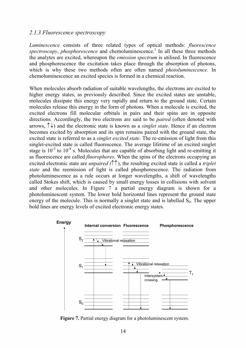
2.1.3 Fluorescence spectroscopy Luminescence consists of three related types of optical methods: fluorescence spectroscopy, phosphorescence and chemoluminescence.1 In all these three methods the analytes are excited, whereupon the emission spectrum is utilised. In fluorescence and phosphorescence the excitation takes place through the absorption of photons, which is why these two methods often are often named photoluminescence. In chemoluminescence an excited species is formed in a chemical reaction. When molecules absorb radiation of suitable wavelengths, the electrons are excited to higher energy states, as previously described. Since the excited states are unstable, molecules dissipate this energy very rapidly and return to the ground state. Certain molecules release this energy in the form of photons. When a molecule is excited, the excited electrons fill molecular orbitals in pairs and their spins are in opposite directions. Accordingly, the two electrons are said to be paired (often denoted with arrows, ↑↓) and the electronic state is known as a singlet state. Hence if an electron becomes excited by absorption and its spin remains paired with the ground state, the excited state is referred to as a singlet excited state. The re-emission of light from this singlet-excited state is called fluorescence. The average lifetime of an excited singlet stage is 10-5 to 10-8 s. Molecules that are capable of absorbing light and re-emitting it as fluorescence are called fluorophores. When the spins of the electrons occupying an excited electronic state are unpaired (↑↑), the resulting excited state is called a triplet state and the reemission of light is called phosphorescence. The radiation from photoluminescence as a rule occurs at longer wavelengths, a shift of wavelengths called Stokes shift, which is caused by small energy losses in collisions with solvent and other molecules. In Figure 7 a partial energy diagram is shown for a photoluminescent system. The lower bold horizontal lines represent the ground state energy of the molecule. This is normally a singlet state and is labelled S0. The upper bold lines are energy levels of excited electronic energy states.

Energy

14

Figure 7. Partial energy diagram for a photoluminescent system.

S0

S1

S2

Internal conversion Fluorescence Phosphorescence

Intersystem crossing

T1

Vibrational relaxation

Vibrational relaxation

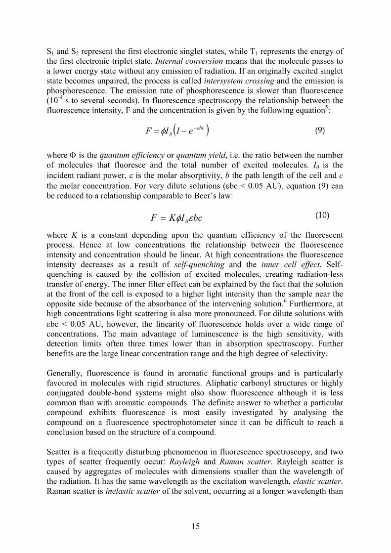
S1 and S2 represent the first electronic singlet states, while T1 represents the energy of the first electronic triplet state. Internal conversion means that the molecule passes to a lower energy state without any emission of radiation. If an originally excited singlet state becomes unpaired, the process is called intersystem crossing and the emission is phosphorescence. The emission rate of phosphorescence is slower than fluorescence (10-4 s to several seconds). In fluorescence spectroscopy the relationship between the fluorescence intensity, F and the concentration is given by the following equation5:

where Φ is the quantum eof molecules that fluoreincident radiant power, ε the molar concentration. be reduced to a relationsh

where K is a constant dprocess. Hence at low intensity and concentratiointensity decreases as a quenching is caused by transfer of energy. The inat the front of the cell is opposite side because of high concentrations light εbc < 0.05 AU, howeverconcentrations. The maindetection limits often thbenefits are the large linea Generally, fluorescence ifavoured in molecules wconjugated double-bond common than with aromacompound exhibits fluocompound on a fluoresceconclusion based on the st Scatter is a frequently distypes of scatter frequentlcaused by aggregates of the radiation. It has the saRaman scatter is inelastic

fficiency or quantum yield, i.e. the ratio between the number sce and the total number of excited molecules. I0 is the is the molar absorptivity, b the path length of the cell and c For very dilute solutions (εbc < 0.05 AU), equation (9) can ip comparable to Beer’s law:

epeconn sre

thenerexpthesca, th a

reer c

s fith systicresncruc

tury omome sca

( )bc0 e1IF εφ −−= (9)

15

nding upon the quantum efficiency of the fluorescent centrations the relationship between the fluorescence hould be linear. At high concentrations the fluorescence sult of self-quenching and the inner cell effect. Self- collision of excited molecules, creating radiation-less filter effect can be explained by the fact that the solution osed to a higher light intensity than the sample near the

absorbance of the intervening solution.6 Furthermore, at ttering is also more pronounced. For dilute solutions with e linearity of fluorescence holds over a wide range of

dvantage of luminescence is the high sensitivity, with times lower than in absorption spectroscopy. Further oncentration range and the high degree of selectivity.

ound in aromatic functional groups and is particularly rigid structures. Aliphatic carbonyl structures or highly tems might also show fluorescence although it is less compounds. The definite answer to whether a particular cence is most easily investigated by analysing the e spectrophotometer since it can be difficult to reach a ture of a compound.

bing phenomenon in fluorescence spectroscopy, and two ccur: Rayleigh and Raman scatter. Rayleigh scatter is

lecules with dimensions smaller than the wavelength of wavelength as the excitation wavelength, elastic scatter. tter of the solvent, occurring at a longer wavelength than

bcIKF 0εφ= (10)

16

the excitation, and originates from the abstraction of light energy by vibration modes of the solvent molecules. Instruments for measuring fluorescence contain the same basic components as UV-Vis spectrophotometers, namely a source of electromagnetic radiation, a wavelength selector, a sample cell, another wavelength selectors and a detector. In contrast to a UV-Vis spectrophotometer, two wavelengths selector or dispersion devices are needed, however, one for the excitation and one for the emission. The dispersion can be achieved with filters or with monochromators. Instruments using filters are generally called fluorometers, while instruments equipped with monochromators are called spectrofluorometers or fluorescence spectrophotometers since they provides both excitation and emission spectra.3 Figure 8 shows the basic components of a fluorescence spectrophotometer.

Figure 8. Schematic drawing of a fluorescence spectrophotometer.

Following the excitation, fluorescence is propagated from the sample in all directions. However, it is most convenient to measure it at a right angle to the excitation beam. The reason is that detecting the fluorescence intensity at other angles increases the scatter from the cell walls and from the solution. A scanning fluorescence spectrophotometer can measure in three different scan modes: excitation, emission and synchronous scan. In excitation scan the emission wavelength is fixed while the excitation wavelength is changed, thereby recording an excitation spectrum. Emission scan measures the emission at different wavelengths with the excitation wavelength fixed, which results in an emission spectrum. As previously mentioned, the emission always occurs at longer wavelengths than the excitation, due to small energy losses in the brief period before emission. By changing both the excitation and the emission wavelength in a stepwise manner, a synchronous scan can be performed. The interval between excitation and emission wavelengths is designated by the symbol delta (∆). Measuring synchronously with excitation at 250

Light source

Excitation monochromator

Sample Cuvette

Detector

Emissionmonochromator

Excitation

Emission

17

nm and with ∆λ=60 nm will then give the emission at 310 nm as the first point in the synchronous spectrum. If a whole emission spectrum is collected at each excitation wavelength, an excitation-emission matrix (EEM) can be constructed. The EEM thus consists of two-dimensional data, the fluorescence intensity as a function of excitation and emission wavelength. In Figure 9a the contour plot of an EEM for an analysis of albumin (Paper IV) is shown and the relative fluorescence intensity is depicted with different colours as function of the excitation and emission wavelengths. As can be seen, the fluorescence of albumin is in the lower left part of the EEM contour plot. Rayleigh and Raman scatter cause the diagonal bands shown. The vertical dotted line in Figure 9a shows the excitation scan collecting the emission at 340 nm and in Figure 9b the corresponding excitation spectrum is seen. The diagonal dotted line shows the synchronous scan ∆ 60 nm and the synchronous spectrum is shown in Figure 9c. The horizontal dotted line in Figure 9a shows the emission scan with an excitation of 280 nm and Figure 9d shows the corresponding emission spectrum. The principles of fluorescence spectroscopy have been further described elsewhere.5-9 Fluorescence spectroscopy is employed in this thesis in Paper IV for simultaneous multivariate determination of albumin and immunoglobuline G (IgG).

Figure 9. EEM and fluorescence spectra of albumin (20 µg ml-1): a) contour plot of EEM, b) excitation spectrum (emission at 340 nm recorded), c) synchronous spectrum (∆ 60 nm), d) emission spectrum (excitation at 280 nm).

-100

0

100

200

300

400

500

250 270 290 310 330 350 370 390

Excitation Wavelength (nm)

Excitation spectrum (Emission at 340 nm)

Fluo

resc

ence

Inte

nsity

-100

0

100

200

300

400

500

300 320 340 360 380 400 420 440

Emission Wavelength (nm)

Emission spectrum (Excitation at 280 nm)

Fluo

resc

ence

Inte

nsity

-100

0

100

200

300

400

310 330 350 370 390 410 430 450

Emission Wavelength (nm)

Synchronous scan ∆∆∆∆ 60 nm

Fluo

resc

ence

Inte

nsity

a) c)

b) d)

18

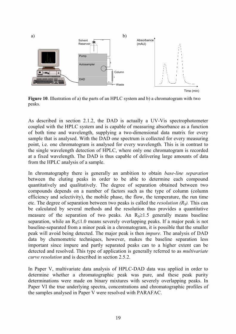
2.2 Liquid chromatography The word chromatography comes from the Greek words chroma meaning “colour” and graphein meaning “to write” and chromatography encompasses a diverse group of methods for the separation of compounds from each other. In all chromatographic separations the sample is dissolved in a mobile phase, which may be a gas or liquid that is then forced through a stationary phase. The components of the sample are distributed between the mobile and stationary phases in varying degrees and by elution of the mobile phase through the stationary phase separation of the compounds occurs. The most strongly retained components move slowly with the flow of the mobile phase, while fast-eluting compounds move rapidly with the mobile phase. If a detector that responds to the presence of the compounds is placed at the end and its signal is plotted as a function of time, a series of peaks is obtained, where each peak represents one compound. This is the outcome of a chromatographic analysis and it is called a chromatogram, consisting of a series of peaks over time. The time taken for different compounds to elute out of the stationary phase is generally called the retention time (Rt) and the height or area of the peaks in the chromatogram is related to the concentration of the compounds. In liquid chromatography (LC) the mobile phase consist of a liquid, while the stationary phase is generally a solid material fixed in a narrow steel tube, the column. In the early work on liquid chromatography highly polar stationary phases and relatively non-polar mobile phases were used. In modern liquid chromatography, however, the stationary phase is generally non-polar, while the mobile phase is polar, e.g. acetonitrile or methanol. To distinguish the two, the older type of chromatography is called normal-phase chromatography, while the newer type is called reversed-phase chromatography. In addition, in the early development of chromatography the particle size of the stationary phase was fairly large (>100 µm) and separation thus took a very long time. In the late 1960s. however, the technique of using smaller particle diameters (<10 µm) in the columns was developed and the name high-performance liquid chromatography (HPLC) was employed. When only a single mobile phase is used for the separation, we have isocratic elution, while when the composition of the mobile phase changes during the analysis, we have gradient elution. The instrumental parts of a modern HPLC system generally consist of a pump capable of delivering a constant flow of the mobile phase at a high pressure free from pulsation, an autosampler capable of injecting the samples in the flow of the mobile phase in a automatic and reproducible manner, and a detector of some kind. Detection with UV-Vis light is a very common detection method in HPLC using single or multiple wavelengths. Nowadays diode array detectors are often used instead of single wavelength detectors. The HPLC system is also often supplemented with a column oven, controlling the temperature of the column, and a computer with a chromatographic data system (CDS), which is used to control the HPLC system as well as to collect the data during the analysis. The parts of a modern HPLC system are illustrated in Figure 10a and an example of a chromatogram with two peaks is shown in Figure 10b.

19

Figure 10. Illustration of a) the parts of an HPLC systempeaks. As described in section 2.1.2, the DAD is actucoupled with the HPLC system and is capable of mof both time and wavelength, supplying a two-dsample that is analysed. With the DAD one spectrupoint, i.e. one chromatogram is analysed for everythe single wavelength detection of HPLC, where oat a fixed wavelength. The DAD is thus capable ofrom the HPLC analysis of a sample. In chromatography there is generally an ambitibetween the eluting peaks in order to be abquantitatively and qualitatively. The degree of compounds depends on a number of factors sucefficiency and selectivity), the mobile phase, the etc. The degree of separation between two peaks isbe calculated by several methods and the resolmeasure of the separation of two peaks. An separation, while an RS≤1.0 means severely overlabaseline-separated from a minor peak in a chromatopeak will avoid being detected. The major peak isdata by chemometric techniques, however, maimportant since impure and partly separated peadetected and resolved. This type of application is gcurve resolution and is described in section 2.5.2. In Paper V, multivariate data analysis of HPLC-determine whether a chromatographic peak wdeterminations were made on binary mixtures wPaper VI the true underlying spectra, concentratiothe samples analysed in Paper V were resolved with

Absorbance

DAD

Autosampler

Pump

Waste

Solvent Reservoir

Column

a) b)

and b) a chromatogram with two

ally a UV-Vis spectrophotometer easuring absorbance as a function

imensional data matrix for every m is collected for every measuring wavelength. This is in contrast to nly one chromatogram is recorded f delivering large amounts of data

on to obtain base-line separation le to determine each compound separation obtained between two h as the type of column (column flow, the temperature, the run time called the resolution (RS). This can ution thus provides a quantitative RS≥1.5 generally means baseline pping peaks. If a major peak is not gram, it is possible that the smaller

then impure. The analysis of DAD kes the baseline separation less ks can to a higher extent can be enerally referred to as multivariate

DAD data was applied in order to as pure, and these peak purity ith severely overlapping peaks. In ns and chromatographic profiles of PARAFAC.

Time (min)

(mAU)

20

2.3 Chemometrics As mentioned in the introduction chemometrics has emerged from chemistry and has introduced new methods capable of dealing with the large amounts of chemical data by means of multivariate data analysis. It also includes methods of performing experiments in a more rational and structured way by means of experimental design. The name chemometrics can be divided into chemo (from chemistry) and metric (meaning measurement). Chemometrics thus deals with chemical data and how to obtain information from it. One of the corner-stones of chemometrics is that data and information are not the same thing. As previously mentioned, data consists mainly of noise and information and the tools of chemometrics can be used to extract the information in the data. In chemometrics the extraction of information is performed by the use of a mathematical model. This model, however, can never describe a chemical system in detail, since it is always an approximation valid only in a limited interval. Moreover, models must always be validated before they are applied (discussed below). Another important aspect of chemometrics is that experiments should be performed in a structured manner, varying all the experimental variables at the same time, i.e. by using experimental design. All data should also be analysed simultaneously multivariate and not univariate since this approach generally gives more and deeper information. A final cornerstone of chemometrics is that its results are generally best illustrated graphically. People generally have difficulty looking at large data sets and drawing conclusions from the figures they contain. This can probably be explained by the fact that in the history of mankind we have always (until very recently) studied the world and reality surrounding us in the form of pictures. Human beings are thus probably more accustomed to discovering patterns in images than in large data sets since each figure in the data set is actually a symbol for a value that needs to be translated in our brain before we can understand it. The number of textbooks in the field is numerous.10-

19 To sum up, some of the cornerstones of chemometrics are:

• Data = information + noise • The model concept, i.e. models are always approximations and always

have to be validated • All variables should be changed and analysed simultaneously

(experimental design and multivariate data analysis) • Results are most easily investigated graphically

2.3.1 Dimensionality of analytical chemical data Analytical data can differ in its dimensionality, which restricts the types of chemometric method that can be applied to it. If the absorbance of a sample at a certain wavelength is measured with a UV-Vis spectrophotometer, the result is a single figure (Figure 11a). For instance, the absorbance at 245 nm of a sample containing a certain amount of lidocaine could be 0.32 absorbance units. If the absorbance of this sample were measured at more than one wavelength, the resulting data would be a one-dimensional array a spectrum. A wavelength range of 245–289 nm with a resolution of 1 nm would then result in a data array of 45 absorbance values. As described in section 2.2, the absorbance in HPLC-DAD is measured as a function of both wavelength and retention time. If it is measured at different retention times at a fixed wavelength, the resulting data is also a one-dimensional data array (Figure 11b), a chromatogram. If, however, the absorbance of a sample is measured as a function of both wavelength and retention time, the resulting data would be a two-dimensional matrix or table (Figure 11c). Hence if the sample containing a certain amount of lidocaine is analysed with HPLC-DAD, at 245–289 nm and a run time of 5 min with a frequency of 1Hz (1 spectrum collected each second), the resulting two-dimensional data would consist of 300*45 absorbance values. By analysing many samples, a three-way data set can be produced as a cube of data with three informative directions (Figure 11d). In the case of HPLC-DAD data, this means that the absorbance is expressed as a function of wavelength, retention time and samples.

a) b) c) d)One-dimensional Two-dimensional Three-dimensionalSingle figure

21

Figure 11. Illustration of a) single, b) one-, c) two- and d) three-dimensional data.

Wavelength

Tim

e

Sample

s

data data dataTwo-way data Three-way data One-way data

Tim

e

Wavelength

Tim

e

Absorbance as a function of both wavelengthand retention time.

Absorbance as a function of retention time at a fixed wavelength.

Absorbance as a function of wavelength, retention time and number of samples

Absorbance at a fixed wave-length and fixed retention time.

In addition, the response of an instrument from the analysis of one sample determines the order of the data. Data originating from hyphenated instruments like HPLC-DAD is called second-order data since it can be organised in a matrix.20 Another example of second-order data is the EEM in fluorescence spectroscopy. The resulting data from the analysis of a single sample on a UV-Vis spectrophotometer can be organised in a vector or a row and is therefore called first-order data. It should, thus be emphasised that second-order data is generally referred to as data, which can be arranged meaningfully in a matrix, like HPLC-DAD or EEM data. The analysis of a sample with two spectroscopic techniques like UV-Vis spectroscopy and IR spectroscopy does not produce second-order data since the UV and IR spectra cannot be meaningfully arranged in a matrix.20 It is important to note when discussing the shape of the data that one-dimensional data is generally illustrated in a two-dimensional plot, while two-dimensional data can be illustrated in a three-dimensional plot. This is shown in Figure 12, where the one-dimensional or first-order spectroscopic data array of the absorbance of lidocaine is plotted against wavelength (Figure 12a) and the absorbance as a function of wavelength and retention time in the DAD data for the same sample is shown (Figure 12b).

Figurone-diof two The dappliedefinidimenmost (PCAthat c

a) Absorbance (nm) (mA

U)

b)

22

e 12. Illustration of plots of data of different dimensionality: a) two-dimensional plot of mensional data, the absorbance as a function of wavelength, b) a three-dimensional plot -dimensional data, the absorbance as a function of wavelength and retention time.

imensionality of the data influences the kind of chemometric methods that can be d to it. No chemometric methods exist for one-dimensional data alone since by tion chemometrics is applied to multivariate data, meaning having more than one sion. If the first-order data of several samples is organised together in a table, the

common chemometric methods can be applied, i.e. principal component analysis )21,22, and partial least squares regression (PLS)23,24 etc. Multi-way data are data an be arranged according to more than two categories of variables and/or objects

Data :Wavelength (nm)

Wavelength (nm)

Time (min)

Data :Time (min)

Abso

r ban

ce

Wav

eleng

th(n

m)

23

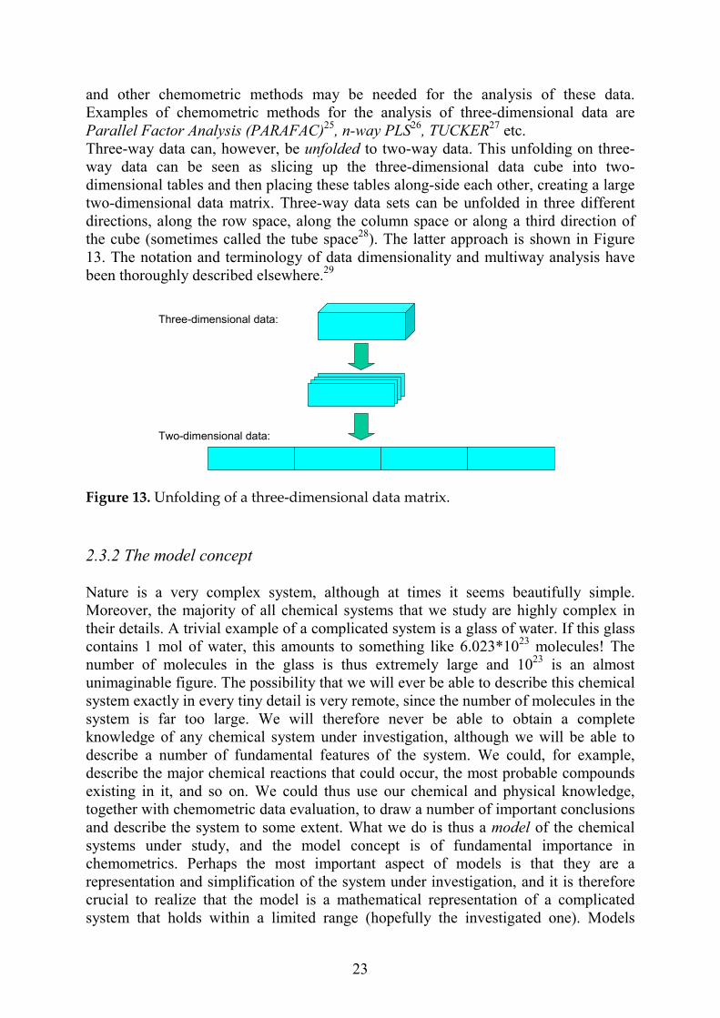
and other chemometric methods may be needed for the analysis of these data. Examples of chemometric methods for the analysis of three-dimensional data are Parallel Factor Analysis (PARAFAC)25, n-way PLS26, TUCKER27 etc. Three-way data can, however, be unfolded to two-way data. This unfolding on three-way data can be seen as slicing up the three-dimensional data cube into two- dimensional tables and then placing these tables along-side each other, creating a large two-dimensional data matrix. Three-way data sets can be unfolded in three different directions, along the row space, along the column space or along a third direction of the cube (sometimes called the tube space28). The latter approach is shown in Figure 13. The notation and terminology of data dimensionality and multiway analysis have been thoroughly described elsewhere.29 Figure 13. Unfolding of a three-dimensional data matrix. 2.3.2 The model concept Nature is a very complex system, although at times it seems beautifully simple. Moreover, the majority of all chemical systems that we study are highly complex in their details. A trivial example of a complicated system is a glass of water. If this glass contains 1 mol of water, this amounts to something like 6.023*1023 molecules! The number of molecules in the glass is thus extremely large and 1023 is an almost unimaginable figure. The possibility that we will ever be able to describe this chemical system exactly in every tiny detail is very remote, since the number of molecules in the system is far too large. We will therefore never be able to obtain a complete knowledge of any chemical system under investigation, although we will be able to describe a number of fundamental features of the system. We could, for example, describe the major chemical reactions that could occur, the most probable compounds existing in it, and so on. We could thus use our chemical and physical knowledge, together with chemometric data evaluation, to draw a number of important conclusions and describe the system to some extent. What we do is thus a model of the chemical systems under study, and the model concept is of fundamental importance in chemometrics. Perhaps the most important aspect of models is that they are a representation and simplification of the system under investigation, and it is therefore crucial to realize that the model is a mathematical representation of a complicated system that holds within a limited range (hopefully the investigated one). Models

Three-dimensional data:

Two-dimensional data:

always have to be validated in order to verify and ensure that they really hold true in the experimental domain investigated (discussed below). The model is thus a representation and simplification of the chemical system under investigation, describing important features of it. It is not possible to arrive at an exact description of the investigated system, although if we can come pretty close to doing this, we will have something very useful. 2.3.3 Validation As mentioned, validation is a crucial step of the model concept in chemometrics. Since it is always possible to make a mathematical model of any system at all, regardless of whether it only contains random variation, it is essential to always validate the model. The validation is needed in order to be able to decide whether or not the conclusions drawn from it are reliable, i.e. to make sure that the results can be extrapolated to new data. An unvalidated model is in principle useless since it is then possible that the conclusions drawn result only from random noise. Validation can be seen as testing the found model or map in the system or reality under investigation and thereby verifying that it holds true (Figure 14).

Figure 14. Validationactual conditions unde

Validation can be validation. Internal vthe model to validabeen previously usethat the best form ofrepresents the mostrecommended that oapply new data sets is further used. In iapplied and the discthis thesis. As menti

24

can be seen as verifying that the found model or map really holds in the r study.

divided into two main types: internal validation and external alidation means utilising the data that has been used to construct

te it, while external validation means that new data that not has d in the model is used for the validation. It goes without saying validation is external validation, since using completely new data objective way to validate a model. However, it is generally ne should first use an internal validation of the model and then and perform a thorough external validation of the model before it nternal validation a number of calculations and statistics can be ussion that follows applies to the chemometric methods used in oned in section 1, chemometric techniques are good at extracting

Model validation:

Map

Reality

25

information from large amounts of data. The variation in a data set can be described with variance which is given by the square of the standard deviation (s):

( )1n

xxs

n

1i

2

i

−

−=

∑= (11)

where x is the mean of the number of measurements n and xi is the individual values. The information content of a data matrix is closely connected to its variance. The term variation is, however, generally used in a broader sense than variance and it is not compensated for the number of degrees of freedom and is thus a less profound statistical term. When performing a multivariate data analysis on a set of data, the sum of squares of the total variance of the data set (SStotal) can be divided into two parts:

SStotal = SSmodel + SS residual (12) where SSmodel is the sum of squares of the variance explained by the model and SSresidual is the residual or unexplained variance. The aim of chemometric modelling is generally to capture the variance in a given data matrix in a simple model of low dimensionality. This means that the explained variance (SSmodel) should be as high as possible, leaving only a very small amount of unexplained variance (SSresidual). An important term in the internal validation of a model is therefore the explained variance:

Explained variance = (SStotal – SSresidual )/ SStotal (13) This measure is often called the goodness of fit18 or the model validation term and thus describes the amount of variance explained by a model. It is sometimes expressed as a percentage (100*eq 13). In order to obtain an estimate of the predictive ability of a regression model, a often used method is cross validation (CV).30 The basic principle of CV is as follows. In the used data set one sample is kept out of the calibration and a regression model is calculated from the remaining observations. The y value of the object taken away is then predicted with the calibration model constructed. The prediction error of this observation can then be calculated as the difference between the predicted and true value. This procedure is then repeated leaving out every sample in the calibration set once, the summed prediction error then indicating the predictive ability. This ‘leave one out’ cross validation is, however, generally valid only when the number of samples is small, for larger calibration sets, the procedure should be carried out by dividing the calibration set into smaller subgroups instead of single samples. By summing the prediction error sum of squares (PRESS)18 obtained in the cross validation:

PRESS = Σ (yobserved – ypredicted)2 (14) where yobserved is the true value and ypredicted is the predicted y value in the cross validation, a measure of the predictive ability of the model is given. By comparing

26

PRESS with the total sum of squares of the variance in the data set, the goodness of prediction measure can be calculated:

Goodness of prediction = (SStotal –PRESS) / SStotal (15)

A further important term in the internal validation is the decision of model dimensionality. This concerns the number of principal components (PCs, see section 2.5.3) that are used in the model. Generally the objective with the model is to explain as much of the variance in the data with as few PCs as possible in order to minimize the influence of noise and to obtain a simple model. Furthermore, a model consisting of too few components will result in under-fit, i.e. the model has not dealt with all the variance present in the data set. Correspondingly, a model with too many components will result in over-fit, since noise then is modelled to a higher extent. Over-fit also impairs the predictive ability of the model. This is illustrated in Figure 15 below. It is important, therefore, to find the optimum number of components to use in a model, and CV is a method often used for finding the optimal model dimensionality. Figure 15. Illustration of how the model dimensionality affects the fit and predictive ability. In the internal validation of a model the residuals are also used. The residuals are the difference between the actual and modelled values or, in other words, between the observed and predicted values. Plots of the residuals of a model will reveal outliers, trends etc. When using PCA or PLS for the data analysis, scores and loadings are also important measures in the internal model validation. These measures are further discussed in section 2.5.3 and 2.5.5. To sum up, important measures in the internal validation are: the explained variance, goodness of prediction, model dimensionality and an overview of the residuals, scores and loadings. In external validation new data not previously used in the model is applied in the validation. These sets of new samples are often called test sets. The samples in the test set should be well known, i.e. of known class and content. By comparing the predictions obtained with the true values of these samples, a good estimate of the predictive ability can be made and thereby validation of the calibration model (see also section 2.5.1) can be achieved.

Goodness of fit

Number of PC´s

Optimal model dimensionality

Over-fitUnder-fit

Amount explained or predicted variation

Goodness of prediction0

1

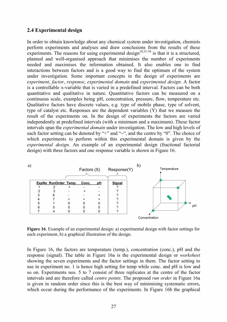
2.4 Experimental design In order to obtain knowledge about any chemical system under investigation, chemists perform experiments and analyses and draw conclusions from the results of these experiments. The reasons for using experimental design10,31-34 is that it is a structured, planned and well-organised approach that minimises the number of experiments needed and maximises the information obtained. It also enables one to find interactions between factors and is a good way to find the optimum of the system under investigation. Some important concepts in the design of experiments are experiment, factor, response, experimental domain and experimental design. A factor is a controllable x-variable that is varied in a predefined interval. Factors can be both quantitative and qualitative in nature. Quantitative factors can be measured on a continuous scale, examples being pH, concentration, pressure, flow, temperature etc. Qualitative factors have discrete values, e.g. type of mobile phase, type of solvent, type of catalyst etc. Responses are the dependent variables (Y) that we measure the result of the experiments on. In the design of experiments the factors are varied independently at predefined intervals (with a minimum and a maximum). These factor intervals span the experimental domain under investigation. The low and high levels of each factor setting can be denoted by “+” and “–“, and the centre by “0”. The choice of which experiments to perform within this experimental domain is given by the experimental design. An example of an experimental design (fractional factorial design) with three factors and one response variable is shown in Figure 16.

Fe Irsusiiw

TemperatureFactors (X) Response(Y)b)

a)

27

igure 16. Example of an experimental design: a) experimental design with factor settings for ach experiment, b) a graphical illustration of the design.

n Figure 16, the factors are temperature (temp.), concentration (conc.), pH and the esponse (signal). The table in Figure 16a is the experimental design or worksheet howing the seven experiments and the factor settings in them. The factor setting to se in experiment no. 1 is hence high setting for temp while conc. and pH is low and o on. Experiments nos. 5 to 7 consist of three replicates at the centre of the factor ntervals and are therefore called centre points. The proposed run order in Figure 16a s given in random order since this is the best way of minimising systematic errors, hich occur during the performance of the experiments. In Figure 16b the graphical

Concentration

pH

ExpNo RunOrder Temp. Conc. pH1 2 + - -2 3 - + -3 6 - - +4 7 + + +5 1 0 0 06 5 0 0 07 4 0 0 0

Signal???????

28

representation of the experimental design is shown, each factor having its own axis and each experiment being represented by a dot. The results of the experiments are used to calculate a regression model of the relationship between the factors (X) and the responses (Y) and polynomial approximations are generally used. Different types of model can be employed, but linear, interaction and quadratic models are most often used. An interaction model of the response Y to factors x1 and x2 consists of: Y=β0 + β1x1 + β2x2 + β12x1x2 + E (16) where β0 is the intercept, β1 the regression coefficient of the first factor (x1), β12 the regression coefficient of the interaction term describing the interaction between x1 and x2, and E the residual. The type of model required depends on the aim of the study. The linear and interaction model are generally sufficient for screening purposes, while optimisation requires quadratic terms. The types of regression involved in determining the model are generally multiple linear regression (MLR)16 or sometimes also PLS. If there are a large number of dependent factors or responses in the data set, it can be evaluated with PLS. Furthermore, if there is missing data in the data set or if the designs used are distorted, PLS can be applied to the data analysis. As previously mentioned, validation is a crucial step in chemometric modelling and the validation carried out in experimental design is very similar to that previously described. Some additional terms used in the validation of experimental designs are the significance of the regression coefficients and normal probability plots of the residuals. The replicated experiments of the centre points can be used to estimate the experimental error, which in turn in analysis of variance (ANOVA)19 can give an estimate of any lack of fit of the model. If an experimental design comprises too few experiments in relation to the number of factors under investigation, it can lead to confounding, i.e. the importance of the factors cannot be estimated independently of each other. The number of different experimental designs is many10, 31-34. One can divide the designs into two major groups based on the objective for which they are applied: screening and optimisation designs. The screening designs generally contain fewer experiments since their main objective is to sift important factors from non-important ones. The designs used for optimisation or response surface modelling (RSM) thus comprise more experiments since the aim is a deeper understanding of the experimental system under study. The optimisation designs generally vary each factor at more than three levels, while the screening designs often have each factor at only three levels. The fractional factorial designs form the basis of screening designs. Examples of experimental designs used for optimisation are the central composite designs, of which central composite circumscribed (CCC) is one of the most useful, having each factor at five levels. Different types of experimental design are described further elsewhere.31-34

29

When using experimental design in practice there are a few things that should be kept in mind in order to obtain good results, the main steps involved being shown in Figure 17. The first (and perhaps the most important step) is to stipulate clearly the aim of the investigation (Fig. 17a). Other important issues at this stage are determining what type of regression model to use and also defining the factors and responses and their interval. Since it is crucial where in the experimental domain the experiments are actually carried out, some effort should be made in regard to the decision about the factor interval. The consequence of variability is important here since too narrow a factor interval will result in a small variation in the resulting data and hence an unstable model. However, too large interval of the factors can also result in incorrect conclusions since one single factor may then dominate completely if its interval is too large. A final thing to do at this stage is to perform a few pre-trials to verify the chosen factor intervals. It is far better to discover whether any experiments are impossible to carry out for some reason at this stage than later on when working on a larger set of experiments in an experimental design.

Figure 17. Schematic description of the steps in using experimental design.

In the second step (Fig. 17b) the experimental design is constructed from the defined factors, responses and objective of the study. This is done with the help of some software for the actual experimental design. There is a large variety of computer software for constructing experimental designs and the data analysis of these. The choice of design follows mainly from the objective of the study. In the third step (Fig. 17c) the experiments are carried out in the laboratory according to the experimental design. If possible, they should be performed in random fashion in order to reduce the effect of errors such as differing day-to-day behaviour of the instrument or the analyst etc. When the experiments have been done and a measure of the response variable-(s) in every experiment has been obtained, the last step (Fig. 17d) concerns the data analysis, where the regression model is calculated and validated and the evaluation of the results takes place. Often the evaluation of the results leads to a new or refined aim of the study with new experiments, as illustrated by the dashed line in Figure 17. Experimental design was used in Paper II to investigate how three instrumental parameters as well as two ways of exporting a representative UV spectrum influenced predictive ability. In Paper IV experimental design was used to find a suitable instrumental parameter setting.

a) Establish the aim and initiate the study

b) Construct the experimental design

c) Perform the experiments

d) Data analysis and evaluation

2.5 Multivariate data analysis The term multivariate can be explained as “multi” meaning numerous or many and “variate” meaning variation or change. Multivariate data analysis is thus the analysis of data consisting of multiple variables measured from many samples. The aim of chemometric methods for data decomposition and reduction is to find a small number of latent variables that can explain all the variation in the data matrix studied. Multivariate data analysis thus tries to find the relationships between the variables and samples in the data set and capture them in new latent variables. Some important definitions in multivariate data analysis are the terms variables and observations, as shown in Figure 18 below. The rows of the matrix are generally called objects or observations and thus comprise the samples. The columns are in turn called variables and consist of the entities measured for each object. The variables are generally divided into X and Y. As previously mentioned, in experimental design the X variables are called factors, the y-variables responses and the objects experiments.

Figure 18. Illustrand responses. Multivariate mecalled regressionprincipal compomultivariate metrends, groups aanalogue to PCAOften differing analysis takes preduce the effecmodel (lower mTransformation distribution of ththe average of edata is said to deviation (s) fovariable by 1/s, called variance chemometric tex

Variables

30

ation of the terms objects, observations and experiments, variables, factors

thods that find the relationship between x and y-variables are generally methods, as previously mentioned. Examples of these methods are nent regression (PCR)16, PLS 23,24 and MLR16. Another example of a thod used for exploratory analysis and survey of the X data, finding nd outliers, is PCA.21,22 PARAFAC25 can in some sense be seen as the for three way data. pre-treatment of the data is carried out before the multivariate data lace. The reasons for performing data pre-treatment are generally to t of noise, improve the predictive ability of the model and simplify the odel dimensionality) by making the data more normally distributed. is pre-treatment by means of a mathematical formula to change the e data, examples being logarithmic and exponential transformation. If ach variable is calculated and then subtracted from the variables, the be mean-centred. Unit variance scaling means that the standard

r each variable is calculated and by multiplying each value of that all variables are then given an equal weight. This is also sometimes scaling. Further examples of pre-treatment are described elsewhere in tbooks.10-18

X YObjects, observationsor experiments

Factors Responses

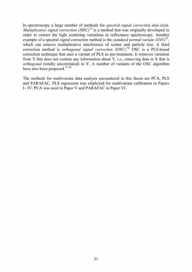
31

In spectroscopy a large number of methods for spectral signal correction also exist. Multiplicative signal correction (MSC)15 is a method that was originally developed in order to correct the light scattering variations in reflectance spectroscopy. Another example of a spectral signal correction method is the standard normal variate (SNV)35, which can remove multiplicative interference of scatter and particle size. A third correction method is orthogonal signal correction (OSC).36 OSC is a PLS-based correction technique that uses a variant of PLS as pre-treatment. It removes variation from X that does not contain any information about Y, i.e., removing data in X that is orthogonal (totally uncorrelated) to Y. A number of variants of the OSC algorithm have also been proposed.37,38 The methods for multivariate data analysis encountered in this thesis are PCA, PLS and PARAFAC. PLS regression was employed for multivariate calibration in Papers I– IV. PCA was used in Paper V and PARAFAC in Paper VI.

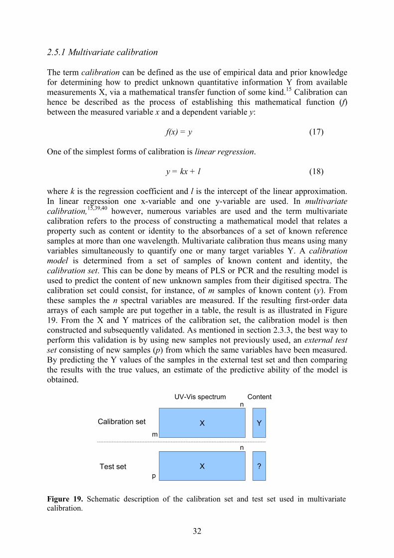
2.5.1 Multivariate calibration The term calibration can be defined as the use of empirical data and prior knowledge for determining how to predict unknown quantitative information Y from available measurements X, via a mathematical transfer function of some kind.15 Calibration can hence be described as the process of establishing this mathematical function (f) between the measured variable x and a dependent variable y:

f(x) = y (17) One of the simplest forms of calibration is linear regression. y = kx + l (18) where k is the regression coefficient and l is the intercept of the linear approximation. In linear regression one x-variable and one y-variable are used. In multivariate calibration,15,39,40 however, numerous variables are used and the term multivariate calibration refers to the process of constructing a mathematical model that relates a property such as content or identity to the absorbances of a set of known reference samples at more than one wavelength. Multivariate calibration thus means using many variables simultaneously to quantify one or many target variables Y. A calibration model is determined from a set of samples of known content and identity, the calibration set. This can be done by means of PLS or PCR and the resulting model is used to predict the content of new unknown samples from their digitised spectra. The calibration set could consist, for instance, of m samples of known content (y). From these samples the n spectral variables are measured. If the resulting first-order data arrays of each sample are put together in a table, the result is as illustrated in Figure 19. From the X and Y matrices of the calibration set, the calibration model is then constructed and subsequently validated. As mentioned in section 2.3.3, the best way to perform this validation is by using new samples not previously used, an external test set consisting of new samples (p) from which the same variables have been measured. By predicting the Y values of the samples in the external test set and then comparing the results with the true values, an estimate of the predictive ability of the model is obtained. Figure 19. Sccalibration.

UV-Vis spectrum Content

32

hematic description of the calibration set and test set used in multivariate

X YCalibration set

X ?Test set

m

n

n

p

There are a number of reasons for using multivariate calibration. Univariate calibration works well as long as no other compounds in the solution analysed absorb light at the wavelength used, i.e. the wavelength is selective for the compound under study. If this is not the case, all the other absorbing compounds, i.e. the interferences in the solution must be known. In multivariate calibration, however, this is not the case since using many x-variables automatically corrects for each other’s selectivity problem, and the x-variables used thus do not need to be totally selective. The precision of multivariate calibration is generally high as long as there is a linear relationship between the x and y-variables. Multivariate calibration is also generally more robust to small changes in the experimental or instrumental parameters such as small changes in pH, temperature or lamp intensity. Samples that differ in some way, outliers, are also more easily spotted and evaluated with multivariate data than with univariate data since multivariate residuals will show how an unknown sample fits into the calibration model. In addition, in multivariate calibration numerous graphical diagnostic tools are generally available. The calibration samples should in the calibration set span the calibration experimental domain as far as possible and experimental design can be used to find suitable samples to include in the calibration set. Also the best calibration is generally obtained when the calibration model contains all the sources of variation that can occur in the actual measurement. The order in which the samples are analysed is one source of variation and randomisation of the order of analysis minimises the error caused by day-to-day variations. The evaluation of the predictive ability of a quantitative multivariate calibration model can be made, by means of the root mean square error of prediction (RMSEP)15 and relative standard error of prediction (RSEP).41,42

where ypred is the predreference value of the cothe test set. RMSEP givinitial data, while RSEPpercentage. RSEP has alof the concentrations.42 Iwell established and stan

RSEP

)p(

)yy(RMSEP

2obspred

p

1i

−

=∑

=

(19)

33

icted concentration in the sample, yobs is the observed or ncentration in the sample and p is the number of samples in

es an estimate of the prediction error in the same unit as the gives a relative measure of the prediction error in terms of so been defined as the relative standard deviation of residuals n recent years the use of multivariate calibration has become dardised guidelines have been published.43

2obs

2obspred

p

1i

)y(

)yy(*100(%)

∑

∑ −= =

(20)

34

A general problem in multivariate calibration is the issues surrounding calibration transfer.44 When a multivariate calibration model is constructed on one occasion and used for the prediction of samples on later occasions or in samples analysed on other instruments, there is always some influence from small variations in the instrumental parameters. This variation can lead to errors in the predictions obtained, and a number of chemometric methods have been applied to this problem.44-49 In Paper III a way of detecting and correcting bad predictions in multivariate calibration is presented, i.e. by using control samples. Multivariate calibration is also applied in Papers I, II and IV. 2.5.2 Multivariate curve resolution In analytical chemistry there is generally a wish to determine all the compounds present in mixtures, ultimately by both quantifying and characterising them. In a mixture of three compounds analysed by some kind of spectroscopic technique, this would mean obtaining both the quantity and pure spectra of these three compounds. As previously described, spectroscopic instruments can deliver large amounts of data in a very short period of time, and this fact is utilised in many coupled or hyphenated50 analytical techniques like LC-DAD and LC-MS. The resulting data are of second-order and if this data is analysed with chemometric techniques, quantification and characterisation can take place. The chemometric applications that try without any calibration or standard samples to obtain the pure profiles (i.e. chromatograms, spectra and concentrations) of the compounds in mixtures are generally called multivariate curve resolution or self-modelling curve resolution. A large number of methods have been proposed for both two-way data51-59 as well as for data of higher dimensionality.60,61,26 Further descriptions of methods for curve resolution can be found elsewhere.62 As previously mentioned, a general ambition in chromatography is to obtain baseline-separated or “complete” separated peaks. The reason for this is the tradition of using univariate calibration, i.e. to correlate the peak area obtained by detection at a single wavelength with the concentration of each compound. If, however, multivariate data is used, partly separated peaks are generally sufficient for quantification as long as the compounds analysed to some extent have different UV-Vis spectra. Furthermore, with partial separation large time savings are obtained since the run time of the chromatograms can be substantially reduced. In this thesis PCA is employed in Paper V to determine the chromatographic peak purity of partly separated peaks. In this paper Evolving Factor Analysis (EFA) is also employed for comparison with the PCA method proposed. PARAFAC is used in Paper VI to resolve the pure chromatographic, spectral and concentration profiles of unresolved chromatograms.

2.5.3 Principal component analysis In the following text capital boldface letters (X) represent two-way matrices, underlined capital bold face letters (X) three way arrays and lower-case boldface letters (x) vectors (one-way arrays). PCA is a well-known chemometric method for the decomposition of two-way matrices.21,22 The variance in the data matrix X, with m observations and n variables, is decomposed by successively estimating principal components (PCs) that capture the variance in the data in scores and loadings. In Figure 20 the geometrical interpretation of PCA on a small data set consisting of twelve observations and three variables is shown. The steps in the geometrical interpretation of PCA are as follows. Firstly the X-space is given a coordinate system where each variable gets an axis whose length corresponds to its scaling. In this example three variables mean three coordinate axes. Each observation in this space is represented by a point. The average of each variable is then calculated and subtracted (mean centring). This is equivalent to moving the swarm of points to the centre of the coordinate system. Thereafter a function is fitted to the data that describes as closely as possible the variance of the observations in the X-space. This is the first PC and is represented by the line in Figure 20b.

Figure 20. Geometrical interpretation of a Pconsisting of twelve objects and three variabcalculated from the data set. By projecting each point down to the distance between the centre point and thobservation is obtained. Since the data seof score values (t1) are obtained for the variable axis determines the influence loading value is given for each variablescore values and three loading values arehas been calculated, the remaining unexE:

X= TP The decomposition of a matrix with Pwhere the initial data matrix X is decomp

a) b)123456789101112

x1 x2 x3

X

35

CA model consisting of one PC: a) data set les, b) a geometric interpretation of the first PC

line (Euclidian distance) and measuring the e projection point, the score value (t) of each t consists of twelve objects, the same number

first PC. The angle between the line and each of each variable, the loading value (p). One in the data set (p1). In this example twelve thus given for the first PC. When the first PC plained variance is left in the residual matrix,

´ + E (21)

CA is schematically described in Figure 21, osed with PCA using two PCs.

x1

t1

x2

x3

x1

36

Figure 21. Schematic description of a decomposition of a matrix X with PCA using two PCs. After the first PC has been calculated, the next is calculated on the residual matrix E1, which contains the variance not explained by the first PC.

X = t1p1´+ t2p2´+ … + tapa´ + E (22)

The second PC is orthogonal to the first. More PCs (a) can be calculated as long as unexplained information is left. The significant number of principal components can be estimated by different methods, of which cross validation is an often-used method. The variance of a principal component is described by the eigenvalue, which is proportional to the variance explained by a PC. The eigenvalue (λ) can be described as the length of the PC and estimated as the sum of squares of the scores:

where tma is the score of object m for component a. Hence the length of the score vector is proportional to the importance of the particular PC describing how much of the variance in X that is explained. Although PCA can be calculated using different algorithms, the two methods most common are non-linear iterative partial least squares (NIPALS)22 and singular value decomposition (SVD).21 One problem with applying PCA to matrices with a chemical rank larger than one is that is does not give directly interpretable profiles like chromatograms and spectra since scores and loadings become linear combinations of the true analytical profiles. This issue is also called the problem of rotational freedom since the scores and loadings can be rotated without changing the fit of the model. In this thesis PCA was used for the analysis of chromatographic peak purity in Paper IV.

(23)

= +X t1

p1´

E1

PC1

E1 = t2

p2´

E2+

PC2

∑=

=M

1m

2matλ

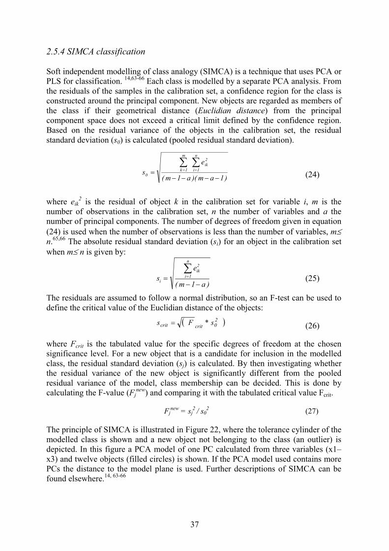
2.5.4 SIMCA classification Soft independent modelling of class analogy (SIMCA) is a technique that uses PCA or PLS for classification. 14,63-66 Each class is modelled by a separate PCA analysis. From the residuals of the samples in the calibration set, a confidence region for the class is constructed around the principal component. New objects are regarded as members of the class if their geometrical distance (Euclidian distance) from the principal component space does not exceed a critical limit defined by the confidence region. Based on the residual variance of the objects in the calibration set, the residual standard deviation (s0) is calculated (pooled residual standard deviation). where eik

2 is the residual number of observations innumber of principal compo(24) is used when the numn.65,66 The absolute residuawhen m≤ n is given by: The residuals are assumeddefine the critical value of where Fcrit is the tabulatedsignificance level. For a nclass, the residual standardthe residual variance of tresidual variance of the mcalculating the F-value (Fj

n

The principle of SIMCA ismodelled class is shown adepicted. In this figure a Px3) and twelve objects (filPCs the distance to the mfound elsewhere.14, 63-66

(24)

of object k in the calibration set for variable i, m is the the calibration set, n the number of variables and a the nents. The number of degrees of freedom given in equation

ber of observations is less than the number of variables, m≤ l standard deviation (si) for an object in the calibration set

to fthe E

vaew o devhe nodeew) a

illund aCA

led codel

)1am)(a1m(

es

n

1i

2ik

m

1k0 −−−−

=∑∑

==

(25)

ollow a normal distribution, so an F-test can be used to uclidian distance of the objects:

)a1m(

es

n

1i

2ik

i −−=

∑=

37

(26)

lue for the specific degrees of freedom at the chosen bject that is a candidate for inclusion in the modelled iation (sj) is calculated. By then investigating whether ew object is significantly different from the pooled l, class membership can be decided. This is done by nd comparing it with the tabulated critical value Fcrit.

Fjnew = sj

2 / s02 (27)

strated in Figure 22, where the tolerance cylinder of the new object not belonging to the class (an outlier) is

model of one PC calculated from three variables (x1–ircles) is shown. If the PCA model used contains more plane is used. Further descriptions of SIMCA can be

( )20critcrit s*Fs =

38

Figure 22. Illustration of the tolerance cylinder in SIMCA classification.

SIMCA was applied for the determination of identity in Paper I. In Paper III SIMCA was suggested as a way of identifying poor predictions and together with the use of control samples thereby making it possible to use the same multivariate calibration model over time without the need for recalibration.

PC

Critical limit

ResidualOutlier

Tolerance Cylinder

x1

x3

x2

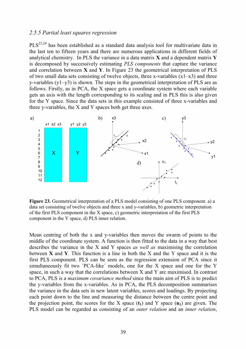
39

2.5.5 Partial least squares regression PLS23,24 has been established as a standard data analysis tool for multivariate data in the last ten to fifteen years and there are numerous applications in different fields of analytical chemistry. In PLS the variance in a data matrix X and a dependent matrix Y is decomposed by successively estimating PLS components that capture the variance and correlation between X and Y. In Figure 23 the geometrical interpretation of PLS of two small data sets consisting of twelve objects, three x-variables (x1–x3) and three y-variables (y1–y3) is shown. The steps in the geometrical interpretation of PLS are as follows. Firstly, as in PCA, the X space gets a coordinate system where each variable gets an axis with the length corresponding to its scaling and in PLS this is also given for the Y space. Since the data sets in this example consisted of three x-variables and three y-variables, the X and Y spaces both get three axes.

Figure 23. Geometrical interpretation of a PLS model consisting of one PLS component. a) a data set consisting of twelve objects and three x and y-variables, b) geometric interpretation of the first PLS component in the X space, c) geometric interpretation of the first PLS component in the Y space, d) PLS inner relation. Mean centring of both the x and y-variables then moves the swarm of points to the middle of the coordinate system. A function is then fitted to the data in a way that best describes the variance in the X and Y spaces as well as maximising the correlation between X and Y. This function is a line in both the X and the Y space and it is the first PLS component. PLS can be seen as the regression extension of PCA since it simultaneously fit two ´PCA-like´ models, one for the X space and one for the Y space, in such a way that the correlations between X and Y are maximised. In contrast to PCA, PLS is a maximum covariance method since the main aim of PLS is to predict the y-variables from the x-variables. As in PCA, the PLS decomposition summarises the variance in the data sets in new latent variables, scores and loadings. By projecting each point down to the line and measuring the distance between the centre point and the projection point, the scores for the X space (t1) and Y space (u1) are given. The PLS model can be regarded as consisting of an outer relation and an inner relation,

a)

123456789101112

x1 x2 x3

Y

y1 y2 y3

X

x1y1

t1 u1

u1

t1

x3

x2 y2

y3c) b)

d)

40

where the outer relation describes the X and Y block individually, while the inner relation links the two blocks together.23 The outer relations is given by

X = TP´+ E (28)

Y= UC´+ F (29)

where T is the score matrix and P´ the loading matrix of the X space, U the score matrix and C´ the loading matrix of the Y space. E and F are the residual matrices of the X and Y spaces respectively. By plotting the t1 values of the twelve objects in the example in Figure 29 against the corresponding u1 values, the PLS inner relation showing the correlation structure between X and Y is obtained (Figure 23d).

U=BT+H (30) where B is an identity matrix and H is a residual matrix. In PLS a type of additional loadings is calculated that expresses the correlation between X and Y, the weights, W. The weights are related to the PLS regression coefficients, BPLS: BPLS=W(P´W)-1C´ (31) The regression coefficients show the direction and magnitude of the influence of an x-variable on a specific y-variable. The prediction of y-variables of new samples is given by

Y=XBPLS + F (32) After the first PLS component has been calculated the next one can be calculated on residual matrices E and F. The number of significant PLS components (the model dimensionality) in a calibration model can be decided by means of cross validation. The matrices in PLS regression are shown schematically in Figure 24 and, for each new PLS component, t, u, w, p and c are calculated. The details of PLS regression have been thoroughly described elsewhere.23,24

Figure 24. Schematic description of the matrices in PLS regression.

T Uscores Y

Raw data

X

Raw data

E

residuals X

F

residuals Y

W´ weights

P´ loadings C´loadings

2.5.6 Parallel factor analysis Parallel factor analysis (PARAFAC) is a decomposition method for three-way arrays (or higher) that can be seen as a generalisation of bilinear PCA to higher order arrays.25 The original algorithms were developed by psychometricians for the decomposition of multiblock data.67-71 In PARAFAC each component is trilinear, in contrast to bilinear PCA, where one score and one loading vector are obtained for each component. For a I*J*K matrix three loading vectors (aif, bjf, ckf) are therefore given for each PARAFAC component (F). The PARAFAC model of a three-way array is found by minimising the sum of the squares of the residuals eijk

The decomposition of a described in Figure 25.

Figure 25. Schematic descriptPARAFAC. Two components Each PARAFAC componenprofile (af), one related to thsamples (cf). Hence one loaleast squares (ALS) can bspecial feature of PARAFAunique, which means that thobtained with PARAFAC PARAFAC algorithm is ncalculated simultaneously festimate of the number of Pthe initial PARAFAC algocause departures of tri-linPARAFAC was employed partly separated peaks into t

X

WavelengthTime

Samples

41

three-way array of HPLC-DAD data is schematically

ion of the decomposition of a three-way matrix X with are calculated.

t gives three loadings: one related to the chromatographic e spectral profile (bf) and one related to the content of the ding is given for each dimension in the data. Alternating

e used to find the solution to the PARAFAC model. A C compared to PCA is that the solutions obtained are

ere is no rotational problem as in PCA. Hence the loadings can be directly interpreted chemically. Furthermore, the ot sequential as in PCA since the tri-linear model is

or all components. One drawback of PARAFAC is that an ARAFAC components is needed in advance. A variant of

rithm that can handle shifts in retention time (which can earity) has also been proposed, called PARAFAC2.72,73 in Paper VI for the decomposition of HPLC-DAD data of he pure profiles.

ijkkfjf

F

1fifijk ecbax += ∑

=

= + + E

c1

b1

a2a1

b2

c2

(33)

42

3. Discussion In the following section discussion of the six papers in this thesis takes place. The aim has been to place the papers presented in context to some extent against what has previously been reported in the literature and to discuss important aspects such as advantages and drawbacks as well as sources of error. 3.1 Paper I Applications of UV-Vis spectroscopy and multivariate calibration are less often seen in the literature than applications involving vibrational spectroscopy (NIR, IR and Raman); although quantitative multivariate determinations using UV-Vis spectroscopy have been reported previously, qualitative determinations with classification are very rare. One explanation for this might be that the UV-Vis spectra of organic compounds are perhaps seen as less informative. The text book by Skoog and Leary puts it as follows “Ultraviolet and visible spectrophotometry have somewhat limited application for qualitative analysis, because the number of absorption maxima and minima is relatively small. Thus unambiguous identification is frequently impossible1.” UV-Vis spectroscopy has, however, been used for quantitative analysis with multivariate data analysis in a number of studies74-83, although the author has not previously seen qualitative analysis with SIMCA classification applied to UV-Vis data. In Paper I a method is proposed for the determination of the content and identity of the active compound in pharmaceutical solutions by means of UV-Vis spectroscopy and multivariate calibration. The determination of content is done by PLS regression and the identification with SIMCA classification. The study illustrates how the same calibration model can be used for obtaining both quantitative and qualitative information and how very similar and seemingly identical UV spectra can be distinguished using multivariate data analysis. In the following discussion the method proposed in Paper I is denoted the UV method. As shown in Paper I, the accuracy, precision and repeatability with the UV method were comparable or even slightly better than the HPLC reference method. The determination of the identity using SIMCA was also successful even though the UV spectra of lidocaine, bupivacaine, ropivacaine and mepivacaine are very similar. All six compounds used in the study had absorbances in the wavelength region 245–290 nm. In Paper I an empirical classification limit was used instead of the critical limit given by the software. The reason for using this empirical classification limit was that the critical limit proposed by the software in some previous cases using spectroscopic data was shown to be less appropriate. This is probably related to the fact that the software manufacturer has tried to set a very general critical limit that should be applicable in many different cases. The empirical classification limit used in Paper I was, however, also, narrower, in fact, than the limit proposed by the software.

43

The explanation of the spectral differences making possible the classification of the very similar UV spectra is illustrated in Figure 26, where the results of a classification of two samples are shown. The first sample in Figure 26 contained bupivacaine (0.20 mg ml-1) and it obtained a negative identity, while the other sample containing lidocaine (0.095 mg ml-1) got a positive identity.

Figure 26. Illustration of the small spectral diffein Paper I: a) contribution plot of a sample comparison of UV spectrum of the bupivacainlidocaine samples in the calibration set, c) contricontaining lidocaine (0.095 mg ml-1), d) UV spethe average calibration spectrum. In Figure 26a the contribution plot of a samcan be seen the contributing variables that gthe range 245–275 nm. Figure 26b shows thbupivacaine sample and the average specalibration set. In this figure the two spectrathe average spectrum has been multiplied bythe shape of the two spectra. The two specarefully investigating the spectra, a numberindicated in Figure 26b with arrows. The lo

245 250 255 260 265 270 275 280 285 290

Wavelength (nm)

Bupivacaine (0.20 mg/ml) Average Lidocaine spectra

-0.20

-0.10

0.00

0.10

0.20

245 250 255 260 265 270 275 280 285 290

DM

odX

Con

tribP

S[1

](38)

, Wei

ght=

VIP

1

Var ID (Primary)

a)

c)

-0.20

-0.10

0.00

0.10

0.20

245 250 255 260 265 270 275 280 285 290D

Mod

XC

ontri

bPS

[1](2

9), W

eigh

t=V

IP1

Var ID (Primary)

d)

b)

rences captured by the SIMCA classification containing bupivacaine (0.20 mg ml-1), b) e sample and the average spectrum of the

bution plot of a sample in the external test set ctrum of the lidocaine sample compared with

ple containing bupivacaine is shown. As ive this sample a negative identity are in e comparison of the UV spectrum of the

ctrum of the lidocaine samples in the have been normalised to each other, i.e. a constant in order to be able to compare ctra are overlaid and, as can be seen by of differences appear, some of which are cal minimum around 255 nm is slightly

245 250 255 260 265 270 275 280 285 290

Wavelength (nm)

Lidocaine (0.095 mg/ml) Average Lidocaine spectra

44

different in the two spectra. In the case of the bupivacaine sample it is located at 256 nm while for lidocaine it is at 254.4 nm. The bupivacaine spectrum also has a slightly different shape around 260 and 265 nm and the local minimum at about 270 nm for bupivacaine is 269.8 nm while for lidocaine it is 269.6 nm. Also the local maximum around 271 nm is slightly different between lidocaine and bupivacaine. In addition, the slopes of the two spectra differ in some wavelength regions: 256–260, 263–267 and 267–269 nm. There are thus a number of spectral differences between the UV absorption spectra of bupivacaine and lidocaine, which is what makes the SIMCA classification work. In Figure 26c the contribution plot of a sample containing only lidocaine is shown and, as can be seen, there are only very small random contributions from the different variables. In Figure 26d the corresponding spectrum of the lidocaine sample is compared with the average calibration spectrum and the fit of the two spectra is almost perfect. In fact, it is possible by multiplication by a constant integer to make a perfect overlay of any of the lidocaine spectra in the external test set on the average calibration spectrum. This is something that is impossible with the UV spectra of for instance bupivacaine, ropivacaine and mepivacaine. A source of systematic error was the fluctuations in the energy of the deuterium UV-lamp in the spectrophotometer, and this drift in the lamp occurred in spite of the double-beam instrument. The SIMCA classification did, however, recognise whether the UV spectra of lidocaine samples differed significantly and this was, in fact, the reason why the initial problems of drift in the lamp energy were discovered. This is an example, therefore, of how multivariate residuals can diagnose outlying samples. The OSC correction, together with the randomisation of the scan order, was, however, able to remove the small changes in the spectrum that this drift caused. An investigation of the OSC loadings (not shown here) revealed that the OSC removed small random variation at all wavelengths, which is what would have been expected from random noise caused by drift in the lamp intensity. For this type of errors, OSC is a good remedy since it removes portions of the X data that are linearly unrelated to the response. Furthermore, the randomisation of the order of analysis or scanning is important. Another possible source of error in the method proposed might be small differences in the sample cells used, something which, however, can be controlled by the use of matched cuvettes. An error in the text of Paper I is the cause of the shape of the UV spectrum of lidocaine in the wavelength range 190–210 nm. The shape of the spectrum in this wavelength range is most likely caused by the solvent (water) and not to the presence of stray light mentioned in the paper. The lower wavelength limit (UV cut off) for water is about 205 nm; below this limit water shows excessive absorbance and sample absorbance is not recorded linearly. The classification using the data in Paper I (test set B) have also been carried out for the same data, but with reduced spectral resolution (1 nm) as well as without the OSC correction, and the results were in principle the same as reported in Paper I. The only minor differences regarding the classification results were that some calibration samples got slightly higher sj values and there was a slight decrease in the differences

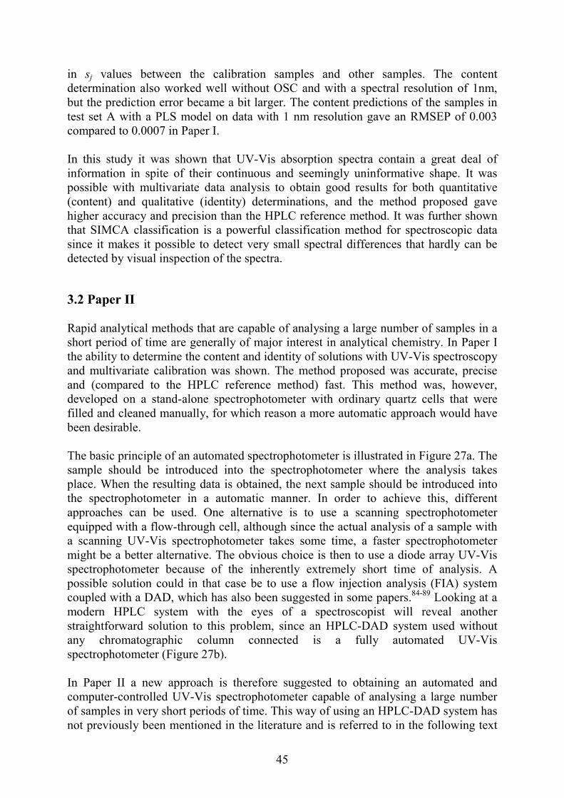
45

in sj values between the calibration samples and other samples. The content determination also worked well without OSC and with a spectral resolution of 1nm, but the prediction error became a bit larger. The content predictions of the samples in test set A with a PLS model on data with 1 nm resolution gave an RMSEP of 0.003 compared to 0.0007 in Paper I. In this study it was shown that UV-Vis absorption spectra contain a great deal of information in spite of their continuous and seemingly uninformative shape. It was possible with multivariate data analysis to obtain good results for both quantitative (content) and qualitative (identity) determinations, and the method proposed gave higher accuracy and precision than the HPLC reference method. It was further shown that SIMCA classification is a powerful classification method for spectroscopic data since it makes it possible to detect very small spectral differences that hardly can be detected by visual inspection of the spectra. 3.2 Paper II Rapid analytical methods that are capable of analysing a large number of samples in a short period of time are generally of major interest in analytical chemistry. In Paper I the ability to determine the content and identity of solutions with UV-Vis spectroscopy and multivariate calibration was shown. The method proposed was accurate, precise and (compared to the HPLC reference method) fast. This method was, however, developed on a stand-alone spectrophotometer with ordinary quartz cells that were filled and cleaned manually, for which reason a more automatic approach would have been desirable. The basic principle of an automated spectrophotometer is illustrated in Figure 27a. The sample should be introduced into the spectrophotometer where the analysis takes place. When the resulting data is obtained, the next sample should be introduced into the spectrophotometer in a automatic manner. In order to achieve this, different approaches can be used. One alternative is to use a scanning spectrophotometer equipped with a flow-through cell, although since the actual analysis of a sample with a scanning UV-Vis spectrophotometer takes some time, a faster spectrophotometer might be a better alternative. The obvious choice is then to use a diode array UV-Vis spectrophotometer because of the inherently extremely short time of analysis. A possible solution could in that case be to use a flow injection analysis (FIA) system coupled with a DAD, which has also been suggested in some papers.84-89 Looking at a modern HPLC system with the eyes of a spectroscopist will reveal another straightforward solution to this problem, since an HPLC-DAD system used without any chromatographic column connected is a fully automated UV-Vis spectrophotometer (Figure 27b). In Paper II a new approach is therefore suggested to obtaining an automated and computer-controlled UV-Vis spectrophotometer capable of analysing a large number of samples in very short periods of time. This way of using an HPLC-DAD system has not previously been mentioned in the literature and is referred to in the following text

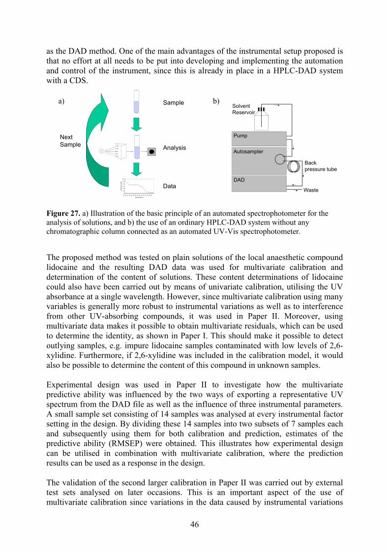
46

as the DAD method. One of the main advantages of the instrumental setup proposed is that no effort at all needs to be put into developing and implementing the automation and control of the instrument, since this is already in place in a HPLC-DAD system with a CDS. Figure 27. a) Illustration of the basic principle of an automated spectrophotometer for the analysis of solutions, and b) the use of an ordinary HPLC-DAD system without any chromatographic column connected as an automated UV-Vis spectrophotometer. The proposed method was tested on plain solutions of the local anaesthetic compound lidocaine and the resulting DAD data was used for multivariate calibration and determination of the content of solutions. These content determinations of lidocaine could also have been carried out by means of univariate calibration, utilising the UV absorbance at a single wavelength. However, since multivariate calibration using many variables is generally more robust to instrumental variations as well as to interference from other UV-absorbing compounds, it was used in Paper II. Moreover, using multivariate data makes it possible to obtain multivariate residuals, which can be used to determine the identity, as shown in Paper I. This should make it possible to detect outlying samples, e.g. impure lidocaine samples contaminated with low levels of 2,6-xylidine. Furthermore, if 2,6-xylidine was included in the calibration model, it would also be possible to determine the content of this compound in unknown samples. Experimental design was used in Paper II to investigate how the multivariate predictive ability was influenced by the two ways of exporting a representative UV spectrum from the DAD file as well as the influence of three instrumental parameters. A small sample set consisting of 14 samples was analysed at every instrumental factor setting in the design. By dividing these 14 samples into two subsets of 7 samples each and subsequently using them for both calibration and prediction, estimates of the predictive ability (RMSEP) were obtained. This illustrates how experimental design can be utilised in combination with multivariate calibration, where the prediction results can be used as a response in the design. The validation of the second larger calibration in Paper II was carried out by external test sets analysed on later occasions. This is an important aspect of the use of multivariate calibration since variations in the data caused by instrumental variations

DAD

Autosampler

Pump

Waste

Solvent Reservoir

Back pressure tube

b) Sample

Data

Analysis

Next Sample

0

20

40

60

80

100

120

245

248

251

254

257

260

263

266

269

272

275

278

281

284

287

Wavelength (nm)

Abs

orba

nce

(mA

U)

a)

47

or outer factors are more likely to arise over time. A general aim in multivariate calibration is also to be able to use the calibration over time without the need for recalibration. The prediction results obtained showed that the calibration model could be used over periods of time, obtaining precision, accuracy and repeatability in the same range as the reference method used in Paper II, HPLC. As discussed in Paper I, the time taken to scan a UV spectrum of a sample is less than the time taken to perform chromatography for separation and identification with external standards. The time to analyse a sample with an HPLC-DAD system without any chromatographic column connected is obviously even shorter, and the run time per sample in Paper II was 30s. In the methods used in Papers I and II the time of analysis per sample was for HPLC 5 min, scanning UV-Vis spectroscopy ∼1 min and diode array spectroscopy ∼0.5 min. The run time with the DAD method could probably be decreased even more if necessary by employing a higher flow rate, a shorter or wider back-pressure tube or by placing the back pressure tube after the detector. However, as mentioned in Paper II, a completely automatic data transfer procedure of the UV spectra to the calibration model would save more time, as discussed further in the next section. Comparing the results obtained with scanning UV-Vis spectroscopy in Paper I with the results of non-column chromatographic diode array UV spectroscopy in Paper II, it can be seen that the accuracy, precision and repeatability are slightly better with scanning UV-Vis spectroscopy. The high speed and automation obtained using the DAD technique, however, to a very large extent offset this in terms of higher analytical capacity, easier implementation etc. Furthermore, as previously mentioned, the identity determination in Paper I could also be performed with a spectral resolution of 1 nm, which is the same spectral resolution as with the DAD method. It should thus be possible with the SIMCA classification to distinguish the very similar UV spectra of, for instance, lidocaine and bupivacaine with the DAD method as well. Sources of error in the DAD method proposed are somewhat similar with some of the error sources in ordinary HPLC, such the accuracy and precision of the injections, the signal-to-noise ratio of the detector etc. The error sources related to the chromatography are, however, absent or less pronounced with the DAD method. One example is the pump flow, which is less crucial in the DAD method since the aim of the pump is simply to introduce the sample into the spectrophotometer (DAD). Furthermore, since no chromatography is used, no attention needs to be expended on factors influencing separation such as the composition of mobile phases, types of columns etc. In summary the main advantages of the DAD-method proposed are very rapid analysis, utilisation of the automation in the HPLC system and the lack of organic solvents needed. In Paper II the term high capacity analysis (HCA) was introduced, comprising spectroscopic analyses, chemometric data evaluation and a high level of automation. HCA methods could be very attractive for routine determinations in industrial quality control or for screening purposes, i.e. whenever the number of samples is large, an HCA method could be good choice of analytical method.

48

3.3 Paper III As previously described, calibration transfer is a serious problem when using multivariate spectroscopic calibration. Variations in the instrumentation in both the short and the long term can severely affect the prediction results. In applications using vibrational spectroscopy in solid samples a lot of work has been done and a large number of methods have been developed.44-48 In the multivariate applications involving solutions, however, the methods are much fewer49, although many of the methods developed for solids also work with liquids. Performing multivariate calibration on liquid samples, however, is generally easier to do since the construction of the calibration samples using solutions is simply a matter of dilution. In the analysis of solid samples the manufacturing of calibration samples of known content is more complicated. In Paper III a new approach is suggested in order to diagnose and correct errors in the predictions when the same multivariate calibration model is used over time. By analysing together with the unknown samples a control sample, i.e. a sample of known content and identity, and also by examining multivariate residuals of all the samples, reliable predictions over time using the same calibration model can be made. The use of control samples together with multivariate calibration has not previously been reported in the literature, although the use of instrument standardisation where a new set of samples is analysed and the results obtained are used for standardisation47-49 can be seen as a more complicated use of control samples. In Paper III the DAD method previously described in Paper II was used for multivariate determination of lidocaine samples and for testing the concept of control samples. If ordinary PLS is to be used on second order DAD data some reduction of the DAD file of each sample into a one-dimensional array must take place. (In Paper III it is misleadingly stated that it is essential to transform the data of each sample into a two-dimensional matrix. The dimensionality of DAD data is also somewhat unclearly described in Paper III. However, as explained in section 2.3.1, DAD data becomes three-way data when the absorbance is measured as a function of wavelength, time and samples.) In order to obtain one-way data, a representative UV spectrum must be exported from the DAD file and, as shown in Papers II and III, three possible ways of doing this are to export the maximum intensity spectrum (denoted SMIT in Papers II and III), the average spectrum over the sample peak or the average UV spectrum over the whole DAD file. As the results in Papers II and III show, these three methods give roughly equal results and the choice of which method to use is more a question of what is most convenient regarding automation and implementation. The methods using the average spectrum are, however, perhaps more easily implemented since the SMIT is not totally stable, i.e. some small retention time shifts are likely to arise. In Paper III a test set containing 15 lidocaine samples and one control sample was analysed with the DAD method on three separate occasions in order to investigate whether the use of a control sample could estimate and correct for the prediction error. From the results obtained it could be concluded that the control sample could indeed

49

diagnose the prediction error of the 15 samples and the prediction error of the control sample could also be used to correct the predictions. In Paper III the confidence interval for content determinations of the control sample was proposed as a limit to determine whether or not to correct the predictions of the unknown samples. It is possible that this limit also could be determined in other ways, although but the aim in Paper III was mainly to illustrate how the concept of using control samples could work in practise and the use of a confidence interval was in that case a good choice. It should be emphasised that investigation of the multivariate residuals of the unknown samples should be used together with the control sample since the residuals of the unknown samples gives valuable information on how these fit into the calibration model, as shown in Paper I. The idea of correcting the predictions may seem somewhat bold, especially in a highly regulated environment such as the pharmaceutical industry. Nevertheless, with the use of control samples and multivariate residuals, this might very well be a fully functional approach. It should be noted that the mobile phase used in Papers II and III, Milli-Q water, is not really an optimal solvent for use with the method proposed since it can be regarded as an unbuffered chemical. A more suitable solvent would be a phosphate buffer or suchlike that has been chosen with respect to the chemical properties of the compound analysed. It is also possible that for other types of samples, small amounts of a polar organic solvent such as acetonitrile might be needed in the mobile phase in order to wash out the previous sample properly from the detector cell. In Papers II and III plain lidocaine solutions were used, but there should be no obstacle to employing this type of method also for more complex samples (containing, for instance, excipients, degradation products and impurities) as long as this is taken in account in the calibration model. In Figure 4 in Paper III the joint practical procedure of the methods proposed in Papers I, II and III is summarised. This figure outlines how diode array UV-Vis spectroscopy, multivariate calibration, residuals and control samples can be used together in an HCA method. The same PLS calibration model is used for both determination of content and identity and the control samples are used as an external test of the reliability of the predictions obtained. In Papers II and III Excel macros were used to export the representative UV spectrum of each sample. This approach was fast but required the use of additional software and it was not completely automated. However, if the procedure proposed in Papers II and III could be supplemented with a fully automatic export of the representative UV spectrum of each sample as well as the content and identity predictions of it, i.e. to close the gap between the chemometric and the chromatographic software as illustrated in Figure 28, this would truly be an implementation of HCA.

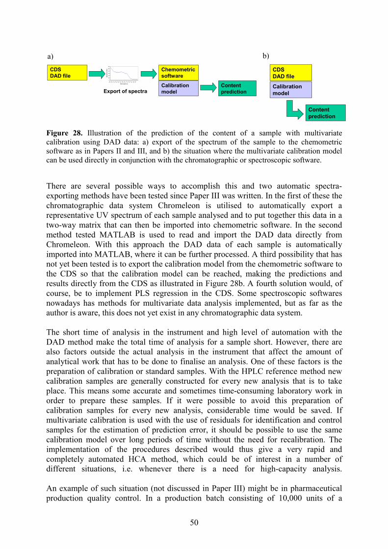
CDS

CDS Chemometric

60

80

100

120

banc

e (m

AU)

a)

50

Figure 28. Illustration of the prediction of the content of a calibration using DAD data: a) export of the spectrum of the sasoftware as in Papers II and III, and b) the situation where the mulcan be used directly in conjunction with the chromatographic or spe There are several possible ways to accomplish this and exporting methods have been tested since Paper III was writtenchromatographic data system Chromeleon is utilised to representative UV spectrum of each sample analysed and to ptwo-way matrix that can then be imported into chemometric method tested MATLAB is used to read and import the DChromeleon. With this approach the DAD data of each simported into MATLAB, where it can be further processed. A not yet been tested is to export the calibration model from the cthe CDS so that the calibration model can be reached, makresults directly from the CDS as illustrated in Figure 28b. A fcourse, be to implement PLS regression in the CDS. Some nowadays has methods for multivariate data analysis implemauthor is aware, this does not yet exist in any chromatographic The short time of analysis in the instrument and high level DAD method make the total time of analysis for a sample shalso factors outside the actual analysis in the instrument thanalytical work that has to be done to finalise an analysis. Onpreparation of calibration or standard samples. With the HPLCcalibration samples are generally constructed for every new place. This means some accurate and sometimes time-consumorder to prepare these samples. If it were possible to avcalibration samples for every new analysis, considerable timultivariate calibration is used with the use of residuals for idsamples for the estimation of prediction error, it should be pcalibration model over long periods of time without the neeimplementation of the procedures described would thus gcompletely automated HCA method, which could be of indifferent situations, i.e. whenever there is a need for An example of such situation (not discussed in Paper III) migproduction quality control. In a production batch consistin

DAD file

Calibration model

Content prediction

software0

20

40

24524

825

125

425

726

026

3266

269

272275

278281

284287

Wavelength (nm)

Abso

r

Export of spectra

b)

sample with multivariate mple to the chemometric tivariate calibration model ctroscopic software.

two automatic spectra-. In the first of these the automatically export a ut together this data in a software. In the second AD data directly from ample is automatically third possibility that has hemometric software to ing the predictions and ourth solution would, of spectroscopic softwares ented, but as far as the

data system.

of automation with the ort. However, there are

at affect the amount of e of these factors is the reference method new analysis that is to take ing laboratory work in

oid this preparation of me would be saved. If entification and control ossible to use the same d for recalibration. The ive a very rapid and terest in a number of high-capacity analysis.

ht be in pharmaceutical g of 10,000 units of a

DAD file

Calibration model

Content prediction

51

pharmaceutical solution, a number of samples (say 100) are taken out for after-control to ensure that their content and identity are within the given specification limits of the product. The only sample pre-treatment that might be necessary would be dilution of the samples before the analysis. The analysis is then rapidly performed with a HCA method where a few control samples are also analysed. A previously developed calibration model can be used since control samples and multivariate residuals ensure reliable predictions. Nowadays, however, there is a trend in the pharmaceutical industry towards the parametric release of pharmaceutical products i.e. performing the analyses directly in the production line using process analytical technology (PAT) and thereby eliminating the need for analysis of the final products. It is, however, the author’s firm belief that some levels of after-control will always remain even if parametric release is implemented in practise and so the need for HCA methods in the pharmaceutical industry will probably continue to exist in the future. It is also possible to implement HCA methods as PAT methods for the analysis of solutions directly on the production line. A further aspect of HCA methods is that this analytical approach fits very well into new effective and automated laboratories where large number of routine analyses are carried out. In Figure 29 a future vision of how an HCA method could be an important feature of the implementation of the ‘automated electronic laboratory’ is illustrated. Figure 29. An illustration of how HCA could be implemented as one important element of the ‘automated electronic laboratory’.

Analysis by HCA method

Spectra Database

Calibration model

Prediction Results

Electronic Laboratory Protocol

LIMS

Sample

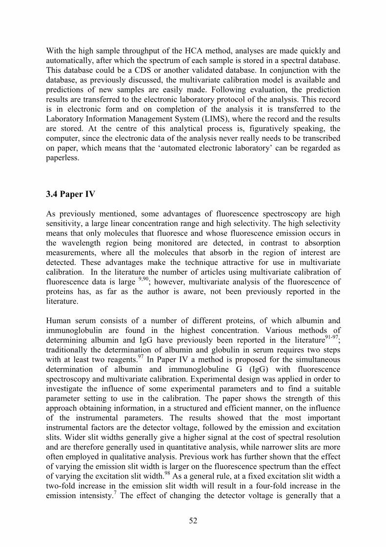
52

With the high sample throughput of the HCA method, analyses are made quickly and automatically, after which the spectrum of each sample is stored in a spectral database. This database could be a CDS or another validated database. In conjunction with the database, as previously discussed, the multivariate calibration model is available and predictions of new samples are easily made. Following evaluation, the prediction results are transferred to the electronic laboratory protocol of the analysis. This record is in electronic form and on completion of the analysis it is transferred to the Laboratory Information Management System (LIMS), where the record and the results are stored. At the centre of this analytical process is, figuratively speaking, the computer, since the electronic data of the analysis never really needs to be transcribed on paper, which means that the ‘automated electronic laboratory’ can be regarded as paperless. 3.4 Paper IV As previously mentioned, some advantages of fluorescence spectroscopy are high sensitivity, a large linear concentration range and high selectivity. The high selectivity means that only molecules that fluoresce and whose fluorescence emission occurs in the wavelength region being monitored are detected, in contrast to absorption measurements, where all the molecules that absorb in the region of interest are detected. These advantages make the technique attractive for use in multivariate calibration. In the literature the number of articles using multivariate calibration of fluorescence data is large 9,90; however, multivariate analysis of the fluorescence of proteins has, as far as the author is aware, not been previously reported in the literature. Human serum consists of a number of different proteins, of which albumin and immunoglobulin are found in the highest concentration. Various methods of determining albumin and IgG have previously been reported in the literature91-97; traditionally the determination of albumin and globulin in serum requires two steps with at least two reagents.97 In Paper IV a method is proposed for the simultaneous determination of albumin and immunoglobuline G (IgG) with fluorescence spectroscopy and multivariate calibration. Experimental design was applied in order to investigate the influence of some experimental parameters and to find a suitable parameter setting to use in the calibration. The paper shows the strength of this approach obtaining information, in a structured and efficient manner, on the influence of the instrumental parameters. The results showed that the most important instrumental factors are the detector voltage, followed by the emission and excitation slits. Wider slit widths generally give a higher signal at the cost of spectral resolution and are therefore generally used in quantitative analysis, while narrower slits are more often employed in qualitative analysis. Previous work has further shown that the effect of varying the emission slit width is larger on the fluorescence spectrum than the effect of varying the excitation slit width.98 As a general rule, at a fixed excitation slit width a two-fold increase in the emission slit width will result in a four-fold increase in the emission intensisty.7 The effect of changing the detector voltage is generally that a

53

higher detector voltage will increase the signal at the cost of higher electronic noise. A low setting is generally recommended for high emitting samples, while a high setting is recommended for low-emitting samples. The result of the quantitative determination of albumin and IgG showed that the determinations could be carried out with reasonable accuracy (albumin predictions within <±2 µg ml-1 and IgG1 within <±1 µg ml-1). A possible source of error in the proposed method in Paper IV is shifts in temperature, since fluorescence intensity generally increases with decreasing temperature. This can be overcome by thermoregulation of the cell compartment. Shifts in pH can also affect the fluorescence, since they can alter the ratio of charged and uncharged species in the solution. The use of the PBS buffer in Paper IV probably reduced this effect, since no influence on the fluorescence spectra caused by changes in pH were seen. In Paper IV the specified path length of the quartz cells used is incorrect. These had a path length of 10 mm and not nm as stated. In the two experimental design studies and in the screening calibration albumin was dissolved in Milli-Q water, while in the final larger calibration it was dissolved in PBS. The choice of PBS as solvent in the final calibration was due to the fact that it is a better solvent for proteins than Milli-Q. The purified water is also very pH-sensitive since it is un-buffered. The conclusions drawn from the experimental design study hold true, however, also for the albumin solutions in PBS, since neither PBS or Milli-Q water show any fluorescence and hence the fluorescence spectra of the two solvents are very similar and the solvents are considered to be equivalent. The fluorescence contribution from PBS is thus negligible and the optimum instrumental parameter setting found should also be valid also for solutions in PBS. With regard to the fluorescence of proteins, it is difficult to determine in advance their actual fluorescence from the number of tryptophan, tyrosine and phenylalanine residues since there are intricate relationships between the number of these amino acids, the overlap of emissions as well as outer factors like pH, the folding of the protein etc. As mentioned in Paper IV, the presence of Rayleigh and Raman scatter in the spectra does not seem to affect the predictive ability in any way. As shown in Figure 9 on page 17, the more intense Rayleigh scatter does not really exist in the wavelength regions used in Paper IV. The low-intensity Raman scatter, in contrast, can be found in the wavelengths used, although it did not affect the predictions made with the multivariate calibration. This shows the strength of multivariate data analysis using the whole spectrum instead of univariate data since the latter approach would most certainly be severely affected by this scatter. However, if multivariate data analysis is employed and mean centring is used as pre-processing, as in Paper IV, the Raman effect will disappear since the Raman intensity is constant in all samples. Without mean centring the PLS model would probably need an additional component in order to handle the Raman scatter, although this scatter would, most likely not affect the predictive ability of the model. This has also been described in a previous work.90

54

An attempt was also made to try to determine albumin and IgG in real serum samples collected from an albumin affinity column as well as purified serum samples collected from an experiment with coupled affinity columns for both albumin and IgG. The results obtained showed reasonable content predictions for both albumin and IgG in non-bound and bound fractions, although in a few fractions of the serum samples large residuals and high content predictions indicated differences from the calibration model. This is probably due to interfering fluorescence from other serum proteins, and the method needs to be developed further to allow albumin and IgG to be determined directly in serum samples, one possible way of doing this being to extend the calibration with other serum proteins. The method proposed did, however, show that the capacity of the albumin-binding column is lower than stated by the manufacturer, and the method could therefore be used to test the binding affinity of albumin chromatographic columns. Some calculations were also made in order to be able to determine the identity of albumin and IgG with the fluorescence spectra and SIMCA classification. The results obtained showed that it was possible to correctly determine the identity of both albumin and IgG. It remains for the future to see whether this identification can also be made for natural serum samples. Fluorescence spectroscopy might very well also be used in methods for HCA by the use of a fast fluorescence detector and diode-array detectors have also been proposed for spectrofluorometry.99 Furthermore, the use of fibre optic probes in fluorescence spectroscopy could be an interesting alternative for analysis of solutions. 3.5 Paper V As previously described in section 2.2, in liquid chromatography there is generally an ambition to obtain baseline-separated peaks. This ambition is mainly an effect of the traditional use of univariate detection and calibration since detection at a single wavelength needs completely separated peaks in order to selectively determine each compound. However, with the use of multivariate data and analysis, the need for baseline-separated peaks decreases, as is shown in Papers V and VI. The examples of different chemometric methods used to resolve partly separated peaks are numerous in the literature51-62 and many of these use PCA in some way or another. In EFA multiple PCA calculations are made on increasing portions of the eluting UV-Vis spectra in the DAD data matrix.51,52 This is done both in the forward analysis (starting with the first eluted spectra) and in the backward analysis (starting at the end of the chromatogram). Hence performing EFA on a sample used in Paper V consisting of 1500*46 data points involves something like 3000 PCA decompositions. It is thus no understatement to say that performing EFA is rather demanding in computational terms (compared to PCA). Generally, chemometric methods used for multivariate curve resolution aim to obtain the pure chromatographic, spectral and concentration profiles of all compounds in the sample analysed. A somewhat less complicated, but nevertheless important, question is whether or not a chromatographic peak is pure, i.e. arises from a single compound. Modern chromatographic data systems generally have some functions for the analysis of peak purity in their software. In Paper V the two methods (PPI and PPM) available

55

in the CDS used, Chromeleon, were employed as reference methods for peak purity determination. The peak purity index (PPI) is defined as the central wavelength of the spectrum where the areas of the left and right part of the spectrum is the same, and for a pure peak, the PPI would be the same for all spectra recorded over it.100 The peak purity match factor (PPM) describes the similarity of two spectral curves and can be determined by comparison of the spectra recorded over a peak.100 In Paper V a rapid and simple method for the determination of chromatographic peak purity is proposed. It is shown how a single PCA decomposition of the DAD data of a peak can be used to determine whether or not a peak is pure. The procedure proposed is called the PCA method. By performing a PCA decomposition with two PCs on the DAD data of a chromatographic peak and investigate the relative observation residuals of the first PC together with the scores and loadings of the second PC, information on the purity of the peak is given. Compared to EFA, this is a very simple calculation and the calculation time showed in Paper V for the PCA method was < 3 s, while the EFA took >20 min on a standard personal computer. The method was tested on binary mixtures of lidocaine and prilocaine at two levels of separation and the aim was to determine the peak purity of the major lidocaine peak in the presence of much lower levels of prilocaine. The results obtained showed that the method proposed is able to determine the major peak as impure in the same range as the detection limit of baseline-separated samples, outperforming the reference methods in the CDS used by a factor of ten. The explanation for this higher sensitivity for detecting impure peaks might be that the PCA decomposition is done simultaneously on all spectra collected over the chromatographic peak, in contrast to the PPI and PPM methods. As mentioned, the PPI method utilises the central wavelength of the spectra recorded over the peak, which means reducing each spectrum recorded to one value. The PPM works by comparing the peak apex spectrum with one of the other peak spectra at a time. By making this ‘two-spectra comparison’ between the apex spectrum and all the other spectra of the recorded peak, an estimate of the PPM is given. Hence, the two reference methods used for peak purity determination, PPI and PPM, do not employ all recorded spectra simultaneously like the PCA method. In Figure 30 the PCA decomposition of the two-way DAD data of a sample consisting of partly separated lidocaine and prilocaine peaks (RS=0.7) is illustrated with one PC according to X=t1p1′′′′ + E1. This figure shows three-dimensional plots of the raw DAD data, X (Figure 30a), the first PC, i.e. t1p1′′′′ (Figure 30b), and the residual matrix when the first PC has been calculated, E1 (Figure 30c). The figure is based on DAD data of a sample containing a somewhat higher prilocaine concentration than the samples used in Paper V, since the higher prilocaine content makes it easier to see how the PCA decomposition works and what variance it captures. For reasons of clarity this PCA decomposition was also made here without mean centring. In Figure 30a the raw DAD data of the sample is shown and, as can be seen, the prilocaine and lidocaine UV spectra are clearly seen as two closely eluting peaks. The smaller prilocaine peak elutes at around 3 minutes and the lidocaine peak at about 3.4 minutes. Figure 30b illustrates the three-dimensional plot of the first PC (t1p1′′′′) and the figure shows the variation explained in the first PC, a shape fairly similar to Figure

56

30a. Some important differences are present, however, since p1 mainly has captured the shape of the UV spectrum of lidocaine, this shape is also seen in both peaks in Figure 30b (p1 resembles the average spectrum in the DAD file as described in paper V). Furthermore the prilocaine peak in Figure 30b is actually slightly smaller than in the raw DAD data (Figure 30a) at 245–260 nm, while the opposite is true for 260–280 nm. This is also a consequence of the fact that the first PC is spectrally more related to lidocaine due to its higher concentration (and more specific UV spectrum) in the sample and causes residues of prilocaine. These remainders in E1 are seen around 3 minutes in Figure 30c at about 245–260 nm (a single positive ‘peak’) and 260–280 nm (a negative twin ‘peak’). If one compares the shape of the UV spectrum of the lidocaine peak at 3.4 minutes in Figure 30a and the corresponding loading in Figure 30b, it can be seen that they are also slightly different. The lidocaine spectrum in Figure 30a is sharper around 265 nm, while the corresponding loadings in Figure 30b are flatter, and this is the cause of the shape in the residual matrix E1 at 3.4 minutes (Figure 30c). It can be seen here that a large remainder of the lidocaine peak is present around 260–275 nm (the positive twin ‘peak’). Figure 30. Three-dimensional illustrations of the matrices of PCA decomposition of the DAD data of two partly separated peaks (133 mM lidocaine and 22 mM prilocaine, 17 conc. %). The chromatographic resolution was RS=0.7 a) raw DAD data (X), b) first PC (t1p1′′′′) and c) the residual matrix after the first PC has been determined (E1).

Wavelength (nm) Time (min)

Abso

rban

ce (m

AU

)

Wavelength (nm) Time (min)

t 1p1’

Wavelength (nm) Time (min)

Res

idua

l

a) b)

c)

57

The three-dimensional plots of a pure lidocaine sample (not shown here) would not show the smooth shape of the lidocaine spectrum in t1p1′′′′ seen in Figure 30b since it then should be no influence of prilocaine. Further should there be no pattern in the plot of E1 of a pure lidocaine sample (the small remainder of lidocaine peak seen in t2 and si/s0 in Paper V should hardly bee seen in the three dimensional plot of E1). For a sample with low concentration of prilocaine (like sample 5 in Paper V), the three-dimensional plot of the raw data X and t1p1′′′′ would be very similar to the corresponding plots of a pure lidocaine peak. However, the same shape of the remainder of prilocaine as in Figure 30c (though much smaller) would be seen in the three-dimensional plot of E1, making it possible to with scores and loadings to detect that the peak was actually impure. The small residue of lidocaine seen in pure lidocaine samples in Paper V is probably related to the peak and spectrum shape and not to a small level of non-linearity in the detector or variations in the injection or chromatographic process, as mentioned in Paper V. In the case of a tailing peak, the ‘average spectrum’ captured in p1 might be slightly different from the spectrum at peak apex due to the asymmetrical peak shape, and this slight difference might contribute to the small remainder. Moreover, the shape of the UV spectra of the compound in the chromatographic peak analysed might also influence the residue. However, the explanation of the small remainder of lidocaine in t2 and p2 of a pure lidocaine peak has not yet been thoroughly investigated. As shown above it is thus possible from the three-dimensional illustrations of the matrices in the PCA decomposition in Figure 30 to explain the shapes for the scores, loadings and relative observation residuals found in Paper V. As described in Paper V, the largest residue of the two compounds in E1 determines the direction of the second PC and the signs of the scores and loadings. If the prilocaine contribution is larger than the lidocaine contribution in E1 (as in the case of sample 3 in Paper V), it will determine the direction of PC2. If, however, the remainder of lidocaine in E1 is larger than the prilocaine contribution (as in the case of sample 5), it will determine the direction of PC2 and the scores and loadings will become rotated compared with sample 3. The rotation of p2 could thus serve as an indication of the concentration at which prilocaine can no longer be detected. Further parameters affecting the performance of the PCA method proposed might be the degree of spectral similarity between analyte and interferent, the signal-to-noise ratio in the DAD, the data collection rate etc. The position of the interfering peak in relation to the main peak might also influence the results, although this has not yet been sufficiently tested. The best way to determine whether the shapes of si/s0, t2 and p2 are indeed due to the presence of a second compound in the sample is to compare them with the shapes of a pure sample, as shown in Paper V. This is, however, more important when the content of the impurity is very low (about < 0.5 conc. %, although dependent on the compound analysed), whereas for higher concentration of impurities, the presence of additional peaks should be obvious when examining the relative observation residuals, scores and loadings without the need for comparison with the corresponding shapes of a pure peak. This is clearly shown in Figures 3a and b in

58

Paper V, where the presence of the impurity at about 3.1 minutes is obvious. Even without comparison with the profiles of the pure lidocaine sample, these plots reveals the presence of the small prilocaine peak. Hence the PCA method might also be used without the need for a pure sample. The PCA method was also tested on the same samples analysed without any chromatographic separation (RS=0), although it was then only possible to determine samples to be impure when the total absorbance of the two compounds were higher than the absorbance of a pure lidocaine sample. It can therefore be concluded that the PCA method is dependent on a small level of separation. The EFA calculations showed that the information regarding the chromatographic peak purity was the same as obtained with the PCA method. The interpretation of the EFA plots when the concentration of the minor compound is much lower than that of the major one is, however, not trivial, as shown in Paper V. The aim of EFA is, however, different to that of the PCA method since it tries to determine the number of compounds, their retention time windows and ultimately also their true spectra and concentrations. The aim of the PCA method, on the other hand, is in a rapid and simple manner to decide whether or not a chromatographic peak is pure, i.e. originating from a single compound. If the PCA method indicates an impure peak, this should preferably be evaluated with a new chromatographic experiment with better separation. It should be noted (as mentioned in Paper V) that a plot of the summed squared residuals of the first PC (Σe2) would show the same shape as the plot of si/s0, i.e. the same information regarding peak purity. It is thus possible to use this plot of the squared observation residuals (or squared ‘spectral residuals’) instead of the one described in Paper V. The reason for using si/s0 in Paper V was that it is a measure used in SIMCA classification, and this was also the measure initially used in the PCA method. The ratio of si/s0 is used in the SIMCA classification for comparing a single observation (like a spectrum) with the objects in the calibrated class, which is a supervised classification. However, since the PCA method is unsupervised, i.e. no a priori calibration is carried out, there should really be no need to make use of this ratio. The PCA method is rather used to illustrate the variance not explained (residuals) as well as the variance explained (t1 and p1) by the first PC, and a plot of Σe2 could very well be used for this issue. The proposed method could probably be implemented as a rapid method for peak purity determination since the calculations needed are simple and rapid. By continuously performing PCA on the eluting peaks, impurities in low levels could be detected.

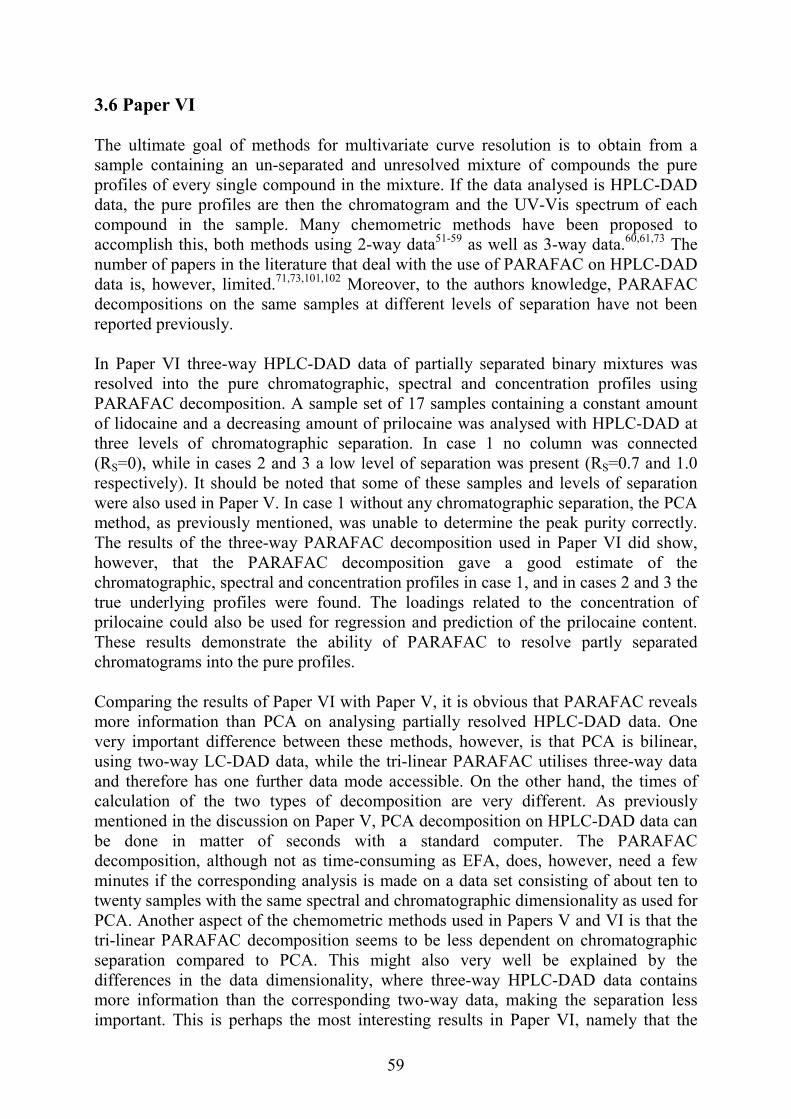
59

3.6 Paper VI The ultimate goal of methods for multivariate curve resolution is to obtain from a sample containing an un-separated and unresolved mixture of compounds the pure profiles of every single compound in the mixture. If the data analysed is HPLC-DAD data, the pure profiles are then the chromatogram and the UV-Vis spectrum of each compound in the sample. Many chemometric methods have been proposed to accomplish this, both methods using 2-way data51-59 as well as 3-way data.60,61,73 The number of papers in the literature that deal with the use of PARAFAC on HPLC-DAD data is, however, limited.71,73,101,102 Moreover, to the authors knowledge, PARAFAC decompositions on the same samples at different levels of separation have not been reported previously. In Paper VI three-way HPLC-DAD data of partially separated binary mixtures was resolved into the pure chromatographic, spectral and concentration profiles using PARAFAC decomposition. A sample set of 17 samples containing a constant amount of lidocaine and a decreasing amount of prilocaine was analysed with HPLC-DAD at three levels of chromatographic separation. In case 1 no column was connected (RS=0), while in cases 2 and 3 a low level of separation was present (RS=0.7 and 1.0 respectively). It should be noted that some of these samples and levels of separation were also used in Paper V. In case 1 without any chromatographic separation, the PCA method, as previously mentioned, was unable to determine the peak purity correctly. The results of the three-way PARAFAC decomposition used in Paper VI did show, however, that the PARAFAC decomposition gave a good estimate of the chromatographic, spectral and concentration profiles in case 1, and in cases 2 and 3 the true underlying profiles were found. The loadings related to the concentration of prilocaine could also be used for regression and prediction of the prilocaine content. These results demonstrate the ability of PARAFAC to resolve partly separated chromatograms into the pure profiles. Comparing the results of Paper VI with Paper V, it is obvious that PARAFAC reveals more information than PCA on analysing partially resolved HPLC-DAD data. One very important difference between these methods, however, is that PCA is bilinear, using two-way LC-DAD data, while the tri-linear PARAFAC utilises three-way data and therefore has one further data mode accessible. On the other hand, the times of calculation of the two types of decomposition are very different. As previously mentioned in the discussion on Paper V, PCA decomposition on HPLC-DAD data can be done in matter of seconds with a standard computer. The PARAFAC decomposition, although not as time-consuming as EFA, does, however, need a few minutes if the corresponding analysis is made on a data set consisting of about ten to twenty samples with the same spectral and chromatographic dimensionality as used for PCA. Another aspect of the chemometric methods used in Papers V and VI is that the tri-linear PARAFAC decomposition seems to be less dependent on chromatographic separation compared to PCA. This might also very well be explained by the differences in the data dimensionality, where three-way HPLC-DAD data contains more information than the corresponding two-way data, making the separation less important. This is perhaps the most interesting results in Paper VI, namely that the

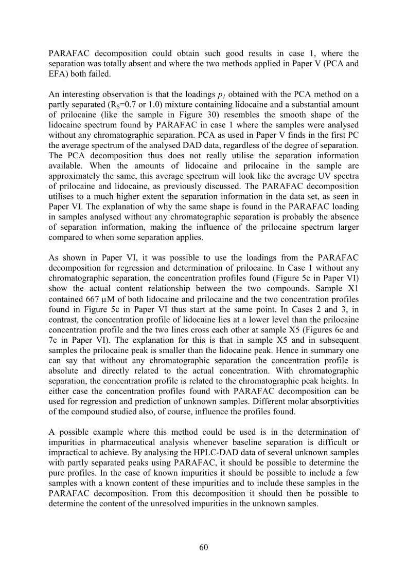
60

PARAFAC decomposition could obtain such good results in case 1, where the separation was totally absent and where the two methods applied in Paper V (PCA and EFA) both failed. An interesting observation is that the loadings p1 obtained with the PCA method on a partly separated (RS=0.7 or 1.0) mixture containing lidocaine and a substantial amount of prilocaine (like the sample in Figure 30) resembles the smooth shape of the lidocaine spectrum found by PARAFAC in case 1 where the samples were analysed without any chromatographic separation. PCA as used in Paper V finds in the first PC the average spectrum of the analysed DAD data, regardless of the degree of separation. The PCA decomposition thus does not really utilise the separation information available. When the amounts of lidocaine and prilocaine in the sample are approximately the same, this average spectrum will look like the average UV spectra of prilocaine and lidocaine, as previously discussed. The PARAFAC decomposition utilises to a much higher extent the separation information in the data set, as seen in Paper VI. The explanation of why the same shape is found in the PARAFAC loading in samples analysed without any chromatographic separation is probably the absence of separation information, making the influence of the prilocaine spectrum larger compared to when some separation applies. As shown in Paper VI, it was possible to use the loadings from the PARAFAC decomposition for regression and determination of prilocaine. In Case 1 without any chromatographic separation, the concentration profiles found (Figure 5c in Paper VI) show the actual content relationship between the two compounds. Sample X1 contained 667 µM of both lidocaine and prilocaine and the two concentration profiles found in Figure 5c in Paper VI thus start at the same point. In Cases 2 and 3, in contrast, the concentration profile of lidocaine lies at a lower level than the prilocaine concentration profile and the two lines cross each other at sample X5 (Figures 6c and 7c in Paper VI). The explanation for this is that in sample X5 and in subsequent samples the prilocaine peak is smaller than the lidocaine peak. Hence in summary one can say that without any chromatographic separation the concentration profile is absolute and directly related to the actual concentration. With chromatographic separation, the concentration profile is related to the chromatographic peak heights. In either case the concentration profiles found with PARAFAC decomposition can be used for regression and prediction of unknown samples. Different molar absorptivities of the compound studied also, of course, influence the profiles found. A possible example where this method could be used is in the determination of impurities in pharmaceutical analysis whenever baseline separation is difficult or impractical to achieve. By analysing the HPLC-DAD data of several unknown samples with partly separated peaks using PARAFAC, it should be possible to determine the pure profiles. In the case of known impurities it should be possible to include a few samples with a known content of these impurities and to include these samples in the PARAFAC decomposition. From this decomposition it should then be possible to determine the content of the unresolved impurities in the unknown samples.

61

It should be noted that shifts in the retention time and also in the chromatographic peak shape might result in departures from tri-linearity in the HPLC-DAD data, which in turn can influence the results of the PARAFAC decomposition. In Paper VI small retention time shifts were seen in only a few samples in case 1, and this was a minor problem that was corrected manually. When the number of retention time shifts is large, the PARAFAC2 algorithm72 can be applied. As mentioned in Paper VI, the PARAFAC decomposition was also tried only on samples X5–X17, where the prilocaine can be regarded as an impurity of low content compared to the lidocaine peak. The results obtained were the same as when the samples containing a higher amount of prilocaine were included, which shows that PARAFAC also works with low levels of impurities. The results obtained in Papers V and VI illustrates how the use of chemometric data analysis decreases the need for complete separation in chromatography. It is the author’s strong belief that chromatographic analyses in the future will be less focused on baseline separation with univariate detection in favour of multivariate detection on partly separated peaks evaluated by chemometric methods.

62

4. Conclusions This thesis has illustrated how spectroscopic techniques can be used in conjunction with chemometric tools in order to achieve rapid and simple analytical methods for the analysis of solutions. Paper I showed the strength of multivariate calibration and SIMCA classification on UV-Vis data for determination of the content and identity of pharmaceutical solutions. The paper illustrated how the same calibration model could be used for both quantitative and qualitative determinations. The results obtained were comparable or even slightly better than the reference method, HPLC. It was further shown that UV-Vis absorption spectra contain a great deal of information that can be utilised for classification and identity determination. In Paper II the method presented in Paper I was further developed with non-column chromatographic diode array UV spectroscopy using a conventional HPLC-DAD system without separation, giving a very fast analytical method with a high degree of automation. The main advantages of the method proposed are rapid analysis, automation and the absence of organic solvents. Paper III suggested a solution to the problem of using a calibration model over time. It was illustrated how a control sample of known identity and content could be used to diagnose and estimate the prediction error as well as to correct the predictions, thereby reducing the prediction error. If control samples are used together with investigation of multivariate residuals, this procedure could lead to an efficient analytical approach where the same calibration model could be used over time without recalibration. Paper IV illustrated the strength of using experimental design for finding a suitable instrumental setting as well as the use of multivariate calibration in fluorescence spectroscopy. Despite the overlapping fluorescence spectra of the two compounds in the study, the multivariate calibration with PLS regression was able to simultaneously determine their content. In Paper V it was shown how performing PCA on the DAD data of a chromatographic peak could be used to determine the peak purity. The compounds in the binary mixtures used had very similar spectra and the chromatograms showed substantial peak overlap. The method proposed could detect impure peaks where a minor impurity was of a much lower concentration (> 200 times) than a major one, thereby outperforming the reference methods in the CDS. The main advantage of this approach lies in its low ‘detection limit’ and its simplicity and ease of use. In Paper VI the ability of PARAFAC to extract the pure profiles of severely overlapping chromatographic peaks with very similar UV spectra was shown. Without any separation the PARAFAC decomposition gave a good estimate of the spectral and concentration profiles, and with a minimal level of separation the true underlying chromatographic, spectral and concentration profiles of the two compounds were

63

found. The study shows the strength of PARAFAC for resolving chromatographic peaks even with overlapping spectra and an absence of or very low levels of separation. The term high capacity analysis (HCA) was introduced as consisting of spectroscopic analysis, chemometric data evaluation and a high level of automation. Papers I–III outlined how UV-Vis absorption spectroscopy can be used for rapid and automated quantitative and qualitative determination of solutions with the help of chemometric techniques. Through investigation of multivariate residuals and use of control samples, the calibration model could also be used over time. Paper IV illustrated the strength of using fluorescence spectroscopy in multivariate calibration, and this spectroscopic technique might very well be used in HCA methods too. In Paper V a rapid and rather simple method for determining the purity of chromatographic peaks was suggested and in Paper VI the resolution of unresolved chromatographic profiles into pure spectra, chromatogram and concentrations was accomplished. The combined conclusion of Paper V and VI is that the need for baseline separation in chromatography is very low when chemometric data evaluation is used. In summary, these six papers show how chemometric tools such as experimental design, PCA, PLS, SIMCA and PARAFAC can be used to obtain efficient multivariate spectroscopic methods for the analysis of solutions.

64

5. Acknowledgements My supervisor, Professor Sven Jacobsson, for giving me the opportunity of

performing this work, enjoyable cooperation, discussions and support throughout. My assistant supervisor and manager, Dr Anders Hagman, for giving me the time and

opportunity to finish my PhD project as well as fruitful discussions. Peter Burén, for enjoyable collaboration and an excellent undergraduate thesis on UV-

Vis spectroscopy. Mattias Andersson, for fruitful cooperation and an exceptional undergraduate thesis on

Diode Array Detection UV-Vis spectroscopy. Agneta Sterner-Molin for enjoyable cooperation and an excellent undergraduate thesis

on fluorescence spectroscopy. Hans Pettersson for valuable discussions and tips regarding spectroscopy, HPLC,

Chromeleon etc. Dr Fredrik Andersson for valuable tips and tricks with MATLAB

Dr Mats Josefson for valuable discussions on SIMCA classification.

Professor Bo Karlberg for agreeable cooperation during my teaching periods at the

department of Analytical Chemistry. Magnus Åberg for enjoyable collaboration during the teaching periods at the

department. Barry Taylor for the invaluable work of checking the language of the manuscripts of

the papers as well as this thesis. Dr Anders Sparén for clarifying the mathematics of SIMCA classification.

All the agreeable and friendly individuals at the Department of Analytical Chemistry,

at SU, it has been a pleasure to get to know you! All of the staff at Analytical Development, AstraZeneca R&D Södertälje, for the nice,

friendly and open atmosphere that stimulates efforts like a PhD project. The crew of the “fishing machine” MS Trutta, Hasse, Peter and Johan, as well as the

members of “AEF”: Anders, Janne, Peter, Pär, Thomas and Danne, for reminding me that there other things in life than analytical research. I am convinced that new record catches of “havets silver” are about to come very soon... AstraZeneca plc for financial support during my PhD project.

My wife to be, dear Helén, for her never-ending unfailing patience, support and love,

and my daughter Amanda for being a ray of sunshine, inspirer and a wonderful little creature.

65

6. References

1. D. A. Skoog, J. J. Laery Principles of instrumental analysis Fourth edition, Saunders HBJ, 1992

2. T. Oven Fundamentals of modern UV-visible spectroscopy Hewlett Packard, 1996

3. L. E. Schoeff, R. H. Williams Principles of laboratory instruments Mosby, 1993

4. W. Kemp Organic Spectroscopy Macmillan press ltd, 1991

5. Guilbault George. G. Practical Fluorescence, 2nd edition Modern monographs in analytical chemistry, Marcel Dekker Inc, 1990

6. M. G. Gore Spectrophotometry and Spectrofluorimetry A Practical Approach, Oxford Press Oxford, 2000

7. Fluorescence, Cary Eclipse Software Manual

Varian, 2000

8. J. R. Lakowicz Principles of Fluorescence Spectroscopy Plenum Press, New York, 1990

9. R. A. Agbaria, P. B. Oldman, M. McCarrol, L. B. McGown, I. M. Warner Molecular Fluorescence, Phosphorescence, and Chemiluminescence Spectrometry Review, Analytical Chemistry 74 (2002) 3952–3962

10. G. E. P. Box , W. G. Hunter, J. S. Hunter Statistics for experimenters John Wiley& Sons, New York, 1978

11. N.R. Draper, H. Smith Applied regression analysis NewYork, John Wiley & Sons, 1981

12. D. L. Massart, B. G. M. Vandeginste, S. N. Deming, Y. Michotte, L. Kaufman Chemometrics: A textbook Elsevier, 1988

13. D. L. Massart, B. G. M. Vandeginste, L. M. C. Buydens, S. De Jong, P. J. Lewi, J. Smeyers-Verbeke Handbook of Chemometrics and Qualimetrics Elsevier, 1998

66

14. R. Brereton Chemometrics, Data Analysis for the laboratory and chemical plant Wiley , 2003

15. H. Martens and T. Naes, Multivariate Calibration Wiley, New York, 1989

16. R. Bro Håndbog i multivariabel kalibrering Jordbrugsforlaget, 1996

17. R. Nortvedt, F. Brakstad, O. M. Kvalheim, T. Lundstedt, eds. Anvendelse av kjemometri innen forskning og industri, Tidskriftsforlaget kjemi AS, 1996

18. L. Eriksson, E. Johansson, N. Kettaneh-Wold, S. Wold Multi- and Megavariate data analysis, principles and applications Umetrics, 2001

19. J.C. Miller, J. N. Miller Statistics for Analytical Chemistry Ellis Horwood Limited, 1993

20. A. K. Smilde, Y. Wang, B. Kowalski Theory of medium-rank second order calibration with restricted-Tucker models Journal of Chemometrics 8 (1994) 21–36

21. J. E. Jackson A users guide to principal components John Wiley & Sons, New York, 1991

22. S. Wold, K. Esbensen, P. Geladi Principal Component Analysis Chemometrics and Intelligent Laboratory Systems 2 (1987) 37–52

23. P. Geladi, B. Kowalski Partial least-squares regression: a tutorial Analytica Chimica Acta 185 (1986) 1–17

24. S. Wold, M. Sjöström, L. Eriksson

PLS-regression: a tool of chemometrics Chemometrics and Intelligent Laboratory Systems 58 (2001) 109–130

25. R. Bro PARFAC. Tutorial and applications Chemometrics and Intelligent Laboratory Systems 38 (1997) 149–171

26. R. Bro

Multiway calibration. Multilinear PLS Journal of Chemometrics 10 (1996) 47–61

67

27. L. R. Tucker Some mathematical notes on three-mode factor analysis Psychometrika 31 (1966) 279–311

28. A. de Juan, R. Tauler Comparison of three-way resolution methods for non-trilinear chemical data sets Journal of Chemometrics 15 (2001) 749–772

29. H. A. L. Kiers Towards a standardized notation and terminology in multiway analysis Journal of Chemometrics 14 (2000) 105–122

30. S. Wold Cross-validatory estimation of the number of components in factor and principal components models Technometrics 20 (1978) 397–405

31. L. Eriksson, E. Johansson, N. Kettaneh-Wold, C. Wikström, S. Wold Design of experiments, principles and applications Umetrics, 2000

32. S. N. Deming, S. L. Morgan, Experimental design: a chemometric approach Data handling in science and technology-vol 3, Elsevier, 1987

33. D. Morgan, Experimental design: a chemometric approach 2nd ed. Amsterdam, Elsevier 1989

34. R. A. McLean, V. L. Anderson Applied factorial and fractional designs Marcel Dekker Inc, 1984

35. R.J. Barnes, M.S. Dhanoa, S.J. Lister, Standard normal variate transformation and de-trending of near-infrared diffuse reflectance Spectra Applied. Spectroscopy 43 (1989) 772–777

36. S. Wold, H. Antti, F. Lindgren, J. Öhman Orthogonal Signal Correction of near-infrared spectra Chemometrics and Intelligent Laboratory Systems 44 (1998) 175–185

37. O. Svensson, T. Kourti, J. F. MacGregor An investigation of orthogonal signal correction algorithms and their characteristics Journal of Chemometrics 16 (2002) 176–188

38. L. Baibing, J. Morris, E. B. Matrin Orthogonal signal correction: algorithmic aspects and properties Journal of Chemometrics 16 (2002) 556–561

39. R. G. Brereton Introduction to multivariate calibration in analytical chemistry The Analyst 125 (2000) 2125–2154

68

40. M. Sjöström and S. Wold, Multivariate calibration problem in analytical chemistry solved by partial least squares models in latent variables Analytica Chimica Acta, 150 (1983) 61–70

41. R. Szostak, S. Mazurek Quantitative determination of acetylsalicylic acid and acetoaminophen in tablets by FT-Raman spectroscopy The Analyst 127 (2002) 144–148

42. M. Otto, W. Wegscheider Spectrophotometric multicomponent analysis applied to trace metals determination Analytical Chemistry 57 (1985) 63–69

43. ASTM standard, designation: Standard Practices for Infrared, Multivariate, Quantitative Determination, E 1655-94ε1

44. Feudale, N. A. Woody, H. Tan, A. J. Myles, S. D. Brown, J. Ferré Transfer of multivariate calibration models; a review Chemometrics and Intelligent Laboratory Systems 64 (2002) 181–192

45. S. Adhihetty, J. A. McGuire, B. Wangmaneerat, T. M. Niemczyk, D. M. Haaland Achieving transferable multivariate spectral calibration models: demonstration with infrared spectra of thin-film dielectrics on silicon Analytical Chemistry 63 (1991) 2329–2338

46. H. Swierenga, W. G. Haanstra, A.P. de Weijer, L. M. C. Buydens Comparison of two different approaches toward model transferability in NIR spectroscopy Applied Spectroscopy 52 (1998) 7–16

47. E. Bouveresse, C. Hartmann, D. L. Massart, I. R. Last, K. A. Prebble Standardization of near-infrared spectrometric instruments Analytical Chemistry 68 (1996) 982–990

48. Y. D. Wang, D. J. Veltkamp, B. R. Kowalski Multivariate instrument standardization Analytical Chemistry 63 (1991) 2750–2756

49. F. Sales, M. P. Callao, F. X. Rius Multivariate standardisation techniques using UV-Vis data Chemometrics and Intelligent Laboratory Systems 38 (1997) 63–73

50. T. Hirschfeld

The hy-phen-ated methods Analytical Chemistry 52 (1980) 297A–305A

51. M. Maeder, A.D. Zuberbuehler The resolution of overlapping peaks by evolving factor analysis Analytica Chimica Acta 181 (1986) 287–291

52. M. Maeder Evolving factor analysis for the resolution of overlapping chromatographic peaks Analytical Chemistry 59 (1987) 527–530

69

53. B. G. M. Vandeginste, W. Derks, G. Kateman Multicomponent self modelling curve resolution in high performance liquid chromatography by iterative target transformation analysis Analytica Chimica Acta 173 (1985) 253-264

54. H. R. Keller, D. L. Massart Peak purity control in liquid chromatography with photodiode-array detection by fixed size moving window evolving factor analysis Analytica Chimica Acta 246 (1991) 379–390

55. E. R. Malinowski Window factor analysis: theoretical derivation and application to flow injection analysis data Journal of Chemometrics 6 (1992) 29–40

56. O. M. Kvalheim, Y. Liang Heuristic evolving latent projections: resolving two-way multicomponent data. 1. Selelctivity, latent-projective graph, datascope, local rank, and unique resolution Analytical Chemistry 64 (1992) 936–946

57. Y. Liang, O. M. Kvalheim, H. R, Keller, D.L. Massart, P. Kiechle, F. Erni Heuristic evolving latent proejctions: Resolving two-way multicomponent data. 2. Detection and resolution of minor constituents Analytical Chemistry 64 (1992) 946–953

58. J. Toft, O. M. Kvalheim Eigenstructure tracking analysis for revealing noise pattern and local rank in instrumental profiles: application to transmittance and absorbance IR spectroscopy Chemometrics and Intelligent Laboratory Systems 19 (1993) 65–73

59. R. Tauler Multivariate curve resolution applied to second order data Chemometrics and Intelligent Laboratory Systems30 (1995) 133–146

60. E. Sánchez, B. R. Kowalski Generalized rank annihilation factor analysis Analytical Chemistry 58 (1986) 496–499

61. E. Sánchez, B. R. Kowalski Tensorial resolution: a direct trilinear decomposition Journal of Chemometrics 4 (1990) 29–45

62. J. C. Hamilton, P. Gemperline Mixture anslysis using factor analysis. II: self-modeling curve resolution Journal of Chemometrics 4 (1990) 1–13

63. S. Wold Pattern recognition by means of disjoint principal components models Pattern recognition 8 (1976) 127–139

64. W.J. Dunn, S. Wold, SIMCA Pattern Recognition and Classification Methods and Principles in Medicinal Chemistry 2 (1985) 179–193

70

65. R.De Maesschalck, A. Candolfi, D.L. Massart, S. Heuerding Decision criteria for soft independent modelling of class analogy applied to near infrared data Chemometrics and Intelligent Laboratory Systems 47 (1999) 65–77

66. B. Mertens, M. Thompson and T. Fearn Pincipal component outlier detection and SIMCA: a synthesis The Analyst 119 (1994) 2777–2784

67. R.B. Cattell Parallel proportional profiles and other principles for determining the choice of factors by rotation Psychometrika 9 (1944) 267

68. J. D. Carroll, J. Chang Analysis of individual differences in multidimensional scaling via an N-way generalisation of Eckart-Young decomposition Psychometrika 35 (1970) 283–319

69. J. B. Kruskal More factors than subjects, test and treatments: An interdeterminancy theorem for canonical decomposition and individual differences scaling Psychometrika 41 (1976) 281–293

70. R.A. Harshman Foundations of the PARAFAC procedure: models and conditions for an explanatory multi-mode factor analysis University of California at Los Angeles, UCLA Working Papers in Phonetics, 16 (1970) 1

71. P. Hindmarch, K. Kavianpour, R. G. Brereton Evaluation of parallel factor analysis for the resolution of kinetic data by diode-array high-performance liquid chromatography The Analyst 122 (1997) 871–877

72. H. A. L. Kiers, J. M. T. Ten Berge, R. Bro PARAFAC2-PartI. A direct fitting algorithm for the PARAFAC2 model Journal of Chemometrics 13 (1999) 275–294

73. R. Bro, C. A. Andersson, H. A. L. Kiers PARAFAC2-PartII. Modeling chromatographic data with retention time shifts Journal of Chemometrics 13 (1999) 295–309

74. M. Karlsson, B. Karlberg, R. J. O. Olsson Determination of nitrate in municipal waste water by UV spectroscopy Analytica Chimica Acta 312 (1995) 107–113

75. E. Engström, B. Karlberg, Screening method for metals based on array spectrophotometry and multivariate analysis Journal of Chemometrics 10 (1996) 509–520

76. R.D. Bautista, A.I. Jiménez, F. Jiménez, J.J. Arias, Simultaneous determination of diazepam and pyridoxine in synthetic mixtures and pharmaceutical formulations using graphical and multivariate calibration-predictios methods Journal of Pharmaceutical and Biomedical Analysis 15 (1996) 183–192

71

77. Z. Bouhsain, S. Garrigues, M. de la Guardia PLS-UV spectrophotometric method for the simultaneous determination of paracetamol, acetylsalicylic acid and caffeine in pharmaceutical formulations Fresenius Journal of Analytical Chemistry 357 (1997) 973–976

78. C. Demir, R.G. Brereton,

Multivariate calibration on designed mixtures of four pharmaceuticals The Analyst, 123 (1998) 181–189

79. T. Kappes, G. López-Cueto, J. F. Rodriguez-Medina, C. Ubide, Improved selectivity in multicomponent determinations through interference modelling by applying partial least squares regression to kinetic profiles The Analyst 123 (1998) 2071–2077

80. P. Gratteri, G. Cruciani, Experimental design and multivariate calibration in the development, set-up and validation of a differential pulse polarographic and UV spectrophotometric method for the simultaneous plasmatic determination of the therapeutic metronidazole-pefloxacin combination The Analyst 124 (1999) 1683–1688

81. M. M. Sena, J.C.B. Fernandes, L.,Jr Rover, R.J. Poppi, L.T. Kubota, Application of two- and three-way chemometric methods in the study of acetylsalicylic acid and ascorbic acid mixtures using ultra-violet spectrophotometry Analytica Chimica Acta 409 (2000) 159–170

82. J. Dahlén, S. Karlsson, M. Bäckström, J. Hagberg, H. Pettersson Determination of nitrate and other water quality parameters in groundwater from UV/Vis spectra employing partial least squares regression Chemosphere 40 (2000) 71–77

83. I. D. Merás, A. Espinosa Mansilla, F. Salinas López, M. J. Rodríguez Gómez, Determination of triamterene and leucovorin in biological fluids by UV derivative-spectrophotometry and partial least-squares (PLS-1) calibration Journal of Pharmceutical and Biomedical. Analysis 27 (2002) 81–90

84. C. Ridder, L. Nørgaard Simultaneous determination of cobalt and nickel by flow injection analysis and partial least-squares regression with outlier detection Chemometrics and Intelligent Laboratory Systems 14 (1992) 297–303

85. L. Nørgaard, C. Ridder Spectrophotometric determination of mixtures of 2-hydroxybenzaldehyde, 3-hydroxybenzaldehyde, and 4-hydroxybenzaldehyde by flow-injection analysis and UV-Vis photodiode-array detection Talanta, 41 (1994) 59–66

86. E. Bechmann, L. Nørgaard, C. Ridder Generalized standard addition in flow-injection analysis with UV-Visible photodiode array detection Analytica Chimica Acta 304 (1995) 229–236

72

87. O. Hernández, F. Jiménes, A. I. Jiménes, J.J. Arias, J. Havel, Multicomponent flow injection based analysis with diode array detection and partial least squares multivariate calibration evaluation. Rapid determination of Ca(II) and Mg(II) in waters and dialysis liquids Analytica Chimica Acta 320 (1996) 177–183

88. M. Azubel, F. M. Fernández, M. B. Tudino, O. E. Troccoli Novel application and comparison of multivariate calibration for the simultaneous determination of Cu, Zn and Mn at trace levels using flow injection diode array spectrophotometry Analytica Chimica Acta 398 (1999) 93–102

89. F. M. Fernández, M. B. Tudino, O. E. Troccoli, Multicomponent kinetic determination of Cu, Zn, Co, Ni and Fe at trace levels by first and second order multivariate calibration Analytica Chimica Acta 433 (2001) 119–134

90. L. Nørgaard A multivariate chemometric approach to fluorescence spectroscopy Talanta 42 (1995) 1305–1324

91. B.F. Rocks, S.M. Wartel, R.A.Sherwood, C. Riley

Determination of albumin with bromocresol purple using controlled-dispersion flow analysis The Analyst 110 (1985) 669–671

92. J. Nakamura, S. Igarashi

Highly sensitive spectrophotometric and spectrofluorometric determinations of albumin with 5,10,15,20-tertrakis(4-sulfophenyl) porphine Analytical Letters 29 (1996) 981–989

93. Huang C.Z., Zhu J.X., Li K.A., Tong S.Y.

Determination of albumin and globulin at nanogram levels by a resonance light-scattering technique with alpha, beta, gamma, delta-tetrakis(4-sulphopehnyl)porphine Analytical Science 13 (1997) 263–268

94. N.T. Deftereos, N. Grekas, A.C.Calokerinos

Flow injection chemiluminometric determination of albumin Analytica Chimica Acta 403 (2000) 137–143

95. H.R. Liang, M.K.Scott, D.J.Murry, S.M.Sowinski

Determination of albumin and myoglobin in dialysate and ultrafiltrate samples by high-performance size-exclusion chromatography Journal of Chromatography B 754 (2001) 141–151

96. K. Murayama, K. Yamada, R. Tsenkova, Y. Wang, Y. Ozaki

Near-infrared spectra of serum albumin and χ-globulin and determination of their concentrations in phosphate buffer solutions by partial least squares regression Vibrational Spectroscopy 18 (1998) 33–40

97. D.-H. Li, H.-H. Yang, H. Zhen, Y. Fang, Z. Q.-Z. Zhu., J.-G. Xu

Fluorimetric determination of albumin and globulin in human serum using tetra-substituted sulphonated aluminium phtalocyanine Analytica Chimica Acta 401 (1999) 185–189

73

98. L. Nørgaard Spectral resolution and prediction of slit widths in fluorescence spectroscopy by two- and three-way methods Journal of Chemometrics 10 (1996) 615–630

99. R. B. Poe, S. C. Rutan

Effects of resolution, peak ratio and sampling frequency in diode-array fluorescence detection in liquid chromatography Analytica Chimica Acta 283 (1993) 845–853

100. User´s Guide to Chromeleon Version 6.11 Dionex Sunnyvale, CA 2000

101. J.L. Beltrán, J. Guiteras, R. Ferrer Parallel factor analysis of partially resolved chromatographic data Determination of polycyclic aromatic hydrocarbons in water samples Journal of Chromatography A 802 (1998) 263–275

102. H.L. Wu, M. Shibukawa, K. Oguma An alternating trilinear decomposition algorithm with application to calibration of HPLC-DAD for simultaneous determination of overlapped chlorinated aromatic hydrocarbons Journal of Chemometrics 12 (1998) 1–26