Embed Size (px)
Citation preview

Monetizing the Value of Social Investments the low income investment fund’s approach to impact assessment
december 2015www.liifund.org/calculator
table of contents
1 Introduction
2 Executive Summary
6 Affordable HousingIn the area of affordable housing, we monetize the value of subsidized
rental housing on discretionary income, and on human health—as a remedy
for food insecurity, as a “vaccine” for homeless populations, and as vehicle
to enable families to “buy health” by moving to a healthier location.
30 Early Care and EducationIn the area of early care and education, we monetize long-term individual
and societal benefits, including health improvements later in life.
35 EducationIn the area of charter school finance, we estimate societal benefits and
long-term income boosts for students who attend high-performing schools.
38 Community Health ClinicsIn our health clinic financing, we estimate the economic value of producing
better health outcomes, delivering more efficient forms of care, and
preventing costly downstream hospitalizations and emergency room visits.
All impact estimates for metrics detailed in this document are in nominal, unadjusted dollars. However, it can be helpful to discount these benefits to current dollars in order to make “apples to apples” comparisons between costs and benefits that occur at different points in time—especially if some impacts are far into the future. The online version of the Social Impact Calculator allows users to discount benefits according to their choice of social discount rate, as well as calculate their internal rate of social return based on their investment. In addition, the Excel download that is available on the website allows users to see when impact occurs.

1
introductionLIIF is committed to expressing the social value of the projects that we support. In most
cases, however, we are not in the position to collect longitudinal data to track outcomes,
let alone determine impact (i.e., answering the counterfactual question of what would have
happened but for the intervention that LIIF supported). Still, high quality social science
research exists that can help address many of the “but for” questions in the program areas
where LIIF invests.
Our approach relies on leveraging the best available academic research in a common-
sense manner. We estimate impact and monetized value based on output proxies that we
can collect in the normal course of our business. We periodically update our approach
to account for advances in research and our evolving understanding of the value of the
projects that we support. LIIF focuses on social impact indicators that are central to our
mission of poverty alleviation, and relate to our “impact pathways” or program areas:
affordable housing, early learning, education, health, and equitable transit oriented
development.
We fully recognize that our approach monetizing impact “by proxy” is imprecise and falls
short of rigorous evaluation. In addition, most of our monetary estimates do not account
for the time value of money. However, we think it is important to take a first step toward
measuring the social value of community investments. Our approach is simple, but it is
practical given our institutional setting and limitations. At the portfolio and sector level, we
believe it is directionally accurate.
This document describes our approach to estimating a range of impacts—for the families we
serve, and for society at large. We update our methodology on a periodic basis to account
for changes in practice, advances in research, and our evolving understanding of the value
of the projects that we support.
2
executive summaryIn order to evaluate LIIF’s effectiveness in achieving our mission of poverty alleviation, we developed the
Social Impact Calculator—a way to calculate the dollar social value of the projects we support. The metrics
we developed for the Social Impact Calculator monetize the impact of our investments, and relate to
LIIF’s program areas: affordable housing, early learning, education, health, and equitable transit oriented
development. LIIF is not in the position to collect longitudinal data on each project. Therefore, the calculator
uses an impact-by-proxy approach that leverages academic research to translate project data that we collect
in our normal course of business into dollar estimates of social impact. By sharing its full methodology, LIIF
seeks to be transparent in our approach and encourage others to discuss, use, and improve upon our work.
n Affordable Housing
Income Boosts from Affordable Housing. The high cost of housing is one of the most pressing challenges
facing low- and moderate-income households today. More than half of households earning less than
$30,000 per year spend over half their income on rent, forcing painful tradeoffs and leaving little for other
basic necessities such as food, medical care, and transportation.1 We estimate the boost in discretionary
income generated by LIIF-supported affordable housing projects as the difference between market and
affordable rents, assuming that this impact holds for the project’s affordability restriction period.
Buying a Healthy Location: How Affordable Housing in Low-Poverty Areas Generates Positive
Diabetes and Obesity Outcomes. We draw on evidence from the U.S. Department of Housing and
Urban Development’s Moving to Opportunity (MTO) experiment to estimate the health value of housing’s
location—in particular, the finding that moving from public housing in a high-poverty area to a relatively
low-poverty neighborhood generated large reductions in diabetes and extreme obesity among women.2
We use this evidence to model health improvements by increasing access to low-poverty, “healthy”
communities—specifically, those in areas that meet the same criteria for “opportunity” neighborhoods that
MTO used. We draw on evidence on annual medical costs associated with diabetes and extreme obesity to
estimate medical cost savings generated over a project’s affordability restriction term.
Lifetime Earnings Boost from Accessing Low-Poverty Neighborhoods. A study of long-term effects
on children from MTO families published in 2015 revealed that, by their mid-20s, MTO participants in the
experimental group who moved from high-poverty neighborhoods to low-poverty areas before age 13
experienced a range of positive social effects—including higher earnings—relative to the control group that
1 Joint Center for Housing Studies of Harvard University. 2013. “The State of the Nation’s Housing 2013.” JCHS tabulations of US Census Bureau, American Community Surveys.2 Ludwig et al, New England Journal of Medicine summary of MTO found that a 10 percent drop in poverty was associated with reductions of 6.2, 4.3, and 3.2 percentage points, respectively, for class II and class III obesity, and diabetes.
3
had not been detected at the final of the original MTO final impacts evaluation.3 We use this study’s finding
on long-term earnings increases to estimate the same kind of impact on children who gain access to LIIF-
supported affordable housing projects in low-poverty neighborhoods.
Affordable Housing as a Remedy for Food Insecurity. Children who do not have adequate nutrition
are less healthy, suffer developmental impairments, and have lower educational achievement.4 Recent
studies have uncovered a strong correlation between housing costs and food insecurity.5 To estimate the
impact of LIIF-supported affordable housing on food expenditures, we draw from Bureau of Labors Statistics
Consumer Expenditure Survey (CES) data, reported in the 2013 “State of the Nation’s Housing” by the Joint
Center for Housing Studies of Harvard University,6 showing that families in the bottom expenditure quartile
(a very conservative proxy for low-income) who live in housing that is affordable to them spend significantly
more on food when compared to their counterparts who are more burdened by housing costs.7 We model
this incremental increase in food expenditures over the term of each project’s affordability restrictions.
Housing as a Vaccine: Improved Health Outcomes and Medical Cost Savings from Permanent
Supportive Housing for the Homeless. Permanent supportive housing is well known as an effective
strategy for improving life outcomes for the chronically homeless—particularly those with chronic and
complex illnesses. This intervention also generates significant public cost savings, primarily from reduced
health services. We draw from a 2009 study8 by the Economic Roundtable to estimate medical cost savings
generated by LIIF-supported permanent supportive housing projects.9
3 Source: Chetty, Raj, Nathaniel Hendren, and Lawrence F. Katz. 2015. The Effects of Exposure to Better Neighborhoods on Children: New Evidence from the Moving to Opportunity Experiment. The Equality of Opportunity Project. May.4 Cook, John, and Karen Jeng. 2009. “Child Food Insecurity: The Economic Impact on our Nation. A report on research on the impact of food insecurity and hunger on child health, growth and development commissioned by Feeding America and the ConAgra Foods Foundation.”5 See, for example: Fletcher, et al. 2009. “Assessing the effect of changes in housing costs on food insecurity.” Journal of Children and Poverty: Vol. 15, No. 2, 79-93.6 Joint Center for Housing Studies of Harvard University. 2013. “The State of the Nation’s Housing 2013.” JCHS tabulations of US Census Bureau, American Community Surveys.7 Bureau of Labor Statistics, 2011. Consumer Expenditure Survey. Website: http://www.bls.gov/cex/ Also cited in: The State of the Nation’s Housing 2012. Joint Center for Housing Studies of Harvard University.8 Economic Roundtable. 2009. “Where We Sleep: Costs when Homeless and Housed in Los Angeles.” 9 We chose this study based quality of the data available to the authors, the comprehensiveness (across multiple risk factors such as mental health status, substance abuse problems, and HIV/AIDS) and size of the study population, and the fact that its savings figure falls somewhere in the middle of the ranges in medical cost savings quoted in other studies. As such, it seemed to be a reasonable but conservative estimate to apply to the LIIF portfolio of permanent supportive housing projects.
4
Healthier Commutes: Equitable Transit-Oriented Development as a Strategy to Increase Physical
Activity and Boost Health. Transit-oriented development (TOD) has been shown to generate positive
human health outcomes through multiple pathways—for example, by increasing physical activity, or by
improving access to health-promoting services and amenities. Further, equitable TOD—which incorporates
housing and services targeted to lower- and moderate-income households—can create and preserve access
to these health benefits for these populations, and thus can serve as a critical platform for addressing health
disparities and inequality. To estimate health improvements from our TOD investments, we draw from the only
available experimental evidence demonstrating that increasing access to transit generates measurable health
improvements—a 2010 longitudinal study of people living near the South Corridor Light Rail line in Charlotte,
North Carolina before and after it became operational, setting the stage for a “natural experiment.” To estimate
medical cost savings generated by LIIF-supported TOD projects, we pair this study’s findings on weight loss
associated with commuting by transit with evidence on ridership near transit, and medical costs associated
with losing weight. We assume an impact period equivalent to the project’s affordability restriction term.
n Early Care and Education
Societal Benefits from Early Care and Education. Several recent studies have used data from multiple
random assignment experiments to propose estimates for early care and education’s long-term societal
benefits, ranging from $7 to $20 in societal returns per dollar invested. We take a conservative approach and
assume $7 in returns per dollar invested—the figure that President Obama cited in his State of the Union
address in 2013—generated by a combination of increased family income, educational attainment, and
reduced societal costs such as incarceration and special education. We calculate impact over the term of
LIIF’s grant to the child care center—a conservative assumption, since the centers usually continue to serve
children from low- and moderate-income families for many years after our grant term ends.
Buying Adult Health with Early Care and Education. Early care and education helps children develop
the cognitive functions and skills necessary to lead successful, healthy lives. A path breaking study by Nobel
Laureate James Heckman, Frances Campbell, and colleagues provides compelling evidence, based on a
randomized control trial, that high quality early care can deliver substantial health benefits that persist into
adulthood—in particular, dramatic reductions in the prevalence of metabolic syndrome, which is associated
with greater risk of heart disease, stroke, and type 2 diabetes.10 We use these findings to estimate similar
impacts for children in LIIF-supported early care and education centers, making appropriate assumptions
about the level of impact that these centers realistically deliver. Leveraging evidence on medical costs
associated with metabolic syndrome, we then calculate cost savings associated with reduced prevalence of
metabolic syndrome over a conservative time frame.
10 Campbell, et al. 2014. “Early Childhood Investments Substantially Boost Adult Health.” Science. Vol 343. March. The study’s authors plan to publish a follow-up study on the actual medical cost savings associated with long-term health impacts from the Carolina Abecedarian Project. Once these results become available to us, we will revise our impact methodology accordingly.
5
n Education
Lifetime Earnings Boosts and Societal Benefits from High Performing Schools. Education is a critical
factor for unlocking better jobs, higher wages, and improved health for low-income children. By comparing
graduation rates in the high schools we support to district averages, we can translate Social Security
Administration (SSA) projections on lifetime earnings associated with different levels of education, along
with evidence on costs to taxpayers, to estimate the incremental boost in income and societal benefits
generated by LIIF-supported schools.
n Community Health Centers
Economic Value of Community Health Centers. Community Health Centers (CHCs) generate health
system cost savings by producing better health outcomes, delivering more efficient forms of care, and
preventing costly downstream hospitalizations and emergency room visits. The best available evidence
suggests that patients who access care at CHCs generate at least $1,000 less in annual health care
expenditures relative to people who do not use CHCs, although this figure is projected to increase with
the rollout of the Affordable Care Act.11 To estimate systems-level medical cost savings generated by
health centers that we support, we multiply per-person savings by the number of unique patients served
each year, and then assume impact over the period during which we are confident the center will remain
in operation—at least the term of our financing, although centers typically operate for many years after,
pending review by the Health Resources and Services Administration.
11 Leighton Ku, Patrick Richard, Avi Dor, Ellen Tran, Peter Shin & Sara Rosenbaum. 2009. Using Primary Care to Bend the Curve: Estimating the Impact of Health Center Expansion on Health Care Costs. The George Washington University School of Public Health and Health Services.
6
affordable housing An outpouring of research over the past decade has helped us understand the particular value of affordable
housing—for example, as a boost to discretionary income, as a platform for improving health, and as
a critical element to child cognitive and behavioral development. Long intuitive, we now have strong
evidence that affordable, high quality, and stable housing located in safe, complete communities is critical
for generative positive economic, educational, and health outcomes for families and individuals.
We have drawn upon some of this evidence and extrapolated impacts to LIIF-supported affordable rental
housing projects.
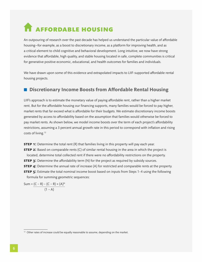
n Discretionary Income Boosts from Affordable Rental Housing
LIIF’s approach is to estimate the monetary value of paying affordable rent, rather than a higher market
rent. But for the affordable housing our financing supports, many families would be forced to pay higher,
market rents that far exceed what is affordable for their budgets. We estimate discretionary income boosts
generated by access to affordability based on the assumption that families would otherwise be forced to
pay market rents. As shown below, we model income boosts over the term of each project’s affordability
restrictions, assuming a 3 percent annual growth rate in this period to correspond with inflation and rising
costs of living.12
step 1: Determine the total rent (R) that families living in this property will pay each year.
step 2: Based on comparable rents (C) of similar rental housing in the area in which the project is
located, determine total collected rent if there were no affordability restrictions on the property.
step 3: Determine the affordability term (N) for the project as required by subsidy sources.
step 4: Determine the annual rate of increase (A) for restricted and comparable rents at the property.
step 5: Estimate the total nominal income boost based on inputs from Steps 1–4 using the following
formula for summing geometric sequences:
Sum = (C – R) – (C – R) × (A)N
(1 – A)
12 Other rates of increase could be equally reasonable to assume, depending on the market.
7
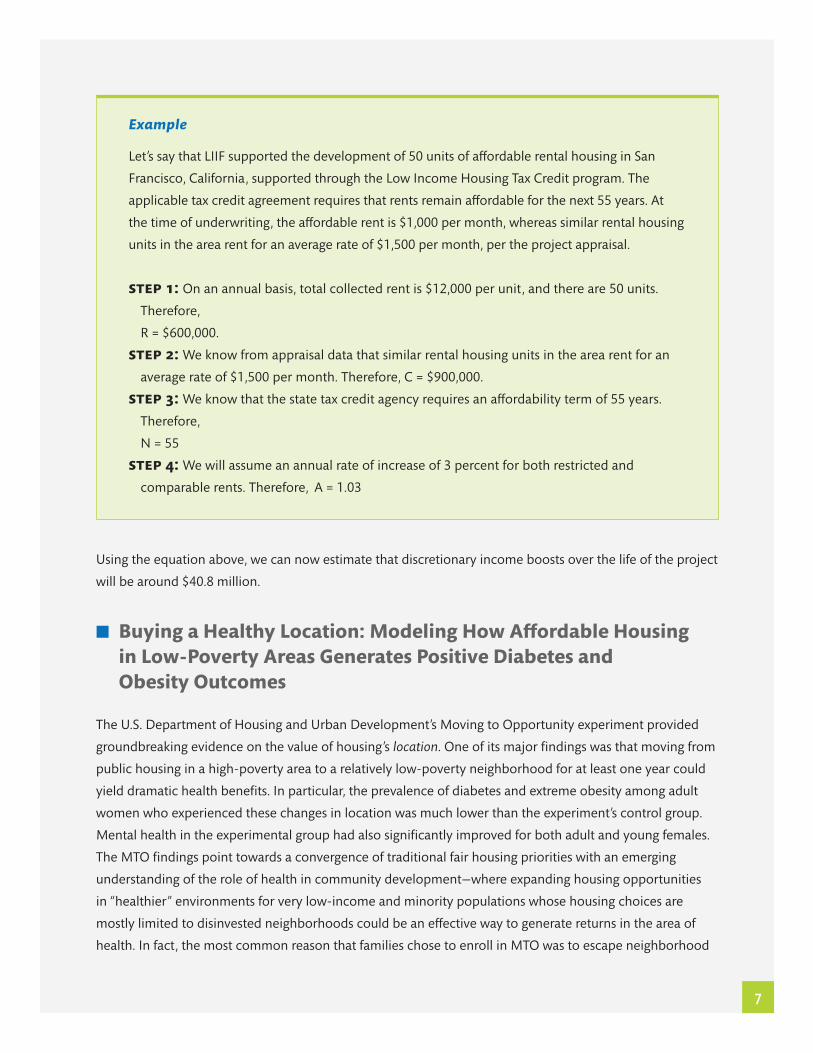
Example
Let’s say that LIIF supported the development of 50 units of affordable rental housing in San
Francisco, California, supported through the Low Income Housing Tax Credit program. The
applicable tax credit agreement requires that rents remain affordable for the next 55 years. At
the time of underwriting, the affordable rent is $1,000 per month, whereas similar rental housing
units in the area rent for an average rate of $1,500 per month, per the project appraisal.
step 1: On an annual basis, total collected rent is $12,000 per unit, and there are 50 units.
Therefore,
R = $600,000.
step 2: We know from appraisal data that similar rental housing units in the area rent for an
average rate of $1,500 per month. Therefore, C = $900,000.
step 3: We know that the state tax credit agency requires an affordability term of 55 years.
Therefore,
N = 55
step 4: We will assume an annual rate of increase of 3 percent for both restricted and
comparable rents. Therefore, A = 1.03
Using the equation above, we can now estimate that discretionary income boosts over the life of the project
will be around $40.8 million.
n Buying a Healthy Location: Modeling How Affordable Housing in Low-Poverty Areas Generates Positive Diabetes and Obesity Outcomes
The U.S. Department of Housing and Urban Development’s Moving to Opportunity experiment provided
groundbreaking evidence on the value of housing’s location. One of its major findings was that moving from
public housing in a high-poverty area to a relatively low-poverty neighborhood for at least one year could
yield dramatic health benefits. In particular, the prevalence of diabetes and extreme obesity among adult
women who experienced these changes in location was much lower than the experiment’s control group.
Mental health in the experimental group had also significantly improved for both adult and young females.
The MTO findings point towards a convergence of traditional fair housing priorities with an emerging
understanding of the role of health in community development—where expanding housing opportunities
in “healthier” environments for very low-income and minority populations whose housing choices are
mostly limited to disinvested neighborhoods could be an effective way to generate returns in the area of
health. In fact, the most common reason that families chose to enroll in MTO was to escape neighborhood
8
violence—a frame of decision-making that HUD planners at the time did not interpret as being related
to health, but which many now recognize as having been a conscious effort by heads-of-household to
“purchase health” for their families in the form of a different location.
Applying the MTO health results to the LIIF portfolio is an imperfect science. For instance, differences
between the two contexts’ design and strength of the “treatment,” as well as population characteristics,
make this extrapolation inexact. One example of such a difference is that families who live in LIIF-supported
units are likely not as high-needs, nor as low-income as the MTO population, nor are their counterfactual
neighborhoods—the places they would live but for access to housing in low-poverty areas—likely as high-
poverty. In other words, the LIIF-supported population might not be as primed to reap positive health
benefits from a change in location.
On the other hand, the unit-based subsidies in low-poverty areas that LIIF supports constitute a stronger
“treatment” than what MTO families experienced, from the perspective of helping them maintain stability
in low-poverty areas and sustain access to whatever benefits they provide (in addition to avoiding exposure
to risks in high poverty areas). MTO families with tenant-based vouchers faced the constant threat—and,
often, reality—of involuntary moves, and they were only required to stay in low-poverty areas for one year.13
Many reverted to higher-poverty areas shortly thereafter—almost never due to a desire to return to their old
neighborhood—which likely reduced the strength and lasting impact of the positive “neighborhood effects”
that MTO was designed to test.
Whatever the complexity and uncertainties around applying the MTO health results to non-MTO
circumstances, data from the experiment do provide a path to make rudimentary estimates of health
improvements from changing neighborhood circumstances. And although census tract poverty rate turned
out to be an inadequate proxy for higher performing schools, MTO evaluators still found that area poverty
had a linear relationship with most of the outcomes they tracked—including health improvements.14
13 The one-year requirement—and, perhaps more importantly, the lack of post-move support or second-move housing search assistance—has prompted some advocates to call the MTO program model a “weak” treatment. See, for example: Tegeler, Philip, and Hankins, Salimah. “Prescription for a New Neighborhood.” Shelterforce, Spring 2012. Website: http://www.shelterforce.org/article/2769/ prescription_for_a_new_neighborhood/ 14 The initial analysis that revealed this linear relationship, later confirmed in follow-up studies, was: Kling JR, Liebman JB, Katz LF. 2007. “Experimental Analysis of Neighborhood Effects.” Econometrica. 75(1): 83-119.
9
In particular, a study by Ludwig et al that focused on physical health impacts for adult women in MTO15
suggests a simple way to estimate changes in diabetes and extreme obesity16 prevalence based on changes
in neighborhood characteristics. The authors’ quasi-experimental instrumental variables analysis of the MTO
data found that a 10 percentage point drop in duration-weighted census tract poverty was associated the
ollowing outcomes:
• A 6.2 percentage point drop in likelihood of class II obesity (BMI ≥ 35)
• A 4.3 percentage point drop in likelihood of class III obesity (BMI ≥ 40)
• A 3.2 percentage point drop in likelihood of diabetes (HbA1c ≥ 6.5%)17
Although other recent MTO studies focused on “high dosage” households that stayed in lower-poverty areas
for longer periods have suggested other positive impacts, such as health improvements and educational
achievement for children,18 we feel that research on MTO sub-group effects is still nascent and not widely
accepted. As such, we only derive impact measures from MTO studies with the strongest statistical power
(such as the Ludwig et al study on adult diabetes and obesity).
Our Approach
Using the Ludwig et al study as a guide and starting point, we can model the health improvements that
LIIF helps generate by providing access to “healthy” communities for low-income families whose housing
choices we assume to be otherwise restricted to higher-poverty areas. It is also worth noting that our
methodology can apply to both new construction and preservation projects, based upon the theory that
low-income families would be displaced to higher-poverty areas were it not for access to subsidized units
in low-poverty areas within the overheated coastal markets where LIIF invests. For preservation projects,
then, our approach to estimating impact could be interpreted as avoided declines in health, rather than
improvements in health.
Which Projects Qualify
Although the study suggests a way to model diabetes and extreme obesity impacts according to any given
duration-weighted change in census tract poverty rate over an equivalent 10-year study period, we believe
it is reasonable to only model improvements generated by LIIF-supported projects in areas that meet the
same threshold that the MTO program model used for identifying low-poverty neighborhoods
15 Ludwig, et al. 2011. “Neighborhoods, Obesity, and Diabetes—A Randomized Social Experiment.” New England Journal of Medicine. 365:1509-1519. October 20.16 Obesity is defined as having Body Mass Index (BMI) of 30 or higher. Obesity ranges above BMI of 35 are called extreme, morbid, or severe. We use the term ‘extreme’ as a catch-all for this sub-group.17 It can be helpful to think of these drops as differences in prevalence between a treatment and control group, whatever changes in prevalence (if any) occurred in either group relative to baseline.18 For example, see: Moulton et al. 2014. “Moving to Opportunity ’s Impact on Health and Well-Being Among High-Dosage Participants.” Housing Policy Debate. Vol 24, No. 2.

10
of “opportunity” to qualify as landing spots for families moving out of public housing—census tract poverty
levels below 10 percent.19
In addition, even though obesity improvements were detected at the MTO interim impacts evaluation, the
MTO data does not tell us when, within the 10-year study period, those positive health outcomes emerged.
As a result, we assume that benefits emerge over a 10-year period in order to correspond with the MTO
study period.
Health Outcomes vs. Health Expenditures
It is worth noting that no existing research can confirm whether MTO families who moved to low-poverty
areas actually generated lower medical expenditures—not to mention a specific dollar reduction—even if
their health improved overall. It is even conceivable that in some cases, moving to a “healthier” area meant
better access to medical care, which might have generated an increase in health costs. Researchers at Johns
Hopkins University have set out to answer these questions by pairing Medicaid and other health care
insurance claims data with MTO data, but results aren’t expected in the near term.
Our approach for now, then, is to base our modeling of reduced expenditures on those physical health
outcomes that demonstrated statistically significant changes—diabetes and extreme obesity improvements—
and on research associated with the incremental increase in medical costs associated with those conditions.
Put differently, we assume that elimination of a medical condition such as diabetes means that the
incremental costs associated with having that condition are also gone.
Families’ Housing Careers
Once we have a list of qualifying projects, we still need to make a few assumptions about families’ “housing
careers” over the hypothesized 10-year period (again, corresponding to the MTO study period) in order
to use the Ludwig et al study and other research on particular medical conditions to model health
improvements and their cost savings.
Each of these assumptions, and our rationale behind them, are explained in detail below. To see how these
assumptions feed into the impact calculation, please jump ahead to the step-by-step calculation in the
following section.
1. Hypothesized counterfactual tract poverty rates for families living in LIIF-supported units in low-poverty
areas—where they would be living but for access to these units.
Although the concentration of low-income housing and those receiving tenant-based rental
assistance in higher poverty areas suggests that the availability of subsidized units in low-poverty
areas could represent an opportunity for low-income families to experience a significant reduction in
19 We will monitor tract poverty rates on an annual basis to ensure that we do not “qualify” projects in areas with rapidly rising poverty rates.
11
neighborhood poverty levels, there is no way for us to know to what extent this takes place in LIIF-
supported units in low-poverty areas—let alone what those reductions might be, on average.
Given this level of uncertainty, we believe it is reasonable to assume a constant counterfactual tract
poverty rate equivalent to the average census tract poverty rate for all housing projects (not to be
confused with housing units) for which LIIF has this data—all projects since 2005, and a handful from
before this time—according to the then-most recent decennial census at the time LIIF helped finance
the project. This average tract poverty rate is approximately 24 percent.
2. How long families who do lease up in LIIF-supported units in low-poverty areas are hypothesized to live in
them before moving out.
It would be overly optimistic to assume that families who live in LIIF-supported housing in low-poverty
areas will stay in these units for entire 10-year periods. Length of tenure is impacted by several factors,
including demographics (e.g., families with children vs. seniors) and income amount. Research on
length of stay in low-income housing programs has shown that, on average, families stay in subsidized
units for several years—for example, one survey found an average of 4.4 years for non-senior units in
LIHTC properties,20 and another analysis of HUD data showed an average of 3.4 years in public housing
for families with children21—but ranges are considerable. To be conservative, we estimate that families
stay in LIIF-assisted low-poverty unit for 4 years.
3. Tract poverty rates for areas where families who lived in LIIF-supported units in low-poverty areas live once
they move out.
We believe it is reasonable to assume that once families move out of their units in low-poverty areas,
they will not be able to find housing in areas with similarly low poverty rates. Housing markets simply
aren’t so kind, and the vast majority of families in LIIF-supported don’t have the benefit of tenant-based
rental assistance that follows them to their next unit (and theoretically expands housing options), as do
families who participate in traditional mobility programs.
However, researchers have found that families that participate in mobility programs and “revert”
back to higher poverty areas often move to neighborhoods with poverty rates that still represent an
improvement on their starting neighborhood (perhaps in an effort to keep some of the benefits of low-
poverty areas, and/or due to newfound market savvy). With this in mind, our model assumes that for
the remainder of the 10-year period where families did not live in low-poverty areas, they lived in an
area with a poverty rate of 15 percent.
20 AARP Public Policy Institute. 2006. “Developing Appropriate Rental Housing for Low-Income Older Persons: A Survey of Section 202 and LIHTC Property Managers.” December.21 Lubell, Jeffrey M., Shroder, Mark, and Steffen, Barry. 2003. “Work Participation and Length of Stay in HUD-Assisted Housing.” U.S. Department of Housing and Urban Development, Office of Policy Development and Research. Cityscape: A Journal of Policy Development and Research. Vol 6, No 2.
12
4. When positive health outcomes first emerge in families’ housing careers, and how long they last.
Unfortunately, even though obesity improvements were detected at the MTO interim impacts
evaluation, the MTO data does not tell us exactly when, over the course of the study period, positive
health outcomes emerged. To be conservative, we model these benefits as appearing at the end of
the 10-year “treatment” period after a family is first hypothesized to have moved from a tract with 24
percent poverty to that particular low-poverty property.
The MTO data also does not include information about whether health benefits were sustained over
time, beyond the point-in-time measurements at the end of the study period. Although we do not have
evidence to suggest whether our rationale is reasonable or not, we assume that for each family that is
hypothesized to experience health benefits from living in LIIF-supported housing in low-poverty areas,
these benefits were sustained for 4 years after the hypothesized 10-year “treatment” period ends (to
correspond with the four years that they lived in the property)..
Prevalence and Costs for Diabetes and Extreme Obesity
Our methodology requires that we have estimates for diabetes and extreme (class II and class III)
obesity costs, and population prevalence for each to serve as baselines and control comparisons for the
hypothesized health improvements among the “treatment” population.
DIABETES PREVALENCE
Some context: diabetes can cause health complications such as heart disease, blindness, kidney failure, and
amputations. It is also the seventh-leading cause of death in the country. Among adults, 90–95 percent of
diagnosed cases of diabetes are type 2 diabetes—also known as adult-onset diabetes—which is associated
with obesity. However, studies have shown that regular physical activity can significantly reduce the risk of
developing type 2 diabetes.22
In 2012, 12.3 percent of adults 20 years and older were estimated to have diabetes (both diagnosed and
undiagnosed),23 although this figure is significantly higher for minority populations that are more likely to
be low-income, and thus overrepresented in LIIF-supported housing—for example, 18.7 percent of non-
Hispanic blacks have diabetes,24 and this figure was 20 percent of the MTO control group. In addition,
populations with lower socioeconomic status have also shown to have higher rates of diabetes.25
22 Centers for Disease Control and Prevention. 2014. “Basics about Diabetes.” Website: http://www.cdc.gov/diabetes/consumer/learn.htm. Last reviewed (by the CDC) on March 7, 2014.23 Centers for Disease Control and Prevention, 2014. “National Diabetes Statistics Report, 2014.” Website: http://www.cdc.gov/diabetes/pubs/statsreport14/national-diabetes-report-web.pdf. 24 Centers for Disease Control and Prevention. 2011. “National Diabetes Fact Sheet, 2011.” Website: http://www.cdc.gov/diabetes/pubs/pdf/ndfs_2011.pdf. Figure is both diagnosed and undiagnosed cases.25 See, for example: Baumann et al. 2002. “Clinical Outcomes for Low-Income Adults with Hypertension and Diabetes.” Nursing Research. Vol. 51, No. 3. May/June. Also note that diabetes prevalence is higher among those receiving Medicare and Medicaid, especially for “dual eligibles.”
13
Diabetes prevalence is also increasing at a rapid pace, and has been for some time. The rate has tripled
since 1980, and researchers have projected dramatic increases in the coming decades. UnitedHealth
Group, a health care company (that has begun to invest in low-income housing as an approach to reduce
medical costs), projects that the prevalence of both diagnosed and undiagnosed cases will be 15 percent
by 2020.26 Looking even longer-term, the Centers for Disease Control and Prevention (CDC) projects that
between 20 and 33 percent of the U.S. population will have diabetes by 2050.27 A recent study projected
that the lifetime risk of being diagnosed with diabetes for those born between 2000 and 2011 is around
40 percent, and these figures are even higher—over 50 percent—for Hispanic men and women, and non-
Hispanic black women.28
Considering the higher incidence of diabetes both lower-income and minority populations when compared
to the rest of the country, and the projected increases in diabetes overall, we conservatively assume that
15 percent of adults in LIIF-supported housing have diabetes, either diagnosed or undiagnosed (before
experiencing the “treatment” of living in a low-poverty area).
DIABETES COSTS
Our approach to monetizing the cost of diabetes does not account for indirect costs (e.g., disability, lost
work productivity, premature death), but rather on shorter-term savings in annual medical expenditures. On
average, people diagnosed with diabetes have annual medical expenditures that are approximately 2.3 times
higher than what they would be in the absence of diabetes; in 2012 dollars, the average per capita annual
medical costs attributable to diabetes alone was $7,900. This figure is higher for minority populations that are
likely overrepresented in LIIF-supported housing—for example, the figure is $9,540 for non-Hispanic blacks.29
Landing somewhere in the middle, we assume that, for the estimated 15 percent of adults who live in LIIF-
supported housing and have diabetes, their annual medical expenditures associated with the condition
are $8,500. As previously noted, our approach to modeling cost reductions assumes that elimination of the
disease is associated with savings equivalent to this amount. In addition, we assume a 6 percent annual
nominal growth rate in savings due to rising medical costs (the same rate of increase that the Centers for
Medicare & Medicaid Services projects for the next 10 years).30
26 UnitedHealth Center for Health Reform & Modernization, 2010. “The United States of Diabetes: Challenges and Opportunities in the decade ahead.” Working Paper 5. November.27 Boyle, et al. 2010. “Projection of the year 2050 Burden of Diabetes in the US Adult Population: Dynamic Modeling of Incidence, Mortality, and Prediabetes Prevalence.” Population Health Metrics. 8:29. 28 Gregg, et al. 2014. “Trends in lifetime risk and years of life lost due to diabetes in the USA, 1985–2011: a modelling study.” The Lancet Diabetes & Endicronology, Early Online Publication, 13 August.29 American Diabetes Association. 2013. “Economic Costs of Diabetes in the U.S. in 2012.” Website: http://care.diabetesjournals.org/content/early/2013/03/05/dc12-2625.full.pdf+html 30 Sisco, et al. 2014. “National Health Expenditure Projections, 2013–23: Faster Growth Expected with Expanded Coverage and Improving Economy.” Health Affairs. Vol. 33, No. 10.

14
EXTREME OBESITY PREVALENCE
Similar to diabetes, obesity is associated with premature death and a range of other medical complications.
For example, BMI of 30–35 is associated with a lifespan reduction of 3 years, and BMI of 40–50 is associated
with reduced life expectancy of 10 years.31 As noted earlier in this document, obesity is a risk factor for
diabetes, and the two conditions are considered comorbidities.
As of 2010, the prevalence of class II and class III obesity for the total U.S. adult population 20 years and
older was estimated to be 15.4 percent and 6.3 percent, respectively.32 However, similar to diabetes (for
which obesity is a risk factor), prevalence of extreme obesity in low-income and minority populations is
higher than general population averages.
For example, the 2010 prevalence of class II and class III obesity for non-Hispanic blacks was 26 percent
and 13.1 percent, respectively; the rates for women in this sub-group was even higher, at 30.9 percent and
18 percent.33 Further, a CDC study of obesity trends from 2005-2008 found that obesity was 13 percentage
points higher for low-income non-Hispanic black women, when compared to all low-income women. The
gap between low-income people those with higher income was also substantial across nearly all racial/
ethnic and gender breakdowns.
Extreme obesity is also similar to diabetes in that it is rapidly increasing, and is projected to impact a
growing percentage of the population. Class III obesity (BMI of 40 and above) is the fastest growing category
of obesity;34 between 2000 and 2010, its prevalence increased by 70 percent, and the rate of increase
for BMI of 50 and above was even faster.35 Looking into the not-too-distant future, a National Bureau of
Economic Research study projects that in 2020, class II and class III obesity will impact 21 percent and 14
percent of the population, respectively; for women, these figures are 25 percent and 18 percent.36
Considering the higher prevalence of extreme obesity in both lower-income and minority populations when
compared to the rest of the country, and the projected rapid increases in the outer ranges of obesity, we
conservatively assume that the prevalence of class II and class III obesity in adults in LIIF-supported housing is
20 percent and 12 percent, respectively (before experiencing the “treatment” of living in a low-poverty area).
31 Whitlock, et al. 2009. “Body-mass index and cause-specific mortality in 900,000 adults: collaborative analyses of 57 prospective studies.” Lancet. March 28. 373 (9669):1083-96.32 Flegal, et al. 2012. “Prevalence of Obesity and Trends in the Distribution of Body Mass Index Among US Adults, 1999–2010.” Journal of the American Medical Association. February 1. Vol 307, No. 5. 33 Flegal, et al. 2012. 34 Grieve, E., Fenwick, E., Yang, H.-C. and Lean, M. 2013. “The disproportionate economic burden associated with severe and complicated obesity: a systematic review.” Obesity Reviews. Nov;14(11):883-94.35 Sturm, Roland, and Hattori, AIko. 2013. “Morbid Obesity Rates Continue to Rise Rapidly in the US.” International Journal of Obesity. June. Vol 37, No. 6.36 Ruhm, Christopher. 2007. “Current and Future Prevalence of Obesity and Severe Obesity in the United States.” National Bureau of Economic Research Working Paper Series. Working Paper 13181.
15
As previously noted, obesity is a comorbidity with diabetes. Current research estimates that 15 percent of
those with class II obesity and 26 percent of those with class III obesity have diabetes.37 For the purpose
of not double-counting, we only calculate hypothesized obesity-related medical cost reductions for the
percentage of adults living in LIIF-supported housing in low-income areas who we estimate to have class II
and III obesity, but not diabetes. Specifically:
• We assume that only 85 percent of hypothesized changes in class II obesity prevalence—and cost savings—
resulting from the “treatment” of living in low-poverty neighborhoods will be among those who had
previously had class II obesity without diabetes.
• We assume that only 74 percent of hypothesized changes in class III obesity prevalence—and cost
savings—resulting from the “treatment” of living in low-poverty neighborhoods will be among those who
had previously had class III obesity without diabetes.
EXTREME OBESITY COSTS
Similar to our approach to diabetes, our approach to monetizing improvements in extreme obesity
prevalence does not account for potential longer lifespans, but instead on shorter-term savings in annual
medical expenditures. A systematic review of studies on the direct medical costs of obesity estimated that,
based on the highest quality and most universally applicable studies available, the per-person annual
medical costs of being obese was $1,723 in 2008 dollars ($1891 in 2014 dollars), and that the costs of
having class III obesity was $3,012 in 2008 dollars ($3,306 in 2014 dollars).38 There do not appear to be
good estimates for the cost of class II obesity in particular, although it is reasonable to assume that the costs
associated with this condition would be higher than for all people with BMI of 30 and up, and lower than
the figure for those with class III obesity.
Based on available research, we assume that, for those adults living in LIIF-supported housing who we
estimate to have class II and III obesity, their annual medical expenditures associated with these two
conditions are $2,000 and $3,300, respectively. As previously noted, our approach to modeling cost
reductions assumes that elimination of these conditions is associated with savings equivalent to these
amounts. Again, we assume a 6 percent annual nominal growth rate in savings due to rising medical costs.39
37 Mokdad et al. 2003. “Prevalence of Obesity, Diabetes, and Obesity-Related Health Risk Factors, 2001.” Journal of the American Medical Association. Vol 289, No. 1. 38 Tsai, et al. 2011. “Direct medical cost of overweight and obesity in the United States: a quantitative systematic review.” Obesity Review. January. Vol 12, Issue 1. 50-61.39 Centers for Medicare & Medicaid Services, 2014. “Press Release: Number of Uninsured Projected to Decrease, Faster Health Expenditure Growth Expected as Coverage Expands and the Economy Improves, Actuary Reports.” September 3.
16
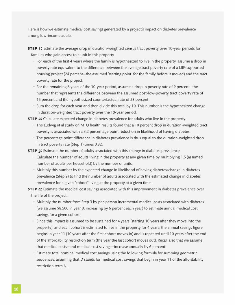
Here is how we estimate medical cost savings generated by a project’s impact on diabetes prevalence
among low-income adults:
step 1: Estimate the average drop in duration-weighted census tract poverty over 10-year periods for
families who gain access to a unit in this property.
• For each of the first 4 years where the family is hypothesized to live in the property, assume a drop in
poverty rate equivalent to the difference between the average tract poverty rate of a LIIF-supported
housing project (24 percent—the assumed ‘starting point’ for the family before it moved) and the tract
poverty rate for the project.
• For the remaining 6 years of the 10-year period, assume a drop in poverty rate of 9 percent—the
number that represents the difference between the assumed post-low-poverty tract poverty rate of
15 percent and the hypothesized counterfactual rate of 23 percent.
• Sum the drop for each year and then divide this total by 10. This number is the hypothesized change
in duration-weighted tract poverty over the 10-year period.
step 2: Calculate expected change in diabetes prevalence for adults who live in the property.
• The Ludwig et al study on MTO health results found that a 10 percent drop in duration-weighted tract
poverty is associated with a 3.2 percentage point reduction in likelihood of having diabetes.
• The percentage point difference in diabetes prevalence is thus equal to the duration-weighted drop
in tract poverty rate (Step 1) times 0.32.
step 3: Estimate the number of adults associated with this change in diabetes prevalence.
• Calculate the number of adults living in the property at any given time by multiplying 1.5 (assumed
number of adults per household) by the number of units.
• Multiply this number by the expected change in likelihood of having diabetes/change in diabetes
prevalence (Step 2) to find the number of adults associated with the estimated change in diabetes
prevalence for a given “cohort” living at the property at a given time.
step 4: Estimate the medical cost savings associated with this improvement in diabetes prevalence over
the life of the project.
• Multiply the number from Step 3 by per-person incremental medical costs associated with diabetes
(we assume $8,500 in year 0, increasing by 6 percent each year) to estimate annual medical cost
savings for a given cohort.
• Since this impact is assumed to be sustained for 4 years (starting 10 years after they move into the
property), and each cohort is estimated to live in the property for 4 years, the annual savings figure
begins in year 11 (10 years after the first cohort moves in) and is repeated until 10 years after the end
of the affordability restriction term (the year the last cohort moves out). Recall also that we assume
that medical costs—and medical cost savings—increase annually by 6 percent.
• Estimate total nominal medical cost savings using the following formula for summing geometric
sequences, assuming that D stands for medical cost savings that begin in year 11 of the affordability
restriction term N.
17
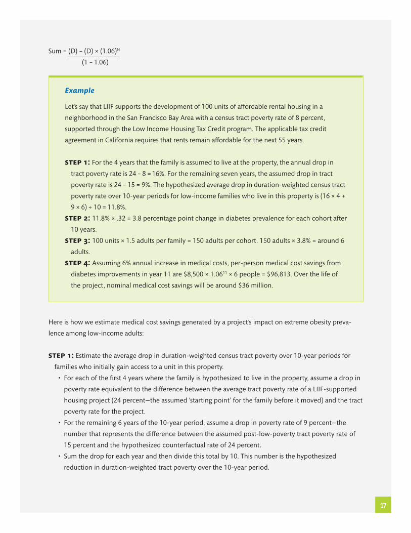
Sum = (D) – (D) × (1.06)N
(1 – 1.06)
Example
Let’s say that LIIF supports the development of 100 units of affordable rental housing in a
neighborhood in the San Francisco Bay Area with a census tract poverty rate of 8 percent,
supported through the Low Income Housing Tax Credit program. The applicable tax credit
agreement in California requires that rents remain affordable for the next 55 years.
step 1: For the 4 years that the family is assumed to live at the property, the annual drop in
tract poverty rate is 24 – 8 = 16%. For the remaining seven years, the assumed drop in tract
poverty rate is 24 – 15 = 9%. The hypothesized average drop in duration-weighted census tract
poverty rate over 10-year periods for low-income families who live in this property is (16 × 4 +
9 × 6) ÷ 10 = 11.8%.
step 2: 11.8% × .32 = 3.8 percentage point change in diabetes prevalence for each cohort after
10 years.
step 3: 100 units × 1.5 adults per family = 150 adults per cohort. 150 adults × 3.8% = around 6
adults.
step 4: Assuming 6% annual increase in medical costs, per-person medical cost savings from
diabetes improvements in year 11 are $8,500 × 1.0611 × 6 people = $96,813. Over the life of
the project, nominal medical cost savings will be around $36 million.
Here is how we estimate medical cost savings generated by a project’s impact on extreme obesity preva-
lence among low-income adults:
step 1: Estimate the average drop in duration-weighted census tract poverty over 10-year periods for
families who initially gain access to a unit in this property.
• For each of the first 4 years where the family is hypothesized to live in the property, assume a drop in
poverty rate equivalent to the difference between the average tract poverty rate of a LIIF-supported
housing project (24 percent—the assumed ‘starting point’ for the family before it moved) and the tract
poverty rate for the project.
• For the remaining 6 years of the 10-year period, assume a drop in poverty rate of 9 percent—the
number that represents the difference between the assumed post-low-poverty tract poverty rate of
15 percent and the hypothesized counterfactual rate of 24 percent.
• Sum the drop for each year and then divide this total by 10. This number is the hypothesized
reduction in duration-weighted tract poverty over the 10-year period.

18
step 2: Calculate expected change in class II and III obesity prevalence for adults who live in the property.
• The Ludwig et al study on MTO health results found that a 10 percent drop in duration-weighted tract
poverty is associated with 6.2 and 4.3 percentage point reduction in likelihood of having class II and
III obesity, respectively.
• The percentage point difference in class II and III obesity prevalence is thus equal to the duration-
weighted drop in tract poverty rate (Step 1) times 0.62 and 0.43, respectively.
step 3: Estimate the number of adults associated with this change in class II and III obesity prevalence.
• Calculate the number of adults living in the property at any given time by multiplying 1.5 (assumed
number of adults per household) by the number of units.
• Multiply this number by the expected change in likelihood of having class II and III obesity/change
in extreme obesity prevalence (Step 2) to find the number of adults associated with the estimated
changes in extreme obesity prevalence for a given “cohort” living at the property at a given time.
• Then, in order not to double-count with diabetes improvements, multiply the class II obesity number
from the previous step by .85 (to reflect the assumption that 15% will also have diabetes) and the
number for class III obesity by .74 (to reflect the assumption that 26% will also have diabetes).
step 4: Estimate the medical cost savings associated with this improvement in diabetes prevalence over
the life of the project.
• Multiply the numbers from Step 3 by per-person incremental medical costs associated with class II
and III obesity (we assume $2,000 and $3,300 in year 0, respectively, increasing by 6 percent each
year) to estimate annual medical cost savings for a given cohort.
• Since this impact is assumed to be sustained for 4 years (starting 10 years after they move into the
property), and each cohort is estimated to live in the property for 4 years, the annual savings figure
begins in year 11 (10 years after the first cohort moves in) and is repeated until 10 years after the end
of the affordability restriction term (the year the last cohort moves out). Recall also that we assume
that medical costs—and medical cost savings—increase annually by 6 percent.
• Estimate total anticipated medical cost savings using the following formula for summing geometric
sequences, assuming that O stands for medical cost savings that begin in year 11 of the affordability
restriction term N.
Sum = (O) – (O) × (1.06)N
(1 – 1.06)
19
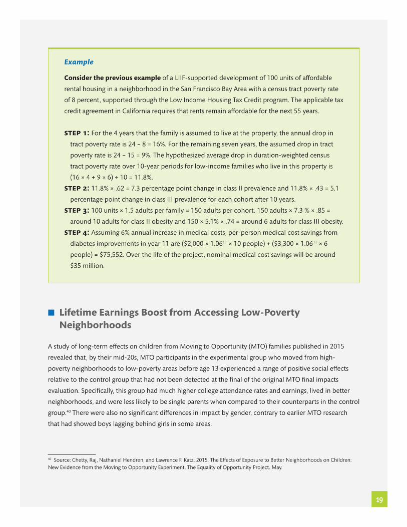
Example
Consider the previous example of a LIIF-supported development of 100 units of affordable
rental housing in a neighborhood in the San Francisco Bay Area with a census tract poverty rate
of 8 percent, supported through the Low Income Housing Tax Credit program. The applicable tax
credit agreement in California requires that rents remain affordable for the next 55 years.
step 1: For the 4 years that the family is assumed to live at the property, the annual drop in
tract poverty rate is 24 – 8 = 16%. For the remaining seven years, the assumed drop in tract
poverty rate is 24 – 15 = 9%. The hypothesized average drop in duration-weighted census
tract poverty rate over 10-year periods for low-income families who live in this property is
(16 × 4 + 9 × 6) ÷ 10 = 11.8%.
step 2: 11.8% × .62 = 7.3 percentage point change in class II prevalence and 11.8% × .43 = 5.1
percentage point change in class III prevalence for each cohort after 10 years.
step 3: 100 units × 1.5 adults per family = 150 adults per cohort. 150 adults × 7.3 % × .85 =
around 10 adults for class II obesity and 150 × 5.1% × .74 = around 6 adults for class III obesity.
step 4: Assuming 6% annual increase in medical costs, per-person medical cost savings from
diabetes improvements in year 11 are ($2,000 × 1.0611 × 10 people) + ($3,300 × 1.0611 × 6
people) = $75,552. Over the life of the project, nominal medical cost savings will be around
$35 million.
n Lifetime Earnings Boost from Accessing Low-Poverty Neighborhoods
A study of long-term effects on children from Moving to Opportunity (MTO) families published in 2015
revealed that, by their mid-20s, MTO participants in the experimental group who moved from high-
poverty neighborhoods to low-poverty areas before age 13 experienced a range of positive social effects
relative to the control group that had not been detected at the final of the original MTO final impacts
evaluation. Specifically, this group had much higher college attendance rates and earnings, lived in better
neighborhoods, and were less likely to be single parents when compared to their counterparts in the control
group.40 There were also no significant differences in impact by gender, contrary to earlier MTO research
that had showed boys lagging behind girls in some areas.
40 Source: Chetty, Raj, Nathaniel Hendren, and Lawrence F. Katz. 2015. The Effects of Exposure to Better Neighborhoods on Children: New Evidence from the Moving to Opportunity Experiment. The Equality of Opportunity Project. May.
20
We use this study’s finding on long-term earnings increases to estimate the same kind of impact on children
who gain access to LIIF-supported affordable housing projects in low-poverty neighborhoods. Translating
this research to LIIF projects involves a similar approach—described below—as the one used in the “Buying
a Healthy Location” metric described earlier in this document, which draws from a separate study on MTO
that focuses on adult metabolic health impacts.
Magnitude of Earnings Increase
Among MTO children group who moved before age 13, the experimental group saw an earnings increase
of 31 percent, on average, when compared to the control group. Children under age 13 in the MTO Section
8 voucher group—whose families were offered a housing voucher to move out of public housing, but did
not receive mobility services and were not required to move to low-poverty neighborhoods—experienced a
15 percent earnings increase. This finding is consistent with the fact that families in this group experienced
about half the reduction of neighborhood poverty when compared to the experimental group.
The typical percentage point drop in neighborhood poverty rates that we estimate families living in LIIF-
supported affordable housing in low-poverty areas experience over time, compared to where they would
have lived were it not having gained access to this housing (as described in in the “Families’ Housing
Careers” section of the “Buying a Healthy Location” metric earlier in this document), is about the same
as what families in the MTO Section 8 group experienced relative to that experiment’s control group. For
this reason, we assume that children under age 13 who live in LIIF-supported properties in low-poverty
areas experience same level of lifetime earnings increase as for the MTO Section 8 group—approximately
$150,000 in real dollars, or around 15 percent higher than the control—when compared to children of
similar age who we hypothesize would have otherwise remained in relatively higher-poverty areas. We
use Social Security Administration (SSA) earnings projections for children graduating high school today to
estimate when this impact appears over time.41
How many Children Experience this Impact?
Since this metric estimates long-term income impacts for children, it only applies to units intended for
households with children—as opposed to those which are targeted to populations without children such as
supportive housing units for the homeless.
41 Office of Retirement Policy, Social Security Administration. MINT 7 projections.

21
Within each family-oriented unit, we conservatively assume one child per bedroom beyond the first
bedroom, which we assume is for the parent(s)/guardian(s) in the household. For example, in a given
5-bedroom apartment we would assume four total children in the four bedrooms beyond the first bedroom.
Since three quarters of poor children below age 18 in the United States under age 13,42 we would assume
that—at the time a family moves into the unit—three of the four children in this household are below age 13,
and would thus experience positive long-term earnings from accessing a low-poverty neighborhood.43
Similar to our approach in developing the “Buying a Healthy Location” metric described earlier in this
document, we assume that families live in the property for four years (see that section for further rationale on
why we choose this time “dose”). As such, there is a new set of families that moves in every four years—each
of which contains a new cohort of children who we assume will experience long-term earnings increases.
With these assumptions in place, here is how we estimate lifetime earnings impacts for children from low-
income families who move to affordable housing in low-poverty neighborhoods:
step 1: Estimate the number of children who will experience an earnings increase.
• Multiply the number of family-targeted units in the property by 1.5 to estimate the number of
children under age 13 in each cohort.
• To calculate the number of “cohorts” of children who will move to the property, divide the project’s
affordability term in years by four (the number of years each child is hypothesized to live in this
property).
• Multiply the results of the first two steps to estimate the total number of children who will experience
earnings increases, over the entire affordability term of the project.
step 2: Estimate the total amount of earnings impact.
• Assume a lifetime earnings impact of $150,000, in real dollars, per child who moves into the property
before age 13.
• Adjust earnings estimates for time value of money—accounting for the fact that earnings do not begin
until these children are 18 years old,44 and that each new cohort moves into the property when the
previous cohort moves out.
42 2009-2013 American Community Survey 5-Year Estimates, Table V17001: Poverty Status in the Past 12 months by Sex by Age.43 To simplify the user experience in the online version of the Social Impact Calculator (www.liifund.org/calculator), we assume an average apartment size of three bedrooms. Per our methodology, a three-bedroom apartment translates to two children per household, 1.5 of which would be under age 13 at the time of the move.44 Per the MTO study, we assume that children who move before age 13 are, on average, 8 years old at the time of the move (or 10 years before they will begin earning an income).
22
Example
Let’s say that LIIF supports the development of a 30-unit affordable housing project in a low-
poverty neighborhood that is entirely comprised of three-bedroom units for families with
children. To keep it simple, let’s assume an affordability term of four years (the amount of time
each cohort of families is assumed to live in the property before moving out).
step 1: We assume that each three-bedroom unit has two children, and three quarters of these
children are below age 13. There are 30 total units, so the number of children in each cohort is
30 * 2 * 0.75 = 45. Since the affordability term is only four years, there is only one cohort.
step 2: Each of the 45 children who move to the property before age 13 will experience a
$150,000 earnings impact, in real 2015 dollars. 45 * $150,000 = $6.75 million in 2015 dollars.
If the children move into the property in 2015, we assume that they will begin earning income ten years
later, when they are 18 years old. Adjusting for an inflation rate of 2.2 percent,45 the total lifetime earnings
increase generated by the project is $8.39 million in 2025 dollars.46
n Affordable Housing as a Remedy for Food Insecurity
Children who do not have adequate nutrition are less healthy, suffer developmental impairments, and have
lower educational achievement.47 Recent studies have begun to uncover a strong correlation between
housing costs and food insecurity.48 To estimate the impact of LIIF-supported housing subsidies on food
expenditures, we draw from Bureau of Labors Statistics Consumer Expenditure Survey (CES) data, reported
in the “State of the Nation’s Housing by the Joint Center for Housing Studies of Harvard University. This
report shows that families in the bottom expenditure quartile (a very conservative proxy for low-income)
who live in housing that is affordable to them spend significantly more—around $123 per month more for
families with children, and around $88 more for all renters—on food when compared to their counterparts
45 This is the rate that the SSA uses in its projections, per LIIF tabulation of the following source: Office of Retirement Policy, Social Security Administration. MINT 7 projections.46 The unadjusted, nominal figure is higher. Based on our tabulation of the SSA projections, we estimate that $150,000 in real, discounted dollars translates to around $325,000 in nominal, unadjusted dollars. See the online version of the Social Impact Calculator and the Excel download available on that website to adjust for different social discount rates.47 Cook, John, and Karen Jeng. 2009. “Child Food Insecurity: The Economic Impact on our Nation. A report on research on the impact of food insecurity and hunger on child health, growth and development commissioned by Feeding America and the ConAgra Foods Foundation.”48 See, for example: Fletcher, et al. 2009. “Assessing the effect of changes in housing costs on food insecurity.” Journal of Children and Poverty: Vol. 15, No. 2, 79-93.
23
who are more burdened by housing costs.49 As shown below, we model increased food expenditures over
the term of each project’s affordability restrictions, assuming a 3 percent annual growth rate in this period to
correspond with inflation and rising costs of living.50
step 1: Determine the number of family-oriented (F) and elderly or homeless-oriented (E) affordable
units restricted to low- and very low-income households in a given housing project. Assume monthly
per-F increase in food expenditures of $123, and monthly per-E increased in food expenditures of $88.
step 2: Determine increases in food expenditures (M) in the first year of operation for the project using
the following formula: M = (F × $123 × 12) + (E × $88 × 12).
step 3: Determine the affordability term (N) for the project as required by subsidy sources.
step 4: Determine the annual rate of increase (A) to correspond with inflation and rising cost of living.
estimate the total anticipated income boosts based on inputs from Steps 1–4 using the following
formula for summing geometric sequences:
Sum = (M) – (M) × (A)N
(1 – A)
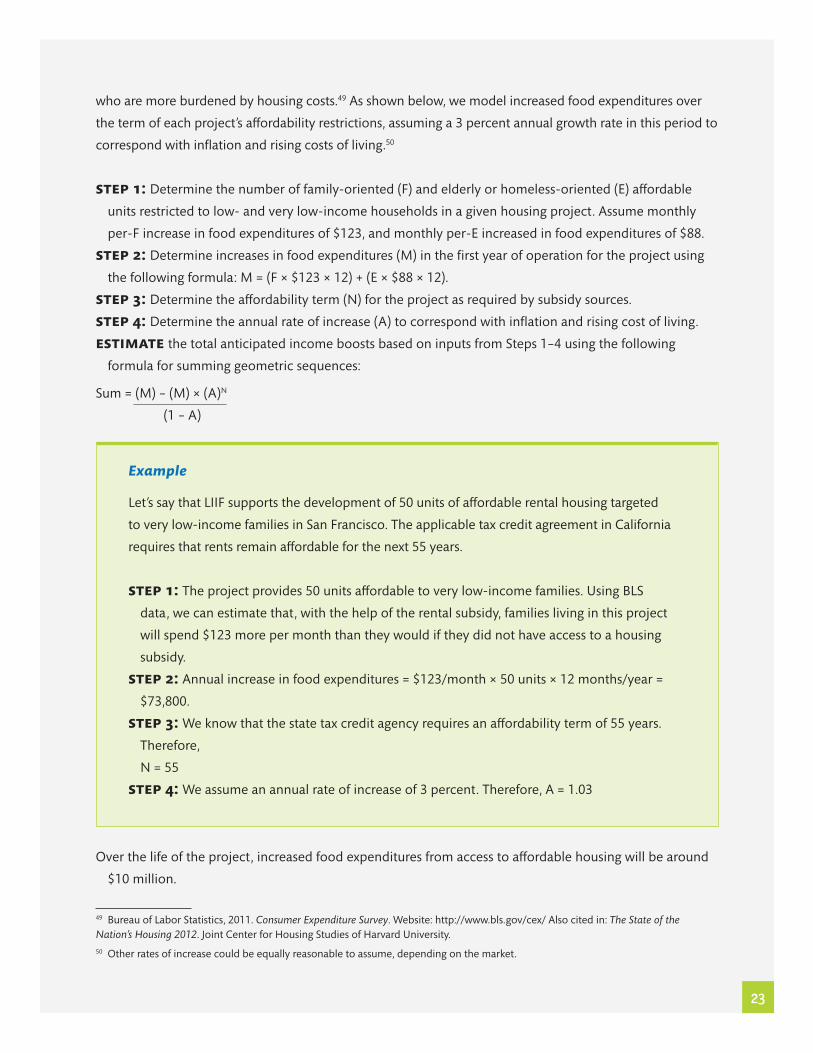
Example
Let’s say that LIIF supports the development of 50 units of affordable rental housing targeted
to very low-income families in San Francisco. The applicable tax credit agreement in California
requires that rents remain affordable for the next 55 years.
step 1: The project provides 50 units affordable to very low-income families. Using BLS
data, we can estimate that, with the help of the rental subsidy, families living in this project
will spend $123 more per month than they would if they did not have access to a housing
subsidy.
step 2: Annual increase in food expenditures = $123/month × 50 units × 12 months/year =
$73,800.
step 3: We know that the state tax credit agency requires an affordability term of 55 years.
Therefore,
N = 55
step 4: We assume an annual rate of increase of 3 percent. Therefore, A = 1.03
Over the life of the project, increased food expenditures from access to affordable housing will be around
$10 million.
49 Bureau of Labor Statistics, 2011. Consumer Expenditure Survey. Website: http://www.bls.gov/cex/ Also cited in: The State of the Nation’s Housing 2012. Joint Center for Housing Studies of Harvard University.50 Other rates of increase could be equally reasonable to assume, depending on the market.

24
n Housing as a Vaccine: Improved Health Outcomes and Medical Cost Savings from Permanent Supportive Housing for the Homeless
Thanks to solid research over the past decade, we can now make reasonable estimates of the medical
cost savings generated by LIIF-supported permanent supportive affordable housing projects. Permanent
supportive housing is an effective strategy for improving positive life outcomes for the chronically
homeless—particularly those with chronic and complex illnesses—which in turn lead to significant public
cost savings, the majority of which are related to reductions in health services.
We draw from the from a 2009 study51 by the Economic Roundtable, based on the quality of the data
available to the authors, the comprehensiveness (across multiple risk factors such as mental health status,
substance abuse problems, and HIV/AIDS) and size of the study population, and the fact that its savings figure
falls somewhere in the middle of the ranges in medical cost savings quoted in other studies.52 As such, it
seemed to be a reasonable but conservative estimate to apply to the LIIF portfolio of permanent supportive
housing projects. The study specifically found that monthly cost savings to public agencies (e.g., County
health services outpatient clinics) and agency sub-departments (e.g., corrections medical services)53 providing
physical and mental health services were $1,853 per month, or $22,242 per year, for those chronically
homeless in permanently supportive housing, compared to those who were not. As shown below, we use this
figure to calculate medical cost savings over the course of a given project’s affordability restriction term. In
addition, we assume a 6 percent annual nominal growth rate in savings due to rising medical costs (the same
rate of increase that the Centers for Medicare & Medicaid Services projects for the next 10 years).54
step 1: Determine medical cost savings (M) from permanent supportive housing in the first year of
operation for the project by multiplying the number of permanent supportive units for the homeless
(assume one person per household in most cases) by the assumed annual per-person medical cost
savings of $22,242.
step 2: Determine the affordability term (N) for the project as required by subsidy sources.
step 3: Determine the annual rate of increase (A) in medical costs.
step 4: Estimate the total anticipated income boosts based on inputs from Steps 1–4 using the following
formula for summing geometric sequences:
51 Economic Roundtable. 2009. “Where We Sleep: Costs when Homeless and Housed in Los Angeles.” 52 See, for example: Culhane, et al. 2002. “Public Service Reductions Associated with Placement of Homeless Persons with Severe Mental Illnesses in Supportive Housing.” Housing Policy Debate. Vol 13, Issue 1. And Larimer, et al. 2009. “Health Care and Public Service Use and Costs Before and After Provision of Housing for Chronically Homeless Persons with Severe Alcohol Problems.” Journal of the American Medical Association. Vol 301, No 13.53 A nominal percentage of health-related costs for this population (2–3 percent) was tracked to private hospitals.54 Centers for Medicare & Medicaid Services, 2014. “Press Release: Number of Uninsured Projected to Decrease, Faster Health Expenditure Growth Expected as Coverage Expands and the Economy Improves, Actuary Reports.” September 3.
25
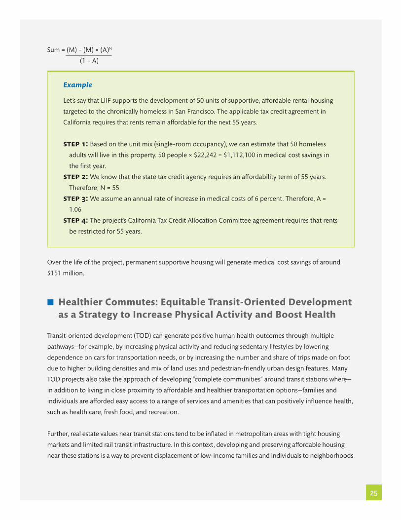
Sum = (M) – (M) × (A)N
(1 – A)
Example
Let’s say that LIIF supports the development of 50 units of supportive, affordable rental housing
targeted to the chronically homeless in San Francisco. The applicable tax credit agreement in
California requires that rents remain affordable for the next 55 years.
step 1: Based on the unit mix (single-room occupancy), we can estimate that 50 homeless
adults will live in this property. 50 people × $22,242 = $1,112,100 in medical cost savings in
the first year.
step 2: We know that the state tax credit agency requires an affordability term of 55 years.
Therefore, N = 55
step 3: We assume an annual rate of increase in medical costs of 6 percent. Therefore, A =
1.06
step 4: The project’s California Tax Credit Allocation Committee agreement requires that rents
be restricted for 55 years.
Over the life of the project, permanent supportive housing will generate medical cost savings of around
$151 million.
n Healthier Commutes: Equitable Transit-Oriented Development as a Strategy to Increase Physical Activity and Boost Health
Transit-oriented development (TOD) can generate positive human health outcomes through multiple
pathways—for example, by increasing physical activity and reducing sedentary lifestyles by lowering
dependence on cars for transportation needs, or by increasing the number and share of trips made on foot
due to higher building densities and mix of land uses and pedestrian-friendly urban design features. Many
TOD projects also take the approach of developing “complete communities” around transit stations where—
in addition to living in close proximity to affordable and healthier transportation options—families and
individuals are afforded easy access to a range of services and amenities that can positively influence health,
such as health care, fresh food, and recreation.
Further, real estate values near transit stations tend to be inflated in metropolitan areas with tight housing
markets and limited rail transit infrastructure. In this context, developing and preserving affordable housing
near these stations is a way to prevent displacement of low-income families and individuals to neighborhoods
26
that are underserved by transit, where they will be unable to benefit from the particular health benefits of
TOD. As such, we believe equitable transit-oriented development—which incorporates housing and services
targeted to lower- and moderate-income households—to be a critical strategy for addressing health disparities
between socioeconomic and racial/ethnic groups living in the same metropolitan regions.
The evidence directly linking TOD to health improvements is, in the current moment, strongly suggestive—
particularly in the area of increasing physical activity—but still limited. For example, studies have revealed
correlations between neighborhood walkability indexes and a range of health outcomes,55 but most
research in this area is not experimental in nature, nor is it easily extrapolated to the LIIF context. However,
a 2010 pre-post longitudinal study of people living near the South Corridor Light Rail line in Charlotte,
North Carolina (before and after it became operational—setting the stage for a “natural experiment”),
provides the first experimental evidence demonstrating that increasing access to transit can mitigate some
environmental barriers to daily physical activity, and generate reductions in body mass index and obesity.
In particular, the study finds that, after adjusting for “treatment” and “control” group characteristics, taking
light rail to work on a daily basis was associated with an average drop in body mass index (BMI) of 1.18—
equivalent to 6.45 pounds for a person whose height is five feet, five inches—12–18 months after follow-up,
and 81 percent of participants reduced their odds of becoming obese during this period.56
If we make a few assumptions, we can apply this study’s findings to LIIF-supported equitable TOD contexts
to give a rough estimate of these projects’ short-term health impacts specifically due to their proximity to
transit. In particular, we need to decide: 1) which projects or units qualify; 2) what percentage of individuals
we hypothesize experience similar health benefits to those in the Charlotte study; 3) the period of impact
for these benefits; and 4) how to monetize these benefits. Our rationale behind each of these assumptions is
provided below:
Which Projects Qualify?
We can only defensibly extrapolate the findings from the Charlotte study to LIIF-supported equitable
TOD projects in markets where access to regionally serving transit is similarly limited—meaning that their
counterfactual housing locations would not likely be transit-accessible.
To this end, we only assume health impacts for LIIF-supported affordable housing projects that obtain
financing specifically targeted to equitable TOD projects, such as the Bay Area Transit-Oriented Affordable
Housing (TOAH) Fund, or which are located within ½-mile of either a rail (light or heavy) or bus-rapid-
55 See, for example: Frank, et al. 2006. “Many Pathways from Land Use to Health: Associations between Neighborhood Walkability and Active Transportation, Body Mass Index, and Air Quality.” Journal of the American Planning Association. Vol 71, No 1. Winter; and Sallis, et al. 2009. “Neighborhood Built Environment and Income: Examining Multiple Health Outcomes.” Social Science & Medicine. April. Vol 68, No 7.56 MacDonald, et al. 2010. “The Effect of Light Rail Transit on Body Mass Index and Physical Activity.” American Journal of Preventive Medicine. August. Vol 39, No 2. 105-112.
27
transit station in a housing market other than New York City—where transit infrastructure is much stronger
than other core LIIF markets, and where people of all incomes have reasonably good access to transit for
commuting purposes (much more so than in Charlotte, for example). Although the Charlotte study included
households living within one mile of transit stations, the ½-mile distance is more commonly accepted as a
TOD “zone,” and the evidence around ridership that we can use to form the basis of our impact estimates
appears to be limited to the ½-mile radius.
Further, the health improvements revealed in the Charlotte study were associated with using light rail to
commute to work on a daily basis (as opposed to any other modal distribution). We cannot defensibly apply
these results to LIIF-supported TOD housing projects whose residents are unlikely to have a reason for a
daily commute. For this reason, we do not qualify units within otherwise “qualifying” TOD projects (those
within ½-mile mile of a transit station) that target special needs populations—such as the formerly homeless,
those with chronic illnesses, or the elderly—where such regular commutes are less likely.
Who Benefits?
Once we have established a list of qualified LIIF-supported TOD housing projects—and qualified units
within those projects, per the discussion above—we still need to determine how many residents are likely
experience similar health benefits as those adults in the Charlotte study’s “treatment” group—whether via
preserved access to transit (i.e., avoiding the “costs” of displacement to a non-TOD location) or via newly
obtained access to transit (i.e., reaping health benefits of moving from a non-TOD location to this property).
To arrive at this number, we need to hypothesize how many people living in qualified units take transit
on a daily basis. The Charlotte study does not provide data on distances between residences and transit
stations for those commuters who became frequent transit users after light rail became operational.
However, evidence on ridership near transit stations provides a basis for estimating how many adults in LIIF-
supported TOD projects use transit at a similarly high rate as those in the Charlotte study.
The vast majority of qualified TOD projects that we support are in California. For this reason, we draw from
the evidence on transit ridership in the state. However, as previously noted, we estimate impact for all LIIF-
supported TOD projects in markets with similar levels of transit infrastructure—including in markets outside
California, but not including New York City, because it is so thoroughly served by public transit.
Among workers living within ½-mile of rail transit in Los Angeles County and the San Francisco Bay Area,
around 31 percent and 41 percent of workers earning less than $25,000 per year, respectively, of workers
commute by transit or by walking. These figures are a bit lower for households of all incomes—around 22
percent and 34 percent, respectively.57
57 2005–2009 American Community Survey data, aggregated using the TOD Database (a project of the Center for Neighborhood Technology and the Center for Transit-Oriented Development. As cited in California Housing Partnership Corporation, 2013. “CHPC Working Paper: Building and Preserving Affordable Homes Near Transit: Affordable TOD as a Greenhouse Gas Reduction and Equity Strategy.” January.
28
Since the vast majority of unit in LIIF-supported TOD projects are reserved for low-income households—
and many of these projects are located within ¼-mile of transit stations, where evidence has shown that
ridership is even higher58—we assume that 35 percent of daily commuters living in LIIF-supported TOD
projects commute via transit on a daily basis.
In addition, the 2009 National Household Travel Survey found that there were 1.41 workers per household
in the western region of the United States, where most LIIF-supported TOD projects are located.59 We thus
conservatively assume 1.25 daily commuters per household.
Period of Impact
The Charlotte study analyzed health impacts over a relatively short-term—only 12–18 months after the
South Corridor Light Rail line became operational—and the authors specifically recommend that future
studies examine longer-term health impacts of increased access to transit. Although we do not have
information on the duration of benefits, they could conceivably be sustained over time—at least for the
period that families continue to live in a transit-accessible location. For this reason, we assume a period of
impact that is the same as the project’s housing restriction term, as required by subsidy sources. This period
is the term that we can reasonably assume that the project will remain operational.
Monetizing Health Improvements
We base our monetization of hypothesized health improvements associated with LIIF-supported TOD
housing projects on the Charlotte study’s finding that commuting daily via transit was associated with
lowering BMI by 1.18, when compared to not taking transit.60 Although the predominance of research to
date on the relationship between body mass and medical expenditures has focused on differences between
groups defined by BMI ranges (e.g., those who are overweight vs. those with class III obesity), there is
some evidence on the relationship between medical expenditures and each BMI unit. In particular, a study
based on 36,000 employees and their spouses in a United States auto manufacturing company found that,
within the 25–45 BMI unit range (which comprises the vast majority of adults), each unit increase of BMI
was associated with increased annual medical and pharmaceutical expenditures equivalent to $202 in
2004 dollars ($253 in 2014 dollars, which we round down to $250).61 We use this study as the basis to make
estimates of medical expenditure savings associated with health improvements from LIIF-supported TOD
housing projects.
58 Transit ridership in California is between 50 and 75 percent higher among those living within ¼-mile of a transit station, when compared to those within ½-mile. Source: TransForm and the California Housing Partnership Corporation. 2014. “Why Creating and Preserving Affordable Homes Near Transit is a Highly Effective Climate Protection Strategy.” May59 U.S. Department of Transportation, Federal Highway Administration. 2009 National Household Travel Survey. Website: http://nhts.ornl.gov/60 Consistent with our approach to monetizing health benefits across LIIF program areas, we only account for reduced medical expenditures and do not account for other positive results such as improvements in worker productivity and fewer disability claims. 61 Wang, et al. 2006. “Association of Healthcare Costs with Per Unit Body Mass Index Increase.” American College of Occupational and Environmental Medicine. Vol 48, No 7. July.
29
We estimate weight loss and associated medical cost savings generated by qualifying LIIF-supported TOD
housing projects with the following step-by-step calculation:
step 1: Determine the number of qualifying housing units—those that are not targeted to special needs
populations. Multiply this number by 1.25 to get the assumed total number of daily commuters in the
project.
step 2: Determine the number of daily commuters in qualifying units who we assume will commute
by transit. Multiply the number of commuters at any given time (Step 1) by 0.35, representing that we
estimate that 35 percent of daily commuters will use transit.
step 3: Estimate medical cost savings (M) generated by hypothesized health improvements each year:
Multiply the number of transit commuters (Step 3) by 1.18—the drop in BMI per commuter.
Multiply the number from the previous step by $250, to reflect the annual reduction in medical
expenditures associated with this BMI reduction.
step 4: Determine the term (N) that the property is required to remain affordable to low-income
households.
step 5: Based on an assumed rate of increase in medical expenditures/savings (A) (we assume 6 percent),
estimate the total anticipated medical cost savings over period N based on inputs from Steps 1–4 using
the following formula for summing geometric sequences:
Sum = (M) – (M) × (A)N
(1-A)
Example
Let’s say that LIIF supports the development of 50 units of rental housing for low-income
families adjacent to a BART station (less than ½-mile) in Berkeley, CA. The applicable tax credit
agreement in California requires that rents remain affordable for the next 55 years.
step 1: There are 50 units targeted to low-income families that are not special needs.
Assuming one commuter per unit, we assume that 62.5 (rounded up to 63) commuters live in
the property at a given time.
step 2: 63 commuters × .35 = 22 transit commuters.
step 3: 22 commuters × 1.18 BMI lost × $250 = $6,500 in medical cost savings per year.
step 4: The state housing finance agency requires that rents be restricted to low-income
families for
55 years.
step 5: Using the formula above, we estimate that the project will generate weight loss-
related medical cost savings of around $2.6 million.
30
early care and educationLIIF estimates the value of affordable early care and education (ECE, or “child care”) in terms of its direct
subsidy to families, as a benefit to society, and as a boost to adult health. In this program area, LIIF makes
grants with terms ranging from one to several years. Although the ECE centers that we support likely
continue to operate and remain affordable for low- and moderate-income families beyond the term of our
grants, we take the conservative approach of only calculating impact based on those terms.
n Societal Benefits from Early Care and Education
Several recent studies have used data from multiple random assignment experiments to estimate early care
and education’s long-term societal benefits—ranging from $7 to $20 in societal returns per dollar invested
(all current dollars, to make apples-to-apples comparisons). We take a conservative approach and assume
$7 in returns per dollar invested—the figure that President Obama cited in his State of the Union address
in 2013—generated by a combination of increased family income, educational attainment, and reduced
societal costs such as incarceration and welfare. This figure is roughly in line with Nobel Laureate James
Heckman’s calculations that the Perry Preschool program and the Chicago Child-Parent Centers had benefit-
cost ratios of 9:1 and 8:1, respectively, and that the Perry Preschool program’s return on investment was in
the range of 7-10 percent.62 Based on our tabulation of the Heckman et al analysis of long-term benefits
from the Perry Preschool program, we estimate the nominal, unadjusted figure to be around 2.75 times
larger than the $7 figure. In addition, as shown below, calculate impact over the term of LIIF’s grant to the
child care center—a conservative assumption, since the centers usually continue to serve children from low-
and moderate-income families for many years after our grant term ends.
step 1: We assume that every dollar invested in child care programs generates $7 × 2.75 = $19.25 in
nominal, unadjusted societal benefits.
step 2: Determine the Annual Operating Expenses (AOE) of the child care program supported.
step 3: Determine the contract term (CT) that these spots are required to remain affordable to children
from low- and moderate-income households.
step 4: Estimate nominal, unadjusted societal benefits using this formula: AOE × CT × $19.25
62 James J. Heckman & Dimitriv V. Masterov, The Productivity Argument for Investing in Young Children, at 32; see also James J. Heckman, Seong Hyeok Moon, Rodrigo Pinto, Peter A. Savelyev & Adam Yavitz, The Rate of Return to the High/Scope Perry Preschool Program, IZA DP No. 4533, at 53 (2009).
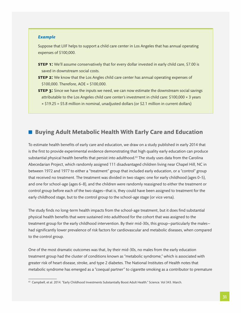
31
Example
Suppose that LIIF helps to support a child care center in Los Angeles that has annual operating
expenses of $100,000.
step 1: We’ll assume conservatively that for every dollar invested in early child care, $7.00 is
saved in downstream social costs.
step 2: We know that the Los Angles child care center has annual operating expenses of
$100,000. Therefore, AOE = $100,000.
step 3: Since we have the inputs we need, we can now estimate the downstream social savings
attributable to the Los Angeles child care center’s investment in child care: $100,000 × 3 years
× $19.25 = $5.8 million in nominal, unadjusted dollars (or $2.1 million in current dollars)
n Buying Adult Metabolic Health With Early Care and Education
To estimate health benefits of early care and education, we draw on a study published in early 2014 that
is the first to provide experimental evidence demonstrating that high quality early education can produce
substantial physical health benefits that persist into adulthood.63 The study uses data from the Carolina
Abecedarian Project, which randomly assigned 111 disadvantaged children living near Chapel Hill, NC in
between 1972 and 1977 to either a “treatment” group that included early education, or a “control” group
that received no treatment. The treatment was divided in two stages: one for early childhood (ages 0–5),
and one for school-age (ages 6–8), and the children were randomly reassigned to either the treatment or
control group before each of the two stages—that is, they could have been assigned to treatment for the
early childhood stage, but to the control group to the school-age stage (or vice versa).
The study finds no long-term health impacts from the school-age treatment, but it does find substantial
physical health benefits that were sustained into adulthood for the cohort that was assigned to the
treatment group for the early childhood intervention. By their mid-30s, this group—particularly the males—
had significantly lower prevalence of risk factors for cardiovascular and metabolic diseases, when compared
to the control group.
One of the most dramatic outcomes was that, by their mid-30s, no males from the early education
treatment group had the cluster of conditions known as “metabolic syndrome,” which is associated with
greater risk of heart disease, stroke, and type 2 diabetes. The National Institutes of Health notes that
metabolic syndrome has emerged as a “coequal partner” to cigarette smoking as a contributor to premature
63 Campbell, et al. 2014. “Early Childhood Investments Substantially Boost Adult Health.” Science. Vol 343. March.
32
coronary heart disease, and its increasing prevalence threatens to partially reverse the reduction in heart
disease risk over the past three decades that had resulted from a decline in serum low-density lipoprotein
cholesterol (“bad” cholesterol) levels. It is also one of the underlying causes of type 2 diabetes.64
By contrast, one quarter of the males in the early childhood control group was affected by metabolic
syndrome by their mid-30s. The drop in prevalence for metabolic syndrome, then, was 100 percent. Further,
the “conditional treatment effect” for metabolic syndrome among males—controlling for factors such as
cohort, the number of siblings, mother’s IQ, and high-risk index at birth—was calculated to be an even
more dramatic reduction of 189 percent when compared to the control group. The unadjusted reduction in
prevalence among females from the early education treatment group was 67 percent, and the conditional
treatment effect was 30 percent—noteworthy, but not statistically significant at the 10 percent level.65
Adults from the early childhood treatment group also experienced sustained improvements in several
other health categories, such as higher “good” cholesterol, lower prevalence of prediabetes, lower vitamin
D deficiency, lower prevalence of “severe” obesity (BMI at or above 35), and significantly lower risk of
experiencing “total” coronary heart disease. However, most of these and other conditions are either
components of a diagnosis of metabolic syndrome diagnosis or are otherwise related to the condition, and
it is difficult—even for medical professional and researchers—to disaggregate each of their contributions to
premature heart disease and type 2 diabetes. For this reason, we use metabolic syndrome as an umbrella
condition for our (conservative) estimation of early childhood education’s long-term health impacts.66
Existing research on medical costs associated with metabolic syndrome is limited. However, one study
estimates that those diagnosed with metabolic syndrome incur annual medical costs that are, on average,
about $2,000 higher than those without the syndrome ($5,732 vs. $3,581). In addition, costs increase by an
average of 24 percent per additional risk factor, and certain clusters of risk factors, or conditions, that comprise
a diagnosis of metabolic syndrome—particularly those clusters that included diabetes—are more costly.67
The research team that authored the Carolina Abecedarian Project health study did not have access to
data to adequately quantify diabetes risk, so relying on the $2,000 figure could be an underestimate of the
costs associated with observed improvements in metabolic syndrome. However, using a more conservative
figure fits our overall approach to impact assessment, so we choose to rely on it for our estimation of the
monetary value of health improvements resulting from early childhood education.
64 National Institutes of Health. 2002. hird Report of the National Cholesterol Education Program (NCEP) Expert Panel on Detection, Evaluation, and Treatment of High Blood Cholesterol in Adults (Adult Treatment Panel III). Final Report. hSeptember.65 Campbell, et al. 2014. 66 The research team tat authored the study that is the basis of our calculation plans to publish a follow-up study on the actual medical cost savings associated with long-term health impacts from the Carolina Abecedarian Project. Once these results become available to us, we will revise our impact methodology accordingly.67 Boudreau, et al. 2009. “Health Care Utilization and Costs by Metabolic Syndrome Risk Factors.” Metabolic Syndrome and Related Disorders. Vol 7, No. 4. 305-314.
33
Unfortunately, no existing research can help us determine the appropriate term of impact. If a person has
not developed metabolic syndrome by her mid-30s, it is conceivable that she could remain syndrome-free
for much longer, and it could make sense for us to assume several decades of impact. However, for the sake
of being conservative, we assume 10 years of impact starting 30 years after the start of the grant term.
Although the unadjusted and conditional reductions in metabolic syndrome prevalence for males (100
percent and 189 percent, respectively) and females (67 percent and 30 percent, respectively) were quite
different, we believe it is reasonable and conservative to assume that, if the gender breakdown in LIIF-
assisted early education facilities is approximately even—and if LIIF provides an intervention equivalent to
the Carolina Abecedarian Project, with a similar cohort of disadvantaged children—approximately 50 percent
fewer these children will have developed metabolic syndrome by their mid-30s than would be the case in
absence of this intervention (which is highly probable, as nearly all child care slots in LIIF-assisted facilities are
subsidized in some way, and as such they are a service to which families would not have typically had access).
In addition, the prevalence of metabolic syndrome among both males and females in the Carolina
Abecedarian Project control group (25 percent and 19 percent, respectively) closely approximates current
figures for the U.S. males and females over age 20 (23 percent and 22 percent, respectively) and the for
the total U.S. population over 20 (23 percent).68 As such, we believe it is reasonable to assume that, if
LIIF provides an equivalent intervention to a similar cohort of disadvantaged children, we could expect a
percentage point reduction in metabolic syndrome prevalence equivalent to 50 percent of 23 percent (11.5
percent, rounded up to 12).
However, we do not know whether the facilities that LIIF supports provide interventions that are stronger
or weaker, on average, than what the Carolina Abecedarian Project provided. On the one hand, most of the
early education programs we support do not start as early in children’s lives, nor do they last as long. On the
other hand, it is possible that programs in LIIF-supported facilities have taken advantage of four decades
worth of learning on how to run more effective early education programs, and as a result they are able to
deliver more impact over a shorter “treatment” period. Further, we are uncertain whether children in LIIF-
supported programs are more or less disadvantaged, in multiple dimensions, than those who participated in
the Carolina Abecedarian Project—let alone how variability in this regard might result in specific differences
in long-term health benefits, in comparison to the study’s findings.
68 Beltran-Sanchez, et al. 2013. “Prevalence and Trends of Metabolic Syndrome in the Adult U.S. Population, 1999–2010.” Journal of the American College of Cardiology. Vol 62, No. 8.

34
Given these uncertainties (and probably others) around applying the study’s health impacts to our portfolio
of early education, we take the admittedly rudimentary approach of assuming a linear relationship between
the age groups covered—the “term” of the intervention—and its impact. For example, if a cohort of children
attends an early education program from age 0 to 3, the hypothesized impact among this cohort would be
three-fifths of the level of impact from Carolina Abecedarian Project cohort, which covered ages 0–5. Taking
this logic a step further, we assume that each year of exposure to the “treatment” is equivalent to one-fifth
of the level of impact found in the study.
Here is how we estimate medical cost savings generated by an early education program’s impact on long-
term adult health.
step 1: Determine the number of early education (ages 0–5) slots for children from low- and moderate-
income households. On an annual basis, this is the number of children that we hypothesized will
experience the equivalent of one-fifth of a dosage of the Carolina Abecedarian Project “treatment.” Let’s
call this the number of “student-years” of exposure to the treatment of early childhood education for
each year.
step 2: Determine the contract term that these spots are required to remain affordable to children from
low- and moderate-income households.
step 3: Determine the number of children hypothesized to avoid metabolic syndrome by their mid-30s
as a result of having had access to early childhood education at this center.
• Multiply the annual number of “student-years” of exposure to the equivalent of one-fifth of the
level of treatment of the Carolina Abecedarian Project (Step 1) by the total number of years that
the program is required to remain affordable to children from low- and moderate-income families
(Step 2). This number is the total number of “student-years” of treatment equivalent to one-fifth of a
dosage of the Carolina Abecedarian Project treatment.
• Multiply this number by 0.12, signifying the assumed 50 percent reduction of the 23 percent of
children who we hypothesize would have developed metabolic syndrome as adults, were it not
for access to an early education treatment equivalent to that provided to children in the Carolina
Abecedarian Project. Then divide this number by five, signifying that we expect one-fifth the impact
for each “student-year” of exposure to the treatment.
step 4: Estimate medical cost savings generated by improved metabolic syndrome
• Multiply the number of students hypothesized to avoid metabolic syndrome as adults, as a result of
having had access to early childhood education (Step 3) by $2,000 (to signify annual medical cost
savings)
• First, estimate medical cost savings in the first year of impact (30 years after the start of the grant
term) based on some assumed increase in medical cost savings (we assume 6 percent annual
increase, as with all other health-related metrics).
• Multiply this figure by the number of children hypothesized to avoid metabolic syndrome by
adulthood (Step 3) to estimate medical cost savings M in year 1.

35
• Then, assuming 10 years of impact, and that medical costs will continue to rise during this period by
some annual rate A, estimate total medical cost savings from improvements in metabolic health using
the following formula for summing geometric sequences:
Sum = (M) – (M) × (A)10
(1 – A)
Example
Let’s imagine that LIIF supports an early education center in San Francisco with 30 slots for
children from low- and moderate-income families. The program will serve three and four year
olds, and the facility ’s contract requires that the 30 slots remain affordable to children from low-
and moderate-income families for five years.
step 1: There are 30 slots affordable to children from low- and moderate-income families.
step 2: Slots are required to remain affordable for five years.
step 3: 30 × 5 = 150 “student-years” of exposure to the treatment. 150 × .12 = 18. Then divide
by 5 ➝ 3.6 (rounded up to 4) children hypothesized to avoid metabolic syndrome by their
mid-30s as a result of having had access to early childhood education.
step 4: Assuming medical costs will rise by 6 percent per year, the $2,000 cost figure today
will be $11,487 in 30 years, translating to $45,948 in medical cost savings in the first year of
impact. Now we can estimate medical cost savings using the formula above, and estimate
that total cost savings will be $605,630.
education n Lifetime Earnings Boosts and Societal Benefits
In addition to supporting early learning and education (pre-K), LIIF helps finance the development and
expansion of charter elementary, middle, and high schools (grades K–12). There is a robust and growing
literature on the relationship of education to other social areas, such as child development, labor market
outcomes, and health—both as a contributor to outcomes in those areas (e.g., educational attainment
influences a child’s lifetime earnings potential),69 and as an outcome itself, where factors in other realms
69 See, for example: Hernandez, D. 2012. “Double jeopardy: How third-grade reading skills and poverty influence high school graduation.” Baltimore: The Annie. E. Casey Foundation. And Condit, G., and Heckman, James. 2010. “Understanding the Early Origins of the Education-Health Gradient: A Framework That Can Also Be Applied to Analyze Gene-Environment Interactions.” Perspectives on Psychological Science. Vol 5, No 5.

36
are inputs into education (e.g., educational attainment is influenced by children’s family poverty status and
exposure to early-life trauma).70
Researchers are still unpacking the complexity and potential causality around these relationships, and most
existing studies are not easily transferrable to LIIF’s approach to impact estimation because they have not
offered simple ways to leverage easy-to-collect data from schools to estimate long-term social outcomes.
Further, we do not collect data on post-secondary outcomes for students who attend LIIF-supported
schools, so we must rely on educational attainment data from grades K-12 in order to evaluate these
schools’ performance and estimate their societal impact.
However, by comparing graduation rates in the high schools we support to district averages, we can
translate Social Security Administration (SSA) projections on lifetime earnings associated with different
levels of education—in particular, graduating vs. dropping out—to estimate the incremental boost in income
generated by LIIF-supported schools.71 These projections show that today’s high school graduates will earn
nearly $1.4 million more in unadjusted, nominal dollars over the course of their lifetimes than dropouts.72
In addition, multiple estimates exist for lifetime avoided social costs to taxpayers (e.g., higher tax revenues,
lower incarceration rates, lower government medical expenditures) of graduating high school as opposed to
dropping out. The most cited study places this value at $209,000 in discounted dollars, or around $630,000
in nominal, unadjusted dollars.73
As the U.S. labor market continues to devalue the high school degree and shift towards jobs that require
some kind of higher education, graduating from high school might not sound like a proxy for success.
Absolute earnings for both dropouts and high school graduates has decreased over the past several
decades, while it has stagnated for those with four-year college degrees; the largest gains have been among
those with advanced degrees.74
On the other hand, the vast majority of students in LIIF-supported schools are from low-income families,
many living in high-poverty areas—a demographic whose children, on average, attend lower performing
schools than their middle- and higher-income peers, and for whom dropping out is a real risk with
70 See, for example: Reardon, S.F. 2011. “The widening academic achievement gap between the rich and the poor: New evidence and possible explanations.” In Duncan, G. J. and Murnane, R. J., eds. 2011. Whither opportunity? Rising inequality, schools, and children’s life chances. New York: The Russell Safe Foundation and Chicago: Spender Foundation.71 Our methodology does not control for selection bias or other potential differences in student characteristics in LIIF-supported schools compared to the rest of the district—such as the percentage of low-income or special needs students. However, the vast majority of students in LIIF-supported schools are from low-income families.72 Office of Retirement Policy, Social Security Administration. MINT 7 projections.73 LIIF tabulation of Levin, et al. 2007. See also Sum, et al. 2009. “The Consequences of Dropping Out of High School: Joblessness and Jailing for High School Dropouts and the High Cost for Taxpayers.” Northeastern University Center for Labor Market Studies.” October.74 Mitchell, Josh. 2014. “Educational Attainment and Earnings Inequality among US-Born Men: A Lifetime Perspective.” Urban Institute. April.

37
significant long-term costs, as described above.75 Further, it is reasonable to assume that at least some of
the boost in high school graduation rates generated by high-performing schools translates to increased
years of post-secondary education—even if our metrics described here do not capture this value. As such,
high school graduation rates could at least be useful proxy to indicate the extent to which the schools buck
trends and outperform alternatives in the district.76
Here is how we estimate the extent to which a LIIF-supported secondary school increases lifetime earnings
for its students.
step 1: We assume that an incremental boost in high school graduation rates translates to an average of
$1.4 million in increased lifetime earnings per student.
step 2: Determine the graduation rate of the supported charter high school.
step 3: Determine the district average high school graduation rate.
step 4: Determine the number of graduating students over the assumed term of impact (we assume
impact over the term of our financing).
step 5: With the inputs from Steps 1–4, we can estimate the monetary value of increased lifetime
earnings using this formula: (Step 2 – Step 3) × $1,400,000 × Step 4.
Here is how we estimate the extent to which a LIIF-supported secondary school generates long-term
societal savings.
step 1: We assume that over a lifetime, graduating from high school as opposed to dropping out is
associated with $630,000 in societal savings.
step 2: Determine the graduation rate of the supported charter high school.
step 3: Determine the district average high school graduation rate.
step 4: Determine the number of students over the assumed four-year term of impact.
step 5: With the inputs from Steps 1–4, we can estimate the monetary value of societal savings of
avoided dropouts or “bonus” graduates using this formula: (Step 2 – Step 3) × $630,000 × Step 4.
75 Rothwell, Jonathan. 2012. “Housing Costs, Zoning, and Access to High-Scoring Schools.” Brookings, Metropolitan Policy Program. April.76 It is also worth noting that our approach to estimating school’s “impact” is different than the one we take in some other LIIF program areas in that we do not seek to extrapolate output or program-level data (e.g., number of units) to outcomes and impact with the help of research on evidence-based practices—which, in this case, could perhaps be a certain educational philosophy to which researchers have attributed high educational attainment. Instead, we take outcomes data (e.g., high school graduation rate), however they were achieved, and use research to extrapolate to an even larger outcome/impact.

38
Example
Let’s say LIIF supports a charter high school in Oakland, California attended by 200 students. On
average, 60 percent of district students graduate from high school. In contrast, the charter high
school has a graduation rate of 90 percent.
step 1: We assume that over a lifetime, a high school graduate will earn $1,400,000 more than
a high school dropout. We also assume that graduating from high school generates lifetime
societal savings of $630,000, as compared to dropping out.
step 2: We know that the Oakland charter has a 90 percent graduate rate.
step 3: We also know that on average in Oakland, 60 percent of students graduate from high
school.
step 4: The school will attempt to graduate 200 students over the assumed four-year term of
impact.
step 5: Using the inputs from Steps 1–4, we can estimate the school’s impact on students’
nominal, unadjusted lifetime earnings ($84 million) and societal savings ($38 million).
community health centersCommunity Health Centers (CHCs) generate health system cost savings by producing better health
outcomes, delivering more efficient forms of care, and preventing costly downstream hospitalizations and
emergency room visits. The best available evidence suggests that patients who access care at CHCs generate
at least $1,000 less in annual health care expenditures relative to people who do not use CHCs, although
this figure is projected to increase with the rollout of the Affordable Care Act.77
To estimate systems-level medical cost savings generated by health centers that we support, we multiply
per-person savings by the number of unique patients served each year, and then assume impact over
the period during which we are confident the center will remain in operation—at least the term of our
financing, although centers typically operate for many years after, pending review by the Health Resources
and Services Administration. Finally, as shown below, we assume that savings will nominally increase by 6
percent each year due to rising medical costs and projected increases in savings specific to CHCs.
77 Leighton Ku, Patrick Richard, Avi Dor, Ellen Tran, Peter Shin & Sara Rosenbaum, The George Washington University School of Public Health and Health Services, Using Primary Care to Bend the Curve: Estimating the Impact of Health Center Expansion on Health Care Costs (2009), pg. 6-7.
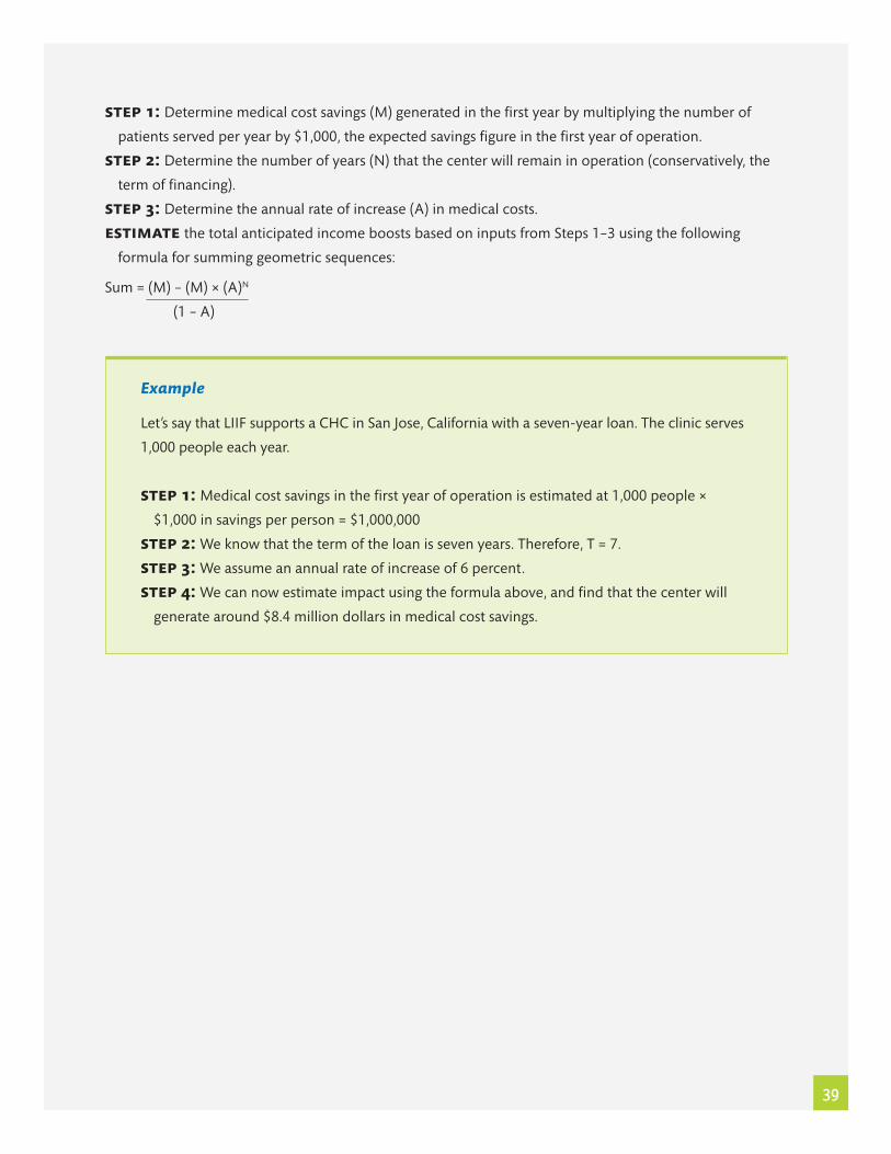
39
step 1: Determine medical cost savings (M) generated in the first year by multiplying the number of
patients served per year by $1,000, the expected savings figure in the first year of operation.
step 2: Determine the number of years (N) that the center will remain in operation (conservatively, the
term of financing).
step 3: Determine the annual rate of increase (A) in medical costs.
estimate the total anticipated income boosts based on inputs from Steps 1–3 using the following
formula for summing geometric sequences:
Sum = (M) – (M) × (A)N
(1 – A)
Example
Let’s say that LIIF supports a CHC in San Jose, California with a seven-year loan. The clinic serves
1,000 people each year.
step 1: Medical cost savings in the first year of operation is estimated at 1,000 people ×
$1,000 in savings per person = $1,000,000
step 2: We know that the term of the loan is seven years. Therefore, T = 7.
step 3: We assume an annual rate of increase of 6 percent.
step 4: We can now estimate impact using the formula above, and find that the center will
generate around $8.4 million dollars in medical cost savings.


Learn more at www.liifund.org/calculator#ImpactCalc @liifund facebook.com/liifund