University of South Florida University of South Florida

Scholar Commons Scholar Commons

Graduate Theses and Dissertations Graduate School

2011

Modeling of Solar-Powered Single-Effect Absorption Cooling Modeling of Solar-Powered Single-Effect Absorption Cooling

System and Supermarket Refrigeration/HVAC System System and Supermarket Refrigeration/HVAC System

Ammar Bahman University of South Florida, bahman.ammar@gmail.com

Follow this and additional works at: https://scholarcommons.usf.edu/etd

Part of the American Studies Commons, and the Mechanical Engineering Commons

Scholar Commons Citation Scholar Commons Citation Bahman, Ammar, "Modeling of Solar-Powered Single-Effect Absorption Cooling System and Supermarket Refrigeration/HVAC System" (2011). Graduate Theses and Dissertations. https://scholarcommons.usf.edu/etd/2993

This Thesis is brought to you for free and open access by the Graduate School at Scholar Commons. It has been accepted for inclusion in Graduate Theses and Dissertations by an authorized administrator of Scholar Commons. For more information, please contact scholarcommons@usf.edu.

Modeling of Solar-Powered Single-Effect Absorption Cooling System and

Supermarket Refrigeration/HVAC System

by

Ammar Mohammad Khalil Bahman

A thesis submitted in partial fulfillment of the requirements for the degree of

Master of Science in Mechanical Engineering Department of Mechanical Engineering

College of Engineering University of South Florida

Major Professor: Muhammad M. Rahman, Ph.D. Luis Rosario, Ph.D.

Frank Pyrtle, III, Ph.D. Craig Lusk, Ph.D.

Date of Approval: June 13, 2011

Keywords: Lithium Bromide, COP, Cooling Capacity, Simulation, Display Cases, Energy Consumption, Store Relative Humidity

Copyright © 2011, Ammar Mohammad Khalil Bahman

Dedication

To God, the Beneficent, the Merciful.

To my father, mother, brothers, and sisters,

for their great support during my graduate studies.

To my wife, Fatemah, for providing the lovely atmosphere for my study.

I dedicate this thesis especially to my beloved daughter, Laila.

Finally, to my Major Professor Muhammad Rahman,

for his immense patience and his enormous guidance.

Acknowledgements

I would like to express my sincere appreciation to Mutasim Elsheikh for his help

and support through the complete of this thesis. I would like also to thank my colleague,

Rashid Alshatti for his assistance and support during my study in the college.

Also, I would like to thank Professor Frank Pyrtle and Professor Craig Lusk for

being my committee members. I really appreciate their constant support and help.

Special thanks to Dr. Luis Rosario and Dr. Jorge C. Lallave, for their guidance

and valuable support.

i

Table of Contents

List of Tables ..................................................................................................................... iii List of Figures ......................................................................................................................v List of Symbols ................................................................................................................ viii Abstract ................................................................................................................................x Chapter 1: Introduction and Literature Review ...................................................................1

1.1 Introduction (Solar Absorption Cooling System) ..............................................1 1.2 Literature Review (Solar Absorption Cooling System) ....................................3 1.3 Introduction (Supermarket Refrigeration/HVAC System) ................................8 1.4 Literature Review (Supermarket Refrigeration/HVAC System) .......................9

Chapter 2: Solar-Powered Single-Effect Absorption Cooling System ..............................17

2.1 System Description ..........................................................................................17 2.2 Mathematical Model ........................................................................................20 2.3 Model Simulation.............................................................................................22 2.4 Results and Discussion ....................................................................................25

Chapter 3: Modeling of Supermarket Refrigeration/HVAC System for

Simple Energy Prediction ................................................................................40 3.1 Modeling and Simulation .................................................................................40 3.2 Simulation Results ...........................................................................................49 3.3 Sensitivity Analysis .........................................................................................52 3.4 Energy Consumption Analysis ........................................................................57

Chapter 4: Conclusions ......................................................................................................68 4.1 Solar-Powered Single-Effect Absorption Cooling System ..............................68 4.2 Modeling of Supermarket Refrigeration/HVAC System

for Simple Energy Prediction ...........................................................................69 4.3 Recommendations for Future Research ...........................................................70

References ..........................................................................................................................71 Appendices .........................................................................................................................76

Appendix A: MATLAB Code for Modeling of Supermarket Refrigeration/HVAC System ...........................................................................77

ii

A.1 Main M-file .....................................................................................................77 A.2 Tampa Climate Data M-file ............................................................................84 A.3 Solving for Relative Humidity M-file .............................................................89 A.4 Solving for Humidity Ratio M-file .................................................................89 A.5 Solving for Store Humidity Ratio of Old Model M-file .................................90 A.6 Solving for Store Humidity Ratio of New Model M-file................................90

About the Author ................................................................................................... End Page

iii

List of Tables

Table 2.1 Operation condition (a) [11], (b) CHEMCAD process model ................... 23 Table 2.2 Energy flow at various component of the system (a) [11], (b)

CHEMCAD process model ........................................................................ 24 Table 2.3 Comparison of COP for different refrigerants for different

cooling cycles with cooling capacity of 2.2 kW ........................................ 31 Table 3.1 Design specifications for different types of refrigerated

display case [13] ......................................................................................... 46 Table 3.2 The correlated constants c1-c6 [26] ............................................................. 46 Table 3.3 Average store relative humidity for supermarket model

simulated at 24ºC (75ºF) for each month for Tampa, Florida .................... 51 Table 3.4 Load change factors for refrigeration energy (TP) and case

defrost energy (DP) at various relative humidities and 24ºC (75ºF) ambient for multi-shelf vertical display cases [13] ......................... 59

Table 3.5 Load change factors for refrigeration energy (TP) and case

defrost energy (DP) at various relative humidities and 24ºC (75ºF) ambient for single shelf horizontal display cases [13] .................... 60

Table 3.6 Load change factor (AP) for anti-sweat energy requirements

for all types of display cases at 24ºC (75ºF) ambient [13] ......................... 60 Table 3.7 Display case refrigeration energy for simulated store at 24ºC

(75ºF) and 55% relative humidity .............................................................. 62 Table 3.8 Display case energy modifiers for various average annual

store relative humidities ............................................................................. 63 Table 3.9 Display cases annual energy requirements at various store

relative humidities ...................................................................................... 64

iv

Table 3.10 Percentage changes in energy for various store relative humidities (percent change compared to base case at 51.1% RH) ............................................................................................................. 64

Table 3.11 Changes in total store energy requirements at various relative

humidities ................................................................................................... 66

v

List of Figures

Figure 1.1 Flat-plate solar-powered single-effect absorption cooling system ...........................................................................................................2

Figure 1.2 Refrigerated display cases: (a) Vertical multi-shelf (b)

Horizontal single-shelf (c) Closed door reach-in .........................................9 Figure 2.1 Schematic diagram of the absorption cycle. ............................................... 18 Figure 2.2 Schematic diagram of the solar-powered air conditioning

system [1] ................................................................................................... 19 Figure 2.3 Hourly solar isolation for Tampa, Florida [31] .......................................... 21 Figure 2.4 Information-flow diagram for solar-powered absorption

cooling system ............................................................................................ 24 Figure 2.5 Effect of generator inlet temperature on cooling capacity and

COP ............................................................................................................ 25 Figure 2.6 Effect of generator inlet temperature on evaporator, absorber,

condenser and generator heat transfer rates................................................ 26 Figure 2.7 Effect of generator inlet temperature on generator, evaporator

and condenser temperatures ....................................................................... 28 Figure 2.8 Effect of the collector area on the heat gain using Klein,

Duffie, and Beckman equation ................................................................... 29 Figure 2.9 Comparison of cooling load and COP for CHEMCAD model

and [7] ......................................................................................................... 30 Figure 2.10 Schematic diagram of double-effect absorption cooling system ................ 32 Figure 2.11 Schematic diagram of triple-effect absorption cooling system .................. 32 Figure 2.12 Effect of generator inlet temperature on cooling capacity for

different LiBr solution concentrations ....................................................... 33

vi

Figure 2.13 Effect of generator inlet temperature on COP for different LiBr solution concentrations ...................................................................... 34

Figure 2.14 Effect of generator inlet temperature on cooling capacity for

different Phigh and Plow combinations .......................................................... 35 Figure 2.15 Effect of generator inlet temperature on COP for different

Phigh and Plow combinations ........................................................................ 36 Figure 2.16 Effect of generator inlet temperature on cooling capacity and

COP for different mass flow rates .............................................................. 37 Figure 2.17 Model hourly cooling capacity for Tampa, Florida climate ....................... 38 Figure 2.18 Model hourly coefficient of performance Tampa, Florida

climate ........................................................................................................ 39 Figure 3.1 Layout of typical supermarket .................................................................... 41 Figure 3.2 Schedule of people occupancy in supermarket model ............................... 42 Figure 3.3 Annual average hourly outdoor temperature and relative

humidity in variation Tampa, Florida (2000-2010) .................................... 43 Figure 3.4 Typical refrigerated display cases: (a) Vertical multi shelf (b)

Horizontal single shelf (c) closed door reach-in [28] ................................. 46 Figure 3.5 Information-flow diagram for store relative humidity

simulation ................................................................................................... 48 Figure 3.6 Hourly relative humidity for model store for typical year in

Tampa, Florida ........................................................................................... 50 Figure 3.7 Comparison of hourly relative humidity for [39] and

supermarket model for month of January ................................................... 53 Figure 3.8 Comparison of hourly relative humidity for [39] and

supermarket model for month of August ................................................... 53 Figure 3.9 Comparison of average monthly relative humidity for [39] and

supermarket model for Tampa, Florida ...................................................... 54 Figure 3.10 Comparison of relative humidity for experimental data [22]

and supermarket model for a typical day in Auckland, New Zealand in December 2004 ......................................................................... 55

vii

Figure 3.11 Comparison of relative humidity for experimental data [39] and supermarket model .............................................................................. 56

viii

List of Symbols

AC Collector Area [m2]

ci Correlated Constants i = 1-6 (Table 3.2)

CFD Computational fluid dynamics

COP Coefficient of performance

EER Energy efficiency ratio

FR Collector heat removal factor

h Enthalpy [kJ/kg]

HX Heat exchanger

H2O Water

LV Liquid-vapor

LLV Liquid-liquid vapor

LiBr Lithium bromide

m Mass flow rate [kg/s]

am Air curtain mass flow rate [kg/s]

NP Number of people

NRTL Non-random two-liquid

P Pressure [kPa]

q Volume flow rate [m3/s]

Q Heat transfer [kW]

ix

QL Latent heat [kW]

R Refrigerant

RH Relative humidity [%]

S Solar intensity [W/m2]

T Temperature [oC]

UL Collector overall loss coefficient [W/m2-K]

w Humidity ratio

Greek Symbols

∆ Deferential of change

Subscripts

a Ambient

abs Absorber

build Supermarket building

con Condenser

case Display case

CI Inlet of solar collector

evap Evaporator

i Process state number (i = 1, 2, 3, …etc)

infil Infiltration

shx-c Cold side of heat exchanger

shx-h Hot side of heat exchanger

space Supermarket space

S Solar

x

Abstract

This thesis consists of two different research problems. In the first one, the aim is

to model and simulate a solar-powered, single-effect, absorption refrigeration system

using a flat-plate solar collector and LiBr-H2O mixture as the working fluid. The cooling

capacity and the coefficient of performance of the system are analyzed by varying all

independent parameters, namely: evaporator pressure, condenser pressure, mass flow

rate, LiBr concentration, and inlet generator temperature. The cooling performance of the

system is compared with conventional vapor-compression systems for different

refrigerants (R-134a, R-32, and R-22). The cooling performance is also assessed for a

typical year in Tampa, Florida. Higher COP values are obtained for a lower LiBr

concentration in the solution. The effects of evaporator and condenser pressures on the

cooling capacity and cooling performance are found to be negligible. The LiBr-H2O

solution shows higher cooling performance compared to other mixtures under the same

absorption cooling cycle conditions. For typical year in Tampa, Florida, the model shows

a constant coefficient of performance of 0.94.

In the second problem, a numerical model is developed for a typical food retail

store refrigeration/HVAC system to study the effects of indoor space conditions on

supermarket energy consumption. Refrigerated display cases are normally rated at a store

environment of 24ºC (75ºF) and a relative humidity of 55%. If the store can be

maintained at lower relative humidity, significant quantities of refrigeration energy,

xi

defrost energy and anti-sweat heater energy can be saved. The numerical simulation is

performed for a typical day in a standard store for each month of the year using the

climate data for Tampa, Florida. This results in a 24 hour variation in the store relative

humidity. Using these calculated hourly values of relative humidity for a typical 24 hour

day, the store relative humidity distribution is calculated for a full year. The annual

average supermarket relative humidity is found to be 51.1%. It is shown that for a 5%

reduction in store relative humidity that the display case refrigeration load is reduced by

9.25%, and that results in total store energy load reduction of 4.84%. The results show

good agreement with available experimental data.

1

Chapter 1: Introduction and Literature Review

1.1 Introduction (Solar Absorption Cooling System)

The energy needed to process and circulate air in buildings and rooms to control

humidity, temperature, and cleanliness has increased significantly during the last decade

especially in developing countries. This energy demand has been caused by the

increment of thermal loads to fulfill occupant comfort demands, climate changes, and

architectural trends. The growth of electricity demand has increased especially at peak

loads hours due to high use of driven vapor compression refrigeration machines for air

conditioning. In addition, the consumption of fossil fuels and the emissions of greenhouse

gases associated with electricity generation lead to considerable environmental

consequences and monetary costs. Conventional energy resources will not be enough to

meet the continuously increasing demand in the future. In this case, an alternative

solution for this increasing demand of electrical power is solar radiation, available in

most areas and representing an excellent supply of thermal energy from renewable energy

resource.

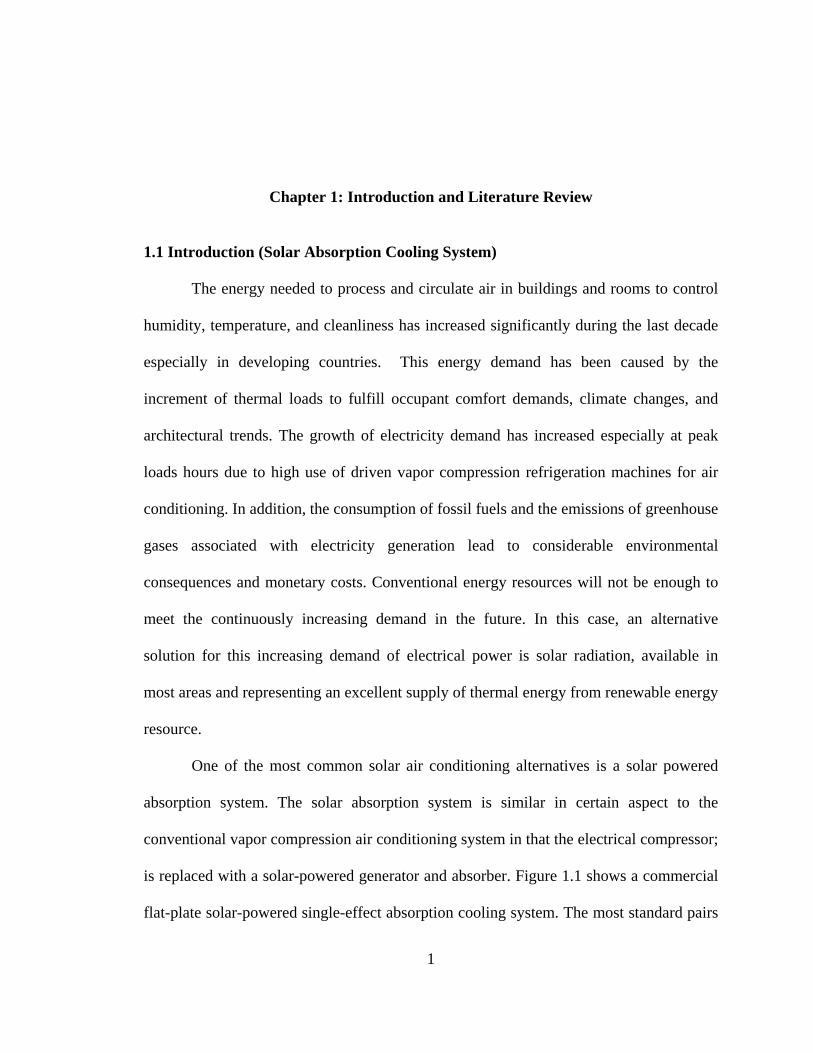
One of the most common solar air conditioning alternatives is a solar powered

absorption system. The solar absorption system is similar in certain aspect to the

conventional vapor compression air conditioning system in that the electrical compressor;

is replaced with a solar-powered generator and absorber. Figure 1.1 shows a commercial

flat-plate solar-powered single-effect absorption cooling system. The most standard pairs

2

of chemical fluids used include lithium bromide-water solution (LiBr-H2O), where water

vapor is the refrigerant and lithium bromide is the absorbent, and ammonia-water

solution (NH3-H2O) with ammonia as the refrigerant and water the absorbent [1]. The

implementation of computer modeling of thermal systems offer a series of advantages by

eliminating the cost of building prototypes, the optimization of the system components,

estimation of thermal energy loads delivered or received from or into the system, and

prediction of variations of the system parameters (e.g. temperature, pressure, mass flow

rate).

Figure 1.1: Flat-plate solar-powered single-effect absorption cooling system.

Chiller

Solar collector

3

1.2 Literature Review (Solar Absorption Cooling System)

A number of experimental and theoretical studies of solar-powered air-

conditioning systems have been done in the past. Wilbur and Mitchell [2] compared

theoretically single-stage, lithium bromide-water absorption cooling system heated from

flat-plate solar collector to an ammonia-water system, and the lithium bromide system

was preferred. It was shown that it required smaller cooling towers than the conventional

one.

Li and Sumathy [3-4] experimentally studied a solar-powered absorption air

conditioning system of lithium bromide-water solution as the refrigerant fluid. Their

experimental results showed that using a partitioned hot-water storage tank is necessary

to enhance the reliability of the system and achieve a continuous process operation.

Florides et al. [5] numerically studied a solar absorption cooling system with

TRNSYS simulation program for the weather conditions of Nicosia, Cyprus. A system

optimization was carried out in order to select the appropriate type of collector, the

optimum size of the storage tank, collector slope and area under the two most favorable

thermostats setting of the auxiliary boiler. The final optimized system consisted of a 15

m2 compound parabolic solar collector tilted by 30o from the horizontal and a 0.6m3 hot-

water storage tank.

Atmaca and Yigit [6] developed a modular computer program for a solar-powered

single-stage absorption cooling system using the lithium bromide-water solution as their

working refrigerant. They examined various cycle configurations and solar energy

parameters at Antalya, Turkey. The effects of hot water inlet temperatures on the

coefficient of performance (COP) and the surface area of the absorption cooling

4

components were studied. The minimum allowable hot water inlet temperatures or

reference temperature effects on the coefficient of performance were examined as part of

their research. Their results showed that the increment of reference temperature decreases

the absorber and solution heat exchanger surface area, and increases the system COP,

while the size of the other components remains unchanged. Atmaca and Yigit [6] showed

that evacuated, selective surface solar collector is the best option for the effective

operation of their solar-power absorption cooling system. Their results showed that solar-

power absorption cooling system requires a high performance collector.

Florides et al. [7] presented a method to evaluate the characteristics and

performance of a single stage LiBr-water absorption machine. The heat and mass transfer

equations including the appropriate equations of the working fluid properties were

employed in a computer program as part of their research. The sensitivity analysis results

showed that the greater difference between inlet and outlet concentrations of the LiBr-

water solution at the absorber will reduce the mass flow rate. Florides et al. determined

the cost for a domestic size absorber cooler, and concluded that despite the high price of

the LiBr–water absorption cooling system in comparison with a electrical chiller of

similar capacity, the absorption system remained favorable due to the use of renewable

energy sources and waste heat, whereas the electric chiller uses electrical power that is

produced from fossil fuels and has harmful effects on the environment. Assilzadeh et al.

[8] studied a solar absorption cooling system that has been designed for Malaysia climate

and similar tropical regions using TRNSYS numerical simulations. They used evacuated-

tube solar collector for energy input to the absorption cooling system and Lithium

bromide-water mixture as the working fluid. They proved that evacuated tube solar

5

collector provides high cooling performance at high temperature due to its high efficiency

under this weather condition. The results showed that the cooling capacity of the system

is large during periods of high solar radiation energy. The authors suggested a 0.8 m3 hot-

water storage tank in order to increase the reliability of the system and to achieve

continuous operation for a 3.5 kW (1 refrigeration ton) system consists of 35 m2

evacuated tubes solar collector sloped by 20o as an optimum system at Malaysia’s

weather condition.

Mittal et al. [9] performed numerical simulations of a solar-powered single-stage

absorption cooling system using a flat-plate solar collector and LiBr-water solution. A

modular computer program was developed for the absorption system to simulate various

cycle configurations with the help of weather data of Bahal village, district of Bhiwani on

the western fringe of Haryana, India. The authors studied the effects of hot-water inlet

temperatures on the coefficient of performance and the surface area of the absorption

cooling component. Their results showed that the increment of the hot-water inlet

temperature decreases the absorber and solution heat exchanger surface area, while the

sizes of the other components remain the same. The authors examined the effect of

reference temperature, the minimum allowable hot-water inlet temperature on the fraction

of total load met by non-purchased energy (FNP), and the coefficient of performance.

They concluded that high reference temperature increases the system COP and decreases

the surface area of the system components; however, lower reference temperature shows

better results for FNP. Sayegh [10] investigated an absorption cooling system powered

with solar energy with the use of a thermal storage tank, auxiliary heater and flat plate

solar collector for the weather conditions of Aleppo, Syria. Lithium bromide-water is

6

used as a working fluid for the system. A computational program is prepared to

investigate the effect of varying the generator temperature between 80 to 100oC, and the

evaporator temperature between 5-15oC on the coefficient of performance (COP) and

solar useful heat gain of the absorption cooling system. Their results show that higher

COP values are obtained by the increment of the generator temperature and the

temperature drop of the evaporator. In addition, Sayegh [10] recommend the installation

of seasonal thermal storage tank to decrease the AC load differences, which must be

supplied by an auxiliary heater.

Balghouthi et al. [11] assessed the feasibility of solar-powered absorption cooling

system under Tunisian weather conditions. They used TRNSYS and EES software’s

including a meteorological year data file containing the climatic condition of Tunis, the

capital of Tunisia, in order to select and size the different components of the solar system

to be installed. Their system was optimized for a typical building of 150m2 and water

lithium bromide absorption chiller with a capacity of 11 kW, and 30m2 flat plate solar

collector area tilted by 35o from the horizontal and a 0.8m3 hot-water storage tank. The

simulation results showed that solar-power absorption cooling system is suitable under

Tunisian conditions. The potential of integrated solar absorption cooling and heating

systems for building applications were evaluated by Mateus and Oliveira [12]. The

authors used TRNSYS software as a basis for their assessment. Different building types

such as: residential, office and hotel and three different locations and climates from

Berlin (Germany), Lisbon (Portugal), and Rome (Italy) were considered as part of their

assessment. They ran the model for a whole year (365 days), according to control rules

whether heating or cooling, and with the possibility of combining cooling, heating and

7

domestic hot water (DHW) applications. The different local costs for energy i.e. gas,

electricity and water were taken into account for all cases. The authors concluded that

residential house and hotel building types are the cases where the solar integrated system

has a higher economic feasibility. For current energy costs, Rome was the only city to

achieve a break-even situation. Their results showed a reduction in solar collector area

between 15 to 50% by using vacuum tube collectors instead of flat-plate collectors.

Conversely, flat-plate collectors lead to higher economic viability compared to vacuum

tube collectors. To increase their marketability, integrated solar absorption cooling and

heating systems need to reduce the initial costs of absorption chiller and solar collectors,

considering the current costs of energy sources i.e gas and electricity. An optimization of

solar collector size and other system parameters and CO2 emissions savings were also

assessed. An excellent reduction of CO2 emissions were obtained by using an integrated

solar system for combined heating and cooling in comparison with conventional systems.

However, only a small number of papers could be found that considered a solar-powered

cooling system using a flat-plate solar collector and LiBr-H2O mixture as the working

fluid.

The present study attempts to carry out a comprehensive investigation of a solar-

powered single-effect absorption cooling system by using a flat-plate solar collector and

LiBr-H2O mixture as a working fluid. The modeling of the system components is carried

out with the CHEMCAD software. Numerical computations were used to study the effect

of inlet generator temperature on the cooling capacity and cooling performance of the

system by varying different parameters (i.e. evaporator pressure, condenser pressure,

mass flow rate, and LiBr-water solution concentration). The main contribution is to carry

8

out the cooling performance of solar-powered absorption cooling system by the

comparison with a conventional vapor-compression system for different refrigerants. In

addition, the cooling performance is also assessed for a typical year in Tampa, Florida.

1.3 Introduction (Supermarket Refrigeration/HVAC System)

Nowadays, the supermarket is a high-volume food sales outlet with maximum

storage turnover. Most food products need to be kept under certain ambient temperature

and relative humidity during operation hours. These foods are displayed in highly

particular and flexible refrigerated display cabinets as shown in Figure 1.2. Most of the

retail food can be spoiled unless refrigerated. These foods include meat, dairy products,

frozen food, ice-cream and frozen desserts, and different individual items such as bakery

and deli products and cooked meals. When a refrigerated display case operates in the

supermarket environment, it exchanges heat and moisture within its environment. The

moisture exchange between the display case and the store environment is the most

troublesome part of this event due to an increase in energy requirement to maintain a

satisfactory temperature within the display case. Nevertheless, maintaining a low relative

humidity in the store environment requires an air-conditioning system with satisfactory

performance characteristics. This maybe quite expensive with high operating cost. On the

other hand, the operating cost of the display cases will be lower due to less latent load on

the refrigeration coil, fewer defrosts to be required and less anti-sweat heater operation.

Higher store relative humidity will result in lower operating cost of the air- conditioning

equipment resulting in higher condensation on the display case walls, products and

further frost on the evaporator coils.

9

(a) (b)

(c)

Figure 1.2: Refrigerated display cases: (a) Vertical multi-shelf (b) Horizontal single-shelf (c) Closed door reach-in.

1.4 Literature Review (Supermarket Refrigeration/HVAC System)

In the literature, a reasonable number of research studies on refrigerated display

cases have been reported. Howell and Adams [13] studied the effects of indoor space

conditions on refrigerated display case performance. Howell [14, 15] developed a

procedure that evaluates the effects of relative humidity on the energy performance of

refrigerated display case energy requirement, anti-sweat heater energy, and defrost

energy requirements. Howell [14] show that the savings in energy of the display cases

ranged from 5% for closed door reach-ins cases to 29% for multi-shelf display cases

when operated at store relative humidity of 35% rather than at 55%. The majority of the

10

cases saved 20% to 30% of their compressor energy, 40% to 60% in defrost energy, and

19% to 73% in anti-sweat heater operation for different types of display cases. The

increment of AC energy requirement when the store operated at 35% relative humidity

rather than 55%, ranged from 4% to 8% depending on the energy efficiency ratio (EER)

value of the air-conditioning unit.

Tassou and Datta [16] investigated the effects of in-store environmental

conditions on frost accumulation at the evaporator coils of open multi-deck refrigerated

display cabinets. Their field and environmental chamber-based tests have shown that

ambient relative humidity and temperature of a store have a significant effect on the rate

of frost formation on the evaporator coils, with the effect of relative humidity being more

evident than the effect of temperature. They concluded that a considerable opportunity

exists to implement sophisticated defrost control strategies to save energy and improve

temperature control. Orphelin et al. [17] discussed a new approach to estimate impacts of

temperature and humidity set points on the total energy balance of typical French

supermarkets. Their model took into account the cold aisle effect and the occurrence of

thermal coupling between the supermarket display cases and the air-conditioning system.

Their results showed that it is not cost effective to maintain a lower relative humidity

level under 40% within the store during summer time. In addition, their results showed

that the performance of air-conditioning and refrigeration systems of the operating the

display cases, have to be well known in order to define an acceptable set point in terms of

energy consumption and customer comfort.

Rosario and Howell [18] experimentally evaluated the energy savings produced

by reducing the relative humidity of the store. Eight supermarkets in the Tampa, Florida

11

area were monitored for twelve hours and seven day periods between November 1997

and October 1998 in order to know the typical store relative humidity prior to its potential

reduction. Five different areas of the eight supermarkets were monitored. The relative

humidity within the store differed up to 20% and the average annual relative humidity

between different stores varied up to 12%. Their results show that the average relative

humidity of all stores have a minimum value of 37% during the month of March and a

maximum value of 56% during the month of September. The annual average value for all

stores is 45%. An algebraic expression based on experimental results was used to

correlate indoor humidity ratio as a function of outdoor humidity ratio. Their results

showed that the theoretical moisture balance model’s prediction was within ±10% in

comparison with the experimental data. They concluded that the total store energy bill

(i.e. display cases, air-conditioning and lights) could be reduced up to 5% by lowering the

store relative humidity by 5%. The store relative humidity reduction of 1% represented

the savings of 18,000 to 20,000 kWh annually.

Kosar and Dumitrescu [19] provided an updated review of currently available

databases that address the effect of supermarket humidity on refrigerated case energy

performance from computer simulations, laboratory tests, and field evaluations. Their

database reviewed findings and tabulated those by case type, humidity range, and energy

performance impact which were separated by compressor energy, defrost energy, and

anti-sweat energy. Their findings revealed that the reduction in anti-sweat energy heater

operation, compressor energy reductions, and electrical defrost reductions represent the

55%, 44%, and 1% of the store energy savings potential respectively. Although these

conclusions differ with the store mix of case types and controls for anti-sweat and defrost

12

operation, it is clear that anti-sweat heater requirements deserve as much attention as

compressor or refrigeration loads of display cases at low humidity levels.

Chen and Yuan [20] experimentally invistegated the effects of some important

factors on performance of a multi-shelf refrigerated display case. The factors include the

ambient temperature and humidity, discharge air velocity, night covers and air flow from

perforated back panels. Both inside and temperature distribution and cooling were

studied. The results showed that ambient temperature and relative humidity increse

causing the temperature and heat gain of the display case to increase. In addition, the

results were in great significance to the optimum design of display cases and energy

management of supermarkets.

Due to the importance of numerical modelling to have effective and effiecient

refrigerated systems, Smale et al. [21] reviewed all numerical modelling techniques and

the application of CFD during the period of 1974 to 2005 for the prediction of airflow in

refrigerated food applications including cool stores, transport equipments, and retail

display cabinets.

Getsu and Bansal [22] numerically and experimentally analysed evaporator in

frozen food display cases at low temperature in the supermarket in Auckland, New

Zealand. Extensive experiments were conducted to measure store and display case

relative humidities and temperatures, and pressures, temperatures and mass flow rates of

refrigerants. The mathematical model used different empirical correlations of heat

transfer coefficient and frost properties for the heat exchanger in order to investigate the

influence of indoor conditions on the performance of the display cases. Experimental data

were used to validate the model so that the model would be a tool for designers to

13

evaluate the performance of supermarket display case heat exchangers under different

retail store conditions.

Ge et al. [23] integrated CFD with cooling coil model to simulate and analyse the

performance of multi-deck medium temperature display case. The 2D CFD model can

predict the air dynamics of air flow, heat and mass transfer among the air flow, food

products and ambient space air. The model simulated different pipe and fin structures and

circuit arrangements, with the outputs from the cooling coil model used as the inputs to

the CFD model and vice versa. A typical multi-deck medium temperature display case

was selected as a prototype and mounted into an air conditioned chamber to validate this

integrated model. The validated model was used to examine the cabinet performance and

explore the optimal control strategies at various operating conditions and design

conditions.

The importance of an air curtain in refrigerated display cases modeling motivated

many researches and a number of studies have been published on the development of an

air curtain. Howell et al. [24] theoretically and experimentally investigated the heat and

moisture transfer through turbulent plane air curtains. They investigated the performance

of air curtain by the variation of the number of jets, thickness, width, height, velocity,

turbulence level of the air curtain, and pressure and temperature difference across the air

curtain. An eddy viscosity model was used with finite difference technique to calculate

the sensible, latent, and total heat transfer through air curtains. Their results showed that

the total heat transfer is directly proportional to the initial velocity and the temperature

difference across the air curtain, including the significant effect of the initial turbulence

14

intensity that could reach up to 32% increment of heat and moisture transfer through an

air curtain.

Howell and Shibata [25] experimentally investigated the relationship between the

heat transfer through a recirculated air curtain and its deflection modulus. The deflection

modulus was defined as the ratio of the initial momentum of the air curtain jet and the

transverse forces magnitude in which the air curtain attempts to seal against. Their

research investigated the performance of air curtain by the variation of the number of jets,

thickness, width, height, velocity, turbulence level of the air curtain, and pressure and

temperature difference across the door opening. The authors demonstrated that there is an

optimum flow velocity for the air curtain to seal the doorway and minimize the heat

transfer rate and moisture effect. Their findings show that transverse and longitudinal

temperature differences can be used as one of the correlating parameters of recirculated

air curtains, including the value of the deflection modulus which exists for each air

curtain configuration which minimizes the heat transfer rate across the air curtain.

Ge and Tassou [26] developed a comprehensive model, based on the finite

difference technique, which can be used to predict and optimize the performance of air

curtains. Based on the results obtained from their model, correlations for the heat transfer

across refrigerated display case air curtains have been developed to enable quick

calculations and parametric analyses for design and refrigeration equipment sizing

purposes. In this study, the authors have shown that both the finite difference and

simplified models can be used to determine the total cooling load of vertical refrigerated

display cases with a reasonable degree of accuracy.

15

Cui and Wang [27] used a computational fluid dynamics (CFD) method to

evaluate the energy performance of an air curtain for horizontal refrigerated display cases

and optimize their design. The CFD method was validated by comparing the CFD

calculations with experimental results. The authors studied the key factors that influence

the air curtain cooling load such as: air curtain velocity, the height and shape of products

inside the display case, temperature difference between the inlet and ambient air, and the

relative humidity of the ambient. Their results showed that there is an optimum value for

the inlet velocity of the air curtain, while other design parameters remain unchanged.

They also found that the air curtain is heavily affected by both the inlet air temperature

and the relative humidity of ambient air. The larger the temperature difference and/or

relative humidity difference between the inlet and ambient air, the more intensive will be

the heat and mass transfer between the air curtain and the ambient air. Therefore,

properly controlled indoor conditions, i.e. dry-bulb temperature and relative humidity,

could well balance the cooling load of the store against that of the display cases and help

achieve overall energy efficiency. Cui and Wang [27] concluded that the CFD method is

an effective and feasible tool for the optimal design and performance evaluation of air

curtain of horizontal refrigerated display cases.

Navaz et al. [28] presented a comprehensive discussion on past, present, and

future research focused on display case air curtain performance characterization and

optimization. Ge and Cropper [29] developed a display case model by the integrating

three main component sub-models, an air-cooling finned-tube evaporator, an air curtain

and a display case body at steady state. In their work, they described the analysis and

performance comparison of a display cabinet system using R404A and R22 as the

16

refrigerants. They concluded that the total cooling load of display case and refrigerant

mass flow rate increased at higher ambient air humidity. In addition, the increment of

ambient air humidity will affect significantly the latent cooling load more than its

sensible load. The increment of cooling load or refrigerant mass flow rate of the R404A

refrigerant increased the power consumption of the refrigeration unit. At a specified

operating condition, R404A refrigerant display case required greater cooling loads and

refrigerant mass flow rates than R22 refrigerant units.

The objective of this work is to model a supermarket refrigeration/HVAC system,

and to develop a numerical simulation for this model using MATLAB. The model is

integrating the air curtain model developed by [26] for display cases within the main

supermarket model. The simulation is performed for a typical day under standard store

conditions for each month of the year using climate data for Tampa, Florida. A

parametric study of this system and a prediction of energy consumption are done to study

the effect of indoor space conditions on supermarket energy consumption. A sensitivity

analysis is performed for the proposed model and validated with available experimental

data. The main contributions are to validate the air curtain model developed by [26]

within the supermarket model for Tampa, Florida weather conditions and calculate the

energy consumption when the store relative humidity is reduced.

17

Chapter 2: Solar-Powered Single-Effect Absorption Cooling System

2.1 System Description

The solar-powered absorption cycle consists of four major parts, i.e., a generator,

a condenser, an evaporator and an absorber. These major components are divided into

three parts by one heat exchanger, two expansion valves and a pump. Schematic

diagrams of the solar-powered cooling system are shown in Figures 2.1 and 2.2. Initially,

the collector receives energy from sunlight and heat is accumulated in the storage tank.

Subsequently, the energy is transferred through the high temperature energy storage tank

to the refrigeration system. The solar collector heat is used to separate the water vapor,

stream number 2, from the lithium bromide solution, stream number 3, in the generator at

high temperature and pressure resulting in higher lithium bromide solution concentration.

Then, the water vapor passes to the condenser where heat is removed and the vapor cools

down to form a liquid, stream number 4. The liquid water at high pressure, stream

number 4, is passed through the expansion valve, stream number 9, to the evaporator,

where it gets evaporated at low pressure, thereby providing cooling to the space to be

cooled. Subsequently, the water vapor, stream number 5, goes from the evaporator to the

absorber. Meanwhile, the strong lithium bromide solution, stream number 3, leaving the

generator for the absorber passes through a heat exchanger in order to preheat the weak

solution entering the generator, and then expanded to the absorber, stream number 6. In

the absorber, the strong lithium bromide solution absorbs the water vapor leaving the

18

evaporator to form a weak solution, stream number 7. The weak solution, stream number

8, is then pumped into the generator and the process is repeated.

6

9

4

5

Pump

Condenser

Ev aporator

Exp v alv e

Exp v alv e

Absorber

Generator

10

HE

7

2

31

8

Solar collector

Cooling tower

Water v apor

LiBr

Figure 2.1: Schematic diagram of the absorption cycle.

19

Figure 2.2: Schematic diagram of the solar-powered air conditioning system [1].

Generally, the heat is removed from the system by a cooling tower. The cooling

water passes through the absorber first then the condenser. The temperature of the

absorber has a higher influence on the system efficiency than the condensing temperature

of the cooling tower where the heat is dissipated to the environment. In the case that the

sun is not shining, an auxiliary heat source is used by electricity or conventional boiler to

heat the water to the required generator temperature. It is highly recommended to use a

partitioned hot-water storage tank to serve as two separate tanks. In the morning, the

collector system is connected to the upper part of the tank, whereas in the afternoon, the

whole tank would be used to provide heat energy to the system.

20

2.2 Mathematical Model

A control volume is taken across each component i.e. the generator, absorber,

evaporator, condenser and heat exchanger to analyze the working conditions of all

components of the system. The mass and the energy balances are performed and a

computer simulation is developed for the cycle analysis. A control volume analysis

around each component, which covered the rate of heat addition in the generator, and the

energy input of the cycle, is given by the following equation:

Qgen = h2m2 + h3m3 − h1m1 (1)

The rate of heat rejection out of the condenser is given by the following equation:

)( 422 hhmQcon −= (2)

The rate of heat absorption of the evaporator is given by the following equation:

)( 952 hhmQevap −= (3)

The rate of heat rejection of the absorber is given by the following equation:

173625 mhmhmhQabs −+= (4)

An energy balance on the hot side of the heat exchanger is given by the following

equation:

)( 1033 hhmQ hshx −=− (5)

Similarly an energy balance on the cold side of the heat exchanger is given by the

following equation:

)( 811 hhmQ cshx −=− (6)

The overall energy balance on the heat exchanger is satisfied if cshxhshx QQ −− = which is

valid in this case.

21

Coefficient of performance (COP) according to Figure 2.1 is defined as follows:

gen

evap

QQ

COP = (7)

The solar collector was modeled in the manner proposed by Klein, Duffie, and

Beckman [30]. The basic equation for flat-plate solar collector is given by:

QS = FR AC [S −UL (TCI − Ta )] (8)

For simplicity, the collector heat removal factor of FR = 0.8 is used. Average solar

intensity is shown in Figure 2.3 for typical year in Tampa, Florida [31]. The average flat-

plate solar collector loss coefficient of UL = 3.0 W/m2-K is held constant. The collector

inlet temperature TCI, and the ambient temperature Ta are assumed to be 80oC and 30oC,

respectively.

Figure 2.3: Hourly solar isolation for Tampa, Florida [31].

22

2.3 Model Simulation

CHEMCAD [32] was used to simulate the solar-powered lithium bromide

absorption system. The generator and absorber were modeled by using a multipurpose

flash column. CHEMCAD uses the flash column to visualize generator and absorber

operations. Simultaneously, a modular mode was used to solve the algebraic equations of

the flow sheet. The Non-random two-liquid (NRTL) model and latent-heat enthalpy

model were used in the simulation to obtain the thermodynamic properties and phase

equilibrium of the Lithium bromide solution. The NRTL model software keeps all flashes

as three-phase flashes (LLV) or two-phase flashes (LV). Liquid phase activity

coefficients are calculated by the NRTL equation by the known values of the liquid phase

mass fraction. The NRTL equation is a good method to solve the binary mixture where

equilibrium prevails between liquid and vapor [33]. Previous studies have shown that the

NRTL equation is in good agreement with the experimental phase equilibrium of Lithium

bromide solution [34]. The simulation model was also compared with a solar absorption

air conditioning study which was carried out in Tunisia using TRNSYS and EES

programs [11]. The following parameters and assumptions were used in the simulation:

Strong solution concentration of 0.561 (LiBr mass fraction);

Strong solution mass flow rate m1 = 0.056 kg/s;

The water vapor mass flow rate m2 = 0.0048 kg/s;

The high and low pressures of the system were set at 6.601 and 0.9 kPa, respectively;

Generator heat duty Qgen = 15.26 kW;

Pressure drops were neglected;

Work input by the pump was neglected.

23

The comparison of present numerical results and Balghouthi et al. [11] results are shown

in Table 1 and 2. The numerical data obtained are in good agreement with Balghouthi et

al. [11] results.

Table 2.1: Operation condition (a) [11], (b) CHEMCAD process model.

Stream T (oC) P (kPa) x (kg LiBr/kg solution)

m (kg/s)

(a) (b) (a) (b) (a) (b) (a) (b) 1. Pump outlet 36.2 36.2 6.601 6.601 0.561 0.561 0.056 0.056 2. Condenser inlet 70 71.2 6.601 6.601 0 0 0.0048 0.0048 3. Generator outlet 84.6 71.2 6.601 6.601 0.613 0.614 0.0512 0.0512 4. Condenser outlet to

exp. valve 38 37.8 6.601 6.601 0 0 0.0048 0.0048

5. Vapor from evaporator to absorber

4.4 5.4 0.9 0.9 0 0 0.0048 0.0048

6. Solution inlet in absorber

47.1 31.3 0.9 0.9 0.613 0.614 0.0512 0.0512

7. Absorber outlet 36.2 36.2 0.9 0.9 0.561 0.561 0.056 0.056 8. Generator inlet

from heat exchanger

62.4 62.4 6.601 6.601 0.556 0.561 0.056 0.056

9. Evaporator inlet from expansion valve

5.5 5.4 0.9 0.9 0 0 0.0048 0.0048

10. Absorber inlet from heat exchanger

53.6 69.3 6.601 6.601 0.613 0.614 0.0512 0.0512

11. Generator inlet from heat exchanger

62.4 62.4 6.601 6.601 0.556 0.561 0.056 0.056

24

Table 2.2: Energy flow at various component of the system (a) [11], (b) CHEMCAD process model.

Description Symbol Energy (kW) (a) (b)

Evaporator Qevap 11.31 11.26 Absorber Qabs 14.67 14.61 Generator Qgen 15.26 15.26 Condenser Qcon 11.89 11.90 Coefficient of performance COP 0.74 0.74

The input data required for simulating the system consists of the following:

generator temperature, absorber temperature, generator and condenser pressure,

evaporator and absorber pressure, pump output pressure, mass flow rate entering

generator, lithium bromide solution concentration entering the generator and fixed

saturated liquid state from heat exchanger to generator. Figure 2.4 shows flow-diagram

for how simulation works using input data. The output includes the generator heat gain,

cooling capacity and COP.

Figure 2.4: Information-flow diagram for solar-powered absorption cooling system.

h8

m1, h7 h6

h5

h10

Back to Generator

h4

h3 m3, h3

m2, h2 Condenser

Absorber Evaporator

Pump

HX Exp. Valve

Exp. Valve

m1, %LiBr

P1, T1 Generator

25

2.4 Results and Discussion

Simulation results are presented here for the performance of the solar-powered

absorption cooling system. The effect of the variation of the inlet generator heating water

temperature is shown in figure 2.5. The cooling capacity varies approximately linearly

starting from a low value of 0.47 kW up to 16 kW. The COP rises from a low value of

0.82 to reach a constant value of 0.94. The cooling capacity increases as the inlet

generator temperature increases. The COP of the system increases slightly when the heat

source temperature increases.

Figure 2.5: Effect of generator inlet temperature on cooling capacity and COP.

The COP would be expected to increase significantly with increasing

generator/source temperature, but as the generator/source temperature increases, the heat

transfer in all the heat exchangers of the system also increases as shown in Figure 2.6.

26

The figure shows linear increase in the heat transfer in all of evaporator, condenser and

absorber when varying the inlet generator temperature.

Figure 2.6: Effect of generator inlet temperature on evaporator, absorber, condenser and

generator heat transfer rates.

Figure 2.7 shows that the evaporator temperature decreases with the source

temperature while the generator outlet solution temperature and the condensation

temperature increase. The generator inlet temperature could not be increased or decreased

too much because of the crystallization of the lithium bromide. Because lithium bromide

is a salt, in its solid state it has a crystalline structure. There is a specific minimum

solution temperature for any given salt concentration when lithium bromide is dissolved

in water. The salt begins to leave the solution and crystallize below this minimum

temperature. In an absorption system, if the LiBr-solution concentration is too high or if

27

the LiBr-solution temperature is reduced too low, crystallization may occur [7]. The

crystallization influences the cycle performance and the temperatures at different streams.

There are several causes for crystallization. Air leakage into the system is one of most

common reason for crystallization. Air leakage results in increased pressure in the

evaporator. This, in turn, results in higher evaporator temperatures and, consequently,

lower cooling capacities. In the other case, at high load conditions, the control system

increases the heat input to the generator, resulting in increased solution concentrations to

the level where crystallization may occur. Non-absorbable gases, like hydrogen,

produced during corrosion, can also be present, this can reduce the performance of both

the condenser and the absorber. Electric power failure is found to be another reason for

crystallization [7]. Crystallization is most likely to occur when the machine is stopped

while operating at full load, when highly concentrated solutions are present in the

solution heat exchanger. To solve this problem, during normal shutdown, the system

should go into a dilution cycle, which lowers the concentration of the LiBr-solution

throughout the system, so that the machine may cool to ambient temperature without

crystallization occurring in the solutions.

28

Figure 2.7: Effect of generator inlet temperature on generator, evaporator and condenser

temperatures.

Figure 2.8 shows the generator heat gain when increasing the collector area using

Klein, Duffie and Beckman equation [30]. The greater the collector area the greater the

heat gained. This can be good for the auxiliary boiler. Once the heat gained is increased,

less heat is required from the auxiliary boiler to maintain the required generator

temperature.

29

Figure 2.8: Effect of the collector area on the heat gain using Klein, Duffie, and Beckman

equation.

Figure 2.9 illustrates comparison of cooling load and coefficient of performance

for both CHEMCAD model and TRNSYS model [11]. The current model shows

matching trends with the previous study of [11]. Increasing the heat source temperature

increases the cooling capacities linearly for both models. The COP for both models has

the same trend. For temperatures less than 70oC, the COP increases slightly. As the

generator inlet temperature increases, the COP reaches constant values of 0.75 and 0.72

for both CHEMCAD and TRNSYS models, respectively. The reason for this discrepancy

is due to different equations of state used in the softwares; NRTL was used in

CHEMCAD and nonlinear equation solver was used in TRNSYS. Also, for simplicity,

the overall heat transfer coefficients for all major components are assumed to be

negligible in the current model, this, in turn, results in higher cooling load and lower heat

in the generator and so on higher COP.

30

Figure 2.9: Comparison of cooling load and COP for CHEMCAD model and [11].

The change of the cooling performance (COP) of refrigerants for different cooling

cycles is reported in Table 2.3. Özkan et al. [35] compared the performance of different

refrigerants like R-600a, R-134a, R-290, R-1270, R-32, R-22, and R-152a in vapor

compression refrigeration cycle. He et al. [36] examined the efficiency characteristics of

R-22+DMF, R-134a+DMF and R-32+DMF in solar-powered absorption cooling system.

Table 2.3 compares the COP for [35] and [36] with the current study. A cooling load of

2.2 kW was used as a reference to compare between the refrigerants. According to the

table, the COP of R-22 is the highest while the COP of R-32+DMF is the lowest.

Refrigerants R-134a, R-32 and R-22 have COP values larger than one. In the other hand,

the mixtures Libr-H2O, R-22+DMF, R-134a+DMF and R-32+DMF have COP values

less than one. Both the refrigerant and refrigeration cycle influence the value of COP. It

is well known that the vapor compression refrigeration cycles have COP value larger than

31

one, while the solar-powered absorption systems have COP value less than one [37]. This

is due to the different definition for the COP for the vapor compression system and the

absorption system. If the COP definition of vapor compression cycle was used to find the

COP of the solar absorption cycle, the COP of the solar absorption cycle would have very

high COP, around 1000 times the value of 0.88, because of the low required input works

in such systems. Despite the low COP of the solar-powered absorption systems, it can

help in reducing the use of fossil fuel. The table shows that LiBr-H2O mixture used in

solar-powered absorption cooling system has COP value higher than refrigerant-DMF

solutions used in the same solar-powered absorption cooling system. For solar-powered

absorption cooling system with COP higher than one, it is required to have double-effect

or triple-effect systems to operate with COP higher than one [37-38]. Figure 2.10 and

2.11 show schematic diagrams for double-effect and triple-effect absorption refrigeration

systems, respectively. Notice that there are additional generators and heat exchangers

used for multi-effect absorption systems.

Table 2.3: Comparison of COP for different refrigerants for different cooling cycles with cooling capacity of 2.2 kW.

Refrigerant COP R-134a 1.9 R-32 1.9 R-22 1.99

LiBr-H2O 0.88 R-22+DMF 0.3

R-134a+DMF 0.5 R-32+DMF 0.1

32

Figure 2.10: Schematic diagram of double-effect absorption cooling system.

Figure 2.11: Schematic diagram of triple-effect absorption cooling system.

33

The effect of heat source temperature on cooling capacity and COP for different

lithium bromide solution concentrations are shown in Figures 2.12 and 2.13, respectively.

According to Figure 2.12, the effect of lithium bromide solution concentration on the

cooling capacity is barely negligible, while its effect on the cooling performance is

slightly considerable as shown in Figure 2.13. Reducing the lithium bromide solution

concentration in the generator results in decrease of heat needed to generate water vapor,

and this, in turn, results in higher COP. For optimum operation condition, it is suggested

to operate with lithium bromide solution concentration in the range of 50-60%.

Figure 2.12: Effect of generator inlet temperature on cooling capacity for different LiBr

solution concentrations.

34

Figure 2.13: Effect of generator inlet temperature on COP for different LiBr solution concentrations.

Figures 2.14 and 2.15 show the effect of the inlet generator temperature on the

cooling load and the cooling performance, respectively, for different Phigh and Plow

combinations. The first case is when condenser pressure is increased to Phigh = 8 kPa and

evaporator pressure is fixed at Plow = 0.9 kPa. In the second case, the condenser pressure

is fixed at Phigh = 6.601 kPa and the evaporator pressure is increased to Plow = 2.0 kPa.

Both cases are compared with the normal condition of Phigh = 6.601 kPa and Plow = 0.9

kPa. Increasing the condenser pressure (Phigh) barely decreases the cooling load and so on

the COP of the system decreases. In the other hand, increasing the evaporator pressure

(Plow) barely increases the cooling load and so on the COP of the system increases. In the

first case, when condenser pressure (Phigh) is increased, the generator consumes more

energy, and this causes the COP to decrease. While in the second case, where the

35

evaporator pressure (Plow) is increased, less energy is needed to generate water vapor, and

thus the value of COP in this case is higher.

Figure 2.14: Effect of generator inlet temperature on cooling capacity for different Phigh

and Plow combinations.

36

Figure 2.15: Effect of generator inlet temperature on COP for different Phigh and Plow

combinations.

The effect of varying the inlet generator temperature on the cooling load and

cooling performance for different mass flow rates entering the generator is shown in

Figure 2.16. The cooling capacity and cooling performance have the same behavior as

previously explained. It is noticed that there are no improvements in the cooling capacity

or the cooling performance when varying the inlet generator temperature for different

mass flow rates. Once the mass flow rate increased, the simulation shows that the

enthalpy is decreased and the amount of energy needed for the generator is maintained

the same. This is true since the cooling performance maintains the same. On the other

hand, increasing the mass flow rate causes more heat transfer in the solution heat

exchanger, and so the surface area of the solution heat exchanger should be increased. In

37

the economic point of view, the mass flow rate should be optimized for smallest size of

the solution heat exchanger.

Figure 2.16: Effect of generator inlet temperature on cooling capacity and COP for

different mass flow rates.

The model is used to find the cooling capacity and performance of the solar-

powered absorption cooling system during a typical year in Tampa, Florida climate.

Figure 2.17 shows the hourly variation for cooling capacity for Tampa, Florida weather

condition during the months of January, April, August and November. The cooling

capacity is gradually increasing during the morning hours starting around 7:00 am until it

reach its maximum capacity around noon. Then, it decreases until sunset around 6:00 pm.

In April, the cooling capacity reaches maximum due to the high solar isolation at this

38

time of the year. The cooling capacity simulated is also a function of solar intensity only.

During the cold season, November and January, the cooling capacity is reduced.

Figure 2.17: Model hourly cooling capacity for Tampa, Florida climate.

The coefficient of performance for the system model during a typical year in

Tampa, Florida climate is shown in Figure 2.18. For the whole year, the system

performance is stable during sunlight and the coefficient of performance is found to be

around 0.94.

This system is suitable for hot weather such as Tampa’s climate, despite the first

cost for such systems, it could help to minimize the use of fossil fuel, reduce electricity

demand and the use of CFCs.

39

Figure 2.18: Model hourly coefficient of performance Tampa, Florida climate.

40

Chapter 3: Modeling of Supermarket Refrigeration/HVAC System for Simple

Energy Prediction

3.1 Modeling and Simulation

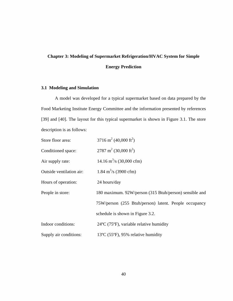
A model was developed for a typical supermarket based on data prepared by the

Food Marketing Institute Energy Committee and the information presented by references

[39] and [40]. The layout for this typical supermarket is shown in Figure 3.1. The store

description is as follows:

Store floor area: 3716 m2 (40,000 ft2)

Conditioned space: 2787 m2 (30,000 ft2)

Air supply rate: 14.16 m3/s (30,000 cfm)

Outside ventilation air: 1.84 m3/s (3900 cfm)

Hours of operation: 24 hours/day

People in store: 180 maximum. 92W/person (315 Btuh/person) sensible and

75W/person (255 Btuh/person) latent. People occupancy

schedule is shown in Figure 3.2.

Indoor conditions: 24ºC (75ºF), variable relative humidity

Supply air conditions: 13ºC (55ºF), 95% relative humidity

41

Figure 3.1: Layout of typical supermarket.

The installed refrigerated display cases capacity were set as follow: medium temperature

horizontal single shelf display at [73m (240ft)], medium temperature vertical multi-shelf

display at [73m (240ft)] and low temperature closed door within a reach-in of [91m

(300ft)].

42

1 3 5 7 9 11 13 15 17 19 21 230

20

40

60

80

100

120

140

160

180

200

Hour

Num

ber o

f peo

ple

Figure 3.2: Schedule of people occupancy in supermarket model.

The hourly outdoor weather condition for Tampa, Florida is averaged for the

years 2000-2010 [41] and illustrated in Figure 3.3. The hourly moisture balance was

performed on the supermarket for a typical 24-hour day and averaged over the years

2000-2010. The annual effect can be obtained from the averaged weather data. The

moisture balance, in terms of the latent energy balance is given by the following

equation:

casedisplay bakerymeatproducepeopleinfilspace QLQLQLQLQLQLQL −+++=+ (9)

43

0 5 10 15 20 2540

50

60

70

80

90

Hour

Tem

pera

ture

(F) a

nd re

lativ

e hu

mid

ity (%

) January

0 5 10 15 20 2540

50

60

70

80

90

Hour

Tem

pera

ture

(F) a

nd re

lativ

e hu

mid

ity (%

) February

0 5 10 15 20 2540

50

60

70

80

90

Hour

Tem

pera

ture

(F) a

nd re

lativ

e hu

mid

ity (%

) March

0 5 10 15 20 2540

50

60

70

80

90

Hour

Tem

pera

ture

(F) a

nd re

lativ

e hu

mid

ity (%

) April

Temperature (F)Relative humidity (%)

0 5 10 15 20 2540

50

60

70

80

90

Hour

Tem

pera

ture

(F) a

nd re

lativ

e hu

mid

ity (%

) May

0 5 10 15 20 2540

50

60

70

80

90

Hour

Tem

pera

ture

(F) a

nd re

lativ

e hu

mid

ity (%

) June

0 5 10 15 20 2540

50

60

70

80

90

Hour

Tem

pera

ture

(F) a

nd re

lativ

e hu

mid

ity (%

) July

0 5 10 15 20 2540

50

60

70

80

90

Hour

Tem

pera

ture

(F) a

nd re

lativ

e hu

mid

ity (%

) August

0 5 10 15 20 2540

50

60

70

80

90

Hour

Tem

pera

ture

(F) a

nd re

lativ

e hu

mid

ity (%

) September

0 5 10 15 20 2540

50

60

70

80

90

Hour

Tem

pera

ture

(F) a

nd re

lativ

e hu

mid

ity (%

) October

0 5 10 15 20 2540

50

60

70

80

90

Hour

Tem

pera

ture

(F) a

nd re

lativ

e hu

mid

ity (%

) November

0 5 10 15 20 2540

50

60

70

80

90

Hour

Tem

pera

ture

(F) a

nd re

lativ

e hu

mid

ity (%

) December

Figure 3.3: Annual average hourly outdoor temperature and relative humidity in variation Tampa, Florida (2000-2010).

44

The moisture balance states that the net moisture loss due to the building envelope

and the operation of the air-conditioning equipment is balanced by the net production of

moisture within the supermarket. The terms of the moisture equation are calculated from

the following equations and thermal conditions:

QLspace = 3010 qspace (wspace − wsupply ) (10)

QLinfil = 3010 qinfil (wspace − woutside) (11)

NP 075.0people =QL (12)

Btu/hr 1400kW 4103.0produce ==QL (constant for 24 hours) (13)

Btu/hr 1400kW 4103.0meat ==QL (from 5am to 10am) (14)

Btu/hr 12000kW 517.3bakery ==QL (from 5am to 10pm) (15)

where,

qinfil = 44.5NP - 0.095NP2 +10−4 NP3( )∆Pbuild

qspace =14.16 m3/s = 30,000 cfm

OHin 0.16 OH mm 02.4 22 ==∆ buildP

The major component of the display case model (QLdisplay case), is given by the air

curtain. A strong heat and mass transfer exist within the air curtain as it separates the

internal and external environment as shown in Figure 3.4. Figure 3.4 illustrates a vertical

multi-shelf refrigerated display case, a typical horizontal single shelf refrigerated display

case and standard closed door reach-in refrigerated case. The correlation of Ge and

Tassou [26] was used for the air curtain of the refrigerated display cases. The four main

parameters that affect the heat transfer of air curtain are the store air enthalpy, the dry-

bulb temperature of the air curtain supply, display case air temperature or the air

45

temperature differential between the display case and the curtain supply, and air curtain

properties such as: air curtain velocity and length. The air curtain thickness effect is

included as part of the curtain velocity, which is generally presented by the mass flow

rate. In the current work, the effect of air curtain length is ignored by the assumption of a

unit length. In addition, Ge and Tassou [26] correlation was used to predict the heat

transfer of horizontal and closed door reach-in refrigerated display cases and vertical

multi-shelf refrigerated display cases. This is validated as part of the sensitivity analysis.

The design specifications of Howell and Adams [13] for different display cases are

shown in Table 3.1. In general, the following correlation was used to predict the heat

transfer of air curtain for any display case:

( ) ( ) ( ) amcTThcTTcTTchchcQ ][ 6casespace5case42

case3space22space1curtainair +∆++∆++∆+++= (16)

where,

)86.13.2501(0.1 spacespacespacespace TwTh ++= (17)

and c1–c6 are constants, which can be correlated from the simulation results of Ge and

Tassou [26]. The correlated results of c1–c6 constants are shown in Table 3.2.

46

(a) (b) (c)

Figure 3.4: Typical refrigerated display cases: (a) Vertical multi shelf (b) Horizontal single shelf (c) Closed door reach-in [28].

Table 3.1: Design specifications for different types of refrigerated display case [13].

Case Type Orientation Case length m (ft)

Case Temp ºC (ºF)

Air curtain supply Temp ºC (ºF)

Air curtain velocity m/s

(fpm)

Air curtain

thickness m (in)

Medium Temp Single shelf

Horizontal 73 (240)

4.4 (24)

2 (35)

0.56 (110)

0.102 (4.0)

Medium Temp Multi-shelf

Vertical 73 (240)

3 (37)

0 (32)

1.32 (260)

0.114 (4.5)

Low Temp Reach-in

Vertical 91 (300)

-2 (29)

-4.4 (24)

0.68 (133)

0.076 (3.0)

Table 3.2: The correlated constants c1-c6 [26].

c1 c2 c3 c4 c5 c6 -0.180 303.180 -0.781 216.309 -0.448 509.975

ASHRAE [42] gave the percentage of latent load for each type of refrigerated

display case; 12% for single shelf, 19% for multi-shelf and reach-ins respectively. These

values take in account the performance of display cases with a store relative humidity

Air curtain Air curtain

Air curtain

47

maintained of 55%. The latent load percentage values for each type of refrigerated

display case decreases at lower relative humidity and affects the simulated store relative

humidity. However, the latent load percentage values for each type of refrigerated display

case are taken as the maximum to prevent any frost formation and maintain the desired

temperature of products. In this work, MATLAB [43] software was used to simulate the

latent heat balance inside the supermarket. Steady state simulations were carried out on

an hourly basis for the typical day in each month using the averaged annual data obtained

from [41] using the weather conditions of Tampa, Florida during the period of 2000-

2010. The average of these data are illustrated in Figure 3.3. The store temperature is

maintained at 24ºC (75ºF). The hourly moisture balance, equation (9), was used along

with the air curtain heat equation, equation (16), and resulted in a relative humidity

profile for the typical day inside of the store. Figure 3.5 shows a flow-diagram of how the

simulation works using input data. The output includes an hourly store relative humidity

for a typical day of each month of the year.

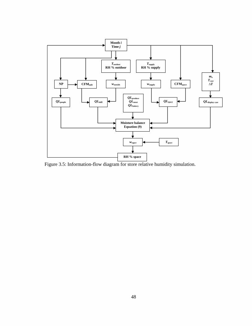
48

Figure 3.5: Information-flow diagram for store relative humidity simulation.

Month i Time j

NP CFMinfil

Toutdoor RH % outdoor

Tsupply RH % supply

woutside wsupply CFMspace

ma Tcase ∆T

QLpeople QLinfil QLspace QLdisplay case

QLproduce QLmeat

QLbakery

Moisture balance Equation (9)

wsapce Tspace

RH % space

49

3.2 Simulation Results

The results from the supermarket model simulations were run for the typical 24-

hour day for a year. The results present the store relative humidity each hour for typical

day each month. Figure 3.6 illustrates an hourly plot of store relative humidity for typical

year in Tampa, Florida. The store relative humidity remains in the range of 40-60% from

January till May and from October till December. During the summer season from June

till September, the store relative humidity increases above 60% during noon times. This

is obvious because of the hot and humid weather in Tampa, Florida during noon times.

The hourly values for the all months simulated have been averaged separately and

are presented in Table 3.3. The monthly store relative humidity in Table 3.3 remains in

the range of 40-60%. These results are dependent on the assumptions made for the

supermarket model. However, these results appear to be typical for a supermarket with

air-conditioning located in a weather condition similar to Tampa, Florida. The variation

expected in the store relative humidity would be in the range of 40-60% for hot and

humid climates. The results in Table 3.3 should be considered of what is anticipated in a

supermarket rather than using a design store relative humidity of 55%. Thus, changes in

the refrigerated display case energy can be estimated for increases or decreases in store

relative humidity, and that resulted in changes in the operation of the supermarket air-

conditioning system. This will be analyzed later on in the energy consumption changes

section.

50

0 5 10 15 20 250

20

40

60

80

Hour

rela

tive

hum

idity

(%)

January

0 5 10 15 20 250

20

40

60

80

Hour

rela

tive

hum

idity

(%)

February

0 5 10 15 20 250

20

40

60

80

Hour

rela

tive

hum

idity

(%)

March

0 5 10 15 20 250

20

40

60

80

Hour

rela

tive

hum

idity

(%)

April

0 5 10 15 20 250

20

40

60

80

Hour

rela

tive

hum

idity

(%)

May

0 5 10 15 20 250

20

40

60

80

Hour

rela

tive

hum

idity

(%)

June

0 5 10 15 20 250

20

40

60

80

Hour

rela

tive

hum

idity

(%)

July

0 5 10 15 20 250

20

40

60

80

Hour

rela

tive

hum

idity

(%)

August

0 5 10 15 20 250

20

40

60

80

Hour

rela

tive

hum

idity

(%)

September

0 5 10 15 20 250

20

40

60

80

Hour

rela

tive

hum

idity

(%)

October

0 5 10 15 20 250

20

40

60

80

Hour

rela

tive

hum

idity

(%)

November

0 5 10 15 20 250

20

40

60

80

Hour

rela

tive

hum

idity

(%)

December

Figure 3.6: Hourly relative humidity for model store for typical year in Tampa, Florida.

51

Table 3.3: Average store relative humidity for supermarket model simulated at 24ºC (75ºF) for each month for Tampa, Florida.

Month Average relative humidity inside store (%)

January February March April May June July

August September

October November December

43.72 44.51 46.66 48.24 52.57 57.40 58.87 59.28 57.41 52.08 47.48 44.92

52

3.3 Sensitivity Analysis

The performance of the model representing the supermarket refrigeration system

needs to be evaluated for different outdoor conditions each month for the whole year. The

incorporation of air curtain correlation for latent heat calculation of the refrigerated

display cases has been evaluated by a comparison with pervious simulation model [39]

and existing experimental data [18] for the weather conditions of Tampa, Florida. The

supermarket model developed by [39] has the same description of the current model,

however, the current model includes the effect of store relative humidity on refrigerated

display cases assigned in the moisture balance. Also, it can simulate the store relative

humidity on an hourly basis. Figures 3.7 and 3.8 show comparison of the hourly store

relative humidity of [39] and the current model for the months of January and August,

respectively. In January, the relative humidity inside the store exhibits stable behavior for

the current model. This is because the current model has a precise representation of the

display cases, and they are affected by the store relative humidity. The results of the

current model are comparable with model [39]. The discrepancy is because the input

weather data used for the model in [39] is interpolated and extrapolated, while it is taken

hour by hour in the current model. In the month of August, Figure 3.8, there is an

increase in the store relative humidity around noon. This is due to the high temperature

and high relative humidity of the weather during summer season. However, the results of

the current model are comparable with model [39].

53

1 3 5 7 9 11 13 15 17 19 21 2320

25

30

35

40

45

50

55

60

65

70

Hour

Rel

ativ

e hu

mid

ity (%

)

Model [39]Current model

Figure 3.7: Comparison of hourly relative humidity for [39] and supermarket model for

month of January.

1 3 5 7 9 11 13 15 17 19 21 2320

30

40

50

60

70

80

90

Hour

Rel

ativ

e hu

mid

ity (%

)

Model [39]Current model

Figure 3.8: Comparison of hourly relative humidity for [39] and supermarket model for

month of August.

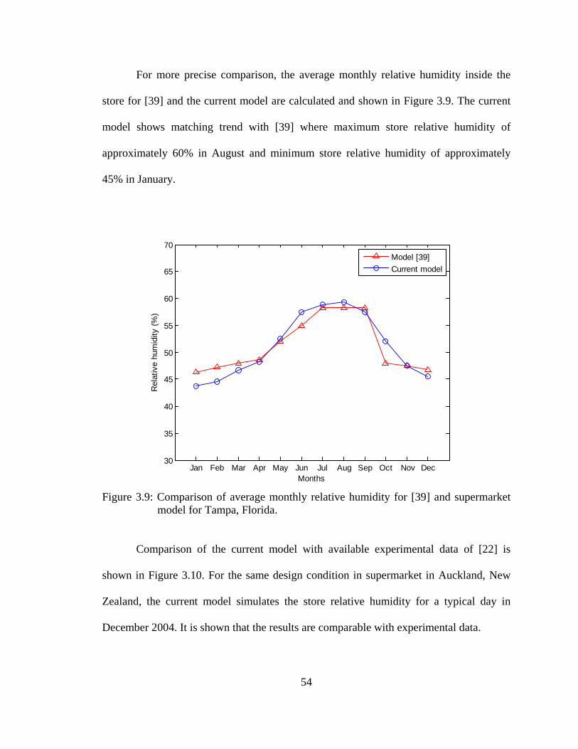
54

For more precise comparison, the average monthly relative humidity inside the

store for [39] and the current model are calculated and shown in Figure 3.9. The current

model shows matching trend with [39] where maximum store relative humidity of

approximately 60% in August and minimum store relative humidity of approximately

45% in January.

Jan Feb Mar Apr May Jun Jul Aug Sep Oct Nov Dec30

35

40

45

50

55

60

65

70

Months

Rel

ativ

e hu

mid

ity (%

)

Model [39]Current model

Figure 3.9: Comparison of average monthly relative humidity for [39] and supermarket

model for Tampa, Florida.

Comparison of the current model with available experimental data of [22] is

shown in Figure 3.10. For the same design condition in supermarket in Auckland, New

Zealand, the current model simulates the store relative humidity for a typical day in

December 2004. It is shown that the results are comparable with experimental data.

55

1 3 5 7 9 11 13 15 17 19 21 2320

25

30

35

40

45

50

55

60

Hour

Rel

ativ

e hu

mid

ity (%

)

Experimental data [22]Current model

Figure 3.10: Comparison of relative humidity for experimental data [22] and supermarket

model for a typical day in Auckland, New Zealand in December 2004.

Figure 3.11 shows a comparison of the current model with the experimental data

of [18]. Figure 10 shows the maximum, minimum and averaged store relative humidity

for a typical store located in Tampa, Florida. There is an increase in the store relative

humidity during the summer season beginning in May and ending in September. The

current model has a trend in the range of experimental data. Also, the percentage values

assumed for latent heat calculation for the refrigerated display cases are maximum, so for

more precise results, they need to be varied with store relative humidity. Overall, the

representation of display cases brought by the air curtain energy equation (16) is feasible

to be used in the supermarket model for latent heat calculations.

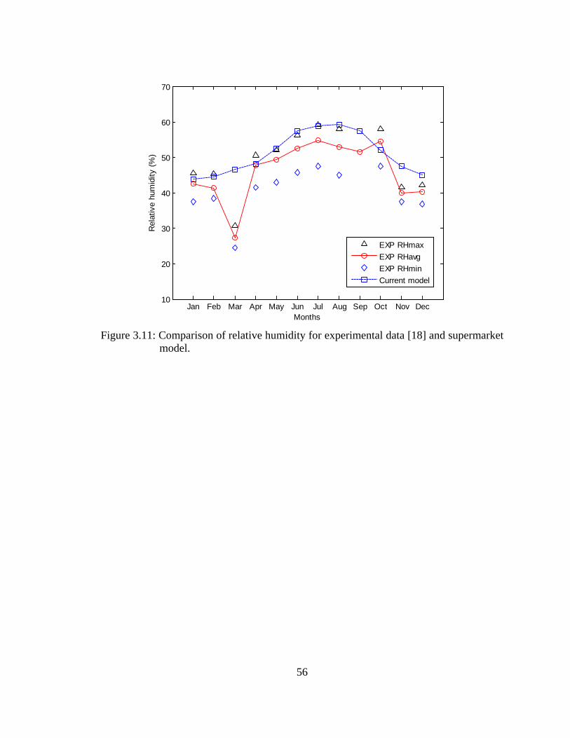
56

Jan Feb Mar Apr May Jun Jul Aug Sep Oct Nov Dec10

20

30

40

50

60

70

Months

Rel

ativ

e hu

mid

ity (%

)

EXP RHmaxEXP RHavgEXP RHminCurrent model

Figure 3.11: Comparison of relative humidity for experimental data [18] and supermarket

model.

57

3.4 Energy Consumption Analysis

The modern supermarket is the greatest consumer for refrigeration energy within

the commercial sector. In the United States, the electrical consumption in supermarkets

presents 2.3% of the national electric use, and 50% of the total retail store energy is

consumed by the refrigerated display cases and air-conditioning systems [42]. The

relationship between the store HVAC and the refrigeration is very important in terms of

the overall energy consumption of the supermarket. Howell [13-15] developed several

procedures to calculate the savings in store energy requirement by the knowledge of the

indoor store relative humidity distribution during the year. He showed the influence of

the indoor relative humidity on the refrigerated display case energy consumption. The

method developed will be used in this work to evaluate the effect of store relative

humidity on display case energy requirements. These energy requirements were divided

into three components: energy required by the case refrigeration, energy required by anti-

sweat heaters, and energy required for defrost. The store relative humidity affects all

three of these components. Each of these refrigerated display case loads were evaluated

on a percent change basis, compared to operation at relative humidity of 55%, and are

given by the following equations [13]:

QRQRHTP /= (18)

DFDFRHDP /= (19)

ASWASWRHAP /= (20)

where,

TP: ratio of display case refrigeration energy requirement when operated at a relative

humidity other that 55%.

58

QRH: display case refrigeration energy requirement at a given relative humidity.

QR: display case refrigeration energy requirement at the design value of relative humidity

of 55%.

DP: ratio of display case defrost energy requirements when operated at a relative

humidity other than 55%.

DFRH: defrost energy requirement for the display case at a given relative humidity.

DF: defrost energy requirement for the display case at the design value of relative

humidity of 55%.

AP: ratio of display case anti-sweat heater load when operated at a relative humidity

other than 55%.

ASWRH: anti-sweat heater energy requirement for the display case at a given relative

humidity.

ASW: anti-sweat heater energy requirement for the display case at the design value of

relative humidity of 55%.

Howell [14] evaluated the values for TP and DP when the store temperature was

kept at 24ºC (75ºF). These values are listed in Tables 3.4 and 3.5, and can be used for a

wide variation in types of display cases as well as a full variation of case sizes and

operating conditions. TP and DP values for multi-shelf refrigerated vertical display cases

are listed in Table 3.4, while Table 3.5 lists the values for single-shelf horizontal display

cases. Values for AP are evaluated also for different display case temperatures as shown

in Table 3.6.

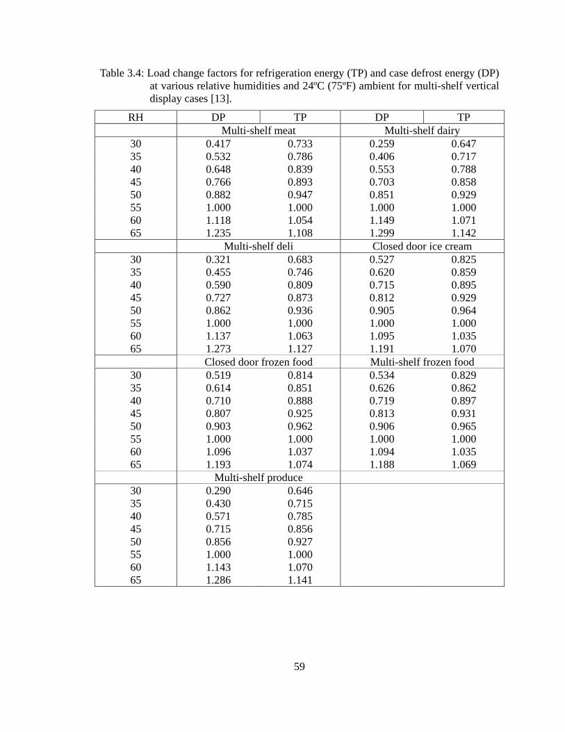
59

Table 3.4: Load change factors for refrigeration energy (TP) and case defrost energy (DP) at various relative humidities and 24ºC (75ºF) ambient for multi-shelf vertical display cases [13].

RH DP TP DP TP Multi-shelf meat Multi-shelf dairy

30 0.417 0.733 0.259 0.647 35 0.532 0.786 0.406 0.717 40 0.648 0.839 0.553 0.788 45 0.766 0.893 0.703 0.858 50 0.882 0.947 0.851 0.929 55 1.000 1.000 1.000 1.000 60 1.118 1.054 1.149 1.071 65 1.235 1.108 1.299 1.142 Multi-shelf deli Closed door ice cream

30 0.321 0.683 0.527 0.825 35 0.455 0.746 0.620 0.859 40 0.590 0.809 0.715 0.895 45 0.727 0.873 0.812 0.929 50 0.862 0.936 0.905 0.964 55 1.000 1.000 1.000 1.000 60 1.137 1.063 1.095 1.035 65 1.273 1.127 1.191 1.070 Closed door frozen food Multi-shelf frozen food

30 0.519 0.814 0.534 0.829 35 0.614 0.851 0.626 0.862 40 0.710 0.888 0.719 0.897 45 0.807 0.925 0.813 0.931 50 0.903 0.962 0.906 0.965 55 1.000 1.000 1.000 1.000 60 1.096 1.037 1.094 1.035 65 1.193 1.074 1.188 1.069 Multi-shelf produce

30 0.290 0.646 35 0.430 0.715 40 0.571 0.785 45 0.715 0.856 50 0.856 0.927 55 1.000 1.000 60 1.143 1.070 65 1.286 1.141

60

Table 3.5: Load change factors for refrigeration energy (TP) and case defrost energy (DP) at various relative humidities and 24ºC (75ºF) ambient for single shelf horizontal display cases [13].

RH DP TP DP TP Single-shelf meat Single-shelf frozen

31 0.465 0.799 0.553 0.853 34 0.536 0.826 0.612 0.872 38 0.609 0.853 0.673 0.892 41 0.684 0.881 0.736 0.912 44 0.760 0.910 0.799 0.933 48 0.838 0.939 0.865 0.955 51 0.918 0.968 0.931 0.978 55 1.000 1.000 1.000 1.000 58 1.083 1.031 1.069 1.021 62 1.169 1.064 1.141 1.044 Single-shelf ice cream Single-shelf produce

31 0.558 0.865 0.363 0.774 34 0.617 0.881 0.448 0.803 38 0.678 0.900 0.535 0.834 41 0.739 0.919 0.624 0.866 44 0.802 0.939 0.715 0.897 48 0.867 0.958 0.807 0.929 51 0.932 0.979 0.902 0.965 55 1.000 1.000 1.000 1.000 58 1.068 1.022 1.099 1.035 62 1.139 1.044 1.201 1.070

Table 3.6: Load change factor (AP) for anti-sweat energy requirements for all types of display cases at 24ºC (75ºF) ambient [13].

Display case temperature Store RH (%) 5ºC (41ºF) 3ºC (37ºF) -2ºC (29ºF) -22ºC (-7ºF)

65 1.28 1.23 1.16 1.07 60 1.15 1.12 1.09 1.04 55 1.00 1.00 1.00 1.00 50 0.84 0.87 0.91 0.96 45 0.67 0.73 0.81 0.91 40 0.48 0.58 0.70 0.86 35 0.27 0.41 0.57 0.81

61

In order to calculate the savings in energy in the operation of the display cases, it

is necessary to establish its standard energy consumption for the refrigeration energy,

defrost energy and anti-sweat heater energy. The defrost energy and anti-sweat heaters

energy are estimated by Howell and Adams [13] and given in Table 3.7. Equation (16) is

used to calculate the refrigeration energy for the display cases at 24ºC store temperature

and relative humidity of 55%. The medium temperature single shelf horizontal units of

length 240 ft (73m) has calculated refrigeration energy of 628 Btu/hr-ft and assumed to

have an energy efficiency ratio (EER) of 8 Btu/Wh. The medium temperature multi-shelf

vertical units of length 240 ft (73m) has calculated refrigeration energy of 1735 Btu/hr-ft

and assumed to have an energy efficiency ratio (EER) of 7 Btu/Wh. The low temperature

closed door reach-in units of length 300 ft (91m) has calculated refrigeration energy of

536 Btu/hr-ft and assumed to have an energy efficiency ratio (EER) of 6 Btu/Wh. Thus,

kW demand and the kWh per month can be calculated as shown in Table 3.7 for the three

display cases. Howell and Adams [13] gave approximate values for defrosts energy and

anti-sweat heaters energy as shown in Table 3.7. They are taken at the rated store relative

humidity of 55%. The number of defrosts varied from 2 to 4 per day and consumed

16,667 kWh per month and the total anti-sweat heater load was 23.4 kW which consumed

16,850 kWh per month. The annual energy load for the refrigeration, defrost and anti-

sweat heaters is about 1,311,000 kWh. Normally, this load is about 70% of the

supermarket’s total annual energy consumption.

62

Table 3.7: Display case refrigeration energy for simulated store at 24ºC (75ºF) and 55% relative humidity.

Case Type Orientation Case length m (ft)

Case Temp ºC (ºF)

Btu/ hr-ft

kW (Btu/hr)

EER kW demand

kWh/ month

Medium Temp

Single shelf

Horizontal 73 (240)

4.4 (24)

628 44 (150,906)

8 18.86 13,580

Medium Temp

Multi-shelf

Vertical 73 (240)

3 (37)

1735 122 (416,600)

7 59.50 42,840

Low Temp

Reach-in

Vertical 91 (300)

-2 (29)

536 47 (160,738)

6 26.79 19,289

Total 237 (780)

-- -- -- -- 105.15 75,709

Defrost 2 to 4 per day 16,667 Anti-sweat

heaters 23.4 kW 16,850

In order to evaluate savings in display case energy with reductions in ambient

store relative humidity it is necessary to determine TP, DP and AP at different store

relative humidities. These three factors or modifiers can then be used with the energy

loads given in Table 3.7 to estimate energy requirements at the different store relative

humidity. The average monthly relative humidity for supermarket model is determined

and listed in Table 3.3. Assuming each month has the same number of days, the twelve

months are averaged and resulting in an annual average store relative humidity of 51.1%.

This seems to be a feasible value for the Tampa, Florida weather climate. Since display

cases are designed for 55% ambient relative humidity, the actual annual energy

requirement for the display cases for this supermarket model would be less than 1.31

million kWh as previously calculated.

63

To calculate the energy savings for these display cases, the three energy factors or

modifiers are determined for the new store relative humidity of 51.1%. This is done using

the information in Tables 3.4, 3.5 and 3.6. Values for TP, DP and AP are found for

average annual store relative humidities of 51.1%, 45%, 40%, and 35% and listed in

Table 3.8 for the three display cases. The values for TP, DP and AP are 1.0 for 55% RH.

This is the reference point for upcoming results. Using the display case energy

requirements at 55% relative humidity in Table 3.7, and energy modifiers listed in Table

3.8, annual energy requirements at various store relative humidities are estimated in

Table 3.9. The total display cases energy load is separated into refrigeration energy,

defrost energy and anti-sweat energy so that it can be compared with the actual situations.

Notice from Table 3.8 that reducing the store relative humidity results in reduction in the

total display cases energy requirements as mentioned previously.

Table 3.8: Display case energy modifiers for various average annual store relative humidities.

Average annual store relative humidity

51.1% RH

45% RH

TP DP AP TP DP AP Medium Temp Single shelf 0.966 0.904 0.882 0.905 0.738 0.688 Medium Temp Multi-shelf 0.945 0.884 0.899 0.858 0.703 0.730

Low Temp Reach-in 0.959 0.908 0.930 0.893 0.766 0.810 Average annual store relative

humidity 40% RH 35% RH

TP DP AP TP DP AP Medium Temp Single shelf 0.855 0.594 0.510 0.811 0.470 0.312 Medium Temp Multi-shelf 0.788 0.553 0.580 0.717 0.406 0.410

Low Temp Reach-in 0.839 0.648 0.700 0.786 0.532 0.570

64

Table 3.9: Display cases annual energy requirements at various store relative humidities. 55% RH 51.1% RH 45% RH 40% RH 35% RH

Refrigeration, kWh 908,508 864,908 795,260 738,682 682,649 Defrost, kWh 200,004 179,750 147,136 119,691 93,852

Anti sweat, kWh 202,200 182,696 150,167 120,646 87,081 Total, kWh 1,310,712 1,227,354 1,092,564 979,019 863,582

The percent savings in energy for the various components as well as the total

display case energy savings for the various store relative humidities are given in Table

3.10. The base case for comparison is at store relative humidity of 51.1%. It may be

noticed from Table 3.10 that for range of store relative humidity of 35-55%, the changes

in energy requirements are approximately linear. These results show that for a 5%

reduction in store relative humidity; the refrigeration load is reduced by 6.5%, the defrost

load is reduced 15%, the anti-sweat heater load is reduced 16%, and the total display case

load is reduced 9.25%.

Table 3.10: Percentage changes in energy for various store relative humidities (percent change compared to base case at 51.1% RH).

55% RH 51.1% RH 45% RH 40% RH 35% RH Total, kWh 1,310,712 1,227,354 1,092,564 979,019 863,582 Change % +6.36 0.00 -10.98 -20.23 -29.64

Defrost, kWh 200,004 179,750 147,136 119,691 93,852 Change % +10.13 0.00 -18.14 -33.41 -47.79

Anti-sweat, kWh 202,200 182,696 150,167 120,646 87,081 Change % +9.65 0.00 -17.80 -33.96 -52.34

Refrigeration, kWh 908,508 864,908 795,260 738,682 682,649 Change % +4.80 0.00 -8.05 -14.59 -21.07

65

In order to justify the reduction in store relative humidity, the percent increase in

air-conditioning energy required to reduce the store relative humidity by 5% should be

determined. Howell [15] estimated the annual air-conditioning energy requirement

needed to maintain the store at 24ºC (75ºF) and relative humidity of 55%. They simulated

a retail store, and found that for AC unit with energy efficiency ratio of 9.5 Btu/W-hr,

and 2.812 watts cooling/watts power, the annual energy was estimated to be 478,600

kWh. When reducing the store relative humidity to 45%, the same AC unit would require

499,600 kWh, and for store relative humidity of 35%, 516,600 kWh was required. For

our designed store relative humidity of 51.1%, the AC energy required is 486,790 kWh.

Howell [15] also showed, in order to evaluate reasonable percent changes in energy for

the total supermarket, lights and appliances annual energy are required and estimated as

300,000 kWh. These data are shown in Table 3.11 to compare changes in energy

requirements at different relative humidities for each component of the store electric bill.

From Table 3.11, it can be determined that for a 5% reduction in store relative humidity,

there is about 4.82% reduction in the total store annual energy. Also, it can be determined

that for each 1% reduction in store relative humidity, there is an approximate savings in

annual store energy of 19,000 to 20,000 kWh.

66

Table 3.11: Changes in total store energy requirements at various relative humidities.

55% RH 51.1% RH 45% RH 40% RH Total display case annual energy, kWh 1,310,712 1,227,354 1,092,564 979,019 AC annual energy, kWh 478,600 486,790 499,600 508,100 Lights and appliances, annual energy, kWh 300,000 300,000 300,000 300,000 Total store annual energy, kWh 2,089,312 2,014,144 1,892,164 1,787,119 Saving realized by changing from 55% RH, kWh -- 75,168 197,148 302,193 Saving in kWh for each 1% reduction in RH, kWh -- 19,274 19,715 20,146 Percentage savings in total store energy by changing from 55% RH, % -- 3.60 9.44 14.46 Percent savings in total store energy for each 1% change in RH, % -- 0.92 0.94 0.96

Howell et al. [39] estimated the annual air-conditioning energy requirement

needed to maintain the store at 24ºC (75ºF) and relative humidity of 51.2%. They found

for a 5% reduction in store relative humidity, the display case refrigeration load reduced

by 10%, and that results in total store energy load reduction of 4.7%. Because of the

integration of store relative humidity within the air curtain correlation in the moisture

balance, the current model shows a reduction in the display case refrigeration load by

9.25% for a 5% reduction in store relative humidity, while Howell et al. [39] model had a

reduction in refrigeration load of 10%. However, the recommended relative humidity by

Howell et al. [39], and the one determined in this work are comparable. Estimated store

relative humidities by Howell et al. [39] and in the current model are 51.2% and 51.1%,

respectively. The current model shows a reduction in the total store energy load by

4.84%, while Howell et al. [39], the load was reduced by 4.7%. This explains the

sensitivity of the current model. In addition, the current model incorporate the effect of

67

store relative humidity with the refrigerated display cases assigned in the supermarket

model.

The results of the sensitivity analysis and energy analysis show that the use of air

curtain correlation is feasible to study the effect of relative humidity inside the retail

store. This has been evaluated to be used for different types of display cases such as

horizontal and closed door reach-ins type, and shows good agreement with previous

models and experimental data. Thus, it can be employed for quick design calculation and

for the simulation of different types of display cases within a supermarket model.

68

Chapter 4: Conclusions

4.1 Solar-Powered Single-Effect Absorption Cooling System

The greatest advantage of solar-powered absorption cooling system when

compared to other cooling applications is the greater the sun radiation, the greater cooling

performance that can be achieved by the solar refrigeration system. CHEMCAD model

shows good trend for cooling capacity and COP when compared with previous models. In

order to achieve higher COP, LiBr-H2O mixture is good solution to be used in solar-

powered absorption cooling system. According to the results, the cooling performance

can be varied with LiBr solution concentration. The results show for higher cooling

performance, optimized LiBr solution concentration is suggested. The effects of

evaporator and condenser pressures and varying the mass flow rate on the cooling

capacity and cooling performance are generally negligible as the results show. The

cooling performance is assessed for typical year in Tampa, Florida weather condition,

and the results show constant coefficient of performance of 0.94. Finally by considering

the problem of pollution on the planet due to the burning of fossil fuels the adoption of

solar energy to power absorption chillers, even with marginal economic benefits, should

not be underestimated.

69

4.2 Modeling of Supermarket Refrigeration/HVAC System for Simple Energy

Prediction

The integration of air curtain with moisture balance for supermarket model is

necessary in order to assess the effect of reduced store relative humidity on display case

energy requirements. So, thermodynamic analysis was used to simulate supermarket

refrigeration/HVAC system using MATLAB software. For the simulated supermarket

model described in this work with different types of refrigerated display cases, and

located in a hot and humid weather such as Tampa, Florida, the annual average

supermarket relative humidity was found to be 51.1%. This simulated store relative

humidities were found to be in the range between 40% and 60% during the model year.

The results show good agreement with previous model, and the experimental data

validates the proposed model. The effect of indoor space conditions on supermarket

energy consumption is studied. It is shown that for a 5% reduction in store relative

humidity that the display case refrigeration load is reduced by 9.25%, and that results in

total store energy load reduction of 4.84%. These results evaluated the integration of air

curtain correlation for quick design calculation and for the simulation of different types

of display cases within a supermarket model. These results, which are not generally

known for typical supermarkets in hot and humid climates will now allow the designer of

the supermarket to simply and quickly determine typical store relative humidity so that

savings in display case operation and total store energy load are correctly estimated.

70

4.3 Recommendations for Future Research

In the first problem, Lithium bromide-water mixture was used as the working

fluid for the solar absorption cooling system. This mixture shows quite good performance

for Tampa, Florida weather condition. For future work, it is recommended to study the

performance for different types of mixtures for optimum cooling performance. It is also

recommended that the design specification for each component of the system i.e

generator, evaporator, condenser, and absorber to be taken based on physical data. This

will count for the number of tubes of the heat exchanger. The coefficient of performance

will be varied with the overall heat transfer coefficient of the heat exchangers.

The effect of store relative humidity was investigated inside a typical

supermarket in Tampa, Florida. The integration of store relative humidity with the

display cases (QLdisplay case) within the moisture balance equation was highly effecting the

energy consumption of the retail store. Finding new correlations for the other parameters

of the moisture balance equation, i.e., QLproduce, QLmeat, and QLbakery, gives more precise

results for the energy consumed inside the retail store with changing the store relative

humidity. It is also recommended to modify the model to be working for different

weather conditions rather than hot and cold climate as Tampa, Florida. In addition, the

model can be modified for different supermarket layouts.

71

References

[1] ASHRAE Handbook of Fundamentals, ASHRAE, Atlanta, USA, 1997. [2] Wilbur, P.J., and Mitchell, C.E., “Solar absorption air conditioning alternatives”,

Solar Energy, vol. 17, no. 3, pp. 193-199, 1975. [3] Li, Z.F., and Sumathy, K., “Simulation of a solar absorption air conditioning

system”, Energy Conversion and Management, vol. 42, no. 3, pp. 313-327, 2001. [4] Li, Z.F., and Sumathy, K., “Experimental studies on a solar powered air

conditioning system with partitioned hot water storage tank”, Solar Energy, vol. 71, no. 5, pp. 285-297, 2001.

[5] Florides, G.A., Kalogirou, S.A., Tassou, S.A., and Wrobel, L.C., “Modelling and

simulation of an absorption solar cooling system for Cyprus”, Solar Energy, vol. 72, no. 1, pp. 43-51, 2002.

[6] Atmaca, I., and Yigit, A., “Simulation of solar-powered absorption cooling

system”, Renewable Energy, vol. 28, no. 8, pp.1277-1293, 2003. [7] Florides, G.A., Kalogirou, S.A., Tassou, S.A., and Wrobel, L.C., “Design and

construction of LiBr-water absorption machine”, Energy Conversion & Management, vol. 44, no. 15, pp. 2483-2508, 2003.

[8] Assilzadeh, F., Kalogirou, S.A., Ali, Y., and Sopian, K., “Simulation and

optimization of a LiBr solar absorption cooling system with evacuated tube collectors”, Renewable Energy, vol. 30, no. 8, pp. 1143-1159, 2005.

[9] Mittal, V., Kasana, K.S., and Thakur, N.S., “Performance evaluation of solar

absorption cooling system of Bahal (Hatyana)”, Journal of the Indian Institute of Science, vol. 85, pp. 295-305, 2005.

[10] Sayegh, M.A., “The solar contribution to air conditioning systems for residential

buildings”, Desalination, vol. 209, vol. 1-3, pp. 171-176, 2007. [11] Balghouthi, M., Chahbani, M.H., and Guizani, A., “Feasibility of solar absorption

air condition in Tunisia”, Building and Environment, vol. 43, no. 9, pp. 1459-1470, 2008.

72

[12] Mateus, T., and Oliveira, A.C., “Energy and economic analysis of an integrated solar absorption cooling and heating system in different building types and climates”, Applied Energy, vol. 86, no. 6, pp. 949-957, 2009.

[13] Howell, R.H., and Adams, P.A., “Effects of indoor space conditions on

refrigerated display case performance”, Final report, ASHRAE-596 RP, 1991. [14] Howell, R.H., “Effects of store relative humidity on refrigerated display case

performance”, ASHRAE Transactions, vol. 99, no. 1, pp. 667-678, 1993. [15] Howell, R.H., “Calculation of humidity effects on energy requirements of

refrigerated display cases”, ASHRAE Transactions, vol. 99, no. 1, pp. 679-693, 1993.

[16] Tassou, S.A., and Datta, D., “Influence of supermarket environmental parameters

on the frosting and defrosting of vertical multideck display cabinets”, ASHRAE Transactions, vol. 105, no. 1, pp. 491-496, 1999.

[17] Orphelin, M., Marchio, D., and D’Alanzo, S.L., “Are there optimum temperature

and humidity set points for supermarkets?”, ASHRAE Transactions, vol. 105, no. 1, pp. 497-507, 1999.

[18] Rosario, L., and Howell, R.H., “Relative humidity and temperature measurement

and predictions in supermarket”, ASHRAE Transactions, vol. 107, no. 2, pp. 415-423, 2001.

[19] Kosar, D., and Dumitrescu, O., “Humidity effects on supermarket refrigerated

case energy performance: a database review”, ASHRAE Transactions, vol. 111, no. 1, pp. 1051-1060, 2005.

[20] Chen, Y.-G., and Yuan, X.-L., “Experimental study of the performance of single-

band air curtains for a multi-deck refrigerated display cabinet”, Journal of Food Engineering, vol. 69, no. 3, pp. 261-267, 2005.

[21] Smale, N.J., Moureh, J., and Cortella, G., “A review of numerical models of

airflow in refrigerated food applications”, International Journal of Refrigeration, vol. 29, no. 6, pp. 911-930, 2006.

[22] Getu, H.M., and Bansal, P.K., “Modeling and performance analyses of

evaporators in frozen-food supermarket display cabinets at low temperatures”, International Journal of Refrigeration, vol. 30, no. 7, pp. 1227-1243, 2007.

[23] Ge, Y.T., Tassou, S.A., and Hadawey, A., “Simulation of multi-deck medium

temperature display cabinets with the integration of CFD and cooling coil models”, Applied Energy, vol. 87, no. 10, pp. 3178-3188, 2010.

73

[24] Howell, R.H., Van, N.Q., and Smith, C.E., “Heat and moisture transfer through turbulent recirculated plane air curtains”, ASHRAE Transactions, vol. 82, no. 2, pp. 191-205, 1976.

[25] Howell, R.H., and Shibata, M., “Optimum heat transfer through turbulent

recirculated plane air curtains”, ASHRAE Transactions, vol. 86, no. 1, pp. 188-200, 1980.

[26] Ge, Y.T., and Tassou, S.A., “Simulation of the performance of single jet air

curtain for vertical refrigerated display cabinets”, Applied Thermal Engineering, vol. 21, no. 2, pp. 201-219, 2001.

[27] Cui, J., and Wang, S., “Application of CFD in evaluation and energy-efficient

design of air curtain for horizontal refrigerated display cases”, International Journal of Thermal Sciences, vol. 43, no. 10, pp. 993-1002, 2004.

[28] Navaz, H.K., Amin, M., Dabiri, D., and Faramarzi, R., “Past, present, and future

research toward air curtain performance optimization”, ASHRAE Transactions, vol. 111, pp. 1083-1088, 2005.

[29] Ge, Y.T., and Cropper, R., “Performance simulation of refrigerated display

cabinets operating with refrigerants R22 and R404A”, Applied Energy, vol. 85, no. 8, pp. 694-707, 2008.

[30] Klein, S.A., Duffie, J.A., and Beckman, W.A., “Transient consideration of flat-

plate solar collector”, Journal of Engineering for Power, vol. 96, no. 2, pp.109-113, 1974.

[31] The 1991-2005 national solar radiation database, National Renewable Energy

Labatory, Office of Energy and Renewable Energy, Alliance for Sustainable Energy, LLC.

[32] CHEMCAD. Version 6.1.2: Process Flow Sheet Simulator. Chemstations Inc.:

Houston, 2008. [33] Edwards, J.E., Process modeling : Selection of thermodynamic methods, P&I

Design Ltd. Process Instrumentation Consultancy & Design, 2008. [34] Peters, R., Korinth, C., and Keller, J.U., “Vapor-Liquid Equilibria in the System

NH3 + H2O + LiBr. 2.Data Correlation”, Journal of Chemical & Engineering Data, vol. 40, no. 4, pp. 775-783, 1995.

[35] Özkan, D., Agra, Ö., and Cetin, Ö. , “A comparison between refrigerants used in

air conditioning”, Proceedings of Clima 2007 wellBeing Indoors, pp. 1105-1114, REHVA World Congress, Finland, Helsinki, 2007.

74

[36] He, L.J., Tang, L.M., and Chen, G.M., “Performance prediction of refrigerant-DMF solutions in a single-stage solar-powered absorption refrigeration system at low generating temperatures”, Solar Energy, vol. 83, no. 11, pp. 2029-2038, 2009.

[37] Kalogirou, S.A., “Solar thermal collectors and applications”, Progress in energy

and Combustion Science, vol. 30, no. 3, pp. 231–295, 2004. [38] Gomri, R., “Investigation of the potential of application of single effect and

multiple effect absorption cooling systems”, Energy Conversion & Management, vol. 51, no. 8, pp. 1629-1636, 2010.

[39] Howell, R.H., Rosario, L., and Bula, A., “Effects of indoor relative humidity on

refrigerated display case performance”, Proceedings of CLIMA 2000, Brussells, Belgium, 1997.

[40] R.H. Howell, A. Bula, L. Rosario, Simulation of refrigerated display case

performance in supermarkets. Proceedings of the IASTED International Conference, pp. 173-176, Banff, Canada, 1997.

[41] Weather data for 2000-2010, Tampa international airport, Weather warehouse,

Weather Source, LLC. [42] ASHRAE Handbook of Refrigeration, ASHRAE, Atlanta, USA, 2010. [43] MATLAB. Version 7.6.0.324 (R2008a). The Mathworks Inc., Natick,

Massachusetts, USA, 2008. [44] Cooling and heating load calculation manual, prepared by ASHARE, Inc., U.S

Department of Housing and Urban Development, Office of Policy Development and Research, H-2303 RP, USA, 1980.

[45] Supermarket refrigeration assessment for the commonwealth electric company,

prepared by Foster-Miller, Inc., Final report, EPRI CU-7379, 2569-9 RP, 1991. [46] The assessment and evaluation of supermarket refrigeration in the state of New

York, Prepared by Foster-Miller, Inc., Final report, EPRI TR-100357, 2569-13 RP, 1992.

[47] Leach, M., Hale, E., Hirsch, A., and Torcellini, P., “Grocery Store 50% Energy

Savings”, Technical report, NREL/TP-550-46101, 2009. [48] Stoecker, W.F., Design of thermal systems, 2nd ed., McGraw-Hill, Inc., USA,

1980. [49] Stoecker, W.F., and Jones, J.W., Refrigeration and air conditioning, 2nd ed.,

McGraw-Hill, Inc., USA, 1982.

75

[50] Bell, A.A., HVAC : Equations, Data, and Rules of thumb. McGraw-Hill, Inc., USA, 2000.

[51] Sauer, H.J., Howell, R.H., and Coad, W.J., Principles of heating, ventilating, and

air conditioning : A textbook with design data based on the 2001 ASHRAE Handbook-Fundamentals, American Society of Heating, Refrigerating and Air-Conditioning Engineers, Inc., Atlanta, USA, 2001.

[52] McQuiston, F.C., Parker, J.D., and Spitler, J.D., Heating, ventilating, and air

conditioning: analysis and design, 6th ed., John Wiley & Sons, Inc., USA, 2005.

76

Appendices

77

Appendix A: MATLAB Code for Modeling of Supermarket Refrigeration/HVAC

System

A.1 Main M-file

%main.m

close all

clear all

clc

%given

CFMspace=30000; %cfm (4.16m^3/s)

NP_max=180; %(maximum number of people in the store)

%operations time

time=1:24;

%Specified operation month by input the number of the month (1-12)

month=1:12;

%people occupancy in supermarket (NP)

NP=[0.17*NP_max 0.17*NP_max 0.17*NP_max 0.17*NP_max 0.17*NP_max

0.17*NP_max 0.17*NP_max 0.33*NP_max 0.50*NP_max 0.50*NP_max 0.50*NP_max

1.00*NP_max 1.00*NP_max 1.00*NP_max 0.50*NP_max 0.50*NP_max 0.50*NP_max

0.50*NP_max 1.00*NP_max 1.00*NP_max 1.00*NP_max 0.67*NP_max 0.67*NP_max

0.50*NP_max];

tspace=75; %indoor space condition temperature in F, (24C)

%Plot the schedule of people occupancy in supermarket

bar(time,NP,0.5,'r')

set(gca,'XTick',1:2:24)

set(gca,'XTickLabel',{'1','3','5','7','9','11','13','15','17','19','21'

,'23'})

axis([0 25 0 200])

xlabel('Hour')

78

Appendix A: (Continued)

ylabel('Number of people')

figure

delP_build=4.02; %pressure difference of building

t_supply=55; %supply temperature in F, (13C)

fi_supply=95; %supply relative humidity of air 95%

w_supply=solve_w(t_supply,fi_supply/100); %calculate supply humidity

ratio

S=str2mat('January','February','March','April','May','June','July','Aug

ust','September','October','November','December');

%model

for j=1:length(month)

%call for outdoor temperature (F) and relative humidity (%) for

specified month

[t_outside,fi_outside]=data(j);

%Plot temperature and relative humidity profiles for all months for

averaged years (2000-2010) in Tampa,FL

subplot(3,4,j)

plot(time,t_outside,'r-o',time,fi_outside,'b-+')

axis([0 25 40 90])

xlabel('Hour')

ylabel('Temperature (F) and relative humidity (%)')

title([S(j,:)])

legend('Temperature (F)','Relative humidity (%)')

%calculate the humidity ratio for given outdoor temperature (F) and

relative humidity

for k=1:length(t_outside)

w_outside(k)=solve_w(t_outside(k),fi_outside(k)/100); % tempearture in

79

Appendix A: (Continued)

F and fi in NaN

end

for i=1:length(time)

CFMinfl(i)=(44.5*NP(i)-0.095*(NP(i))^2+1e-4*(NP(i))^3)*delP_build;

QLpeople(i)=255*NP(i);

QLproduce(i)=1400; %BTU/hr (constant for 24 hours)

if (i>=5 && i<10)

QLmeat(i)=1400; %BTU/hr (from 5am to 10am)

else

QLmeat(i)=0;

end

if (i>=5 && i<22)

QLbakery(i)=12000; %BTU/hr (from 5am to 10pm)

else

QLbakery(i)=0;

End

QLdisplay(i)=17280+68400+34200; %display cases latent loads (Btu/hr)

total1(i)=QLpeople(i)+QLproduce(i)+QLmeat(i)+QLbakery(i)-QLdisplay(i);

total2(i)=QLpeople(i)+QLproduce(i)+QLmeat(i)+QLbakery(i);

w_space(j,i)=solve_w_space(total1(i),CFMinfl(i),CFMspace,w_supply,w_out

side(i));

w_space_new(j,i)=solve_w_spacenew(total2(i),CFMinfl(i),CFMspace,tspace,

w_supply,w_outside(i));

fi_space(j,i)=solve_fi(w_space(j,i),tspace);

fi_space_new(j,i)=solve_fi(w_space_new(j,i),tspace);

fi_space_month(j,i)=fi_space(j,i); %row is the month (j) , column is

Hour (i)

80

Appendix A: (Continued)

fi_space_month_new(j,i)=fi_space_new(j,i);

end

end

%plot relative humidity for each month for both models

figure

for j=1:length(month)

subplot(3,4,j)

%Y=[fi_space_month(j,:)'.*100 fi_space_month_new(j,:)'.*100];

Y=[fi_space_month_new(j,:)'.*100];

bar(Y,0.5)

axis([0 25 0 80])

xlabel('Hour')

ylabel('relative humidity (%)')

title([S(j,:)])

%legend('old','new')

end

%average relative humidity for each month

average=mean(fi_space_month')*100;

average_new=mean(fi_space_month_new')*100;

%average monthly relative humidity inside store for old model

(original)

average_rh=[46.3 47.2 48 48.6 52 55 58.2 58.2 58.2 47.9 47.5 46.8];

%Comparison plot the monthly averaged space relative humidity for old

and new models

figure

plot(month,average_rh,'-^r')

hold on

81

Appendix A: (Continued)

plot(month,average_new,'-ob')

set(gca,'xtick',1:1:12)

set(gca,'xticklabel',str2mat('Jan','Feb','Mar','Apr','May','Jun','Jul',

'Aug','Sep','Oct','Nov','Dec'))

axis([0 13 30 70])

xlabel('Months')

ylabel('Relative humidity (%)')

%title('Comparison of relative humidity for old and new models')

legend('Model [39]','Current model')

%average monthly relative humidity inside store for (experimental)

rh_exp_max=[45.56 45.27 30.78 50.55 51.94 56.21 59.13 58.05 0 58.03

41.68 42.26];

rh_exp_avg=[42.58 41.24 27.23 47.80 49.45 52.61 54.75 52.85 51.51 54.48

39.83 40.24];

rh_exp_min=[37.54 38.41 24.45 41.43 42.94 45.74 47.38 45.08 0 47.47

37.42 36.75];

%Comparison plot the monthly averaged space relative humidity for

experimental and new model

figure

plot(month,rh_exp_max,'^k')

hold on

plot(month,rh_exp_avg,'-or')

plot(month,rh_exp_min,'db')

plot(month,average_new,'--sb')

set(gca,'xtick',1:1:12)

set(gca,'xticklabel',str2mat('Jan','Feb','Mar','Apr','May','Jun','Jul',

'Aug','Sep','Oct','Nov','Dec'))

82

Appendix A: (Continued)

axis([0 13 10 70])

xlabel('Months')

ylabel('Relative humidity (%)')

%title('Comparison of relative humidity for old and new models')

legend('EXP RHmax','EXP RHavg','EXP RHmin','Current model')

%Experimental store relative humidity (%) for display cases for 24

hours

exp_rh=[35 34 33 33 34 33 36 37 39 40 40 40 40 40 41 40 39 39 39 39 36

34 34 37];

%Comparison plot the hourly averaged space relative humidity for

experimental data and current models for month 12

figure

plot(time,exp_rh,'^r')

hold on

plot(time,fi_space_month_new(12,:).*100,'-ob')

set(gca,'XTick',1:2:24)

set(gca,'XTickLabel',{'1','3','5','7','9','11','13','15','17','19','21'

,'23'})

axis([0 25 20 60])

xlabel('Hour')

ylabel('Relative humidity (%)')

%title('Comparison of relative humidity for experimental and current

model for Month 12')

legend('Experimental data [22]','Current model')

%average hourly relative humidity inside store for Month 1 for old

model (original)

time_old=[1 4 8 10 12 16 19 22 24];

83

Appendix A: (Continued)

rh_month1=[43 45 45 46 44 48 42 47 43];

%rh_month1=[48 47 46 45 51.5 51.5 51 51 50.5 50.5 45 44 43 42 49.5 48

49 39.5 40 40 40 47 46 48];

%Comparison plot the hourly averaged space relative humidity for old

and new models for Month 1

figure

plot(time_old,rh_month1,'^r')

hold on

plot(time,fi_space_month_new(1,:).*100,'-ob')

set(gca,'XTick',1:2:24)

set(gca,'XTickLabel',{'1','3','5','7','9','11','13','15','17','19','21'

,'23'})

axis([0 25 20 70])

xlabel('Hour')

ylabel('Relative humidity (%)')

%title('Comparison of relative humidity for old and new models for

Month 1')

legend('Model [39]','Current model')

%average hourly relative humidity inside store for Month 8 for old

model (original)

time_old=[1 4 8 10 12 16 19 22 24];

rh_month8=[51.5 52.5 58 66 65 61 66 59.5 60];

%rh_month8=[51.5 51.5 52.5 52.5 57 58.5 64.5 67 69.5 70.5 58 56.5 56 55

62.5 61 61 52.5 52.5 52.5 51.5 59.5 59.5 60];

%Comparison plot the hourly averaged space relative humidity for old

and new models for Month 1

figure

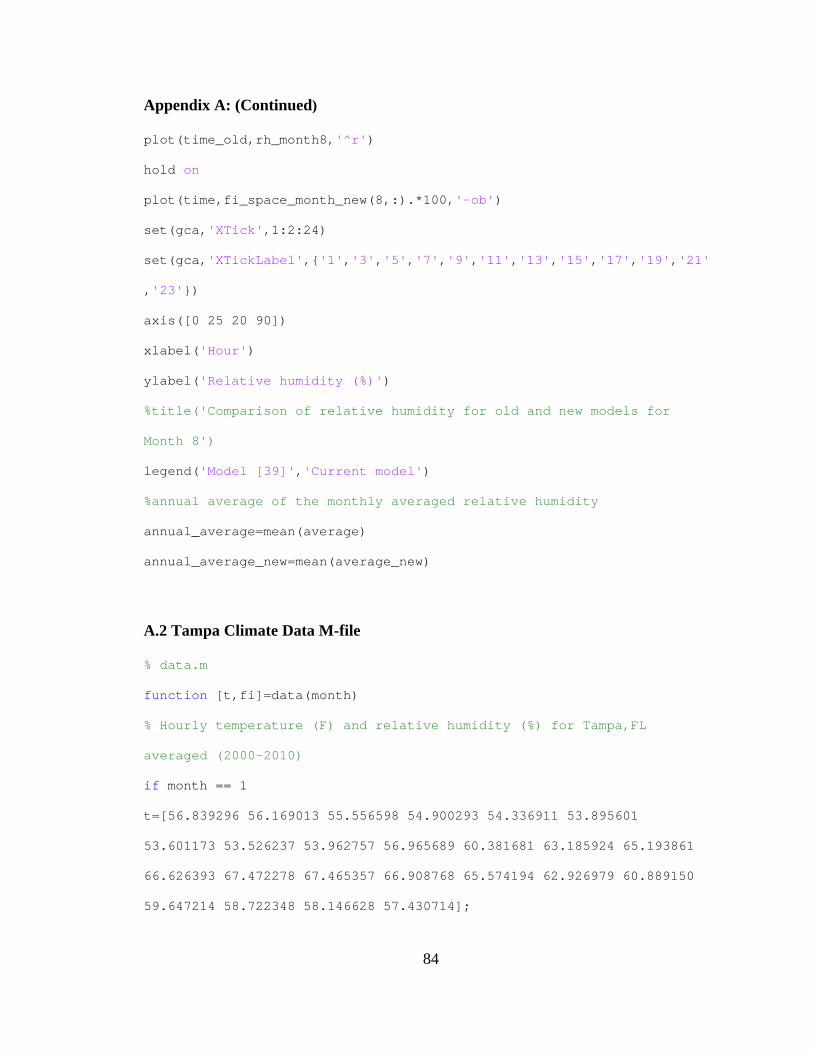
84

Appendix A: (Continued)

plot(time_old,rh_month8,'^r')

hold on

plot(time,fi_space_month_new(8,:).*100,'-ob')

set(gca,'XTick',1:2:24)

set(gca,'XTickLabel',{'1','3','5','7','9','11','13','15','17','19','21'

,'23'})

axis([0 25 20 90])

xlabel('Hour')

ylabel('Relative humidity (%)')

%title('Comparison of relative humidity for old and new models for

Month 8')

legend('Model [39]','Current model')

%annual average of the monthly averaged relative humidity

annual_average=mean(average)

annual_average_new=mean(average_new)

A.2 Tampa Climate Data M-file

% data.m

function [t,fi]=data(month)

% Hourly temperature (F) and relative humidity (%) for Tampa,FL

averaged (2000-2010)

if month == 1

t=[56.839296 56.169013 55.556598 54.900293 54.336911 53.895601

53.601173 53.526237 53.962757 56.965689 60.381681 63.185924 65.193861

66.626393 67.472278 67.465357 66.908768 65.574194 62.926979 60.889150

59.647214 58.722348 58.146628 57.430714];

85

Appendix A: (Continued)

fi=[80.879765 81.827761 82.554252 83.252199 83.555230 83.741935

83.520039 83.311828 82.492669 77.178886 70.297361 64.354839 60.364614

57.604106 56.194428 55.190029 56.346823 58.909091 64.785924 70.070381

73.354839 75.660229 77.410557 79.208798];

elseif month == 2

t=[58.917419 58.274029 57.630329 57.098095 56.673360 56.249214

56.057564 56.031134 56.986274 60.077239 63.113099 65.647450 67.545097

68.867667 69.361487 69.506538 69.182871 68.051019 66.005804 63.493014

62.028161 61.031785 60.437293 59.814514];

fi=[79.428505 80.622180 81.798762 82.657816 82.858250 83.454633

83.209003 82.704442 80.916592 74.310233 67.427004 62.347618 58.981295

56.148679 55.366099 54.737909 55.673197 57.427788 61.662313 67.455217

71.809287 74.484662 75.905732 77.531456];

elseif month == 3

t=[64.341935 63.590029 62.807918 62.262272 61.691799 61.338104

61.207380 61.048974 62.678006 65.580059 68.627273 70.885924

72.634018 73.855718 74.526344 74.828739 74.503597 73.507918 71.797654

69.454565 67.723167 66.530205 65.904985 65.280059];

fi=[76.612903 77.762463 79.416422 80.777622 81.781720 82.347019

82.287879 82.460411 79.137830 72.888563 65.615836 60.624633 57.281525

54.527859 53.336168 52.850440 53.504301 55.592375 58.782991 63.701369

68.290323 71.909091 73.715543 75.313783];

elseif month == 4

t=[68.783636 68.003636 67.178788 66.531609 65.847879 65.333030

65.053939 64.855758 65.981818 69.153187 72.237576 74.593030 76.446667

78.013333 78.986970 79.575758 79.612121 79.078788 77.926364 75.855455

73.204848 71.357273 70.296667 69.651014];

86

Appendix A: (Continued)

fi=[73.387879 75.015152 76.678788 78.695925 79.951515 81.021212

81.700000 81.893939 80.066667 72.940857 65.157576 59.569697 55.648485

52.484848 50.357576 49.181818 49.087879 49.981818 52.160606 56.090909

61.009091 66.403030 69.348485 71.192372];

elseif month == 5

t=[74.928446 74.193109 73.486510 72.841935 72.228446 71.821212

71.424340 71.338710 73.190440 75.965924 78.462564 80.555288 82.362258

83.775357 84.960117 85.650147 85.754330 85.156012 83.951613 82.265396

79.858935 77.921994 76.767155 75.882698];

fi=[74.401760 76.106256 77.941349 79.733138 81.369501 82.537732

83.454545 83.803519 80.499609 73.719746 67.307716 61.812805 57.907625

54.854154 51.794721 50.527859 50.285337 51.592375 53.706745 56.703812

61.271554 66.695015 70.190616 72.580645];

elseif month == 6

t=[78.434577 77.920522 77.363939 76.912121 76.538182 76.390606

76.153939 76.356970 78.078182 80.236970 82.287743 83.993166

85.419739 86.550303 86.874242 87.394242 87.163636 86.436061 85.170000

83.757576 81.774807 80.040909 79.467879 78.917983];

fi=[79.744932 81.119854 82.251515 83.848485 84.784013 85.387879

86.071645 85.893939 83.012121 78.333333 73.236573 68.915674 64.969488

62.136364 61.360606 60.157576 60.463636 61.690909 64.154545 66.839394

70.678474 75.221212 77.139812 78.885162];

elseif month == 7

t=[79.617595 79.194721 78.756970 78.369912 78.016051 77.897595

77.802522 77.831085 79.216716 81.296667 83.116256 84.585711 85.661848

86.400587 87.034897 86.931271 86.723167 86.082698 85.172141 83.936364

82.631085 81.216129 80.581525 80.039883];

87

Appendix A: (Continued)

fi=[80.451613 81.806452 83.056989 84.388856 85.502737 85.928446

86.118182 86.378299 84.052786 79.324242 75.203324 71.731419 68.896383

66.903324 65.070381 64.390323 64.545455 65.909091 67.501466 70.219941

72.923754 76.117302 77.829912 79.401760];

elseif month == 8

t=[79.853666 79.438123 79.013196 78.514370 78.220528 77.960704

77.805279 77.769824 78.718524 81.111378 83.233969 84.907038 85.948788

86.851026 87.202170 87.270459 87.191750 86.789189 85.776246 84.284751

82.606452 81.460117 80.705572 80.263343];

fi=[81.489736 82.478006 83.604106 85.029326 86.190616 86.923754

87.351906 87.332063 85.949267 80.991691 75.802444 71.856305 69.062561

66.868035 65.316227 65.066667 65.034506 65.742131 67.278592 70.284457

73.806452 76.909091 79.126100 80.234604];

elseif month == 9

t=[78.298182 77.825152 77.261672 76.819216 76.439613 76.150000

75.999091 75.893511 76.343939 78.784420 81.278485 83.286970

84.937367 85.933030 86.741515 87.056364 86.888401 86.183762 84.984545

83.180909 80.982194 79.987900 79.279969 78.727576];

fi=[81.403030 82.693939 84.267189 85.481923 86.504702 87.221212

87.396970 87.605538 86.778788 81.482445 75.118182 70.257576 66.217973

63.300000 61.427273 60.672727 60.864890 61.934796 64.115152 67.821212

72.796552 75.656113 77.664890 79.366667];

elseif month == 10

t=[73.074927 72.263675 71.594064 70.947952 70.403069 70.055142

69.816882 69.690792 69.888671 72.544839 75.804454 78.523063 80.636843

81.917234 82.740313 83.145637 83.200860 82.391271 80.854076 78.481565

76.491281 75.199531 74.392405 73.649218];

88

Appendix A: (Continued)

fi=[77.935679 79.780743 81.179391 82.374558 83.533529 84.249169

84.491202 84.612610 84.093842 78.773021 71.175785 64.893976 60.070772

57.219355 55.482307 54.148953 53.815957 55.049267 58.194428 63.174032

68.167351 71.943011 74.392278 76.217400];

elseif month == 11

t=[64.736729 63.867273 63.185455 62.612957 62.166667 61.873030

61.672424 61.640084 63.337273 66.920000 70.384556 72.873636 74.688182

75.729478 76.066625 76.100303 75.357273 73.695789 70.936061 69.068422

67.882424 66.916364 66.145977 65.344692];

fi=[78.343365 80.027273 81.378788 82.298224 83.087879 83.375758

83.475758 83.048589 80.009091 72.857576 65.392163 60.772727 57.281818

55.232393 54.293939 53.906061 55.286729 58.381714 64.357576 68.968652

72.151515 74.427273 76.129781 77.261129];

elseif month == 12

t=[59.506940 58.854751 58.069355 57.630332 57.152364 56.789335

56.667380 56.621994 57.135327 59.902561 62.989736 65.618182

67.589257 68.779179 69.518397 69.697243 69.159756 67.615357 65.169892

63.501760 62.384457 61.514858 60.703284 60.048573];

fi=[80.064223 80.994330 81.860508 82.613783 83.263033 83.479277

83.324633 83.105572 81.550342 75.967253 69.495601 64.672825 60.962170

58.762463 57.350342 56.649756 57.908895 60.498729 66.042522 70.260997

73.143695 75.525024 77.605474 78.668328];

%fi=[69 69 69 69 69 86 72 73 72 70 69 69 69 68 77 70 73 89 75 77 84 70

38 71]; % fi of Auckland, New Zealand December 2004

end

89

Appendix A: (Continued)

A.3 Solving for Relative Humidity M-file

% solve_fi.m

function fi=solve_fi(w,t)

% Given: humidity ratio (w), dry bulb temp (t in F), pressure

T=t+459.67; %R

P=14.696; %psia (pressure at sea level)

c8=-1.0440397e+04;

c9=-1.129465e+01;

c10=-2.7022355e-2;

c11=1.2890360e-05;

c12=-2.4870681e-09;

c13=6.5459673e+00;

Pws=exp(c8/T+c9+c10*T+c11*T^2+c12*T^3+c13*log(T)); %Psia

Pw=w*P/(0.621945+w);

fi=Pw/Pws;

A.4 Solving for Humidity Ratio M-file

% solve_w.m

function w=solve_w(t,fi)

% Given: dry bulb temp (t in F), relative humidity (fi), pressure

T=t+459.67; %R

P=14.696; %psia (pressure at sea level)

c8=-1.0440397e+04;

c9=-1.129465e+01;

c10=-2.7022355e-2;

c11=1.2890360e-05;

c12=-2.4870681e-09;

90

Appendix A: (Continued)

c13=6.5459673e+00;

Pws=exp(c8/T+c9+c10*T+c11*T^2+c12*T^3+c13*log(T)); %Psia

Pw=fi*Pws; %Psia

w=0.621945*Pw/(P-Pw);

h=0.24*t+w*(1061+0.444*t); %Btu/lb

A.5 Solving for Store Humidity Ratio of Old Model M-file

% solve_w_space.m

function w=solve_w_space(total1,CFMinfl,CFMspace,w_supply,w_outside)

syms w_space

QLspace=4840*CFMspace*(w_space-w_supply);

QLinfil=4840*CFMinfl*(w_space-w_outside);

Total=total1-QLspace-QLinfil;

w=double(solve(Total,w_space));

A.6 Solving for Store Humidity Ratio of New Model M-file

% solve_w_spacenew.m

function

w=solve_w_spacenew(total2,CFMinfl,CFMspace,tspace,w_supply,w_outside)

syms w_space

t=(tspace-32)*5/9; % space temperature in C (tspace = 75F)

%s stands for single display case

%m stands for multi decks display case

%c stands for closed door display case

%inlet air curtain temperature in K

Tin_s=275.15;

91

Appendix A: (Continued)

Tin_m=273.15;

Tin_c=268.75;

%difference of display case temperature - inlet air curtain temperature

deltaT_s=2.4;

deltaT_m=3;

deltaT_c=2.4;

% air curtain mass flow rate (ma=ro*v*A) where A = width*thickness

ma_s=1.2*0.5588*0.1016;

ma_m=1.2*1.325*0.114;

ma_c=1.2*0.675*0.0613;

%correlation’s constants for heat transfer across the air curtain

c1=-0.180;

c2=303.180;

c3=-0.781;

c4=216.309;

c5=-0.448;

c6=509.975;

h=1.0*t+w_space*(2501.3+1.86*t); % enthalpy of the space in kJ/kg

Qsingle=(c1*h^2+c2*h+c3*(Tin_s+deltaT_s)^2+c4*(Tin_s+deltaT_s)+c5*h*(Ti

n_s+deltaT_s)+c6)*ma_s;

Qmulti=(c1*h^2+c2*h+c3*(Tin_m+deltaT_m)^2+c4*(Tin_m+deltaT_m)+c5*h*(Tin

_m+deltaT_m)+c6)*ma_m;

Qclosed=(c1*h^2+c2*h+c3*(Tin_c+deltaT_c)^2+c4*(Tin_c+deltaT_c)+c5*h*(Ti

n_c+deltaT_c)+c6)*ma_c;

QLdisplay=(0.12*73*Qsingle+0.19*73*Qmulti+0.19*91*Qclosed)*3.412;

%total latent heat across all display cases

QLspace=4840*CFMspace*(w_space-w_supply); %Btu/hr

92

Appendix A: (Continued)

QLinfil=4840*CFMinfl*(w_space-w_outside); %Btu/hr

Total=total2-QLspace-QLinfil-QLdisplay;

solve_w=double(solve(Total,w_space));

%because we have two solutions for relative humidity, we choose the

value that is less than 1

for i=1:length(solve_w)

if (solve_w(i)>0 && solve_w(i)<1)

w=solve_w(i);

end

end

About the Author

Ammar Mohammad Khalil Bahman was born in Birmingham, United Kingdom,

on Nov. 29, 1984. The author received his Bachelor’s degree in Mechanical Engineering

in 2006 from Kuwait University, College of Engineering and Petroleum. He received his

Master degree in Mechanical Engineering under the supervision of Professor Walid

Chakroun in 2009 from Kuwait University, College of Engineering and Petroleum. In

addition, he worked for Kuwait Oil Company as a mechanical maintenance engineer

from Nov. 2007 to Feb. 2008. Then, he worked as a teaching assistant for the Mechanical

Engineering Department in the College of Engineering and Petroleum, Kuwait

University, from Mar. 2008 to Aug. 2009. He joined the Public Authority for Applied

Education and Training (PAAET), Kuwait, as a teaching assistant in Aug. 2009. The

author is a member of the American Society of Mechanical Engineers (ASME), and an

associate member of the American Society for Heating, Refrigerating and Air

Conditioning Engineers (ASHRAE) since 2004.